Improved global sea surface height and current maps from remote sensing and in situ observations

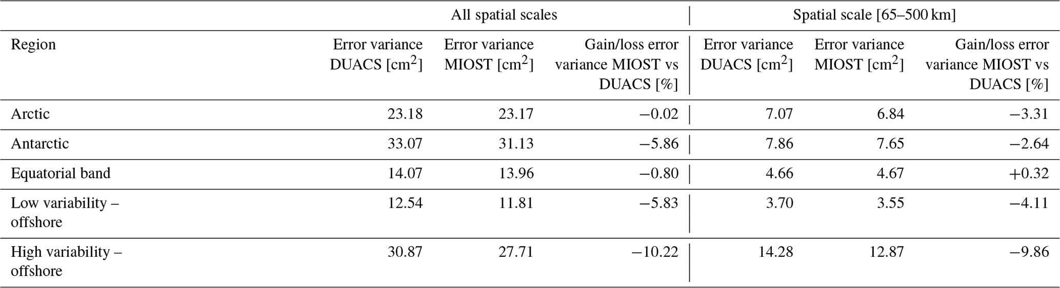
We present a new gridded sea surface height and current dataset produced by combining observations from nadir altimeters and drifting buoys. This product is based on a multiscale and multivariate mapping approach that offers the possibility to improve the physical content of gridded products by combining the data from various platforms and resolving a broader spectrum of ocean surface dynamic than in the current operational mapping system. The dataset covers the entire global ocean and spans from 1 July 2016 to 30 June 2020. The multiscale approach decomposes the observed signal into different physical contributions. In the present study, we simultaneously estimate the mesoscale ocean circulations as well as part of the equatorial wave dynamics (e.g. tropical instability and Poincaré waves). The multivariate approach is able to exploit the geostrophic signature resulting from the synergy of altimetry and drifter observations. Sea-level observations in Arctic leads are also used in the merging to improve the surface circulation in this poorly mapped region. A quality assessment of this new product is proposed with regard to an operational product distributed in the Copernicus Marine Service. We show that the multiscale and multivariate mapping approach offers promising perspectives for reconstructing the ocean surface circulation: observations of leads contribute to improvement of the coverage in delivering gap-free maps in the Arctic and observations of drifters help to refine the mapping in regions of intense dynamics where the temporal sampling must be accurate enough to properly map the rapid mesoscale dynamics. Overall, the geostrophic circulation is better mapped in the new product, with mapping errors significantly reduced in regions of high variability and in the equatorial band. The resolved scales of this new product are therefore between 5 % and 10 % finer than the Copernicus product (https://doi.org/10.48670/moi-00148, Pujol et al., 2022b).

1 Introduction

Several oceanographic applications (e.g. operational oceanography, marine weather, and climate monitoring) rely on high-quality observational datasets. The European Union (EU) Copernicus Marine and Climate Change Services provide operational services and indicators on the observed state of the climate. Sea-level and surface currents are, among others, key variables distributed by the services. They are also listed as Essential Climate Variables (ECVs) for the detection of climate change and the characterization of climate system variability (Bojinski et al., 2014).

As part of the Copernicus Services, the Sea Level Thematic Assembly Centre (SL-TAC) delivers near-real-time and delayed-time sea-level and surface current products (along-track Level-3 and gridded Level-4 products) that are used by the ocean science community to study, understand, and monitor the evolution of the ocean system. These products do not resolve the entire spectrum of the ocean surface variability; they have resolution limits of about 60 km for the along-track products (Dufau et al., 2016) and >200 km × 20 d for the gridded products (Ballarotta et al., 2019), but recent nadir altimetry instruments, such as the new Sentinel-3A and 3B SAR missions, or future missions based on large swath technologies (e.g. the upcoming Surface Water and Ocean Topography (SWOT) mission) offer, for example, the possibility of observing finer ocean structures (Morrow et al., 2019), which could be used to provide better gridded product resolution.

In addition, the growing needs to develop observing systems or methods with finer spatial scales and higher frequencies have been identified by the ocean scientific community and the Copernicus Services as research and development priorities to serve Copernicus marine users and decision-makers (see, for example, International Altimetry Team, 2021, or the “Copernicus Marine Service Evolution Strategy: R&D priorities – Version 5 June 30, 2021” document, https://marine.copernicus.eu/sites/default/files/media/pdf/2021-09/CMEMS Service_evolution_strategy_RD_priorities_v5-June-2021.pdf, last access: 1 December 2022). Therefore, with the support of the French Space Agency (CNES), the development of new experimental products has been undertaken, aiming at improving the resolution of the current Level-3 and Level-4 sea-level products (Mulet et al., 2021a; Ballarotta et al., 2020; Ubelmann et al., 2022; Prandi et al., 2021) and preparing operational systems for the SWOT era (Ubelmann et al., 2015, 2021; Le Guillou et al., 2021; Beauchamp et al., 2020).

The present study focuses on the development and assessment of experimental global gridded products based on a recent multiscale and multivariate mapping approach (Ubelmann et al., 2021, 2022) and applied to real Earth observations. Here we investigate the possibility of improving the content of gridded products in combining the data from various platforms (in situ and satellite) and in resolving a larger spectrum of the ocean surface dynamic than in current operational products.

The paper is structured as follows: the data sources and merging methods used in this study are described in Sect. 2. Section 3 presents the experiments and validation metrics. The quality assessment of the new products is proposed in Sect. 4. The key results are then summarized in Sect. 5.

2 Data and methods

2.1 Data sources

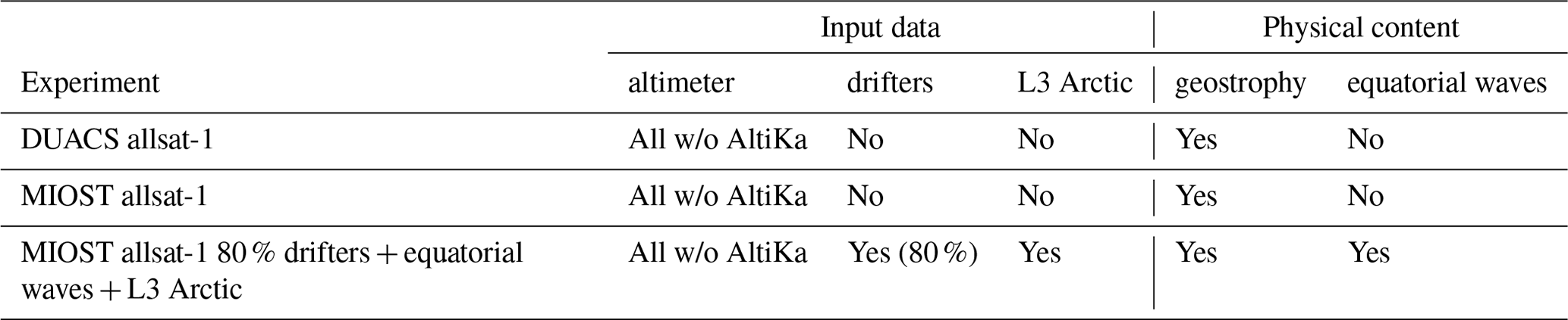
The mapping method used in this study takes input data from remote sensing and in situ observations, which are summarized in Table 1 and described below.

Table 1 List of observation datasets used in this study.

2.1.1 Sea-level anomaly products

The global ocean sea surface height (SSH) observations are from the (delayed time, DT) Level-3 altimeter satellite along-track data, reprocessed in 2021 and distributed by the EU Copernicus Marine Service (product reference SEALEVEL_GLO_PHY_L3_MY_008_062, https://doi.org/10.48670/moi-00146, Pujol et al., 2022a). These data cover the period from 1 January 1993 to 31 December 2020 over the world ocean (excluding ice-covered areas; see, for example, Fig. 1) and are available at a sampling rate of 1 Hz (∼ 7 km spatial spacing). Homogenization and cross-validation are applied to the dataset to remove any residual orbit error, long-wavelength error (lwe), large-scale biases, and discrepancies between different data streams. The list of geophysical and environmental corrections applied to the datasets is described in the quality information document (Taburet et al., 2021) and summarized below in Eq. (1). In this study, unfiltered sea-level anomalies (SLAs) corrected with dynamic atmospheric correction (dac), ocean tide, and lwe corrections are considered in the multiscale and multivariate mapping.

$$\begin{array}{}\text{(1)}& \begin{array}{rl}\mathrm{SLA}& =\mathrm{orbit}-\mathrm{range}-\sum \left(\text{environmental corrections}\right)\\ & -\sum \left(\text{geophysical corrections}\right)-\text{mean sea surface,}\end{array}\end{array}$$

where $\sum \text{(environmental corrections)}=\text{wet tropospheric}+\text{dry tropospheric}+\mathrm{ionospheric}+\text{sea-state bias}$, $\sum \text{(geophysical corrections)}=\text{solid earth tide}+\text{load tide}+\text{ocean tide}+\text{pole tide}+\text{dynamic atmospheric correction}$ (see Taburet et al., 2021, for the references associated with each mission correction). The mean sea surface used here is the CNES-CLS18 (Mulet et al., 2021b).

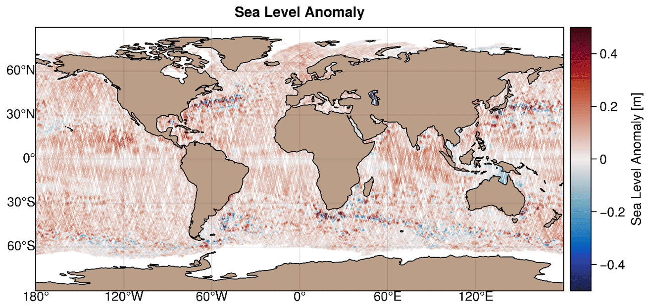
Figure 1 Example of sea-level altimetry coverage for a 7 d period (from 1 July 2019 to 7 July 2019). Colour scale represents the sea-level anomaly amplitude in metres. For this time interval, data originate from six altimeters: Jason-3, Sentinel-3A, Sentinel-3B, SARAL/AltiKa, Cryosat-2, and Haiyang-2A.

2.1.2 Sea-level anomaly products in Arctic leads

In the polar regions, satellite sea-level observations are limited by the sea ice. Thanks to dedicated processing, sea level can however be estimated within fractures in the ice (leads). The echoes from the altimeters over the ice-covered region are classified to identify peaky waveforms corresponding to lead echoes. Range estimation is then made with specific retracking methods, and it is corrected from instrumental and geophysical corrections to obtain a sea-level anomaly (Prandi et al., 2021). To ensure continuity with the open ocean, the corrections are derived from the global ocean Level-3 along-track processing (Taburet et al., 2021) when possible. The noticeable exceptions concern (1) the wet tropospheric correction that comes from the European Centre for Medium-Range Weather Forecasts (ECMWF) model since onboard radiometer estimates are not reliable over ice, (2) the sea-state bias correction which is not applied since waves and winds are considered small over leads, and (3) orbit error corrections which are not applied as they are difficult to compute over this small region. Then a constant bias of ∼ 8 cm is applied for each mission to ensure continuity with the SEALEVEL_GLO_PHY_L3_MY_008_062 open-ocean SLA previously described. These products cover the Arctic region (up to 88^∘ N) at a sampling rate of 20 Hz (∼ 350 m) for three altimetry missions: SARAL/AltiKa, Sentinel-3A, and CryoSat-2 (Fig. 2 and Table 2).

Table 2 Arctic leads' product characteristics. LRM: low-resolution mode. TFMRA: threshold first-maximum retracker algorithm.

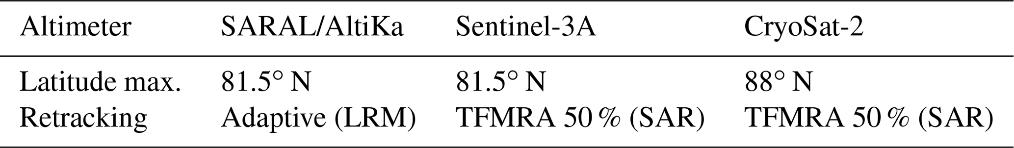
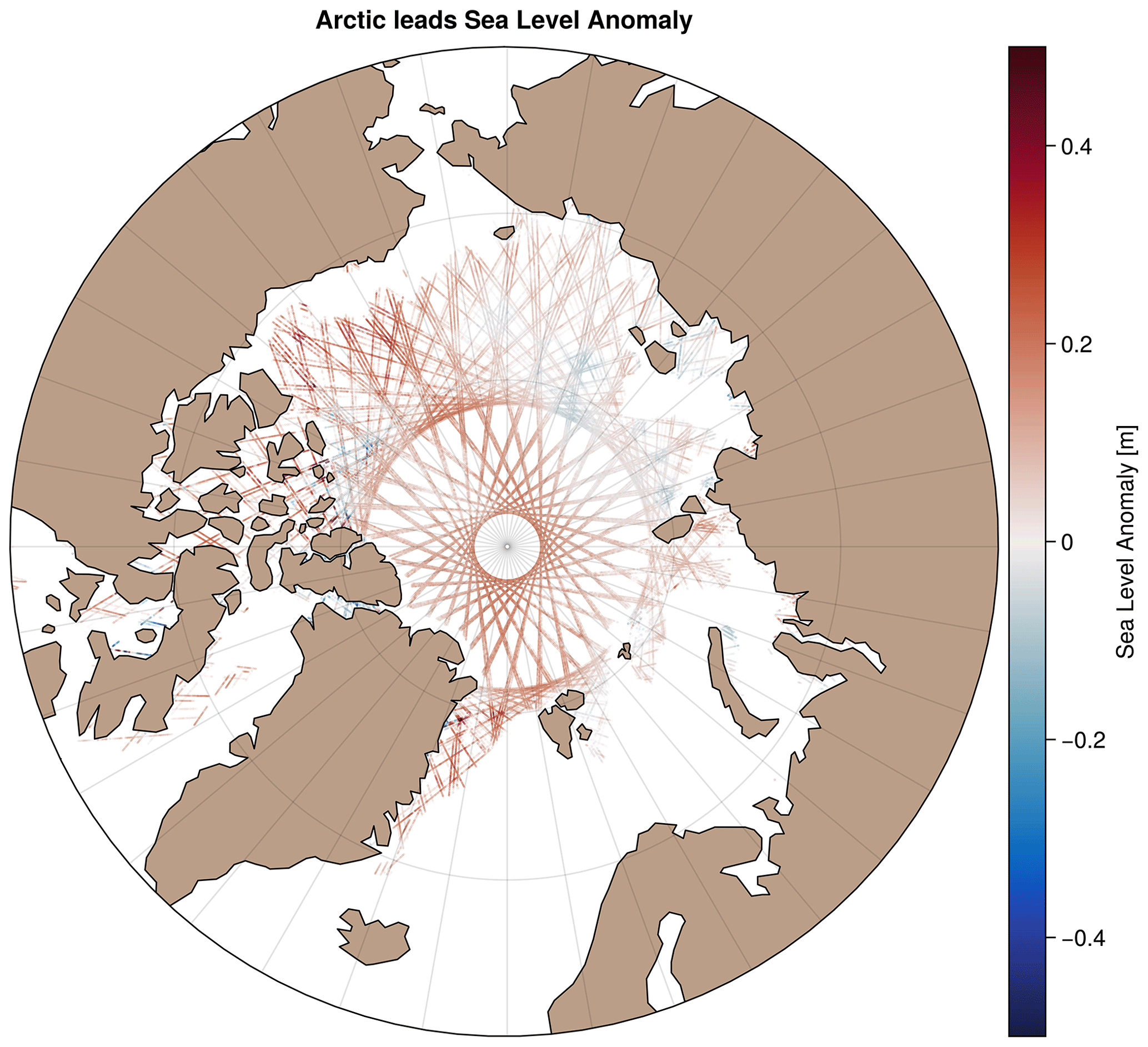
Figure 2 Example of Arctic leads' sea-level altimetry coverage for a 7 d period (from 1 July 2019 to 7 July 2019). Colour scale represents the sea-level anomaly amplitude in metres.

2.1.3 Geostrophic current anomaly products

To further constrain the surface circulation, we used delayed-time horizontal surface velocities from the NOAA's Atlantic Oceanographic and Meteorological Laboratory (AOML) Surface Velocity Program (SVP; Lumpkin and Centurioni, 2019). The data cover the entire world ocean and are available at a 6 h frequency. The SVP drifters are designed to follow the 15 m depth circulation, which is the centre depth of their drogues. When the drogue is lost, they follow the surface current but are also under the direct influence of the wind. AOML distributes a flag to indicate whether the drogue is lost or not (Lumpkin et al., 2013). These data are also distributed by the IN SITU Thematic Assembly Centre of the EU Copernicus Marine Service (see Product User Manual; http://marine.copernicus.eu/documents/PUM/CMEMS-INS-PUM-013-044.pdf, last access: 9 January 2023) with an additional wind slippage correction for undrogued buoys derived from the Rio (2012) methodology. For the study, the undrogued and drogued drifters are selected over the global ocean and the period from 1 June 2016 to 31 July 2020. Note that for specific experiments described hereafter, we excluded drifters' trajectories between −10^∘ S and 10^∘ N (e.g. Fig. 3) to isolate and evaluate only the impact of the equatorial wave's mode in this region. As in Mulet et al. (2021a), we computed the geostrophic velocity anomaly components, which are defined as

$$\begin{array}{}\text{(2)}& {\displaystyle }\begin{array}{rl}{U}_{\mathrm{anom}}& =U_{\mathrm{buoy}}-U_{\mathrm{ekman}}-U_{\mathrm{stokes}}-U_{\mathrm{inertial}}-U_{\mathrm{tidal}}\\ & -U_{\mathrm{ahf}}-U_{\mathrm{slip}}-U_{\mathrm{mdt}}\end{array}\text{(3)}& {\displaystyle }\begin{array}{rl}{V}_{\mathrm{anom}}& =V_{\mathrm{buoy}}-V_{\mathrm{ekman}}-V_{\mathrm{stokes}}-V_{\mathrm{inertial}}-V_{\mathrm{tidal}}\\ & -V_{\mathrm{ahf}}-V_{\mathrm{slip}}-V_{\mathrm{mdt}},\end{array}\end{array}$$

where U_buoy (V_buoy) is the drifter's zonal (meridional) velocity. Each component is corrected as follows.

• The wind-driven component U_ekman (V_ekman) uses an update of the model used in Mulet et al. (2021a) and described in Etienne (2021a). The Ekman component is not available in the Mediterranean basin, so there is no drifter used in this region for the study. In this recent version, ERA5 wind stress (Hersbach et al., 2018) replaces the ERA Interim data, and the equatorial symmetry of the wind driven parameters is removed.

• The Stokes drift U_stokes (V_stokes) from ERA5 reanalysis (Hersbach et al., 2018) is also removed from the surface drifter velocity (undrogued drifters). No Stokes drift is removed from the 15 m depth velocity, as this component is supposed to mostly vanish in the first 2–4 m.

• The wind slippage is the direct effect of the wind on the buoy U_slip (V_slip). This correction is significant only in the case of drogue loss (Etienne et al., 2021), when the drifters are advected by the surface current.

Then the data are filtered from the tidal and inertial velocities U_inertial+U_tidal (V_inertial+V_tidal) as well as the residual high-frequency ageostrophic signal U_ahf (V_ahf). Finally, the mean geostrophic velocity (CNES-CLS2018; Mulet et al., 2021b) U_mdt (V_mdt) is subtracted to obtain the geostrophic velocity anomaly.

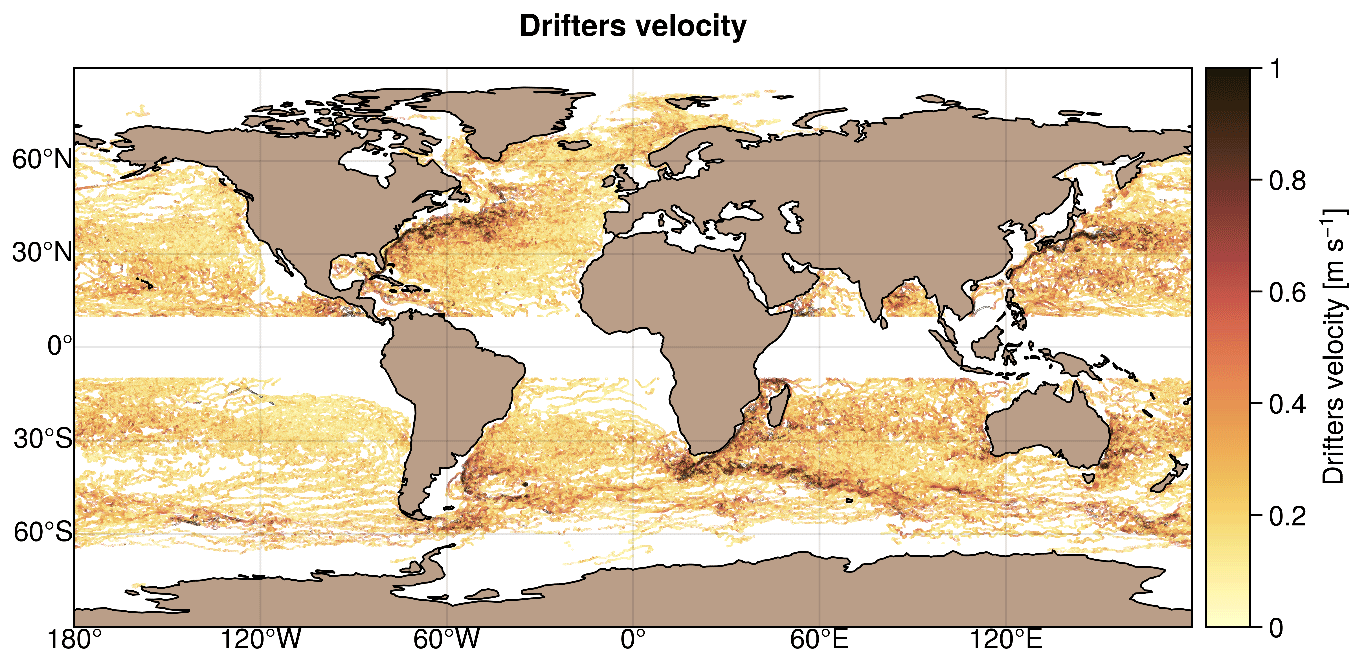
Figure 3 Example of the drifter's trajectory coverage for the period 1 January 2019 to 31 December 2019. Colour scale represents the velocity amplitude in metres per second (m s⁻¹).

2.2 Methods

Two mapping methods are compared in this study: the operational DUACS (Data Unification and Altimeter Combination System) mapping approach and the multiscale and multivariate MIOST (Multiscale Inversion of Ocean Surface Topography) mapping approach. Each method is described in detail in reference articles, such as Le Traon et al. (1998, 2003), Ducet et al. (2000), or Pujol et al. (2016) for the DUACS method and Ubelmann et al. (2021, 2022) for the MIOST method. A description of the methods is given in Appendix A, and we propose hereafter to focus on the specific developments and processes that are considered in this study.

It is important to mention that DUACS maps are constrained by a single-scale covariance function (Arhan and Colin de Verdière, 1985; Le Traon et al., 1998) and focus mainly on the geostrophic circulation (i.e. processes with typical space and timescales >100 km, 10 d). Consequently, they do not resolve the full spectrum of ocean surface variability. It is, for example, the case for the equatorial surface dynamics (see, for example, Fig. 7). While slow Rossby waves are already resolved within geostrophy in DUACS maps, faster equatorial waves such as Poincaré waves are filtered out, even though the space–time coverage of altimetry data allows for sampling of large-scale waves with periods of 4–10 d and more (Farrar and Durland, 2022). The multiscale approach proposed by the MIOST method offers the possibility to solve some of the missing surface variabilities in DUACS, accounting for the covariances of various surface processes in a single inversion. The covariance functions in the MIOST system are expressed as wavelet modes, and the inversion is performed in this space using a variational approach (Ubelmann et al., 2021). In the following, we focus on the main components that have been tested in this study with the MIOST method: the geostrophy component already investigated in Ubelmann et al. (2021) and two new components associated with the equatorial wave's dynamic.

The geostrophy component follows the same formulation provided in Ubelmann et al. (2021) (see their Sect. 2.3.2.1, where the analytical formula of the ensemble of wavelet elements is given) and is also reported in Appendix A. The covariance function associated with the geostrophy component is plotted for a given point (5^∘ N, 210^∘ E) in Fig. 4a and c, shown as a function of space (bottom left panel) and as a function of time (top left panel). This covariance function is similar to what is currently used for altimetry mapping with DUACS.

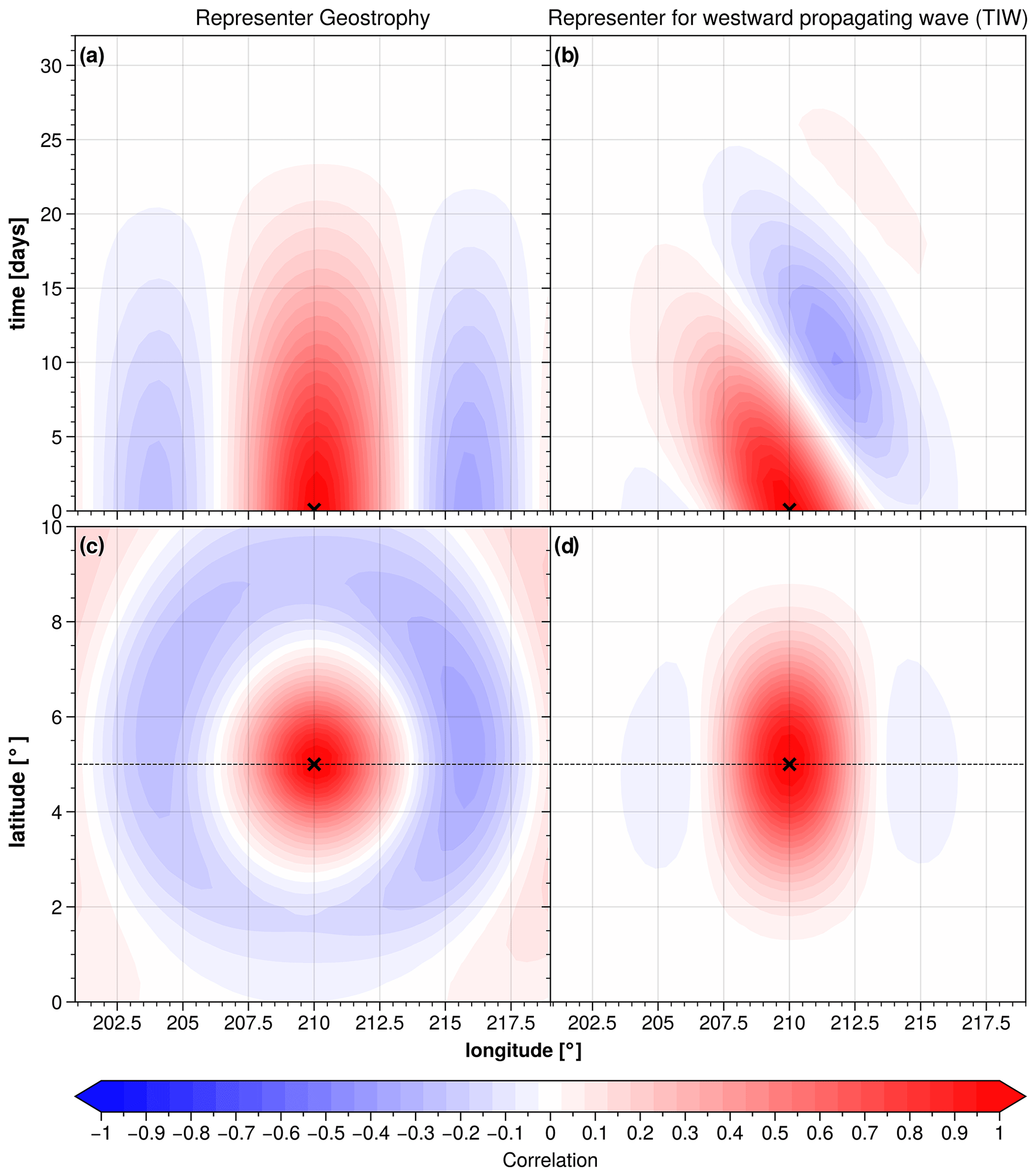
Figure 4 Example of spatio-temporal covariance models at (5^∘ N, 210^∘ E) for (a, c) the geostrophy component and for (b, d) a westward-propagating wave component, e.g. TIW.

In the present study, we simultaneously estimate the surface signatures of the geostrophy and equatorial tropical instability waves (TIWs) and Poincaré waves. As for the geostrophy component, the equatorial wave covariances are expressed as a reduced wavelet basis, with typical wavelength and propagation speed given in the literature (e.g. Shinoda et al., 2009; Farrar, 2008, 2011; Farrar and Durland, 2012; Tanaka and Hibiya, 2019). For Poincaré waves, we built an ensemble of wavelets between 10^∘ S and 10^∘ N which follow the dispersion relation (Matsuno, 1966):

$$\begin{array}{}\text{(4)}& \mathit{\omega }=\sqrt{k^{\mathrm{2}}\cdot c^{\mathrm{2}}+\mathit{\beta }\cdot c\cdot \left(\mathrm{2}\cdot n+\mathrm{1}\right)},\end{array}$$

where ω is the time frequency, $c=\pm \mathrm{2.8}$ m s⁻¹ is the Poincaré wave propagation speed (considered a constant here), k is the spatial wavenumber, and n is a positive integer defining the wave mode. The wavelets are localized with a Hamming window with half-widths of 1000 km in the zonal direction, 300 km in the meridional direction, and 5 d in the temporal direction. For the TIW component, we also built an ensemble of wavelets between 10^∘ S and 10^∘ N which follow the dispersion relation (Matsuno, 1966):

$$\begin{array}{}\text{(5)}& \mathit{\omega }=c\cdot k,\end{array}$$

where ω is the time frequency, $c=-\mathrm{0.5}$ m s⁻¹ is the TIW propagation speed (considered a constant here), and k is the spatial wavenumber. The wavelets are localized here with a Hamming window with half-widths of 500 km in the zonal direction, 300 km in the meridional direction, and 20 d in the temporal direction. The covariance function for a westward-propagation-wave-like TIW is illustrated in Fig. 4b and d for a given point (5^∘ N, 210^∘ E), shown as a function of space (bottom right panel) and as a function of time (top right panel). Note that for Poincaré waves, both eastward and westward propagation is considered. A more detailed description of the equatorial wave's components implemented in MIOST is provided in Appendix A.

3 Experiments and validation metrics

3.1 Experiments

We produced 4 years (from 1 July 2016 to 30 June 2020) of SSH maps using the MIOST multiscale and multivariate approach by combining the Level-3 altimeter dataset from SARAL/AltiKa, Envisat, Jason-1, Jason-2, Jason-3, Cryosat-2, Haiyang-2A, Haiyang-2B, Sentinel-3A, and Sentinel-3B missions, the Level-3 Arctic lead sea-level anomaly products from SARAL/AltiKa, Sentinel-3A, and CryoSat-2 missions, and geostrophic current anomaly data from the AOML drifter database. These MIOST products are available on the AVISO + (Archivage, Validation et Interprétation des données des Satellites Océanographiques) website (see Sect. 5, “Data availability”, for more details).

Specific maps were also made to quantitatively assess the quality of these MIOST products. Table 3 summarizes the list of experiments conducted in this study, indicating the input data used in the mapping and the physical content of the maps.

DUACS allsat-1 and MIOST allsat-1 experiments focus on the geostrophic variability. These SSH maps were produced from six altimeters (Jason-3, Cryosat-2, Sentinel-3A, Sentinel-3B, Haiyang-2A, Haiyang-2B) for the period 1 January 2019 to 31 December 2019, excluding one altimeter (Saral/AltiKa, over open-ocean region) from the mapping to perform independent assessments. The MIOST allsat-1 80 % drifters + equatorial waves + L3 Arctic experiment focuses on the geostrophic and equatorial wave variabilities. This experiment is based on (1) 80 % of the drifter data, (2) the six altimeters previously mentioned over ocean, and (3) lead altimeter observations. The Saral/AltiKa dataset (over open-ocean region) and the remaining 20 % of the drifter trajectories were here excluded from the mapping to perform independent assessments. Note that for these specific maps, drifter trajectories between −10^∘ S and 10^∘ N (e.g. Fig. 3) were also excluded to evaluate only the impact of the equatorial wave's mode in this region.

Table 3 List of mapping experiments with the input data and physical content considered.

3.2 Validation metrics

The validation metrics are based on statistical and spectral analysis.

One quantitative assessment is based on the comparison between SSH maps and independent SSH along-track data. This diagnostic follows three main steps: (1) the SSH gridded data are interpolated to the locations of the independent SSH along-track, geo-referenced by their longitude, latitude, and time; (2) the difference SSH${}_{\mathrm{error}}={\mathrm{SSH}}_{\text{map}}-{\mathrm{SSH}}_{\text{along-track}}$ is calculated; and (3) a statistical analysis on the SSH_error is performed in 1^∘ × 1^∘ longitude × latitude boxes. Prior to the statistical analysis, a filtering operation can be applied to isolate the spatial scales of interest. For example, the analysis can be performed over the spatial range [65–500 km] typically representative of the medium mesoscale ocean signal. This excludes the noisy part of the reference signal (along-track) as well as possible large-scale biases (scale >500 km). In the study, the validation metric is based on the error variance scores in 1^∘ × 1^∘ longitude × latitude boxes (or averaged over a specific region of interest), defined as

$$\begin{array}{}\text{(6)}& {\mathit{\sigma }}_{\mathrm{err}}\left(x,y\right)={\displaystyle \frac{{\sum }_{t=\mathrm{1}}^N{\left({\mathrm{SSH}}_{\mathrm{error}}\left(x,y,t\right)-\stackrel{\mathrm{‾}}{{\mathrm{SSH}}_{\mathrm{error}}\left(x,y,t\right)}\right)}^{\mathrm{2}}}{N}}.\end{array}$$

The similar statistical analysis can also be performed on the geostrophic velocity errors $U_{\mathrm{error}}=U_{\text{map}}-U_{\mathrm{drifter}}$ for the zonal component and $V_{\mathrm{error}}=V_{\text{map}}-V_{\mathrm{drifter}}$ for the meridional component.

The comparison of the error variance score between two experiments informs about the gain or reduction Δ of the mapping error; for example,

$$\begin{array}{}\text{(7)}& \mathrm{\Delta }=\mathrm{100}\cdot {\displaystyle \frac{{\mathit{\sigma }}_{\mathrm{err}}\left(\mathrm{EXP}\mathrm{2}\right)-{\mathit{\sigma }}_{\mathrm{err}}\left(\mathrm{EXP}\mathrm{1}\right)}{{\mathit{\sigma }}_{\mathrm{err}}\left(\mathrm{EXP}\mathrm{1}\right)}}\end{array}$$

The previous diagnosis is undertaken in physical space (space–time space). For a more descriptive assessment by wavelength and to avoid spatio-temporal filtering of independent and study datasets, diagnostics can be performed in frequency space, using spectral analysis of SSH altimetry and gridded datasets. More specifically, a spectral analysis can be applied to altimetry data to estimate the effective resolution of gridded SSH products. It is described, for example, in Ballarotta et al. (2019). Here, we recall the main processing steps for the estimation of the effective resolution: (1) the SSH_map data are interpolated to the locations of independent SSH_along-track data, (2) the along-track and interpolated data are divided into overlapping segments of 1500 km length every 300 km, (3) each segment is stored in a database and referenced by its median coordinates (longitude, latitude), and (4) finally, between latitudes 90^∘ N–90^∘ S and longitudes 0^∘–360^∘ E, we consider 10^∘ × 10^∘ longitude × latitude boxes for the global products every 1^∘ increment. All available segments referenced in the 10^∘ × 10^∘ box are selected to compute the mean power spectral densities of the independent signal (SSH_along-track) and the mapping error (SSH_map−SSH_along-track). Before the spectral calculation, the signals are detrended, and a Hanning window is applied. The signal-to-noise (SNR) ratio (Eq. 8) is then derived from the power spectral density (PSD) of the along-track SSH (SSH_along-track) and the PSD of the error (SSH_map−SSH_along-track). As in Ballarotta et al. (2019), the effective resolution is then given by the wavelength λs where the SNR(λs) is 2 (Eq. 9), i.e. the wavelength where the SSH_error is 2 times lower than the signal SSH_along-track.

$$\begin{array}{}\text{(8)}& {\displaystyle }\mathrm{SNR}\left(\mathit{\lambda }\right)={\displaystyle \frac{\mathrm{PSD}\left({\mathrm{SSH}}_{\text{along-track}}\right)\left(\mathit{\lambda }\right))}{\mathrm{PSD}\left({\mathrm{SSH}}_{\mathrm{error}}\right)\left(\mathit{\lambda }\right)}}\text{(9)}& {\displaystyle }\mathrm{SNR}\left(\mathit{\lambda }s\right)=\mathrm{2}\end{array}$$

4 Results

4.1 Qualitative assessment

Here we qualitatively assess the gridded products from the DUACS allsat-1 and MIOST allsat-1 80 % drifters + equatorial waves + L3 Arctic experiments. The SLA maps from the DUACS and MIOST mapping approaches are relatively similar in the subpolar region, as illustrated in Fig. 5 by an example of SLA reconstruction on 15 February 2019 for (a) the DUACS mapping approach and (b) the MIOST mapping approach. More significant differences take place in the Arctic basin: in contrast to the DUACS products, the use of Arctic lead observations in MIOST offers the possibility to extend sea-level mapping into ice-covered area and thus to deliver gap-free maps to end users (Fig. 5b).

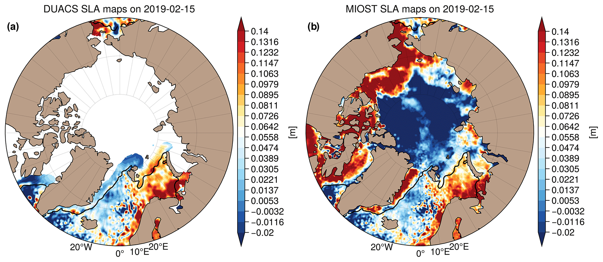
Figure 5 Example of sea-level anomaly maps on 15 February 2019 over the Arctic region constructed with the DUACS mapping approach (a) and with the MIOST mapping approach (b). The black line contour indicates the 15 % sea-ice concentration from the OSI-SAF product.

From a global perspective, the MIOST maps are slightly more energetic than the DUACS maps as illustrated in Fig. 6 with the variance maps and their differences. The difference between MIOST and DUACS variance maps (Fig. 6c) indicates regions of higher variability in the MIOST maps (>10 %) than in the DUACS maps, such as in the equatorial band, regions of low variability at mid-latitudes, and coastal and polar regions. Tropical ocean regions are prone to lower SSH variability (10 %) in the MIOST maps than in the DUACS maps.

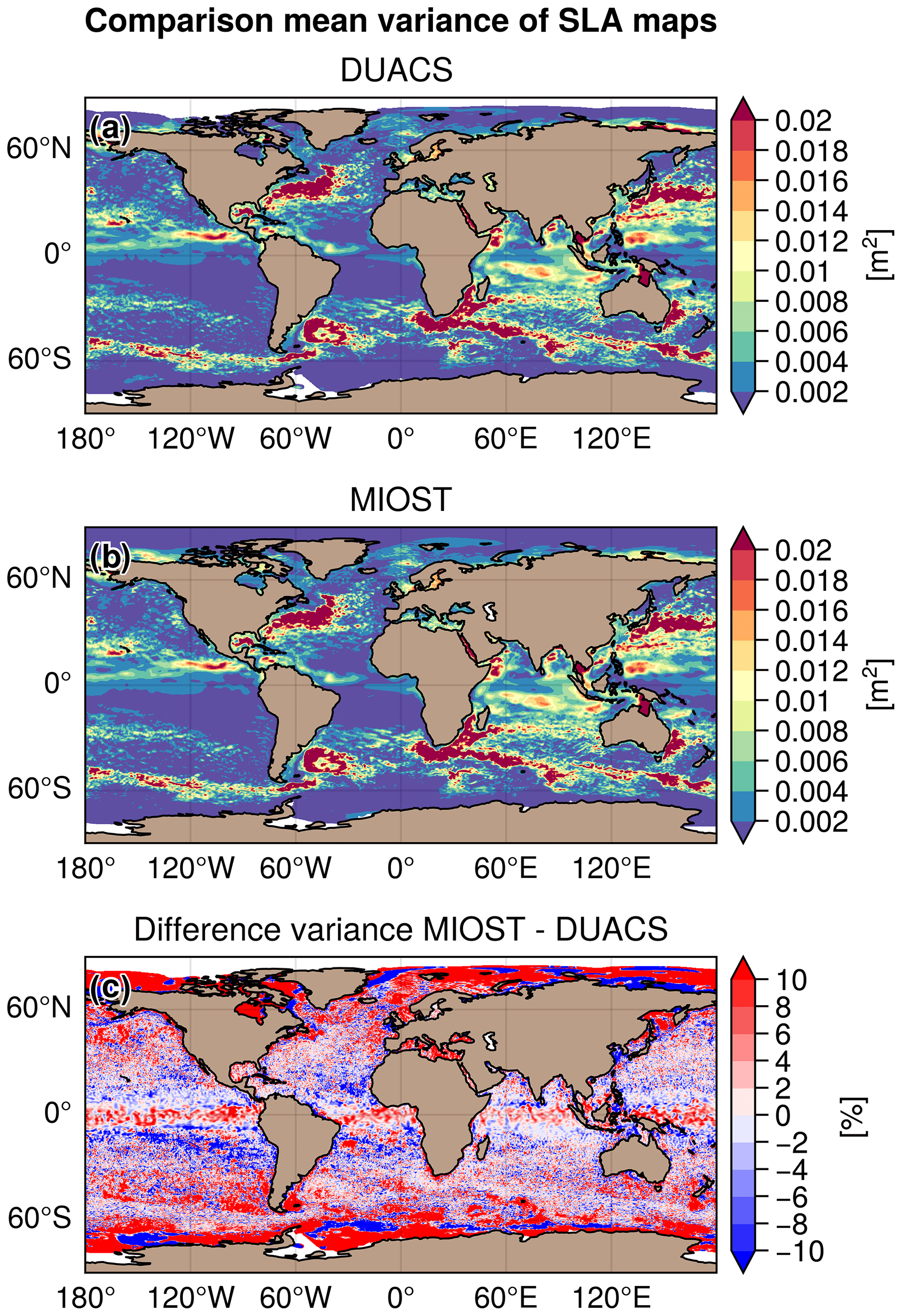
Figure 6 Variance (in m²) of sea-level anomaly maps constructed with (a) the DUACS approach, (b) the MIOST approach, and (c) the difference between the MIOST and DUACS variance maps expressed in percent.

The large SSH variability in the equatorial band of the MIOST maps is mainly associated with the equatorial wave components. The zonal wavenumber–frequency spectrum of SSH in the Pacific has been investigated in several studies (e.g. Shinoda et al., 2009; Farrar, 2008, 2011) to examine the SSH variability associated with tropical and equatorial waves. Figure 7 shows contours of the base 10 logarithm of power in the wavenumber–frequency space calculated from SSH in the equatorial Pacific (region [10^∘ S–10^∘ N], [180–280^∘ E]) for the period 2008 to 2018, for (a) DUACS, (b) MIOST with equatorial wave modes, and (c) the GLORYS12V1 reanalysis (Lellouche et al., 2018). The rapid equatorial wave dynamics are resolved in the GLORYS12v1 ocean numerical simulation (Fig. 7c): the zonal wavenumber–frequency spectrum of the SSH in the Pacific reveals significant spectral peaks at periods close to 4, 5, and 7 d for a wavelength >20^∘ in longitude. These peaks are associated with inertia-gravity (Poincaré) waves. These SSH variabilities for timescales smaller than 10 d are filtered in the DUACS mapping approach (Fig. 7a). In contrast, the MIOST multiscale mapping approach (MIOST allsat-1 80 % drifters + equatorial waves + L3 Arctic) resolves spectral peaks near 4, 5, and 7 d for wavelengths >20^∘ in longitude (Fig. 7b). We show in the next section that these equatorial wave modes in MIOST also contribute to a significant reduction of the mapping error in this region. For timescales >10 d, each dataset has relatively similar spectral contents, particularly the energetic westward propagation of equatorial Rossby waves for negative wavenumbers.

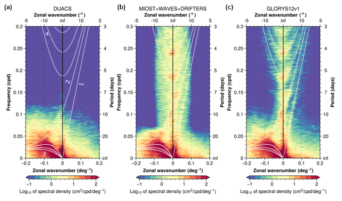
Figure 7 Zonal wavenumber–frequency spectrum of SLA in the equatorial Pacific computed for (a) DUACS, (b) MIOST with equatorial wave modes, and (c) the GLORYS12V1 reanalysis. White lines represent the theoretical dispersion relation curves for equatorial waves corresponding to the Kelvin [1], Yanai [2], Rossby [3], and Poincaré [4] waves.

4.2 Quantitative assessment

4.2.1 Mesoscale mapping assessments

The first assessment is a comparison of the DUACS allsat-1 and MIOST allsat-1 experiments. Both experiments aim to map the mesoscale circulation from altimetry data only. The SARAL/AltiKa altimeter and drifter sensors are not included in the mapping but are used as independent validation.

Sea-level anomaly quality

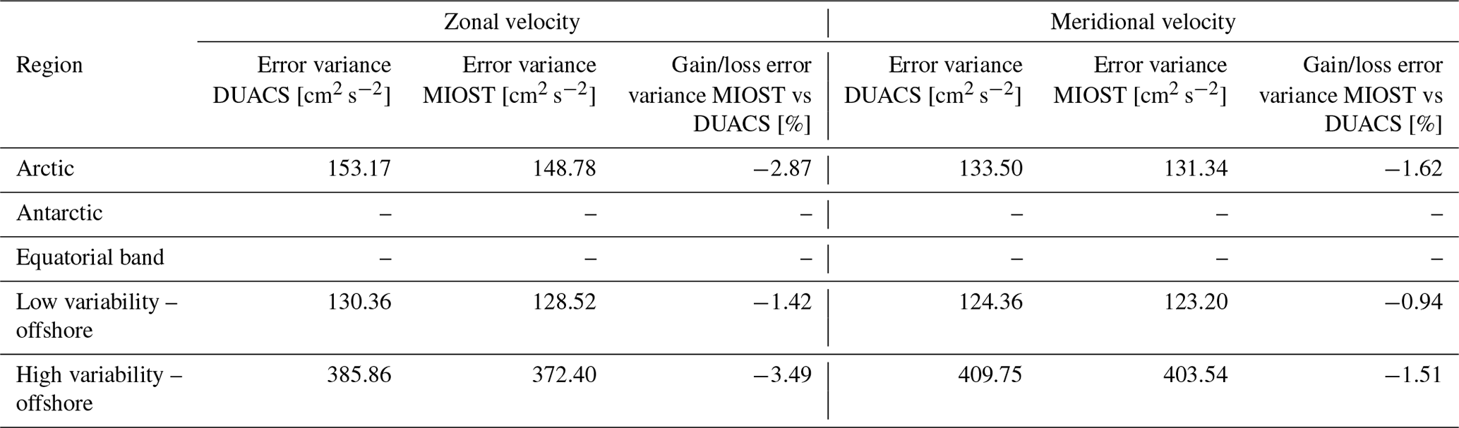
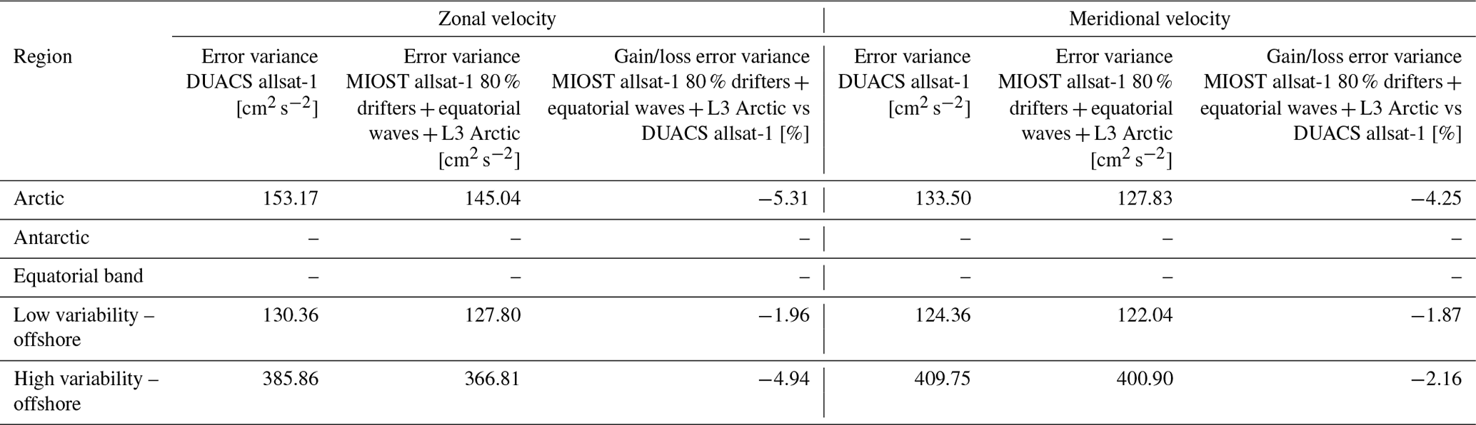
The largest SSH mapping error σ_err in DUACS allsat-1 reaches 50–100 cm² in the western boundary surface current and over the continental plateaus (Fig. 8a and b). In the offshore low-variability region, the error variance is <10 cm². Figure 8c and d show the difference in mapping error between the MIOST allsat-1 and DUACS allsat-1 experiments for all spatial scales and the spatial scale between 65 and 500 km, respectively. A blue (red) pattern means a reduction (increase) of the mapping error in MIOST compared to DUACS. For all spatial scales considered, MIOST mapping errors are smaller than those of DUACS, especially at mid-latitudes, with an average reduction in mapping error between 5 % and 10 %. The largest reduction in mapping error (∼ 10 %) is found in regions of high variability. In the intertropical region, MIOST and DUACS have similar scores. For spatial scales between 65 and 500 km, MIOST mapping errors are reduced by ∼ 10 % compared to DUACS in high-variability regions at mid-latitudes. In low-variability regions, the mapping error is between 3 and 4 % smaller with MIOST than with DUACS, but the mapping errors are locally larger with MIOST than with DUACS: for example, in the Argentine Sea, the Siberian plateau, and the New Zealand plateau. Table 4 summarizes the results of the comparison over different regions of interest (Arctic, Antarctic, equatorial band, low-variability region, and high-variability region). Overall, the geostrophic flows in the MIOST SSH maps are closer to the independent SARAL/AltiKa observations than those in DUACS maps.

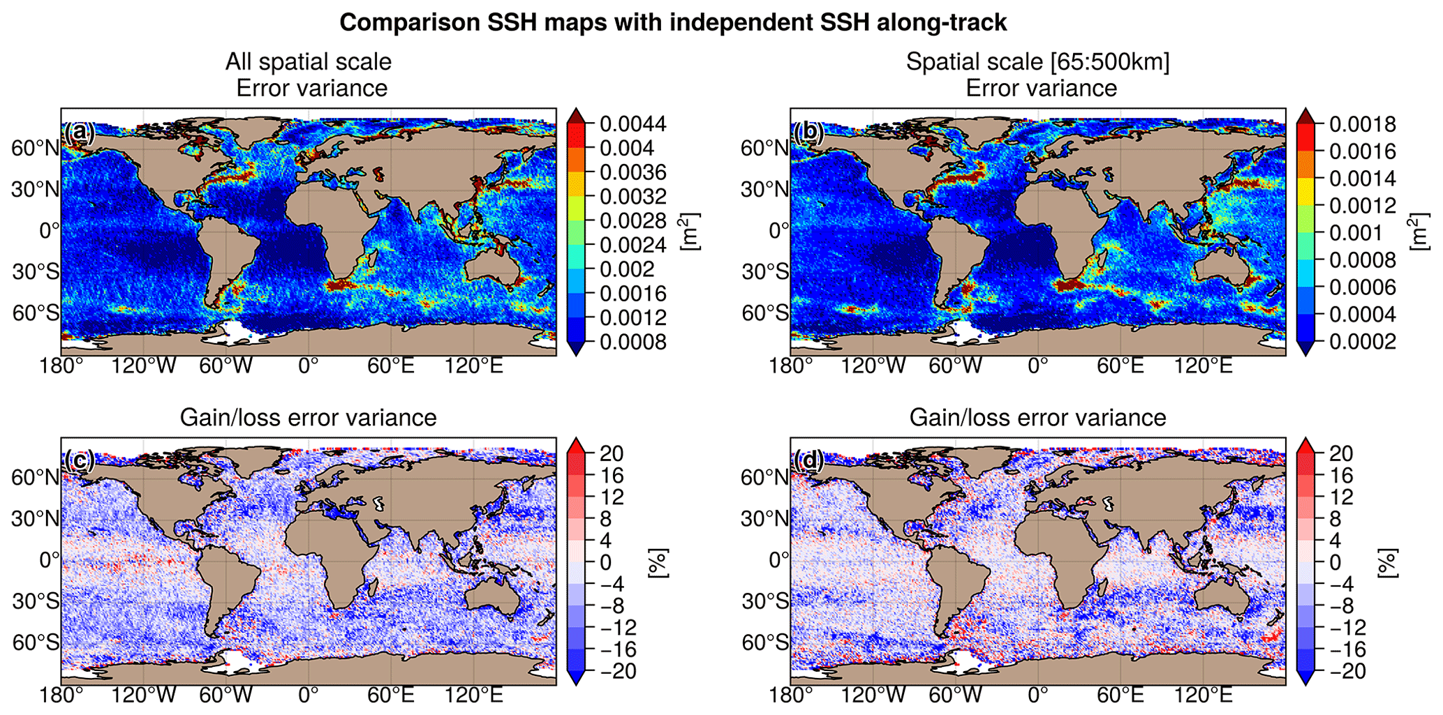
Figure 8 Variance of the difference SSH_map−SSH_along-track computed for the DUACS allsat-1 experiment and in considering (a) all spatial scales and (b) the spatial scale between 65 and 500 km. Gain/loss of the mapping error variance of SLA in the MIOST allsat-1 experiment relative to the DUACS allsat-1 mapping error variance for (c) all spatial scales and (d) the scale between 65 and 500 km. Blue colour means a reduction of error variance in MIOST.

Table 4 Regionally averaged mapping error variance and gain/reduction of error variance on the SSH variable between MIOST and DUACS.

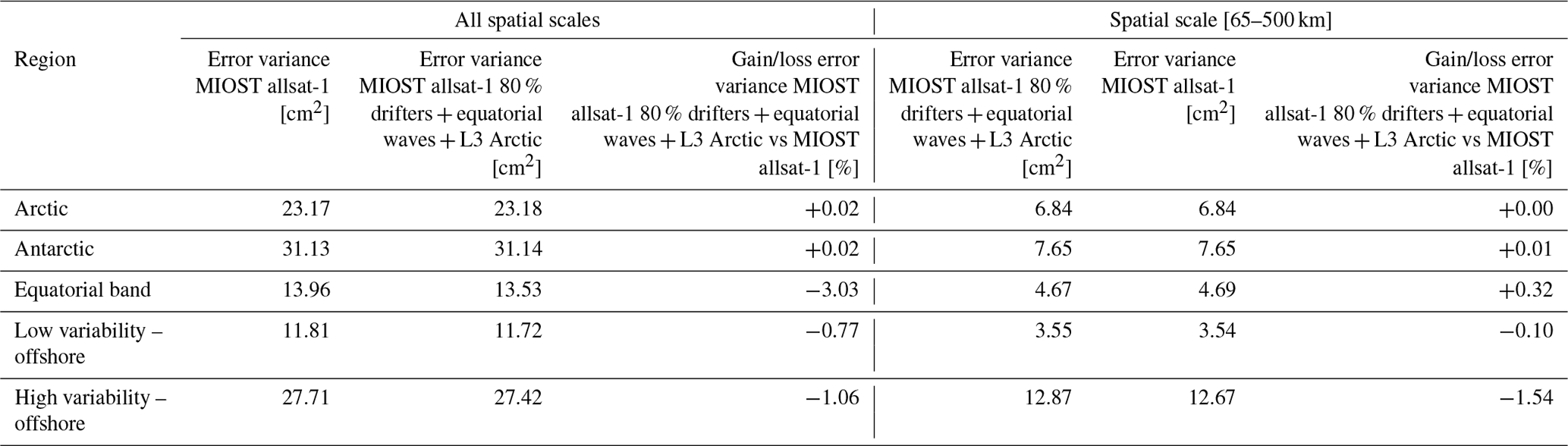
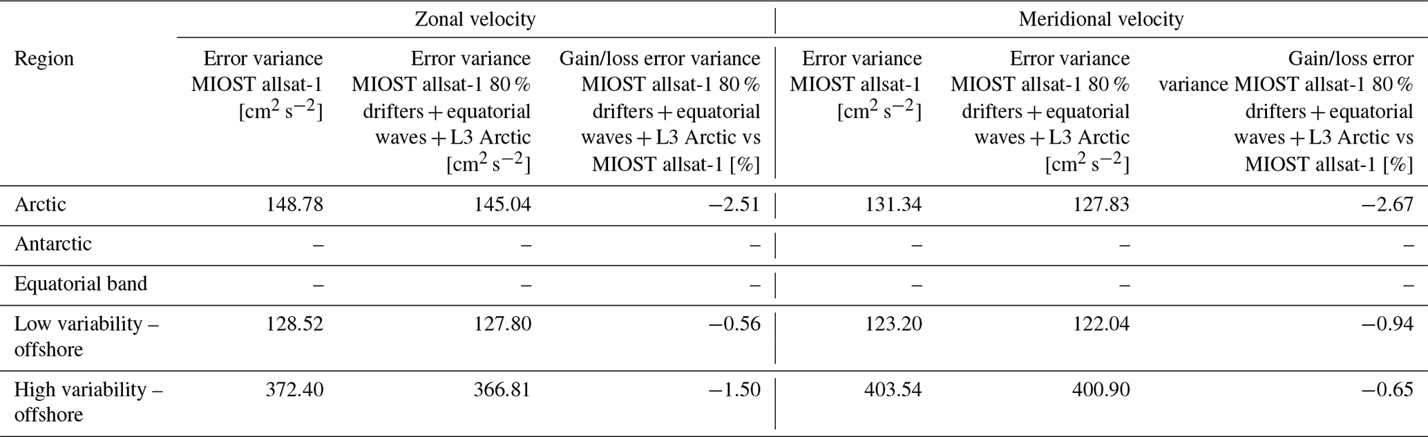
Geostrophic current quality

Figure 9a and b show the validation against the independent drifter velocity data in terms of mapping error σ_err for the zonal and meridional velocities. The largest mapping error σ_err in DUACS reaches 300 to 400 cm² s⁻² in the western boundary surface current (e.g. the Gulf Stream and the Kuroshio, Mozambique, and Agulhas currents). In offshore low-variability regions, the error variance is <80 cm² s⁻². The differences in mapping error between MIOST and DUACS are shown in Fig. 9c and d for zonal and meridional velocities, respectively. Mapping errors are smaller in MIOST than in DUACS, mainly in the core of the ocean gyres. In the intertropical region, the DUACS maps appear to be closer to the independent drifter velocities than MIOST. Table 5 summarizes the results of the comparison over different regions of interest (Arctic, Antarctic, equatorial band, low-variability region, and high-variability region). Overall, MIOST surface velocities are slightly closer to drifter velocities than the DUACS surface velocities.

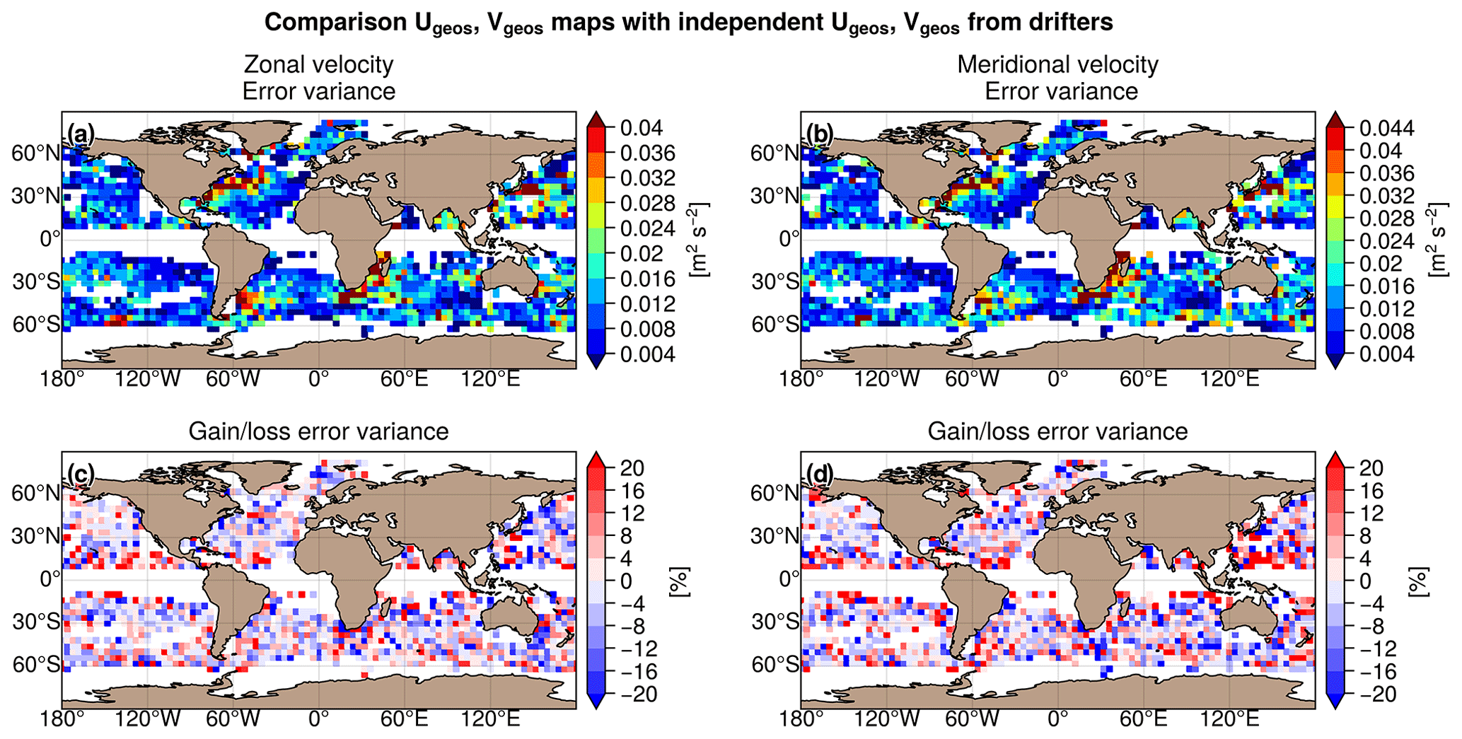
Figure 9 Variance of the difference U_map−U_drifter computed for the DUACS allsat-1 experiment and in considering (a) the zonal velocity component and (b) the meridional velocity component. Gain/loss of the mapping error variance of currents in the MIOST allsat-1 experiment relative to the DUACS allsat-1 mapping error variance for (c) the zonal velocity component and (d) the meridional velocity component. Blue colour means a reduction of error variance in MIOST.

Table 5 Regionally averaged mapping error variance and gain/reduction of error variance on the surface currents between MIOST and DUACS.

4.2.2 Contribution of equatorial wave modes and drifters' observations

The comparison of the MIOST allsat-1 80 % drifters + equatorial waves + L3 Arctic experiment with MIOST allsat-1 examines the impact of the equatorial waves' mode and the drifters' observations in the MIOST mapping approach.

Sea-level anomaly quality

The differences in mapping error between MIOST allsat-1 80 % drifters + equatorial waves + L3 Arctic and MIOST allsat-1 are shown in Fig. 10a and b for all spatial scales and the spatial scale between 65 and 500 km, respectively. For all spatial scales considered, we observe that the equatorial wave modes locally reduce the mapping error in the equatorial band by more than 10 %. However, coastal equatorial regions (e.g. Indonesian Archipelago, western and eastern parts of Africa, and South America) are prone to deterioration. This suggests that the equatorial wave mapping is not adapted in these coastal regions where different ocean processes are at play. In extra-equatorial regions, we evaluate the impact of drifter observations in MIOST. This impact is moderate on the SLA mapping (a few percent of difference in the mapping error variance), with a reduction of error variance mainly in the high-variability regions. For a spatial scale between 65 and 500 km (Fig. 10b), the equatorial wave modes deteriorate the mapping solution in the western and central equatorial Pacific Ocean and in the Indian Ocean, while a reduced mapping error is found in the eastern equatorial Pacific and the equatorial Atlantic. In the extra-equatorial region, the impact of drifter observations remains moderate (with 1.5 % error variance reduction in the high-variability region). Overall, the drifters reduce the mapping errors primarily in regions of intense dynamics where the temporal sampling must be sufficiently accurate to properly map the rapid mesoscale dynamics. Table 6 summarizes the results of the comparison over different regions of interest (Arctic, Antarctic, equatorial band, low-variability region, and high-variability region).

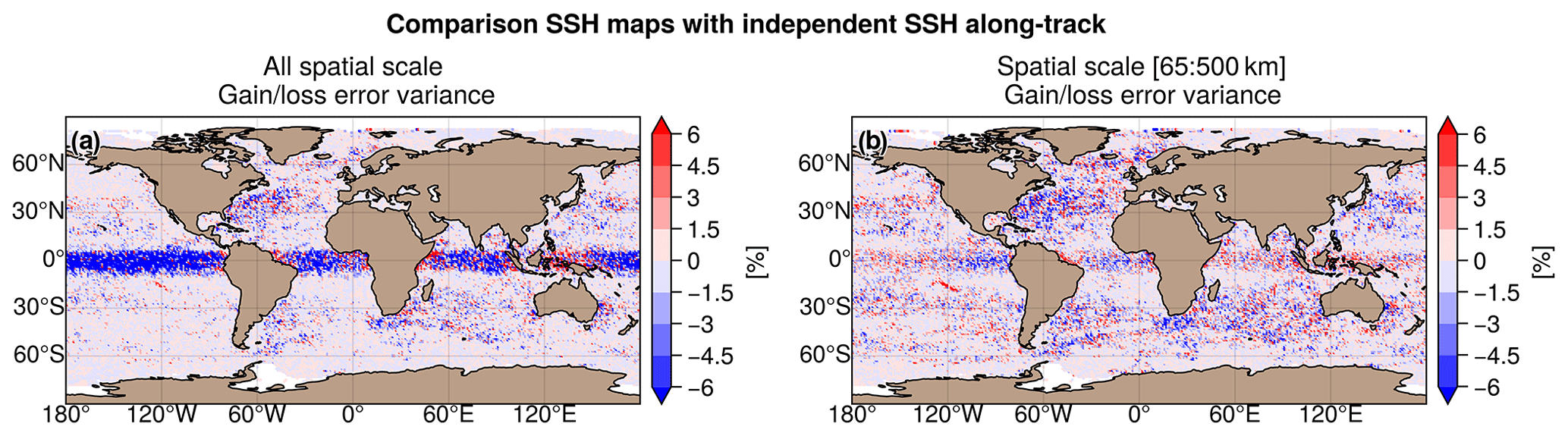
Figure 10 Gain/loss of the mapping error variance of SLA in the MIOST allsat-1 80 % drifters + equatorial waves + L3 Arctic experiment relative to the MIOST allsat-1 mapping error variance for (a) all spatial scales and (b) the scale between 65 and 500 km. Blue colour means a reduction of error variance in MIOST when drifters are included in the mapping and with equatorial wave parametrization.

Table 6 Regionally averaged mapping error variance and gain/reduction of error variance on the SSH variable between MIOST allsat-1 80 % drifters + equatorial waves + L3 Arctic and MIOST allsat-1.

Geostrophic current quality

The differences in mapping error of surface geostrophic currents between MIOST allsat-1 80 % drifters + equatorial waves + L3 Arctic and MIOST allsat-1 are shown in Fig. 11a and b for the zonal component and the meridional component of the velocity, respectively. It is difficult to draw conclusions from this diagnosis: the mapping errors are reduced with MIOST in some regions in the tropics (such as the Bay of Bengal) and in the Kuroshio extension. Overall, the contribution of drifters remains moderate for the restitution of geostrophic currents (only a few percent improvement in the open ocean), as summarized in Table 7.

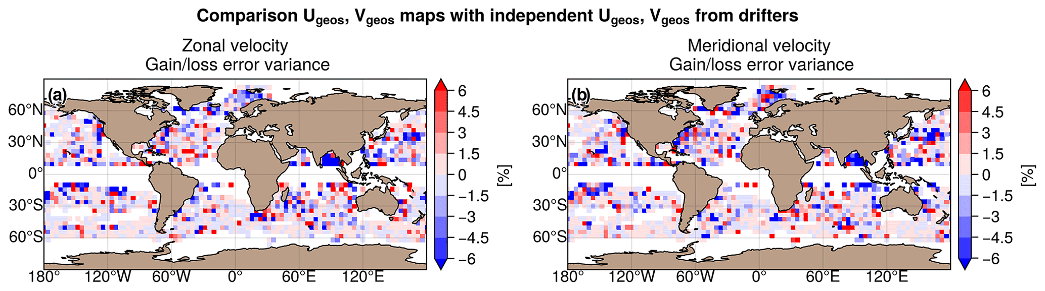
Figure 11 Gain/loss of the mapping error variance of currents in the MIOST allsat-1 80 % drifters + equatorial waves + L3 Arctic experiment relative to the MIOST allsat-1 mapping error variance for (c) the zonal velocity component and (d) the meridional velocity component. Blue colour means a reduction of error in MIOST when drifters are included in the mapping and with equatorial wave parametrization.

Table 7 Regionally averaged mapping error variance and gain/reduction of error variance on the surface currents between MIOST allsat-1 and MIOST allsat-1 80 % drifters + equatorial waves + L3 Arctic.

4.2.3 Overall assessment

The comparison of the MIOST allsat-1 80 % drifters + equatorial waves + L3 Arctic and DUACS allsat-1 experiments allows the complete MIOST product distributed to users to be evaluated against the DUACS method.

Sea-level anomaly quality

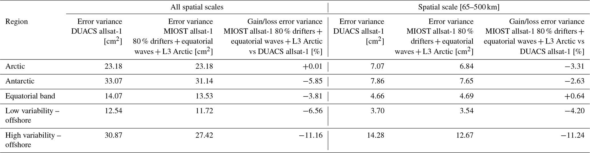
The differences in mapping error between MIOST allsat-1 80 % drifters + equatorial waves + L3 Arctic and DUACS allsat-1 are shown in Fig. 12a and b for all spatial scales and the spatial scale between 65 and 500 km, respectively. We have the same pattern as found in the previous sections: for all spatial scales considered (Fig. 12a), the equatorial wave modes help to reduce the mapping error variance in the equatorial band by more than 20 % locally. At mid-latitudes, the mapping error is between 5 % and 10 % smaller with MIOST than with DUACS. For spatial scales between 65 and 500 km, MIOST and DUACS solutions are globally equivalent, except in the high-variability region where the mapping error is between 10 % and 20 % smaller with MIOST than with DUACS. The mapping errors are locally larger with MIOST than with DUACS in regions where the circulation interacts with bathymetry features such as in the Argentine Sea and near the Siberian plateau and New Zealand plateau. Table 8 summarizes the results of the comparison over different regions of interest: mapping errors are ∼ 11 % smaller in high-variability regions in MIOST than in DUACS. In other regions, the errors are ∼ 3 %–6 % smaller.

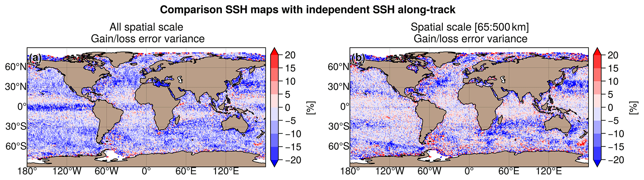
Figure 12 Gain/loss of the mapping error variance of SLA in the MIOST allsat-1 80 % drifters + equatorial waves + L3 Arctic experiment relative to the DUACS allsat-1 mapping error variance for (a) all spatial scales and (b) the scale between 65 and 500 km. Blue colour means a reduction of error variance in MIOST.

Table 8 Regionally averaged mapping error variance and gain/reduction of error variance on the SSH variable between MIOST allsat-1 80 % drifters + equatorial waves + L3 Arctic and DUACS allsat-1.

Geostrophic current quality

The differences in mapping error of surface geostrophic currents between MIOST allsat-1 80 % drifters + equatorial waves + L3 Arctic and DUACS allsat-1 are shown in Fig. 13a and b for the zonal component and the meridional component of the velocity, respectively. The mapping errors are globally smaller in MIOST than in DUACS, particularly in the high-variability regions. In the tropical regions, DUACS outperforms MIOST for reconstructing the surface geostrophic velocities. Overall, the mapping errors are on average between ∼ 2 % and 5 % smaller with MIOST than with DUACS (Table 9).

Figure 13 Gain/loss of the mapping error variance of currents in the MIOST allsat-1 80 % drifters + equatorial waves + L3 Arctic experiment relative to the DUACS allsat-1 mapping error variance for (c) the zonal velocity component and (d) the meridional velocity component. Blue colour means a reduction of error in MIOST.

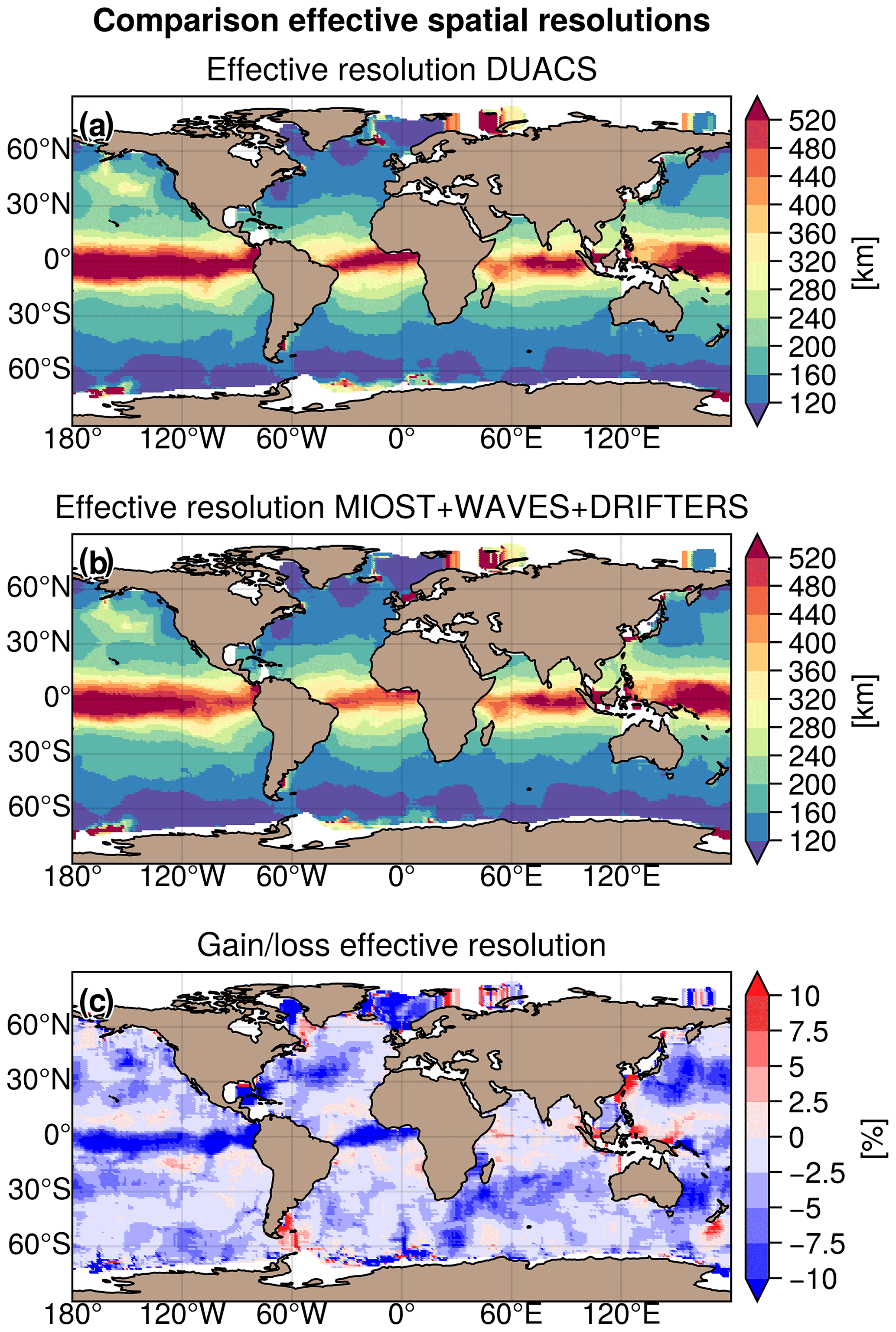
Figure 14 Maps of effective spatial resolution (in km) for (a) the DUACS allsat-1 and (b) MIOST allsat-1 80 % drifters + equatorial waves + L3 Arctic experiments and (c) gain/loss of effective resolution (in %) between MIOST and DUACS. Blue means finer resolution in MIOST than in DUACS.

Table 9 Regionally averaged mapping error variance and gain/reduction of error variance on the surface currents between MIOST allsat-1 80 % drifters + equatorial waves + L3 Arctic and DUACS allsat-1.

Effective resolution

The effective spatial resolution quantifies the minimum spatial scale resolved in the maps (Ballarotta et al., 2019). Maps of the effective spatial resolution (expressed in kilometres) are presented in Fig. 14a and b for DUACS allsat-1 and MIOST allsat-1 80 % drifters + equatorial waves + L3 Arctic, respectively. For each experiment, the effective spatial resolution varies from ∼ 500 km at the Equator to ∼ 100 km at high latitudes and a mean value at mid-latitudes close to 200 km. The difference in effective spatial resolution between the two experiments is shown in Fig. 14c. The resolution of the SLA maps of the MIOST experiment is overall finer than in the SLA maps of the DUACS experiment. It is between 5 % and 10 % finer than the DUACS maps in regions of high variability (the Gulf Stream, Kuroshio, and Agulhas regions), in the Atlantic and equatorial Pacific, and in the Norwegian and Greenland seas. Some regions (e.g. tropical regions, coastal regions, the East China Sea, the New Zealand Shelf, or the Argentine Sea) are subject to a coarser effective resolution in MIOST maps than in DUACS maps. These regions will require further investigation in the near future.

5 Data availability

The MIOST gridded products are hosted on the AVISO+ (Archivage, Validation et Interprétation des données des Satellites Océanographiques) website (https://doi.org/10.24400/527896/a01-2022.009, Ballarotta et al., 2022).

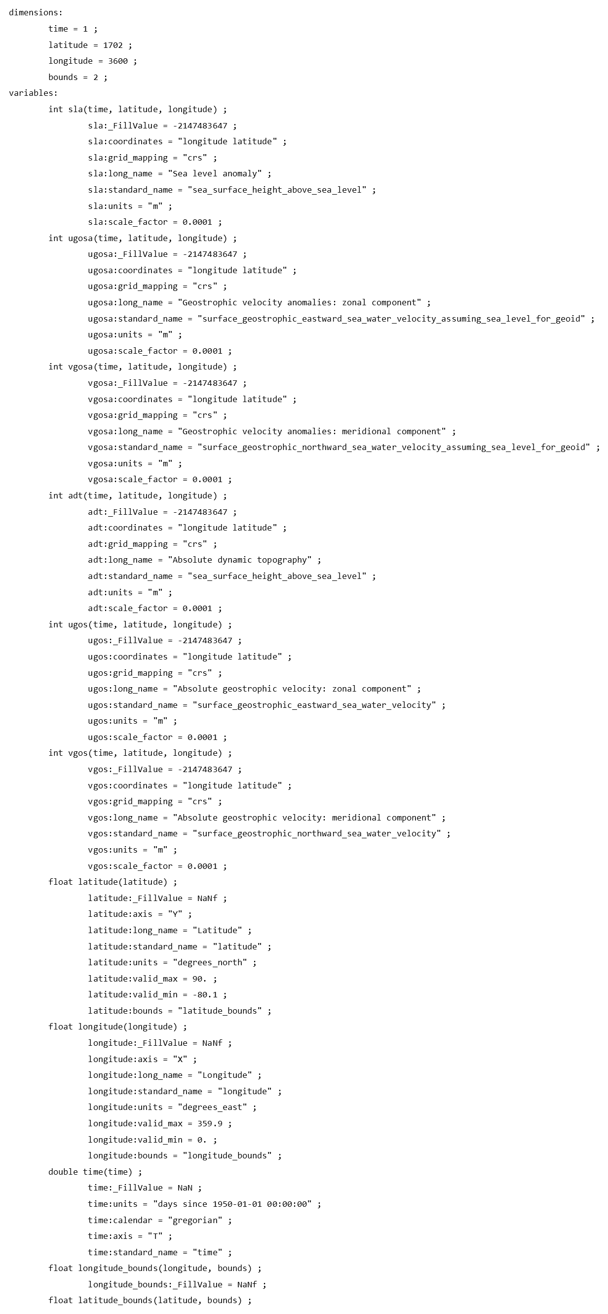
The reference DUACS maps are hosted on the EU Copernicus Marine Service portal (https://doi.org/10.48670/moi-00148, Pujol et al., 2022b). The multiscale and multivariate products are distributed on a regular grid: the spatial grid extends from 0 to 360^∘ E in longitude and 80^∘ S to 90^∘ N in latitude, with a grid spacing of 0.1^∘; the temporal grid covers the period 1 July 2016 to 30 June 2020 with a time step of 1 d. The dataset is distributed in netCDF4 format. Each netCDF file contains six variables: sla, adt, ugosa,vgosa, ugos, and vgos (see the list of variables available in the MIOST product in Fig. 15).

Figure 15 List of variables available in the multiscale and multivariate product.

6 Summary and conclusions

Ubelmann et al. (2021, 2022) evaluated the multiscale and multivariate mapping approach in the Observing System Simulation Experiment (OSSE) and the Observing System Experiment (OSE) for the simultaneous mapping of mesoscale circulation, coherent internal tides, and surface geostrophic and ageostrophic velocities. Here, we extend the application of the MIOST solution to the simultaneous mapping of equatorial waves and mesoscale circulation from real observations. Furthermore, we investigate the levels of mapping improvement by enhancing the sampling of the ocean surface state with in situ data and altimetry data in the Arctic sea-ice regions. We found that the Arctic lead SSH observations allow the monitoring coverage in this remote region to be significantly improved. The gap-free maps, proposed with MIOST, hence offer the opportunity to end users to study the Arctic surface circulation and its connections to the subpolar and mid-latitude regions. It is important to mention that this polar mapping will need to be validated against independent data in the near future. Drifters' observations have a moderate impact in the mapping. They mainly contribute to reduce mapping errors in regions of intense dynamics where the temporal sampling must be accurate enough to properly map the rapid mesoscale dynamics. It is important note that drifter observations can potentially improve surface circulation in areas not or poorly sampled by altimeters. Therefore, their impact on the sea-level reconstruction may be larger over periods of weak altimeter sampling.

The ocean surface circulation involves a superposition of processes acting at widely different spatial and temporal scales, from the geostrophic large-scale and slow-varying flow to the mesoscale turbulent eddies and, at even smaller scales, the mixing generated by the internal wave field. It is also important to mention that the DUACS maps are constructed from altimetry data using an interpolation method optimized for mapping mesoscale variability. Consequently, some ocean surface variabilities are not or poorly represented in these DUACS maps: equatorial wave dynamics is thus part of the filtered ocean signals in DUACS. The multiscale approach allows the observed SSH to be decomposed into various physical contributions. Here, we explored and validated the possibility of improving the content of altimetry maps by simultaneously estimating the ocean mesoscale circulations as well as the equatorial wave dynamics associated with the tropical instability waves and Poincaré waves. We show that mapping these ocean surface variabilities from altimeter observations broadens the spectrum of mappable space–timescales and reduces mapping errors by almost 20 % locally relative to independent data, primarily in the equatorial Pacific and Atlantic basins. This is possible because the spatio-temporal coverage of the altimeter data allows large-scale waves of 4 d periods and longer to be sampled. At global scale, we also found that, compared to the operational DUACS mapping approach, MIOST approach improves the surface mesoscale circulations in regions of high variability. Consequently, the effective resolution of the maps produced by the multiscale approach is finer than the DUACS maps, particularly in the western boundary currents and in the equatorial band.

This experimental product is currently available on the AVISO + (Archivage, Validation et Interprétation des données des Satellites Océanographiques) website (see the “Data availability” section for more details), but our results suggest that the multiscale and multivariate mapping approach is very promising for use in an operational context. It is also worth mentioning that several other global gridded products exist as an alternative to the DUACS/MIOST products which provide only the geostrophic part of the surface current. Examples of these other products that provide a broader spectrum of ocean surface current variability (e.g. the total surface currents) include (1) the Copernicus GLORYS12v1 global ocean reanalysis (Lellouche et al., 2018; https://doi.org/10.48670/moi-00021, Drévillon et al., 2022), (2) the Copernicus GLOBCURRENT product (Rio et al., 2014; https://doi.org/10.48670/moi-00050, Etienne, 2021b), or (3) the OSCAR product (Dohan, 2021; https://doi.org/10.5067/OSCAR-25F20 Dohan, 2021) distributed by the NASA-JPL Distributed Physical Oceanography Active Archive Center (PO. DAAC).

To conclude, these results pave the way for the exploration of new types of ocean signals that may eventually be mapped with MIOST from remote sensing and in situ observations. Future work could consist of enriching the MIOST components in considering oceanic signals missing in the maps and yet captured by observing systems: for example, in mapping high-frequency signals such as the near-inertial oscillation from drifter observations, in using SSH lead products in the Southern Ocean (Auger et al., 2022), or by enhancing the SLA map content with a dynamical model approach (Ubelmann et al., 2015) or artificial intelligence methods (Beauchamp et al., 2020).

Appendix A: Mapping approaches tested in this study

A1 The optimal interpolation (DUACS mapping approach)

The DUACS mapping approach constructs a SSH field on a regular grid by combining measurements from various altimeters. It is based on a global suboptimal space–time objective analysis that considers along-track correlated errors as described, for instance, in Ducet et al. (2000) or Le Traon et al. (2003). The mathematical formulation, known as optimal interpolation, is described hereafter.

We assume a state to estimate, denoted x, and partial observations, denoted y, which can be related to the state by a linear operator H such as

$$\begin{array}{}\text{(A1)}& y=Hx+\mathit{ϵ},\end{array}$$

where ϵ is an independent signal (e.g. observation error) not related to the state. If we define B the covariance matrix of x and R the covariance matrix of ϵ, both variables being assumed Gaussian, then the linear estimate is written as

$$\begin{array}{}\text{(A2)}& {\mathit{x}}^{\mathrm{a}}=\mathbf{B}{H}^{\mathrm{T}}{\left(H\mathbf{B}{H}^{\mathrm{T}}-\mathbf{R}\right)}^{-\mathrm{1}}\mathit{y}.\end{array}$$

The observation vector y represents the SLA observations. The state vector x is the gridded SLA. The operator H (formally a trilinear interpolator transforming the gridded state SLA to the equivalent along-track SLA) is not considered explicitly. The matrices BH^T and HBH^T, representing the covariance of the signal in the (grid, obs) and (obs, obs) spaces, are directly written with the analytical formula of the Arhan and Colin de Verdière (1985) covariance model as described in Ducet et al. (2000), Le Traon et al. (2003), or Pujol et al. (2016):

$$\begin{array}{}\text{(A3)}& {\displaystyle }C\left(x,y,t\right)=\left(\mathrm{1}+\mathrm{ar}+{\displaystyle \frac{\mathrm{1}}{\mathrm{6}}}(\mathrm{ar}{)}^{\mathrm{2}}-{\displaystyle \frac{\mathrm{1}}{\mathrm{6}}}(\mathrm{ar}{)}^{\mathrm{3}}\right)e^{-\mathrm{ar}}{e}^{-{\left(\frac{t}{L_t}\right)}^{\mathrm{2}}}\text{(A4)}& {\displaystyle }r=\sqrt{{\left({\displaystyle \frac{x-C_{\mathrm{px}}t}{L_x}}\right)}^{\mathrm{2}}+{\left({\displaystyle \frac{y-C_{\mathrm{py}}t}{L_y}}\right)}^{\mathrm{2}}},\end{array}$$

where, x, y, and t correspond to the zonal, meridional, and temporal position; L_x, L_y, and L_t are the zonal, meridional, and temporal decorrelation scale; C_px and C_py denote the phase speed; and a is a constant (3.337).

This covariance model is mainly optimized for mesoscale signal reconstruction. The R matrix represents the representativity and instrumental errors. Since the covariance of mesoscale SLA is assumed to vanish beyond a few hundreds of kilometres in space and beyond 10–20 d in time (Le Traon and Dibarboure, 2002), separate inversions are performed locally, selecting observations over time and space windows adjusted to these values. In practice, since the number of observations is limited to less than 1000 (Le Traon et al., 1998), the inversion in observation space is computationally manageable. More details on the map production are given in Pujol et al. (2016).

In DUACS, the geostrophic current (U_g, V_g) is then directly derived from the mapped SSH:

$$\begin{array}{}\text{(A5)}& {\displaystyle }{U}_{\mathrm{g}}\left(x,y\right)=-{\displaystyle \frac{g}{f_{\mathrm{c}}}}{\displaystyle \frac{\partial \mathrm{SSH}\left(x,y\right)}{\partial y}}\text{(A6)}& {\displaystyle }{V}_{\mathrm{g}}\left(x,y\right)={\displaystyle \frac{g}{f_{\mathrm{c}}}}{\displaystyle \frac{\partial \mathrm{SSH}\left(x,y\right)}{\partial x}},\end{array}$$

where g is the gravity, and f_c is the Coriolis frequency, which is a function of latitude.

A2 A multiscale and multivariate mapping approach

The optimal interpolation requires the inversion of a matrix of the same size as the observation vector y. When the number of observations exceeds the size of the state to resolve, it can be interesting to use an equivalent formulation given by the Sherman–Morrison–Woodbury transformation, allowing for an inversion in state space, with a matrix of the size of the state vector x:

$$\begin{array}{}\text{(A7)}& {\mathit{x}}^{\mathrm{a}}=(H^{\mathrm{T}}\textcolor{red}{}{\mathbf{R}}^{-\mathrm{1}}H+{\mathbf{B}}^{-\mathrm{1}})\textcolor{red}{}{H}^{\mathrm{T}}{\mathbf{R}}^{-\mathrm{1}}\mathit{y}.\end{array}$$

The formulation of the multiscale and multivariate mapping algorithm is detailed in Ubelmann et al. (2022). Here we recall the main principle. We consider an extended state vector × composed by N physical components that will later be assumed independent. In this study N=3 for (1) geostrophy and equatorial waves, (2) tropical instability waves (TIWs), and (3) Poincaré waves:

$$\begin{array}{}\text{(A8)}& x={\left(x_{\mathrm{1}}^{\mathrm{T}},\mathrm{\dots },x_N^{\mathrm{T}}\right)}^{\mathrm{T}}.\end{array}$$

Each component x_k represents the state of the surface topography and surface current to be resolved in the grid space, denoted $x_k={\left(h_k^{\mathrm{T}},u_k^{\mathrm{T}},v_k^{\mathrm{T}}\right)}^{\mathrm{T}}$. The key aspect of the method is a rank reduction of the state vector, through a subcomponent decomposition, such as x_k, which can be written as

$$\begin{array}{}\text{(A9)}& x_k=\left[\begin{array}{l}{\mathbf{\Gamma }}_{k,h}\\ {\mathbf{\Gamma }}_{k,u}\\ {\mathbf{\Gamma }}_{k,v}\end{array}\right]{\mathit{\eta }}_k={\mathbf{\Gamma }}_k{\mathit{\eta }}_k,\end{array}$$

where η_k is the reduced state vector for component k, and Γ_k,h, Γ_k,u, and Γ_k,v are the subcomponent matrices expressed in topography and currents, respectively. Note that for some components, one of the blocks can be set to zeros (e.g. if the geostrophy component is considered to have zero contribution to SSH, which is the case for the equatorial wave components). Their concatenation is called Γ_k, which is the matrix transforming the reduced state vector in the grid space for topography and currents. In practice, Γ_k will be a wavelet decomposition of the time–space domain, with elements of appropriate temporal and spatial scales to represent the component k. These wavelet scales, and their specified variance set with a diagonal matrix noted Q_k, will define the equivalent covariance model B_k in the grid space for component k:

$$\begin{array}{}\text{(A10)}& B_k={\mathbf{\Gamma }}_k{\mathbf{Q}}_k{\mathbf{\Gamma }}_k^{\mathrm{T}}.\end{array}$$

The observation vector y is also extended to the observed surface topography and surface current noted $y={\left(h^{\mathrm{oT}},u_r^{\mathrm{oT}}\right)}^{\mathrm{T}}$. Then, if H_k is the observation operator for component k (from grid space to observation space), we note G_k= H_k Γ_k, the subcomponent matrix expressed in observation space. In these conditions, the observation vector y is the sum of all component contributions plus the unexplained signal ϵ (instrument error and representativity):

$$\begin{array}{}\text{(A11)}& \mathit{y}=\sum _{k=\mathrm{1}}^N{G}_k{\mathit{\eta }}_k+\mathit{ϵ}.\end{array}$$

If we use the notation $\mathit{\eta }={\left({\mathit{\eta }}_{\mathrm{1}}^{\mathrm{T}},\mathrm{\dots },{\mathit{\eta }}_k^{\mathrm{T}}\right)}^{\mathrm{T}}$ for the concatenation of the subcomponent state vectors, and $G=(G_{\mathrm{1}},\mathrm{\dots },G_N$), then we have

$$\begin{array}{}\text{(A12)}& y=G\mathit{\eta }+\mathit{ϵ}.\end{array}$$

Applying the same transformation from Eqs. (A1), (A2), and (A7) to the reduced state vector η, the global solution is written as

$$\begin{array}{}\text{(A13)}& {\mathit{\eta }}^{\mathrm{a}}={\left(G^{\mathrm{T}}{\mathbf{R}}^{-\mathrm{1}}G+{\mathbf{Q}}^{-\mathrm{1}}\right)}^{-\mathrm{1}}{G}^{\mathrm{T}}{R}^{-\mathrm{1}}y,\end{array}$$

where Q is the covariance matrix of η, expressed as the concatenation of the diagonal matrices Q_k for each component. Finally, the solution in the reduced-space projects into the grid space with the following relation:

$$\begin{array}{}\text{(A14)}& x_{\mathrm{a}}=\mathbf{\Gamma }{\mathit{\eta }}^{\mathrm{a}}.\end{array}$$

In practice, to solve Eq. (A13), each block of G is directly filled from the analytical expression of the reduced-space elements constituting the columns of the matrix. Also, in many situations, the $\left(G^{\mathrm{T}}{R}^{-\mathrm{1}}G+Q^{-\mathrm{1}}\right)$ matrix, noted A hereafter, would be too large to be inverted (as required by Eq. A13 explicitly). We use a preconditioned conjugate gradient method to solve $\mathit{\eta }=A^{-\mathrm{1}}z$, where $z=G^{\mathrm{T}}{\mathbf{R}}^{-\mathrm{1}}y$ is computed initially from G and the observation vector y. The algorithm involves many iterations of Aη computations for updated η until convergence is reached (when Aη approaches z). Note that if A is too large to be written explicitly, the result Aη can still be computed in two steps from a matrix multiplication of G and then of G^T. Once the solution η is obtained, the projection in physical grid space given by Eq. (A14) is applied sequentially, by summing the analytical expression of the ripples applied to grid coordinates (the columns of Γ), separately for each component k. As in any inversion based on linear analysis, the result strongly relies on the choice of covariance models, here defined by the reduced elements of each component.

A2.1 Geostrophy component

Geostrophy is the component that has a signature on both topography and currents and on which some synergy between altimetry and drifter observations can be expected. Following the formulation provided in Ubelmann et al. (2021), here we define the gridded variable H₁ to resolve, and the corresponding gridded geostrophic current field (U₁, V₁) is written

$$\begin{array}{}\text{(A15)}& \left\{\begin{array}{l}{U}_{\mathrm{1}}=-\frac{g}{f_{\mathrm{c}}}\frac{\partial H_{\mathrm{1}}}{\partial y}\\ V_{\mathrm{1}}=\frac{g}{f_{\mathrm{c}}}\frac{\partial H_{\mathrm{1}}}{\mathrm{d}x}.\end{array}\right.\end{array}$$

The proposed reduced state for geostrophy is based on an element decomposition of H₁, expressed by Γ_1,h with wavelets of various wavelength and temporal extensions. This will allow the standard covariance models used in altimetry mapping to be approximated, accounting for specific variations with wavelength and time. A given p element of the decomposition Γ_1,h is expressed as follows:

$$\begin{array}{}\text{(A16)}& \begin{array}{rl}{\mathbf{\Gamma }}_{\mathrm{1},h}\left[i,p\right]& =\cos \left(k_{x,\mathrm{p}}\left(x_i-x_{\mathrm{p}}\right)+k_{y,\mathrm{p}}\left(y_i-y_{\mathrm{p}}\right)+{\mathrm{\Phi }}_{\mathrm{p}}\right)\\ & \times f_{\mathrm{tap}}\left({\displaystyle \frac{x_i-x_{\mathrm{p}}}{L_{x_{\mathrm{p}}}}},{\displaystyle \frac{y_i-y_{\mathrm{p}}}{L_{y_{\mathrm{p}}}}},{\displaystyle \frac{t_i-t_{\mathrm{p}}}{L_{t_{\mathrm{p}}}}}\right),\end{array}\end{array}$$

where the ith line of the matrix stands for a given grid index of coordinates (x_i, y_i, t_i). For the ensemble of p, Φ_p is alternatively 0 and $\mathit{\pi }/\mathrm{2}$, such that all subcomponents are defined by pairs of sine and cosine functions to allow for the phase degree of freedom. k_x,p and k_y,p are zonal and meridional wavenumbers respectively, set to vary in the mappable mesoscale range (between 80 and 900 km with a spacing inversely proportional to the wavelet extensions, allowing a signal of any intermediate wavelength to be represented). (x_p, y_p, t_p) are the coordinates of a space–time pavement. The function f_tap localizes the subcomponent in time and space (at scales $L_{t_{\mathrm{p}}}$ , $L_{x_{\mathrm{p}}}$, and $L_{y_{\mathrm{p}}}$, respectively) as geostrophy has a local extension of covariances. It is expressed as

$$\begin{array}{}\text{(A17)}& \begin{array}{rl}& f_{\mathrm{tap}}\left(\mathit{\delta }x,\mathit{\delta }y,\mathit{\delta }t\right)\\ & =\left\{\begin{array}{ll}\cos \left(\frac{\mathit{\pi }}{\mathrm{2}}\mathit{\delta }x\right)\cos \left(\frac{\mathit{\pi }}{\mathrm{2}}\mathit{\delta }y\right)\cos \left(\frac{\mathit{\pi }}{\mathrm{2}}\mathit{\delta }y\right),& \text{for}\left(\left|\mathit{\delta }x\right|,\left|\mathit{\delta }y\right|,\left|\mathit{\delta }y\right|\right.\\ & \left.<\left(\mathrm{1},\mathrm{1},\mathrm{1}\right)\right)\\ \mathrm{0},& \text{elsewhere.}\end{array}\right.\end{array}\end{array}$$

In practice, $L_{x_{\mathrm{p}}}$ and $L_{y_{\mathrm{p}}}$ will be set to 1.5 the wavelength of element p and $L_{t_{\mathrm{p}}}$ to the decorrelation timescale. Then, the same element p of the decomposition also has an expression in the geostrophic current (through the geostrophic relation Eq. A15) written in the Γ_1,u and Γ_1,v matrices:

$$\begin{array}{}\text{(A18)}& \left\{\begin{array}{l}{\mathbf{\Gamma }}_{\mathrm{1},u}\left[i,p\right]=-\frac{g}{f_{\mathrm{c}}}\frac{\partial {\mathbf{\Gamma }}_{\mathrm{1},h}\left[i,p\right]}{\partial y_i}\\ {\mathbf{\Gamma }}_{\mathrm{1},v}\left[i,p\right]=\frac{g}{f_{\mathrm{c}}}\frac{\partial {\mathbf{\Gamma }}_{\mathrm{1},h}\left[i,p\right]}{\partial x_i}.\end{array}\right.\end{array}$$

The whole time–space domain is paved with similar subcomponents, along coordinates (x_p, y_p, t_p) for wavelengths between 80 and 900 km spanning in all directions of the plan. The ensemble can be seen as a wavelet basis. Finally, each subcomponent p is assigned an expected variance in the Q₁ matrix, consistent with the power spectrum observed from altimetry at the corresponding wavelength with isotropy assumption.

A2.2 Equatorial wave component

Here we define the gridded variables H₂ and H₃ to resolve TIW and Poincaré waves, respectively, and we consider no contributions of the equatorial wave components to the geostrophic currents; therefore the corresponding gridded geostrophic current fields (U₂, V₂) and (U₃, V₃) are written $U_{\mathrm{2}}=U_{\mathrm{3}}=$0, $V_{\mathrm{2}}=V_{\mathrm{3}}=$0. The reduced state is represented in the time–space domain by the following Γ_2,h and Γ_3,h matrix:

$$\begin{array}{}\text{(A19)}& {\displaystyle }\begin{array}{rl}{\mathbf{\Gamma }}_{\mathrm{2},h}\left[i,p\right]& =\cos \left({\mathit{\omega }}_{\mathrm{2},t,\mathrm{p}}\left(t_i-t_{\mathrm{p}}\right)-k_{\mathrm{2},x,\mathrm{p}}\left(x_i-x_{\mathrm{p}}\right)\right)\\ & \times f_{\mathrm{tap}}\left({\displaystyle \frac{x_i-x_{\mathrm{p}}}{L_{\mathrm{2},x_{\mathrm{p}}}}},{\displaystyle \frac{y_i-y_{\mathrm{p}}}{L_{\mathrm{2},y_{\mathrm{p}}}}},{\displaystyle \frac{t_i-t_{\mathrm{p}}}{L_{\mathrm{2},t_{\mathrm{p}}}}}\right)\end{array}\text{(A20)}& {\displaystyle }\begin{array}{rl}{\mathbf{\Gamma }}_{\mathrm{3},h}\left[i,p\right]& =\cos \left({\mathit{\omega }}_{\mathrm{3},t,\mathrm{p}}\left(t_i-t_{\mathrm{p}}\right)-k_{\mathrm{3},x,\mathrm{p}}\left(x_i-x_{\mathrm{p}}\right)\right)\\ & \times f_{\mathrm{tap}}\left({\displaystyle \frac{x_i-x_{\mathrm{p}}}{L_{\mathrm{3},x_{\mathrm{p}}}}},{\displaystyle \frac{y_i-y_{\mathrm{p}}}{L_{\mathrm{3},y_{\mathrm{p}}}}},{\displaystyle \frac{t_i-t_{\mathrm{p}}}{L_{\mathrm{3},t_{\mathrm{p}}}}}\right),\end{array}\end{array}$$

where $k_{\mathrm{2},x,\mathrm{p}}$ and $k_{\mathrm{3},x,\mathrm{p}}$ refer to the zonal wavenumber, and ${\mathit{\omega }}_{\mathrm{2},t,\mathrm{p}}$ and ${\mathit{\omega }}_{\mathrm{3},t,\mathrm{p}}$ are the frequency which satisfies the dispersion relation of the wave component (Matsuno, 1966); for example,

$$\begin{array}{}\text{(A21)}& \left\{\begin{array}{l}{\mathit{\omega }}_{\mathrm{2},t,\mathrm{p}}=c_{\mathrm{2}}\cdot k_{\mathrm{2},x,\mathrm{p}}\text{for the TIW},c_{\mathrm{2}}=-\mathrm{0.5}\mathrm{m}{\mathrm{s}}^{-\mathrm{1}}\\ {\mathit{\omega }}_{\mathrm{3},t,\mathrm{p}}=\sqrt{k_{\mathrm{3},k,\mathrm{p}}^{\mathrm{2}}\cdot c_{\mathrm{3}}^{\mathrm{2}}+\mathit{\beta }\cdot c_{\mathrm{3}}\cdot \left(\mathrm{2}\cdot n+\mathrm{1}\right)}\\ \text{for the Poincaré waves},c_{\mathrm{3}}=\pm \mathrm{2.8}\mathrm{m}{\mathrm{s}}^{-\mathrm{1}},\end{array}\right.\end{array}$$

where c₂ and c₃ denote the wave propagation speed (the sign indicating the direction of propagation, negative for westward and positive for eastward), β is the meridional gradient of the Coriolis frequency f_c, and $n=\mathrm{1},\mathrm{2},\mathrm{3}\mathrm{\dots }$

In the present study, we chose $L_{\mathrm{2},t_{\mathrm{p}}}=\mathrm{20}$ d, $L_{\mathrm{2},x_{\mathrm{p}}}=\mathrm{500}$ km, and $L_{\mathrm{2},y_{\mathrm{p}}}=\mathrm{300}$ km for the TIW component and $L_{\mathrm{3},t_{\mathrm{p}}}=\mathrm{5}$ d, $L_{\mathrm{3},x_{\mathrm{p}}}=$1000 km, and $L_{\mathrm{3},y_{\mathrm{p}}}=\mathrm{300}$ km for the equatorial Poincaré wave component. As for the geostrophy component, the function f_tap localizes the subcomponent in time and space (at scales $L_{t_{\mathrm{p}}}$ , $L_{x_{\mathrm{p}}}$, and $L_{y_{\mathrm{p}}}$, respectively).