the Creative Commons Attribution 4.0 License.
the Creative Commons Attribution 4.0 License.
 | 06 Jul 2023
High-frequency, year-round time series of the carbonate chemistry in a high-Arctic fjord (Svalbard)
Jean-Pierre Gattuso
Samir Alliouane
Philipp Fischer
The Arctic Ocean is subject to high rates of ocean warming and acidification, with critical implications for marine organisms as well as ecosystems and the services they provide. Carbonate system data in the Arctic realm are spotty in space and time, and, until recently, there was no time-series station measuring the carbonate chemistry at high frequency in this region, particularly in coastal waters. We report here on the first high-frequency (1 h), multi-year (5 years) dataset of salinity, temperature, CO2 partial pressure (pCO2) and pH at a coastal site (bottom depth of 12 m) in a high-Arctic fjord (Kongsfjorden, Svalbard). Discrete measurements of dissolved inorganic carbon and total alkalinity were also performed. We show that (1) the choice of formulations for calculating the dissociation constants of the carbonic acid remains unsettled for polar waters, (2) the water column is generally somewhat stratified despite the shallow depth, (3) the saturation state of calcium carbonate is subject to large seasonal changes but never reaches undersaturation (Ωa ranges between 1.4 and 3.0) and (4) pCO2 is lower than atmospheric CO2 at all seasons, making this site a sink for atmospheric CO2 (−9 to −16.8 , depending on the parameterisation of the gas transfer velocity). Data are available on PANGAEA: https://doi.org/10.1594/PANGAEA.960131 (Gattuso et al., 2023a).
- Article
(3362 KB) - Full-text XML
- BibTeX
- EndNote


Despite their major importance, Arctic shelves are among the coastal areas which are understood the least. The Arctic Ocean only covers 4.3 % of the total ocean area but has a continental shelf considerably larger than other oceans (52.7 % of its total area vs. less than 18 % globally; Jakobsson et al., 2004; Menard and Smith, 1966), and the total length of its coastline affected by the presence of permafrost represents around 34 % of the world's coastline (Lantuit et al., 2012). It contains less than 1 % of global ocean water but receives 11 % of the global runoff (Shiklomanov, 1998) and is responsible for 7 %–10 % of the global burial of organic carbon (Stein and Macdonald, 2004).
The Arctic region is one of the “reasons for concern” of the Intergovernmental Panel on Climate Change (IPCC; O'Neill et al., 2017). The Arctic Ocean exhibits the fastest and largest changes which already have impacts on the biota and biogeochemical cycles (Wassmann et al., 2010). The increase in sea surface temperature over the last 2 decades is similar to (or only slightly higher than) the global average (Fox-Kemper et al., 2021) . However, the greatest future warming is in the Arctic Ocean, where multi-model mean warming during 2080–2099 can exceed 2 to 5 ∘C relative to 1995–2014, depending on the CO2 emissions scenario considered (Kwiatkowski et al., 2020).
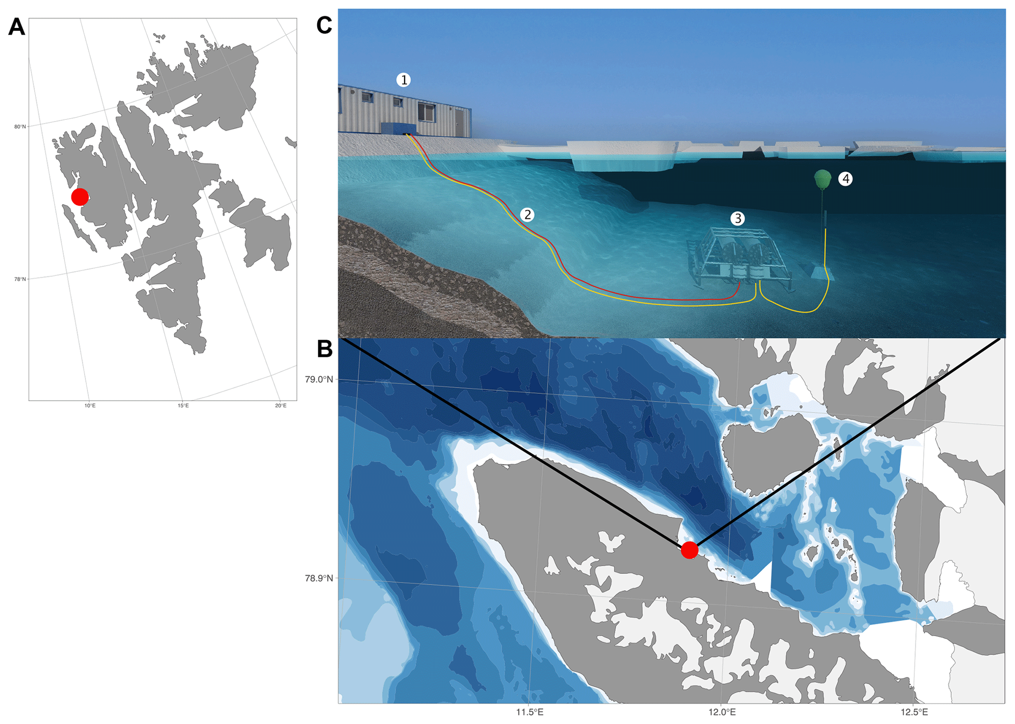
Figure 1Svalbard (a), Kongsfjorden and Ny-Ålesund (b), and observational set-up (c). 1: FerryBox system, 2: underwater cable and underwater tubes for the water supply for FerryBox system, 3: underwater node with water pumps, 4: underwater profiling sensor carrier unit (REMOS, Remote Operated Observing System). The maps were produced by the R package ggOceanMaps (Vihtakari, 2022).
The massive release of anthropogenic CO2 also generates ocean acidification, a process that describes the increase in dissolved inorganic carbon and bicarbonate as well as the decline of pH and the saturation state of calcium carbonate minerals. The decrease in pH is projected to be larger in the surface Arctic Ocean than elsewhere, with model mean declines that can exceed 0.45 pH units in SSP5-8.5 (2080–2099 anomalies relative to 1995–2014) (Kwiatkowski et al., 2020).
Freshwater input via rivers and glacier melting has a profound impact on the seawater carbonate chemistry. It decreases total alkalinity, the seawater buffering capacity and the calcium carbonate saturation state (Fransson et al., 2015). Undersaturation of surface water with respect to aragonite-type CaCO3 was first reported in 2008 for the Canada Basin, preceding other open-ocean basins (Zhang et al., 2020). Much of Arctic shallow waters are undersaturated with respect to calcium carbonate, especially aragonite. This is due to the decrease of salinity resulting from increased river runoff and sea-ice melt in the summer (Chierici and Fransson, 2009) and to the degradation of organic matter in runoff waters and shelf areas (e.g. Anderson et al., 2017). Aragonite undersaturation has consequences for aragonite-shelled organisms such as pteropods (e.g. Comeau et al., 2011).
The remoteness and harsh environmental conditions make it difficult to gather carbonate chemistry data in the Arctic, although some coastal sites are easily accessible year round. The goal of this paper is to provide the first high-frequency, multi-year dataset of salinity, temperature, dissolved inorganic carbon, total alkalinity, pCO2 and pH.
Data were collected at the COSYNA/MOSES-AWIPEV underwater observatory operated since 2012 in Kongsfjorden, an Arctic fjord located on the west coast of Spitsbergen (Svalbard) at 78∘55′50.37′′ N, 11∘55′12.10′′ E (Fischer et al., 2017) (Fig. 1). The study site is coastal (11 m depth ± 0.7 m of tidal amplitude) and is relatively sheltered in the inner part of Kongsfjorden, with average tidal currents of 0.1 m yr−1. Kongsfjorden is a typical Arctic fjord with minimum winter water temperatures of −1.9 to 0.8 ∘C in February and March and maximum average water temperatures of more than 6 ∘C in August (see Appendix A). Until 2006, the fjord was regularly covered by sea ice in winter (Gerland and Renner, 2007). Before 2006, the sea ice typically extended into the central part of the fjord, but during the last decade the sea-ice extent has often been reduced to the northern part of the inner bay (Pavlova et al., 2019).
Table 1Sensors deployed in the FerryBox and profiling systems. All sensors in the FerryBox system are maintained once a year, and all sensors of the profiling system are changed once a year and sent to the manufacturer for maintenance and calibration. The salinity sensors were calibrated according to the standard UNESCO procedure (IOC et al., 2010). FTU represents Formazin Turbidity Units.
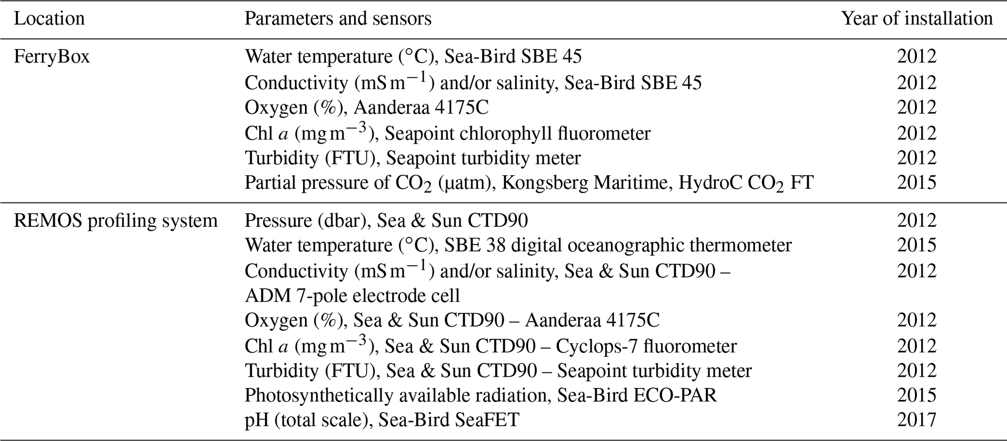
Calculated according to the salinity standard UNESCO procedures (IOC et al., 2010).
2.1 The COSYNA/MOSES-AWIPEV observatory
The COSYNA/MOSES-AWIPEV underwater observatory comprises a land-based FerryBox system (Fig. 1a) equipped with a set of sensors (Table 1). The FerryBox receives water from 11 m depth from an underwater pump (Fig. 1b and c). To prevent biofouling of the sensors, every night at 00:05 UTC a sulfuric acid (4 % for 15 min) flush of the entire sensor system was followed by a rinse with freshwater (30 min) prior to switching again to measuring mode. Data were not used for a total duration of 60 min after the initiation of the flush. The observatory also comprises a profiling sensor carrier (REMOS) fitted with another set of sensors that can be remotely controlled (Fig. 1c (label 4) and Table 1). The profiling unit is positioned, for varying durations (median: 6 h), at one of the following distances from the sea bottom: 1, 3, 5, 7 or 9 m. The effective water depth of the system changed with the tide cycle for at most 1.5 m, but the system itself had a fixed position above ground. For a more detailed description of the Svalbard underwater observatory, see Fischer et al. (2017, 2020).
The salinity (conductivity) sensor in the FerryBox had some failures. The gaps were filled by salinity values measured with the in situ CTD (conductivity–temperature–depth) when the REMOS was below 8 m. Such gap filling was not performed for temperature, which warms by about 1 ∘C before reaching the FerryBox.
2.2 Discrete sampling and measurements
Seawater was sampled in the FerryBox, at about weekly frequency. It was collected into duplicate 500 mL borosilicate glass bottles after a careful rinse. Samples were immediately poisoned with mercuric chloride as described by Dickson et al. (2007). Dissolved inorganic carbon (CT) and total alkalinity (AT) were analysed within 6 months via potentiometric titration following methods described by Edmond (1970) and DOE (1994) and by Service National d'Analyse des Paramètres Océaniques du CO2 at Sorbonne University, France. The average accuracy values of CT and AT measurements were 2.6 and 3 µmol kg−1, respectively, compared to seawater certified reference material (CRM) provided by A. Dickson (Scripps Institution of Oceanography). The following CRM batches were used: 148, 155, 165, 173, 182 and 196. Repeatability of replicate samples was better than 3 µmol kg−1.
Unless flagged as of poor quality, the CT and AT values of replicate bottle samples were averaged. When the difference between duplicates was larger than 10 µmol kg−1, the replicate closer to the general trend was kept and the other discarded. The numbers of outliers discarded were 38 and 41 for CT and AT, respectively (out of total numbers of samples of 229 and 236).
Starting in November 2018, seawater was sampled at an approximately monthly interval for pH measurements both in the FerryBox and in the field, below 8 m with a Niskin bottle, to calibrate the pH sensors. Samples were preserved as described by Dickson et al. (2007). pH was measured spectrophotometrically within 6 months of sampling as described in Dickson et al. (2007) using purified m-cresol purple (purchased from Robert H. Byrne's laboratory, University of South Florida). Three to four replicate measurements were performed for each sample on a Cary 60 UV–Vis spectrophotometer (Agilent Technologies). Repeatability was very good: the standard deviation of the replicates ranged from 0.00033 to 0.0091 pH units, and the average of 44 mean standard deviations was 0.002 pH units.
(Kelley and Richards, 2021)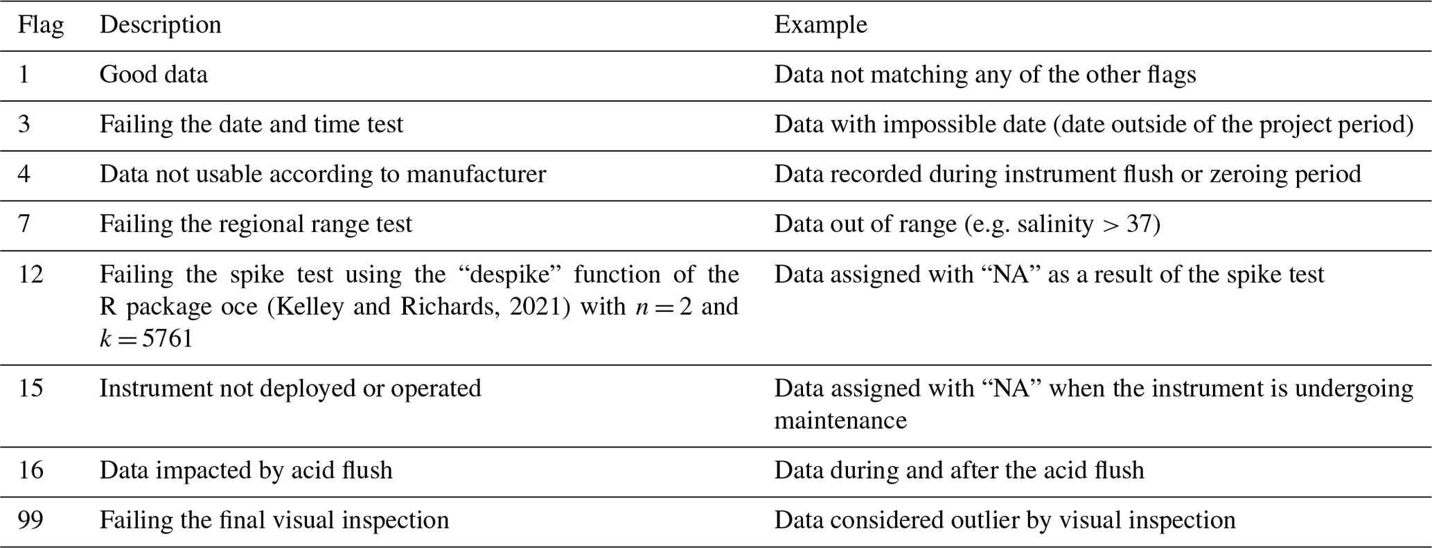
2.3 Partial pressure of CO2
The measuring range of the HydroC CO2 FT sensor (Contros Kongsberg Maritime) is 200–1000 µatm, resolution is < 1 µatm and accuracy is ± 1 % reading. The sensor was positioned first in the loop of sensors of the FerryBox in order to avoid alteration of pCO2 through exposure to air. Two sensors were swapped every year; while one was monitoring pCO2, the other one was factory calibrated. pCO2 was measured continuously, and data were logged every minute. Calibration of the unit was performed by the supplier. It comprised a post-deployment calibration (to assess the drift); a general maintenance, including a change of membrane; and a pre-deployment calibration. This two-step calibration was used to correct the pCO2 data as described by the supplier. Data collected after 1 March 2020 were not used, because the Covid-19 pandemic prevented maintenance and the set-up of a freshly calibrated sensor. As a result, algae became increasingly abundant, pulling pCO2 down and further away from values calculated from CT and AT. pCO2 was expressed at in situ temperature using the pCO2insi function of the R package seacarb v3.3.2 (Gattuso et al., 2023b).
2.4 pH
Two SeaFET ocean pH sensors (Sea-Bird Scientific) were swapped on 17 April 2018 and 2 September 2019. While one was monitoring pH and temperature on the profiler, the other one was factory calibrated. pH (volts) was measured continuously, and data were logged every minute. Calibration was performed as described by Bresnahan et al. (2014) using the functions sf_calib and sf_calc of the R package seacarb v3.3.2 (Gattuso et al., 2023b). Voltage values measured below 8 m in each of the three deployment periods were converted to pH on the total scale (pHT). Field calibration samples for pH were collected using a Niskin bottle close to SeaFET within 15 min of measurement. pH was measured spectrophotometrically (Dickson et al., 2007) with purified m-cresol purple (purchased from Robert H. Byrne's laboratory, University of South Florida). A TRIS standard was measured six times. The deviation between the theoretical pH and pH measured ranged between −0.0033 and +0.0012 pH units (mean = −0.0015). The “pHinsi” function of the R package seacarb v3.3.2 (Gattuso et al., 2023b) was used to express pH at temperatures other than the measurement temperature from pH, salinity and total alkalinity. The dissociation constants used are discussed below.
2.5 Data flow and quality assurance
Data collected at 1 min frequency were assigned with quality flags following a series of quality tests (Table 2). Data with flags other than 1 (good data) were eliminated, and outliers were removed using the despike function of the R package oce (Kelley and Richards, 2021) prior to calculating hourly averages.
2.6 Calculation of derived parameters of the carbonate system
The “carb” function of the R package seacarb v3.3.2 (Gattuso et al., 2023b) was used to calculate all parameters of the carbonate system from pairs of measured variables (e.g. CT and AT, pCO2 and AT, or pH and CT), salinity, temperature and hydrostatic pressure. Total boron concentration was calculated from salinity (Lee et al., 2010). The following constants were used: Kf from Perez and Fraga (1987) and Ks from Dickson (1990). The choice of the stoichiometric dissociation constants and is not obvious in polar oceans (Sulpis et al., 2020). Several sets of formulations were tested: Lueker et al. (2000), Millero et al. (2002), Papadimitriou et al. (2018) and Sulpis et al. (2020). Nutrient data (phosphate and silicate) were taken into consideration whenever available (van de Poll, unpublished data, 2021).
All parameters are reported at in situ temperature unless indicated otherwise. The average uncertainties of the derived carbonate parameters were calculated according to the Gaussian method (Dickson and Riley, 1978) implemented in the “errors” function of the R package seacarb v3.3.2 (Orr et al., 2018; Gattuso et al., 2023b). The uncertainties when using the AT–CT pair are ± 2.7 × 10⁻¹⁰ mol H+ (about 0.015 units pHT), ± 15 µatm pCO2, and ± 0.1 units for the aragonite and calcite saturation states. The maximum additional uncertainty associated with the unavailability of nutrient concentrations (P and Si) as input parameters is comparatively negligible (up to 0.0019 pH units, 1.5 µatm pCO2 and 0.008 Ωa units).
2.7 Air–sea CO2 flux
The instantaneous air–sea CO2 fluxes were calculated as described by De Carlo et al. (2013) from measured pCO2; atmospheric CO2 measured at the Zeppelin station, also located at Ny-Ålesund (data downloaded on 19 August 2020 from https://gaw.kishou.go.jp/search/file/0054-6001-1001-01-01-9999 (last access: 19 August 2020); and the wind speed measured by the Alfred Wegener Institute (AWI) at a height of 10 m (Maturilli, 2020). Two parameterisations between wind speed and the gas transfer velocity k(600) were used (Ho et al., 2006; Dobashi and Ho, 2023).
The following sections describe the dataset that is available at PANGAEA (https://doi.org/10.1594/PANGAEA.957028) and provide first analyses to demonstrate its usefulness.
3.1 Data availability
It is often mentioned that there are fewer observations in the Arctic Ocean than elsewhere, but this is not the case for carbonate variables. We looked at pCO2 records in the v2022 version of the SOCAT database (Bakker et al., 2016, 2022) and the dissolved inorganic carbon (CT) records of the GLODAP v2.2022 database (Lauvset et al., 2022). About 12.4 % of the SOCAT pCO2 records and 11.1 % of the GLODAP CT records are from the Arctic Ocean as defined by the International Hydrographic Organization (1953), which is only about 4.3 % of the global ocean surface area. Coastal (bottom depth < 200 m) data are relatively well represented in both products (24.3 % and 11.1 % of the SOCAT and GLODAP total Arctic data, respectively). The monthly distribution is, however, very uneven with 71.2 % of the SOCAT pCO2 data and 71 % of the GLODAP CT data collected in 4 months of the year (June to September). Furthermore, few to very few data are available for December to March, including in coastal regions. To our knowledge, there is until today no high-frequency, multi-year time-series data.
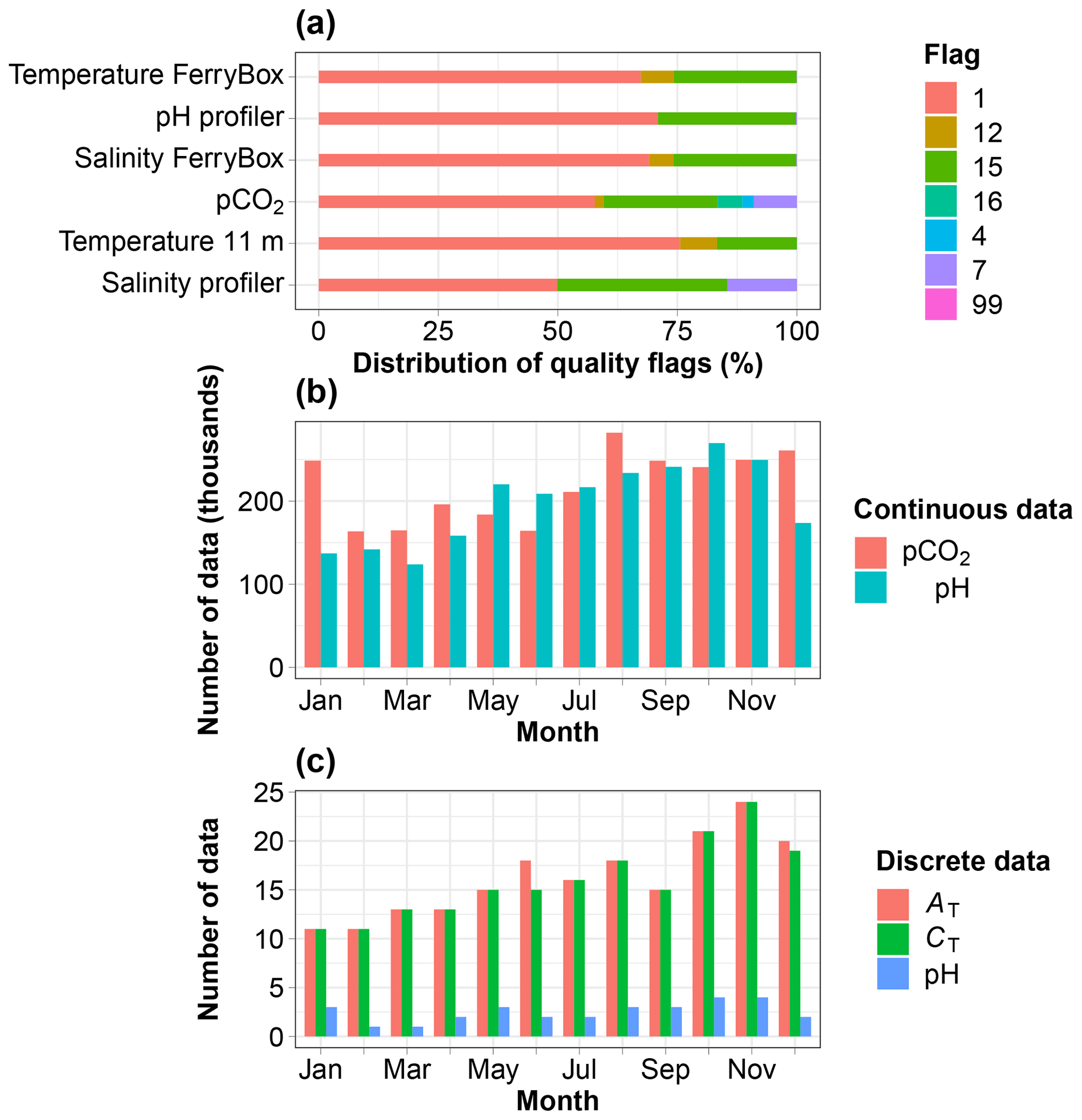
Figure 2(a) Distribution of the quality flags assigned to data collected every minute over the period July 2015 to December 2020, except for the pH profiler sensor (SeaFET), which was set up in August 2017. (b) Monthly distribution of pCO2 and pH data. (c) Monthly distribution of discrete measurements of AT, CT and spectrophotometric pH. Flags are defined in Table 2.
The extreme environmental conditions prevailing at the study site incurred incidents such as interrupted supply of seawater to the FerryBox due to frozen pipes or damage resulting from icebergs pounding on the field instruments. Resolutions to these incidents sometimes took weeks to months due to waiting for warmer temperatures to make deicing possible or due to delays bringing technical staff, including divers, to repair damage. The study site was not accessible for extended periods of time during the Covid-19 pandemic, preventing discrete sampling and resulting in data gaps. The lack of sensor maintenance sometimes generated data of poor quality, which were eliminated, also generating gaps. Nevertheless, data were usable 50 % to 76 % of the time during the period of measurement (Fig. 2a). Continuous pCO2 and pH data are available throughout a composite year and well distributed across months, including in winter months (Fig. 2b). The total numbers of discrete data available for AT, CT and spectrophotometric pH are 195, 191 and 30. They are also well distributed across months (Fig. 2c).
3.2 Impact of the formulations of and
Chen et al. (2015) found that the constants of Mehrbach et al. (1973) and Lueker et al. (2000) yield the best internal consistency in Arctic waters over the temperature range of −1.5 ≤ T ≤ 10.5 ∘C and salinity range of 25.8 ≤ S ≤ 33.1. They recommended the use of these constants. Sulpis et al. (2020) have shown that current estimates of and are inconsistent with measured CO2 system parameters in cold oceanic region. The formulations of Lueker et al. (2000, denoted L00), which are recommended by the community (Jiang et al., 2022), were derived in laboratory conditions with no temperature value below 2 ∘C. These formulations overestimate the stoichiometric dissociation constants at temperatures below about 8 ∘C (Sulpis et al., 2020). There are several alternative formulations. Those of Millero et al. (2002, denoted M02) and (Sulpis et al., 2020, denoted S20) are based on large (> 900) field datasets that include cold-temperature values. The formulations of Papadimitriou et al. (2018, denoted P18), obtained in the laboratory, also cover cold temperatures.
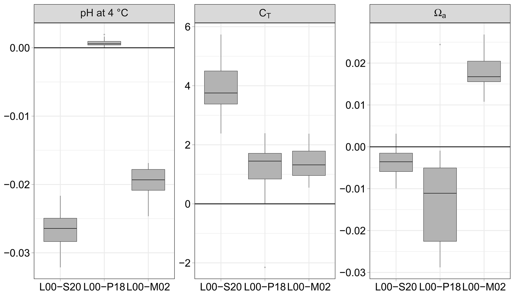
Figure 3pH normalised at 4 ∘C, dissolved inorganic carbon (CT), and saturation state of aragonite Ωa calculated from pCO2 and AT (115 data pairs); differences between the formulations for K1 and K2 of Lueker et al. (2000, L00) and those of Sulpis et al. (2020, S20), Papadimitriou et al. (2018, P18) and Millero et al. (2002, M02). Unit symbols for CT are µmol kg−1.
3.2.1 Using the pair pCO2–AT
For the pair pCO2–AT (115 data pairs), it is the formulation of P18 which provides estimates of pH and CT closest to those obtained with L00 (Fig. 3). The absolute median difference between L00 and P18 is significantly smaller than the uncertainty estimated by error propagation for pH (0.001 vs. 0.004 units) and CT (1.7 vs. 3.6 µmol kg−1). The formulation of M02 performs well for CT (1.5 vs. 3.6 µmol kg−1) but less well for pH (0.019 vs. 0.004 units). The absolute median difference between L00 and S20 is similar to the uncertainty estimated by error propagation for CT (3.7 vs. 3.6 µmol kg−1) but is more than 6 times larger for pH (0.026 vs. 0.004 units). For all formulations, the uncertainty for the saturation state for aragonite is negligible and smaller than that estimated with the propagation of errors.
3.2.2 Using the pair AT–CT
The discrete values of AT, CT, salinity and temperature in the FerryBox were used to calculate pH using the same formulations for and as above (Fig. 3). Overall, the absolute median difference between the formulation of L00, on the one hand, and S20, P18, and M02, on the other hand, is lowest with P18. The absolute median difference L00 minus P18 is small compared to the overall uncertainty estimated by error propagation: 0.004 vs. 0.013 pH units and 3.1 vs. 10.9 µatm pCO2.
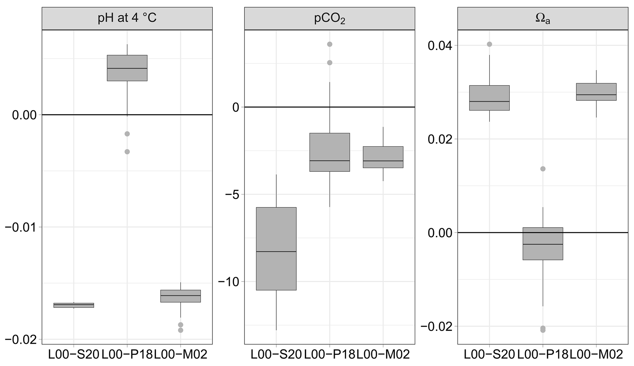
Figure 4pH normalised at 4 ∘C, partial pressure of CO2, and saturation state of aragonite Ωa calculated from AT and CT (115 data pairs); differences between the formulations for K1 and K2 of Lueker et al. (2000, L00) and those of Sulpis et al. (2020, S20), Papadimitriou et al. (2018, P18) and Millero et al. (2002, M02). Units symbols for pCO2 are µatm.
Table 3Difference between spectrophotometric pH and pH calculated with pCO2 and AT using different formulations for and . Q1 and Q3 are the first and third quartiles.
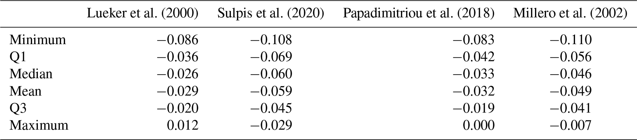
3.2.3 Measured pH vs. pH calculated from pCO2 and AT
Here we compare pH measured spectrophotometrically with pH calculated from pCO2 and AT using various formulations of and (Table 3). All pH values were normalised to a temperature of 4 ∘C. The absolute differences are up to 0.11 pH units. In general, all formulations overestimate spectrophotometric pH. pH calculated using the formulation of Lueker et al. (2000) is closer to measured pH, with a mean difference of −0.029 pH units. This difference is almost 9 times larger than the uncertainty for pH calculated from pCO2 and AT estimated by error propagation (0.004 units). The next closest formulation is the one by Papadimitriou et al. (2018).
Lueker et al. (2000)Sulpis et al. (2020)Papadimitriou et al. (2018)Millero et al. (2002)Table 4Difference between spectrophotometric pH and pH calculated with AT and CT using different formulations for and . Q1 and Q3 are the first and third quartiles.
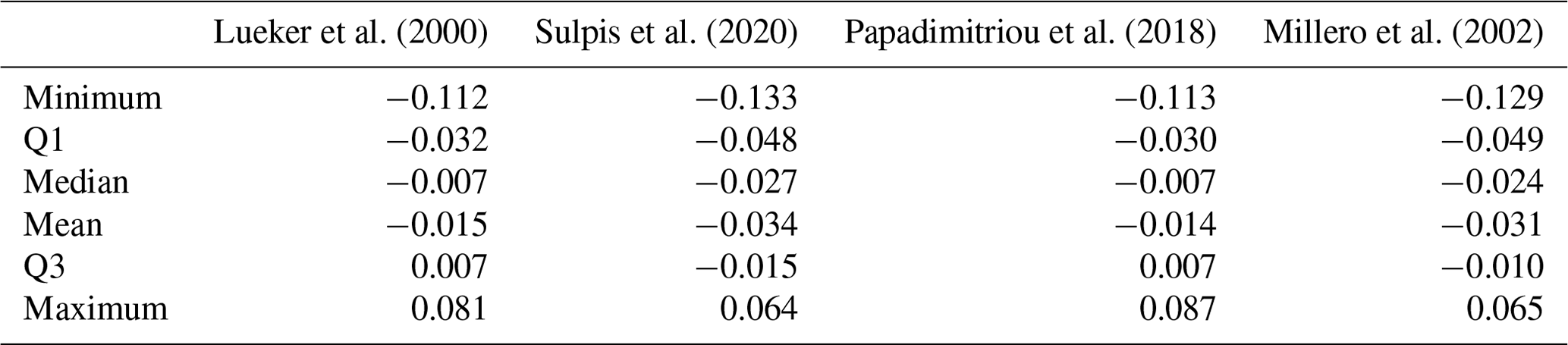
3.2.4 Measured pH vs. pH calculated from AT and CT
Here we compare pH measured spectrophotometrically with pH calculated from discrete measurements of CT and AT using various formulations of and (Table 4). All pH values were normalised to a temperature of 4 ∘C. The absolute differences can be as high as 0.133 pH units. In general, all formulations overestimate spectrophotometric pH. pH calculated using the formulations of Lueker et al. (2000) and Papadimitriou et al. (2018) are closer to measured pH, with absolute median differences of −0.007 pH units. This difference is much smaller than the uncertainty for pH calculated from AT and CT according to seacarb (0.017). The mean differences found with the other formulations are slightly lower than the uncertainty for pH calculated from AT and CT according to seacarb.
In conclusion, the formulations of Lueker et al. (2000) and Papadimitriou et al. (2018) have similar performances with our dataset and generally perform better than those of Millero et al. (2002) and Sulpis et al. (2020). The formulation of Papadimitriou et al. (2018) is seldom used, and the de facto standard has become the formulations of Lueker et al. (2000), which we have used in the present study.
3.3 Impact of nutrient concentrations
Phosphate (PO4) and silicate (Si) contribute to total alkalinity. Changes in their concentration can significantly affect calculations of the carbonate chemistry. The impact on our calculations was checked with a time series of nutrients comprising 90 phosphate and 133 silicate data kindly provided by van de Poll (unpublished data, 2021). At the study site, the concentrations of PO4 and Si vary by a factor of 10 along a composite year. They range between 0.07 and 0.69 µmol kg−1 for PO4 and between 0.42 and 4.7 µmol kg−1 for Si. In our dataset, disregarding the nutrient concentrations does not generate large differences in the derived parameters. Using the pCO2–AT pair of variables, the absolute differences in pH, CT, and Ωa are 0.0001 unit, 0.7 µmol kg−1, and 0.001, respectively. With the CT–AT pair, the absolute differences in pH, pCO2, and Ωa are 0.002 units, < 1.5 µatm, and < 0.01, respectively.
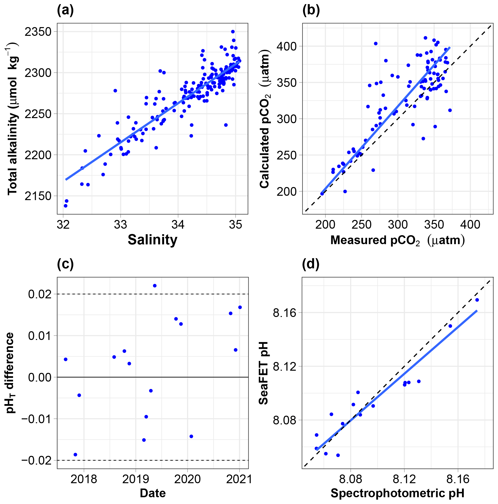
Figure 5(a) Relationship between discrete total alkalinity and salinity; the regression line is estimated using ordinary least square regression. (b) pCO2 calculated from AT and CT vs. pCO2 measured using the Contros sensor. All data are normalised at in situ temperature. The dotted black line is the 1:1 line, while the solid blue line is calculated using a major-axis regression. (c) Offset (total scale) between spectrophotometric measurements of pH and the calibrated SeaFET pH time series. (d) SeaFET pH vs. spectrophotometric pH. All data are on the total scale and normalised at in situ temperature. The dotted black line is the 1:1 line, while the solid blue line is calculated using a major-axis regression.
3.4 Relationship between total alkalinity and salinity
The relationship between the total alkalinity (AT) and salinity (S) is good (Fig. 5a). The equation of the ordinary least square linear regression is (where r2=0.81, N=181). The root mean square error (RMSE) is 16.8 µmol kg−1. Hunt et al. (2021) reported significant seasonal shifts in linear AT vs. S relationships on the east coast of the USA, demonstrating potential problems with any single linear model for the retrieval of AT from salinity. There is no obvious seasonal shift in our dataset. Splitting the data and regressing separately with salinity values below and above 34.5, as done by Nondal et al. (2009) for Nordic open-ocean waters, does not prove useful (data not shown). It degrades r2 (0.74 and 0.3 vs. 0.81) and degrades or marginally improves the RMSE (19 and 13.6 vs. 16.8 µmol kg−1). The relationship above was therefore used to estimate AT from salinity.
3.5 Consistency of measured vs. calculated pCO2
The relationship between the measured and calculated pCO2 (blue line) is relatively poor (Fig. 5b). The slope is 1.12, and its 95 % confidence interval includes 1. The equation of the major-axis regression is the following: calculated pCO2 (µatm) = −23.5 + 1.14 × measured pCO2 (where r2=0.66, N=95).
3.6 Calibration of SeaFET pH sensors and consistency of measured vs. calculated pH
The offset between the spectrophotometric reference samples and the calibrated SeaFET pH time series must be between −0.2 and 0.2 pH units (McLaughlin et al., 2017). The mean offset was ± 0.0026 units, with only one data point outside the recommended range, indicating a high-quality pH dataset (Fig. 5c).
The relationship between spectrophotometric pH and SeaFET pH (blue line) is relatively good (Fig. 5d). The slope is 0.869, and its 95 % confidence interval includes 1. The equation of the major-axis regression is the following: SeaFET pH = 1.06 + 0.869 × spectrophotometric pH (where r2=0.89, N=16).
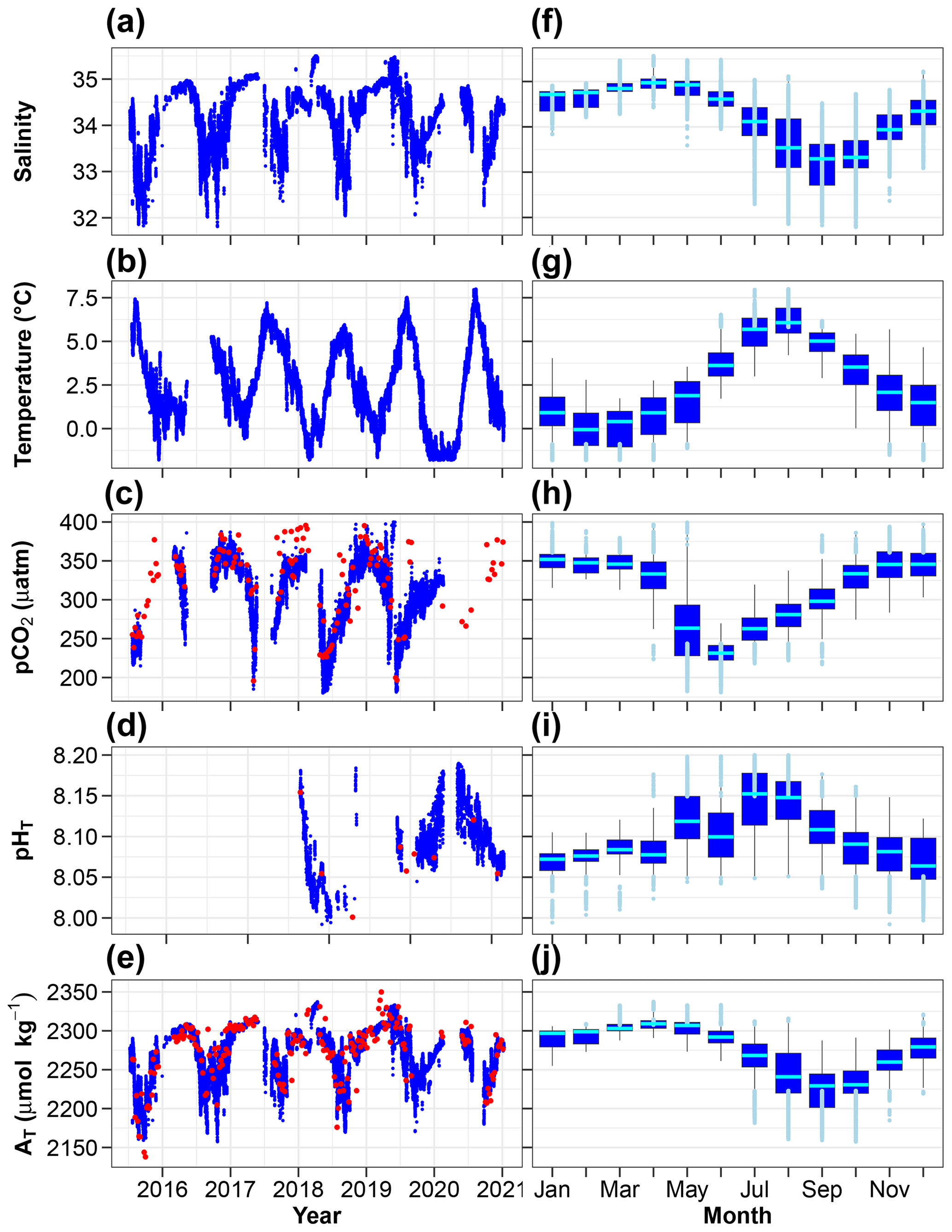
Figure 6Time series (a–e) and monthly distributions (f–j) of key environmental parameters (hourly means). (c) pCO2 measured (red) and calculated using AT and CT (blue). (d) pHT measured (red) and calculated using AT and CT (blue). (e) AT measured by potentiometric titration (red) and calculated from the AT–salinity relationship (blue). In panels (f–j), the cyan lines indicate the medians, boxes show the first and third quartiles as well as the interquartile range, and whiskers extend to the 5th–95th percentiles. The light blue circles highlight values above the 90th percentile and below the 10th percentile.
3.7 Time series and monthly distribution of key parameters
The changes in salinity, temperature, partial pressure of CO2, pH and total alkalinity are shown in Fig. 6a–e and with monthly box plots in Fig. 6f–j. Salinity below 8 m is highest in the spring and lowest in autumn with monthly median values of 35 and 33.3, respectively. Positive salinity extremes (values > 90th percentile) mostly occur in March–June, presumably due to intrusion of seawater from the open sea. Negative salinity extremes (values < 10th percentile) are mostly observed in the summer (defined here as 3 months from June to August) and early autumn, periods during which melting sea ice, calving glaciers and numerous streams release freshwater into the coastal zone. Temperature at 11 m is lowest in February and highest in August with monthly median values of −0.1 and 6.1 ∘C. Total alkalinity exhibits relatively large changes with lower values in the summer and early autumn. Similar and even larger declines have been reported in Spitsbergen fjords (e.g. Koziorowska-Makuch et al., 2023). They are the result of freshwater input which generally has a diluting effect and lowers AT in surface waters.
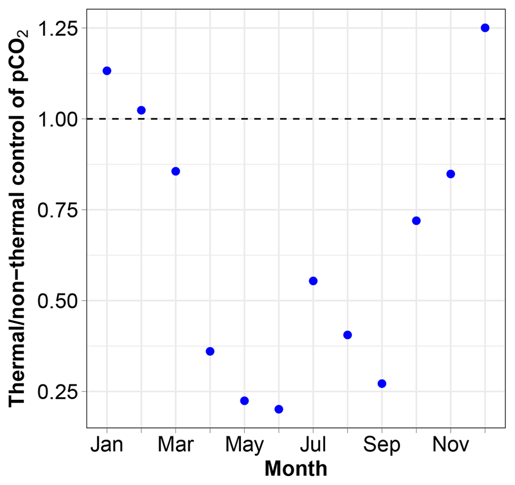
pCO2 at 11 m is almost always lower than 400 µatm with low values during and following the spring phytoplankton bloom and high values in winter. The relative importance of thermal and non-thermal (physical and biological) processes in controlling pCO2 was investigated as described by Takahashi et al. (2002). The thermal/non-thermal ratio is lower than 1 for 9 months of a composite year, indicating that non-thermal drivers exert a greater control than temperature (Fig. 7). The ratio is above 1; hence, thermal control is predominant only in the 3 winter months of December, January and February.
3.8 Depth distribution
There is no depth profile of the variables in the usual sense as the REMOS profiler made stops for 24 h at specific depths to assess the biota in the water column (Fischer et al., 2017). However, the depth distributions of the median monthly salinity, temperature and density provide useful information (Fig. 8). Salinity in the bottom layer (8 to 12 m) is up to 0.9 units higher than in the surface layer (0 to 4 m) in summer, 0.6 units lower in December and relatively similar in both layers at other times. Temperature is lower by up to 2 ∘C in the deep layer than in the surface layer from January to October and higher by up to 0.3 ∘C during November and December. Seawater density is always higher in the bottom layer than in the surface layer (up to 1.2 kg m−3 in July). The 12 m high water column is therefore generally stratified. This is a well-known feature, particularly in the Arctic due to low-salinity surface waters (Dong et al., 2021; Miller et al., 2019).
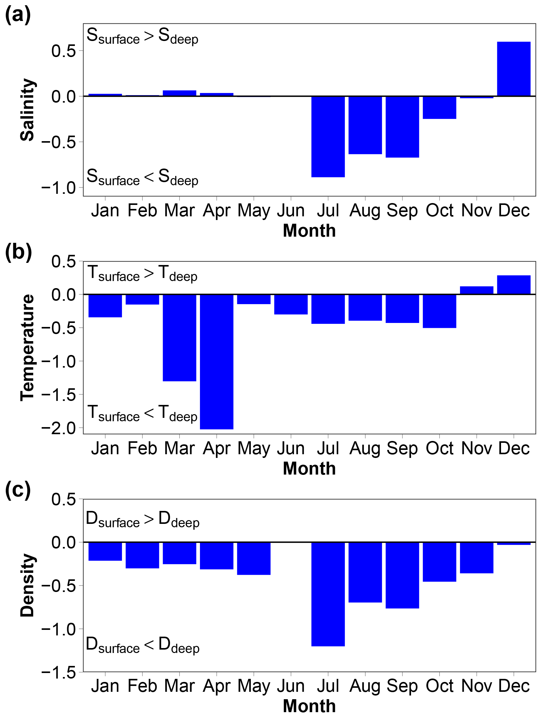
Figure 8Vertical gradients calculated using the median monthly values of salinity (a), temperature (b) and density (c). “Surface” is 0 to 4 m, and “deep” is 8 to 12 m.
3.9 Air–sea CO2 fluxes
pCO2 of seawater pumped at 11 m depth was measured in the FerryBox. This is not the best arrangement to estimate air–sea CO2 fluxes, considering the fact that the water column was sometimes stratified as shown by vertical gradients of salinity, temperature and density (Fig. 8). This is known to have consequences for the air–sea CO2 flux. pCO2 is generally higher in the bottom layer than in the surface layer (note that no data are available in May, June or July).
To estimate air–sea CO2 fluxes, pCO2 can also be calculated using water-column variables measured or estimated from sensors attached to the REMOS device: SeaFET pH, temperature, salinity and salinity-derived total alkalinity. At in situ temperature, the vertical gradient is within ± 4 µatm, except in April when it is more than 40 µatm (Fig. 9a). Normalising pCO2 at 4 ∘C (Fig. 9b) reduces the April difference from −45 to −22.6 µatm, indicating that the vertical gradient is partly driven by temperature.
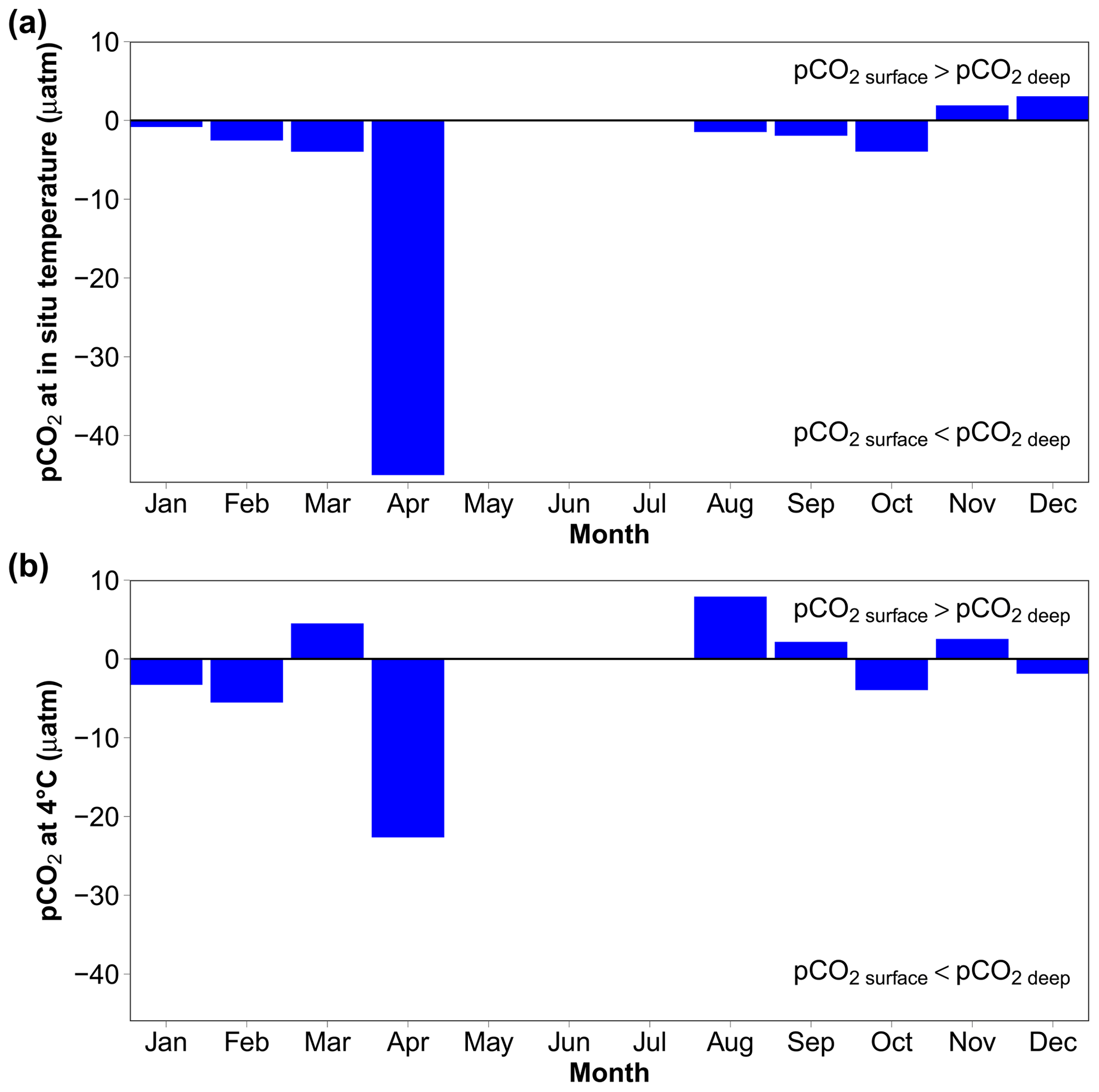
Figure 9Vertical gradients estimated using the median monthly values of pCO2 at in situ hydrostatic pressure, calculated from AT (using the AT vs. S relationship) and SeaFET pHT using the R package seacarb (Gattuso et al., 2023b). (a) CO2 at in situ temperature; (b) pCO2 normalised at 4 ∘C. “Surface” is 0 to 4 m, while “deep” is 8 to 12 m. Data are missing in May to July, because no surface pH data are available during this period.
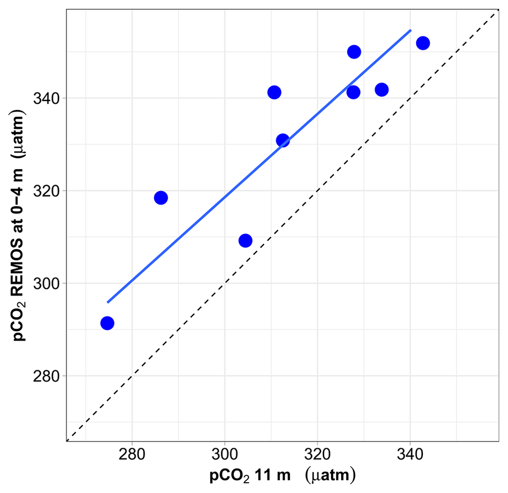
Figure 10Relationship between surface pCO2 (0–4 m) (estimated from pH and salinity-derived AT) and pCO2 at 11 m. Both values are expressed at in situ temperature. The mean and median difference between the two pCO2 values are about 17 µatm. The major-axis regression line is shown in blue, whereas the 1:1 relationship is depicted by a dotted black line.
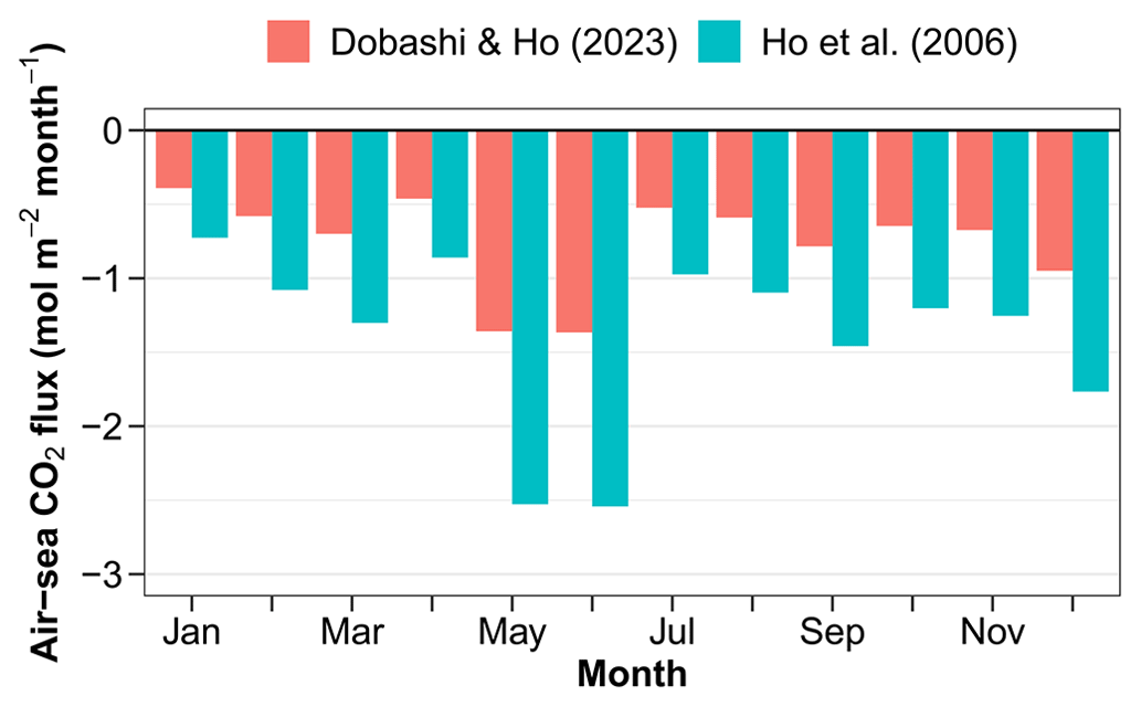
Figure 11Air–sea CO2 fluxes estimated using corrected pCO2 values and the parameterisations of the gas exchange coefficient by wind speed of Ho et al. (2006) and Dobashi and Ho (2023).
For the 9 months when data are available, monthly median pCO2 data normalised at in situ temperature at 11 m vs. 0–4 m are well correlated (r2=0.81), but pCO2 is higher at the surface than at 11 m, with a median difference of 17 µatm (Fig. 10).
The air–sea CO2 flux estimated from pCO2 at 11 m is negative, indicating a CO2 influx from the atmosphere every month of a composite year (Fig. 11). The gas exchange coefficient k is notoriously difficult to measure. It is often parameterised by wind speed, which is known to work well in deep waters offshore (Ho et al., 2006). In shallow areas, parameters other than wind speed become important. Dobashi and Ho (2023) proposed a formulation which might work better in wind-fetch-limited environments. Here we are bracketing the air–sea CO2 flux using these two parameterisations. The annual air–sea flux ranges from −10.2 to −20.2 with the formulations of Dobashi and Ho (2023) and Ho et al. (2006), respectively. Correcting for the fact, discussed above, that surface pCO2 is higher than pCO2 at 11 m leads to fluxes of −16.8 and −9 with the two parameterisations.
These values are in good agreement with the literature. The Arctic Ocean stands out as the region with the strongest CO2 uptake per unit area during the period 1985–2019, with −8.6 ± 0.4 for the open sea and −5.6 ± 0.4 for the continental shelf margins (Chau et al., 2022). Air–sea CO2 flux range from −4 to −86 (Bates and Mathis, 2009; Bates et al., 2011; Rysgaard et al., 2012). For example, the surface waters of the entire Godthåbsfjord (west Greenland) and adjacent continental shelf are undersaturated in CO2 throughout the year (Meire et al., 2015). The average annual CO2 uptake within the fjord is estimated to be 5.42 , indicating that the fjord system is a strong sink for CO2.
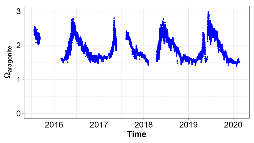
Figure 12Time series of the aragonite saturation state calculated using pCO2 and salinity-derived total alkalinity as input parameters.
3.10 Saturation state of CaCO3
The saturation state of CaCO3 is subject to large interannual changes (Fig. 12). Ωa never becomes lower than 1. It ranges between 1.4 in winter and 3 in summer.
Data are published in the World Data Center PANGAEA (Gattuso et al., 2023a): https://doi.org/10.1594/PANGAEA.960131.
The tab-separated file “AWIPEV-CO2_v2.tab” comprises the following variables (units in brackets when applicable, short names in parentheses):
-
Continuous variables (hourly means).
-
“DATE/TIME” (Date/Time): date and time at UTC+0
-
Pressure, water [dbar] (Press): hydrostatic pressure (profiler)
-
Salinity (Sal): salinity in situ (profiler)
-
Salinity (Sal): salinity (FerryBox)
-
Temperature, water [∘C] (Temp): temperature in situ (static at 11 m)
-
Temperature, water [∘C] (Temp): temperature in situ (CTD, profiler)
-
Temperature, water [∘C] (Temp): temperature in situ (seaFET, profiler)
-
Temperature, water [∘C] (Temp) temperature in the FerryBox
-
Carbon dioxide, partial pressure [µatm] (pCO2): partial pressure of CO2 at in situ temperature (FerryBox)
-
pH (pH): pH on the total scale in situ at in situ temperature (profiler)
-
-
Discrete variables.
-
Alkalinity, total [µmol kg−1] (AT): total alkalinity in situ (discrete)
-
Carbon, inorganic, dissolved [µmol kg−1] (DIC): dissolved inorganic carbon in situ (discrete)
-
pH (pH): spectrophotometric pH on the total scale in situ at in situ temperature (discrete)
-
Although measurements of the carbonate system have increased significantly in the Arctic Ocean, there is still a lack of high-frequency time series, also in the coastal zone. Autonomous time-series measurements in the Arctic involve a number of challenges related to remoteness and the harsh environment (Fischer et al., 2020). The most serious incidents our study faced were related to system damage from iceberg collisions as well as frozen tubes delivering seawater to the land-based measuring system. The remoteness and harsh environmental conditions made maintenance difficult, especially during the polar winter, and led to a discontinuous dataset. Even though we planned this dataset to become a real long-term dataset, unfortunate non-technical circumstances brought this time series to an end, preventing the assessment of interannual variability. Nevertheless, it is unique due to its high (hourly) frequency, coverage of all seasons, and duration (over 4 years).
The final data product provides information on a series of key questions on the dynamics and carbon cycling in a high-Arctic fjord. Several of them have been discussed above. Our results show that (1) the choice of formulations for calculating the dissociation constants of the carbonic acid remains unsettled, (2) the 12 m high water column is consistently stratified most of the time, (3) the calcium carbonate saturation state is subject to large seasonal changes but never reaches undersaturation and (4) this coastal site is a large CO2 sink.
Longer (2012–2021) datasets are available for salinity and temperature (Fischer and colleagues). They are stored in the open-access repository PANGAEA:
-
2012: https://doi.org/10.1594/PANGAEA.896828 (Fischer et al., 2018a)
-
2013: https://doi.org/10.1594/PANGAEA.896822 (Fischer et al., 2018b)
-
2014: https://doi.org/10.1594/PANGAEA.896821 (Fischer et al., 2018c)
-
2015: https://doi.org/10.1594/PANGAEA.896771 (Fischer et al., 2018d)
-
2016: https://doi.org/10.1594/PANGAEA.896770 (Fischer et al., 2018e)
-
2017: https://doi.org/10.1594/PANGAEA.896170 (Fischer et al., 2018f)
-
2018: https://doi.org/10.1594/PANGAEA.897349 (Fischer et al., 2019)
-
2019: https://doi.org/10.1594/PANGAEA.927607 (Fischer et al., 2021a)
-
2020: https://doi.org/10.1594/PANGAEA.929583 (Fischer et al., 2021b)
-
2021: https://doi.org/10.1594/PANGAEA.950174 (Fischer et al., 2022).
JPG conceived the project. PF led the sensor implementation and underwater sensor maintenance. SA and PF maintained the FerryBox system, the instrumentation and the continuous data transfer. SA and JPG led data processing and analysis. JPG led the analysis and writing with contributions from SA and PF. JPG wrote the draft, and co-authors contributed text and edits.
The contact author has declared that none of the authors has any competing interests.
Publisher's note: Copernicus Publications remains neutral with regard to jurisdictional claims in published maps and institutional affiliations.
Thanks are due to Robert Schlegel (Sorbonne Université) for help with data analyses and upload, Li-Qing Jiang (NOAA) for advice about variable names, David Ho for input on gas exchange coefficients, and Mohammed Khamla for assistance with graphics. We also thank Leif Anderson, Yuanxu Dong and Nicolas Metzl for their constructive reviews which significantly improved the paper. We are extremely grateful to the AWIPEV staff who made the continuous operation of the underwater observatory in such a remote location possible almost flawlessly until 2020. Such gratitude cannot be extended to the staff on duty in 2020. We thank the numerous divers from the AWI Centre for Scientific Diving for their invaluable assistance during the maintenance trips. The AT and CT data used in this study were analysed at the SNAPO-CO2 service facility at LOCEAN laboratory and supported by CNRS-INSU and OSU Ecce-Terra. We are indebted to Willem H. van de Poll, who kindly provided nutrient data. We thank Ove Hermansen, Cathrine Lund Myhre and Stephen Platt at the Norwegian Institute for Air Research (NILU) for their assistance with atmospheric CO2 data from the Zeppelin Observatory, as well as the Integrated Carbon Observing System (ICOS)-Norway, Norwegian Research Council project NFR-207587, and the Norwegian Environment Agency. Atmospheric CO2 data from Zeppelin Observatory are available from EBAS: http://ebas.nilu.no (last access: 14 April 2021).
This work has been supported by the Coastal Observing System for Northern and Arctic Seas (COSYNA), the two Helmholtz large-scale infrastructure projects ACROSS and MOSES, the French Polar Institute (IPEV), and by the European Commission, Horizon 2020 Framework Programme (grant nos. 871153, 951799, 727890 and 869154).
This paper was edited by Dagmar Hainbucher and reviewed by Leif Anderson and Yuanxu Dong.
Anderson, L. G., Ek, J., Ericson, Y., Humborg, C., Semiletov, I., Sundbom, M., and Ulfsbo, A.: Export of calcium carbonate corrosive waters from the East Siberian Sea, Biogeosciences, 14, 1811–1823, https://doi.org/10.5194/bg-14-1811-2017, 2017. a
Bakker, D., Alin, S., Becker, M., Bittig, H., Castaño-Primo, R., Feely, R., Gkritzalis, T., Kadono, K., Kozyr, A., Lauvset, S., Metzl, N., Munro, D., Nakaoka, S.-i., Nojiri, Y., O'Brien, K., Olsen, A., Pfeil, B., Pierrot, D., Steinhoff, T., Sullivan, K., Sutton, A., Sweeney, C., Tilbrook, B., Wada, C., Wanninkhof, R., Willstrand Wranne, A., Akl, J., Apelthun, L., Bates, N., Beatty, C., Burger, E., Cai, W.-J., Cosca, C., Corredor, J., Cronin, M., Cross, J., De Carlo, E., DeGrandpre, M., Emerson, S., Enright, M., Enyo, K., Evans, W., Frangoulis, C., Fransson, A., García-Ibáñez, M., Gehrung, M., Giannoudi, L., Glockzin, M., Hales, B., Howden, S., Hunt, C., Ibánhez, J., Jones, S., Kamb, L., Körtzinger, A., Landa, C., Landschützer, P., Lefèvre, N., Lo Monaco, C., Macovei, V., Maenner Jones, S., Meinig, C., Millero, F., Monacci, N., Mordy, C., Morell, J., Murata, A., Musielewicz, S., Neill, C., Newberger, T., Nomura, D., Ohman, M., Ono, T., Passmore, A., Petersen, W., Petihakis, G., Perivoliotis, L., Plueddemann, A., Rehder, G., Reynaud, T., Rodriguez, C., Ross, A., Rutgersson, A., Sabine, C., Salisbury, J., Schlitzer, R., Send, U., Skjelvan, I., Stamataki, N., Sutherland, S., Sweeney, C., Tadokoro, K., Tanhua, T., Telszewski, M., Trull, T., Vandemark, D., van Ooijen, E., Voynova, Y., Wang, H., Weller, R., Whitehead, C., and Wilson, D.: Surface Ocean CO2 Atlas Database Version 2022 (SOCATv2022) (NCEI Accession 0253659), NOAA National Centers for Environmental Information, https://doi.org/10.25921/1h9f-nb73, 2022. a
Bakker, D. C. E., Pfeil, B., Landa, C. S., Metzl, N., O'Brien, K. M., Olsen, A., Smith, K., Cosca, C., Harasawa, S., Jones, S. D., Nakaoka, S., Nojiri, Y., Schuster, U., Steinhoff, T., Sweeney, C., Takahashi, T., Tilbrook, B., Wada, C., Wanninkhof, R., Alin, S. R., Balestrini, C. F., Barbero, L., Bates, N. R., Bianchi, A. A., Bonou, F., Boutin, J., Bozec, Y., Burger, E. F., Cai, W.-J., Castle, R. D., Chen, L., Chierici, M., Currie, K., Evans, W., Featherstone, C., Feely, R. A., Fransson, A., Goyet, C., Greenwood, N., Gregor, L., Hankin, S., Hardman-Mountford, N. J., Harlay, J., Hauck, J., Hoppema, M., Humphreys, M. P., Hunt, C. W., Huss, B., Ibánhez, J. S. P., Johannessen, T., Keeling, R., Kitidis, V., Körtzinger, A., Kozyr, A., Krasakopoulou, E., Kuwata, A., Landschützer, P., Lauvset, S. K., Lefèvre, N., Lo Monaco, C., Manke, A., Mathis, J. T., Merlivat, L., Millero, F. J., Monteiro, P. M. S., Munro, D. R., Murata, A., Newberger, T., Omar, A. M., Ono, T., Paterson, K., Pearce, D., Pierrot, D., Robbins, L. L., Saito, S., Salisbury, J., Schlitzer, R., Schneider, B., Schweitzer, R., Sieger, R., Skjelvan, I., Sullivan, K. F., Sutherland, S. C., Sutton, A. J., Tadokoro, K., Telszewski, M., Tuma, M., van Heuven, S. M. A. C., Vandemark, D., Ward, B., Watson, A. J., and Xu, S.: A multi-decade record of high-quality fCO2 data in version 3 of the Surface Ocean CO2 Atlas (SOCAT), Earth Syst. Sci. Data, 8, 383–413, https://doi.org/10.5194/essd-8-383-2016, 2016. a
Bates, N., Cai, W.-J., and Mathis, J.: The ocean carbon cycle in the western Arctic ocean: distributions and air-sea fluxes of carbon dioxide, Oceanography, 24, 186–201, 2011. a
Bates, N. R. and Mathis, J. T.: The Arctic Ocean marine carbon cycle: evaluation of air-sea CO2 exchanges, ocean acidification impacts and potential feedbacks, Biogeosciences, 6, 2433–2459, https://doi.org/10.5194/bg-6-2433-2009, 2009. a
Bresnahan, PJ, J., Martz, T., Takeshita, Y., Johnson, K., and LaShomb, M.: Best practices for autonomous measurement of seawater pH with the Honeywell Durafet, Methods in Oceanography, 9, 44–60, 2014. a
Chau, T. T. T., Gehlen, M., and Chevallier, F.: A seamless ensemble-based reconstruction of surface ocean pCO2 and air–sea CO2 fluxes over the global coastal and open oceans, Biogeosciences, 19, 1087–1109, https://doi.org/10.5194/bg-19-1087-2022, 2022. a
Chen, B., Cai, W.-J., and Chen, L.: The marine carbonate system of the Arctic Ocean: Assessment of internal consistency and sampling considerations, summer 2010, Mar. Chem., 176, 174–188, 2015. a
Chierici, M. and Fransson, A.: Calcium carbonate saturation in the surface water of the Arctic Ocean: undersaturation in freshwater influenced shelves, Biogeosciences, 6, 2421–2431, https://doi.org/10.5194/bg-6-2421-2009, 2009. a
Comeau, S., Gattuso, J.-P., Nisumaa, A.-M., and Orr, J.: Impact of aragonite saturation state changes on migratory pteropods, P. R. Soc. Lond. B, 279, 732–738, 2011. a
De Carlo, E., Mousseau, L., Passafiume, O., Drupp, P., and Gattuso, J.-P.: Carbonate chemistry and air–sea CO2 flux in a NW Mediterranean Bay over a four-year period: 2007–2011, Aquat. Geochem., 19, 399–442, 2013. a
Dickson, A. G. and Riley, J. P.: The effect of analytical error on the evaluation of the components of the aquatic carbon-dioxide system, Mar. Chem., 6, 77–85, 1978. a
Dickson, A. G., Sabine, C. L., and Christian, J. R.: Guide to best practices for ocean CO2 measurements, PICES Special Publication, 3, 1–191, 2007. a, b, c, d
Dobashi, R. and Ho, D. T.: Air–sea gas exchange in a seagrass ecosystem – results from a tracer release experiment, Biogeosciences, 20, 1075–1087, https://doi.org/10.5194/bg-20-1075-2023, 2023. a, b, c, d
DOE: Handbook of methods for the analysis of the various parameters of the carbon dioxide system in sea water, Carbon Dioxide Information Analysis Center, Oak Ridge National Laboratory, 1994. a
Dong, Y., Yang, M., Bakker, D. C. E., Liss, P. S., Kitidis, V., Brown, I., Chierici, M., Fransson, A., and Bell, T. G.: Near-surface stratification due to ice melt biases arctic air–sea CO2 flux estimates, Geophys. Res. Lett., 48, e2021GL095266, https://doi.org/10.1029/2021GL095266, 2021. a
Edmond, J. M.: High precision determination of titration alkalinity and total carbon dioxide content of sea water by potentiometric titration, Deep-Sea Res., 17, 737–750, 1970. a
Fischer, P., Schwanitz, M., Loth, R., Posner, U., Brand, M., and Schröder, F.: First year of practical experiences of the new Arctic AWIPEV-COSYNA cabled Underwater Observatory in Kongsfjorden, Spitsbergen, Ocean Sci., 13, 259–272, https://doi.org/10.5194/os-13-259-2017, 2017. a, b, c
Fischer, P., Schwanitz, M., Brand, M., Posner, U., Brix, H., and Baschek, B.: Hydrographical time series data of the littoral zone of Kongsfjorden, Svalbard 2012, Alfred Wegener Institute – Biological Institute Helgoland, PANGAEA, https://doi.org/10.1594/PANGAEA.896828, 2018a. a
Fischer, P., Schwanitz, M., Brand, M., Posner, U., Brix, H., and Baschek, B.: Hydrographical time series data of the littoral zone of Kongsfjorden, Svalbard 2013, Alfred Wegener Institute – Biological Institute Helgoland, PANGAEA, https://doi.org/10.1594/PANGAEA.896822, 2018b. a
Fischer, P., Schwanitz, M., Brand, M., Posner, U., Brix, H., and Baschek, B.: Hydrographical time series data of the littoral zone of Kongsfjorden, Svalbard 2014. Alfred Wegener Institute – Biological Institute Helgoland, PANGAEA, https://doi.org/10.1594/PANGAEA.896821, 2018c. a
Fischer, P., Schwanitz, M., Brand, M., Posner, U., Brix, H., and Baschek, B.: Hydrographical time series data of the littoral zone of Kongsfjorden, Svalbard 2015, Alfred Wegener Institute – Biological Institute Helgoland, PANGAEA, https://doi.org/10.1594/PANGAEA.896771, 2018d. a
Fischer, P., Schwanitz, M., Brand, M., Posner, U., Brix, H., and Baschek, B.: Hydrographical time series data of the littoral zone of Kongsfjorden, Svalbard 2016, Alfred Wegener Institute – Biological Institute Helgoland, PANGAEA, https://doi.org/10.1594/PANGAEA.896770, 2018e. a
Fischer, P., Schwanitz, M., Brand, M., Posner, U., Brix, H., and Baschek, B.: Hydrographical time series data of the littoral zone of Kongsfjorden, Svalbard 2017. Alfred Wegener Institute – Biological Institute Helgoland, PANGAEA, https://doi.org/10.1594/PANGAEA.896170, 2018f. a
Fischer, P., Schwanitz, M., Brand, M., Posner, U., Gattuso, J.-P., Alliouane, S., Brix, H., and Baschek, B.: Hydrographical time series data of the littoral zone of Kongsfjorden, Svalbard 2018, Alfred Wegener Institute – Biological Institute Helgoland, PANGAEA, https://doi.org/10.1594/PANGAEA.897349, 2019. a
Fischer, P., Brix, H., Baschek, B., Kraberg, A., Brand, M., Cisewski, B., Riethmüller, R., Breitbach, G., Möller, K., Gattuso, J.-P., Posner, U., Alliouane, S., Loth, R., Van De Poll, W., and Witbaard, R.: Operating cabled underwater observatories in rough shelf-sea environments: a technological challenge, Front. Mar. Sci., 7, 551, https://doi.org/10.3389/fmars.2020.00551, 2020. a, b
Fischer, P., Posner, U., Gattuso, J.-P., Alliouane, S., Spotowitz, L., Schwanitz, M., Brand, M., Brix, H., and Baschek, B.: Hydrographical time series data of the littoral zone of Kongsfjorden, Svalbard 2019, Alfred Wegener Institute – Biological Institute Helgoland, PANGAEA, https://doi.org/10.1594/PANGAEA.927607, 2021a. a
Fischer, P., Spotowitz, L., Posner, U., Schwanitz, M., Brand, M., Gattuso, J.-P., Alliouane, S., Friedrich, M., Brix, H., and Baschek, B.: Hydrographical time series data of the littoral zone of Kongsfjorden, Svalbard 2020, Alfred Wegener Institute – Biological Institute Helgoland, PANGAEA, https://doi.org/10.1594/PANGAEA.929583, 2021b. a
Fischer, P., Happel, L., Lienkämper, M., Spotowitz, L., Brand, M., and Brix, H.: Hydrographical time series data of the littoral zone of Kongsfjorden, Svalbard 2021, PANGAEA, https://doi.org/10.1594/PANGAEA.950174, 2022. a
Fox-Kemper, B., Hewitt, H., Xiao, C., Aðalgeirsdóttir, G., Drijfhout, S., Edwards, T., Golledge, N., Hemer, M., Kopp, R., Krinner, G., Mix, A., Notz, D., Nowicki, S., Nurhati, I., Ruiz, L., Sallée, J.-B., Slangen, A., and Yu, Y.: Ocean, cryosphere and sea level change, in: Climate Change 2021: The Physical Science Basis. Contribution of Working Group I to the Sixth Assessment Report of the Intergovernmental Panel on Climate Change, edited by: Masson-Delmotte, V., Zhai, P., Pirani, A., Connors, S., Péan, C., Berger, S., Caud, N., Chen, Y., Goldfarb, L., Gomis, M., Huang, M., Leitzell, K., Lonnoy, E., Matthews, J., Maycock, T., Waterfield, T., Yelekçi, O., Yu, R., and Zhou, B., 2021. a
Fransson, A., Chierici, M., Nomura, D., Granskog, M., Kristiansen, S., Martma, T., and Nehrke, G.: Effect of glacial drainage water on the CO2 system and ocean acidification state in an Arctic tidewater-glacier fjord during two contrasting years, J. Geophys. Res., 120, 2413–2429, 2015. a
Gattuso, J.-P., Alliouane, S., and Fischer, P.: High-frequency, year-round time series of the carbonate chemistry in a high-Arctic fjord (Svalbard), PANGAEA [data set], https://doi.org/10.1594/PANGAEA.960131, 2023a. a, b
Gattuso, J.-P., Epitalon, J.-M., Lavigne, H., and Orr, J.: seacarb: seawater carbonate chemistry. R package version 3.3.2, https://CRAN.R-project.org/package=seacarb (last access: 1 July 2023), 2023b. a, b, c, d, e, f
Gerland, S. and Renner, A. H.: Sea-ice mass-balance monitoring in an Arctic fjord, Ann. Glaciol., 46, 435–442, 2007. a
Ho, D. T., Law, C. S., Smith, M. J., Schlosser, P., Harvey, M., and Hill, P.: Measurements of air-sea gas exchange at high wind speeds in the Southern Ocean: Implications for global parameterizations, Geophys. Res. Lett., 33, L16611, https://doi.org/10.1029/2006GL026817, 2006. a, b, c, d
Hunt, C., Salisbury, J., Vandemark, D., Aßmann, S., Fietzek, P., Melrose, C., Wanninkhof, R., and Azetsu-Scott, K.: Variability of USA East Coast surface total alkalinity distributions revealed by automated instrument measurements, Mar. Chem., 232, 103960, https://doi.org/10.1016/j.marchem.2021, 2021. a
International Hydrographic Organization: Limits of oceans and seas, Special Publication, 23, 1–45, 1953. a
IOC, SCOR, and IAPSO: The international thermodynamic equation of seawater–2010: calculation and use of thermodynamic properties, Manuals and Guides, 56, 196, Intergovernmental Oceanographic Commission, 2010. a, b
Jakobsson, M., Grantz, A., Kristoffersen, Y., and Macnab, R.: Bathymetry and physiography of the Arctic Ocean and its constituent seas, in: The organic carbon cycle in the Arctic Ocean, edited by: Stein, R. and Macdonald, R. W., Springer, Berlin, https://doi.org/10.1007/978-3-642-18912-8, 1–6, 2004. a
Jiang, L.-Q., Pierrot, D., Wanninkhof, R., Feely, R. A., Tilbrook, B., Alin, S., Barbero, L., Byrne, R. H., Carter, B. R., Dickson, A. G., Gattuso, J.-P., Greeley, D., Hoppema, M., Humphreys, M. P., Karstensen, J., Lange, N., Lauvset, S. K., Lewis, E. R., Olsen, A., Pérez, F. F., Sabine, C., Sharp, J. D., Tanhua, T., Trull, T. W., Velo, A., Allegra, A. J., Barker, P., Burger, E., Cai, W.-J., Chen, C.-T. A., Cross, J., Garcia, H., Hernandez-Ayon, J. M., Hu, X., Kozyr, A., Langdon, C., Lee, K., Salisbury, J., Wang, Z. A., and Xue, L.: Best practice data standards for discrete chemical oceanographic observations, Front. Mar. Sci., 8, 705638, https://doi.org/10.3389/fmars.2021.705638, 2022. a
Kelley, D. and Richards, C.: oce: analysis of oceanographic data, R package version 1.3-0, https://CRAN.R-project.org/package=oce (last access: 26 April 2023), 2021. a, b
Koziorowska-Makuch, K., Szymczycha, B., Thomas, H., and Kuliński, K.: The marine carbonate system variability in high meltwater season (Spitsbergen Fjords, Svalbard), Prog. Oceanogr., 211, 102977, https://doi.org/10.1016/j.pocean.2023.102977, 2023. a
Kwiatkowski, L., Torres, O., Bopp, L., Aumont, O., Chamberlain, M., Christian, J. R., Dunne, J. P., Gehlen, M., Ilyina, T., John, J. G., Lenton, A., Li, H., Lovenduski, N. S., Orr, J. C., Palmieri, J., Santana-Falcón, Y., Schwinger, J., Séférian, R., Stock, C. A., Tagliabue, A., Takano, Y., Tjiputra, J., Toyama, K., Tsujino, H., Watanabe, M., Yamamoto, A., Yool, A., and Ziehn, T.: Twenty-first century ocean warming, acidification, deoxygenation, and upper-ocean nutrient and primary production decline from CMIP6 model projections, Biogeosciences, 17, 3439–3470, https://doi.org/10.5194/bg-17-3439-2020, 2020. a, b
Lantuit, H., Overduin, P. P., Couture, N., Wetterich, S., Aré, F., Atkinson, D., Brown, J., Cherkashov, G., Drozdov, D., Forbes, D. L., Graves-Gaylord, A., Grigoriev, M., Hubberten, H.-W., Jordan, J., Jorgenson, T., Ødegård, R. S., Ogorodov, S., Pollard, W. H., Rachold, V., Sedenko, S., Solomon, S., Steenhuisen, F., Streletskaya, I., and Vasiliev, A.: The Arctic Coastal Dynamics Database: a new classification scheme and statistics on Arctic permafrost coastlines, Estuar. Coast., 35, 383–400, 2012. a
Lauvset, S. K., Lange, N., Tanhua, T., Bittig, H. C., Olsen, A., Kozyr, A., Alin, S., Álvarez, M., Azetsu-Scott, K., Barbero, L., Becker, S., Brown, P. J., Carter, B. R., da Cunha, L. C., Feely, R. A., Hoppema, M., Humphreys, M. P., Ishii, M., Jeansson, E., Jiang, L.-Q., Jones, S. D., Lo Monaco, C., Murata, A., Müller, J. D., Pérez, F. F., Pfeil, B., Schirnick, C., Steinfeldt, R., Suzuki, T., Tilbrook, B., Ulfsbo, A., Velo, A., Woosley, R. J., and Key, R. M.: GLODAPv2.2022: the latest version of the global interior ocean biogeochemical data product, Earth Syst. Sci. Data, 14, 5543–5572, https://doi.org/10.5194/essd-14-5543-2022, 2022. a
Lee, K., Kim, T.-W., Byrne, R. H., Millero, F. J., Feely, R. A., and Liu, Y.-M.: The universal ratio of boron to chlorinity for the North Pacific and North Atlantic oceans, Geochim. Cosmochim. Ac., 74, 1801–1811, 2010. a
Lueker, T. J., Dickson, A., and Keeling, C. D.: Ocean pCO2 calculated from dissolved inorganic carbon, alkalinity, and equations for K1 and K2: validation based on laboratory measurements of CO2 in gas and seawater at equilibrium, Mar. Chem., 70, 105–119, 2000. a, b, c, d, e, f, g, h, i, j
Maturilli, M.: Continuous meteorological observations at station Ny-Ålesund (2011-08 et seq), PANGAEA, 23–46, https://doi.org/10.1594/PANGAEA.914979, 2020. a
McLaughlin, K., Dickson, A., Weisberg, S., Coale, K., Elrod, V., Hunter, C., Johnson, K., Kram, S., Kudela, R., Martz, T., Negrey, K., Passow, U., Shaughnessy, F., Smith, J., Tadesse, D., Washburn, L., and Weis, K.: An evaluation of ISFET sensors for coastal pH monitoring applications, Regional Studies in Marine Science, 12, 11–18, 2017. a
Mehrbach, C., Culberson, C. H., Hawley, J. E., and Pytkowicz, R. M.: Measurement of the apparent dissociation constants of carbonic acid in seawater at atmospheric pressure, Limnol. Oceanogr., 18, 897–907, 1973. a
Meire, L., Søgaard, D. H., Mortensen, J., Meysman, F. J. R., Soetaert, K., Arendt, K. E., Juul-Pedersen, T., Blicher, M. E., and Rysgaard, S.: Glacial meltwater and primary production are drivers of strong CO2 uptake in fjord and coastal waters adjacent to the Greenland Ice Sheet, Biogeosciences, 12, 2347–2363, https://doi.org/10.5194/bg-12-2347-2015, 2015. a
Menard, H. W. and Smith, S. M.: Hypsometry of ocean basin provinces, J. Geophys. Res., 71, 4305–4325, 1966. a
Miller, L. A., Burgers, T. M., Burt, W. J., Granskog, M. A., and Papakyriakou, T. N.: Air–sea CO2 flux estimates in stratified arctic coastal waters: how wrong can we be, Geophys. Res. Lett., 46, 235–243, 2019. a
Millero, F. J., Pierrot, D., Lee, K., Wanninkhof, R., Feely, R., Sabine, C. L., Key, R. M., and Takahashi, T.: Dissociation constants for carbonic acid determined from field measurements, Deep-Sea Res. Pt. I, 49, 1705–1723, 2002. a, b, c, d, e, f
Nondal, G., Bellerby, R. G. J., Olsen, A., Johannessen, T., and Olafsson, J.: Optimal evaluation of the surface ocean CO2 system in the northern North Atlantic using data from voluntary observing ships, Limnol. Oceanogr. Meth., 7, 109–118, 2009. a
Orr, J., Epitalon, J.-M., Dickson, A., and Gattuso, J.-P.: Routine uncertainty propagation for the marine carbon dioxide system, Mar. Chem., 207, 84–107, 2018. a
O'Neill, B., Oppenheimer, M., Warren, R., Hallegatte, S., Kopp, R., Pörtner, H., Scholes, R., Birkmann, J., Foden, W., Licker, R., Mach, K., Marbaix, P., Mastrandrea, M., Price, J., Takahashi, K., van Ypersele, J.-P., and Yohe, G.: IPCC reasons for concern regarding climate change risks, Nat. Clim. Change, 7, 28–37, 2017. a
Papadimitriou, S., Loucaides, S., Rérolle, V. M., Kennedy, P., Achterberg, E. P., Dickson, A. G., Mowlem, M., and Kennedy, H.: The stoichiometric dissociation constants of carbonic acid in seawater brines from 298 to 267 K, Geochim. Cosmochim. Ac., 220, 55–70, 2018. a, b, c, d, e, f, g, h, i
Pavlova, O., Gerland, S., and Hop, H.: Changes in sea-Ice extent and thickness in Kongsfjorden, Svalbard (2003–2016), in: The ecosystem of Kongsfjorden, Svalbard, edited by: Hop, H. and Wiencke, C., Springer, Cham, https://doi.org/10.1007/978-3-319-46425-1, 105–136, 2019. a
Perez, F. F. and Fraga, F.: Association constant of fluoride and hydrogen ions in seawater, Mar. Chem., 21, 161–168, 1987. a
Rysgaard, S., Mortensen, J., Juul-Pedersen, T., Sørensen, L., Lennert, K., Søgaard, D., Arendt, K., Blicher, M., Sejr, M., and Bendtsen, J.: High air-sea CO2 uptake rates in nearshore and shelf areas of Southern Greenland: Temporal and spatial variability, Mar. Chem., 128–129, 26–33, 2012. a
Shiklomanov, I.: Comprehensive assessment of the freshwater resources of the world: assessment of water resources and water availability in the world, World Meteorological Organization, Geneva, 1998. a
Stein, R. and Macdonald, R. W.: Organic carbon budget: Arctic Ocean vs. glocal ocean, in: The organic carbon cycle in the Arctic Ocean, edited by: Stein, R. and Macdonald, R. W., Springer, Berlin, 315–322, https://doi.org/10.1007/978-3-642-18912-8, 2004. a
Sulpis, O., Lauvset, S. K., and Hagens, M.: Current estimates of and appear inconsistent with measured CO2 system parameters in cold oceanic regions, Ocean Sci., 16, 847–862, https://doi.org/10.5194/os-16-847-2020, 2020. a, b, c, d, e, f, g, h, i
Takahashi, T., Sutherland, S. C., Sweeney, C., Poisson, A., Metzl, N., Tilbrook, B., Bates, N., Wanninkhof, R., Feely, R. A., and Sabine, C.: Global sea–air CO2 flux based on climatological surface ocean pCO2, and seasonal biological and temperature effects, Deep-Sea Res. Pt. II, 49, 1601–1622, 2002. a
Vihtakari, M.: ggOceanMaps: plot data on oceanographic maps using “ggplot2”, R package version 1.3.4, https://CRAN.R-project.org/package=ggOceanMaps (last access: 26 April 2023), 2022. a
Wassmann, P., Duarte, C., Agustí, S., and Sejr, M.: Footprints of climate change in the Arctic marine ecosystem, Glob. Change Biol., 17, 1235–1249, 2010. a
Zhang, Y., Yamamoto-Kawai, M., and Williams, W.: Two decades of ocean acidification in the surface waters of the Beaufort Gyre, Arctic Ocean: effects of sea ice melt and retreat from 1997–2016, Geophys. Res. Lett., 47, e60119, https://doi.org/10.1029/2019GL086421, 2020. a