Wind wave and water level dataset for Hornsund, Svalbard (2013–2021)

Underwater pressure sensors were deployed near-continuously at various locations of the nearshore (8–23 m depth) Hornsund fjord, Svalbard, between July 2013 and February 2021. Raw pressure measurements at 1 Hz were used to derive mean water levels, wave spectra and bulk wave parameters for 1024 s bursts at hourly intervals. The procedure included subtracting atmospheric pressure, depth calculation, fast Fourier transform, correction for the decrease of the wave orbital motion with depth and adding a high-frequency tail. The dataset adds to the sparse in situ measurements of wind waves and water levels in the Arctic, and it can be used, for example, for analysing seasonal wind wave conditions and inter-annual trends and calibrating/validating wave models. The dataset is stored in the PANGAEA repository (https://doi.org/10.1594/PANGAEA.954020; Swirad et al., 2023).

1 Introduction

In situ wave measurements are critical for understanding wave climate, analysing seasonal and inter-annual trends, and calibrating and validating wave transformation models (e.g. Reistad et al., 2011). The spatial distribution of instruments providing wind wave data is irregular and tends to concentrate in mid- and low-latitude coastal areas (e.g. https://www.ndbc.noaa.gov/, 28 November 2022; Semedo et al., 2015). In the Arctic, the network of such instruments is particularly sparse. There is a pertinent lack of continuous wave data in the Svalbard archipelago where communities, industry infrastructure, and research stations are located. Continuous wave observations in the coastal Arctic are needed to better understand how the following contribute to coastal flooding and erosion that can cause infrastructure damage (Forbes, 2011): (i) decreasing sea-ice extent – pan-Arctic annual mean extent decrease of 3.5 %–4.1 % per decade (IPCC, 2019) or 1.5- to 3-fold increase in the length of the sea-ice-free season along pan-Arctic coasts (Barnhart et al., 2014) between 1979 and 2012; (ii) increasing frequency and strength of storms (Francis et al., 2011; Wang et al., 2015; Stopa et al., 2016; Waseda et al., 2018); and, in consequence, (iii) higher waves acting on Arctic coasts for longer time periods.

Our knowledge of the western Svalbard wave climate comes primarily from global spectral models such as NOAA's WaveWatch III (WW3) hindcast (WW3DG, 2019); ECMWF reanalysis projects ERA-40 (1957–2002; Uppala et al., 2005), ERA-Interim (1979–2019; Dee et al., 2011), and ERA5 (1959–present; Hersbach et al., 2020); or NCEP's Climate Forecast System Reanalysis (CFSR; Saha et al., 2014). Arctic Ocean Wave Analysis and Forecast system (Carrasco et al., 2022) is a shorter-duration (since 2017), higher-resolution (3 km) model that provides hourly significant wave height (H_s), peak period (T_p) and peak wave direction (θ_p) using ECMWF's Ocean Wave Model (WAM). The 10 km resolution ERA-40 reanalysis data allowed Semedo et al. (2015) to capture seasonal trends in swell and wind sea and the ≥ 10 cm per decade increase in winter H_s over the northern Atlantic. Stopa et al. (2016) used CFSR and altimetry data to calculate an average H_s of 1.5 m (99th percentile of 5–6 m) for the period 1992–2014 west of Svalbard. Wojtysiak et al. (2018) observed up to 1 m H_s difference between winter (higher) and summer (lower) months using WW3 (2005–2015; at 0.5^∘ resolution) and ERA-Interim (1979–2015; at 1^∘ resolution), and they found a statistically significant trend of increasing frequency (2 storms per decade) and total duration (4 d per decade) of storms for the Greenland Sea off south-western Svalbard for the 1979–2015 period, with the typical annual values of 10–40 storms and 20–80 d, respectively.

The large-scale models are good for understanding the general trends in the Arctic/Svalbard area but provide limited information on local-scale wave parameters in specific fjords and bays (Nederhoff et al., 2022). How the open ocean wave conditions translate into wave conditions in the coastal areas is poorly constrained given complex coastal wind patterns and bottom topography (Semedo et al., 2015). Moreover, the large-scale models oversimplify most aspects of wind wave–sea ice interactions. Most operational models use simple empirical formulae for wave attenuation in sea ice (Barnhart et al., 2014; Zhao et al., 2015; Ardhuin et al., 2016).

Herman et al. (2019) used three nested Simulating WAves Nearshore (SWAN; Booij et al., 1999) models to predict wind wave parameters within bays of Hornsund fjord (∼ 15 m depth), taking eastern Greenland Sea WW3 spectra as boundary conditions. They ran the model for two sea-ice-free 4-month periods (August–November 2015 and 2016), finding a good agreement between the modelled and measured significant wave height (r² > 0.9) and mean absolute wave period (r² = 0.63–0.78). The study added considerable detail to wind wave transformation in the nearshore environment of Hornsund by including fjord bathymetry, which allowed for resolving depth-induced wave breaking and bottom friction on wind conditions. Notably, the study used a subset of the dataset described in this paper to validate the wave spectral model (Herman et al., 2019).

The model of Herman et al. (2019) tested against buoy data performed well for ice-free conditions only. For a bay of the Beaufort Sea, Nederhoff et al. (2022) incorporated sea ice into the SWAN model, which enabled them to reliably describe wave climate in 1979–2019. The need for observational data to validate wave models, especially in periods when the sea ice is present, persists.

We present a 7.5-year (July 2013 to February 2021) wind wave dataset from Hornsund, southern Svalbard (77^∘ N, 15.5^∘ E). Our goal is to increase observational understanding of Arctic wave conditions by providing a dataset that can be further used to (i) analyse the inter- and intra-annual trends in nearshore wind wave conditions, (ii) calibrate and validate wave transformation models, (iii) quantify the role of sea ice in wave attenuation, (iv) create empirical models of wave run-up on high-latitude beaches, and (v) predict future wind wave conditions.

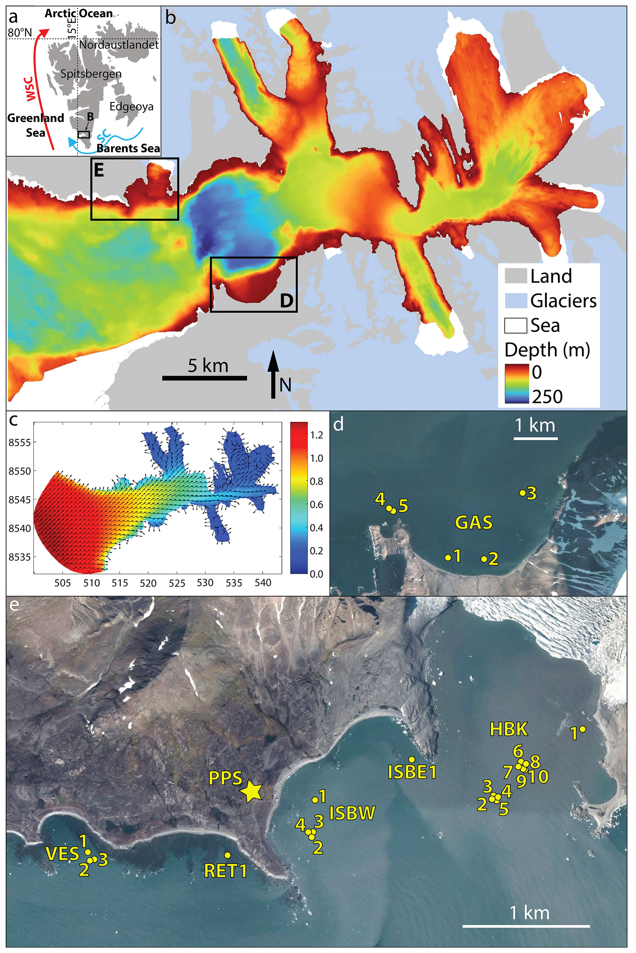
Figure 1 Study area: (a) Svalbard archipelago; WSC = warm West Spitsbergen Current; SC = cold Sørkapp Current; (b) bathymetry of Hornsund fjord (source: Norwegian Hydrographic Service; permit granted to IG PAS); (c) mean significant wave height, H_s (colours, in metres, m) and wind wave direction, θ_p (arrows) from Herman et al. (2019); axis labels refer to Universal Transverse Mercator coordinate system zone 33X (UTM33X) coordinates (in kilometres, km); location of sensor deployments in southern (d) and northern (e) Hornsund. HBK = Hansbukta, ISB = Isbjørnhamna (W = western, E = eastern), RET = Rettkvalbogen, GAS = Gåshamna, VES = Veslebogen, PPS = Polish Polar Station. Background image © Norwegian Polar Institute (permit granted).

2 Study area

Hornsund is an ∼ 30 km long fjord of SW Spitsbergen, Svalbard (Fig. 1a). It has an ∼ 12 km wide and ∼ 100 m deep opening to the Greenland Sea. The average fjord depth is ∼ 100 m with the deeper (200–250 m) central part (Fig. 1b; Herman et al., 2019). The tides are semi-diurnal, and the average tidal range is 0.75 m (Kowalik et al., 2015). The circulation is cyclonic (anticlockwise) with the inflow from SW and outflow to the NW (Jakacki et al., 2017).

In 1979–2018 easterly winds dominated at the Polish Polar Station (12 $\mathrm{m}\mathrm{a}.\mathrm{s}.\mathrm{l}.$; PPS in Fig. 1e) with the mean direction of 124^∘ (annual mean range of 102–140^∘). Mean wind speed at ∼ 20 $\mathrm{m}\mathrm{a}.\mathrm{s}.\mathrm{l}.$ was 5.5 m s⁻¹ (Wawrzyniak and Osuch, 2020).

Wave conditions in Hornsund are usually related to the long oceanic swell or mixed swell/wind sea from S–SW with short wind waves formed locally due to predominantly easterly winds. The mean H_s at the fjord mouth is 1.2–1.3 m, decreasing to 0.5–0.9 m in the central and to < 0.4 m in the inner parts of Hornsund (Fig. 1c). Northern shores of the fjord receive more wave energy than southern shores (Herman et al., 2019).

Hornsund bays (in this study Hansbukta, Isbjørnhamna, Rettkvalbogen, Veslebogen and Gåshamna) have complex shapes and bottom topography with ubiquitous skerries causing strong wave transformation due to refraction and dissipation (Herman et al., 2019).

Sea ice forms locally in the fjord or drifts from the open Greenland Sea. The latter originates east of Svalbard, drifts past the southern tip of Spitsbergen (Sørkapp) and then drifts northwards along the western Spitsbergen coast with cold Sørkapp Current (blue arrow in Fig. 1a). Fast ice (i.e. sea ice attached to the shore) persists during winter months. Muckenhuber et al. (2016) observed a decrease in sea-ice (both drift and fast ice) duration and extent between 2000 and 2014. In summer months glacier ice from calving tide-water glaciers (Błaszczyk et al., 2019) may accumulate in bays. Increased storminess coincident with positive air temperature anomalies and the lack of sea ice, in particular during October–December, may contribute to coastal erosion (Zagórski et al., 2015).

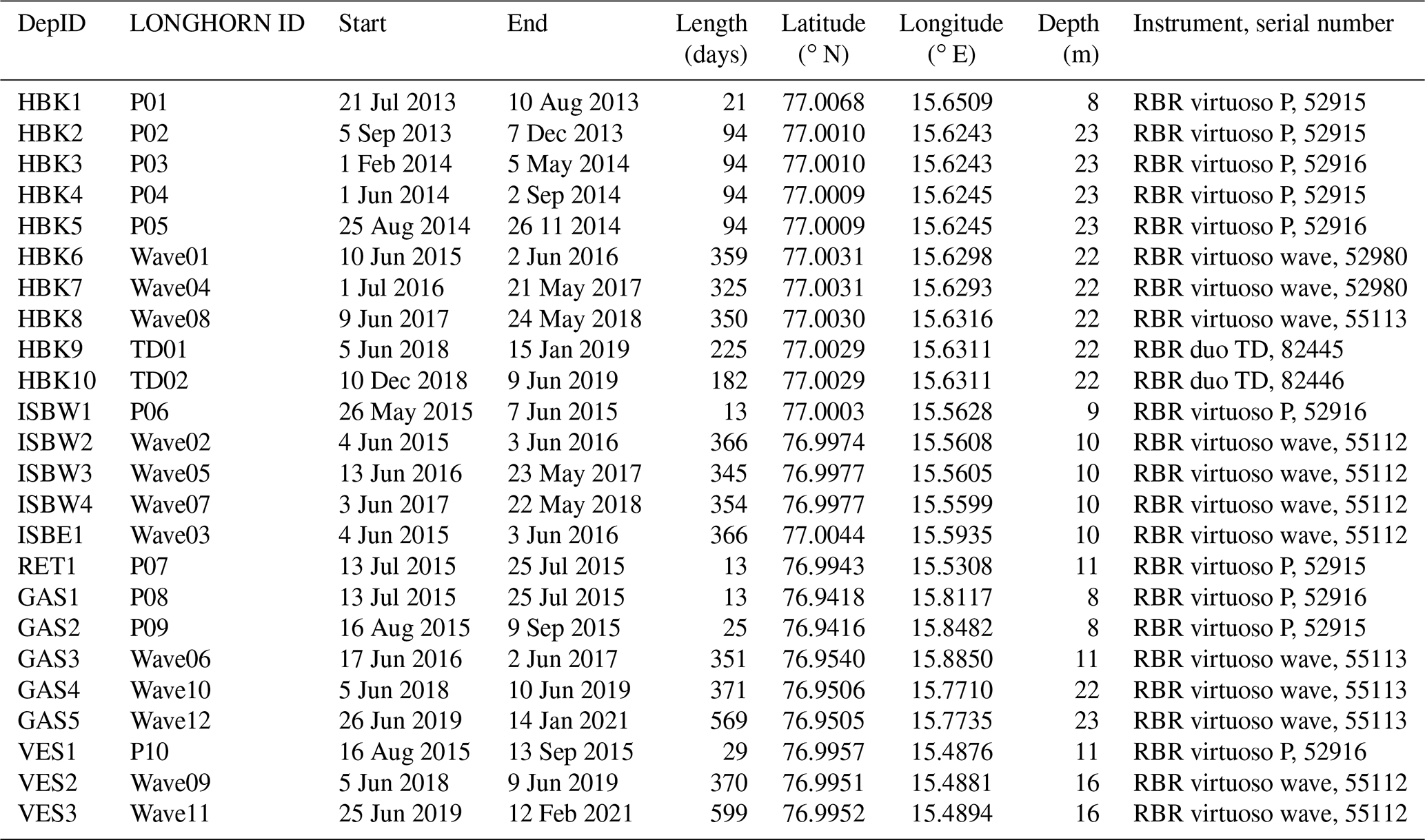
Table 1 Details of the pressure sensor deployments for in situ wave measurements in Hornsund, Svalbard. Deployment ID (DepID) refers to bays: HBK = Hansbukta, ISB = Isbjørnhamna (W = western, E = eastern), RET = Rettkvalbogen, GAS = Gåshamna, VES = Veslebogen. LONGHORN ID refers to the IG PAS oceanographic monitoring (Swirad et al., 2022).

3 Methods

3.1 Input data

Pressure data were collected between 21 July 2013 and 12 February 2021 using RBR virtuoso P (continuous sampling at 4 or 6 Hz interval), RBR duo TD (continuous sampling at 1 Hz interval) and RBR virtuoso wave sensors (1024 s bursts at 30 min interval with 1 Hz sampling interval or at 60 min interval with 2 Hz sampling interval). There were 24 single deployments with a duration of 13–599 d (Table 1; Fig. 2). Initially the deployments were short ( < 100 d) and usually restricted to the fieldwork season (late spring to autumn). Since 2015, however, deployments were typically ∼ 1-year long with instrument recovery and redeployment during summer field campaigns. As a result of the COVID-19 pandemic, it was impossible to recover instruments in summer 2020, and the last two deployments (GAS5 and VES3) were > 550 d long and ended with the battery going dead.

The instruments were anchored to the seabed in various locations in northern (Hansbukta, western and eastern Isbjørnhamna, Rettkvalbogen, Veslebogen) and southern (Gåshamna) Hornsund (Fig. 1d and e). The raw pressure data are part of the LONGHORN oceanographic monitoring of the Institute of Geophysics, Polish Academy of Sciences, (IG PAS) and are provided in Swirad et al. (2022).

For consistency, the raw data were subsampled to 1024 s bursts at 60 min interval (starting at full hours) with 1 Hz sampling interval. The erroneous bursts at the start and end of deployments were removed. The datasets were cropped to full days so that the first measurement occurs at 00:00:00 UTC (hh:mm:ss) and the last one at 23:17:03 (1024 s after 23:00). These 24 deployment files are time series with three columns representing time, burst number and raw pressure (in dbar), and they are available as part of the dataset (Swirad et al., 2023).

3.2 Burst processing

The deployment files were imported into Spyder (Python 3.9) and processed on the burst-by-burst basis, with an algorithm described below (see also Wang et al., 1986; Karimpour and Chen, 2017; Marino et al., 2022, and references therein). Importantly, all steps described below are based on the linear wave theory; alternative data processing methods (e.g. Bonneton et al., 2018) might be applied to the original burst data to capture non-linear effects, but they are not considered here.

Hourly (one per burst) atmospheric pressure P_air (mbar) data at sea level were taken from the Polish Polar Station archive (https://monitoring-hornsund.igf.edu.pl/, last access: 28 March 2022). The water pressure, P_sea (dbar), was calculated by subtracting atmospheric pressure from the raw pressure, P_raw:

$$\begin{array}{}\text{(1)}& P_{\text{sea}}=P_{\text{raw}}-P_{\text{air}}/\mathrm{100}.\end{array}$$

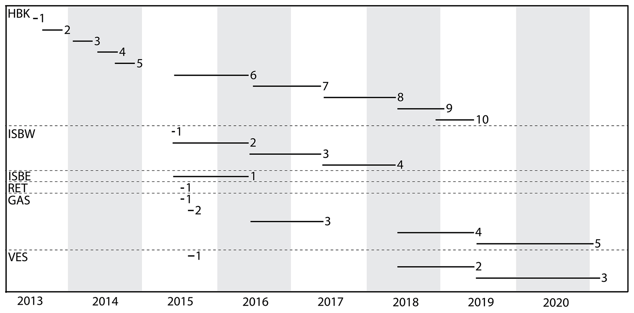
Figure 2 Time span of pressure sensor deployments for in situ wave measurements in Hornsund, Svalbard. HBK = Hansbukta, ISB = Isbjørnhamna (W = western, E = eastern), RET = Rettkvalbogen, GAS = Gåshamna, VES = Veslebogen.

Depth, z (m), was calculated using the UNESCO formula (Fofonoff and Millard, 1983) under assumption of constant water temperature of 0 ^∘ C, salinity of 35 PSU and latitude φ = 77^∘ N:

$$\begin{array}{}\text{(2)}& \begin{array}{rl}z=& \left[\left(\left(\left(-\mathrm{1.82}\times {\mathrm{10}}^{-\mathrm{15}}{P}_{\text{sea}}+\mathrm{2.279}\times {\mathrm{10}}^{-\mathrm{10}}\right)P_{\text{sea}}\right.\right.\right.\\ & \left.\left.\left.-\mathrm{2.2512}\times {\mathrm{10}}^{-\mathrm{5}}\right)P_{\text{sea}}+\mathrm{9.72659}\right)P_{\text{sea}}\right]/g,\end{array}\end{array}$$

where g (m s⁻²) denotes acceleration due to gravity, computed as

$$\begin{array}{}\text{(3)}& \begin{array}{rl}g=& \mathrm{9.780318}[\mathrm{1}+(\mathrm{5.2788}\times {\mathrm{10}}^{-\mathrm{3}}+\mathrm{2.36}\times {\mathrm{10}}^{-\mathrm{5}}x\left)x\right]\\ & +\mathrm{1.092}\times {\mathrm{10}}^{-\mathrm{6}}{P}_{\text{sea}},\end{array}\end{array}$$

and x is given by

$$\begin{array}{}\text{(4)}& x={\sin }^{\mathrm{2}}(\mathit{\phi }/\mathrm{57.29578}).\end{array}$$

The slowly varying component of water depth (due to, for example, tide and storm surge) was removed by subtracting from z a least-square-fitted second-order polynomial trend, z_lf, resulting in time series z_hf (m), related to depth variability associated with wind waves: z_hf = z−z_lf. The energy density spectrum at depth z, E_z(f) (in m² s), was computed by applying fast Fourier transform (FFT; Frigo and Johnson, 2005) to the time series z_hf. As already mentioned, the data length used for FFT input was 1024. The Python fft function with default settings was used to compute the spectra, and no windowing was applied.

Finally, the spectrum at the sea surface, E₀(f), was computed from E_z(f) by applying a correction factor A(f) accounting for the decrease of the wave orbital motion (and thus pressure fluctuations) with depth (compare red and blue spectra in Fig. 3):

$$\begin{array}{}\text{(5)}& E_{\mathrm{0}}\left(f\right)=E_z\left(f\right)/A\left(f\right).\end{array}$$

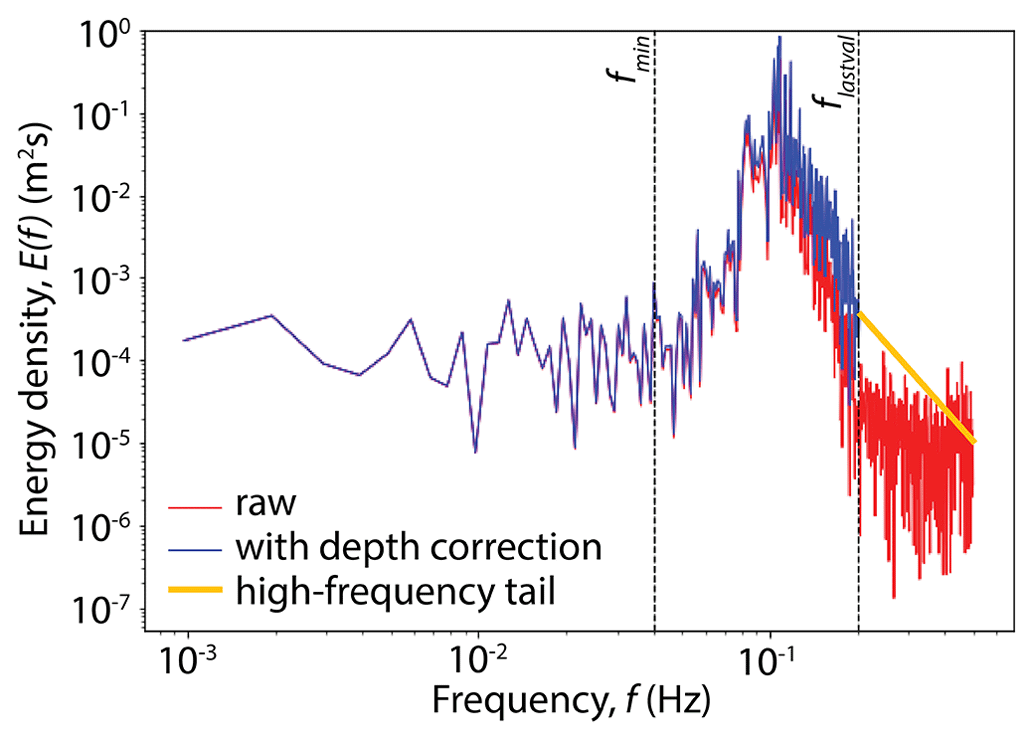
Figure 3 An example of wave energy density spectrum computed with the algorithm described in the text (deployment HBK9 burst no. 1): raw spectrum E_z(f) at the depth of the logger (red), depth-corrected spectrum E₀(f) (blue), and the analytical high-frequency tail (yellow). Frequency f_min = 0.04 Hz is the minimum frequency used to calculate mean wave parameters, and f_lastval is the highest frequency reliably measured. The plot is limited to f = 0.5 Hz, which is the upper limit of the observation data. Wave parameters are calculated in two versions: for f_min < f < f_lastval and for f_min < f < ∞.

To this end, a set K of basic wavenumber values was defined, K = $\mathit{\{}\mathrm{0},\mathrm{0.01},\mathrm{0.02},\mathrm{\dots },\mathrm{1000}\mathit{\}}$ (m⁻¹), and a corresponding set of basic wave frequencies, F, with the following elements:

$$\begin{array}{}\text{(6)}& f_i=\sqrt{g{k}_i\tanh \left(k_{i}h\right)}/\left(\mathrm{2}\mathit{\pi }\right),\text{ for each }{k}_i\in K.\end{array}$$

The set of correction factors A is then given by

$$\begin{array}{}\text{(7)}& A_i=\text{cosh}\left(k_i\left(\stackrel{\mathrm{‾}}{h}-\stackrel{\mathrm{‾}}{z_{\text{lf}}}\right)\right)/\text{cosh}\left(k_i\stackrel{\mathrm{‾}}{h}\right)\text{ for each }{k}_i\in K,\end{array}$$

where $\stackrel{\mathrm{‾}}{h}$ and $\stackrel{\mathrm{‾}}{z_{\text{lf}}}$ denote the mean bottom depth and the mean logger depth, respectively (in the present case, with loggers mounted at the bottom, $\stackrel{\mathrm{‾}}{h}$ = $\stackrel{\mathrm{‾}}{z_{\text{lf}}}$; averaging takes place over burst duration). The correction factor in Eq. (5) was calculated by linearly interpolating F and A to the frequencies of the energy spectrum. (Note that g in expression 6 was computed from Eqs. 3 and 4 without the last term in Eq. 3, i.e. for P_sea=0.)

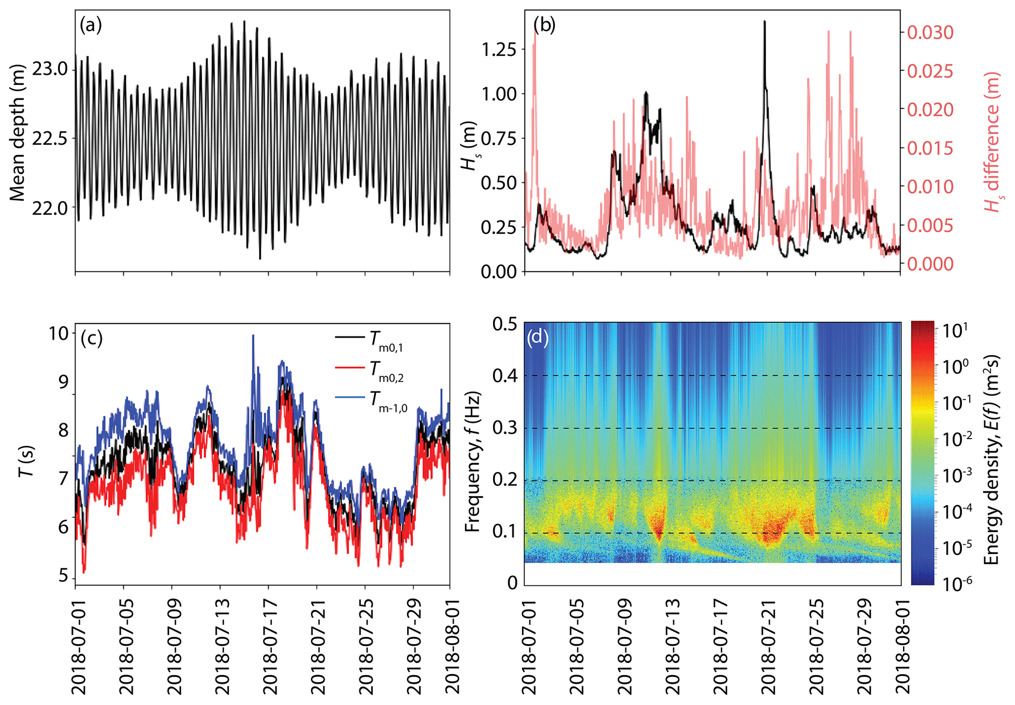
Figure 4 An example of outputs for 1 month (July 2018) of deployment HBK9: (a) mean depth $\stackrel{\mathrm{‾}}{z_{\text{lf}}}$; (b) primary y axis: significant wave height, H_s for f_max=∞, secondary y axis: the difference between H_s for f_max=∞ and for f_max=f_lastval; (c) wave period, T, for f_max=∞; (d) wave energy spectra E₀(f).

As A(f) quickly decreases with increasing wave frequency, the values of E₀(f) computed from Eq. (5) become unreliable for f higher than some limiting frequency f_lastval. Here, f_lastval was computed for each spectrum separately, based on a universal (constant for all spectra) limiting value of A: A_lim=0.05 (note that, consistent with the linear wave theory used throughout this analysis, the values of A depend only on water depth and frequency of a given spectral component but not on the amplitude of that component). That is, f_lastval is the highest frequency for which A>A_lim. For all f>f_lastval, a high-frequency tail of the form $E_{\mathrm{0}}\left(f\right)\sim f^{-\mathrm{4}}$ was added after Kaihatu et al. (2007) by extrapolating the trend from the last n=10 reliably estimated E₀(f) values (yellow line in Fig. 3):

$$\begin{array}{}\text{(8)}& E_{\mathrm{0}}\left(f\right)={\stackrel{\mathrm{̃}}{E}}_{\mathrm{0}}{f}^{-\mathrm{4}}\text{ for }f>f_{\text{lastval}},\end{array}$$

where

$$\begin{array}{}\text{(9)}& {\stackrel{\mathrm{̃}}{E}}_{\mathrm{0}}=\sum _{j=\mathrm{0}}^{n-\mathrm{1}}{E}_{\mathrm{0}}\left(f_{\text{lastval}-j}\right)f_{\text{lastval}-j}^{-\mathrm{4}}/\sum _{j=\mathrm{0}}^{n-\mathrm{1}}{f}_{\text{lastval}-j}^{-\mathrm{8}}.\end{array}$$

3.3 Mean wave parameters

In calculation of mean (integral) wave parameters, frequencies f<f_min = 0.04 Hz (corresponding to wave periods higher than 25 s) were ignored. This limit corresponds to the approximate boundary between wind-generated and infragravity waves, as well as to the lower-frequency limit typically used in spectral wave models (e.g. Holthuijsen, 2007). Thus, the mean wave parameters were computed for f_min < f < f_max. In the final dataset, two sets of those parameters are provided, referred to as observational one (for f_max = f_lastval) and modelled one (for f_max=∞). The spectral moments m_n of E₀(f) are defined as

$$\begin{array}{}\text{(10)}& m_n=\underset{f_{\text{min}}}{\overset{f_{\text{lastval}}}{\int }}{E}_{\mathrm{0}}\left(f\right)f^n\mathrm{d}f+C{\displaystyle \frac{\mathrm{1}}{\mathrm{3}-n}}{\stackrel{\mathrm{̃}}{E}}_{\mathrm{0}}{f}_{\text{lastval}}^{n-\mathrm{3}}\text{ for }n\in N,\end{array}$$

where ${\stackrel{\mathrm{̃}}{E}}_{\mathrm{0}}$ is computed from Eq. (9), C=0 if f_max = f_lastval and C=1 if f_max=∞. Based on m_n, the following wave parameters are calculated: the significant wave height H_s, the mean absolute wave period T_m0,1, the mean absolute zero-crossing period T_m0,2, and the so-called energy period $T_{\mathrm{m}-\mathrm{1},\mathrm{0}}$:

$$\begin{array}{}\text{(11)}& {\displaystyle }& {\displaystyle }{H}_{\mathrm{s}}=\mathrm{4}\sqrt{m_{\mathrm{0}}},\text{(12)}& {\displaystyle }& {\displaystyle }{T}_{\mathrm{m}\mathrm{0},\mathrm{1}}=m_{\mathrm{0}}/m_{\mathrm{1}},\text{(13)}& {\displaystyle }& {\displaystyle }{T}_{\mathrm{m}\mathrm{0},\mathrm{2}}=\sqrt{m_{\mathrm{0}}/m_{\mathrm{2}}},\text{(14)}& {\displaystyle }& {\displaystyle }{T}_{\mathrm{m}-\mathrm{1},\mathrm{0}}=m_{-\mathrm{1}}/m_{\mathrm{0}}.\end{array}$$

Table 2 Dataset content. “DepID” stands for deployment ID.

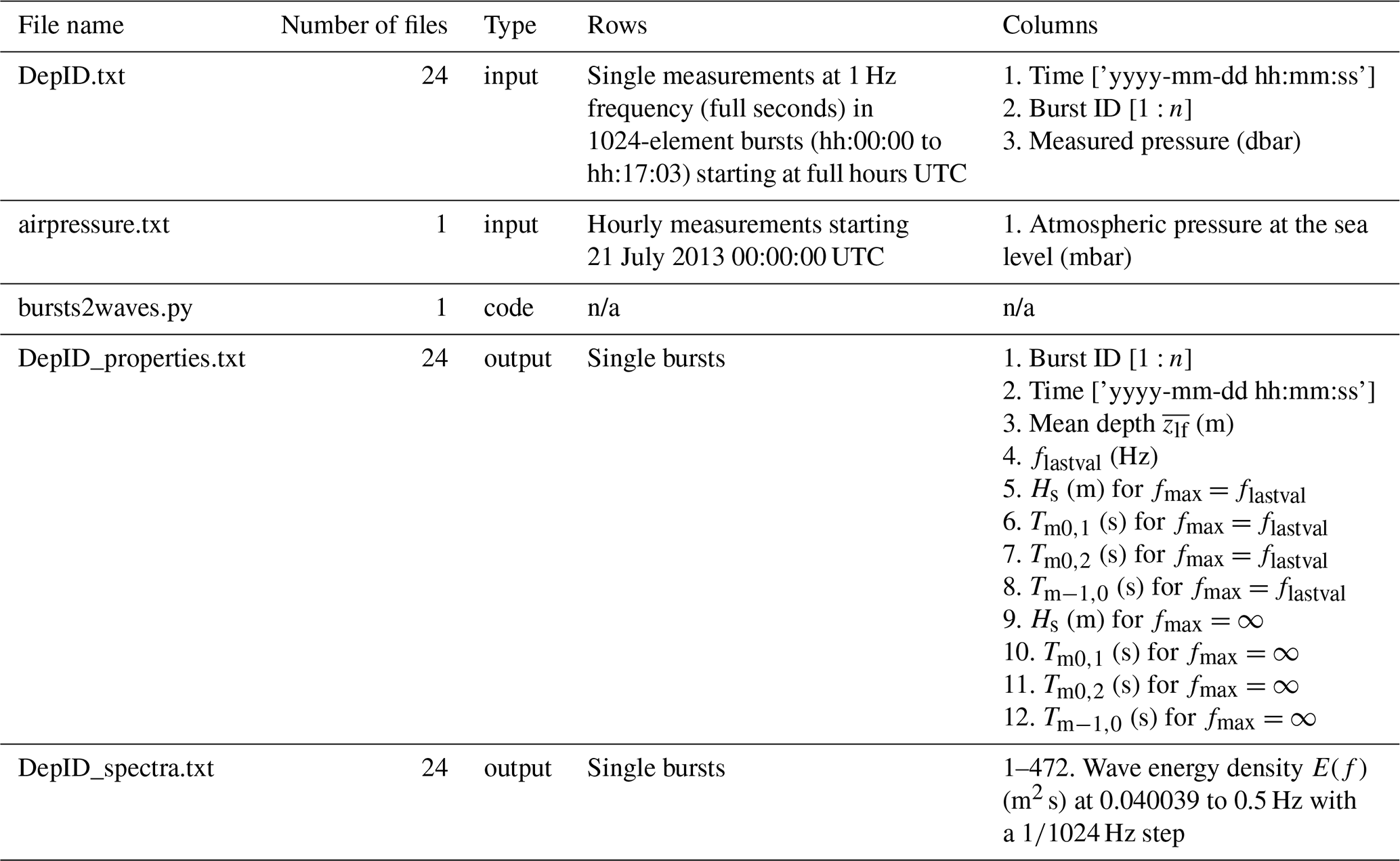
n/a: not applicable.

3.4 Output data

There are two output files for each deployment with rows representing bursts. The first one (“DepID_properties.txt”) contains the information on burst (number and time), mean water depth $\stackrel{\mathrm{‾}}{z_{\text{lf}}},f_{\text{lastval}}$, and the four mean wave parameters defined in Eqs. (11)–(14), in two versions, i.e. for C=0 and C=1, respectively, in Eq. (10). The second file provides wave energy spectra for frequencies from 0.040039 to 0.5 Hz with step Δf = $\frac{\mathrm{1}}{\mathrm{1024}}$ Hz (472 columns). Figure 4 provides a visualisation of an example 1-month period of data. Table 2 provides the dataset content (Swirad et al., 2023).

3.5 Quality control

The instruments remained at the seabed thanks to the anchor weight. However, a few times they were transported by ice or strong waves resulting in an abrupt change in mean depth visible in the output data (e.g. Fig. 5a). This situation occurred three times: in VES1 bursts no. 83 (depth rise of ∼ 1 m) and no. 370 (depth drop of ∼ 2.3 m) and in GAS5 burst no. 13 420 (depth rise of ∼ 0.7 m). In the case of VES1 burst no. 83 and GAS5 burst no. 13 420, it occurred in between bursts with no impact on calculated wave energy spectra and bulk parameters. Therefore, the data are left unchanged. If the dataset is used for tide analysis, time series should be split at the depth change event and treated separately. To identify erroneous bursts, we investigated the energy density for f < 0.5 Hz and identified two bursts with abnormally high energy density at low frequencies that resulted in erroneous calculation of bulk parameters (e.g. Fig. 5b): VES1 burst no. 370 and HBK1 burst no. 44. In the first case, the error resulted from instrument displacement during the burst. In the second case, mean depth rose by ∼ 0.5 m, remained higher for a few hours and dropped back to a typical level. There was no anomaly in atmospheric pressure and we speculate that the artefact may be due to the presence of glacier ice at the sea surface. In both cases, we replaced all output wave parameters with “NaN” (not a number).

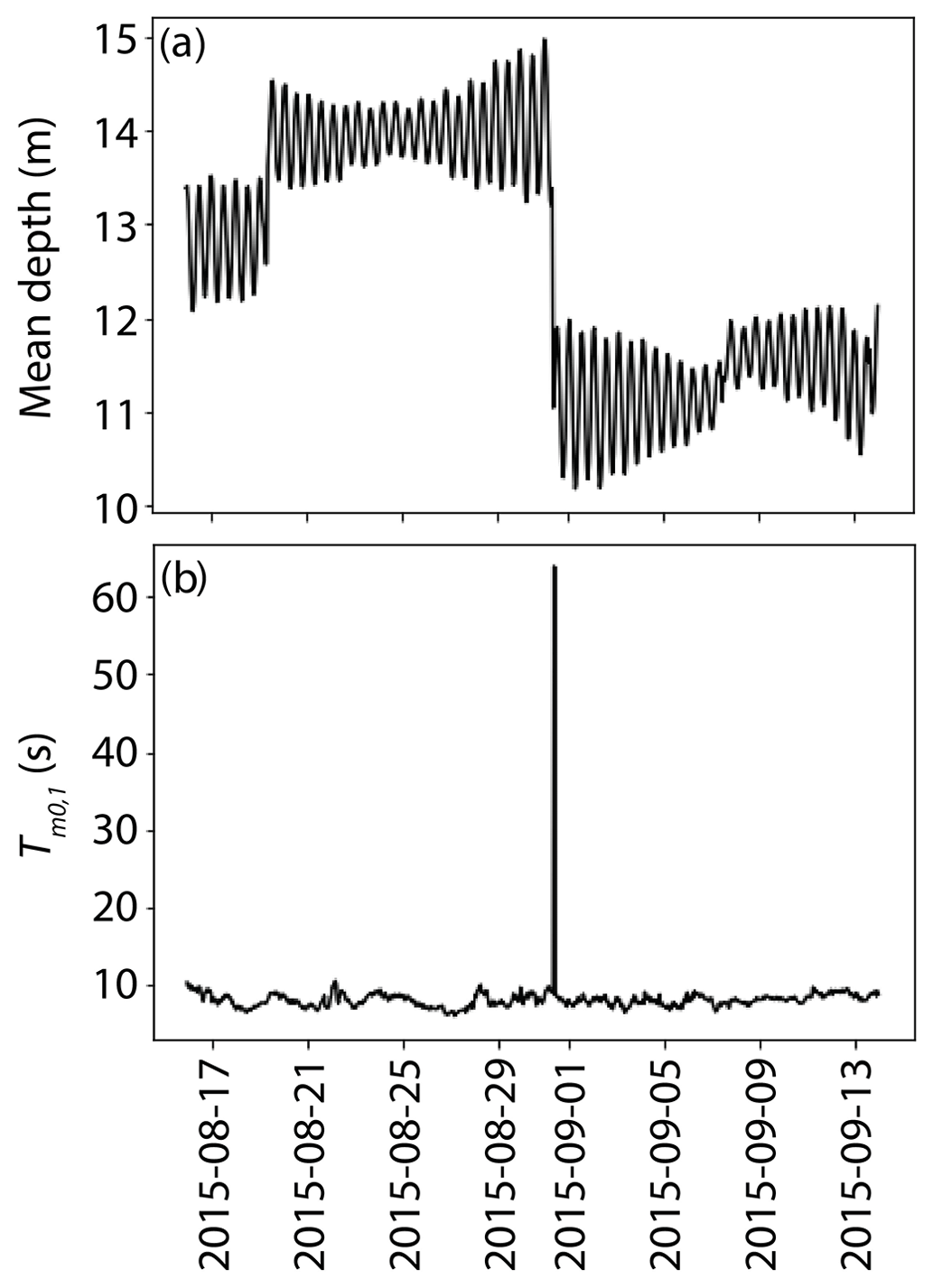
Figure 5 An example of data errors for deployment VES1: (a) mean depth $\stackrel{\mathrm{‾}}{z_{\text{lf}}}$; (b) mean wave period T_m0,1 for f < 0.5 Hz.

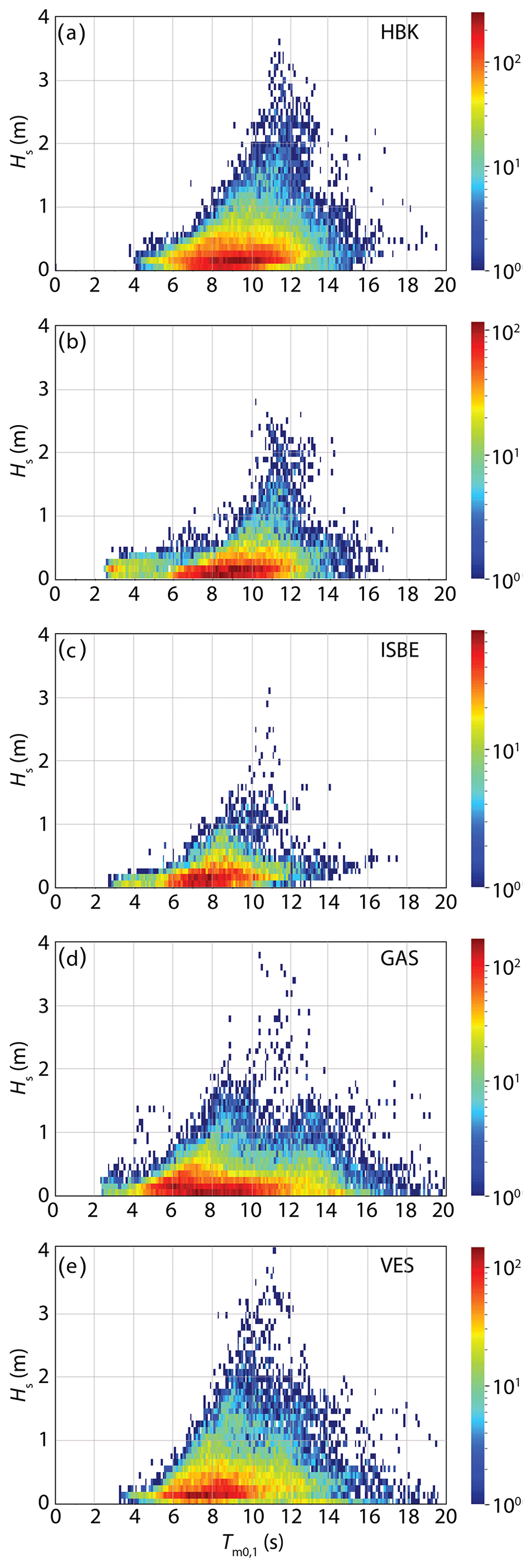
Figure 6 Distribution of significant wave height, H_s (y axis; range: 0–4 m with 0.1 m bins) and mean absolute wave period, T_m0,1 (x axis; range 0–20 s with 0.1 s bins) with f_max=∞ for (a) Hansbukta (HBK), (b) western Isbjørnhamna (ISBW), (c) eastern Isbjørnhamna (ISBE), (d) Gåshamna (GAS), and (e) Veslebogen (VES).

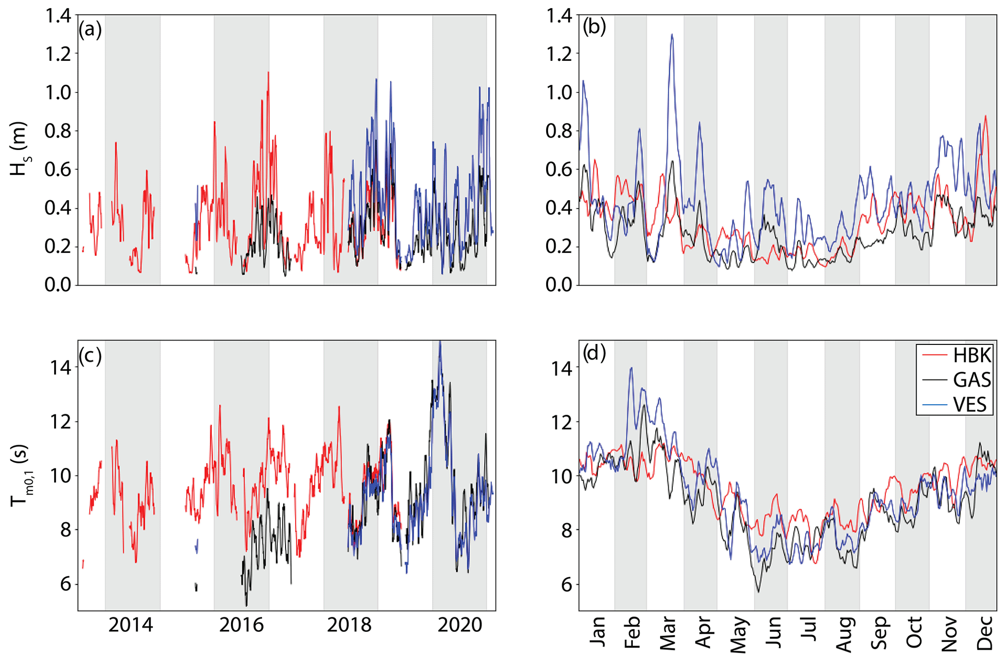
Figure 7 Summary of the wind wave characteristics for Hansbukta (HBK), Gåshamna (GAS) and Veslebogen (VES) for f_max=∞: (a) mean daily significant wave height, H_s, smoothed with a 15 d moving average; (b) mean daily significant wave height, H_s, for days of year smoothed with a 5 d moving average; (c) mean daily absolute wave period, T_m0,1, smoothed with a 15 d moving average; (d) mean daily absolute wave period, T_m0,1, for days of year smoothed with a 5 d moving average.

Table 3 Summary of significant wave height (H_s: mean, 99th percentile for the full dataset and by quarters of the year) and mean full dataset wave period (mean absolute wave period T_m0,1, mean absolute zero-crossing period T_m0,2, and energy period $T_{\mathrm{m}-\mathrm{1},\mathrm{0}}$). HBK = Hansbukta, ISB = Isbjørnhamna (W = western, E = eastern), GAS = Gåshamna, VES = Veslebogen. Rettkvalbogen (RET) is excluded as the 13 d duration is not sufficient to derive seasonal statistics.

4 Results

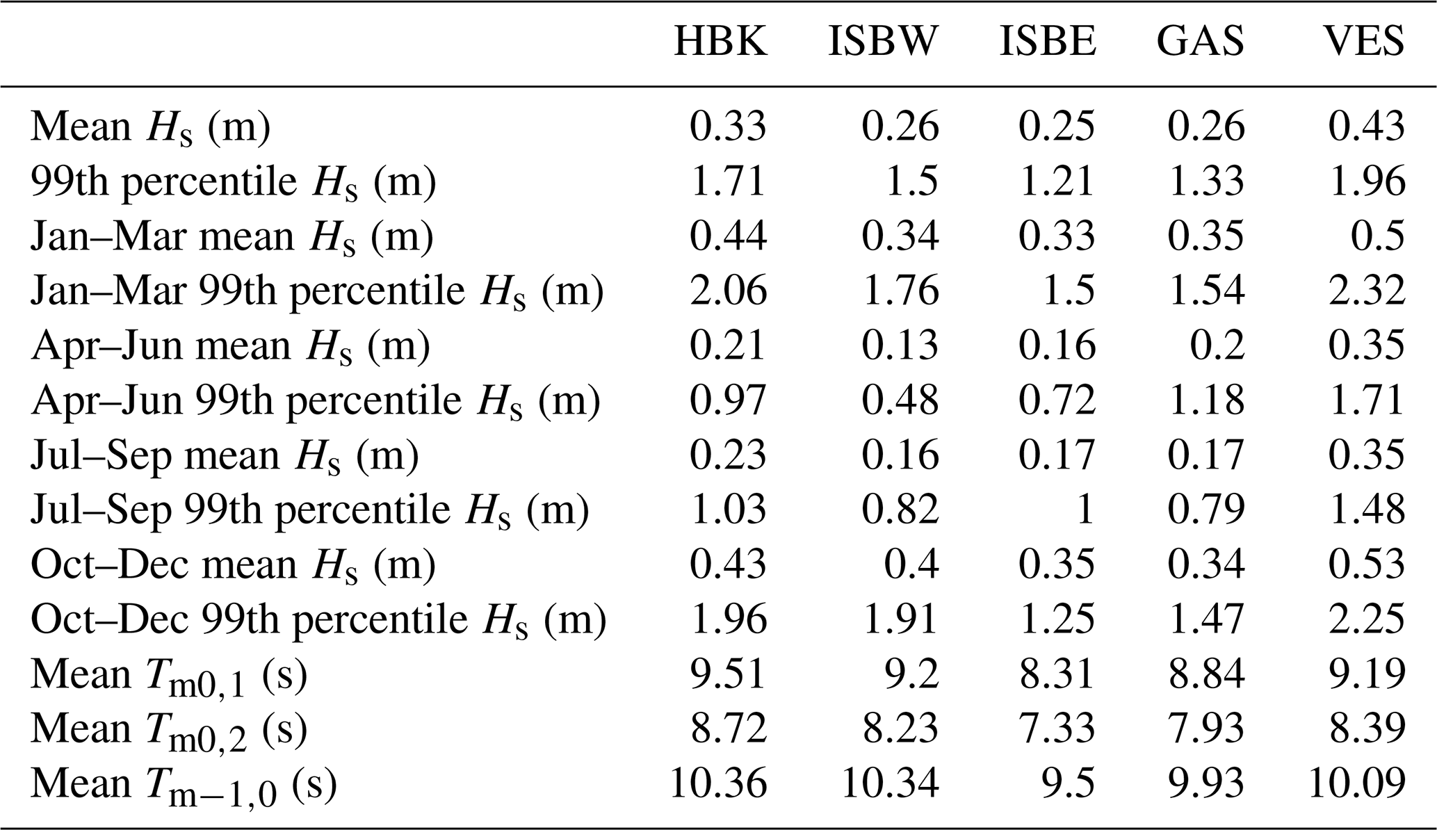
For all bays except Rettkvalbogen, time series length exceeded 1 year, providing information on seasonal variability in wind wave conditions. The largest waves characterise Veslebogen, the western-most of the analysed northern bays (Fig. 6). Mean full dataset H_s ranged from 0.25 m in eastern Isbjørnhamna to 0.43 m in Veslebogen, and respective 99th percentile H_s values equalled 1.21 and 1.96 m. Waves were the highest in the first and last quarters of the year with the highest mean H_s of 0.53 m in October–December and 99th percentile H_s of 2.32 m in January–March, both in Veslebogen (Table 3). A seasonal trend is also clearly visible in Fig. 7. Winter months are characterised by generally higher and longer waves, a finding consistent with the multi-decadal wave model reanalysis of Wojtysiak et al. (2018) for open Greenland Sea, west of Hornsund.

5 Data availability

The inputs, outputs and the Python code described in this paper are available in the PANGAEA repository (https://doi.org/10.1594/PANGAEA.954020; Swirad et al., 2023). Raw data downloaded from the instruments are part of the IG PAS LONGHORN oceanographic monitoring, and they are available at the IG PAS Data Portal (https://doi.org/10.25171/InstGeoph_PAS_IGData_NBP_2022_005; Swirad et al., 2022). As the monitoring programme is on-going, future raw data and data processed in the same way as described here will be uploaded to the IG PAS Data Portal (https://dataportal.igf.edu.pl/, last access: 26 June 2023).

6 Summary

We present the first multi-year continuous wind wave and water level dataset for Hornsund fjord, Svalbard. Twenty four single deployments of underwater RBR sensors at 8–23 m depth between July 2013 and February 2021 were used to measure water levels in five bays of northern Hornsund (Hansbukta, western Isbjørnhamna, eastern Isbjørnhamna, Rettkvalbogen, Veslebogen) and one of southern (Gåshamna) Hornsund. Raw data (Swirad et al., 2022) were subsampled to 1024 s sets (∼ bursts) at 1 Hz measurement interval at 1 h burst interval, and they were then used to derive mean water levels, wave spectra and bulk wave parameters. We describe the procedure (available also as a Python code) that includes subtracting atmospheric pressure, depth calculation, fast Fourier transform, correction for the decrease of the wave orbital motion with depth and adding a high-frequency tail. We performed quality control on the output data. The dataset can be used to, for example, characterise wind wave climate in Hornsund; identify seasonal to inter-annual trends; calibrate and validate wave models (as shown by Herman et al., 2019); and facilitate analysis of sea-ice impact on wave attenuation, empirical modelling of wave run-up on Arctic beaches, and predicting future change. We provide individual bursts with pressure time series and the code for the users to apply different analysis methods, use alternative algorithm parameters, analyse non-linear effects, etc., depending on the application.