OceanSODA-UNEXE: a multi-year gridded Amazon and Congo River outflow surface ocean carbonate system dataset

Large rivers play an important role in transferring water and all of its constituents, including carbon in its various forms, from the land to the ocean, but the seasonal and inter-annual variations in these riverine flows remain unclear. Satellite Earth observation datasets and reanalysis products can now be used to observe synoptic-scale spatial and temporal variations in the carbonate system within large river outflows. Here, we present the University of Exeter (UNEXE) Satellite Oceanographic Datasets for Acidification (OceanSODA) dataset (OceanSODA-UNEXE) time series, a dataset of the full carbonate system in the surface water outflows of the Amazon (2010–2020) and Congo (2002–2016) rivers. Optimal empirical approaches were used to generate gridded total alkalinity (TA) and dissolved inorganic carbon (DIC) fields in the outflow regions. These combinations were determined by equitably evaluating all combinations of algorithms and inputs against a reference matchup database of in situ observations. Gridded TA and DIC along with gridded temperature and salinity data enable the calculation of the full carbonate system in the surface ocean (which includes pH and the partial pressure of carbon dioxide, pCO₂). The algorithm evaluation constitutes a Type-A uncertainty evaluation for TA and DIC, in which model, input and sampling uncertainties are considered. Total combined uncertainties for TA and DIC were propagated through the carbonate system calculation, allowing all variables to be provided with an associated uncertainty estimate. In the Amazon outflow, the total combined uncertainty for TA was 36 µmol kg⁻¹ (weighted root-mean-squared difference, RMSD, of 35 µmol kg⁻¹ and weighted bias of 8 µmol kg⁻¹ for n = 82), whereas it was 44 µmol kg⁻¹ for DIC (weighted RMSD of 44 µmol kg⁻¹ and weighted bias of −6 µmol kg⁻¹ for n = 70). The spatially averaged propagated combined uncertainties for the pCO₂ and pH were 85 µatm and 0.08, respectively, where the pH uncertainty was relative to an average pH of 8.19. In the Congo outflow, the combined uncertainty for TA was identified as 29 µmol kg⁻¹ (weighted RMSD of 28 µmol kg⁻¹ and weighted bias of 6 µmol kg⁻¹ for n = 102), whereas it was 40 µmol kg⁻¹ for DIC (weighted RMSD of 37 µmol kg⁻¹ and weighted bias of −16 µmol kg⁻¹ for n = 77). The spatially averaged propagated combined uncertainties for pCO₂ and pH were 74 µatm and 0.08, respectively, where the pH uncertainty was relative to an average pH of 8.21. The combined uncertainties in TA and DIC in the Amazon and Congo outflows are lower than the natural variability within their respective regions, allowing the time-varying regional variability to be evaluated. Potential uses of these data would be the assessment of the spatial and temporal flow of carbon from the Amazon and Congo rivers into the Atlantic and the assessment of the riverine-driven carbonate system variations experienced by tropical reefs within the outflow regions. The data presented in this work are available at https://doi.org/10.1594/PANGAEA.946888 (Sims et al., 2023).

1 Introduction

Rivers connect the land and ocean, providing a major pathway for carbon transport to the ocean (Regnier et al., 2013). The inorganic carbon content of rivers is poorly constrained because it is difficult to sufficiently sample these highly spatiotemporally variable river outflows. Global estimates of the riverine flow of carbon from the land to the ocean (Friedlingstein et al., 2022) are determined from in situ upscaling (Regnier et al., 2013), ocean inverse model estimates (Jacobson et al., 2007), partial pressure of carbon dioxide (pCO₂) ocean-sink-based estimates (Watson et al., 2020) and atmosphere-inversion-based estimates (Rödenbeck et al., 2018). Clearly, new methods that improve the characterization of the magnitude, variability and temporal variations in carbon transported by rivers will help constrain uncertainties within global carbon budgets (Hauck et al., 2020).

The vast majority of pCO₂ measurements in the Surface ocean CO₂ Atlas (SOCAT) were made on research ships and ships of opportunity that mainly survey the open ocean and continental shelves (Bakker et al., 2016). Many bottle samples have been collected for total alkalinity (TA) and dissolved organic carbon (DIC) in rivers, but fully surveying the entirety of large rivers across all seasons is logistically challenging, requiring extensive and economically expensive field campaigns (Ward et al., 2017). For example, the majority of the largest 100 rivers by discharge are found in South America and Asia (Dai and Trenberth, 2002) and have been historically under-sampled for carbonate system variables (Laruelle et al., 2015). Issues related to the scarcity of measurements are compounded by insufficient knowledge of the hydrology and spatial area extents of these systems (Allen and Pavelsky, 2018). Additionally, the amount of carbon in the rivers is a function of runoff rates, rainfall and land use, all of which have been disrupted by climate change and land use change (Piao et al., 2007; Kaushal et al., 2014; Regnier et al., 2013). This lack of large-spatial-scale and large-temporal-scale baseline carbonate system observations in rivers means that assessing changes in these systems is challenging.

The carbon dynamics of the world's rivers also have implications for local biogeochemistry. Ocean acidification is the long-term process by which the oceans absorb atmospheric CO₂; this process makes oceans less alkaline (due to an increase in the hydrogen ion concentration), lowers their pH and decreases their carbonate ion availability (Doney et al., 2009). Ocean acidification poses a threat to marine organisms that build calcium carbonate structures, and many rivers are sensitive to this due to their low buffering capacity (Hu and Cai, 2013; Cai et al., 2011). River plumes can negatively influence wild fisheries and the aquaculture industry (Mathis et al., 2015; Cattano et al., 2018), as plumes can transport low-pH waters with the ability to impact the growth and life stages of many marine organisms (Cai et al., 2021). Additionally, river plumes can interact with high-biodiversity regions that are quick to respond to sudden changes in the carbonate system, such as sensitive coral reef systems (Mongin et al., 2016; Dong et al., 2017). Intermittent changes in the carbonate system caused by river plumes can potentially jeopardize ecosystem services like fisheries, aquaculture and shoreline protection, and the resultant financial and biodiversity losses are of great interest to local communities, businesses and policymakers (Doney et al., 2020).

Satellite Earth observations provide a means of accurately assessing the carbonate content of large rivers by using satellite-observed oceanographic variables with published empirical algorithms that link carbonate system variables to the satellite-derived variables (Land et al., 2019). The Satellite Oceanographic Datasets for Acidification (OceanSODA) project (https://esa-oceansoda.org, last access: 10 August 2022) was established to further develop these approaches. We present the University of Exeter (UNEXE) OceanSODA dataset (OceanSODA-UNEXE), which comprises decadal datasets of riverine carbonate system variables for the two largest rivers in the world by discharge, the Amazon and the Congo (Dai and Trenberth, 2002). This paper details how the optimal combinations of empirical algorithms and Earth observation datasets were selected and used to construct OceanSODA-UNEXE. It also provides an assessment of the uncertainty associated with the key TA and DIC parameters using a standardized uncertainty framework and a large in situ database. The remaining ocean carbon system variables were calculated from TA and DIC with propagated uncertainties.

2 Methods

2.1 Statistical terms overview

Root-mean-squared difference (RMSD) is a measure of accuracy and is calculated as the square root of the average of squared errors, e.g. RMSD = $\left(\right(\mathrm{\Sigma }(x_{\mathrm{0}}-x_{\mathrm{1}}{)}^{\mathrm{2}})/n{)}^{\mathrm{1}/\mathrm{2}}$, where x₀ denotes the estimated values, x₁ denotes the reference values and n is the number of observations. The bias of a dataset is defined as the mean difference between the estimation and reference, Bias = $\mathrm{\Sigma }(x_{\mathrm{0}}-x_{\mathrm{1}}))/n$. The mean absolute difference (MAD) of a dataset is a measure of variability and is calculated as MAD = $(\mathrm{\Sigma }\mathrm{|}x-\stackrel{\mathrm{‾}}{x}\mathrm{|})/n$, where $\stackrel{\mathrm{‾}}{x}$ is the mean. The correlation coefficient (r_ij) is a measure of linear correlation between the estimate and the reference variables and is defined as r_ij = $\left(\mathrm{\Sigma }\right(x_i-{\stackrel{\mathrm{‾}}{x}}_i\left)\right(x_j-{\stackrel{\mathrm{‾}}{x}}_j\left)\right)/\left(\mathrm{\Sigma }\right(x_i-{\stackrel{\mathrm{‾}}{x}}_i{)}^{\mathrm{2}}\mathrm{\Sigma }(x_j-{\stackrel{\mathrm{‾}}{x}}_j{)}^{\mathrm{2}}{)}^{\mathrm{1}/\mathrm{2}}$. Uncertainty representation and the terminology used throughout this paper are consistent with the International Bureau of Weights and Measures (BIPM) Guide to the expression of uncertainty in measurement (GUM) methodology (JCGM, 2008).

Weighted statistics allow uncertainties in the reference dataset (in situ measurement uncertainty in this case) to be accounted for within the performance analysis (i.e. the reference data are not considered “truth”, as they also contain uncertainties). Weights are calculated as the sum of the individual weight of each algorithm (w), where w = $\mathrm{1}/\left(\right(\text{in situ measurement uncertainty}{)}^{\mathrm{2}}$ + $(\text{literature algorithm uncertainty}{)}^{\mathrm{2}}{)}^{\mathrm{1}/\mathrm{2}}$ (Ford et al., 2021). For clarity and easy comparison to previous published work, both weighted and unweighted statistics of all metrics are given, e.g. weighted RMSD (wRMSD) is calculated as wRMSD = $\left(\mathrm{\Sigma }\right({\text{weights}}^{\ast }(x_{\mathrm{0}}-x_{\mathrm{1}}{)}^{\mathrm{2}}))$.

When evaluating algorithms using a statistical measure, in this case wRMSD, a further issue can arise where the valid region over which each algorithm can be applied overlaps with different in situ data. For example, an algorithm evaluated using data from highly variable coastal waters may have a higher wRMSD than another algorithm evaluated solely using data from a less variable open-ocean region; in this scenario, it may be falsely concluded that the coastal ocean algorithm performs worse. This is a clear weakness of comparing wRMSD values from different sources and across differing regions (Land et al., 2019). Following the methodology of Land et al. (2019) we calculate RMSDe using the wRMSD result; RMSDe is a more representative metric to compare accuracies, as it allows algorithms to be evaluated in a like-for-like manner, enabling their performance to be ranked. It is important to note that wRMSD = RMSDe for the best algorithm, as the best algorithm will always have a score of one. To ensure the robustness of any statistics generated, it was considered prudent to specify a minimum data threshold. Only algorithms that had at least 30 matchups (n = 30) between the algorithm and reference outputs were used in the calculation of RMSDe; this was done to prevent the selection of algorithms with low RMSDe values caused by evaluating the algorithm with a small number of data points. The wRMSD is used as the preferred measure of accuracy in this paper, but unweighted RMSD values are also given.

2.2 Selection of empirical algorithms

In order to generate the full ocean carbonate system, two of the four carbonate system variables are needed. As TA is closely linked to salinity, it is selected as one variable; DIC is selected as the second variable. There are many algorithms in the published literature for both TA and DIC, and the required measurements in the river outflows are also available to evaluate those algorithms. Other pairings of carbonate system parameters can be used to derive the full carbonate system (Land et al., 2015) but are not explored here – for example, Gregor and Gruber (2021) use TA and pCO₂.

An exhaustive literature search using 24 search terms identified prospective algorithms that could be applied to the Amazon and Congo River outflows. The full list of search terms and identified algorithms can be found in the Supplement. The regional bounds of the Amazon outflow were defined as being 2^∘ S–24^∘ N and 70–31^∘ W. The bounds of the Congo outflow were defined as being between 10^∘ S–4^∘ N and 2^∘ W–16^∘ E. To be included in the algorithm evaluation, algorithms needed to be applicable to these regions and to take the form of a linear or quadratic relationship with input variables that were easy to obtain and were available as spatially and temporally varying datasets. These input variables included sea surface temperature (SST), sea surface salinity (SSS), potential temperature (which is assumed to be approximately equal to SST at the surface), dissolved oxygen (DO), nitrate (${\mathrm{NO}}_{\mathrm{3}}^{-}$), phosphate (${\mathrm{PO}}_{\mathrm{4}}^{-\mathrm{3}}$), silicate (${\mathrm{SiO}}_{\mathrm{4}}^{-\mathrm{4}}$) and chlorophyll a. A total of 26 of the identified algorithms were not included in the algorithm evaluation, as they could not generate TA or DIC using the accessible input variables listed above or were not based on empirical algorithms (see Table S2 in the Supplement for the full list). Any approaches involving biogeochemical models or neural networks were not included in the algorithm evaluation. A total of 10 TA algorithms (5 of 10 report RMSD values in their original publication) and 6 DIC algorithms (5 of 6 report RMSD) were evaluated for the Amazon, whereas 4 TA algorithms (3 of 4 report RMSD) and 9 DIC algorithms (4 of 7 report RMSD) were evaluated for the Congo (Table S1 in the Supplement). The wRMSD and RMSDe can only be calculated for algorithms that report RMSD, so it is important to distinguish these. Table S1 details each algorithm's input variables, the published algorithm RMSD, the stated environmental ranges for which the algorithm is valid and some brief descriptive notes of how the algorithm was developed. The target output variable, the input variables, the mathematical algorithm, the valid geographical region and the valid geophysical conditions for each algorithm were then gathered for use in the algorithm evaluation process.

2.3 Algorithm evaluation

A multipurpose global reference matchups database (MDB), matching in situ carbonate system parameters from the surface 10 m with satellite, model and interpolated in situ datasets, was used to perform the algorithm evaluation (Land et al., 2023). The MDB is optimized to reduce biases arising from uneven data density; this is achieved by grouping in situ observations into 100 km diameter regions of interest (ROI) which span a 10 d time period. The MDB was constructed from global datasets that include all of the variables required for all algorithms (SST, SSS, θ, DO, ${\mathrm{NO}}_{\mathrm{3}}^{-}$, ${\mathrm{PO}}_{\mathrm{4}}^{-\mathrm{3}}$, ${\mathrm{SiO}}_{\mathrm{4}}^{-\mathrm{4}}$ and chlorophyll a; see Sect. 2.2). The MDB includes three global SST datasets – the European Space Agency Climate Change Initiative SST (ESACCI SST) v2.1 (Merchant et al., 2019; Good et al., 2019), Optimum Interpolation SST (OISST) v2.1 (Huang et al., 2021; Banzon et al., 2016) and the Coriolis Ocean dataset for Reanalysis (CORA) v5.2 (Szekely et al., 2019) – and four global SSS datasets – the European Space Agency Climate Change Initiative SSS (ESACCI SSS) v2.31 (Boutin et al., 2020, 2021), CORA v5.2 (Szekely et al., 2019), the In Situ Analysis System 15 (ISAS15) (Kolodziejczyk et al., 2021; Gaillard et al., 2016) and the Remote Sensing Systems data from the Soil Moisture Active Passive satellite (RSS-SMAP) level 3 v4.0 (Meissner et al., 2019, 2018). The MDB also contains TA, DIC and pH values, most of which come from the Global Ocean Data Analysis Project (GLODAPv2.2020) database (Olsen et al., 2016), and pCO₂ values, most of which come from SOCAT v2020 (Bakker et al., 2016), along with additional data for Arctic waters. A full list of references for data variable sources used in the MDB can be found in Land et al. (2023). Before beginning this analysis, we limited our analysis to only use MDB data that fall within the following bounds: SST > −10 or < 40 ^∘C, SSS > 0 or < 50, DIC > 500 or < 3000 µmol kg⁻¹, TA > 500 or < 3000 µmol kg⁻¹, pH > 6 or < 8.5, and pCO₂ > 100 or < 3000 µatm. These constraints are consistent with the conditions likely within the Amazon and Congo regions.

Each valid algorithm was implemented by closely following the specific literature recommendations; this was done in such a way that empirical algorithms were only assessed for the geographical and geophysical ranges for which they were originally developed. The algorithm evaluation involved running each algorithm with inputs from the MDB to estimate the TA and DIC outputs (termed the “algorithm output”). Each algorithm output was then evaluated using the TA and DIC values from the MDB matchup database (termed the “reference output”). The RMSD, bias, correlation coefficient and MAD are calculated from the algorithm output and the reference output. Additionally, wRMSD was calculated for algorithms for which an RMSD is reported in the literature. Where a wRMSD was calculated and the matchups (n) were > 30, an RMSDe was calculated for those algorithms following the methodology of Land et al. (2019). As the MDB includes three global SST and four global SSS datasets, each algorithm was run for each of the 12 combinations of SST and SSS input datasets, and separate statistics were generated for each configuration. The subset of input variables from the MDB used to implement the algorithm, the algorithm output and the reference output for all 12 SST and SSS combinations are included in the Supplement. Additionally, summary statistics between the algorithm output and the reference output are also provided in the Supplement; these statistics are the mean, the weighted mean (wmean), the standard deviation, the RMSD, the weighted RMSD (wRMSD), the RMSDe, the Bias, the weighted Bias (wBias), r, the weighted r (wr), the MAD and the weighted MAD (wMAD).

The best performing TA and DIC algorithms for both regions were determined by ranking the algorithms by RMSDe: the best performing algorithms were the algorithms with the lowest RMSDe values. In order to select algorithms suitable for generating time series, observation datasets for SSS and SST needed a temporal overlap of at least 8 years. The remainder of this paper exclusively discusses the time series generated with these “optimal algorithms”.

The algorithm evaluation process follows a standardized framework for a Type-A uncertainty evaluation for TA and DIC, whereby the following sources of uncertainties are considered:

1. the TA or DIC measurement uncertainty – measurement uncertainty for both TA and DIC is typically stated as ± 4 µmol kg⁻¹, but (following Bockmon and Dickson, 2015) we used a more conservative measurement uncertainty of ± 10 µmol kg⁻¹ (approximately equal to 0.5 % of the nominal TA and DIC values for the open ocean);

2. the algorithm uncertainty – the RMSD stated in the literature for each algorithm;

3. the spatial uncertainty – uncertainty arising from spatial heterogeneity in the region;

4. the uncertainty due to differences in the measurement depths in the MDB.

The measurement uncertainty of 10 µmol kg⁻¹ and the algorithm uncertainty are explicitly considered in the calculated wRMSD, and the remaining uncertainties should be minimized by using the MDB, which was designed to reduce these components (Land et al., 2023). Accounting for all known sources of uncertainty constitutes a complete Type-A uncertainty evaluation. The combined standard uncertainty (δQ) for TA and DIC is calculated as δQ = $\left(\right(\mathit{\delta }a{)}^{\mathrm{2}}+(\mathit{\delta }b{)}^{\mathrm{2}}{)}^{\mathrm{1}/\mathrm{2}}$, where δa is the RMSDe from the evaluation algorithm and δb is the wBias. The uncertainty estimates provided within the dataset are the combined standard uncertainty (δQ), and these combined standard uncertainties are reported without confidence intervals.

To aid in the interpretation of the combined uncertainty budgets, a second Type-A uncertainty evaluation of the TA and DIC approaches was calculated based purely on the empirical algorithm (e.g. literature RMSD value) and the uncertainties in the input data propagated using standard techniques (Taylor, 1997) and assuming that any uncertainties were uncorrelated. This is a second independent Type-A uncertainty evaluation that does not include uncertainties due to spatial variability and depth. Assuming that the first Type-A uncertainty evaluation has captured all of the uncertainties, the difference between the two uncertainty evaluations enables the estimation of the contribution of the spatial and depth variability to the uncertainty budget. A similar technique was recently used by Gregor and Gruber (2021), who referred to these two approaches as “top-down” (our first Type-A uncertainty evaluation) and “bottom-up” (our second Type-A uncertainty evaluation) assessments.

Evaluating each algorithm exactly as it appears in the literature is required to ensure equitably in the algorithm evaluation. Theoretically, all of the algorithms could have been modified to account for long-term changes in environmental conditions (e.g. oceanic CO₂ uptake and increased freshwater input to the oceans) in these two outflow regions that have likely occurred since the algorithms were first developed. However, accounting for changing environmental conditions is not straightforward. Whilst secular trends for variables like surface CO₂ are accurate for the open ocean, these regions are heavily impacted by the river outflows; therefore, applying open-ocean secular trends to these riverine regions is likely problematic and is considered beyond the scope of this study. The impact of any secular trends in any parameters is somewhat mitigated as the analysis focuses on the use of TA and DIC because these variables are likely less impacted by secular trends than pCO₂ and pH.

2.4 Creation of a gridded monthly time series product

The full-spatiotemporal-resolution SST and SSS datasets and gridded World Ocean Atlas (WOA) DO, ${\mathrm{NO}}_{\mathrm{3}}^{-}$, ${\mathrm{PO}}_{\mathrm{4}}^{-\mathrm{3}}$ and ${\mathrm{SiO}}_{\mathrm{4}}^{-\mathrm{4}}$ datasets were downloaded from their online repositories. The total size of these full-resolution datasets occupies ∼ 500 GB of hard drive space and take several days to fully download. The SST and SSS datasets were uncompressed and were regridded onto a monthly 1^∘ × 1^∘ standard World Geodetic System grid for use in creating the gridded output; the grid has 180^∘ of latitude and 360^∘ of longitude with 0^∘ centred on the Greenwich meridian. Reformatting the datasets considerably reduced the file size to a more manageable ∼ 50 GB. The scripts used to download these SST and SSS monthly datasets are fully automated, meaning that new data can easily be incorporated into future versions of OceanSODA-UNEXE.

For each target variable (TA or DIC), the selected optimal SST and SSS gridded datasets and gridded WOA datasets were used as inputs for the respective TA and DIC algorithms. The algorithms were applied to the datasets in the two outflow regions where the SST and SSS datasets overlapped in time for the published environmental limits of each algorithm. The monthly SST and SSS inputs as well as the calculated monthly output variable (TA or DIC) are saved to a netCDF4 file as separate variables on the grid described above with dimensions of 768 × 180 × 360. The time dimension is the number of months since January 1957. It is important to note that TA and DIC datasets (even if for the same region) can span different temporal domains and should, therefore, be treated as separate datasets. These differences are due to differences in the temporal range of the input data used to calculate them.

The oceanic carbon system equations (Millero, 2000) can be solved computationally (Lewis et al., 1998) using numerical software packages (Orr et al., 2015), and the established CO2SYS software package is now available in Python as PyCO2SYS (Humphreys et al., 2022). Where there was temporal overlap between TA and DIC in each region, the remaining oceanic carbonate system variables (pCO₂ and pH) were calculated using PyCO2SYS v1.71 (Humphreys et al., 2022). A number of other output variables were also calculated including fCO₂, the carbonate ion content (${\mathrm{CO}}_{\mathrm{3}}^{-\mathrm{2}}$), the bicarbonate ion content (${\mathrm{HCO}}_{\mathrm{3}}^{-}$), the hydrogen ion content (H⁺), and the calcite (Ω calcite) and aragonite (Ω aragonite) saturation states. PyCO2SYS was run with the selected optimal dataset (SST, SSS and WOA datasets where applicable, with the same data used for input and output conditions) at the surface (0 m depth) with the carbonic acid dissociation constants of Mehrbach et al. (1973) refitted by Dickson and Millero (1987) and the hydrogen sulfate dissociation constant of Dickson (1990). The full carbonate system is calculated twice: once using the optimal SST and SSS datasets that were used to calculate TA and then again employing those used to calculate DIC. Consequently, each netCDF file contains a complete set of carbonate system outputs that are unique to that specific input dataset.

Whilst some of the SST and SSS products used to create the gridded datasets contain only satellite-observed SST at a specified depth, some of the reanalysis SST and SSS products also incorporate surface ocean measurements from ships and buoys that were made at differing depths. The TA and DIC data used to generate the MDB come from the top 10 m of the ocean and have not been adjusted for potential concentration gradients in the surface ocean (Land et al., 2023). For these reasons, OceanSODA-UNEXE is deemed relevant in the surface 10 m of the ocean.

2.5 Uncertainties in the gridded monthly time series product

As stated in Sect. 2.3, the assessed combined standard uncertainties for TA and DIC are single fixed values provided as regionally static non-spatially varying fields in the netCDF files. Uncertainty information for SST and SSS is taken from the literature references and is provided as spatially varying fields in the netCDF. Uncertainties in TA, DIC, SST and SSS are provided as optional uncertainty input arguments in PyCO2SYS to generate uncertainties for pH, pCO₂, Ω calcite and Ω aragonite. PyCO2SYS uses a forward-finite-difference approach to calculate the derivatives needed to propagate uncertainties for all of these output variables. This produces a spatially varying combined uncertainty budget for each remaining carbonate system parameter. The spatially varying uncertainties in SST, SSS, pH, pCO₂, Ω calcite and Ω aragonite are all provided in the respective netCDF files.

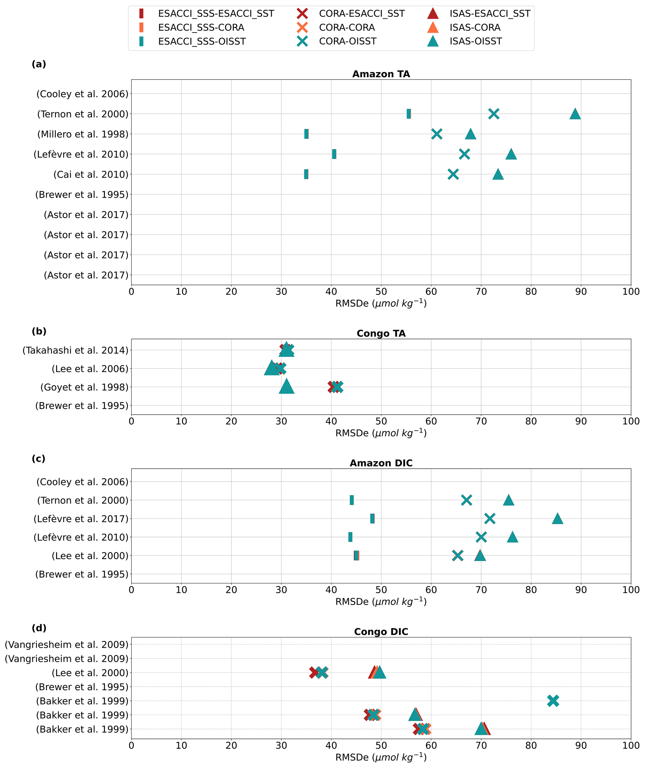
Figure 1 Results of the algorithm evaluation; the DIC and TA algorithms for the Amazon and Congo regions are compared by RMSDe. Each of the valid algorithms is listed by literature reference on the y axis, all of which correspond to algorithms in Table S1. Each SST and SSS dataset input configuration for which algorithms were evaluated is shown for each algorithm, with each SSS dataset given by a different symbol and each SST dataset given as a different colour in the legend. Entries are blank if there was no RMSD value in the literature, if there were < 30 matchups or if the assessed RMSDe value was > 100 µmol kg⁻¹.

Table 1 Summary table of the best combination of algorithm and SST/SSS datasets (aka the “optimal algorithms”) in the Amazon River domain. These optimal algorithms were determined by selecting the algorithm with the lowest RMSDe where there was at least 8 years of data.

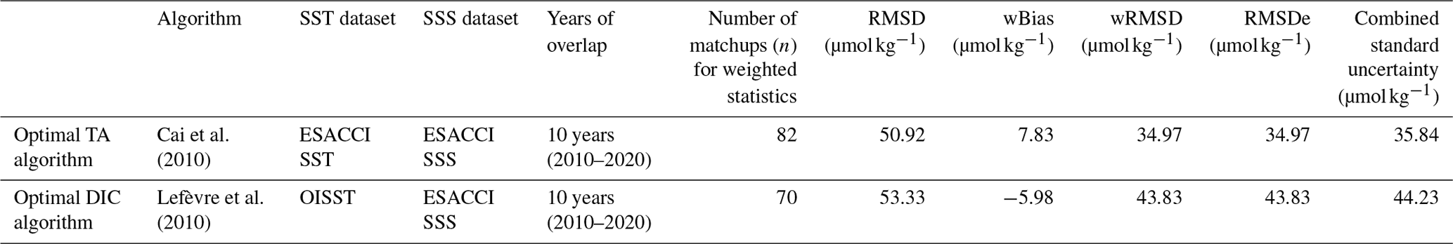
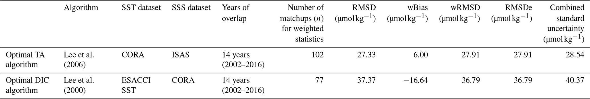
Table 2 Summary table of the best combination of algorithm and SST/SSS datasets (aka the “optimal algorithms”) in the Congo River domain. These optimal algorithms were determined by selecting the algorithm with the lowest RMSDe where there was at least 8 years of data.

3 Results

3.1 Algorithm evaluation

The RMSDe algorithm evaluation results for the Amazon and Congo with respect to the TA and DIC are shown in Fig. 1. From these RMSDe values, we selected the algorithm combination with the lowest RMSDe for both regions as the “optimal algorithms”. The optimal algorithms were then used to produce OceanSODA-UNEXE. In the Amazon, the optimal algorithm to generate the TA data was Cai et al. (2010) with ESACCI SST and ESACCI SSS (Table 1). To generate DIC for the Amazon, the best algorithm was Lefèvre et al. (2010) using OISST SST and ESACCI SSS. In the Congo, the optimal algorithm to generate the TA data was Lee et al. (2006) with CORA SST and ISAS SSS (Table 2). For DIC in the Congo, the optimal algorithm was Lee et al. (2000) with ESACCI SST and CORA SSS.

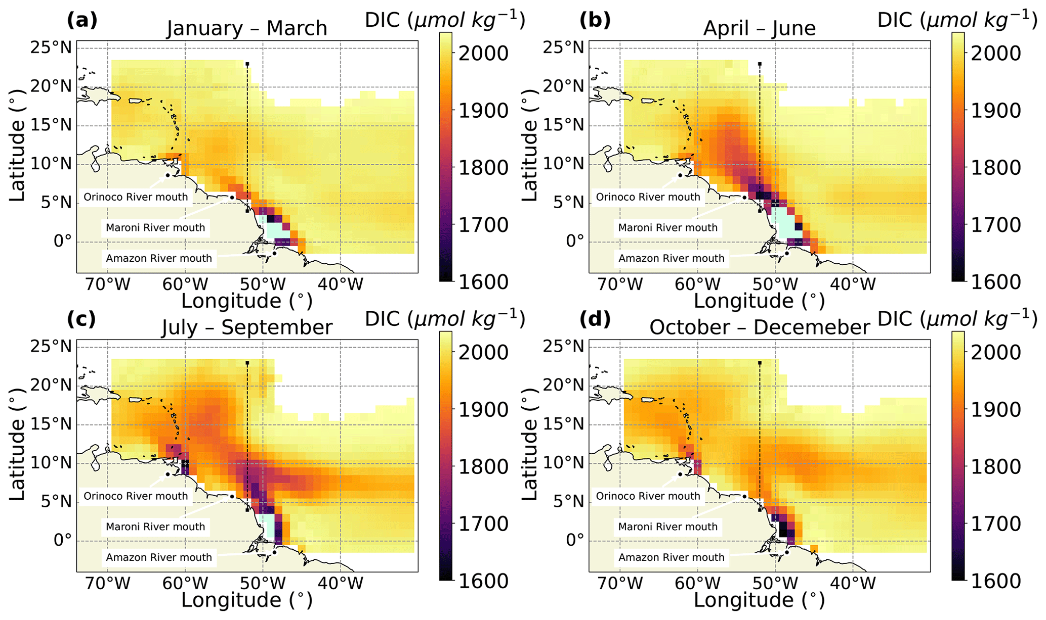
Figure 2 Seasonally averaged DIC for the Amazon plume region in (a) January–March, (b) April–June, (c) July–September and (d) October–December. Land outlines are shown in beige. Ocean regions out of bounds or where there was no algorithm output are left white. Algorithm data below 1600 µmol kg⁻¹ at the river outflows are shown in mint green. The mouths of the Amazon, Orinoco and Maroni rivers are labelled. The 52^∘ W meridional section used for the Hovmöller plot in Fig. 4 is indicated as a black dashed line.

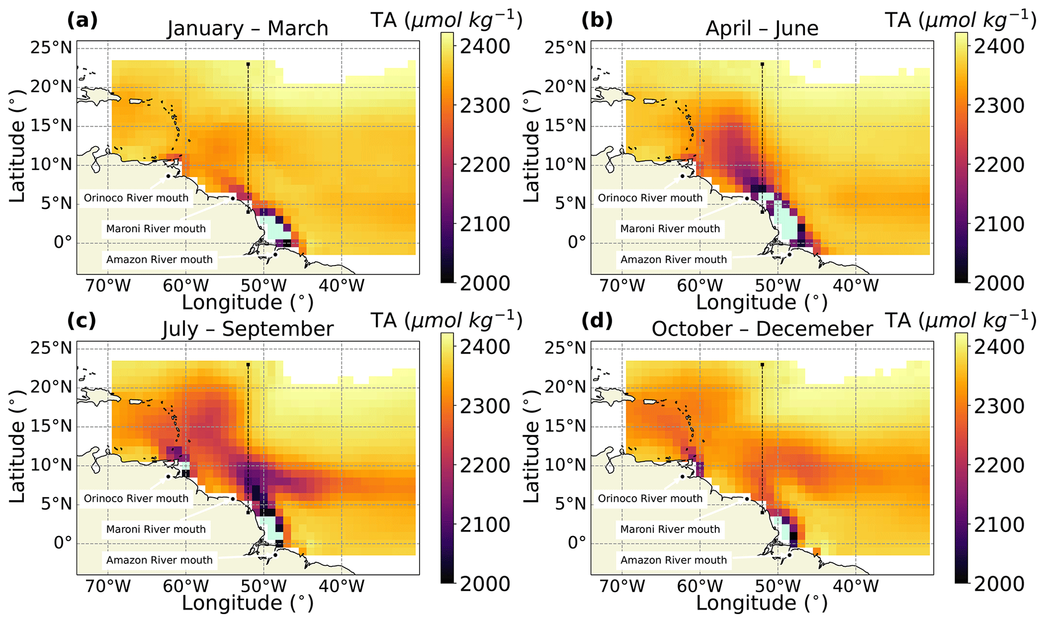
Figure 3 Seasonally averaged TA for the Amazon plume region in (a) January–March, (b) April–June, (c) July–September and (d) October–December. Land outlines are shown in beige. Ocean regions out of bounds or where there was no algorithm output are left white. Algorithm data below 2000 µmol kg⁻¹ at the river outflows are shown in mint green. The Orinoco and Maroni rivers are labelled. The 52^∘ W meridional section used for the Hovmöller plot in Fig. 4 is indicated as a black dashed line.

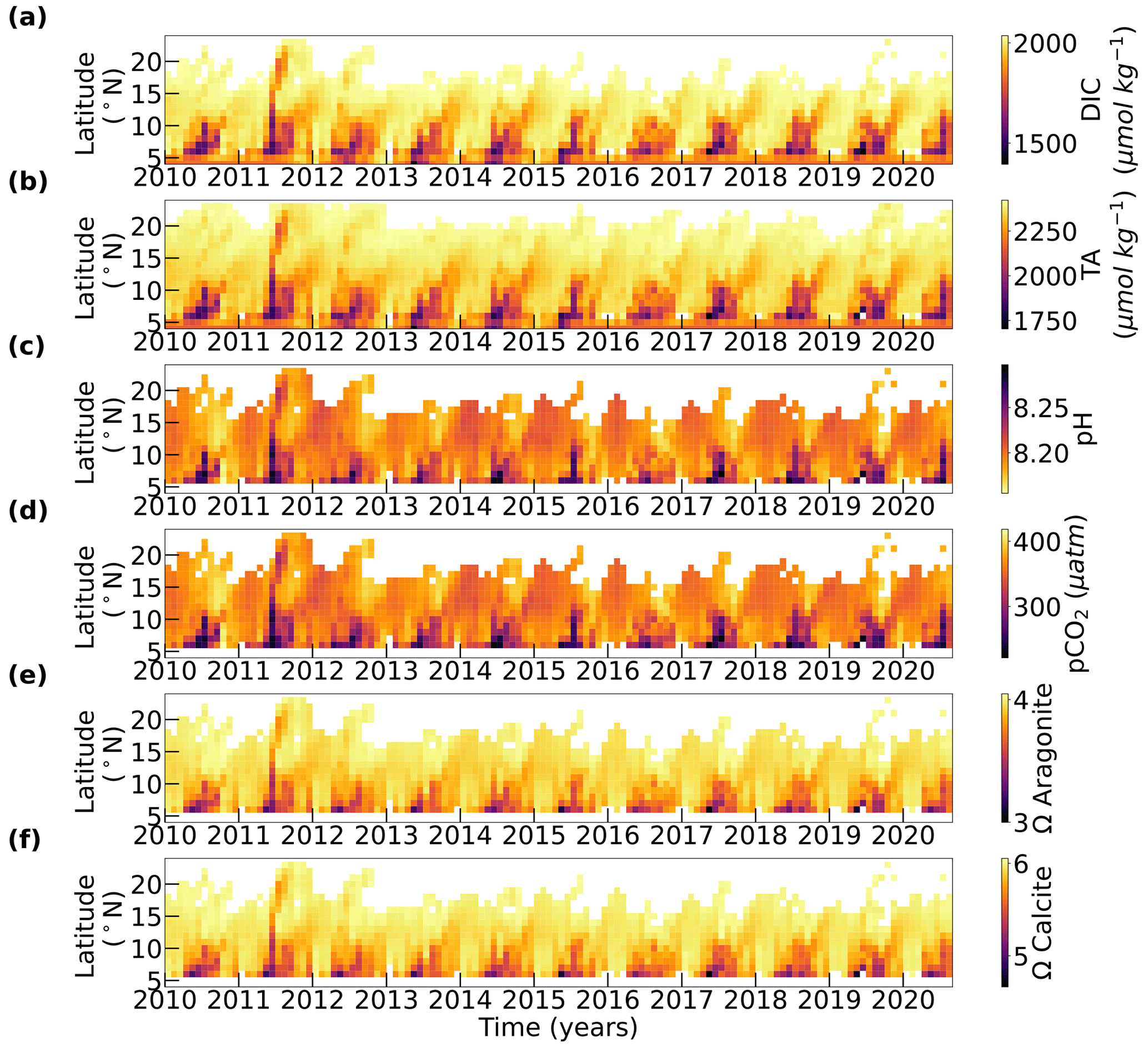
Figure 4 Hovmöller plots of the Amazon outflow region for (a) DIC, (b) TA, (c) pH on the free scale, (d) pCO₂, (e) Ω aragonite and (f) Ω calcite. The plots span the 52^∘ W meridian from 4 to 24^∘ N. The plots cover the temporal overlap period of the TA and DIC datasets (2010–2020).

3.2 Dataset output

3.2.1 Amazon dataset

The primary output datasets are the monthly gridded carbonate system variables (DIC and TA). The seasonal progression of both these variables is shown in the Amazon outflow region in Figs. 2 and 3. There is a large range of DIC and TA in this region, with high values (DIC ∼ 2000 µmol kg⁻¹ and TA ∼ 2350 µmol kg⁻¹) in the open ocean. The lowest values (DIC and TA ∼ 1400 µmol kg⁻¹) are located at the mouth of the river. Intermediate values occur where the plume and ocean water mix. The plume extends to the northwest of the Amazon River mouth (Coles et al., 2013); this is especially visible from April to September (Figs. 2, 3b, 3c), less so from October to March (Figs. 2a, 2d, 3a, 3d), demonstrating the seasonal variability. The region of influence of the Amazon plume extends into the Caribbean between April and June (Figs. 2b, 3b), which is a feature that has been reported elsewhere (Chérubin and Richardson, 2007). From July to September (Figs. 2c, 3c), another large outflow region occurs just off the coast of Venezuela at the mouth of the Orinoco River (Hu et al., 2004). The Orinoco plume is much less prominent in the other seasons. The proximity of the Orinoco River to the Caribbean suggests that the Orinoco plume often reaches the islands between July and September (López et al., 2013). There are some differences between the structure of the average TA and DIC plumes that may indicate active processes in the plume, such as gas exchange, which only affects DIC, or biological production, which affects TA and DIC at different rates. Annual and seasonal data averages over the region shown in Figs. 2 and 3 are provided in Table S3 in the Supplement for DIC, TA, pH, pCO₂, Ω calcite and Ω aragonite.

The temporal aspect of the dataset is presented in Fig. 4 as a meridional Hovmöller plot at 52^∘ W (marked in Figs. 2 and 3) which broadly cuts through the central plume outflow at 4^∘ N, the mixing of the plume up to 10^∘ N and the open-ocean Atlantic water > 10^∘ N. The lowest DIC values (∼ 1400 µmol kg⁻¹) are found in the plume at 4^∘ N, and there is regular seasonality with lower values in October–December and higher values in April–June (Fig. 4a). There does not appear to be much inter-annual variability in the magnitude of the DIC plume in the June–August period, although 2010 and 2013 appear to be weaker (Fig. 4a). The maximum northerly extent of the plume varies from year to year, with higher DIC found at 15^∘ N in the May–August period of 2011. The opposite is true in other years – for example, the plume does not extend as far northwards in 2013 (Fig. 4a). TA shows much more inter-annual variability (Fig. 4b). The minimum plume values do not always occur at the same latitude or at the same time. In most years, the minimum plume values are as low as 1750 µmol kg⁻¹, but this was not the case in 2016. The northward extent of the plume is variable: in some years, the plume extended much further north (e.g. June–July 2011), whereas the plume influence was not as detectable further north in other years (e.g. May–July 2016). The period of time where the plume dominates the region is also variable: in some years the peak plume intensity, which begins in May, lasts through to September, whereas it is already declining in July in other years.

As pCO₂ and pH are derived from DIC and TA, the behaviour of these variables mirrors that of TA and DIC (Fig. 4c, d). The river plume always has above-neutral pH and occasionally extends far to the north (e.g. June–July 2011). There are low pCO₂ values (< 200 µatm) in the plume that are much lower than some of the other values observed in the plume (Lefèvre et al., 2017). Calcite and aragonite saturation states have the expected magnitude in open-ocean regions and are lower in the plume, with Ω calcite levels ∼ 3 in the plume.

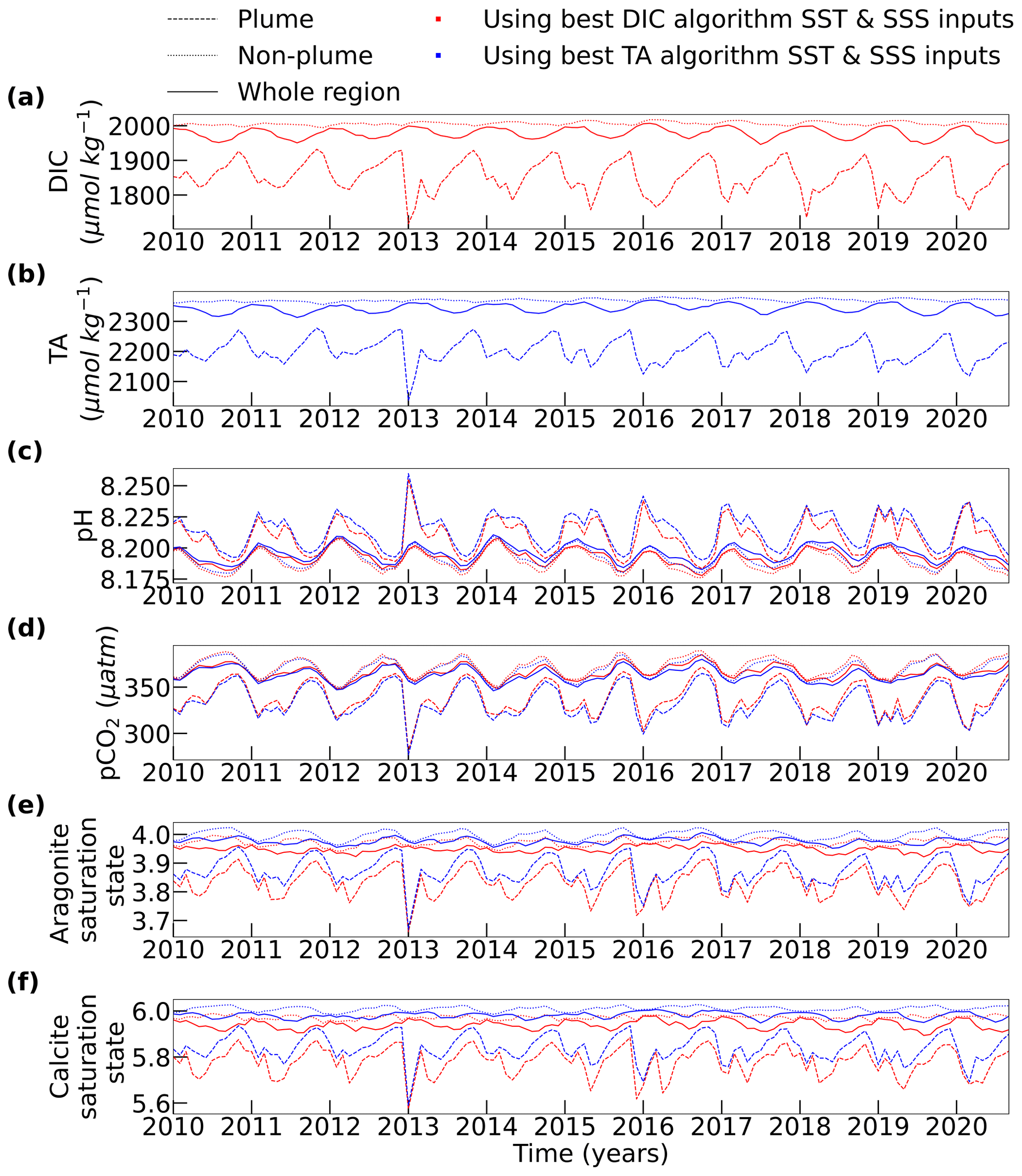
Figure 5 Time series of spatially averaged (a) DIC, (b) TA, (c) pH, (d) pCO₂, (e) Ω aragonite and (f) Ω calcite in the Amazon region. The plots spans the temporal overlap period of the TA and DIC datasets (2010–2020). Data are averaged across the whole region (solid line) as well as in the plume defined as S < 35 (dashed line) and outside of the plume S > 35 (dotted line). The line colour corresponds to variables that were calculated with the SST and SSS datasets selected during the DIC algorithm evaluation (red) and the TA algorithm evaluation (blue).

The gridded data can also be spatially averaged to show the evolution of each of the carbonate system variables in time within the plume (defined as SSS < 35; Grodsky et al., 2014), outside the plume (SSS > 35) and over the whole region (Fig. 5). The mean DIC calculated across whole region shows a very consistent seasonal pattern, with higher DIC in December–February (∼ 2000 µmol kg⁻¹) and lower DIC in June–August (∼ 1970 µmol kg⁻¹). The mean values within the plume are much lower; the lowest DIC values (∼ 1700 µmol kg⁻¹) are seen in December–February and the highest values (∼ 1900 µmol kg⁻¹) are during September–October. The mean non-plume values show much smaller seasonal variability. In the plume, outside of the plume and over the whole region, surface DIC is very similar from year to year. The mean DIC within the plume reaches a minimum in 2013 that is much lower than all other years. Non-plume DIC values increase by 0.49 $\mathrm{\mu }\mathrm{mol}{\mathrm{kg}}^{-\mathrm{1}}{\mathrm{yr}}^{-\mathrm{1}}$. TA across the whole region is inter-annually consistent, with a seasonal maximum in December–February (∼ 2360 µmol kg⁻¹) and minimum in July–August (∼ 2330 µmol kg⁻¹), whereas TA within the plume shows a seasonal maximum in October (∼ 2250 µmol kg⁻¹) and a minimum in April–May (∼ 2150 µmol kg⁻¹). The annual minimum within the plume varies from December to March, while the maximum consistently occurs in October and November; there is also considerable inter-annual variability in the timing of the annual minimum, with much lower TA in the December–February periods of 2012–2013 and 2017–2018 than over the same period in other years. Non-plume TA values increased by 0.76 $\mathrm{\mu }\mathrm{mol}{\mathrm{kg}}^{-\mathrm{1}}{\mathrm{yr}}^{-\mathrm{1}}$. It should be noted that the whole region is out of phase with the plume; this is because, whilst the plume is more dilute, this effect is outweighed by the larger plume between May and August.

For pH, there is a weak seasonal trend outside the plume. In contrast there is a lot more variability in the plume, with the highest pH values (∼ 8.225) occurring in December and the lowest values (∼ 8.2) in September. The best SST and SSS datasets from the DIC algorithm predict that the pH will be > 0.1 higher than the best SST and SSS datasets from the TA algorithm between January and March. The two estimates agree within < 0.1 pH units for the other 9 months of the year. For pCO₂, also computed from TA and DIC, mean values in the non-plume region and over the whole region were very stable, which is consistent with the minimal season variability seen in oligotrophic oceans. Whereas there was considerable variability in plume pCO₂, with average values of ∼ 325 µatm seen in the plume in March and values of ∼ 350 µatm in August, the differences between the pCO₂ calculated with the different SST and SSS datasets was very small, with differences < 5 µatm most of the year. The average calcite and aragonite saturation states are in the typical range for seawater and are much greater than the critical thermodynamic threshold for calcification with a value of one (Waldbusser et al., 2016). It should be noted that an aragonite saturation state threshold of three has also been recommended for warm-water corals (Guinotte et al., 2003), and other studies have since shown that warm-water corals can still adapt and survive in these conditions (Enochs et al., 2020; Uthicke et al., 2014). There are periods in the data, such as at the start of 2019, in which the aragonite saturation state falls below three. The mean saturation states within the plume are lower than those found in the wider region.

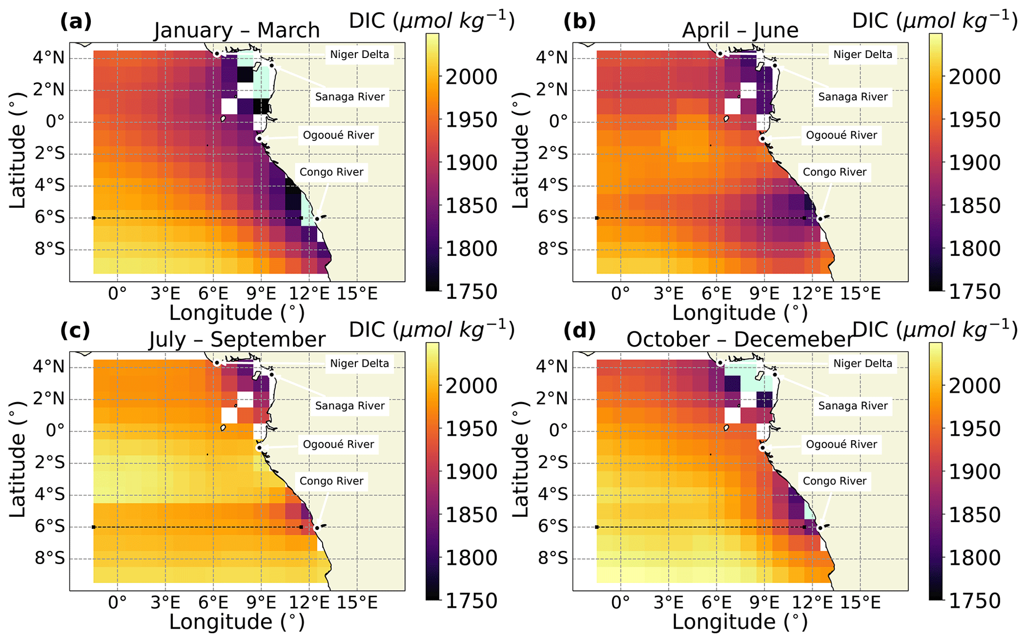
Figure 6 Seasonally averaged DIC for the Congo outflow region in (a) January–March, (b) April–June, (c) July–September and (d) October–December. Land outlines are shown in beige. Ocean regions out of bounds or where there was no algorithm output are left white. Algorithm data below 1750 µmol kg⁻¹ at the river outflows are shown in mint green. The Niger River delta and the mouths of the Congo, Ogooué and Sanaga rivers are labelled. The 6^∘ S meridional section used for the Hovmöller plot in Fig. 8 is indicated a bold dashed line.

3.2.2 Congo dataset

In the Congo outflow region, there is a strong seasonal variation in DIC (Fig. 6). From July to September (Fig. 6c), there are two regions of low DIC: one directly at the outflow point of the Congo River and another at the outflow point of the Niger River delta. The outflows of both of these river-dominated regions extend directly west, aligned with the South Equatorial Current in the eastern Atlantic (Hopkins et al., 2013). In October–December (Fig. 6d), the spatial influence of the Congo outflow is smaller, possibly due to water masses moving northwards along the coast. Into January–March (Fig. 6a), there is a region of low DIC along the whole coast, representing the intensification of the Niger and Congo discharges at this time of year (Chao et al., 2015). In April–June (Fig. 6b), the coastal water mass separates, becoming two distinct outflows, and the outflows reach their greatest westward extent, covering almost the whole domain.

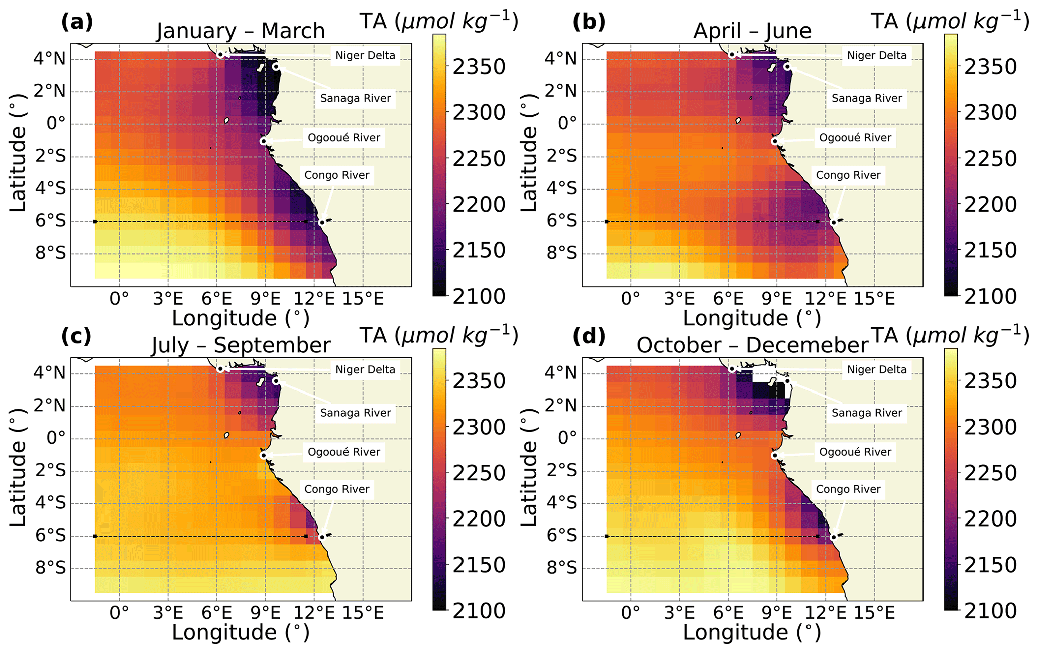
Figure 7 Seasonally averaged TA for the Congo outflow region in (a) January–March, (b) April–June, (c) July–September and (d) October–December. Land outlines are shown in beige. Ocean regions out of bounds or where there was no algorithm output are left white. The Niger River delta and the mouths of the Congo, Ogooué and Sanaga rivers are labelled. The 6^∘ S meridional section used for the Hovmöller plot in Fig. 8 is indicated a bold dashed line.

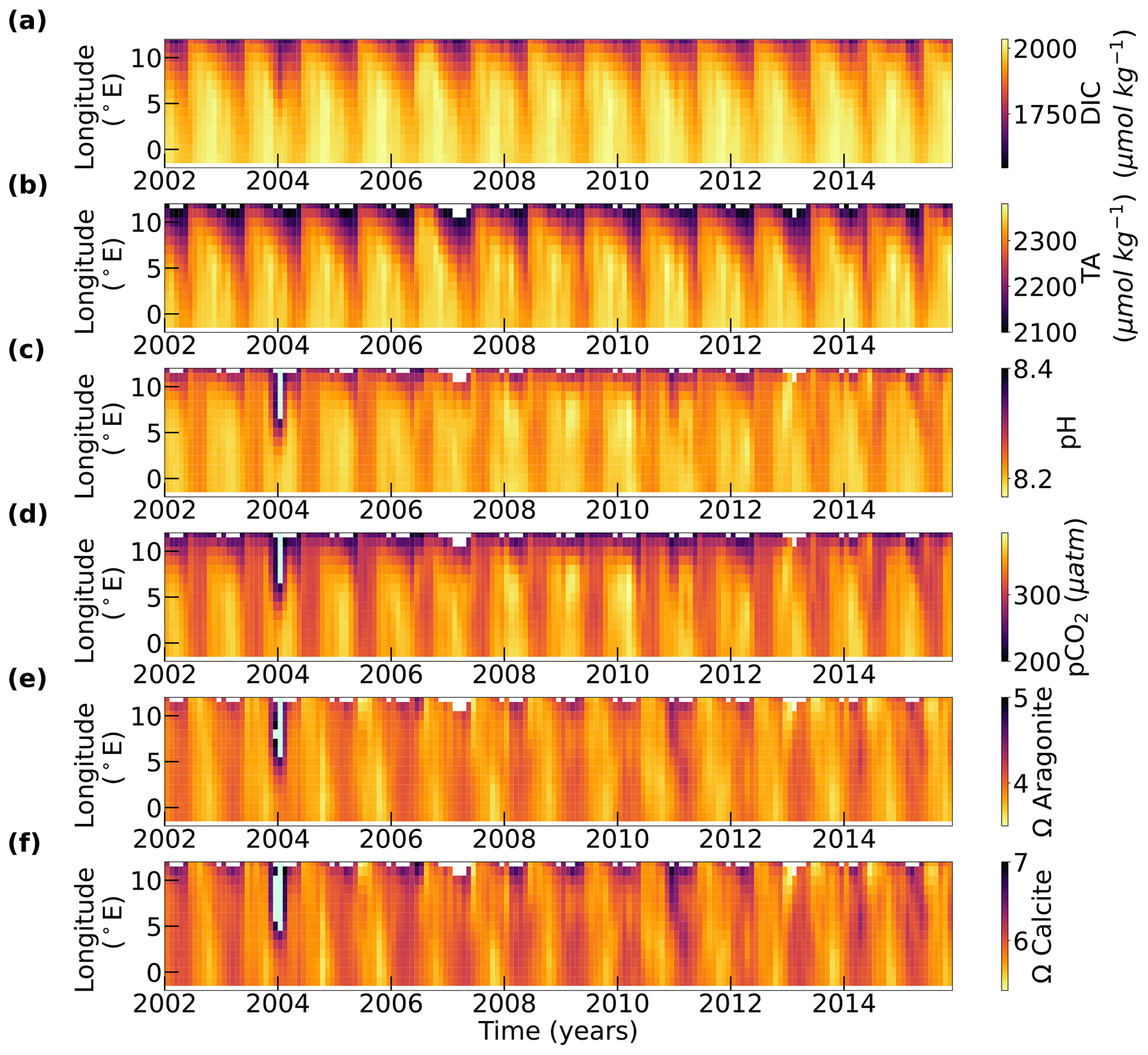
Figure 8 Hovmöller plots of (a) DIC, (b) TA, (c) pH, (d) pCO₂, (e) Ω aragonite and (f) Ω calcite for the Congo outflow region. The plots are centred on the 6^∘ S slice that spans from 2^∘ W to 12^∘ E. Values of pH > 8.4, pCO₂ < 200 µatm, Ω calcite > 5 and Ω calcite > 7 in the river outflow in December 2003 are shown in mint green. The plots spans the temporal overlap period of the TA and DIC datasets (2002–2016), and thus the period for which the rest of the carbonate system was generated.

Similar trends are seen in TA (Fig. 7), with two distinct outflow regions in July to September (Fig. 7c). The outflows begin to intensify in October–December (Fig. 7d). The lowest TA values are observed to the east of the Niger River delta outflow in January–March (Fig. 7a). Unlike in Fig. 6a, the outflows remain distinct in Fig. 7a. Between April and June, the outflow reaches its maximum spatial extent as it flows out to the west where it is has a detectable impact across the region.

A zonal section at 6^∘ S was used to construct a Hovmöller plot of variables in the Congo (Fig. 8). This latitude is centred across the outflow of the Congo River. In contrast to the Amazon, much of the plot region is masked in between May and July, as the published algorithms were not valid for the full range of environmental conditions experienced by the region.

The DIC plot (Fig. 8a) shows that the outflow is low in DIC (∼ 1800 µmol kg⁻¹) and that the open ocean is higher (∼ 2050 µmol kg⁻¹). The highest values are found in the January–March period, consistent with Fig. 6a. The outflow is detectable over the widest area in the March–June period in all years. Whilst there is one period of intense outflow each year, there is also some indication that a weaker outflow is intermittently detectable in the data (shown as vertical streaks in Fig. 8a). TA (Fig. 8b) shows an almost identical pattern to DIC. The lowest TA values (∼ 2100 µmol kg⁻¹) were observed between January and March, and slightly higher values (∼ 2200 µmol kg⁻¹) were seen when the outflow extended further west between April and June.

Higher pH values (∼ 8.3) were observed in the outflow compared with the open ocean (∼ 8.2) (Fig. 8c). Previous studies have measured low pH values in the main body of the river and its tributaries (Wang et al., 2013; Bouillon et al., 2014), the higher pH values at the mouth of the river may be due to complex carbonate speciation. The minimum pCO₂ values are very low (∼ 200 µatm) in the inner part of the outflow (Fig. 8d), whereas values in the outer part of the outflow are closer to the expected pCO₂ values of around 350 µatm. (da Cunha and Buitenhuis, 2013). Mirroring the trends in pH, the calcite and aragonite saturation states (Fig. 8e, f) are higher in the outflow relative to the open ocean. Anomalous pH, pCO₂, and calcite and aragonite saturation state values in December 2003 are likely associated with heavy rainfall over southern Central Africa (Kadomura, 2005).

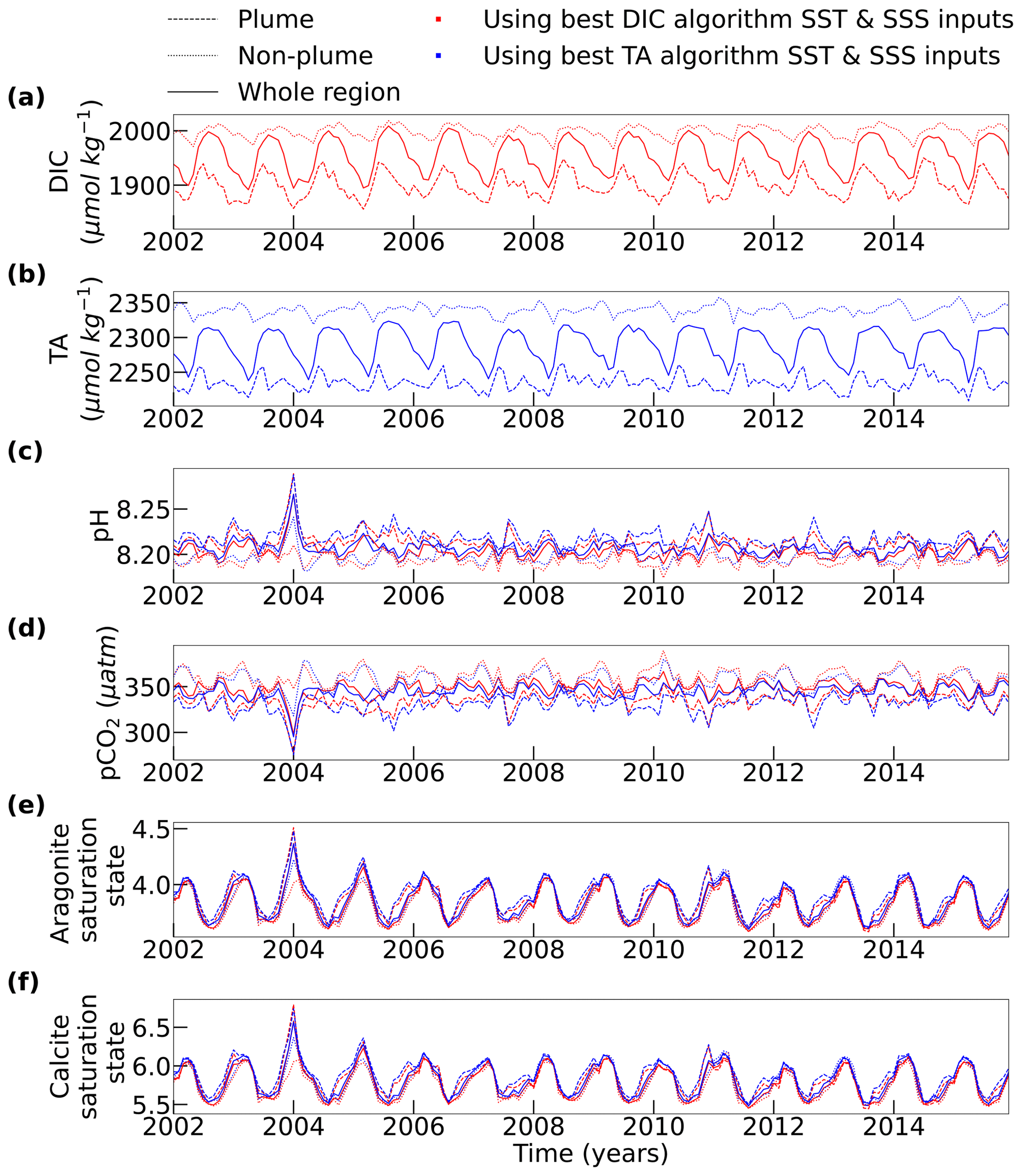
Figure 9 Time series of spatially averaged (a) DIC, (b) TA, (c) pH, (d) pCO₂, (e) Ω aragonite and (f) Ω calcite in the Congo region. The plots spans the temporal overlap period of the TA and DIC datasets (2002–2016). Data are averaged across the whole region (solid line) as well as in the outflow defined as S < 35 (dashed line) and outside of the outflow S > 35 (dotted line). The line colour corresponds to variables that were calculated with the SST and SSS datasets selected during the DIC algorithm evaluation (red) and the TA algorithm evaluation (blue).

The mean DIC and TA across the whole Congo region, in the outflow and out of the outflow are very consistent from year to year (Fig. 9a, b). The yearly TA and DIC minima occur at approximately the same time and are the same magnitude most years. DIC and TA values are always higher in the non-outflow region than in the outflow. This consistency is also seen in the propagated variables, pH (Fig. 9c), pCO₂ (Fig. 9d), and the aragonite and calcite saturation states (Fig. 9e, f), all of which show very minor differences between the outflow and non-outflow regions.

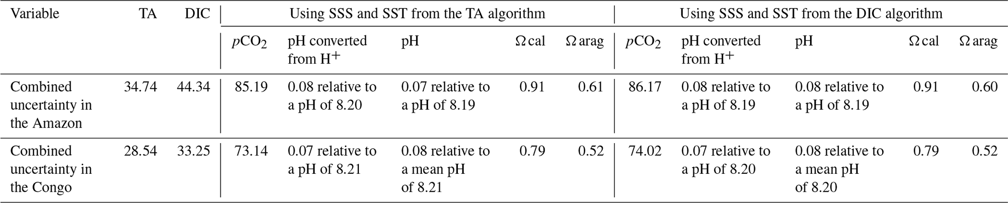
Table 3 Output variable uncertainties in the two regions of OceanSODA-UNEXE. TA and DIC uncertainties are the combined standard uncertainties from the algorithm evaluation. The uncertainty for the remaining carbonate system variables are the average of the spatially varying propagated uncertainties for each of those variables calculated with the SST and SSS pair from either the TA or DIC algorithm. Note that, due to the logarithmic nature of pH, uncertainty is calculated as 1σ in pH units and also in pH units, where variability was determined in H⁺ as $-{\text{log}}_{\mathrm{10}}\left(\stackrel{\mathrm{‾}}{{\mathrm{H}}^{+}}\right)+{\text{log}}_{\mathrm{10}}(\stackrel{\mathrm{‾}}{{\mathrm{H}}^{+}}+\mathrm{1}\mathit{\sigma }{\mathrm{H}}^{+})$.

3.3 Uncertainty assessment

The TA and DIC combined standard uncertainties from the algorithm evaluation are shown in Tables 1 and 2. The combined standard uncertainties for the optimal algorithms used to generate the time series dataset are reproduced in Table 3. The combined standard uncertainties are the first Type-A uncertainty evaluation, which can be thought of as a top-down estimate. The spatially averaged uncertainties of the remaining carbonate system variables using this top-down estimate are shown in both outflow regions (Table 3). The uncertainties of the remaining carbonate system variables appear to be weakly dependent on the choice of the SST and SSS datasets used to calculate them in PyCO2SYS (Table 3). Uncertainties are provided as absolute values, rather than as percentages, because of the steep gradient in values across the plume; however, if required, the uncertainty values can be expressed as a percentage using the minimum, maximum and mean values from Table S4 in the Supplement.

The second Type-A uncertainty evaluation (using the algorithm RMSD from the literature and the uncertainties in the inputs) can be thought of as a bottom-up estimate. For this bottom-up estimate, the average combined standard uncertainties in TA and DIC are 8.52 and 16.59 in the Amazon and 17.23 and 14.25 in the Congo, respectively. These values are much lower than those from the top-down uncertainty evaluation, as this uncertainty evaluation does not fully account for spatial and depth variability. RMSD values from the literature do not fully capture all the measurement variability in the bottom-up uncertainty evaluation. The bottom-up evaluation does account for uncertainty in the input SST and SSS datasets, suggesting that spatial and depth variabilities and differences between the in situ data (used to evaluate the uncertainties) are likely dominating the uncertainty budget.

Table 4 In situ measurement variabilities for TA, DIC, pH and pCO₂ are calculated as the standard deviation of the reference output (MDB). For the Amazon, ESACCI SST and ESACCI SSS were the combination used with the MDB, whereas CORA SST and ISAS SSS were used for the Congo. Note that, due to the logarithmic nature of pH, uncertainty is calculated as 1σ in pH units and also in pH units, where variability was determined in H⁺ as $-{\text{log}}_{\mathrm{10}}\left(\stackrel{\mathrm{‾}}{{\mathrm{H}}^{+}}\right)+{\text{log}}_{\mathrm{10}}(\stackrel{\mathrm{‾}}{{\mathrm{H}}^{+}}+\mathrm{1}\mathit{\sigma }{\mathrm{H}}^{+})$.

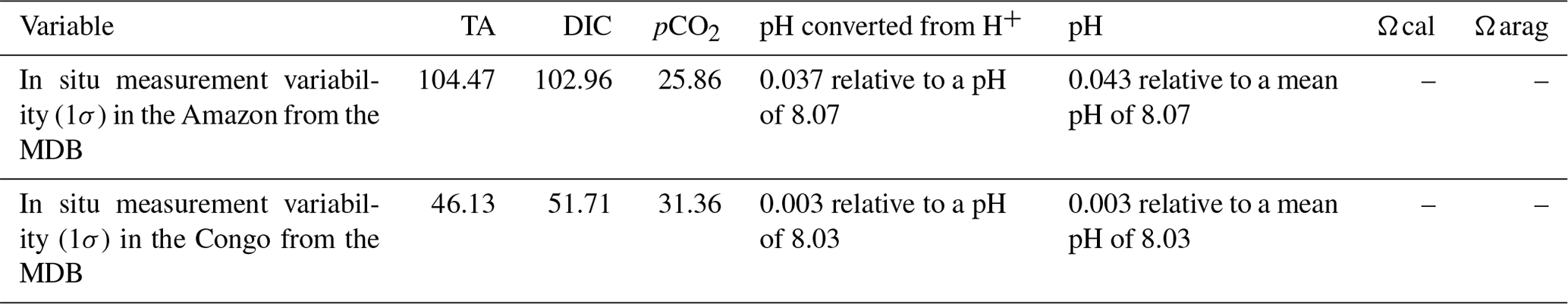
As the top-down uncertainty evaluation is more robust, it is the preferred uncertainty estimate. By comparing the uncertainties with the natural variability in TA and DIC (Table 4), it is clear that the dataset uncertainty is less than the natural variability in data in both riverine regions. Although the propagated uncertainties for pCO₂ and pH are larger than the natural variability, this is only because the pCO₂ and pH data generated in OceanSODA-UNEXE have full spatiotemporal coverage, including in the high-variability plume, compared with the pCO₂ and pH in situ data in the MDB.

4 Discussion

The algorithm evaluation (Fig. 1) demonstrated that the choice of input SSS dataset to the TA and DIC algorithms makes the biggest difference in reducing the RMSDe in TA and DIC. SST tends to be a secondary term in the majority of the algorithms and, therefore, has less of a controlling effect. The choice of the literature TA or DIC algorithm itself impacts RMSDe to a much smaller extent than the choice of input SSS datasets. The prominence of SSS terms in the majority of the algorithms explains why the RMSDe is much more sensitive to the choice of SSS dataset compared with SST dataset, as SST is a secondary term in the majority of the algorithms. Whilst some algorithms did perform better than others, the differences were so slight that it may not be that helpful to declare which of the algorithms are the best outright, especially as this could change in the future with more data.

The requirement of having n = 30 matchups to calculate the weighted statistics has a large impact on the choice of optimal algorithms. By including this stipulation, some of the more recent salinity input datasets are effectively deselected because there are not enough contemporary measurements over their temporal range to allow their evaluation, particularly in the Congo region. For example, the SMAP satellite was only launched in 2015, and there were not enough in situ matchups in either region to be able to fully assess the RSS-SMAP dataset. Therefore, using ISAS for salinity in the optimal TA algorithm in the Congo (where data are available from 2002 onwards) increases the number of matchups by a factor of 20 compared with using RSS-SMAP (Table 2). Given time, the number of matchups with the satellite-only products will increase, allowing them to be fully evaluated. Considering the better spatial coverage of the satellite-only products, it is likely that, in the near future, the best algorithm combinations to generate updates to this product will all use satellite-derived SSS and SST. The recent proliferation of certified reference materials when measuring TA (Dickson et al., 2003) and DIC (Dickson, 2001) should also mean that newer in situ data will have lower uncertainties. The relatively low number of in situ data limits the potential use of neural-network-based approaches to estimate the carbonate system in these outflows, and significantly more in situ data would be needed (for training and testing) before these approaches could likely be applied.

By comparing the two Type-A uncertainty estimates, the standard combined uncertainty estimate (accounting for measurement uncertainty, spatial uncertainty, depth uncertainty and algorithm uncertainty – aka top down) and the second Type-A uncertainty evaluation (propagated input uncertainties through the literature algorithm – aka bottom up), the contribution of different factors to the uncertainty can be dissected. The bottom-up uncertainty estimates are much smaller than the top-down uncertainty estimates, reflecting the fact that less of the uncertainty has been considered in the bottom-up uncertainty estimates. The difference between the top-down and bottom-up estimates can be mainly attributed to the spatial and depth uncertainty, which is accounted for by using the MDB in the algorithm evaluation. Land et al. (2019) noted that reducing the uncertainty of the in situ measurements was just as important as all of the remaining uncertainties in their full methodology. Further reducing the standard combined uncertainty is challenging and would require either improvements in satellite SSS retrievals (Vinogradova et al., 2019) or improvements in how uncertainty is quantified in the GLODAP data (a huge challenge give the different systems and protocols used by different laboratories) (Bockmon and Dickson, 2015).

The time series data demonstrate that there is low TA and DIC in the river outflows of both regions. The time series data clearly show that the discharge of the outflows and their zone of influence changes seasonally. Our results are consistent with previous observations that the Amazon plume extent is smallest between January and March (Fournier et al., 2015) and largest between April and June, when it expels low-TA and low-DIC waters (Cooley and Yager, 2006). The Amazon plume reaches the Caribbean, as previously shown by Hellweger and Gordon (2002). The time series data identify that saturation states can drop below three in parts of the Amazon plume (Table S4), which has implications for ocean acidification research, especially for researchers studying coral reefs. The non-plume DIC and TA trends of 0.49 and 0.76 $\mathrm{\mu }\mathrm{mol}{\mathrm{kg}}^{-\mathrm{1}}{\mathrm{yr}}^{-\mathrm{1}}$ are consistent with the decadal increases in salinity-normalized DIC (4.54 µmol kg⁻¹) and salinity-normalized TA (7.39 µmol kg⁻¹) in the 2010s from the Bermuda Atlantic Time-series Study site (Bates and Johnson, 2020). The results identify that the discharge of the Congo outflow is greatest between January and March and veers towards West Africa, which is consistent with work by Hopkins et al. (2013).

The time series data comprise over 10 years of carbonate system data for two of the world's largest rivers by discharge. One immediate use for the time series data would be the assessment of the inorganic carbon flow of both of these rivers over time. The time series data could also be used to investigate the impact of charges in land use within the river basin, e.g. deforestation impacts on river discharge and inorganic carbon flow into rivers (Bass et al., 2014). If the impact of land use changes were identifiable within the data, these approaches may prove to be a useful tool for monitoring the effectiveness of policy or management actions addressing climate change and biodiversity loss in the Amazon Basin. The time series data could also be used for ocean acidification research (Land et al., 2015), as these rivers discharge enough fresh water to influence carbonate saturation states. The tropical reefs of the Caribbean are infrequently impacted by the Amazon plume (Chérubin and Richardson, 2007); the impact of the low-pH waters on reef health is of great concern (Hoegh-Guldberg et al., 2007) and could be explored with the time series data. Ocean acidification has been shown to impact foraging behaviour in fish (Jiahuan et al., 2018) and sharks (Rosa et al., 2017); thus, the time series data could be used in conjunction with GPS tracks of fish or marine mammals to see if the outflows alter foraging behaviour. The time series data could also be used to explore CO₂ fluxes in the Amazon outflow, building upon more recent estimates (Olivier et al., 2022; Ibánhez et al., 2016; Mu et al., 2021).

5 Data availability

The dataset described in this paper is freely available at PANGAEA (https://doi.org/10.1594/PANGAEA.946888, Sims et al., 2023). The OceanSODA-MDB data are available at https://doi.org/10.12770/0dc16d62-05f6-4bbe-9dc4-6d47825a5931 (Land and Piollé, 2022). All of the remote sensing datasets needed to create the gridded products are freely available from their respective online repositories.

6 Code availability

The code used to run this analysis and download the remote sensing datasets is provided in the Supplement and is freely available at GitHub (https://github.com/Richard-Sims/Sims_2023_OceanSODA-UNEXE, last access: 25 April 2023) and on Zenodo (https://doi.org/10.5281/zenodo.7863884, Sims and Holding, 2023). The code can be run on a desktop computer and requires no specialist computing facilities. For example, a laptop with an Intel i7-4800MQ 2.70 GHz CPU and 8 GB of memory can complete the algorithm evaluation in around 1 h. On the same machine, the remote sensing datasets take several days to download and reprocess; this is partially subject to local internet speeds and host server speeds. Creating the gridded datasets for each region takes 2 h on the same machine.

7 Conclusions

OceanSODA-UNEXE is a time series dataset of the carbonate system in the outflow regions of the Amazon and Congo rivers. Optimal TA and DIC data are generated with the optimal combination of published algorithms and input datasets, which is determined by an exhaustive round-robin inter-comparison evaluation. By using a specially designed matchup database for the algorithm evaluation, uncertainties due to spatial and depth variability in the in situ references have been minimized. TA, DIC, SST and SSS are used as inputs into PyCO2SYS to calculate the remaining carbonate system variables (pH and pCO₂). TA and DIC are provided with standard combined uncertainties from a Type-A uncertainty evaluation, whereas pH and pCO₂ are provided with propagated uncertainties from PyCO2SYS. The assessed uncertainties are lower than the natural variability within these regions, and the main features of both river outflows are evident in all of the carbonate system variable outputs. Potential uses for these data could include evaluating the riverine carbon flux from the land into the ocean resulting from the Amazon and Congo rivers or evaluating the extent that river-driven episodic changes in the carbonate system may be having on sensitive coral reefs that interact with the outflows.