Updated observations of clouds by MODIS for global model assessment

This paper describes a new global dataset of cloud properties observed by MODIS relying on the current (collection 6.1) processing of MODIS data and produced to facilitate comparison with results from the MODIS observational proxy used in climate models. The dataset merges observations from the two MODIS instruments into a single netCDF file. Statistics (mean, standard deviation, and number of observations) are accumulated over daily and monthly timescales on an equal-angle grid for viewing and illumination geometry, cloud detection, cloud-top pressure, and cloud properties (optical thickness, effective particle size, and water path) partitioned by thermodynamic phase and an assessment as to whether the underlying observations come from fully or partly cloudy pixels. Similarly partitioned joint histograms are available for (1) optical thickness and cloud-top pressure, (2) optical thickness and particle size, and (3) cloud water path and particle size. Differences with standard data products, caveats for data use, and guidelines for comparison to the MODIS simulator are described. Data are available on daily (https://doi.org/10.5067/MODIS/MCD06COSP_D3_MODIS.062; NASA, 2022b) and monthly (https://doi.org/10.5067/MODIS/MCD06COSP_M3_MODIS.062; NASA, 2022a) timescales.

1 MODIS observations of clouds and the assessment of global models

The distribution of cloud radiative properties strongly impacts Earth's energy balance (e.g., Hartmann et al., 1992). Uncertainty in how clouds will respond to anthropogenic forcing is responsible for most of the difficulty in estimating climate sensitivity (Sherwood et al., 2020), largely because clouds are so tightly coupled to atmospheric circulations (Bony et al., 2015) across a wide range of scales. Clouds' impacts on the global and local energy budgets, and on the distribution of precipitation, motivate efforts to assess the distribution of clouds produced by global models against observations (e.g., Pincus et al., 2012; Klein et al., 2013).

Observations from space offer the most globally uniform observations of clouds, but direct comparisons with predictions from numerical models are complicated by differing definitions of cloudiness, sampling errors introduced by the observing system, and differing scales in the observations compared to the models. The ISCCP simulator (Yu et al., 1996; Klein and Jakob, 1999; Webb et al., 2001) was introduced several decades ago to allow for more informative comparisons. The ISCCP (International Satellite Cloud Climatology Project) proxy is diagnostic software that runs within a climate model and roughly maps the clouds as represented by the model to synthetic observations as would be obtained from the ISCCP program (Rossow and Schiffer, 1991). Insights from the ISCCP simulator inspired a range of other such proxies focused on clouds, many of which have been packaged together in the CFMIP Observation Simulator Package (COSP, where CFMIP is the Cloud Feedback Model Intercomparison Project; see Bodas-Salcedo et al., 2011; Swales et al., 2018).

Among other simulators, COSP includes a proxy for MODIS observations of clouds, as described in Pincus et al. (2012). Compared to ISCCP and other passive sensors, MODIS, described more fully below, offers a better characterization of cloud thermodynamic phase and routine estimates of cloud particle size. Synthetic observations from the MODIS simulator, namely joint probability distributions of cloud optical thickness and particle size, are requested as part of phase 3 of the Cloud Feedback Model Intercomparison Project (Webb et al., 2017). Output is requested only for the daylit portion of the globe, where richer information is available from passive sensors.

Because the MODIS proxy is most widely used alongside other proxies within COSP, the output is normally configured to complement the other proxies in the suite. A number of barriers arise in comparing this focused subset of data with the standard observational datasets produced by the MODIS Science Team (e.g., King et al., 2013). These range from mundane but important hurdles, such as the files being in different formats, and different histogram discretizations to more fundamental issues, such as data produced in the simulator having no direct counterpart in the observational data. Pincus et al. (2012) described an initial dataset designed to lower those barriers. That dataset, produced with an earlier version of the underlying MODIS data, post-processed standard monthly data files and invoked a number of assumptions to make the observations more compatible with fields produced by the simulator. The system was fragile and ceased production when NASA updated the production of MODIS datasets. Observations up to September 2016 remain available at https://ladsweb.modaps.eosdis.nasa.gov/archive/NetCDF/L3_Monthly/V02/ (last access: 15 July 2022). These data are currently offline but will be available again at the end of summer 2023.

Here we describe a new global dataset of cloud properties observed by MODIS, relying on the current processing of MODIS data, and produced to facilitate more convenient comparison with results from the MODIS simulator. The new data, designated MCD06COSP, directly combines MODIS pixel-scale observations of cloud occurrence, cloud-top pressure, and cloud optical properties from Terra (MOD06_L2) and Aqua (MYD06_L2) on daily and monthly timescales. The dataset, produced using a system designed to be more robust to changes in the MODIS pixel-scale data stream, provides a set of custom cloud-related parameters using specific dataset definitions more closely aligned with the MODIS simulator than are the standard datasets. Data are provided in the Network Common Data Format Version 4 (netCDF4) format that is widely used to distribute climate model data.

This paper documents the MODIS COSP Level-3 dataset, with an emphasis on helping users interpret the observations and making informed comparisons to results from the MODIS simulator. This document summarizes and expands upon a longer and more complete users' guide available at https://atmosphere-imager.gsfc.nasa.gov/products/monthly_cosp/documentation (last access: 26 May 2023).

2 How data are produced

MODIS, the Moderate Resolution Imaging Spectroradiometer (Salomonson et al., 1989), is a 36-channel narrowband imaging instrument developed for NASA's Earth Observing System. Two MODIS instruments were launched near the beginning of the 21st century and continue to provide data at the time of writing. NASA's MODIS science team produces a wide range of observational datasets based on measurements from the sensor, including the cloud-related observations described below.

The discussion that follows adopts the MODIS project's terminology to describe in detail how the data are produced. In this terminology, observations at the native resolution (nominally 250 m to 1 km for the MODIS instrument) are referred to as pixels, which are acquired and processed in 5 min granules corresponding to 2030 1 km pixels along the satellite track by 1354 pixels cross-track (nominally 2330 km because pixels sizes increase with scan angle). Each version of the software used in the data processing stream is referred to as a collection. At the time of writing, data are produced using Collection 6.1, as documented in Baum et al. (2012) and Platnick et al. (2017). Data are produced at three distinct levels. Level 1 refers to calibrated geolocated radiances (near-raw data). Level 2 describes retrievals (inferences) of geophysical and/or optical quantities at the pixel scale. Level 3 means observations aggregated in space and time, including the dataset described here.

2.1 Identifying clouds and determining their properties

Here we briefly describe how Level-2 data are produced with the intent of orienting users to the data being provided. For further details on the production of pixel-scale observations, see Platnick et al. (2017), Baum et al. (2012), and Pincus et al. (2012), as well as the references therein.

Pixel-scale (Level-2) estimates of cloud properties are determined in two steps, where the first determines the likelihood that a given pixel contains clouds, and the second estimates cloud properties for cloudy pixels. (A separate processing step determines aerosol properties in the non-cloudy pixels.) Cloud detection relies on a decision tree involving multiple channels and produces a cloud mask at 1 km nominal resolution. The decision trees use different information, depending on whether the pixel is sunlit (daytime) or not, using the criterion that the solar zenith angle is less than 85^∘. Each pixel is flagged according to whether the cloud mask has been determined; determined pixels are flagged with one of four values (confidently cloudy, probably cloud, probably clear, or confidently clear). Cloud fraction at 5 km nominal scale is determined as the ratio of confidently and probably cloudy pixels to all determined pixels. Cloud-top pressure p_c is determined at 5 km scale when at least four of the 25 1 km sub-pixels are cloudy (i.e., when 5 km cloud fraction equals or exceeds 16 %). Cloud-top pressure is estimated using CO₂ slicing (Menzel et al., 1983) for clouds with tops above about 700 hPa and thermal emission for lower clouds.

Cloud properties – cloud phase (liquid/ice), optical thickness τ_c, and effective particle size r_e – are estimated for sunlit pixels flagged as confidently or probably cloudy. Cloud property retrievals define daytime slightly more conservatively (solar zenith angle less than $\mathrm{81.3731}{}^{\circ }=\arccos \left(.15\right)$) than does the cloud mask. Pixels identified by the mask as cloudy are excluded from retrievals if multi-spectral tests suggests that they are sunglint or heavy aerosol. Partly cloudy (PCL) pixels are identified based either on their proximity to clear pixels (cloud edges) or on the variability in the cloud mask at 250 m scales (Platnick et al., 2017). Cloud phase is determined with a weighted voting approach, using a variety of spectral observations in addition to cloud retrievals (Marchant et al., 2016). Where measurements are ambiguous, the pixel is labeled as such, and liquid water is assumed in further calculations. Cloud optical thickness and particle size are estimated by minimizing the difference between two observations, namely one in a spectral channel in which condensed water absorbs and another in a channel in which liquid and ice scatter conservatively, and forward calculations at these wavelengths made as a function of τ_c and r_e (in addition to the viewing and illumination geometry; e.g., Nakajima and King, 1990). The thermodynamic phase determines the microphysical model, and hence the particle shape and refractive index, used in the forward calculations. Three independent estimates are reported, with one each using observations at 1.6, 2.1, and 3.7 µm for the absorbing channel, in addition to a joint 1.6 and 2.1 µm retrieval over snow/ice and open-ocean surfaces. Absorption by condensed water increases with wavelength across these intervals, so that the particle size estimated becomes increasingly representative of values near cloud top (Platnick, 2000), but estimates using wavelengths at which condensate is more absorptive are less biased by sub-pixel variability (Zhang et al., 2012, 2017). Retrievals using 3.7 µm are aggregated in the MODIS COSP Level-3 dataset.

2.2 Aggregating statistics in time and space

The MODIS COSP Level-3 dataset MCD06COSP is based on pixel-scale (Level-2) datasets which, at the time of writing, are produced using the Collection 6.1 data-processing stream. NASA produces separate data for the MODIS instruments on the Terra platform (10:30 LT nominal daytime equatorial crossing) and Aqua platform (part of the A-train constellation of satellites described in, e.g., L'Ecuyer and Jiang, 2010; 13:30 LT nominal daytime equatorial crossing). Terra was launched in 2000 and Aqua in 2002; because the MODIS COSP dataset includes observations from both platforms, it has only been available since July 2002.

The spatial resolution of MODIS Level-2 data varies with observation type, including the underlying resolution of the MODIS instrument in the channels used to make the observation, with some fields available at nadir resolutions as fine as 250 m. Geolocation information from the Level-2 cloud files is used for Level-3 aggregations, despite its availability at the relatively coarse resolution of 5 km. Both the standard MODIS Level-3 data and the MODIS COSP data report statistics based on data subsampled to the spatial resolution of the geolocation information. This choice, initially inspired by Sèze and Rossow (1991), has a very small impact on mean values at 1^∘ resolution (Oreopoulos, 2005). The precise sampling is adjusted to provide more robust statistics. In particular, statistics are computed using the 1 km pixel that is one along-track position aft of the center of each 5 km pixel (i.e., 1 km pixels 4 and 8 vs. 3 and 7). The change was originally motivated by a detector failure in the 1.6 µm band in the Aqua instrument but has been adopted throughout the Terra and Aqua chain with no impacts on the aggregated statistics (Oreopoulos, 2005).

Files are produced at daily and monthly time intervals. The number of observations available varies quite widely on daily timescales, even after data from the Terra and Aqua platforms are combined (Fig. 1). Both platforms have 16 d return periods, so that sampling through the month is quite zonally uniform, with an increased sampling density poleward of 60^∘ in the summer hemisphere due to overlapping orbits and reduced sampling poleward of ∼53^∘ in the winter hemisphere due to limited illumination.

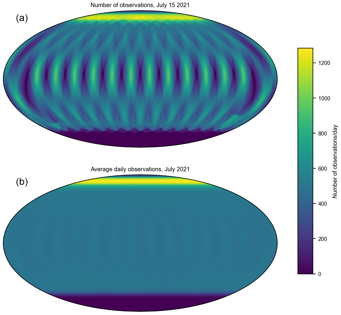
Figure 1 Number of daily observations in each 1^∘ grid box in the MODIS COSP data product, which aggregates only daytime observations, on a single day (a) and averaged over the course of a month (b). Sampling density is illustrated with the number of observations used in determining the cloud mask fraction during July 2021.

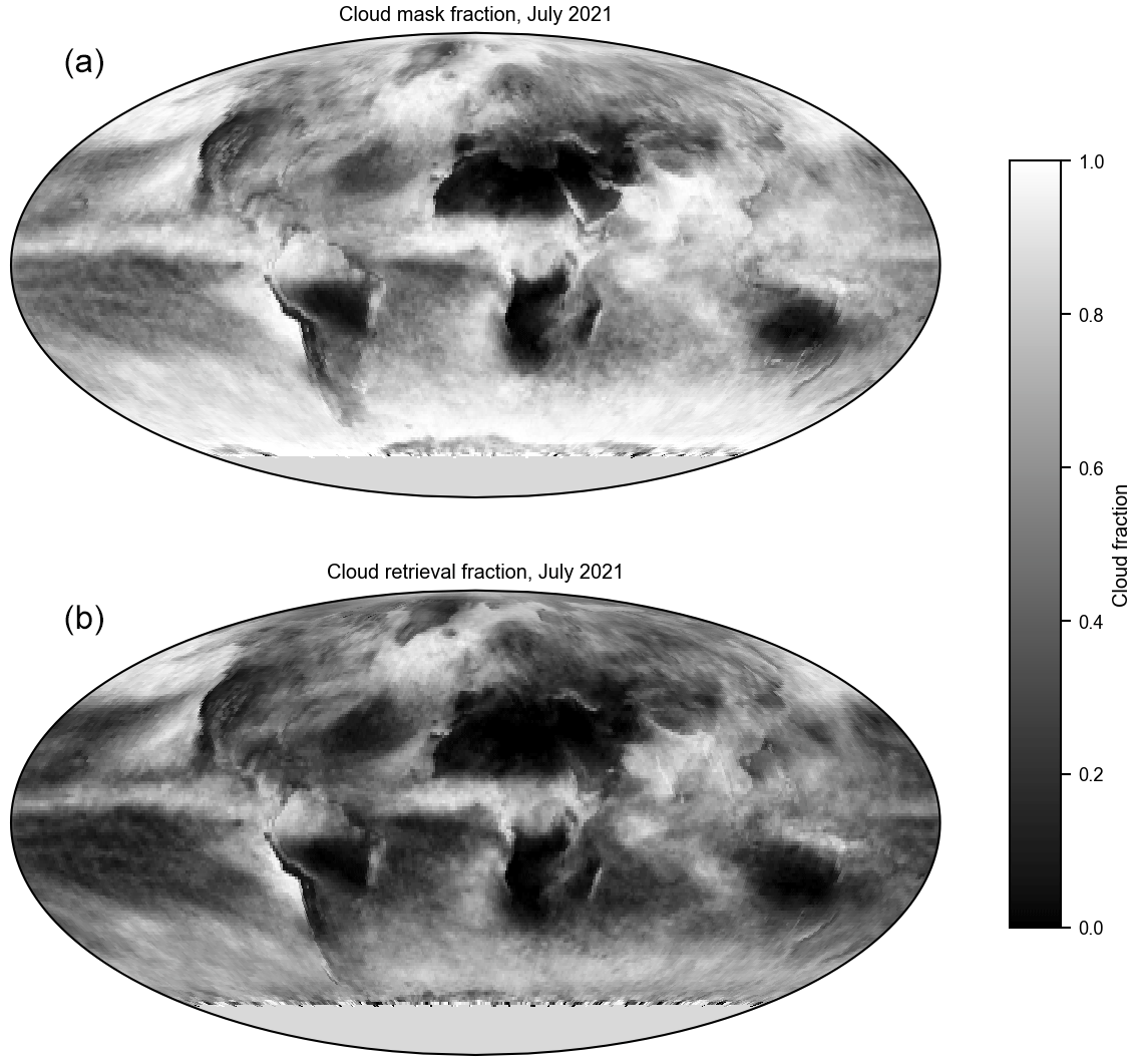
Figure 2 Cloud fraction as determined by the cloud mask (a) and the total determined from the retrievals (b) in July 2021. The cloud mask fraction is the ratio of those pixels for which clouds are probably or confidently detected to the number of pixels for which the cloud mask could be determined. The total cloud retrieval fraction excludes pixels identified as sunglint, heavy aerosol, or partly cloudy. As a result, cloud mask fraction is larger than cloud retrieval fraction almost everywhere, with exceptions only in areas near the wintertime, high-latitude terminator. Each distinct physical quantity in this paper is plotted with a unique color scale.

Starting with Collection 6, standard MODIS Level-3 products (King et al., 2013) use a somewhat involved decision tree aimed at minimizing gaps, overlap, and the aggregation of data from two orbits almost 24 h apart in a single file when deciding which pixels to include in each day's aggregation. Experience with the standard product, however, showed that this decision introduced other artifacts in some fields (especially the cloud fraction from the cloud mask). In the interests of simplicity, the MODIS COSP product reverts to the practice in place before Collection 6; thus, pixels are assigned to days according to the UTC time at the start of the granule's acquisition.

Consistent with standard MODIS datasets, two sets of cloud fraction estimates are produced, with one based on results from cloud detection/masking and a second based on the phase and cloud optical properties determination. Total cloud fraction from the cloud mask is computed by averaging the cloud fraction computed at 5 km scale; as noted in the last section, the 5 km cloud fraction is the ratio of the number of 1 km pixels flagged as probably or confidently cloudy to the number of pixels for which the cloud mask was determined, so that undetermined pixels are not included. Cloud fractions are also computed for high (p_c<440 hPa), middle, and low (p_c≥680 hPa) clouds, based on the determination of cloud-top pressure p_c. The total fraction from the optical property retrieval step is the ratio of the number of pixels for which retrievals were successfully performed to the number of pixels for which the cloud mask was determined (including those pixels for which retrievals could not be performed). Estimates of the fraction of clouds identified as liquid and ice are also provided. The total retrieval cloud fraction includes pixels for which the thermodynamic phase could not be determined and may be larger than the sum of the liquid cloud and ice cloud fractions.

Scalar measures of cloud optical properties for fully cloudy pixels are aggregated in time and space. These properties include cloud optical thickness τ_c and its base 10 logarithm, particle size r_e, and the condensed water path estimated from the product of optical thickness and particle size. The logarithmic mean provides a useful estimate of area mean reflectivity and time mean reflectivity (Pincus et al., 2012). With the exception of the logarithmic mean, scalar measures are also reported separately for partly cloudy pixels. Statistics represent the underlying population so that days with more observations, either because the sampling is denser (Fig. 1) or because clouds are more widespread, contribute more to the time mean than days with fewer observations. This approach differs from the standard MODIS Level-3 product in which monthly means of cloud fraction and cloud-top pressure are the linear average of daily means, tacitly assuming that each day is equally well sampled.

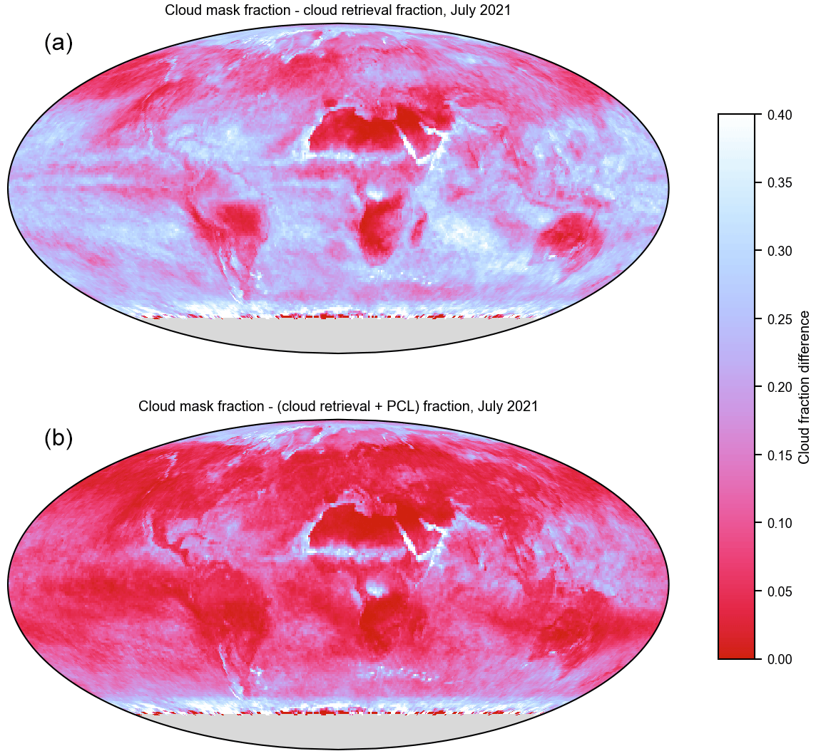
Figure 3 Difference between the cloud fraction determined from the cloud mask and the cloud property retrievals neglecting (a) and including (b) pixels flagged as partly cloudy (PCL) by the clear-sky restoral filtering step in July 2021. The fraction of partly cloudy pixels is computed by summing over the associated joint histogram of cloud optical thickness and cloud-top pressure (Table 2).

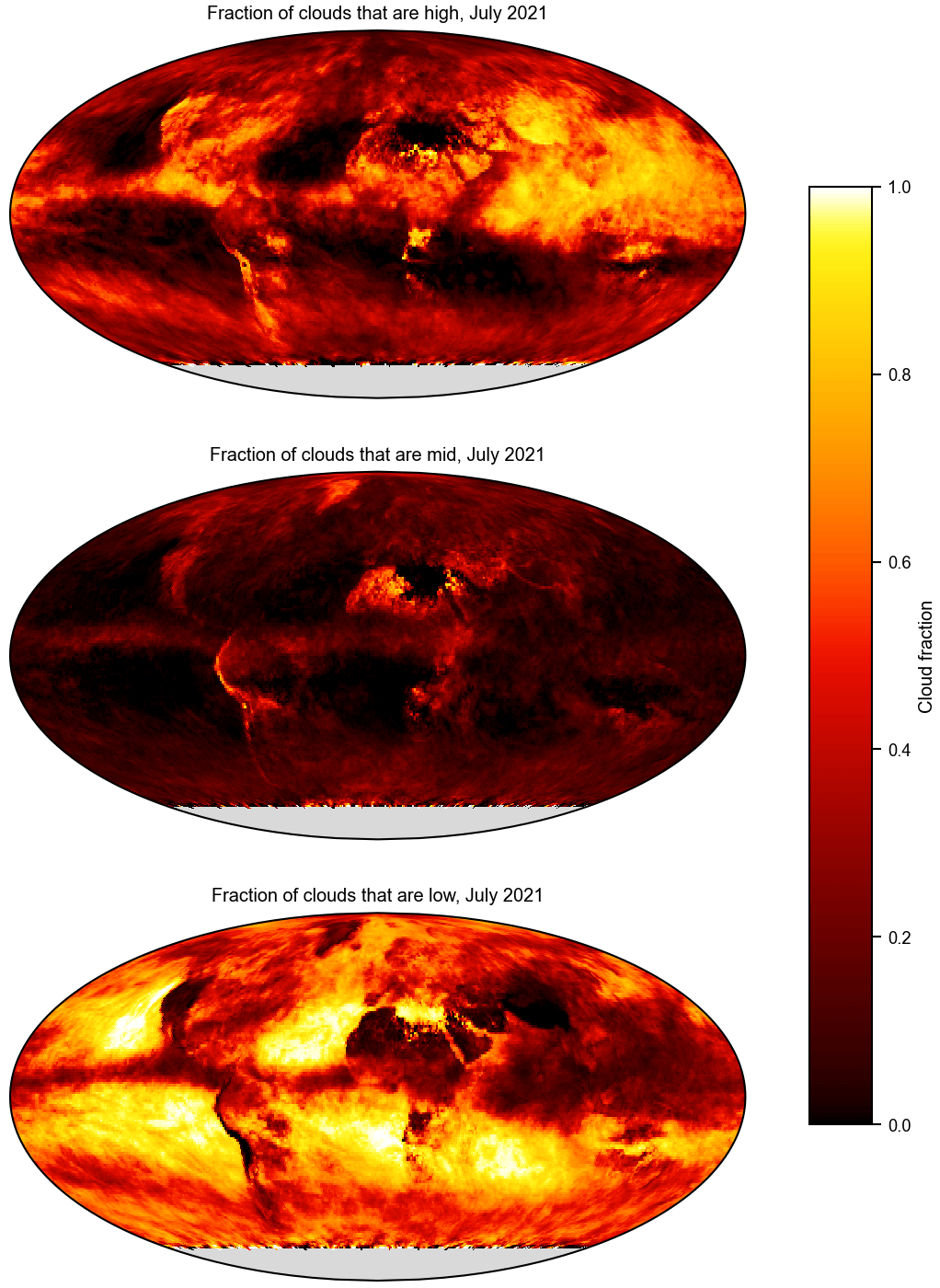
Figure 4 Proportion of clouds determined to be high (cloud-top pressure p_c<440 hPa), mid-level clouds ($\mathrm{680}>p_{\mathrm{c}}\ge \mathrm{440}$ hPa), and low clouds(p_c≥680 hPa) for the month of July 2021.

The dataset also provides joint histograms summarizing the co-variability in cloud optical thickness with cloud particle size (computed separately for liquid and ice clouds) and with cloud-top pressure (separated by phase; for all clouds). Summing the latter over all optical thickness bins and reducing the resolution in cloud-top pressure allows users to compute high, middle, and low cloud fractions consistent with cloud optical properties (as opposed to the cloud mask). Both sets of joint histograms are accumulated for both fully and partly cloudy pixels.

Anticipating increasing interest in the evaluation of aerosol–cloud interactions, the MODIS-COSP dataset also provides joint histograms of the cloud water path and cloud particle size. Such histograms are not yet available from the MODIS simulator within COSP, though we anticipate adding such a diagnostic in the coming months. As with the cloud optical thickness joint histograms, the results are reported separately for fully and partly cloud pixels.

2.2.1 Technical implementation

Although the MODIS COSP dataset MCD06COSP is produced by the MODIS Atmosphere Science Team, it is implemented in a separate data stream from the operational products. Level-2 data are staged to the Atmosphere Science Investigator-led Processing System (SIPS) run by the University of Wisconsin–Madison that supports continuity of data available between MODIS and follow-on sensors, including the Suomi National Polar-orbiting Partnership (NPP). Pixel-scale data are aggregated to Level-3 daily files, and daily files to monthly files, using custom software called Yori, after a character in the 1982 film Tron. Yori accumulates statistics in time and space. Filtering and other transformations are accomplished by adding relevant fields to the Level-2 data. To compute cloud fractions, for example, a field with binary values – 1 where the pixel is considered cloudy by the relevant definition and 0 where the pixel is not – is added to the Level-2 files; in the aggregated Level-3 file, the mean of this field represents the cloud fraction. Cloud fractions resolved by height or phase require fields in which pixels are assigned 1 only when they are cloudy and satisfy the ancillary condition.

Yori computes the mean and standard deviations for each variable. To enable aggregation over time that represents the underlying distributions, Yori also records the sum, sum of squares, and observation numbers for each variable. Yori is also able to compute the joint histogram of two variables. Joint histograms are accumulated as counts (pixels) in each bin and must be normalized before use for most applications.

2.3 Data contents, formatting, and tools for reformatting

Data fields available in the MODIS COSP data are numerated in Tables 1 and 2. Data are produced on a rectangular latitude–longitude grid with 1^∘ spatial resolution. One file combining measurements from both platforms is produced for each day; daily files are accumulated into monthly files, as described above. File names are constructed from a fixed prefix (MCD06COSP), a temporal resolution identifier (D3 or M3, denoting daily or monthly files, respectively), the instrument name, the letter A and the acquisition date as a four-digit year and a three-digit day of year, the collection number, the production date and time, and a file format suffix. As an example, a daily file containing gridded observations from Collection 6.1 from a single day in July 2021 might be MCD06COSP_D3_MODIS.A2021196.062.2022124015916.nc. (Though the observations are drawn from MODIS Collection 6.1, the file name contains “62” due to unfortunate limitations of the file naming at the data distribution facility).

Table 1 Scalar variables available in MODIS COSP files. For each variable, the mean, standard deviation, sum, sum of squares, and number of observations (pixel counts) is reported in each 1^∘ latitude–longitude bin; the latter variables are primarily useful in aggregating over time (e.g., producing monthly files from daily files). Joint histograms are reported as integers and may be normalized by the corresponding number of observations to determine the fractional cloudiness. High clouds are those with cloud-top pressure p_c<440 hPa, mid-level clouds those with $\mathrm{680}>p_{\mathrm{c}}\ge \mathrm{440}$ hPa, and low clouds have p_c≥680 hPa. Total cloud fraction from the cloud mask is 1 minus the sum of probably and confidently clear divided by the total of determined pixels. Total cloud fraction and cloud optical thickness from the cloud retrievals include the clouds in an unknown phase and are determined by assuming a liquid phase. With the exception of the geometric mean optical thickness, all scalar measures of the cloud properties include separate summaries for partly cloudy pixels (i.e., Cloud_Retrieval_Fraction_Total and Cloud_Retrieval_Fraction_PCL_Total), so the total number of data groups is 10 more than the 22 listed below. Corresponding output fields from COSP are prefixed with “modis_” and have closely related names e.g., modis_Cloud_Fraction_Water_Mean and modis_Optical_Thickness_Total_LogMean.

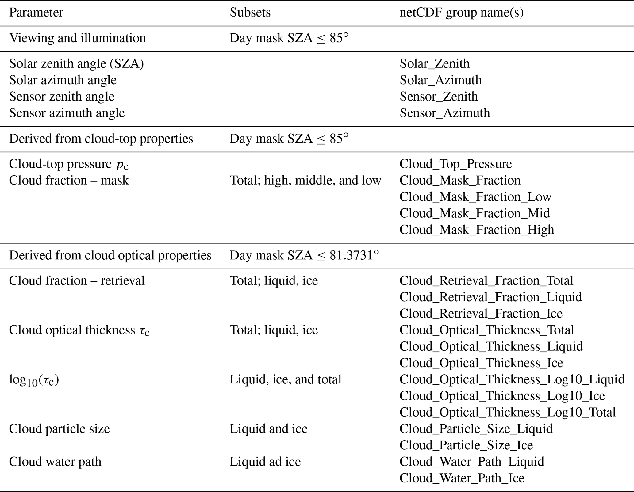
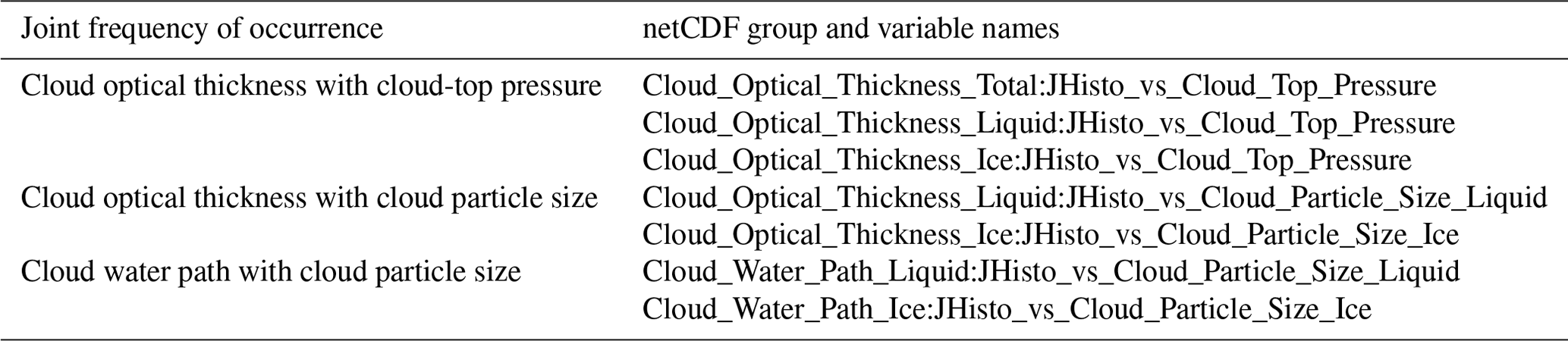
Table 2 Joint histograms available in MODIS COSP files. Joint histograms with particle size are provided for liquid and ice clouds separately; joint histograms with cloud-top pressure are also available for all clouds. Joint histograms of partly cloudy pixels are accumulated separately (e.g., Cloud_Optical_Thickness_Total:JHisto_vs_Cloud_Top_Pressure and Cloud_Optical_Thickness_PCL_Total:JHisto_vs_Cloud_Top_Pressure) so that 14 joint histograms are available in total (see Figs. 7 and 8). Corresponding output fields from COSP are, for example, modis_Optical_Thickness_vs_ReffICE.

The files use netCDF4's ability to organize data into groups. Each netCDF name listed in Table 1 corresponds to one such group, each of which contains variables of Mean, Sum, Sum_Squares, Standard_Deviation, and Pixel_Counts (see Sect. 2.2.1). Six groups also contain joint histograms, i.e., the group Cloud_Optical_Thickness_Liquid contains the variable JHisto_vs_Cloud_Particle_Size_Liquid. Optical thickness and cloud-top pressure are discretized in seven bins in these joint histograms, while particle size is discretized in six bins; the values defining histogram bins are recorded in attributes of the JHisto variable. All variables are functions of latitude and longitude.

NASA distributes the data produced by Yori via the NASA Level-1 and Atmosphere Archive & Distribution System (LAADS) Distributed Active Archive Center (DAAC) in Greenbelt, Maryland, USA. This distribution system imposes some constraints, such as the cryptic file identifier described above. Production with Yori, which was designed for more general purposes, also means that the files may contain more information than needed by most users (e.g., the sum of squares). Finally, satellite data are typically processed month by month, where many applications to climate models will be better served by time series of individual variables. To facilitate comparisons, especially with the MODIS simulator, we have provided Python code that transforms a user-provided set of monthly files containing all variables to datasets with a time series of each variable, which may be written as netCDF files and/or Zarr stores. We have further provided scripts to determine the data available from LAADS and to download it to local storage.

3 What to expect from the data

3.1 Caveats and known issues

An unidentified bug in the cloud mask at Level 2 means a small number of pixels with valid data being ignored. This means the number of valid pixels is sometimes underreported and can occasionally (less than 1 % of the time) even be smaller than the counts for retrievals.

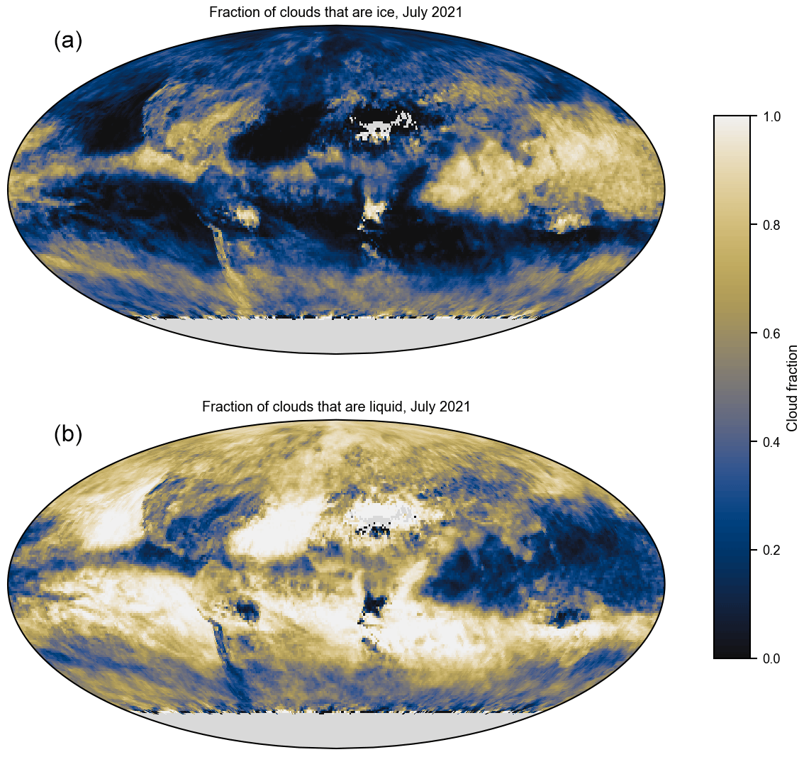
Figure 5 Proportion of clouds for which the thermodynamic phase is determined to be liquid (a) and ice (b) in July 2021. MODIS determines the phase (and uses the relevant cloud microphysical model) for most clouds, where 94 % of the 1^∘ grid cells have less than 5 % of clouds with an undetermined phase during this illustrative month.

As described above, joint histograms (Table 2) of optical thickness and the cloud water path with particle size and of optical thickness with cloud-top pressure are reported as the number of pixels falling in each of the following intervals: (τ;r_e), (CWP;r_e), or (τ;p_c). These may be converted to measures of the cloud fraction in each bin by dividing the number of pixels by the number of observations that might have contributed, i.e., by the Pixel_Counts variable associated with the Cloud_Retrieval_Fraction_Total group.

Because the data derived from the cloud mask use a different threshold for the solar zenith angle (SZA) than fields derived from cloud retrievals, cloud fractions may differ markedly near the terminator (i.e., at the most polar latitudes for which data are available near the equinoxes) for a small proportion (<0.5 %) of the grid cells.

3.2 Measures of cloudiness

3.2.1 Mask and retrieval cloud fractions

As explained in Sect. 2.2, the MODIS COSP Level-3 dataset includes two estimates of cloudiness (cloud fraction), with one computed from the cloud mask and one summarizing the frequency with which cloud properties have been estimated. The two steps have somewhat different aims; the cloud mask seeks to identify pixels unlikely to be clear sky (i.e., filtered for clear-sky retrievals), while the retrieval step seeks to provide accurate estimates of cloud properties and so filters out pixels thought to provide unreliable estimates via clear-sky restoral. The difference between the two estimates for an example month, July 2021, is shown in Fig. 2). The removal of partly cloudy pixels is responsible for much of the roughly 22 % difference. The top panel of Fig. 3 shows the difference between the cloud fraction estimates provided by the mask and the retrievals (i.e., the top and bottom panels of Fig. 2), respectively. The bottom panel shows that the difference is greatly reduced by accounting for the fraction of partly cloud pixels. (Each distinct physical quantity in this paper is plotted with a unique color scale.)

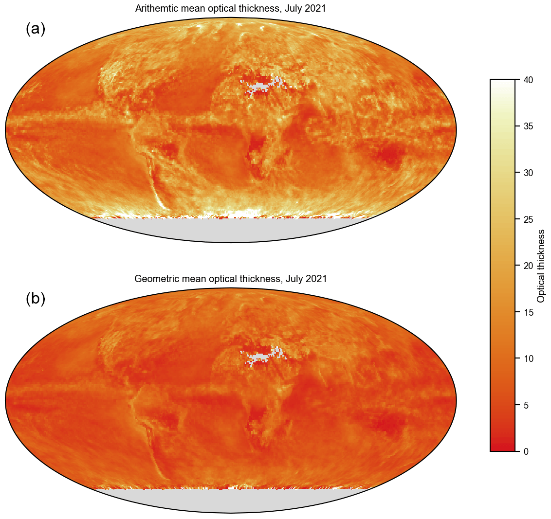
Figure 6 Arithmetic (a) and geometric (b) mean cloud optical thickness for all clouds in July 2021. Geometric mean optical thickness is a better predictor of time-averaged albedo and shows substantially less spatial variation.

3.2.2 Vertical distribution of cloud (mask) fraction

The vertical distribution of total cloudiness, expressed as the proportion of high, middle, and low-topped clouds, is shown for July 2021 in Fig. 4. Cloud-top pressure is at 5 km resolution, where the 1 km cloud mask fraction exceeds 16 % (see Sect. 2.1), so the sum of the three height-resolved clouds fractions is, in some cases, slightly (less than 1 %) smaller than the cloud fraction derived from the cloud mask.

3.2.3 (Retrieval) cloud fraction by phase

As described in Sect. 2.1, the determination of the cloud thermodynamic phase is the first step in the retrieval of cloud optical properties and sets the microphysical model used in reporting these retrievals. Liquid clouds are substantially more common than ice clouds, especially outside the deep tropics (see Fig. 5). Cloud phase is determined for more than 99 % of all fully cloudy pixels, i.e., the total retrieval cloud fraction, which includes pixels for which the thermodynamic phase could not be determined, and is larger than the sum of the liquid and ice cloud fractions by 0.9 % in the global mean. Note that the retrieved phase is weighted toward upper cloud layers when multilayer and multiphase clouds are present (an observational artifact treated by the simulator); i.e., ice cloud layers with significant optical depth overlying lower-level liquid clouds are retrieved as ice.

3.3 Time-averaging: optical thickness and albedo

Though optical thickness is the fundamentally retrieved quantity, its linear average is of limited utility since both albedo (relevant for calculations of shortwave reflectivity) and emissivity (relevant for longwave calculations) depend nonlinearly on optical thickness. The albedo of a distribution of optical thickness is well approximated by the albedo of the geometric mean optical thickness (${\mathrm{10}}^{\stackrel{\mathrm{‾}}{{\log }_{\mathrm{10}}{\mathit{\tau }}_{\mathrm{c}}}}$; Pincus et al., 2012). Figure 6 compares the arithmetic and geometric mean optical thickness for all clouds during July 2021; spatial variations in the latter are substantially smaller.

3.4 Joint distributions

Both the MODIS and ISCCP simulators produce joint histograms of cloud optical thickness τ_c and cloud-top pressure p_c, though the difference between the simulators is not as marked as the difference between the observations (Pincus et al., 2012), where the CO₂ slicing used by MODIS assigns more clouds to lower pressures than the temperature-based characterization from ISCCP does. The MODIS-COSP dataset further resolves the histograms by thermodynamic phase and for fully and partly cloudy pixels (Table 2). Global mean (area-weighted) histograms are shown in Fig. 7. The vast majority of partly cloudy pixels turn out to be liquid, very low (p_c>800 hPa), and optically thin (τ_c≤3.6), suggesting that the algorithms used to identify these pixels are performing as designed.

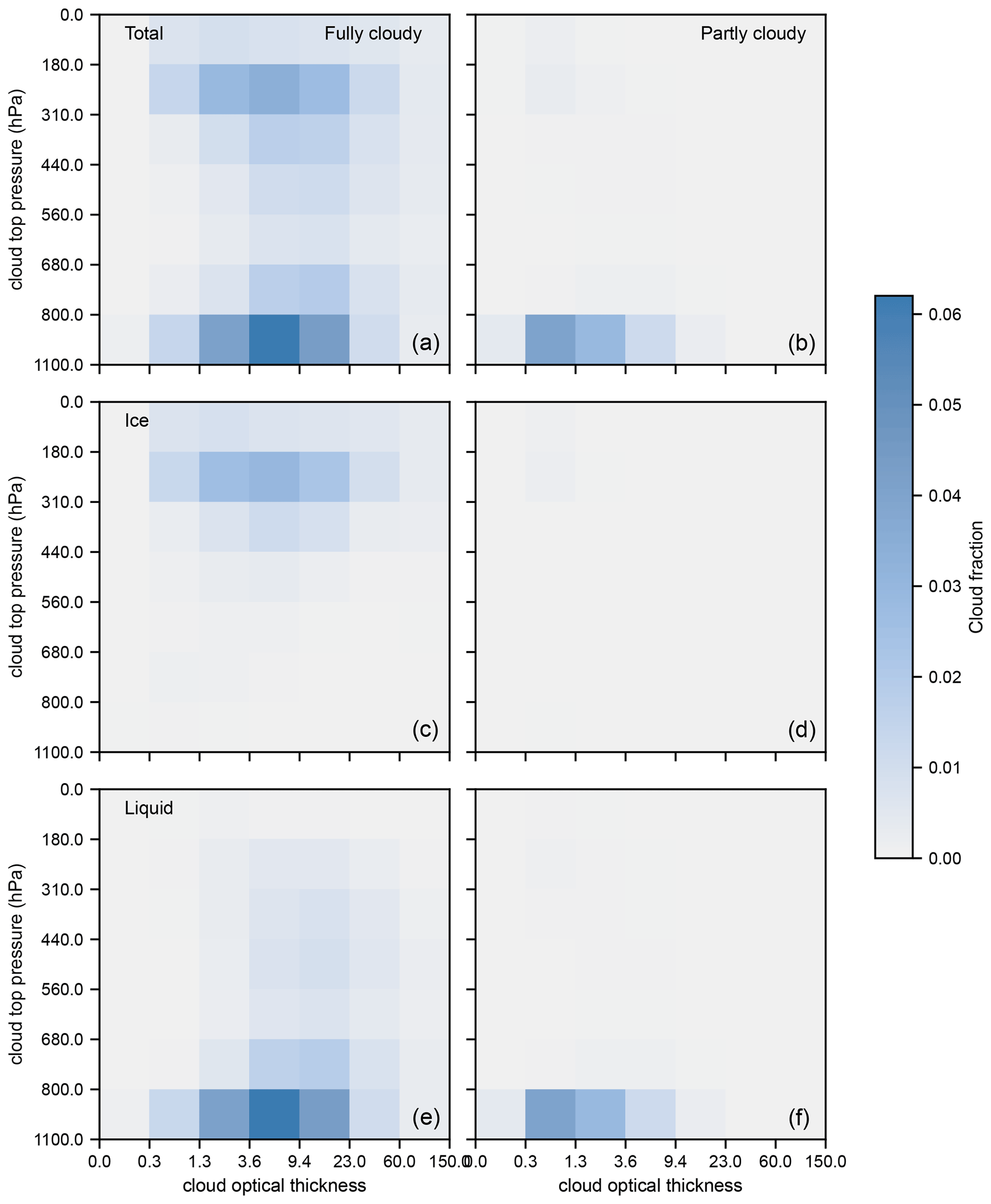
Figure 7 Joint frequency of cloud optical thickness (τ_c; x axis) and cloud-top pressure p_c (y axis), shown as global (area-weighted) means for July 2021. Panels (a) and (b) are for total cloudiness, panels (c) and (d) show ice clouds, and panels (e) and (f) show liquid clouds, respectively. Panels (a), (c), and (e) show the results for fully cloudy pixels, while panels (b), (d), and (f) show partly cloudy pixels.

Global mean joint histograms of τ_c with particle size r_e are shown in Fig. 8. Optical thickness is accumulated in the same bins as the τ_c–p_c histograms, which themselves follow ISCCP conventions; particle size bins are spaced unevenly to resolve spatial and temporal variations. The observations span the entire range of possible particle size values for both liquid and ice clouds in both the fully and partly cloudy populations of pixels.

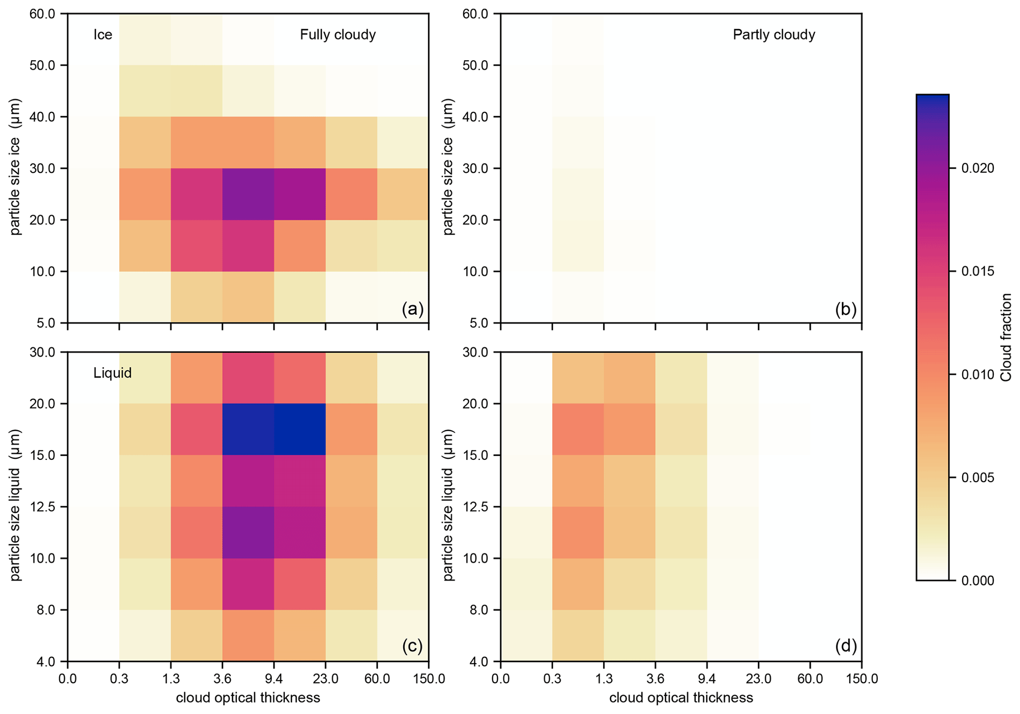
Figure 8 Joint frequency of cloud optical thickness (τ_c; x axis) and effective particle size r_e (y axis), shown as global (area-weighted) means for July 2021. Ice clouds are in panels (a) and (b) and liquid clouds in panels (c) and (d). Fully cloudy pixels are in panels (a) and (c) and the much smaller number of partly cloudy pixels are in panels (b) and (d). Bins of optical thickness (x axis) are spaced quasi-logarithmically; the particle size bins are non-uniform in an attempt to resolve the variations. Partly cloudy pixels tend to be optically thin, especially for ice (see also Fig. 7), with particle sizes spanning the same range as the fully cloudy pixels.

MODIS retrievals are formulated in terms of optical thickness and particle size (see Sect. 2.1), but the appropriately scaled product of these quantities is used to estimate the cloud (liquid or ice) water path for each pixel (Platnick et al., 2017). The MODIS-COSP datasets provide joint histograms of these values with particle size to support studies of aerosol–cloud interactions, where the ability to disentangle aerosol impacts on the particle size from the impacts on the cloudiness and water path may be valuable. Figure 9 shows an example of these histograms averaged over the globe for a single month. These histograms are not yet available from the MODIS simulator, but we expect to add the capability to produce them in the coming months.

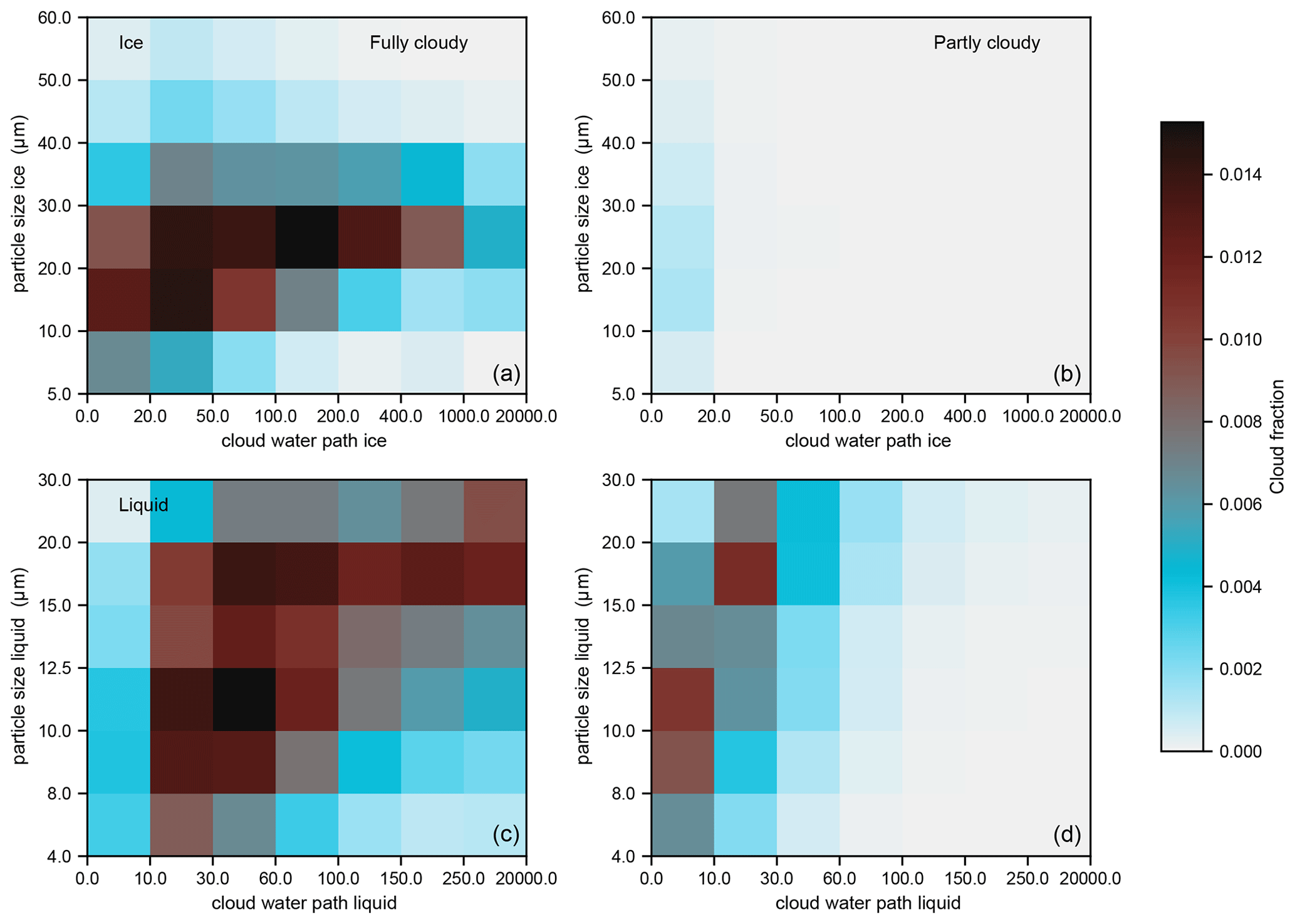
Figure 9 Joint frequency of cloud water path and cloud particle size, shown as global (area-weighted) means for July 2021, with thermodynamic phase in rows and fully/partly cloudy pixels separated by column.

4 Code and data availability

The data described in this paper are available for download from the NASA Level-1 and Atmosphere Archive & Distribution System (LAADS) Distributed Active Archive Center (DAAC) in Greenbelt, Maryland, USA. The daily data may be cited as https://doi.org/10.5067/MODIS/MCD06COSP_D3_MODIS.062 (NASA, 2022b). The citation for the monthly data is https://doi.org/10.5067/MODIS/MCD06COSP_M3_MODIS.062 (NASA, 2022a).

The code used to create the figures in this paper, including code for downloading and post-processing the data and making the figures themselves, is available at https://doi.org/10.5281/zenodo.7883987 (Pincus, 2023).

5 Comparing the data with the MODIS simulator and other MODIS datasets

5.1 Differences with respect to standard Level 3

The MODIS COSP Level-3 dataset MCD06COSP is provided as a technical convenience to users of COSP and the MODIS simulator. Differences relative to the standard MODIS Level-3 products, described throughout this paper, may be summarized as follows:

1. The dataset contains observations from both the Terra and Aqua platforms.

2. Height-resolved cloud fractions from the cloud mask are reported.

3. Cloud fractions for liquid and ice clouds, as determined by the cloud optical properties processing, are reported.

4. Joint histograms of cloud optical thickness with effective radius are reported more compactly.

5. Data are restricted to daytime observations.

6. All scalars represent the underlying population of pixels, while the temporal averages of the cloud mask and cloud-top pressure datasets in the standard Level-3 products weight each day equally.

7. Data are provided in netCDF4 files.

5.2 Comparisons to the MODIS simulator

The MODIS simulator does not attempt to emulate the separate cloud identification and cloud retrieval steps described in Sect. 2.1 but instead identifies cloudy pseudo-pixels based on a threshold for (true) visible wavelength optical depth (Pincus et al., 2012). In particular, there is no equivalent in the proxy to the quite different cloud mask and cloud retrieval fractions produced by MODIS. The majority of this difference is caused by partly cloudy pixels (see Fig. 3), for which there is no analogy in COSP. The data described here lower the technical barriers to comparisons between simulator and observations, but the conceptual issues, described in Pincus et al. (2012), remain.

The MODIS simulator, like COSP as a whole, operates on single atmospheric states. Aggregation over time, in addition to any attempt to account for orbital sampling, is the responsibility of the host model and is typically performed as the simulation advances. We stress that the MODIS-COSP data are designed to represent the underlying population of cloudy pixels observed in each region over the course of a day or month, so that mean values represent the in-cloud mean and not the domain mean. This implies that the implementation of the MODIS simulator in host models must be the mean values weighted by the relevant instantaneous simulator-produced cloud fraction within the climate model to be directly comparable to the monthly dataset reported here. Users might alternatively choose to compute their own monthly mean observations, weighting each day equally, from the daily data.