The enhanced future Flows and Groundwater dataset: development and evaluation of nationally consistent hydrological projections based on UKCP18

This paper details the development and evaluation of the enhanced future FLows and Groundwater (eFLaG) dataset of nationally consistent hydrological projections for the UK, based on the latest UK Climate Projections (UKCP18). The projections are derived from a range of hydrological models. For river flows, multiple models (Grid-to-Grid, PDM (Probability Distributed Model) and GR (Génie Rural; both four- and six-parameter versions, GR4J and GR6J)) are used to provide an indication of hydrological model uncertainty. For groundwater, two models are used, a groundwater level model (AquiMod) and a groundwater recharge model (ZOODRM: zooming object-oriented distributed-recharge model). A 12-member ensemble of transient projections of present and future (up to 2080) daily river flows, groundwater levels and groundwater recharge was produced using bias-corrected data from the UKCP18 regional (12 km) climate ensemble. Projections are provided for 200 river catchments, 54 groundwater level boreholes and 558 groundwater bodies, all sampling across the diverse hydrological and geological conditions of the UK. An evaluation was carried out to appraise the quality of hydrological model simulations against observations and also to appraise the reliability of hydrological models driven by the regional climate model (RCM) ensemble in terms of their capacity to reproduce hydrological regimes in the current period. The dataset was originally conceived as a prototype climate service for drought planning for the UK water sector and so has been developed with drought, low river flow and low groundwater level applications as the primary objectives. The evaluation metrics show that river flows and groundwater levels are, for the majority of catchments and boreholes, well simulated across the flow and level regime, meaning that the eFLaG dataset could be applied to a wider range of water resources research and management contexts, pending a full evaluation for the designated purpose. Only a single climate model and one emissions scenario are used, so any applications should ideally contextualise the outcomes with other climate model–scenario combinations. The dataset can be accessed in Hannaford et al. (2022): https://doi.org/10.5285/1bb90673-ad37-4679-90b9-0126109639a9.

1 Introduction

This paper details the development and evaluation of the enhanced future FLows and Groundwater (hereafter referred to as “eFLaG”) dataset of nationally consistent and spatially coherent hydrological (river flow and groundwater) projections for the UK, based on UKCP18 – the latest climate projections for the UK from the UK Climate Projections programme (Murphy et al., 2018). eFLaG provides a successor to the Future Flows and Groundwater Levels (FFGWL) dataset (Prudhomme et al., 2013), which was based on the UKCP09 projections (Murphy et al., 2009).

The eFLaG dataset was developed specifically as a demonstration climate service for use by the water industry for water resources and drought planning and hence by design is focused on future projections of drought, low river flows and low groundwater levels. By providing a consistent dataset of future projections of these variables, eFLaG can potentially support a wide range of applications across other sectors. The predecessor, FFGWL, has been widely used within the water industry but has also found very wide application for diverse research purposes (see Sect. 9).

As in FFGWL, in eFLaG the climate projections are used as input to a range of hydrological models to provide nationally consistent, spatially coherent projections of river flow and groundwater levels for the 21st century. The use of an ensemble of river flow models also provides information on hydrological model uncertainty. As well as using an updated set of climate projections, eFLaG capitalises on advances in national-scale river flow and groundwater modelling since FFGWL and detailed evaluation of the applicability of models for drought simulation, notably research under the NERC Drought and Water Scarcity (DWS) programme (e.g. Rudd et al., 2017; Smith et al., 2019).

Previous research on hydrological projections

There is a long history of climate change impact assessment within the UK water industry and academia, which we do not review in detail here. Watts et al. (2015) provide an overview of past research (up to around 2013) on climate projections relevant for the water sector, including for future water resources and drought. More recently, Chan et al. (2022) provided an in-depth review of the evolution of the use of climate change projections for hydrological applications. Here, we briefly address some pertinent developments in river flow projections since FFGWL.

The original FFGWL did not present an assessment of future drought risk, other than seasonal river flows (Prudhomme et al., 2012) and groundwater levels (Jackson et al., 2015), which suggested pronounced decreases in future summer flows, reductions in annual-average groundwater levels, and increases (decreases) in winter (summer) groundwater levels. Since then, the original FFGWL projections have been used in a number of hydrological impact studies. Collet et al. (2018) presented a probabilistic appraisal of future river flow drought (and flood) hazard in the UK showing hydro-hazard “hotspots” in western Britain and north-eastern Scotland, especially during the autumn. Hughes et al. (2021) used the zooming object-oriented distributed recharge model (ZOODRM) distributed groundwater recharge model to assess changes in 21st century seasonal recharge across river basin districts and groundwater bodies in the UK based on the FFGWL climate change projections. The results showed a consistent trend of more recharge being concentrated over fewer months, with increased recharge in winter and decreased recharge in summer.

In addition to UKCP09 and FFGWL, other datasets have been developed using different global climate model (GCM)–regional climate model (RCM)–hydrological model chains. One major development has been the use of large ensemble projections of future climate variables from the Weather@Home RCM (specifically HadRM3P) as part of the MaRIUS (Managing the risks, impacts and uncertainties of drought and water scarcity) project within the DWS programme (Guillod et al., 2018). The MaRIUS projections provide large ensembles (100+) of past, present (1900–2006) and future (2020–2049 and 2070–2099) climate outputs. These were used as inputs to the national-scale Grid-to-Grid (G2G) hydrological model to provide a similarly large gridded (1 km²) dataset of river flow and soil moisture (Bell et al., 2018). Analysis of these datasets has been conducted for drought (Rudd et al., 2019) and low flows (Kay et al., 2018), indicating future increases in hydrological drought severity and spatial extent and decreases in absolute low flows.

A further source of hydro-meteorological projections now available is that from the EDgE (End-to-end Demonstrator for improved decision-making for the water sector in Europe) project; see Samaniego et al. (2019). EDgE delivered an ensemble comprising two GCMs and four “impact” models (gridded land surface and hydrological models at a 5 × 5 km scale) for the whole of Europe. Visser-Quinn et al. (2019) analysed future river flow drought risk in this ensemble using a similar approach to Collet et al. (2018) and found similar results in terms of the spatial distribution and magnitude of future changes in droughts, albeit with some differences arising from the use of different scenarios, GCMs and hydrological models.

While such products may be used for climate adaptation research, the most relevant for eFLaG is the release of UKCP18. To date, relatively few studies using UKCP18 have been published. Kay et al. (2020) made a rapid assessment of UKCP18 impacts on hydrology compared to UKCP09. More recently, Kay (2021), Kay et al. (2021a, b, c), Lane and Kay (2021) and Kay (2022) provided future assessments of potential changes in seasonal mean river flows, high flows and low flows using various UKCP18 products with the G2G hydrological model. They found potential increases in winter mean flows and high flows and decreases in summer and low flows, albeit with wide uncertainty ranges. In the literature to date, and to the authors' knowledge, there have been no published assessments of future groundwater levels or groundwater recharge using UKCP18 – although groundwater levels driven by UKCP18 are currently being used in the latest operational water resources management plans (e.g. Thames Water, 2023).

In summary, there have been substantial scientific advances in hydrological projections for the UK since Watts et al. (2015) and FFGWL, including some research on future indicators relevant for water resources availability and drought. However, relatively few datasets have been made available to the community since FFGWL. While MaRIUS and EDgE provide complementary hydrological datasets, there remains a need for an accessible dataset based on UKCP18. Existing UKCP18 studies have been focused on time-slice projections and/or have used a single hydrological model (e.g. Kay et al., 2021a, b, c), so there will be significant benefit arising from the eFLaG dataset of transient projections from a range of hydrological models covering river flows, groundwater levels and groundwater recharge.

2 Outline of the dataset and overview of the modelling chain

In the following sections we set out the methodology behind the eFLaG dataset. This section firstly provides a brief overview of the various stages of the methodology and how our method samples the “cascade of uncertainty” (Smith et al., 2019) emerging from the multiplicity of projections and other modelling choices. While the original FFGWL methodology provided an initial foundation for eFLaG, much has changed in the decade since that study was commissioned, and the new UKCP18 projections differ from UKCP09 (e.g. Kay et al., 2020). eFLaG therefore required the development of a new methodology, which is described in detail in the following sections.

The whole project workflow is illustrated in Fig. 1. eFLaG is driven by the UKCP18 dataset, specifically the “Regional” 12 km projections, to which a bias correction is applied. Section 3 describes the processing of the climate projections, including the bias-correction method. The UKCP18 projections are used as input to three river flow models, i.e. GR (Génie Rural), PDM (Probability Distributed Model) and G2G, one groundwater level model (AquiMod) and one groundwater recharge model (ZOODRM), to provide simulations for 200 river catchments, 54 groundwater boreholes and 558 groundwater bodies respectively. Section 4 provides more detail on how these sites were selected. Details of the hydrological models and their calibration are given in Sect. 5. The evaluation of the models is covered in Sects. 6 and 7. Figure 1 also illustrates how all of the eFLaG projections feed into a series of water industry demonstrators, in partnership with UK water providers (specifically, Dwr Cymru/Welsh Water and Thames Water). These are not discussed in detail in this paper, but they were relevant for the site selection and as such are mentioned briefly below.

Figure 1 Project workflow illustrating the stages of analysis described in this paper.

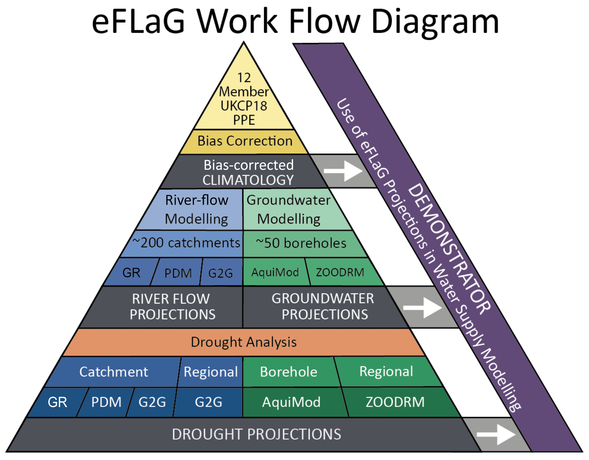
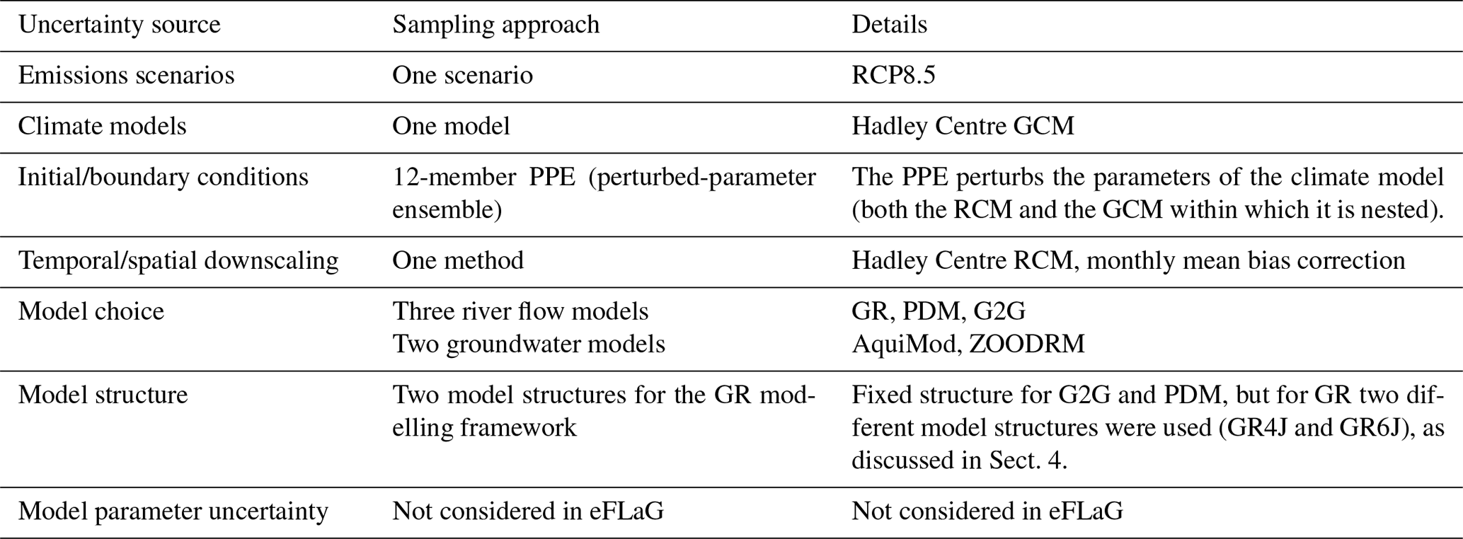
The question of uncertainty in climate impact modelling is a challenging one that has been explored in a whole range of studies extending back to the 1980s, when climate projections began to be routinely produced. There are inherent uncertainties at every step of the process, including climate emissions scenarios, climate modelling, environmental modelling (in our case hydrological modelling, which itself has a vast literature when it comes to uncertainty estimation) and wider impact modelling (e.g. in water supply systems). Recently, Smith et al. (2018) presented this issue as a “cascade of uncertainty” (using widely adopted terminology, e.g. Wilby and Dessai, 2010). Within eFLaG, as with the majority of climate impact applications, it is not possible to sample across all sources of uncertainty. We adopted a pragmatic approach to sampling key sources of uncertainty within the available time and resources constraints. In Table 1, we consider the sources of uncertainty and our approach to sampling from them. The focus in eFLaG is on uncertainty arising from initial/boundary conditions. Additionally, for the river flow simulations, the uncertainty arising from model choice is also accounted for, embracing models of different types (lumped and distributed) and structures. The effect of different structures of the same model is also included through the use of two versions of one of the models (namely the GR suite).

Table 1 Sources of uncertainty explored in eFLaG (building on the framework of Smith et al., 2018).

3 UKCP data processing

The UKCP18 regional climate projections were created using perturbed-parameter runs of the Hadley Centre global climate model (GCM, HadGEM3-GC3.05) and regional climate model (RCM, HadREM3-GA705) (Murphy et al., 2018). These provide a set of 12 high-resolution (12 km) spatially consistent climate projections over the UK, covering the period December 1980–November 2080. The 12-member RCM perturbed-parameter ensemble (PPE) is valuable for representing climate model parameter uncertainty; ensemble members are numbered 01–15, excluding 02, 03 and 14 (as there are no RCM equivalents for these GCM PPE members: Murphy et al., 2018, Sect. 4.3), and 01 is the standard parameterisation. However, it is important to note that, as all ensemble members are based on the same high-emissions scenario (RCP8.5) and the underlying climate model structure, they do not represent the full climate uncertainty. The UKCP18 RCM output was processed to provide the variables needed for hydrological modelling, namely 1 km gridded and catchment-average time series of available precipitation (i.e. after the application of a snow module; see below) and potential evapotranspiration (PET), not itself a UKCP18 output but estimated using available UKCP18 variables as described below.

The Hadley Centre climate model uses a simplified 360 d year consisting of 12 30 d months. The RCM precipitation and temperature time series are given for this 360 d calendar and are therefore not consistent with the $\mathrm{365}/\mathrm{6}$ d observed time series. Previously, the FFGWL Climate project inserted 5 (or 6 in a leap year) days of zero rainfall into the RCM time series, so that the observed and RCM data were using comparable calendars (Prudhomme et al., 2012). However, here the data were kept in the 360 d format to avoid modifying the time series with artificial data.

3.1 Precipitation

Daily precipitation time series were available for each of the UKCP18 RCM–PPE members. However, the RCM data showed biases compared to observed precipitation, as is common for climate data (Murphy et al., 2018; Teutschbein and Seibert, 2012). The RCM data substantially overestimate precipitation for most months (typically by around 1 mm d⁻¹ for the UK mean, Murphy et al., 2018, Fig. 4.4), the exception being August–October. A simple monthly-mean bias-correction methodology was therefore applied through the following steps.

1. The 1 km HadUK-Grid observed rainfall product was averaged to 12 km for consistency with the RCM data (Hollis et al., 2019).

2. For each month and grid cell, change factors were calculated between the RCM-simulated precipitation and observation-based HadUK-Grid time-slice mean of monthly total rainfall over the period 1981–2010. This resulted in bias-correction factor grids being made for each month and each RCM ensemble member, as shown in Fig. 2.

3. The change-factor grids were then smoothed to reduce spatial discontinuities by updating each grid cell using a weighted combination of the original grid-cell value and neighbouring values, as in Guillod et al. (2018).

4. To produce bias-corrected precipitation estimates, the RCM-simulated precipitation time series were multiplied by the bias-correction factor grid for each month (i.e. all January precipitation was multiplied by the January bias-correction grids, February precipitation by the February correction grid, etc.).

The bias-corrected precipitation products were then downscaled from 12 to 1 km based on the distribution of the standard average annual rainfall (SAAR) for the period 1961–1990, as in previous studies (Bell et al., 2007; Kay and Crooks, 2014). This involved calculating the ratio of the observed SAAR at 1 km to the observed SAAR averaged up to the 12 km RCM grid and then multiplying RCM precipitation values by this ratio. This introduces further spatial variability related to typical rainfall patterns, but the total rainfall across the original 12 km RCM grid cell remains unchanged.

3.2 Accounting for snowmelt processes

A simple snow module was applied to account for snowmelt processes (Bell et al., 2016). The snow module converted the 1 km bias-corrected precipitation into rainfall plus snowmelt (i.e. available precipitation) based on temperature. This used the minimum and maximum daily temperatures provided by each RCM ensemble member, which were first scaled from a 12 km resolution to 1 km using a lapse rate based on elevation data. The parameters used in the snow module are given in the Supplement (Table S1).

3.3 Potential evapotranspiration

PET was not directly available as an RCM output and was therefore generated using a range of variables from the RCM–PPE climate time series (Table S2). The PET was calculated using the same methodology as the Hydro-PE dataset (Robinson et al., 2021, 2022), except for the use of eFLaG bias-corrected precipitation data within the interception correction component. This produces Penman–Monteith PET parameterised for short grass. The equation also included monthly stomatal resistance values, which were adjusted for the future period to account for the impact of increased carbon dioxide concentrations on stomata (as in Rudd and Kay, 2016, based on Kruijt et al., 2008). The PET data were then copied down from a 12 to 1 km resolution by simply setting all 1 km grid cells to the value of the containing 12 km grid cell.

3.4 Outputs

The 1 km gridded time series of “available precipitation” and PET were then used to produce the time series of catchment averages required for each of the eFLaG river catchments and groundwater boreholes. For the river catchments, the catchment-average values were derived using the standard UK National River Flow Archive (NRFA) approach for catchment-average rainfalls, as described in the NRFA (2021). For the boreholes, following Mackay et al. (2014a), averages were taken over the representative aquifer length, which was determined as the groundwater flow path between the borehole and a single discharge point on a river based on the catchment geometry and hydrogeology. For the grid-based models, ZOODRM and G2G, the gridded data were used directly.

The bias-corrected climate outputs are part of the eFLaG dataset described further in Sect. 8. For each river catchment and groundwater borehole, bias-corrected data are available for the observational period, for the purposes of evaluation of the hydrological model outputs and for the future. In addition, the gridded bias-corrected climatology is made available as a separate dataset (Lane and Kay, 2022; see also the Data availability section).

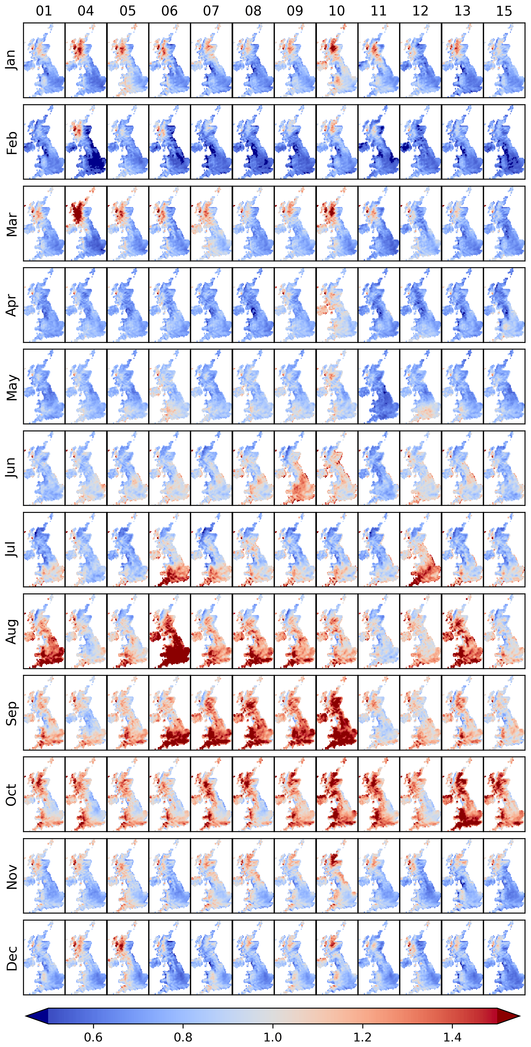
Figure 2 Bias-correction grids applied to correct monthly precipitation. Values are correction factors used to modify precipitation, with a value of 0.5 halving precipitation, 1 meaning no change to precipitation, 2 doubling precipitation, etc. The columns show the results from each RCM–PPE member, and the rows show the results for each month. Note that the column numbers reflect the RCM–PPE number (see Sect. 3).

4 Catchment selection

The UK is fortunate to have one of the densest hydrometric networks in the world, with a legacy of strong commitment to data quality and completeness. There are more than 1500 river flow gauging stations with flow records in the NRFA (Dixon et al., 2013, and https://nrfa.ceh.ac.uk/, last access: 29 March 2023) and more than 180 observation boreholes with groundwater level records in the BGS National Groundwater Level Archive (NGLA). These archives are the principal sources of validated river flow and groundwater level data at the UK scale. A remit of the NRFA and NGLA is to archive data that are useful for a wide variety of applications, primarily focusing on the most strategically important records. However, such catchments are not always the most relevant for the water industry, and water companies often have their own sites on which they undertake analysis. Since the eFLaG project aims to maximise utility for a range of users, the catchment selection strategy considered both research and industry needs.

Detailed site lists and metadata for river flow, groundwater level and groundwater recharge are catalogued on the dataset held at the Environmental Informatics Data Centre (EIDC) (Hannaford et al., 2022).

4.1 River flows

To support selection, a meta-database was assembled for all NRFA gauging stations in the UK, primarily using the NRFA's metadata holdings published on the NRFA website and in the UK Hydrometric Register (Marsh and Hannaford, 2008). Metadata compiled included membership of key national strategic networks (e.g. the near-natural Benchmark Network (UKBN2; Harrigan et al., 2018a) and operational monitoring networks), capitalising on efforts of other projects in quality-controlling data and ensuring catchments are fit for purpose. Selection also considered whether catchments were used in previous relevant projects that have simulated river flows for drought analysis. The selection ensured a strong representation of the original FFGWL catchments (with 117 catchments featuring in both) and also overlap with recent modelling endeavours through the DWS programme (AboutDrought, 2021) projects Historic Droughts, IMPETUS (Improving predictions of drought to inform user decisions) and MaRIUS, which used several of the models used by eFLaG (specifically G2G and GR4J – Génie Rural à 4 paramètres Journalier). In this regard we ensured that 165 eFLaG catchments overlapped with at least one DWS project.

Selection also focused on data quality. Longer record lengths were prioritised and hydrometric quality was evaluated where possible. Given the extent of hydrometric issues (at low flows especially), it is not possible for all sites to have the highest-quality data, but where decisions were made on similar sites, quality was considered a tiebreaker. The selection included 80 Benchmark catchments but did not seek to focus entirely on natural catchments given the limited range of variability they capture (being mostly small and clustered in headwaters) and also included large and disturbed sites known to be important for water industry purposes. Artificial influences are prevalent across the UK and have been shown to prominently affect flow regimes (e.g. Rameshwaran et al., 2022) and drought characteristics (Tijdeman et al., 2018) in many catchments. Hence, the incorporation of a range of Benchmark near-natural catchments and artificially influenced sites is important for ensuring representativeness and demonstrating the utility of the different models used, which treat artificial influences differently (Sect. 5). Membership of the Benchmark catchments is highlighted in the dataset description, and information on artificial influences can be accessed for all sites on the NRFA website (in station descriptions and “Factors Affecting Runoff” codes).

Catchment representativeness was also considered, enabling the eFLaG dataset to sample the hydrological variability of the UK. Representativeness was considered by comparing the distribution of eFLaG potential selections relative to various catchment descriptors from the NRFA Hydrometric Register (altitude, area, annual rainfall, baseflow index, land cover, etc.).

Finally, this activity focused on ensuring water industry relevance. At the national scale, this was achieved by asking stakeholders at an eFLaG workshop for views on additional catchments (Durant and Counsell, 2021). In this way, 12 catchments were added. Similarly, for the regional demonstrators (Dwr Cymru/Welsh Water and Thames Water), water company teams were consulted to gain a better understanding of strategically important flow records for water companies in the case study regions, leading to an additional five catchments.

The final eFLaG dataset consists of 200 catchments (Fig. 3a) giving good geographical coverage and representativeness of the UK.

4.2 Groundwater levels

Boreholes were selected to ensure a number of essential criteria were met. Firstly, only those boreholes with the highest-quality records of groundwater level were considered. This required regular (at least monthly) and continuous (at least 10 years in length) records of data from boreholes that are in zones which are not significantly affected by groundwater abstraction.

Secondly, sites were chosen to ensure coverage of the UK's principal aquifers where possible, enabling the eFLaG dataset to sample the hydrogeological variability of the UK. This broadly aligns with the requirements of other national-scale assessments of groundwater resources undertaken as part of the original FFGWL project and the Historic Droughts and IMPETUS projects. Accordingly, the selection aimed to ensure good coherence with these studies too.

Thirdly, as with river flow catchment selection, an additional activity focused on ensuring water industry relevance, at the national scale, through both consultation with stakeholders at the eFLaG workshop and through consultation with key demonstrator partners (Dwr Cymru/Welsh Water and Thames Water), who identified strategically important boreholes that would strengthen the outputs for long-term drought-risk assessment to support the water resources planning case study. Through this activity, several additional boreholes were identified.

These selection criteria identified over 70 “candidate” boreholes for the eFLaG project. A final quality-assurance procedure was then undertaken, whereby a preliminary analysis of AquiMod's ability to capture low groundwater levels was undertaken at each borehole via visual inspection of the simulated hydrographs. A final set of 54 boreholes was selected (Fig. 3b). They represent a significant advance in aquifer coverage compared to the 24 NGLA boreholes used in FFGWL, 15 of which are used in both.

4.3 Groundwater recharge

The gridded groundwater recharge simulations have been aggregated over 558 “groundwater bodies” covering England (Environment Agency, 2021a), Wales (Natural Resources Wales, 2023) and Scotland (Ó Dochartaigh et al., 2015) (Fig. 3c). These units were used for two principal reasons. Firstly, they are physically justifiable as they reflect known hydrogeological characteristics, including groundwater recharge and groundwater flow regimes, so that each catchment represents a distinct body of groundwater that can reasonably be considered in isolation. Secondly, they are coherent with the licensing areas defined as part of Catchment Abstraction Management Strategy (Environment Agency, 2021b) and management areas for the implementation of the Water Framework Directive. They are, therefore, directly relevant to water regulation and the wider water industry.

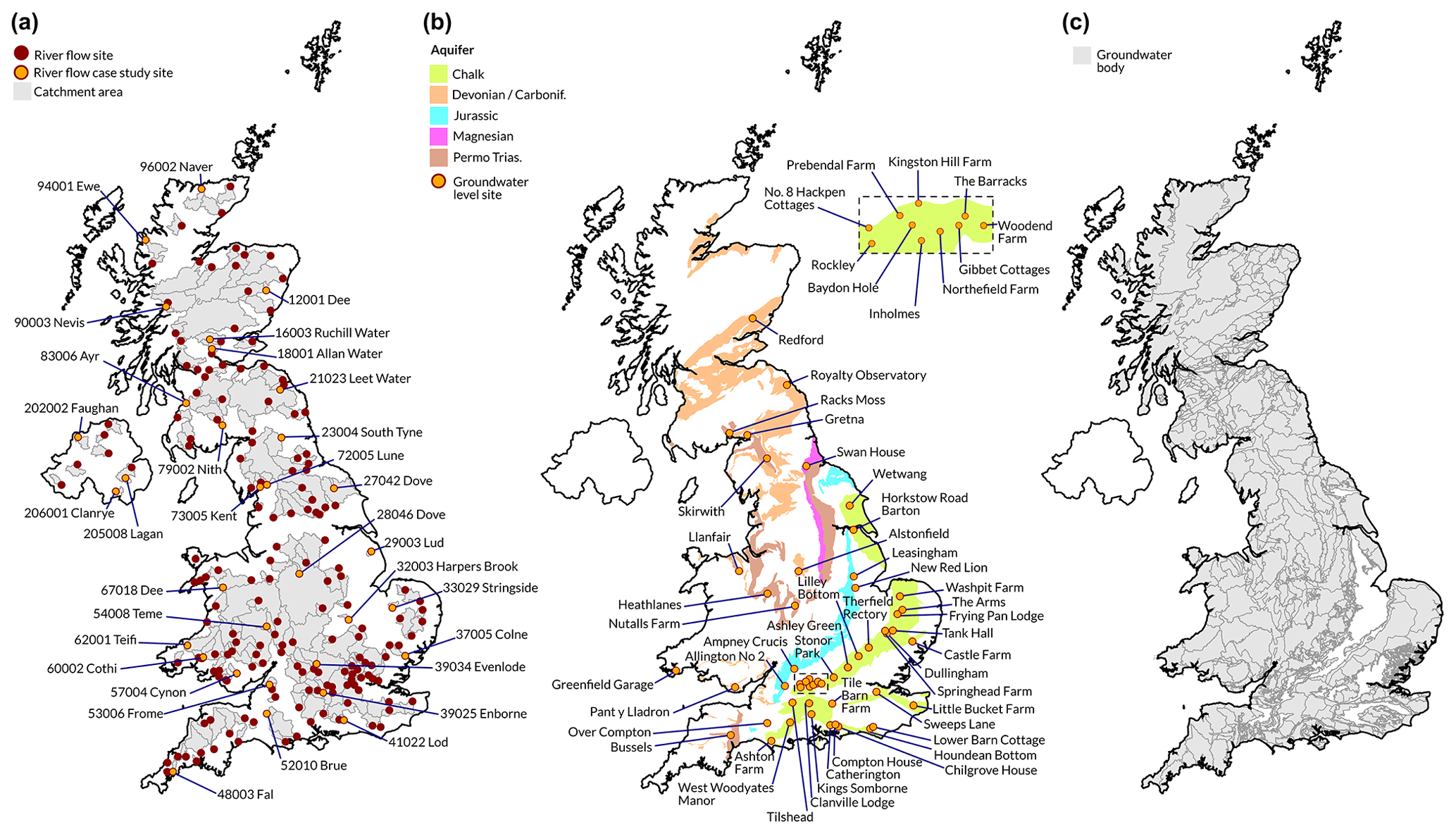
Figure 3 (a) Map of the 200 eFLaG catchments highlighting those used as case study sites in Sect. 7. (b) Map of 54 eFLaG boreholes and principal UK aquifers, including the Chalk, Devonian and Carboniferous aquifers (Devonian/Carbonif.), Jurassic limestones (Jurassic), Magnesian limestones (Magnesian) and Permo-Triassic sandstones (Permo Trias.). (c) Map of 558 groundwater bodies. The inset of Fig. 3b shows the Berkshire downs, where there are a high number of boreholes.

5 Hydrological and groundwater model ensemble set-up

Creation of an eFLaG dataset is underpinned by hydrological and groundwater models used to transform rainfall and PET to river flow, soil moisture, groundwater levels and recharge. The approach builds on that employed under FFGWL (Prudhomme et al., 2013) whilst exploiting developments in hydrological modelling for droughts since that time.

For modelling of river flows, eFLaG used two lumped catchment models, PDM (Moore, 2007) and the GR suite (Perrin et al., 2003), and one distributed grid-based hydrological model, G2G (Bell et al., 2009). PDM was used in FFWGL and therefore provides some comparability with that project. Embracing a range of different model structures and spatial representations can provide insights into how assessments of future river flows (and hence drought or low-flow risk under climate change) are sensitive to hydrological model choice. It should be noted that an important difference between the river flow models is in the treatment of artificial influences (abstractions and discharges). G2G is not calibrated and simulates natural river flows only (i.e. it does not include artificial influences). The GR suite and PDM do not explicitly include artificial influences either, but as calibrated models they will implicitly include the net effect of artificial influences in the simulations. We return to this important distinction in the results and discussion.

For groundwater, eFLaG adopted the lumped, conceptual, AquiMod groundwater model (Mackay et al., 2014a) to simulate groundwater level time series on a daily time step at the boreholes identified in Sect. 4. AquiMod was the groundwater level model used in FFGWL providing direct comparison. In addition to groundwater levels, ZOODRM (Mansour and Hughes, 2004) was used to study changes in future groundwater recharge.

In the following sub-sections, we describe each of these models in turn, providing information on the model set-up, calibration and past approaches to evaluation. A consistent approach was applied to the model application and evaluation across all these models where possible. However, it is important to emphasise that, while some aspects were common, insofar as possible (e.g. model-driving data), it was necessary to apply different approaches to suit the model in question. Calibration was done according to past applications and best practice. Hence, the calibration approach described below is similar for the GR suite and PDM but different for AquiMod, and by its nature, G2G requires no specific calibration here. Where calibration was carried out for the conceptual models, it was undertaken for the full period of record of available data.

Identical approaches to evaluation were adopted across all river flow models, but minor differences applied to groundwater, as described below.

There are two sets of model output in eFLaG described below – this terminology is adopted throughout.

• simobs. observation-driven simulation (i.e. simulations for the observed period, driven by observational climate datasets, described below). The simobs period varies between models but covers at least the January 1961–December 2018 period.

• simrcm. UKCP18 RCM-driven simulation (12 ensemble members) (i.e. simulations driven by the UKCP18 RCM bias-corrected dataset as described in Sect. 3). These are available for 1980 to 2080. The simrcm runs from the observed period could then be evaluated against the simobs data.

Common driving data were applied across all the models for the simobs runs. Accepted national-standard observational climate products were used, including the following.

• Precipitation and temperature: the HadUK-Grid 1 km × 1 km dataset (Hollis et al., 2019), the national-standard gridded meteorological dataset and observational product associated with UKCP18

• PET: MORECS (Meteorological Office Rainfall and Evaporation Calculation System) (Hough and Jones, 1997) is an established, national gridded PET product. Other PET datasets such as CHESS (Robinson et al., 2016) and more recently the Environment Agency's PET product (Environment Agency, 2021c) have been available, but the decision to use MORECS was based on the availability of data for the whole of the UK.

For all the models, evaluation was undertaken in two stages, which is typical practice for appraising a model for simulation of climate-change impacts.

1. Evaluation when driven with baseline-observed climate data

2. Evaluation when driven with baseline climate model data

Stage 1 involves the use of evaluation statistics to assess the performance of model simulations driven by observed climate data (the simobs runs) against observations of river flow and groundwater. For Stage 1, a range of metrics is available and widely used to assess how well rainfall–runoff or groundwater models perform against observations. Within eFLaG, these metrics were used to assess performance (Table 2). For river flows, these metrics have a focus on low-flow metrics (e.g. Nash–Sutcliffe efficiency, NSE, on log-transformed flows), but some do evaluate performance across the flow regime. For groundwater levels, a generalised NSE score was used which provides an overall assessment of process realism and fit to groundwater level data. The simulated and observed Standardized Groundwater level Index (SGI) was also compared using the NSE (NSE_SGI), which focuses on groundwater extremes, including droughts.

It is not possible to do a thorough evaluation of the recharge simulations from ZOODRM, given the difficulty in measuring recharge, particularly at a scale that is commensurable with a national model. However, past applications of ZOODRM (e.g. Mansour et al., 2018) have successfully used monthly river flow data as a means of evaluating ZOODRM's ability to capture catchment water balances and infer the accuracy of seasonal recharge simulations (further details are provided in the model description). Accordingly, a sub-set of the river flow metrics relevant to monthly river flows has been used to evaluate ZOODRM for Stage 1.

Table 2 Model calibration and evaluation metrics used in eFLaG.

^* One-hundredth of the mean observed flow was added to both modelled and observed flow values during evaluation in order to avoid errors and biases due to very small and zero flows.

Sources of quality-controlled, long-term observational data for model calibration and evaluation were the national-standard repositories for hydrological data.

• River flows: UK National River Flow Archive: https://nrfa.ceh.ac.uk/ (last access: 29 March 2023)

• Groundwater levels: UK National Groundwater Level Archive: https://www2.bgs.ac.uk/groundwater/datainfo/levels/ngla.html (last access: 29 March 2023)

Stage 2 appraises the performance of the models when driven by the climate model outputs. That is, it compares the simobs and simrcm runs over the common baseline period. This assessment cannot use performance metrics based on time series, as climate models are not expected to reproduce the sequencing of events seen over the historical period (Kay et al., 2015). Instead, the comparison has been done in terms of river flow and groundwater level duration curves, low-flow/low-level metrics and seasonal recharge values, thus comparing the statistical characteristics of river flows, groundwater levels and groundwater recharge rather than their day-to-day equivalence (Kay et al., 2015, 2018). When looking at the performance of an ensemble of climate model runs, the model simulation driven by observed data would ideally sit within the range covered by the ensemble (assuming an ensemble of sufficient size). However, it would not necessarily be expected to sit in the middle of the ensemble range, because the set of weather events that actually occurred within the historical observed baseline period is just one realisation of what could have occurred within the range of natural variability (Kay et al., 2018).

5.1 Description of the models and the specific set-up

5.1.1 GR4J/GR6J

The GR4J (Génie Rural à 4 paramètres Journalier) and GR6J (Génie Rural à 6 paramètres Journalier) models come from a suite of hydrological models provided in the airGR modelling suite (Coron et al., 2021) for the R software program. Both models are well suited to application across many catchments using the inbuilt automatic parameter optimisation function. The simple, efficient forms of airGR models also make them suitable for uncertainty and ensemble analyses.

GR4J is a simple daily lumped conceptual model with only four free parameters. GR4J has been used for hydroclimate change research across the globe and has demonstrated good performance in a diverse set of catchments in the UK. The model has been applied in the UK for operational seasonal forecasting and for long-term drought reconstructions nationwide (Harrigan et al., 2018b; Smith et al., 2019).

GR6J (Pushpalatha et al., 2011) is a six-parameter variant of the GR modelling suite that was developed to improve low-flow simulation and groundwater exchange. Recently, GR6J has increasingly been applied in UK water resources applications (e.g. Anglian Water, 2021).

For eFLaG, it was decided, therefore, that using both GR4J and GR6J would be beneficial. Both GR4J and GR6J were calibrated using the inbuilt automatic calibration function, with the modified Kling–Gupta efficiency (KGE, Gupta et al., 2009; Kling et al., 2012) as the error criterion (“ErrorCritKGE2”). KGE offers a thorough error criterion as it calculates the correlation coefficient, the bias and the variability between simulated and observed flows. KGE values range from −Inf to 1, with 1 being a perfect fit. The calibration algorithm was applied to square-root-transformed flows in order to place weight evenly across the flow regime. The airGR snowmelt module CemaNeige was not applied, as a simple snow module was applied to the climate data to pre-process the precipitation data into rainfall and snowmelt based upon temperature (See Sect. 3).

5.1.2 Grid-to-Grid

The G2G hydrological model is an established model distributed area-wide that has been used to investigate the spatial coherence and variability of floods and droughts at catchment, regional and national scales. Model output typically consists of natural river flows at both gauged and ungauged locations and can be provided as time series for specific locations as well as 1 km × 1 km grids. G2G has been used for climate impact modelling of floods (Bell et al., 2009, 2012), low flows (Kay et al., 2018) and droughts (Rudd et al., 2019) and is also used operationally for flood forecasting (Cole and Moore, 2009; Moore et al., 2006).

G2G is typically configured on a 1 km × 1 km grid across Great Britain using spatial datasets of landscape properties such as soil type and drainage network, together with a few nationally applied model parameters. The model is thus parameterised using national-scale spatial datasets (e.g. soil grids) rather than via individual catchment calibration. The spatial datasets and parameters used here are the same as those used in previous studies (Rudd et al., 2019; Bell et al., 2009, 2012; Kay et al., 2018). Note that model output for G2G is for 186 of the 200 eFLaG catchments. Of the 14 catchments excluded, 9 are in Northern Ireland and so are not covered by the version of G2G applied here. For the other five catchments there were difficulties in identifying appropriate outlet locations on the 1 km network of flow directions used by G2G.

G2G can either be initialised with model water stores set to default or zero values or from a states file appropriate to the run start date. In eFLaG the G2G was run for 2 years with observed rainfall and PET to provide a 1 January 1963 states file to initialise the observation-driven G2G model run. The RCM-driven G2G runs were all initialised with a generic December states file provided by an obs-driven run (for 1 December 1980), and then the first 2 years of each RCM-driven run were discarded to allow for model spin-up. The eFLaG river flow datasets therefore cover the periods 1 January 1963 to 31 December 2018 (simobs) and 1 December 1982 to 30 November 2080 (simrcm).

5.1.3 PDM

PDM (Moore, 2007; UKCEH, 2022) is a simple, very widely used lumped rainfall–runoff model that can be configured to a variety of catchment flow regimes. Within the model, a soil water store with a distribution of water absorption capacities controls runoff production through a saturation excess process; stored water is also lost to evaporation. In one configuration, all runoff enters a surface store (the fast pathway), while a groundwater store (the slow pathway) is recharged by soil water drainage. In an alternative configuration, the runoff is split between the two stores according to a fixed fraction. Water in the surface water and groundwater stores is routed using a non-linear storage equation (powers of 1, 2 and 3 were trialled under eFLaG) or, for the surface store, a cascade of two linear reservoirs before being combined to produce the modelled flow at the catchment outlet. Water is conserved within the model, whilst a multiplicative factor (equal to 1 if not required) is applied to the input precipitation. Alternatively, a groundwater extension (Moore and Bell, 2002) may be invoked to allow modelling of underflow at the catchment outlet, external springs, pumped abstractions and incorporation of well-level data. Multiple hydrological response zones within a catchment can also be represented (not trialled under eFLaG). PDM may be thought of as a toolkit of model components representing a range of runoff-production and flow-routing behaviours and with a choice of time step.

Under eFLaG, single-zone PDM models were invoked with a daily time step. The model stores were initialised using the mean observed flow over the period of record and the first 2 years of model flow discarded to allow for model spin-up. Nineteen different combinations of the above-mentioned toolkit options were systematically trialled for each catchment. Parameter estimation was performed using an automatic calibration procedure that applied a simplex optimisation scheme (Nelder and Mead, 1965) to increasing numbers of model parameters in turn. The rainfall factor, or, when employed, a spring factor (representing net water exchange for the catchment), were used to achieve zero bias in the modelled flows with respect to observations. The remaining parameters were estimated so as to optimise the modified Kling–Gupta efficiency calculated on either the square-root-transformed flows or, to a limited extent, the log-transformed flows (see “Supplementary information 2” in the Supplement).

5.1.4 AquiMod

AquiMod is a lumped conceptual groundwater model that links simplified equations of soil drainage, unsaturated zone flow, and saturated groundwater flow to simulate daily groundwater level time series at a specified borehole (Mackay et al., 2014b). Each of these three components uses model parameters that describe site-specific hydrological and hydrogeological characteristics of the groundwater catchment surrounding the borehole. The model also has a flexible saturated-zone model structure that can be modified to represent different levels of vertical heterogeneity in hydrogeological properties.

For each borehole, the AquiMod parameters and structure were calibrated to achieve the most efficient simulation of available historical groundwater level data using NSE, which provides a reliable assessment of overall process realism and goodness of fit to groundwater level time series; following the approaches of Mackay et al. (2014a) and Jackson et al. (2016), model parameters that could be related to catchment information (e.g. relating to known land cover and soil type) were fixed. The remaining parameters were then calibrated using six different saturated-zone model structures, including a one-layer model (fixed hydraulic conductivity and specific yield), two- and three-layer models with variable hydraulic conductivity and fixed specific yield, two- and three-layer models with variable hydraulic conductivity and variable specific yield and a “cocktail glass” representation of hydraulic conductivity variation with depth (William et al., 2006). The optimal structure–parameter combination was obtained for each borehole using the shuffled complex evolution global optimisation algorithm.

The calibrated models were then evaluated for their ability to capture groundwater level extremes using the SGI (Bloomfield and Marchant, 2013) as the basis for this evaluation. The SGI is a normalised index, calculated directly from groundwater level time series, which can be used to identify droughts and provide a quantitative status of groundwater resource drought events (e.g. Bloomfield et al., 2019).

5.1.5 ZOODRM

ZOODRM is a distributed recharge calculation model originally developed to estimate recharge values to drive groundwater models (Mansour and Hughes, 2004). It is applied over the British Mainland using a 2 km square grid. The FAO Drainage and Irrigation Paper 56 (FAO, 1998) approach, modified by Griffiths et al. (2006), is used to calculate potential recharge. This method removes actual evaporation and soil moisture deficit from rainfall and calculates potential recharge as a fraction of the excess water using a runoff coefficient value. The model was driven by daily rainfall and potential evaporation data. The model was primarily parameterised using available national-scale data, including data relating to the soil hydrology (Boorman et al., 1995), vegetation (Land Cover Map 2000; NERC, 2000) and surface topography. The latter of these was used to route surface water runoff.

The runoff coefficient, which defines the proportion of excess soil water that drains overland via surface runoff, is an unknown parameter which must be calibrated. This was done in two stages. Firstly, the calibration problem was simplified by defining zones of equal runoff coefficients. In total, 35 zones were used in ZOODRM, which were based on UK hydrogeological and geological maps (DiGMapGB-625, 2008). Then, the runoff coefficient for each zone was manually calibrated by comparing simulated runoff to observed river flows minus baseflow, which was calculated using a well-established baseflow separation method (Gustard et al., 1992). This was done using monthly mean flows given that ZOODRM does not have a sophisticated runoff routing scheme, and it is not expected, therefore, to capture daily variability in runoff. The comparison to monthly flows does, however, provide a useful means of evaluating the seasonal water balance of the model which serves as the best available proxy for the accuracy of the recharge simulations. In total, 41 gauging stations were used to assess the model performance.

The only hydrological process that needs initialisation in the ZOODRM is the soil moisture deficit. As all simulations start in January, which is a wet month with minimal potential evaporation, it is assumed that the initial soil moisture deficit is equal to zero. Even so, a warm-up period of 1 year is used to initialise the model.

6 Hydrological model evaluation (Stage-1 evaluation)

This section provides a brief summary of the outputs of the Stage-1 evaluation. Note that, for river flows, model evaluation was undertaken at the same gauged locations and for the same period of time used for model calibration, except for G2G, which is not specifically calibrated.

6.1 River flows

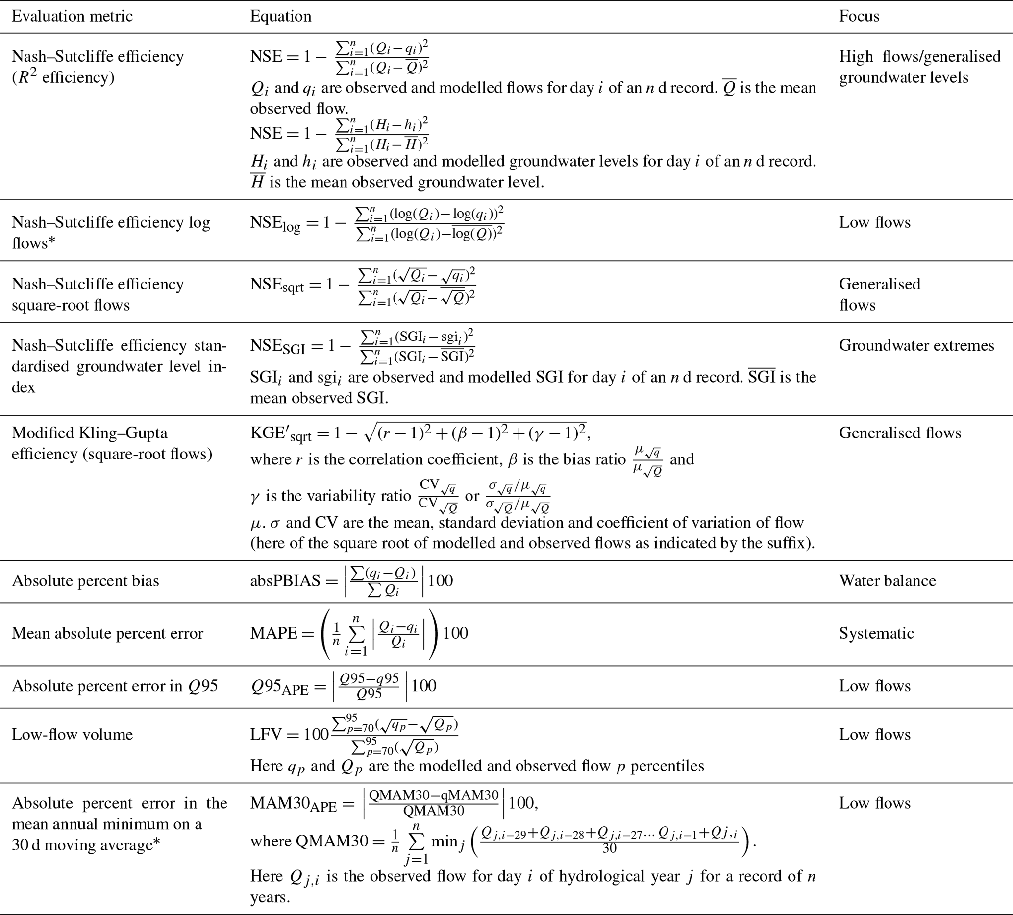
Figure 4 summarises the range of Stage-1 evaluation metrics across all the catchments, while Supplement Figs. S2 to S5 provide maps of the evaluation metrics at each catchment. For GR4J, generally there was good performance across performance metrics in most catchments. Some outliers are present in the drought metrics, particularly in the south-east and London. For GR6J, we observed good performance across all performance and drought metrics. GR6J generally performs slightly better than GR4J, particularly as shown in low-flow catchments in the logNSE metric. For PDM, very good scores are obtained across the 200 sites, especially the low-flow/drought indicators (bottom rows).

For G2G, again, good performance was observed overall (medians for NSE/logNSE/sqrtNSE/KGE2 ≥0.7). However, the performance was generally lower than for GR or PDM because the G2G is not calibrated to individual catchments, and G2G simulates natural flows, whereas the lumped models are calibrated to the observations used for performance assessment. In catchments with a high degree of anthropogenic disturbance, G2G is less able to simulate observed flows, whereas the calibration of the other hydrological models will implicitly account for such artificial impacts, meaning they are inevitably more likely to replicate observed flows even if these processes are not included explicitly.

This distinction highlights an important benefit of eFLaG: PDM and GR4J/GR6J are calibrated to present-day flows, and hence simulated flows are not natural, as they implicitly include artificial impacts. These runs do not, therefore, allow users to separate natural flows and artificial influences in the baseline period or to project how they may change relative to each other in the future. On the other hand, although not used here, G2G has the capability of including artificial influences separately (e.g. Rameshwaran et al., 2022). We return to this issue in Sect. 9.

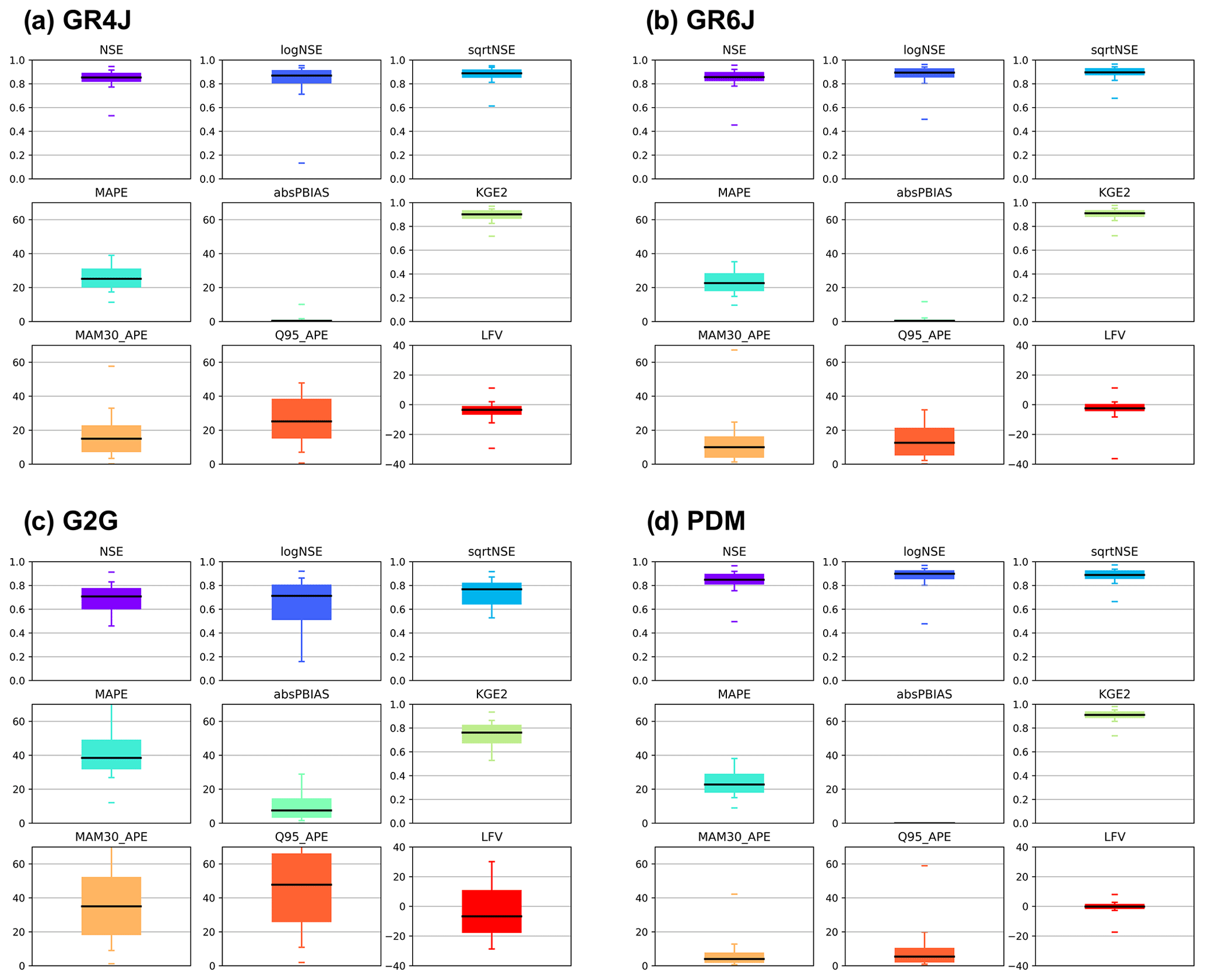
Figure 4 Evaluation of modelled river flow performance. The key evaluation metrics outlined in Table 2 are summarised for all 200 modelled catchments (GR4J, GR6J, PDM) or 186 modelled catchments (G2G).

In general, the eFLaG dataset shows a very good range of performance comparable with previous applications of these models for the UK (e.g. Rudd et al., 2017; Harrigan et al., 2018b; Smith et al., 2019). There are some commonalities with these previous studies in terms of spatial patterns. Rudd et al. (2017) also noted that G2G performance is likely to reflect the fact that simulated flows are natural (hence performance is poorer in the south and east, where artificial influences are typical greater). Issues with poorer performance in groundwater-dominated catchments were highlighted for GR4J by Smith et al. (2019), and the present study shows that eFLaG enables some improvement through GR6J. Smith et al. (2019) also highlighted how a lack of snowmelt constrained performance in some areas (e.g. north-eastern Scotland), while the current results also show improvements in these areas in eFLaG, given the inclusion of snowmelt accounting.

6.2 Groundwater levels

Figure 5 summarises the model evaluation results for the 54 AquiMod models used in eFLaG. The results show that all 54 models demonstrate good overall efficiency in capturing daily groundwater level dynamics, achieving NSE ≥0.77. All but 11 of the models achieve NSE ≥0.85, and 28 of the models achieve NSE ≥0.90. These include all seven models situated in the Permo-Triassic sandstone and four out of five of the models situated in the Devonian and Carboniferous aquifers. Swan House and Lower Barn Cottage, the only models situated in the Magnesian limestones and Lower Greensand respectively, achieved NSE values of 0.82 and 0.86. The Chalk and Jurassic limestone borehole models span the full range of NSE scores.

The results show that all 54 AquiMod models are able to capture the historical SGI time series efficiently, achieving NSE_SGI ≥0.6, which indicates that the models effectively capture groundwater extremes, including periods of drought. The majority of the models show a lower NSE_SGI compared to the NSE, although several models show a negligible difference. On average, the NSE_SGI is 0.15 less than the NSE.

Figure 5 AquiMod evaluation metric results including NSE (a) and NSE_SGI (b).

6.3 Groundwater recharge

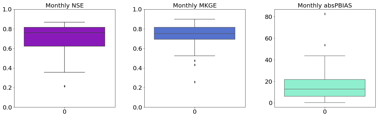
ZOODRM demonstrates an ability to efficiently capture monthly mean river flows as reflected by the medians for NSE and KGE2, which both exceed 0.75, and the median absolute percent bias, which is 12.7 % (Fig. 6). Figure S6 shows the distributed recharge model results at the 41 gauging stations across the country. The model uses a simplistic overland routing approach, which is implemented to check the water balance on a monthly basis, noting that large-scale spatial recharge values are most commonly used to drive groundwater flow models using monthly stress periods.

Figure 6 Distributed recharge model ZOODRM evaluation results.

7 Evaluation of RCM-based runs in the baseline (Stage-2 evaluation)

This section briefly considers the outcomes of the Stage-2 evaluation, focusing firstly on flow/groundwater duration curves for a sub-set of eFLaG sites (see map, Fig 3) and then specifically on the representation of particular low flows (low groundwater level) quantiles.

7.1 Flow-duration curves

Flow-duration curves (FDCs) summarise the entirety of the flow regime from high to low flows by including all river flows and expressing them in terms of the percentage of time a given flow is exceeded. Figures 7 and S7 to S9 provide a perspective on the ability of the RCM-driven river flow simulations (simrcm) to replicate the range and frequency of flows based on the observation of climate-driven river flow simulations (simobs). FDCs are shown for a common baseline period of 1989–2018.

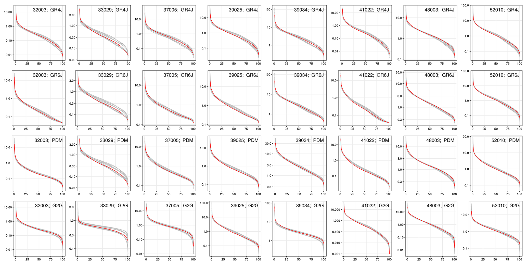
Figure 7 Flow-duration curves (FDCs) comparing the baseline flow regime in the 12 RCM ensemble members (simrcm, grey lines) to simulated observed ones (simobs, red line), 1989–2018. FDCs are featured for four hydrological models (GR4J, GR6J, PDM, G2G; rows) and eight catchments in southern and eastern England (32003 Harpers Brook, 33029 Stringside, 37005 Colne, 39025 Enborne, 39034 Evenlode, 41022 Lod, 48003 Fal, 52010 Brue; columns). The y axis represents river flows (cumecs) on a logarithmic scale.

The close correspondence between FDCs derived from the RCM ensemble members and model observations suggests that the RCM ensemble performs well in replicating flows across the regime. This is consistent across most UK catchments, illustrated by the representative sub-set of 32 catchments featured in Figs. 7 and S7 to S9. The model observations are usually within the range of values from the 12 ensemble members throughout the flow regime. There are some catchments for which the RCM ensemble is more likely to overestimate the lowest half of the flow regime (exceedance probabilities of 50–100), most notably for Stringside (33029; Fig. 7), Dove (28046; Fig. S7), Frome (53006; Fig. S8) and Lud (29003; Fig. S7).

For certain catchments such as Stringside (33029; Fig. 7) and Lud (29003; Fig. S7), although there appears to be greater RCM uncertainty in river flows than for other catchments, the differences tend to be exaggerated in smaller, drier catchments with lower flows across the flow regime. The logarithmic y axis is also a contributing factor to this and also accounts for the seemingly larger RCM uncertainty in low flows than high flows across all catchments. These findings are also consistent across the four hydrological models, with no systematic differences identified for a given hydrological model. In some exceptional circumstances, there are examples of certain models in specific catchments in which the lowest river flows derived from the RCM ensemble are much lower than those in the model observations (e.g. 23004 South Tyne (Fig. S7) and 67018 Welsh Dee (Fig. S8) for GR6J, 33029 Stringside (Fig. 7) for G2G).

7.2 Groundwater level duration curves

Overall, an analysis of the groundwater level duration curves (GLDCs) at all the boreholes (Figs. S10–S15) shows close correspondence between the simrcm and simobs runs, where the simobs GLDC typically lies within the range of the simrcm GLDCs. However, there are some different behaviours across the boreholes which are summarised in Fig. 8. Figure 8a shows the GLDCs for the New Red Lion borehole situated in the Lincolnshire Limestone, the results of which are representative of most boreholes where the majority of simobs GLDCs fall within the range of the simrcm GLDCs. Several of the boreholes show a relatively high degree of variability across the simrcm runs in comparison to the simobs, including the Heathlanes borehole situated in the Permo-Triassic Sandstone (Fig. 8b). These appear to be associated with boreholes which are known to respond relatively slowly to climate due to local hydrogeological conditions. For example, Heathlanes is known to be representative of a relatively low-hydraulic-diffusivity aquifer. For some boreholes there are areas of the GLDCs where the simobs GLDC does not lie within the range of the simrcm GLDC. In the most extreme cases, systematic biases across almost the entire GLDC can be seen (e.g. Fig. 8c).

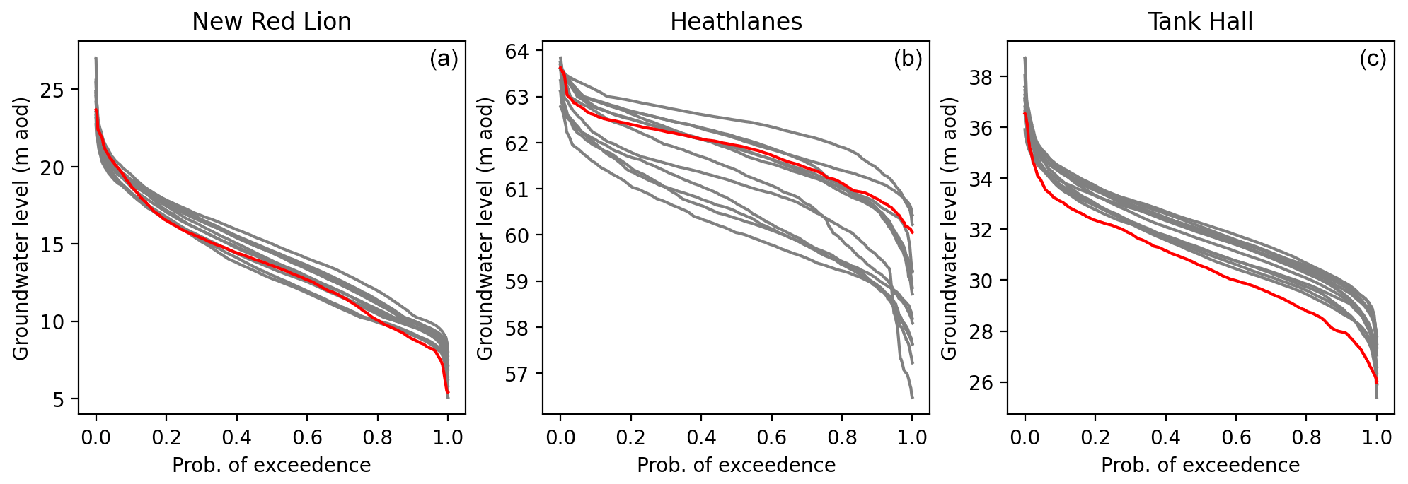
Figure 8 Groundwater level duration curves (GLDCs) for the period 1989–2018 using the simrcm (grey lines) and simobs (red line) simulations. GLDCs are featured for three boreholes in different hydrogeological settings which show contrasting behaviour: (a) New Red Lion (Lincolnshire Limestone), (b) Heathlanes (Permo-Triassic Sandstone, Shropshire) and (c) Tank Hall (Chalk).

7.3 Low river flows and groundwater levels

Replication of observed low river flows and groundwater levels over a baseline period provides an indication of how well the simrcm runs are performing in the lower part of the river flow and groundwater level regime and therefore enhances confidence in future low-flow and low-level projections. Figure 9a–d show the difference between the simobs and simrcm 90 % exceedance flow (Q90) over the 1989–2018 baseline period reported as the absolute percentage error (APE) at each of the 200 catchments for all four river flow models.

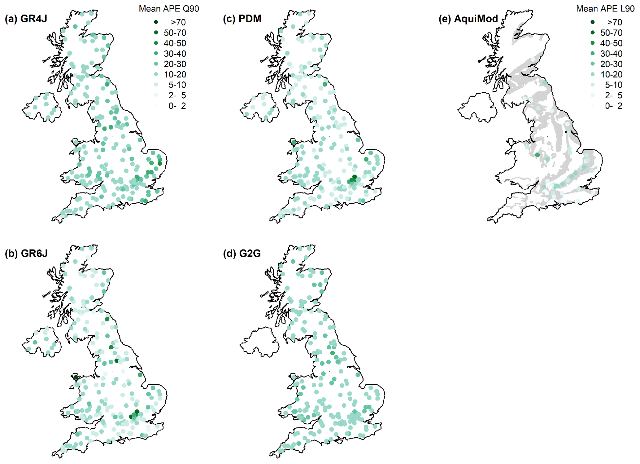
Figure 9 Comparison of simobs and simrcm runs for river flows and groundwater levels exceeding 90 % of the time (Q90 and L90 respectively) between 1989 and 2018. The colour scale indicates the mean of 12 absolute percent errors (APEs) between Q90 (L90) in model observations and Q90 (L90) in each of 12 ensemble members. Results are presented for (a) GR4J, (b) GR6J, (c) PDM, (d) G2G and (e) AquiMod. Note: AquiMod levels are expressed as a percentage of the simobs range in groundwater levels to remove the influence of aquifer storage. Figures S16 to S18 feature the equivalent baseline assessment for Q30 (L30), Q50 (L50) and Q70 (L70).

Overall, there is a reasonable agreement between the simobs and simrcm Q90 values across all four models. Mean APEs are less than 20 % for most catchments across the four hydrological models. Modelled low flows for GR6J, G2G and particularly PDM are especially well replicated in catchments across the UK, with mean APEs higher (20 %–50 %) in GR4J river flows for catchments in East Anglia and parts of northern England and southern Wales. The lumped catchment models GR6J and PDM struggle to capture low flows in groundwater-influenced catchments of the eastern Chilterns north of London, with APEs of up to 70 %. Considering the natural flows simulated by G2G and the prevalence of artificial influences on rivers further south and east in the UK, mean APEs are reasonable in this region and are actually higher in more natural parts of Wales and northern England.

Mean APEs at a range of other flow quantiles demonstrate similar patterns (Figs. S16 to S18). Mean APEs of Q30 for the vast majority of catchments for all four hydrological models are less than 20 % (Fig. S16). Mean APEs of Q50 (Fig. S17) and Q70 (Fig. S18) are also reasonable in most catchments and models, though higher mean APEs (20 %–50 %) are apparent for both of these flow quantiles in East Anglia for GR4J, in parts of northern England for G2G and in groundwater-influenced parts of the Chilterns for PDM. Mean APEs are similarly higher in GR6J flows at Q50 in East Anglia and at Q70 in the groundwater-influenced Chilterns. Whilst this analysis is primarily an assessment of the ability of the RCM ensemble to replicate flows across the regime, it is clear that the hydrological model calibrations also have a role in influencing the outcomes.

Figure 9e shows the difference between the simobs and simrcm 90 % exceedance groundwater level (L90) over the 1989–2018 baseline period reported as an APE relative to the simobs range in groundwater levels at each of the 54 boreholes. The use of the range in groundwater level as a reference removes the influence that the aquifer storage has on groundwater variability across the boreholes. There is good agreement between the simobs and simrcm L90 values across the boreholes. Mean APEs are less than 20 % for all of the boreholes except for the Heathlanes borehole in the Permo-Triassic Sandstone, where the mean APE exceeds 30 %.

Mean APEs at a range of other groundwater level quantiles demonstrate similar patterns (Figs. S16 to S18). Mean APEs of L30 do not exceed 5 % for the majority of the boreholes. The mean APEs typically become larger for most boreholes as the level quantile reduces towards L90. Heathlanes consistently has the highest mean APE for all level quantiles.

7.4 Seasonal groundwater recharge

Figure 10 provides a comparison of simobs and simrcm runs for seasonal-average groundwater recharge between 1989 and 2018 generated by ZOODRM. During the winter months (DJF), when groundwater recharge is highest, the simrcm simulations show good correspondence to simobs simulations, where the mean APE is less than 20 % for all but seven of the groundwater bodies. During the summer months (JJA), when groundwater recharge is lowest, the majority of the groundwater bodies still show mean APEs of less than 20 %, but over 200 of them show errors exceeding 20 %. These larger errors are typically associated with groundwater bodies that have lower-than-average recharge for this time of the year. For MAM, the majority of the groundwater bodies with errors that exceed 20 % are also associated with those groundwater bodies with below-average recharge for that time of the year. There are also some additional areas with significant recharge that show errors exceeding 20 %, including groundwater bodies in eastern–central Scotland and north-western and south-western England. For autumn (SON), the simrcm simulations show good correspondence to simobs simulations, where the majority (>80 %) of the groundwater bodies show mean APEs of less than 20 %. The majority of those with larger errors are situated on the eastern coast of Scotland and England and in northern Wales and Cheshire.

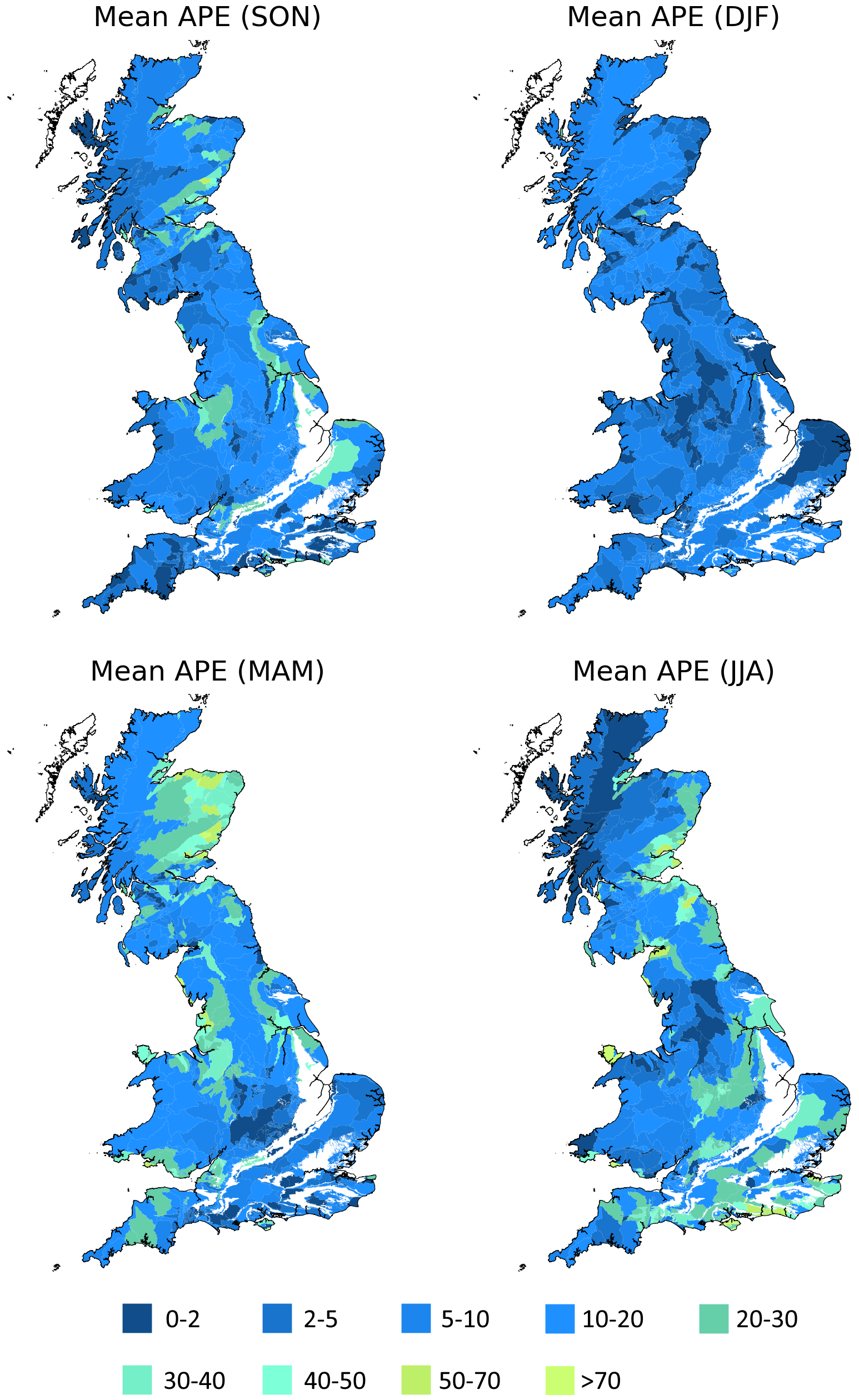
Figure 10 Comparison of simobs and simrcm runs for seasonal-average groundwater recharge between 1989 and 2018 generated by ZOODRM. The colour scale indicates the mean of 12 absolute percent errors (APEs) between simobs and simrcm.

Table 3 eFLaG dataset structure information.

8 Data availability

The eFLag dataset is associated with a digital object identifier. This must be referenced fully for every use of the eFLag data as https://doi.org/10.5285/1bb90673-ad37-4679-90b9-0126109639a9 (Hannaford et al., 2022).

All eFLaG files are available through the UKCEH EIDC: https://catalogue.ceh.ac.uk/documents/1bb90673-ad37-4679-90b9-0126109639a9 (last access: 29 March 2023, Hannaford et al., 2022).

The data are stored as .csv files in the folder structure shown in the guidance note available in Hannaford et al. (2022). In total, there are 3304 files, 1 for each variable, model and catchment–borehole combination. They can be broadly split into two groups of files (Table 3), simobs and simrcm, as follows.

• simobs. For the meteorological data, the simobs files contain date-indexed, observation-driven simulation (sim) data for precipitation with snowmelt and potential evaporation. For river flows and groundwater levels, the simobs files contain date-indexed, observation-driven simulations (sim) and associated observations (obs) if they exist.

• simrcm. For the meteorological data, the simrcm files contain date-indexed, RCM-driven simulations for the 12 RCMs used in eFLaG for precipitation with both snowmelt and potential evaporation. For river flows and groundwater levels, the simrcm files contain date-indexed, RCM-driven simulations for the 12 RCMs used in eFLaG, where modelname is G2G, PDM, GR4J and GR6J. NRFA station numbers and NGLA borehole names are given in the eFLaG_Station_Metadata.xlsx workbook.

• The gridded bias-corrected precipitation data are also made available as a separate dataset at the EIDC (Lane and Kay, 2022): https://doi.org/10.5285/755e0369-f8db-4550-aabe-3f9c9fbcb93d.

Conditions of use

The eFLaG dataset is available under a licensing condition agreement. For non-commercial use, the products are available free of charge. For commercial use, the data might be made available conditional on a fee to be agreed to with the UKCEH and NERC BGS licensing teams, owners of the IPRs (intellectual property rights) of the datasets and products.

9 Applications and limitations

9.1 Applications

The eFLaG dataset is presented as a nationally consistent dataset of future river flow, groundwater and groundwater recharge, using the latest available climate projections from UKCP18. In this article, we have described the dataset and its evaluation against observational hydrological datasets to give some confidence in the use of eFLaG as a dataset that can be used to assess the potential impacts on climate change in UK hydrology for a very wide range of applications.

The eFLaG dataset was developed specifically as a demonstration climate service for use by the water industry for water resources and drought planning and hence by design is focused on future projections of drought, low river flows and low groundwater levels. We therefore present eFLaG primarily as a dataset for this purpose. Ongoing work is underway to demonstrate the utility of eFLaG for future drought projections (Parry et al., 2023; Tanguy et al., 2023) and for future drought/water resources planning in practice (Counsell et al., 2023). The predecessor product, FFGWL, has been widely used within the water industry to provide insight into the future evolution of river flows and groundwater levels through the 21st century to support water resources management plans and also supported significant academic water resources planning studies (e.g. Borgeomo et al., 2015; Huskova et al., 2016).

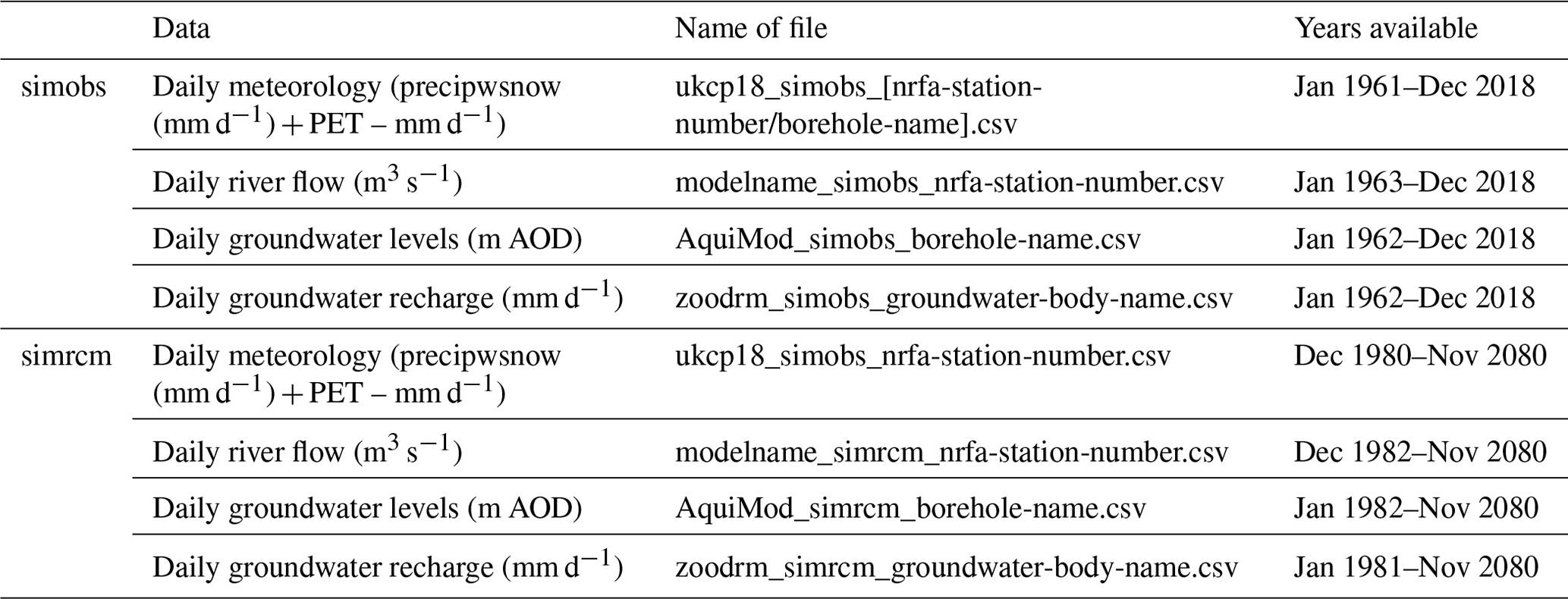
To provide users with a platform for accessing eFLaG datasets and all the evaluation approaches outlined here, an interactive web application has been developed, the eFLaG Portal (https://eip.ceh.ac.uk/hydrology/eflag/, last access: 29 March 2023). The portal provides a user-friendly front-end for accessing eFLaG results, with several examples shown in Fig. 11. The figure demonstrates how eFLaG data can be used to project future drought characteristics for various time slices and also how low-flow characteristics change through the 21st century, based on the analysis conducted in Parry et al. (2023).

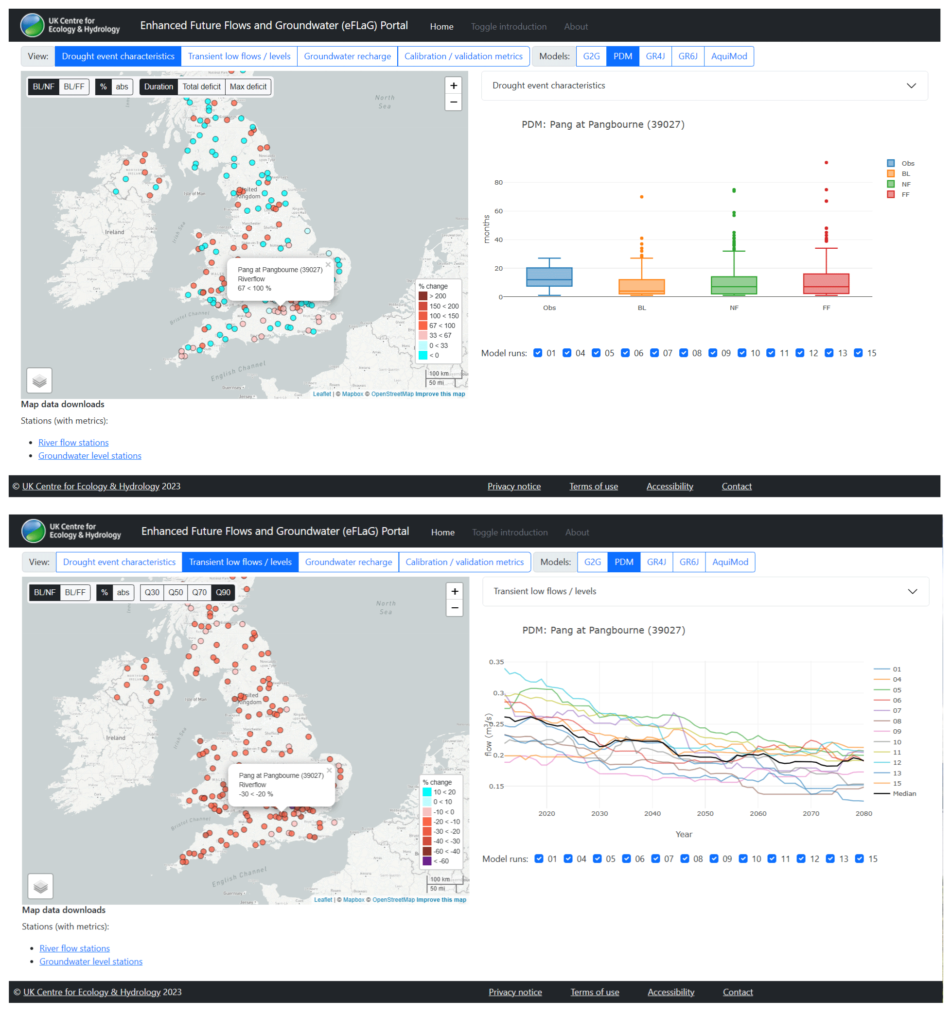
Figure 11 Screenshots from the eFLaG Portal. Top: map showing percentage change in drought duration between baseline and near future for eFLaG catchments nationally, using PDM; box plots showing percentage changes (using PDM) for a river in southern England (the river Pang) for three time slices, with box plots showing range of RCM uncertainty; other drought characteristics available on other tabs. Bottom: map showing percentage change in a low flow metric (Q90) between baseline and near-future for eFLaG catchments nationally, using PDM; with time series showing transient projections of Q90 in moving windows through to the 2080s for the river Pang, each colour representing different RCM runs, black representing median. For all outputs, models other than PDM can be selected using the tabs at the top.

By providing a consistent dataset of future river flows, groundwater levels and groundwater recharge, eFLaG can potentially support a wide range of applications across other sectors. The FFGWL product also found very wide application for diverse research purposes (for water quality, e.g. Charlton et al., 2017, hydroecology, e.g. Royan et al., 2015, groundwater recharge, Hughes et al., 2021, or groundwater level reconstruction, Jackson et al., 2016). For eFLaG, the good simulation of river flows and groundwater behaviours across much of the hydrological range suggests that this product could also find application in a whole range of impact studies, subject to additional evaluation for the purposes in mind. While not validated specifically for floods, the encouraging evaluation outputs for higher-flow percentiles suggests users can analyse high-flow metrics and variability (e.g. frequency of flows above a threshold), even if not annual maximum peak flows.

As with FFGWL, there are a number of advantages of using eFLaG for future projections: it is a spatially coherent dataset, meaning that future changes in hydrological variables can be compared between catchments, boreholes and aquifers at the regional to national scales. This is a key benefit for both research and practical water resources planning. Spatially coherent projections are needed to address the spatio-temporal dynamics of droughts (e.g. Tanguy et al., 2021), how these may change in the future and what this may mean for water resources planning – where, in practice, water resources management plans often involve transfers between regions (e.g. Murgatroyd et al., 2021). Tanguy et al. (2023) address the changing future spatial coherence of droughts using eFLaG.

Another key benefit of eFLaG is that transient time series (daily data from 1980 to 2080) allow users to explore the future evolution of river flow and groundwater variability on interannual and decadal timescales rather than just using change-factor approaches that compare between future time slices and the baseline.

The use of an ensemble of outputs enables users to consider uncertainty in driving data (via the 12-member RCM ensemble) as well as, for river flows, hydrological model uncertainty. In addition, different models provide different benefits: G2G performs less well against observations than the (calibrated) lumped catchment models but does enable the characterisation of natural flows, which is vital for some uses (e.g. in providing naturalised river flows for regionalisation or as a baseline for assessing impacts, as is common in regulatory and hydroecology applications, e.g. Terrier et al., 2021). Moreover, abstractions and discharges can be added to the naturalised runs, as demonstrated by Rameshwaran et al. (2022). This opens up the possibility of projecting the evolution of future naturalised and impacted river flows separately – a follow-up study on this topic is underway by the authors.

Furthermore, G2G's response to rainfall may be less tailored to the present-day climate than the calibrated models, as noted in the limitations section. The eFLaG hydrological model ensemble therefore includes models that may be beneficial for different applications according to the particular needs of end-users.

9.2 Limitations and guidance

Users of the eFLaG dataset should be aware of its limitations. While the evaluation shows encouraging results at the national scale, there are inevitably some catchments and boreholes where the evaluation (either Stage 1, Stage 2 or both) indicates poorer-quality simulations. Users must be aware of this and should consult all the provided evaluation metrics when considering which catchments to use (and which models to use) in their analyses.

Users must also be aware that, while there is some consideration of uncertainty through the adoption of the RCM PPE and the use of multiple models for river flows, there are many other sources of uncertainty not sampled in eFLaG. While the PPE gives a range of 12 outcomes, it is only one UKCP18 product and one emissions scenario and so does not sample the full range of outcomes in UKCP18. The emissions scenario, RCP8.5, is considered to be a pessimistic scenario (Hausfather and Peters, 2020), so this should be borne in mind, and the eFLaG projections (along with other uses of the UKCP18 regional projections) can arguably be seen as akin to a “worst case” for planning (Arnell et al., 2021). Future work should position eFLaG against the wider range of UKCP18 outcomes. Furthermore, only one bias-correction approach is used.

Although we use a range of river flow models, clearly other hydrological models could provide different outcomes than the set used here, and we have only used one groundwater level model and recharge model respectively and so have not considered model uncertainty for groundwater. We have also not considered other sources of uncertainty in the hydrological modelling (e.g. parametric uncertainty, as in e.g. Smith et al., 2019) or the impacts of different observational driving climate datasets (e.g. different formulations of potential evapotranspiration, as in e.g. Tanguy et al., 2018). These studies demonstrate that these can be significant sources of uncertainty, but it was beyond our scope to consider them within the time and resources constraints of eFLaG given the high number of existing runs that were necessary. Future studies should address these further sources of uncertainty.

The eFLaG modelling framework adopted the approach of calibrating using a full period of record rather than using a split-sample approach. Given the length of the record, this is unlikely to be too significant (as shown for GR4J in the UK by Harrigan et al., 2018b) relative to using split-sampling, but at the same time, uncertainties inevitably remain about future projections well outside the calibration period, not least given likely non-stationarities in catchment properties. It should also be borne in mind that a strong performance of a model as indicated by good metric values is not necessarily a reliable indicator of a model's ability to reproduce trends in hydrological signatures such as those describing low flows (Todorović et al., 2022) – this is particularly the case for the future under a changing climate.

Following on from this, one important limitation of this study – in common with the original Future Flows product (Prudhomme et al., 2012) and indeed a great majority of climate projections in hydrology – is the lack of explicit modelling of human disturbances. This is simply unavoidable, as large-scale datasets of artificial influences have only recently been made available in the UK, and only for England (e.g. Rameshwaran et al., 2022). This especially applies to the lumped catchment models and the groundwater level model. As such processes are not represented, they will simply be accounted for implicitly during calibration. Of course, this is unrealistic, as artificial influences are likely to change in the future and such non-stationarity could be locally significant. However, it should be borne in mind that the purpose of eFLaG is to model future river flow characteristics based on current catchment conditions rather than to truly chart future river flow trajectories in these catchments. For most practical applications, assuming current artificial influences and projecting forwards in time is entirely reasonable, especially in the absence of any informed understanding of how artificial influences will change.

There are also considerations for end-users when applying the projections directly in impact assessments. Notably, the HadREM3-GA705 climate model that underpins the UKCP18 RCM outputs is run on a 360 d calendar year. The eFLaG projections do not modify this calendar when producing the meteorological, hydrological and hydrogeological variables, and it is therefore the responsibility of the end-user to deal with this in an appropriate way. There are a number of ways of doing this (e.g. Prudhomme et al., 2012; Dobor et al., 2015), and, in general, there is no agreed-upon optimal approach. Where this is performed as a post-processing step by the user (as with the eFLaG datasets), it is likely that the best approach will depend on the impact or system modelling being undertaken.

Finally, eFLaG only provides projections for a sub-set of the UK gauging station network (200 catchments from some 1200 in the NRFA). This is an inevitable constraint, as with the original FFGWL product (300 locations). While we have tried to sample UK hydrology to give users as much scope as possible, there will still be a need to transpose projections to sites of interest for some users. One of the benefits of eFLaG is that gridded river flow and recharge models are used. While these gridded datasets are not yet openly available, current follow-up initiatives are looking to exploit them to provide projections at ungauged locations. A gridded dataset using G2G, but with different driving data, is described by Kay et al. (2023).