the Creative Commons Attribution 4.0 License.
the Creative Commons Attribution 4.0 License.
 | 23 May 2023
Generation of global 1 km daily soil moisture product from 2000 to 2020 using ensemble learning
Yufang Zhang
Qian Wang
Bing Li
Jianglei Xu
Guodong Zhang
Xiaobang Liu
Changhao Xiong
Motivated by the lack of long-term global soil moisture products with both high spatial and temporal resolutions, a global 1 km daily spatiotemporally continuous soil moisture product (GLASS SM) was generated from 2000 to 2020 using an ensemble learning model (eXtreme Gradient Boosting – XGBoost). The model was developed by integrating multiple datasets, including albedo, land surface temperature, and leaf area index products from the Global Land Surface Satellite (GLASS) product suite, as well as the European reanalysis (ERA5-Land) soil moisture product, in situ soil moisture dataset from the International Soil Moisture Network (ISMN), and auxiliary datasets (Multi-Error-Removed Improved-Terrain (MERIT) DEM and Global gridded soil information (SoilGrids)). Given the relatively large-scale differences between point-scale in situ measurements and other datasets, the triple collocation (TC) method was adopted to select the representative soil moisture stations and their measurements for creating the training samples. To fully evaluate the model performance, three validation strategies were explored: random, site independent, and year independent. Results showed that although the XGBoost model achieved the highest accuracy on the random test samples, it was clearly a result of model overfitting. Meanwhile, training the model with representative stations selected by the TC method could considerably improve its performance for site- or year-independent test samples. The overall validation accuracy of the model trained using representative stations on the site-independent test samples, which was least likely to be overfitted, was a correlation coefficient (R) of 0.715 and root mean square error (RMSE) of 0.079 m3 m−3. Moreover, compared to the model developed without station filtering, the validation accuracies of the model trained with representative stations improved significantly for most stations, with the median R and unbiased RMSE (ubRMSE) of the model for each station increasing from 0.64 to 0.74 and decreasing from 0.055 to 0.052 m3 m−3, respectively. Further validation of the GLASS SM product across four independent soil moisture networks revealed its ability to capture the temporal dynamics of measured soil moisture (R=0.69–0.89; ubRMSE = 0.033–0.048 m3 m−3). Lastly, the intercomparison between the GLASS SM product and two global microwave soil moisture datasets – the 1 km Soil Moisture Active Passive/Sentinel-1 L2 Radiometer/Radar soil moisture product and the European Space Agency Climate Change Initiative combined soil moisture product at 0.25∘ – indicated that the derived product maintained a more complete spatial coverage and exhibited high spatiotemporal consistency with those two soil moisture products. The annual average GLASS SM dataset from 2000 to 2020 can be freely downloaded from https://doi.org/10.5281/zenodo.7172664 (Zhang et al., 2022a), and the complete product at daily scale is available at http://glass.umd.edu/soil_moisture/ (last access: 12 May 2023).
- Article
(14951 KB) - Full-text XML
- BibTeX
- EndNote


Soil moisture typically refers to the water content of the unsaturated soil zone (Liang and Wang, 2020). As an essential climate variable specified by the Global Climate Observing System, it plays a critical role in terrestrial water, energy, and carbon cycles (Dorigo et al., 2017; Humphrey et al., 2021). Over recent decades, soil moisture datasets have been used across a wide range of earth system applications, including climate-related research (Berg and Sheffield, 2018), hydrological modeling (Brocca et al., 2017), rainfall estimating (Brocca et al., 2019), disaster forecasting (Kim et al., 2019), and agriculture and ecosystem monitoring (Liu et al., 2020; Holzman et al., 2014), mainly attributed to the progress in remotely sensed soil moisture algorithms. However, substantial gaps remain between the currently released soil moisture products and the growing requirements of various applications, especially at regional and local scales (Peng et al., 2021).
Global soil moisture products can generally be obtained through model simulations or remote sensing, mostly at spatial resolutions of tens of kilometers. The advantages of simulated or reanalysis soil moisture datasets, such as the land component of the European ReAnalysis V5 (ERA5-Land) and the Global Land Data Assimilation System (GLDAS) soil moisture products (Rodell et al., 2004; Muñoz-Sabater et al., 2021), are their spatiotemporal continuity and availability of root-zone estimates; however, their corresponding errors can be rather large when the quality of forcing datasets or model performance are relatively poor (Sheffield et al., 2004). Alternatively, microwave remote sensing has been regarded as the most promising technique to acquire surface soil moisture estimates at global scale, due to its high sensitivity to soil water content dynamics and its capacity for all-weather monitoring (Babaeian et al., 2019; Shi et al., 2019). Currently, several global soil moisture products have been operationally generated from microwave scatterometers and radiometers, including the Advanced Scatterometer (ASCAT) and Advanced Microwave Scanning Radiometer for Earth Observing System (AMSR-E), in addition to instruments aboard the Soil Moisture and Ocean Salinity (SMOS) and Soil Moisture Active Passive (SMAP) satellites (Chan et al., 2016; Wagner et al., 2013; Njoku et al., 2003; Kerr et al., 2016), typically with a grid spacing of 9–50 km and a revisit cycle of 1–3 d.
Motivated by the lack of high spatial resolution soil moisture products that are capable of benefiting numerous regional-scale applications (Peng et al., 2021), various algorithms have been proposed to downscale the coarser global soil moisture products mentioned above (Peng et al., 2017), and some of which have been used to derive global or regional soil moisture products at fine scales in recent years. For example, by combing a Sentinel-1 synthetic aperture radar (SAR) dataset with the SMAP radiometer dataset, Das et al. (2019) generated global soil moisture products at 3 and 1 km resolutions. Song et al. (2022) downscaled the AMSR-E/AMSR-2 soil moisture products using optical reflectance from the Moderate Resolution Imaging Spectroradiometer (MODIS) and gap-filled land surface temperature (LST) datasets, producing a 1 km daily soil moisture product over China under all-weather conditions. Elsewhere, Naz et al. (2020) generated a daily soil moisture reanalysis dataset (ESSMRA) at 3 km resolution over Europe by assimilating the European Space Agency (ESA) Climate Change Initiative (CCI) product into a community land model via an ensemble Kalman filter method. Additionally, Vergopolan et al. (2021) recently released a 30 m subdaily soil moisture dataset across the conterminous United States (CONUS), which was retrieved using the merged 30 m brightness temperatures obtained by combining a hyper-resolution land surface model (HydroBlocks), a radiative transfer model, and the SMAP Enhanced Level 3 brightness temperatures at 9 km. Apart from these downscaled high-resolution datasets, several studies have directly derived the 1 km operational soil moisture products over Europe from multitemporal Sentinel-1 SAR images using change detection algorithms, showing potential for global coverage (Balenzano et al., 2021; Bauer-Marschallinger et al., 2019).
Table 1 lists the spatial and temporal coverages, temporal resolution, and grid spacing (i.e., pixel size, which may be finer than the actual spatial resolution) of several representative and publicly available soil moisture products. Accordingly, there remains a lack of long-term global soil moisture products at both high spatial and temporal resolutions. Although the SMAP/Sentinel-1 L2 Radiometer/Radar soil moisture dataset (SPL2SMAP_S) has global coverage and a spatial resolution up to 1 km, its temporal resolution degrades to 12 d over most regions, owing to the relatively long revisit cycle of Sentinel-1 SAR satellites. Recently, Zheng et al. (2023) developed a global seamless soil moisture dataset by downscaling the 0.25∘ ESA CCI product using a random forest model, achieving an R of 0.89 and unbiased RMSE (ubRMSE) of 0.045 m3 m−3, but they only adopted a random cross-validation strategy which is likely to be affected by model overfitting. Other downscaled soil moisture datasets generally maintain regional or continental coverage, limited by the lack of high-resolution seamless input datasets or model applicability. Optical and thermal remote sensing techniques can provide long-term observations with high spatiotemporal resolutions, which have been widely used to derive soil moisture or relevant indices (Yue et al., 2019; Ghulam et al., 2007; Rahimzadeh-Bajgiran et al., 2013). However, optical and thermal satellite datasets can be detrimentally affected by cloud coverage, hindering their use in soil moisture retrieval or downscaling across a global scale. To address this issue, the latest versions of the Global Land Surface Satellite (GLASS) products (Liang et al., 2021) were used here, including the spatiotemporally continuous surface albedo, leaf area index (LAI), and land surface temperature (LST), which were produced with reliable accuracies primarily based on MODIS observations. In the present study, these fine-scale GLASS products were integrated with auxiliary datasets (terrain and soil texture) and the seamless ERA5-Land reanalysis soil moisture product at a coarse scale using an ensemble machine learning model to estimate daily soil moisture at 1 km resolution. This framework was adapted from Zhang et al. (2022b), where models were trained using Landsat 8 observations and multisource datasets as inputs, and with the International Soil Moisture Network (ISMN) measurements as the target. To produce a seamless global soil moisture product, Landsat datasets prone to cloud interference were replaced with spatiotemporally continuous GLASS products. Considering the large-scale difference between GLASS products and in situ soil moisture compared to Landsat datasets, the triple collocation (TC) technique (Stoffelen, 1998; McColl et al., 2014) was adopted to select the representative soil moisture stations prior to model training for mitigating the influence of scale mismatch on prediction accuracy.
Specifically, the aim of this research was to provide a long-term (2000–2020) global soil moisture dataset (GLASS SM) with high spatiotemporal resolutions (1 km, daily) and reliable accuracy. To achieve this goal, an ensemble learning model, eXtreme Gradient Boosting (XGBoost) (Friedman, 2001; Chen and Guestrin, 2016), was developed by integrating multisource datasets. The model was then applied to generate the global 1 km GLASS SM product, which was further evaluated against four independent soil moisture networks. Lastly, an intercomparison was made between the derived product and two global microwave soil moisture products to investigate their spatiotemporal consistency.
Table 1Main characteristics of several representative and publicly available soil moisture products.
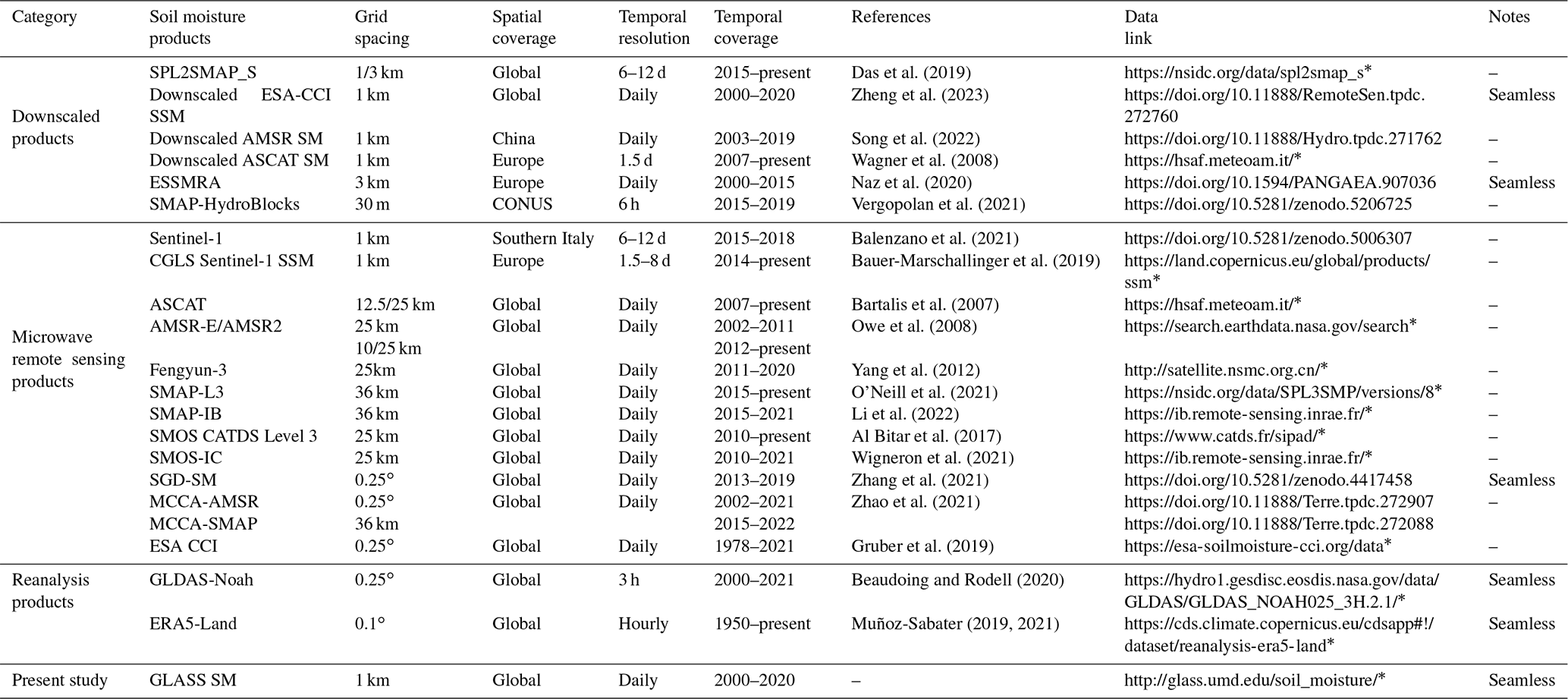
* Last access: 12 May 2023. SSM represents surface soil moisture. CGLS represents the Copernicus Global Land Service.
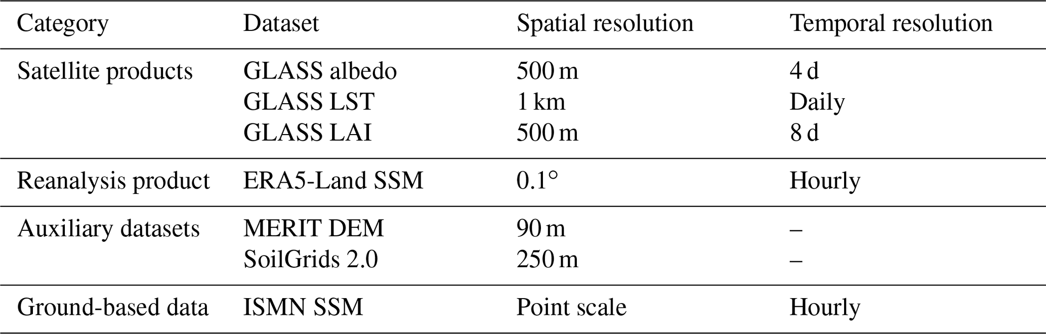
The multisource datasets used to generate the global high-resolution soil moisture product here can be grouped into four categories (Table 2). Namely, remotely sensed variables derived from the three GLASS products, reanalysis surface soil moisture from the ERA5-Land dataset, and auxiliary variables extracted from the Multi-Error-Removed Improved-Terrain (MERIT) DEM and SoilGrids products were used to train an XGBoost model for estimating the global soil moisture product, whereas globally distributed in situ soil moisture measurements from ISMN stations were used as targets for model training. In addition, four independent in situ soil moisture datasets and two microwave soil moisture products were used to validate and compare the derived global product.
Table 2Multisource datasets used to generate the global high-resolution soil moisture product.
2.1 Remotely sensed datasets
The GLASS product suite has been employed in various applications owing to its long-term coverage, spatial continuity, high spatial resolution, and accuracy (Liang et al., 2021). Here, the latest version of GLASS albedo, LST, and LAI products served as the primary inputs to the ensemble learning model. Specifically, the GLASS V6 LAI product (500 m resolution) was generated from six MODIS 8 d surface reflectance bands of MOD09A1 using a bidirectional long short-term memory deep learning model (http://www.glass.umd.edu, last access: 12 May 2023) (Ma and Liang, 2022). Notably, this product is relatively more accurate than the 250 m GLASS LAI estimated from two bands of MOD09Q1. The all-sky 1 km GLASS LST was produced by integrating multiple datasets from MODIS, reanalysis, and in situ LST measurements using a random forest model (Li et al., 2021). Daily global LSTs averaged from instantaneous GLASS LST products were used here, which will be also released at http://www.glass.umd.edu. The gap-free GLASS albedo products were generated using a combination of a direct-estimation algorithm (Qu et al., 2014) and a spatiotemporal filtering scheme (Liu et al., 2013). Namely, the black-sky visible, near-infrared, and shortwave albedo data extracted from the GLASS V42 albedo products were used in the present study (http://www.glass.umd.edu).
2.2 ERA5-Land reanalysis soil moisture product
ERA5 provides a range of global atmospheric, terrestrial, and oceanic variables from 1950 to present at 31 km spatial resolution (Hersbach et al., 2020). Specifically, ERA5-Land is an enhanced global land reanalysis dataset obtained by downscaling the atmospheric forcing derived from the reanalysis of ERA5 to a native resolution of approximately 9 km (Muñoz-Sabater et al., 2021). ERA5-Land includes hourly estimates of volumetric soil moisture at four soil layers and a grid spacing of 0.1∘ (https://cds.climate.copernicus.eu/, last access: 12 May 2023). In the present study, the top layer (0–7 cm) ERA5-Land soil moisture were used to match the shallow observation depths of optical satellites. The daily average soil moisture was calculated and resampled to 1 km before being used as an input variable of the ensemble learning model.
2.3 Static terrain and soil texture datasets
Topography and soil properties, which can be treated as static variables due to their relatively slow rate of change over the short term, have an important influence on the spatial variations of soil moisture at finer scales. The global terrain dataset used in the study here was the high-accuracy MERIT DEM with a spatial resolution of 3 arcsec (∼ 90 m at the Equator). The MERIT DEM integrates several spaceborne DEMs after eliminating their inherent primary error components, including speckle noise, stripe noise, absolute bias, and tree height bias (http://hydro.iis.u-tokyo.ac.jp/~yamadai/MERIT_DEM/, last access: 12 May 2023) (Yamazaki et al., 2017). After deriving the elevation, aspect, and slope from the MERIT DEM, these topographic variables were resampled to 1 km and used as input features for the model. Alternatively, soil texture was derived from the SoilGrids V2.0 product at 250 m resolution (https://www.isric.org/explore/soilgrids, last access: 12 May 2023). SoilGrids uses > 240 000 soil profile measurements and > 400 environmental covariates worldwide to train machine learning models and produce global soil property maps across six depth intervals (Poggio et al., 2021). Recent studies have shown that the SoilGrids product has both higher resolution and enhanced accuracy compared to other soil datasets at the global scale (Dai et al., 2019), in addition to the ability of soil texture data to improve the bias and root mean square error (RMSE) of downscaled soil moisture products (Das et al., 2019). Accordingly, the mean contents of sand, silt, and clay were extracted for the first soil layer (0–5 cm) from the SoilGrids database and resampled to 1 km.
2.4 Ground-based soil moisture training dataset
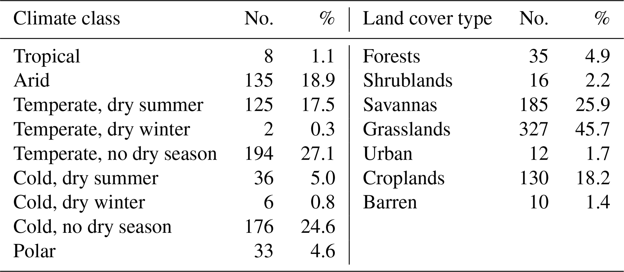
The ISMN aims to establish and maintain a global database of in situ soil moisture measurements for the validation and improvement of satellite-based and modeled soil moisture products. Currently, it consists of 73 networks with over 2800 soil moisture stations worldwide, providing quality-controlled and harmonized datasets collected from monitoring networks and field experiments (Dorigo et al., 2021). Here, data for the period from 2000–2018 were obtained (https://ismn.earth/, last access: 12 May 2023), and only stations with a sensing depth of < 5 cm were selected to match the observation depth of remotely sensed datasets. Soil moisture records were then screened according to the quality flags provided with the ISMN dataset (Dorigo et al., 2013), before being used as the training target for the machine learning model. The spatial distribution of the representative ISMN soil moisture stations selected using the TC method described in Sect. 3.2 is displayed in Fig. 1. The number and percentage of representative stations for each land cover type and climate class, which are calculated by using the 500 m MODIS land cover type product (Friedl and Sulla-Menashe, 2019) and the 1 km Köppen–Geiger climate classification dataset (Cui et al., 2021), respectively, are also shown in Table 3.
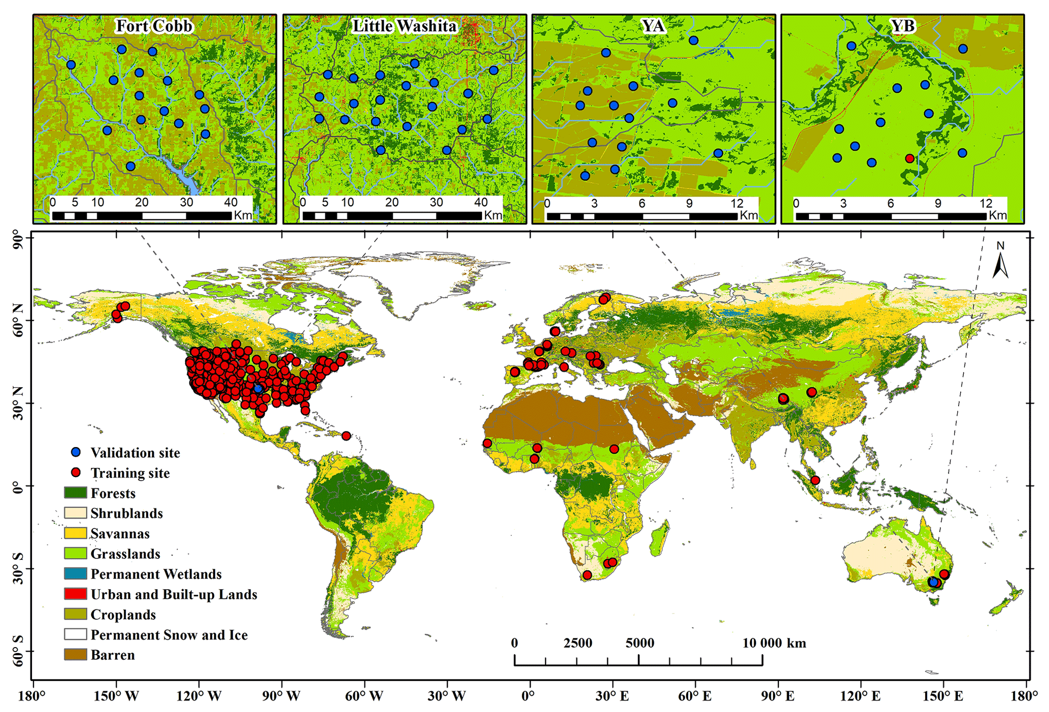
Figure 1Spatial distribution of the 715 representative ISMN soil moisture stations used for training the model and four independent soil moisture networks used for validation, with the MODIS land cover type product (MCD12Q1) for 2016 displayed in the background.
Table 3The number and percentage of representative ISMN soil moisture stations for each climate class and land cover type.
2.5 Independent in situ validation datasets
Four soil moisture monitoring networks that were not included in the ISMN database were used to assess the model's ability to capture temporal variations in soil moisture over unknown area (Fig. 1). The YA and YB subnetworks are both part of the Yanco soil moisture network, located in a semiarid agricultural region of the Murrumbidgee River basin, Australia, with a flat topography and elevation spanning 117–150 m (Yee et al., 2017). There are 13 and 11 stations in the YA and YB subnetworks, respectively, distributed across two 9 × 9 km areas, and soil moisture observations from these stations can be downloaded from the Oznet Hydrological Monitoring website (http://www.oznet.org.au, last access: 12 May 2023) (Smith et al., 2012). Two other micronets (Fort Cobb and Little Washita) are located in southwestern Oklahoma, USA, and are characterized by a humid subtropical climate (Starks et al., 2014). The primary land cover types are cropland and rangeland, and the topography is moderately rolling (Bindlish et al., 2009). Currently, there are 15 and 20 operational stations in the Fort Cobb and Little Washita networks, respectively, for which soil moisture datasets can be accessed through the Grazinglands Research Laboratory (https://ars.mesonet.org/, last access: 12 May 2023). These four dense soil moisture networks have been used extensively to either validate or calibrate satellite soil moisture products (Ma et al., 2021; Colliander et al., 2017; Chan et al., 2018).
2.6 Microwave soil moisture product
To further validate the spatiotemporal performance of the derived 1 km soil moisture product here, two additional microwave-based products were selected for comparison. The first product is the high-resolution SMAP/Sentinel-1 SPL2SMAP_S dataset, which contains the first global 1 km soil moisture product that was publicly released in the past (Table 1). It has a temporal resolution of 6–12 d and can be downloaded from the National Snow and Ice Data Center at 1 and 3 km resolutions (https://nsidc.org/data/spl2smap_s, last access: 12 May 2023). According to Das et al. (2019), the average unbiased RMSE (ubRMSE) values achieved by both the 1 and 3 km SPL2SMAP_S products over sparse soil moisture networks were approximately 0.05 m3 m−3. Considering that the SPL2SMAP_S baseline algorithm generally shows higher validation accuracy than the optional algorithm (directly disaggregating the SMAP 9 km soil moisture product) and that the AM (descending orbit combination) soil moisture retrievals are more accurate than their APM (a.m. or p.m.) equivalents (descending or ascending orbits combination) (Xu, 2020), the baseline AM soil moisture field “disagg_soil_moisture_1km” data were extracted from the SPL2SMAP_S 1 km data group and used for comparison. The second product is the CCI global soil moisture dataset released by the ESA, with a grid spacing of 0.25∘ and daily temporal resolution, which combines various passive and active microwave soil moisture products into a harmonized record with improved spatiotemporal coverages and has been fully validated across numerous global applications (Gruber et al., 2019; Dorigo et al., 2017). Specifically, the combined (active and passive) soil moisture product from CCI V6.1 was used here (https://esa-soilmoisture-cci.org/data, last access: 12 May 2023).
3.1 Overall framework
Soil moisture is characterized by high spatiotemporal variability, and its distribution is influenced by a range of environmental factors across different scales, such as climate, geographical conditions, soil properties, and surface coverage (Crow et al., 2012; Luo et al., 2022). Here, high-accuracy, spatiotemporally continuous GLASS products, including LST, albedo, and LAI, were used to provide surface temperature, spectral information on soil and vegetation, and information related to vegetation type and density. Considering the impact of topography and soil properties on soil moisture, topographic and soil texture fraction variables were extracted from the MERIT DEM and SoilGrids products, respectively. Additionally, the 0.1∘ ERA5-Land reanalysis soil moisture product was used to provide background soil moisture information. By utilizing an ensemble machine learning model, various variables extracted from these multisource datasets were integrated so that different environmental factors affecting soil moisture could be accounted for, and then soil moisture at fine scales could be estimated.
Figure 2 shows a flowchart of the proposed 1 km, spatiotemporally continuous soil moisture estimation framework. Prior to the training phase, the TC method and the other two long-term soil moisture datasets (ERA5-Land reanalysis and ESA CCI soil moisture products) were adopted for selecting the representative soil moisture stations, considering the scale difference between point-scale soil moisture measurements collected by ISMN stations and GLASS products (the detailed selection procedure is presented in Sect. 3.2). Then, multiple variables were extracted from the corresponding input datasets and spatiotemporally collocated with the in situ soil moisture measurements from the representative stations between 2000 and 2018. Specifically. the black-sky visible, near-infrared, shortwave albedo, LAI, and LST were extracted from the three GLASS products, based on the geographic locations of stations. Each of these variables, together with topographic and soil texture fraction variables, and the coarse-scale reanalysis soil moisture were put into the XGBoost model, which was chosen to simulate the nonlinear relationship between multiple input features and in situ soil moisture (the target variable). Lastly, those multisource input datasets were resampled to 1 km and then put into the developed XGBoost model for predicting the global 1 km spatiotemporally continuous soil moisture product (GLASS SM). Moreover, the GLASS SM product was evaluated against four independent soil moisture datasets and then compared the SPL2SMAP_S and CCI soil moisture products for spatiotemporal consistency analyses.
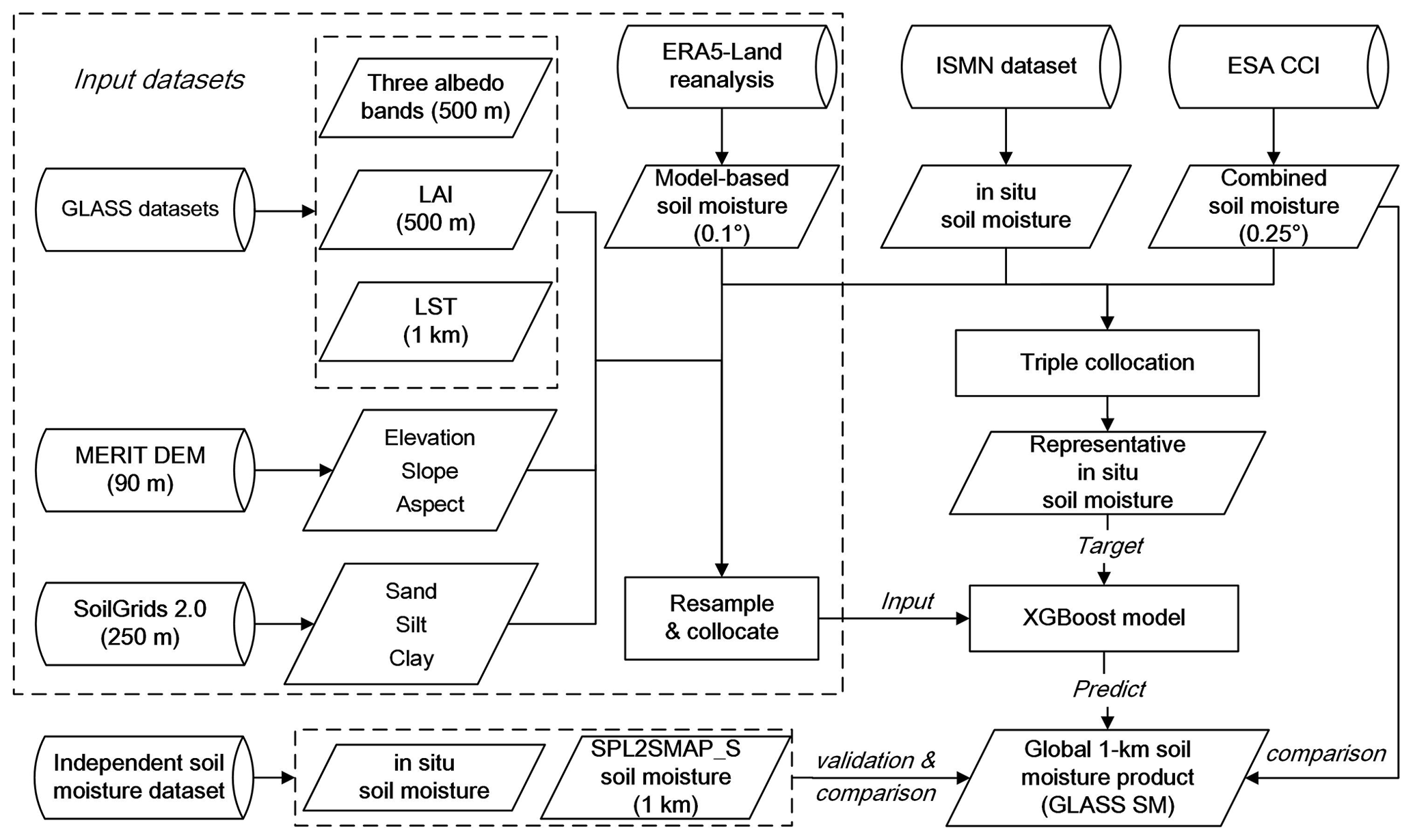
Figure 2Flowchart of the proposed 1 km spatiotemporally continuous soil moisture estimation framework.
3.2 Triple-collocation-based station selection
As mentioned above, in situ soil moisture data from the ISMN stations were employed as the target variable to train the XGBoost model, which was then used to predict soil moisture product at 1 km resolution. The underlying assumption was that the measured soil moisture at these point-scale stations is representative of the average moisture status of the corresponding 1 km pixel; however, because of the high spatiotemporal variability of soil moisture, this assumption is not always upheld. Accordingly, the TC method, which has been widely applied to analyze the coarse-scale spatial representativeness of in situ soil moisture dataset (Gruber et al., 2013; Molero et al., 2018), was adopted here to select the most representative stations. Specifically, TC is an error analysis method proposed by Stoffelen (1998) employing three collocated datasets to address large uncertainties in wind speed measurements. TC has also been widely used in the evaluation of satellite soil moisture products given the limited number of core validation sites at the satellite footprint scale (Zheng et al., 2022). The commonly used error model for TC analysis is defined in Eq. (1):
where Xi refers to the three collocated soil moisture observations; θ refers to the unknown true value of soil moisture; αi and βi are the additive and multiplicative biases of Xi relative to the true value, respectively; and εi is the random additive noise with zero mean. The assumptions underlying this error model and detailed derivation process for the error variance of each dataset can be found in Gruber et al. (2016). Notably, the assumptions made for TC analysis are similar to those made for the correlation coefficient (R) and RMSE (Gruber et al., 2016). To fulfill the independent error requirement of the TC analysis across the three datasets, the ISMN in situ soil moisture, model-based ERA5-Land soil moisture, and CCI combined microwave soil moisture were selected to construct the triplet. Among them, the CCI soil moisture product was selected here rather than other microwave soil moisture products, as it maintains a sufficiently long timescale to cover that of the training samples. The error variance of the ISMN soil moisture dataset, , was then calculated according to Eq. (2):
where is the variance of the ISMN in situ soil moisture; Cov is the covariance operator; and Xismn, Xera, and Xcci denote the collocated ISMN, ERA5-Land, and CCI soil moisture observations, respectively. Based on TC analysis, McColl et al. (2014) proposed a method called extended triple collocation (ETC) to estimate the correlation coefficient between each dataset and the unknown target variable. Specifically, the ETC correlation coefficient of the ISMN soil moisture dataset, RETC, can be calculated via Eq. (3):
where the sign of RETC was corrected to positive. It is a scaled, unbiased signal-to-noise-ratio metric complementary to . Using the above TC-based metrics and referring to previous studies (Yuan et al., 2020; Anderson et al., 2012), several strict conditions were established to select the most representative ISMN stations: (1) > 500 triplets were available at the station during the period 2000–2018, (2) the R between any two soil moisture datasets in the triplets was > 0.2, (3) the square root of the calculated for the ISMN soil moisture dataset was < 0.06 m3 m−3, and (4) the RETC between the ISMN soil moisture and the unknown soil moisture true values was > 0.7. A total of 715 representative ISMN soil moisture stations were finally selected, as shown in Fig. 1.
3.3 XGBoost model
Ensemble machine learning models can be roughly classified into two categories based on how the individual learners are generated: bagging and boosting (Zhou, 2021). For bagging models, the individual learners are constructed independently; whereas for boosting models, learners are constructed iteratively, increasing the weights for the incorrectly classified samples during each round of training. As a representative bagging algorithm, random forest has gained considerable attention in the fields of remote sensing classification and regression over recent decades (Belgiu and Drãguþ, 2016); however, it may suffer from a large prediction bias, especially when the observations are too large or small (Song, 2015). In contrast, boosting models have been shown to reduce both variance and bias and are robust to multicollinearity among predictors (Gislason et al., 2006; Karthikeyan and Mishra, 2021). Accordingly, the present study employed the XGBoost model implemented by Chen and Guestrin (2016) based on a gradient boosting framework (Friedman, 2001). The XGBoost model is advantageous for its scalability, efficiency, and decreased vulnerability to overfitting. Here, the open-source xgboost and Scikit-learn Python packages were used together for model training and hyperparameters tuning, with the grid search method being adopted to determine the optimal parameters. Here, the key hyperparameters of the XGBoost models were finally set to n_estimators (the number of the boosting rounds) = 1000, learning_rate = 0.1, and max_depth (maximum tree depth) = 8.
3.4 Evaluation strategies and performance metrics
While most previous soil moisture estimation studies based on machine learning have only used the random validation approach, this study used the three complementary validation strategies to fully evaluate the model performance: random, site independent, and year independent. For the random validation, samples from all soil moisture stations during 2000–2018 were randomly divided into five folds, among which three folds were used for training, one as the validation dataset to tune the hyperparameters of the model, and one as the test dataset to evaluate the model performance. Thus, the samples in the random test dataset may have been from the same station or year as the training or validation datasets. For site-independent validation, all soil moisture stations were again randomly divided into five folds, and samples from one fold were used as the test dataset to evaluate the accuracy of models trained with samples from the other folds, which were used for training and validation. Thus, the location of the samples in the site-independent test dataset is unknown to the model. Similarly, for the year-independent validation, samples from all stations between 2015 and 2018 were selected as the test dataset to evaluate the accuracy of the model trained using samples between 2000 and 2014, to ensure that the observation year was unknown to the model.
In addition to model evaluation, the accuracy of the GLASS SM product generated by the developed model was evaluated. This 1 km soil moisture product was first validated against four independent dense soil moisture networks and then compared with the 1 km SPL2SMAP_S and 0.25∘ CCI soil moisture products for spatiotemporal consistency analyses. Four widely used performance metrics in soil-moisture-related research – the R, bias, RMSE, and ubRMSE (Entekhabi et al., 2010) – are used to evaluate both the models and products against in situ dataset, which can be calculated according to Eqs. (4)–(7):
where E[.] denotes the mean operator; θtrue and θest represent the in situ soil moisture and corresponding estimated soil moisture; and σtrue and σest refer to the standard deviation of the in situ and estimated soil moisture values, respectively. Note that, while comparing two soil moisture products with similar spatial resolution in Sect. 4.4, the term “root mean square difference (RMSD)” is used, despite the fact that it is also calculated using Eq. (6). Besides, when the large-scale soil moisture product is validated against the point-scale in situ soil moisture dataset, bias often exists between the two datasets because of scale differences, and then R and ubRMSE are typically more informative than RMSE.
In Sect. 4.1, the overall performance of the XGBoost models trained using different groups of stations was first evaluated using random test samples. Then, the performance of the models was evaluated on the site- or year-independent test samples in Sect. 4.2, where the permutation feature importance results of the models and the importance of each type of input variables were examined, followed by an analysis of the model performance metrics at each station and over each land cover type. Section 4.3 shows the time-series validation results of the GLASS SM product generated using the developed model on four independent soil moisture networks, whereas Sect. 4.4 compares the global 1 km GLASS SM product with two global microwave soil moisture products for spatiotemporal consistency analyses.
4.1 Model performance on the random test samples
Figure 3 shows the overall performance of the XGBoost models developed using all input variables on the random test samples. To analyze the effect of screening soil moisture stations, the accuracies of models developed using all ISMN stations, the representative stations selected using the TC method, and the stations excluded using the TC method (not included in the representative stations) were compared via scatterplots. In general, the random validation accuracy of all three XGBoost models was high, with the bias between the model-predicted and target soil moisture values being close to zero. The accuracy of the models developed using all ISMN stations or the TC-excluded stations was similar for the test samples, with R values of 0.917 and 0.918 and RMSE values of 0.047 and 0.049 m3 m−3, respectively. In contrast, the accuracy of the model developed with the representative stations selected using the TC method was significantly improved for the test samples, with R and RMSE values of 0.941 and 0.038 m3 m−3, respectively. Compared with the other two models, the soil moisture estimates of the XGBoost model developed using representative stations were more concentrated along the 1:1 line. Notably, most of the soil moisture measurements that were nearly saturated (> 0.5 m3 m−3) were excluded after the station screening process (Fig. 3), likely because those high soil moisture samples at point scales were typically under-representative of the mean soil moisture conditions at satellite footprint scales. Meanwhile, the validation accuracy of the ERA5-Land surface soil moisture product was also calculated for all soil moisture samples, as well as those selected by the TC method for comparison. After station screening, the overall R between ERA5-Land reanalysis and in situ soil moisture increased from 0.56 to 0.64, while the RMSE decreased slightly from 0.138 to 0.129 m3 m−3, and the bias remained unchanged at 0.08 m3 m−3. The above performance metrics indicated that representative stations can be effectively selected by using the TC method, and training the XGBoost model with representative stations can significantly improve its validation accuracy on the random test samples.
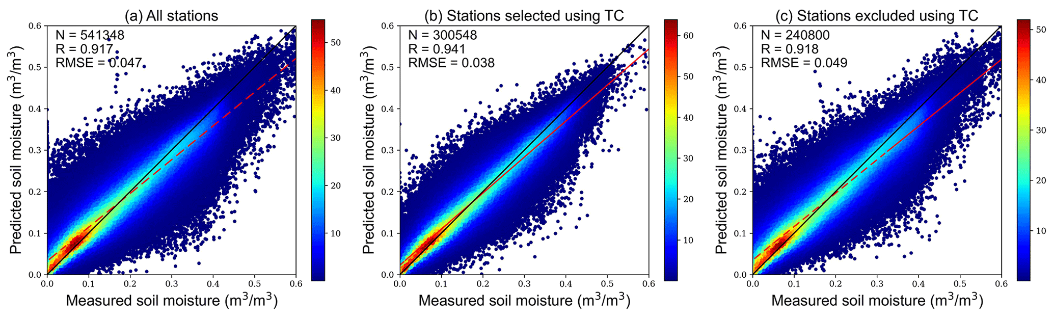
Figure 3Scatterplots of measured and predicted soil moisture from the XGBoost models developed using (a) all ISMN stations, (b) representative stations selected using the TC method, and (c) stations excluded using the TC method. Point colors indicate the probability density. Red dotted line displays the linear regression, and the black solid line is the 1:1 line.
4.2 Model performance on site- or year-independent samples
As can be seen from Table 4, regardless of the type of soil moisture station used during training, model performance on the year-independent test samples (2015 to 2018) decreased significantly compared to that on the random test samples. Among them, the R values of the models trained using all stations and TC-excluded stations were 0.8 and 0.734 for the year-independent test samples, respectively, while the corresponding RMSE increased to 0.07 and 0.084 m3 m−3, respectively. In contrast, the XGBoost model trained using representative stations selected by the TC method achieved the highest accuracy on the year-independent test samples, with R and RMSE values of 0.873 and 0.054 m3 m−3, respectively. Likewise, the performance of the models trained using three different types of stations on the site-independent test samples (randomly selected one-fifth of the total stations) further decreased compared to that of the year-independent test samples. The RMSE values of the models trained using all and excluded stations further increased to 0.093 and 0.106 m3 m−3, respectively, for the site-independent test samples. Alternatively, the XGBoost model trained using representative stations achieved the highest accuracy for the site-independent test samples, with R and RMSE values of 0.715 and 0.079 m3 m−3, respectively. These results suggest that the good performance of the models on the random or year-independent test samples is clearly a result of model overfitting, and their accuracies may degrade significantly when the stations or observation years of the test samples are unknown to them. The relatively lower accuracy achieved by the model on site-independent test samples is least likely to be overfitted and can be regarded as the model's true accuracy. Besides, it appears that increasing the number of stations in the training dataset to account for spatial heterogeneity is more important for improving the models' performance than extending the duration of the measurements to account for temporal dynamics, as also found in a previous study (Zappa et al., 2019). Moreover, training the model with representative stations selected by the TC method can also considerably improve its performance on site- or year-independent test samples, i.e., model performance over unknown time and space.
Table 4Validation accuracy of the XGBoost models trained using three different types of soil moisture stations on three types of test samples.
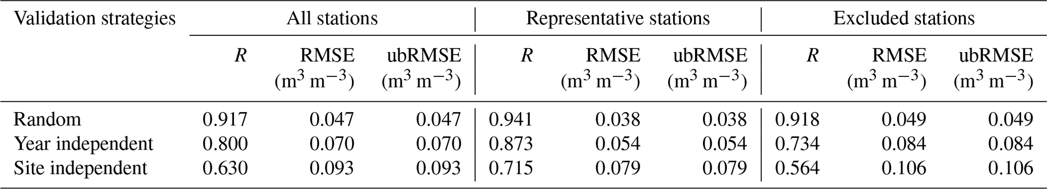
Figure 4 shows the permutation feature importance results of the XGBoost models trained using representative soil moisture stations, which were calculated separately for the three different types of test samples. The permutation importance of an input feature is commonly measured by the degradation of model accuracy when the feature is randomly shuffled (Breiman, 2001), it can be calculated multiple times across a test dataset and is less likely to be biased towards high-cardinality features. Notably, permutation importance does not reflect a feature's intrinsic predictive value but rather its relative importance to a particular model. For all three types of test samples, ERA5-Land surface soil moisture (SM_era) achieved the highest importance score, indicating that this coarse-scale reanalysis soil moisture product can indeed provide reliable soil moisture background information for the 1 km soil moisture estimation model. Specifically, for both the random and year-independent test samples (Fig. 4a, b), the importance of elevation and soil texture variables (sand, silt, and clay) ranked relatively high, showing that soil properties and topographic factors are important for accurate model predictions when the sample locations are known. In addition, the three GLASS black-sky albedo bands (ABD_vis, ABD_nir, and ABD_short) also achieved relatively high importance scores for both types of samples, likely because surface albedo can reflect the surface energy flux and land cover conditions, which are further correlated to the spatial variation in soil moisture (Long et al., 2019). Meanwhile, the importance scores of GLASS LAI and LST were relatively low for the two sample types, which may be partly attributed to their correlation with some high-ranking variables (e.g., ABD_vis, SM_era). For example, after removing ERA5-Land soil moisture from the models, the importance scores of both GLASS LST and LAI increased significantly. In contrast, for the site-independent test samples (Fig. 4c), the importance of ERA5-Land surface soil moisture (SM_era) further increased relative to other variables. In addition, the importance ranking of GLASS albedo and LST increased remarkably, whereas that of terrain and soil texture-related variables dropped dramatically, suggesting that when the location of the test samples is unknown to the model, variables such as coarse-scale soil moisture, albedo, and LST appear to be more important for accurately predicting soil moisture. Note that the final model was developed using all the representative ISMN stations, and its feature importance results over unknown regions could refer to those calculated on the site-independent test samples.
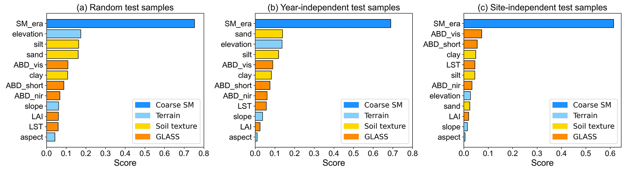
Figure 4Permutation feature importance results of the XGBoost models trained using the representative stations, and calculated using the (a) random, (b) year-independent, and (c) site-independent test samples. Features from different input datasets are divided into four groups with different colors.
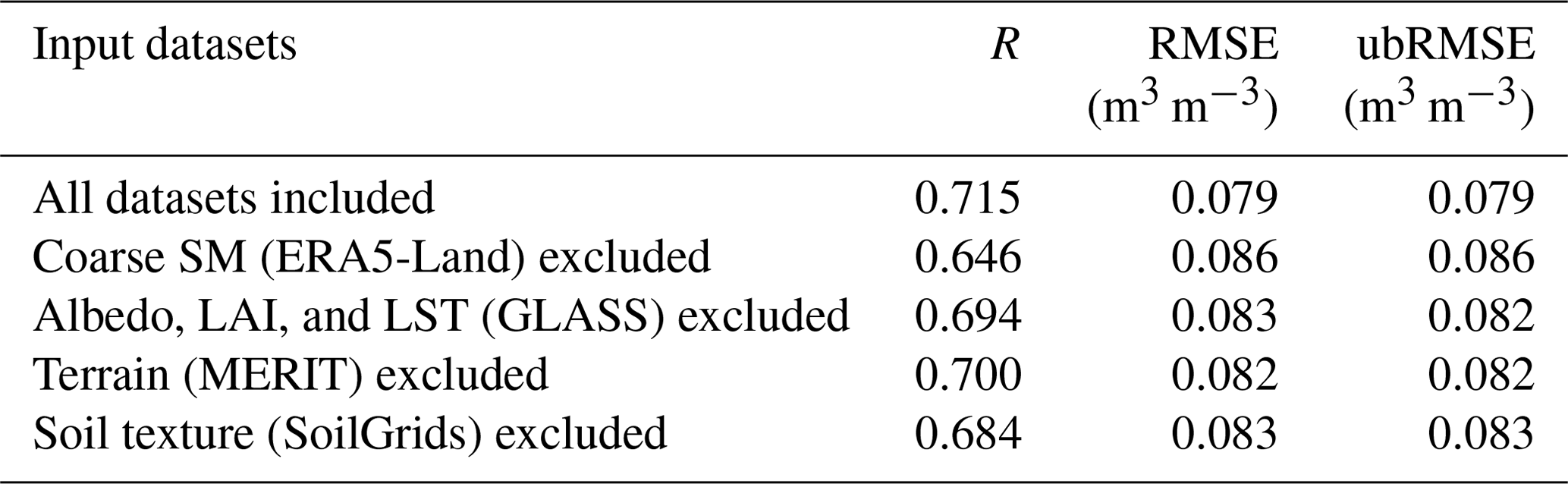
To further investigate the importance of different types of input variables for the 1 km soil moisture estimation model over unknown space, the validation accuracy of the XGBoost models developed using different combinations of input datasets on the site-independent test samples was also compared. The XGBoost model trained with all input datasets achieved the highest accuracy (Table 5), with R and RMSE values of 0.715 and 0.079 m3 m−3, respectively. After the ERA5-Land soil moisture product was excluded, the model accuracy for the test dataset decreased significantly, with the RMSE value increasing to 0.086 m3 m−3, further reflecting the relatively high importance of the coarse-scale soil moisture background information for the 1 km estimation model derived here. Similarly, after excluding GLASS albedo, LAI, and LST from the input variables, the model trained with the remaining variables showed a marked decrease in accuracy for the test dataset, with R and RMSE values of 0.694 and 0.083 m3 m−3, respectively. This indicates that the information on soil and vegetation reflective properties, surface temperature, and vegetation types and densities provided by GLASS products are also important for the 1 km soil moisture estimation model. Further, the exclusion of terrain or soil texture datasets showed a similar effect on model accuracy, with RMSE values decreasing to 0.082 and 0.083 m3 m−3, respectively, again suggesting the pertinent contribution of these variables to improving the performance of the soil moisture estimation model. Besides, as shown in Table 2, the spatial resolution of most input datasets was within 1 km, except for the ERA5-Land product which had a relatively low spatial resolution (0.1∘). Therefore, the integration of multisource input datasets using a machine learning model can improve not only the model accuracy but also the spatial details of the soil moisture product. Because the XGBoost model trained with all input datasets performed best on the test dataset, all datasets were included in model training during the subsequent experiments.
Table 5Performance metrics of the XGBoost model developed using different combinations of input datasets on the site-independent test samples.
To explore the causes of decreased 1 km soil moisture estimation model accuracies over unknown time and space, performance metrics of the models were calculated for each station, which were trained using all ISMN or representative soil moisture stations selected by the TC method. To obtain the validation accuracy for each station, a 5-fold cross-validation method was adopted, where the stations were randomly divided into five folds, with samples from four folds used to develop the model, and the accuracy metrics were derived for the remaining fold. This process was repeated five times, until the accuracies of all stations were evaluated. The distribution of performance metrics for the XGBoost model developed using all stations was dispersed across stations, with R values ranging from −1 to 1, and RMSE values ranging from 0.005 to 0.397 m3 m−3 (Fig. 5, Table 6). Although the median of the bias between model predicted and measured soil moisture was 0, the model exhibited a large prediction bias for most stations (from −0.39 to 0.34 m3 m−3), partly contributing to the large RMSE observed at these stations. After removing the prediction bias for each station, the median ubRMSE of the model decreased to 0.055 m3 m−3, compared to the median RMSE of 0.075 m3 m−3. As a comparison, the performance metrics of the ERA5-Land soil moisture product at each ISMN station were also calculated and are displayed in Fig. 5. The coarse-scale soil moisture product showed similar R values to those of the XGBoost model developed using all stations, and it also yielded large bias and dispersed RMSE and ubRMSE values at most stations.
After filtering the stations using the TC method, the accuracies of the ERA5-Land soil moisture product at those representative stations improved significantly. Similarly, the validation accuracies of the model developed using the representative stations also improved significantly, with the distribution of its performance metrics being more concentrated across stations, compared to the model developed without station filtering. In particular, the median R of the model at each station increased from 0.64 to 0.74, median RMSE decreased from 0.075 to 0.068 m3 m−3, and ubRMSE decreased from 0.055 to 0.052 m3 m−3. Over most of the representative stations, the XGBoost model obtained similar or even larger R values compared to the ERA5-Land soil moisture product. However, there were also several stations where the model achieved relatively lower R values, yet this degradation in temporal metrics with respect to the original coarse-scale products can be found in many soil moisture downscaling studies (Gruber et al., 2020).
On the other hand, the model developed using the representative stations still exhibited a large bias at most stations, ranging from −0.21 to 0.21 m3 m−3, although the median bias of the model was 0. Therefore, the decreased overall accuracies of the model over unknown spaces can be attributed to these large site-specific biases, which may be caused by the high spatiotemporal variability of surface soil moisture and the scale differences between the target point-scale soil moisture and 1 km model predicted soil moisture. Specifically, in random and year-independent validation strategies, part of the site-specific information is known to the models; whereas in the site-independent validation method, this information is entirely unknown to the model. By adopting the TC method, it is possible to select soil moisture stations that are representative of the average soil moisture on a larger scale, thereby alleviating the scale difference issue to some extent. However, there may still be large biases between measurements from these point-scale representative soil moisture stations and footprint-scale average soil moisture values. As these biases are site-specific, can be positive or negative, and have a median value for all samples near 0, the overall ubRMSE that the model achieved on the site- or year-independent test samples can still be large when these biases are unknown to the model. Nevertheless, training the model with representative soil moisture stations not only improved the model's overall performance over unknown spatiotemporal locations (Table 4) but also improved the performance metrics of the model at each station (Fig. 5).
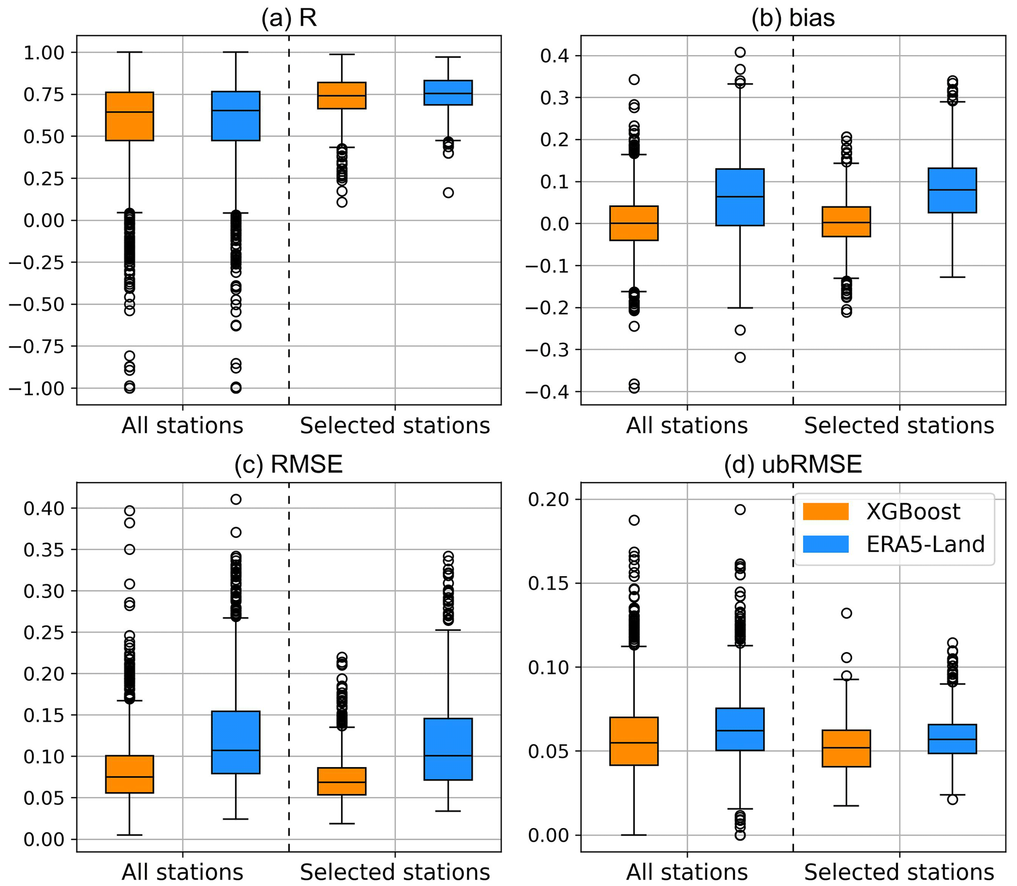
Figure 5Boxplots of the (a) R, (b) bias, (c) RMSE, and (d) ubRMSE achieved by the XGBoost models (blue) developed using all stations and the representative stations selected by the TC method, respectively, in comparison with those of the ERA5-Land soil moisture product (orange).
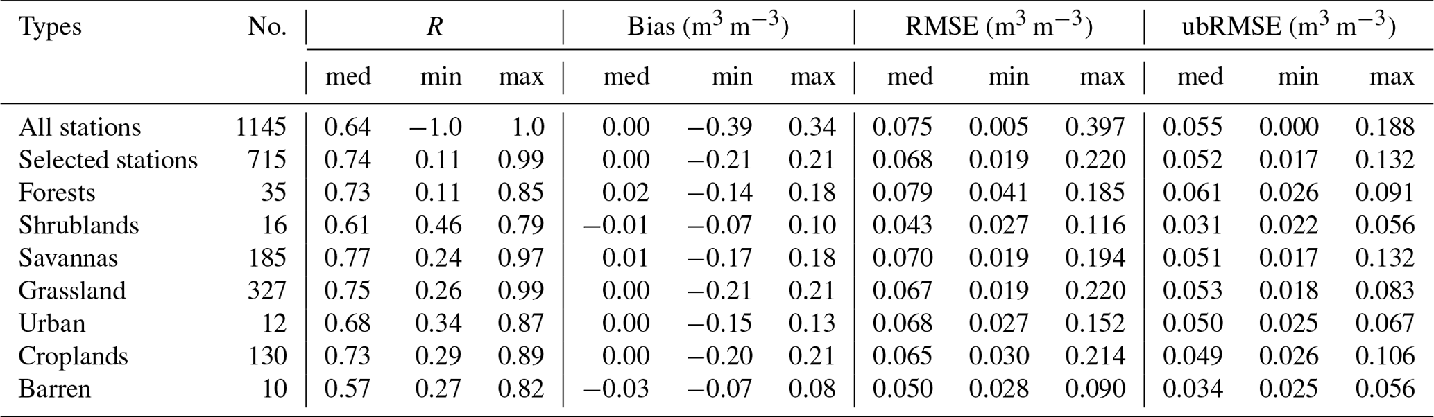
In addition to the performance metrics of the two XGBoost models at each station, Table 6 shows the validation accuracies of the model developed using the representative stations over different land cover types. Affected by a series of practical factors, the distribution of ISMN soil moisture stations is uneven in space, with the majority of the stations located in the CONUS. After screening stations via the TC method, the spatial distribution of representative stations remained uneven, with the resulting number of stations for each land cover type also varying significantly (Fig. 1). Overall, the performance of the model developed using the representative stations for most land cover types showed an improvement compared with the model developed using all stations, as indicated by larger median R values and smaller median RMSE and ubRMSE values. However, the median ubRMSE of the model achieved for forests was larger than that for other land cover types, likely a result of soil moisture maintaining at high levels in forested areas. Additionally, among the seven land cover types, the model achieved the lowest median R values for shrublands and barren lands, likely due to the limited number of stations present across these two types. However, the model also achieved the lowest median ubRMSE values for these two types, which can be partly attributed to the fact that despite the low sample percentages the number of samples for these land cover types was sufficient for the models to learn, as well as in part due to the relatively simple soil moisture dynamics of these two types. Although the median bias of the model for each land cover type was near 0, the model exhibited a large prediction bias for most stations across each land cover type (Table 6). After removing the prediction bias at each station, the median ubRMSE of the model for the seven land cover types ranged from 0.031 to 0.061 m3 m−3, marking a dramatic decrease over the corresponding median RMSE. Given that a large prediction bias existed in each land cover type and that the model performance did not vary significantly across different types, it was suggested that the uneven distribution of land cover types across samples was not the major cause of the decreased overall model accuracy over unknown spaces.
Table 6Performance metric statistics for the XGBoost models developed using all stations and representative stations, as well as those achieved by the latter model over each land cover type.
4.3 Validation of the GLASS SM product on independent networks
Using the XGBoost model developed above, a global 1 km spatiotemporally continuous soil moisture product (GLASS SM) was generated. To intuitively demonstrate the ability of this product for capturing the temporal variations in soil moisture over an unknown space, four independent networks under different climatic and environmental conditions were selected, and the time-series curves of the GLASS and measured soil moisture for these networks were compared. Considering the high spatiotemporal variability of surface soil moisture and the scale differences between point-scale observations and the 1 km GLASS SM product, the mean measured soil moisture curve was first calculated by averaging soil moisture curves from all stations within a network and then compared with the mean predicted soil moisture curve calculated using all corresponding pixels of the GLASS SM product within that network. Moreover, as an input variable of the 1 km soil moisture estimation model, the time-series curves of the ERA5-Land reanalysis soil moisture product over the four independent networks were also extracted as a reference.
In most cases, the GLASS soil moisture curves were much closer to the measured values than the time-series curves of the ERA5-Land reanalysis soil moisture product in both the YA and YB soil moisture networks (Fig. 6a, b). The R values between the GLASS and measured soil moisture for these two networks were 0.84 and 0.89, respectively, which were slightly higher than the ERA5-Land soil moisture (0.80 and 0.84); whereas the ubRMSE values were 0.048 and 0.034 m3 m−3, respectively, slightly lower than the ERA5-Land soil moisture product (0.052 and 0.044 m3 m−3). Accordingly, over these two relatively dense soil moisture networks, the 1 km GLASS SM product can basically capture the dynamics of measured soil moisture. However, underestimates occurred at some high-value intervals on the measured soil moisture curves, which may be caused by nearby irrigation at some stations within agricultural regions, where the GLASS SM product may not be able to capture such patterns, given that irrigation is usually not uniformly distributed in space.
For the Fort Cobb and Little Washita soil moisture networks, both the GLASS and ERA5-Land soil moisture estimates basically captured the dynamics of measured soil moisture (Fig. 6c, d). Specifically, the R values between the mean GLASS and measured soil moisture for these two networks were 0.69 and 0.76, respectively, slightly lower than the ERA5-Land soil moisture product (0.74 and 0.77). However, both the GLASS and ERA5-Land reanalysis soil moisture products showed a large positive bias throughout most of the observation period, particularly in the Little Washita network. This is likely because these two soil moisture networks cover a relatively large watershed containing only a few stations. Nevertheless, the ubRMSE values between the mean GLASS and measured soil moisture values for these two networks were 0.037 and 0.033 m3 m−3, respectively, which were significantly lower than those for the ERA5-Land soil moisture (0.047 and 0.046 m3 m−3). Overall, above results suggested that the derived product can accurately capture the temporal variations of in situ soil moisture under different climatic conditions. Further, the GLASS SM product achieved similar R values as the ERA5-Land product across these networks, with the R values ranging from 0.69 to 0.89 and the ubRMSE values ranging from 0.033 to 0.048 m3 m−3.
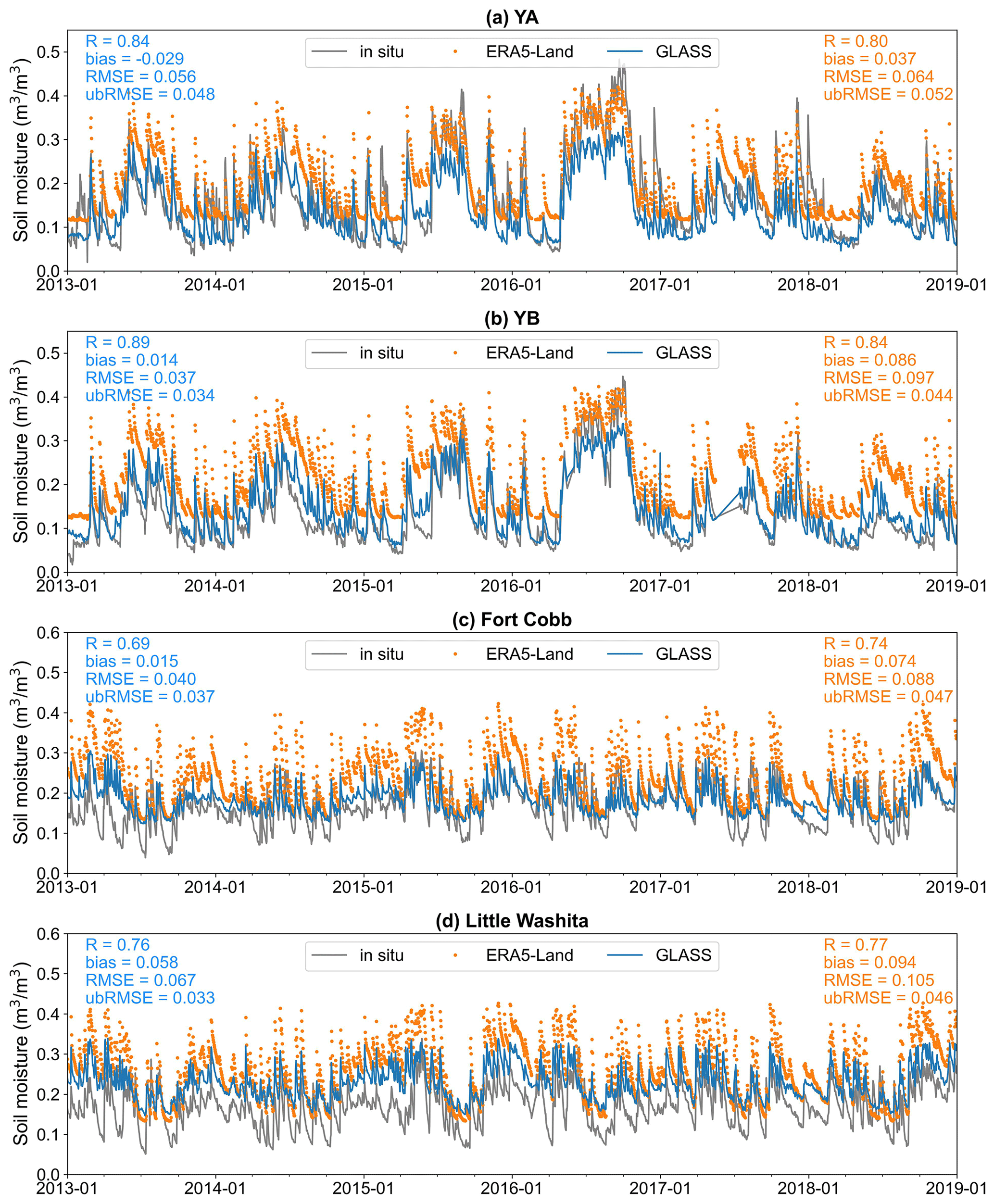
Figure 6Time-series plots of the mean in situ, ERA5-Land, and GLASS soil moisture for four independent soil moisture networks.
4.4 Comparison with existing global soil moisture products
After producing the global 1 km spatiotemporally continuous GLASS SM product, it was compared with two global microwave soil moisture products for spatiotemporal consistency. The first product selected for comparison was SPL2SMAP_S, the first publicly released global soil moisture product at a spatial resolution of 1 km. Because the SPL2SMAP_S 1 km product has a temporal resolution of 12 d over most global areas and as it has many spatial gaps at the daily scale, spatial synthesis of the SPL2SMAP_S dataset was conducted during a 12 d period with relatively high spatial coverage before comparison. Figure 7 shows the spatial distribution of the SPL2SMAP_S 1 km soil moisture product, synthesized from 3 to 15 October 2016, alongside the 1 km spatiotemporally continuous GLASS SM map for 9 October 2016. Here, it can be seen that the 12 d synthetic SPL2SMAP_S soil moisture product still has large spatial gaps (e.g., the western continental United States, western China, and southwestern Australia), whereas the GLASS SM product has a substantially more complete spatial coverage (except for the high-latitude regions during the cold seasons). With regards to the spatial distribution characteristics, both soil moisture products with 1 km resolutions exhibits a high level of consistency, with higher soil moisture levels found in the tropics, eastern USA, and southeastern China and with lower levels observed in deserts (e.g., Sahara) and other semiarid regions.
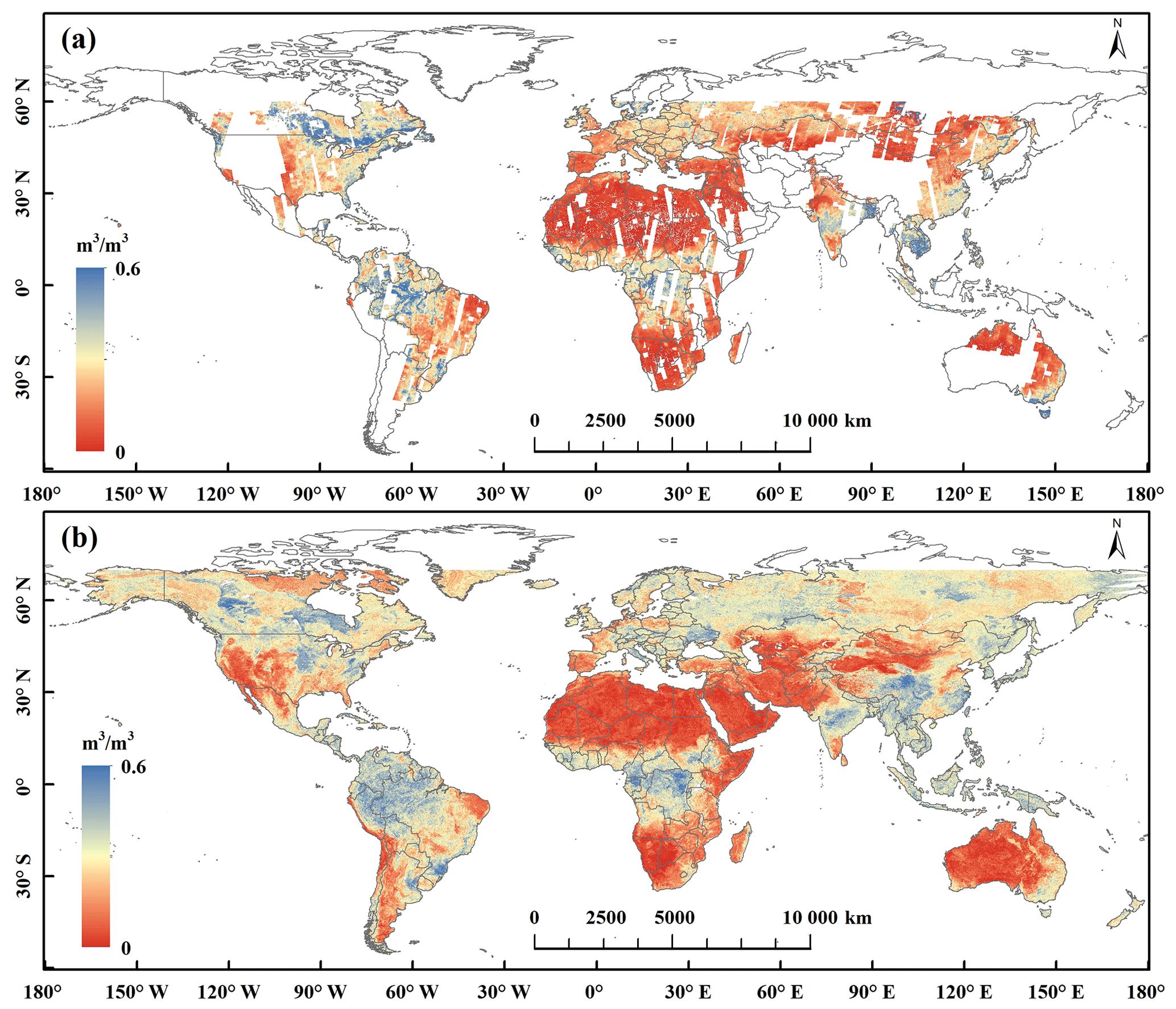
Figure 7(a) The 12 d synthetic SPL2SMAP_S 1 km soil moisture map from 3 to 15 October 2016, and (b) the 1 km spatiotemporally continuous GLASS SM map on 9 October 2016.
To quantitatively investigate the spatial consistency between these two 1 km soil moisture products, spatial R and RMSD between them were calculated for each 12 d of 2016 using collocated pixels, after removing soil moisture estimates larger than 0.6 m3 m−3 from the SPL2SMAP_S product. As displayed in Fig. 8a, the spatial R (orange line) between the GLASS and SPL2SMAP_S products ranges from 0.61 to 0.67, with a median value of 0.62, partially affected by the discontinuous spatial coverage of the SPL2SMAP_S product. The spatial RMSD (orange dots) between the two 1 km products in 2016 ranges from 0.098 to 0.106 m3 m−3, and the relatively large RMSD values may be attributed to the greater spatial heterogeneity (e.g., terrain and soil texture) at fine scales which could cause large disparities in soil moisture estimates from different algorithms. Overall, both qualitative and quantitative comparisons suggested a good and stable spatial consistency between the 1 km GLASS and SPL2SMAP_S microwave soil moisture products.
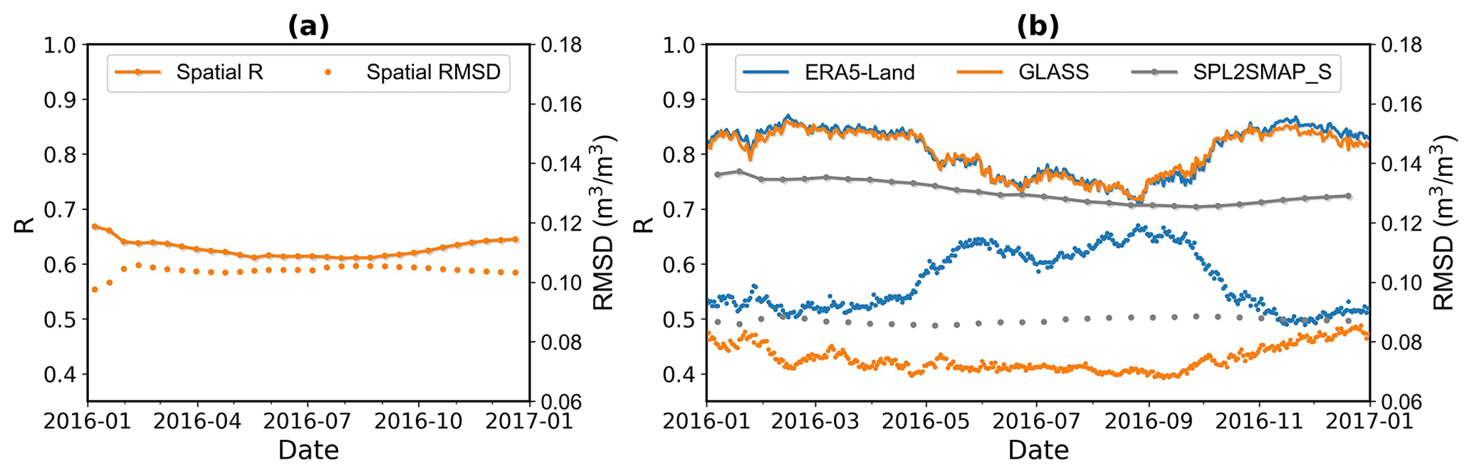
Figure 8Time-series plots of the spatial R (lines) and RMSD (dots) calculated between (a) the GLASS and SPL2SMAP_S soil moisture products at 1 km resolution and (b) the ESA CCI and three resampled soil moisture products (ERA5-Land, GLASS, and SPL2SMAP_S) at 0.25∘ resolution in 2016.
The second global product selected for comparison was the widely used ESA CCI combined soil moisture dataset with a spatial resolution of 0.25∘. Because the CCI soil moisture product has a daily temporal resolution and more complete spatial coverage, more quantitative analyses can be conducted when comparing with the 1 km spatiotemporally continuous GLASS SM product. Figure 9 shows the spatial distribution of the CCI active–passive microwave combined soil moisture and GLASS SM resampled to 0.25∘ for 4 d from different seasons in 2016, as well as the corresponding scatterplots of these two soil moisture products. The high spatial consistency between the CCI soil moisture product and resampled GLASS SM product on different dates is readily apparent, as both products display lower soil moisture values in arid regions, including the western USA, northern and southern Africa, the Middle East, central and western Asia, and Austria, and higher soil moisture values in tropical and temperate regions, such as central Africa, southern Asia, the eastern USA, and southeastern China. Although CCI estimates incorporate a variety of active and passive microwave soil moisture products, its spatial coverage remains incomplete, partly due to observation gaps of the sensors and the physical limitations of microwave soil moisture retrieval algorithms (Dorigo et al., 2017), such as failing to provide accurate soil moisture predictions on densely vegetated land surfaces (e.g., the Amazon River and Congo basins). In contrast, the GLASS SM product shows greater spatial integrity, except at high latitudes in cold seasons due to low temperatures and frozen soils.
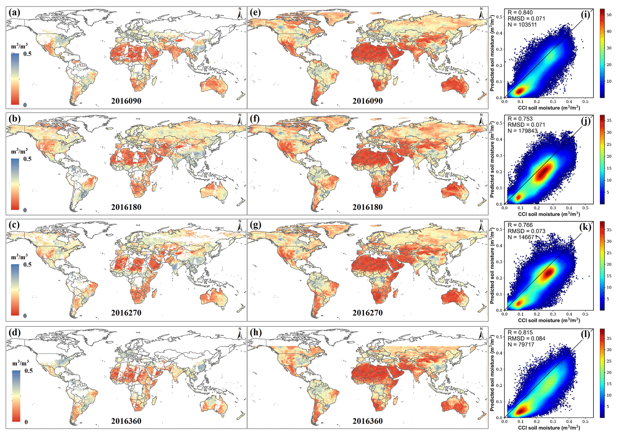
Figure 9(a–d) ESA CCI combined soil moisture maps at 0.25∘, (e–h) the corresponding spatiotemporally continuous GLASS SM maps resampled to 0.25∘, and (i–l) scatterplots of the two products for four Julian dates (90, 180, 270, 360) selected from different seasons of 2016.
As shown in Fig. 8b, the daily spatial R between the resampled GLASS and ESA CCI soil moisture products at 0.25∘ resolution in 2016 ranges from 0.72 to 0.86, with a median value of 0.82, indicating that the two products exhibit high spatial consistency across the seasons. As a comparison, the spatial R and RMSD between the CCI and two other resampled soil moisture products (ERA5-Land and SPL2SMAP_S) were also calculated and plotted. It is clear that the spatial R curves of the resampled ERA5-Land (blue) and GLASS (orange) at 0.25∘ only differ slightly, which is to be expected given that the coarse-scale ERA5-Land soil moisture was used to provide background soil moisture information for our model and given that it achieved the highest importance score among all the input variables. Both curves exhibit significant seasonal variation, with higher spatial R values in spring and winter than in summer or autumn, possibly related to the larger differences between the two resampled products (GLASS and ERA5-Land) and CCI over high latitudes. However, the spatial RMSD curves of the ERA5-Land and GLASS differ significantly. While the blue dotted line (RMSD between CCI and ERA5-Land) exhibits an opposite seasonal pattern to the R curves, with RMSD ranging widely from 0.086 to 0.12 m3 m−3, the orange dotted line (RMSD between CCI and GLASS) is more stable, with RMSD ranging from 0.068 to 0.087 m3 m−3. Besides, as also shown in Fig. 8b, although the resampled SPL2SMAP_S soil moisture product has the most stable spatial R and RMSD curves (gray), it achieves relatively lower spatial R values and larger spatial RMSD values than those of the resampled GLASS product at 0.25∘, suggesting its relatively lower level of spatial consistency with the CCI product. This is to our surprise considering that both the SPL2SMAP_S and CCI soil moisture products were derived from microwave satellite observations, and a possible cause for this could be the discontinuous spatial coverage of the SPL2SMAP_S product.
Note that the GLASS SM product displays a general underestimation relative to the CCI combined soil moisture (Fig. 9i–l). Although the overestimation of the CCI soil moisture product has been reported in a previous study, particularly for equatorial (savanna) regions (Al-Yaari et al., 2019), the GLASS SM product may also contain some biases, which jointly contribute to the RMSD between them. Figure 10 shows a zoomed-in comparison between the 1 km GLASS and 0.25∘ ESA CCI microwave soil moisture product in western China on 28 June 2016, with the corresponding 0.1∘ ERA5-Land reanalysis soil moisture product, which is one of the main inputs to the XGBoost model, also shown as a reference. In general, the GLASS product exhibits spatial consistency with both coarse-scale soil moisture products, with lower soil moisture levels in the Junggar Basin, Tarim Basin, Qaidam Basin, and western part of the Tibetan Plateau, and higher soil moisture levels in the Tianshan Mountains, Ili River valley, and southeastern part of the plateau where the vegetation is also much denser. Specifically, in the southeastern Tibetan Plateau, the GLASS and CCI soil moisture products show higher consistency, while the ERA5-Land soil moisture product is suspected to be underestimated. Moreover, it is clear that the 1 km GLASS SM product is not only spatially complete but also contains more spatial details which can well reflect the distribution patterns of terrain and vegetation.
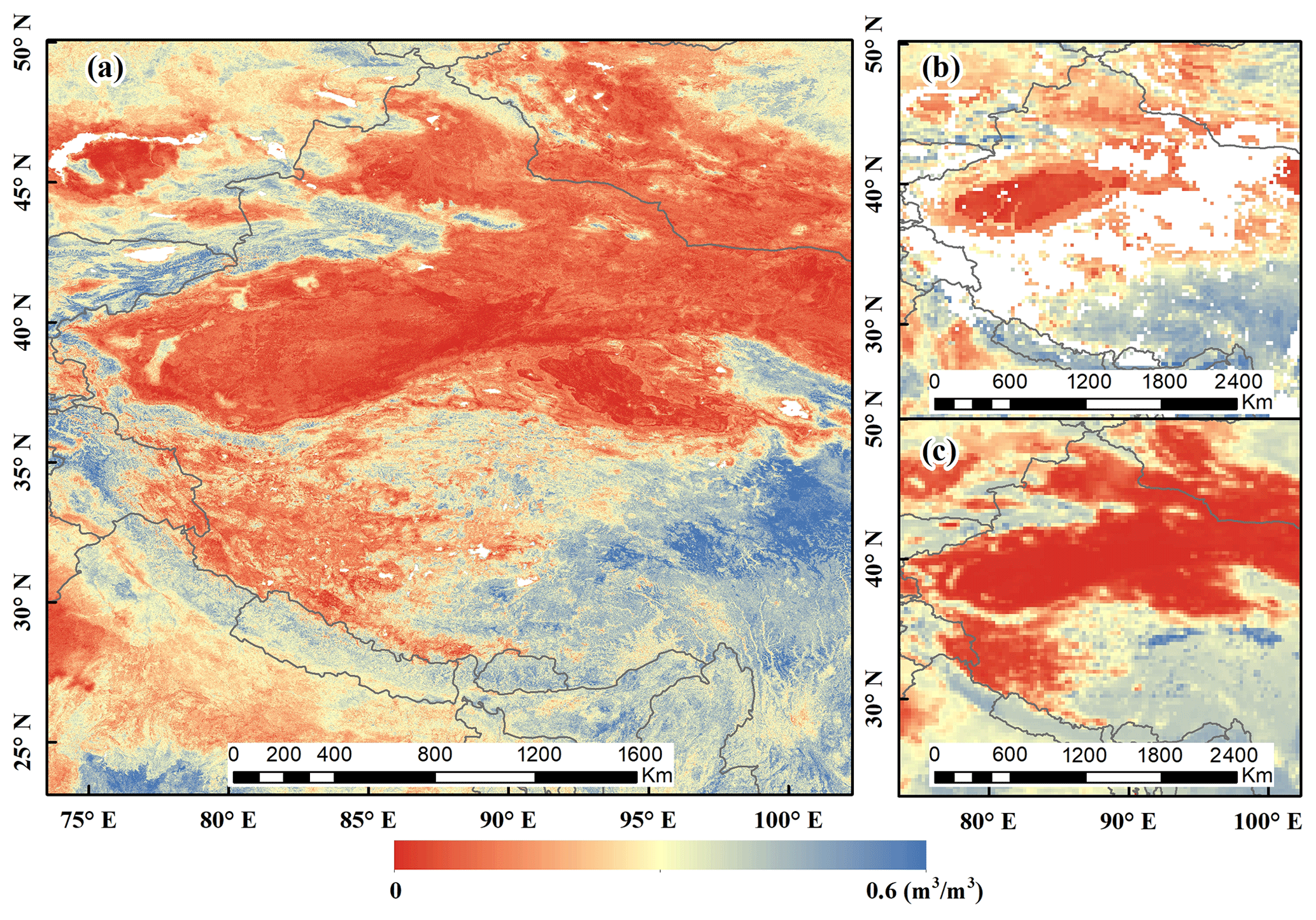
Figure 10Zoomed-in comparison of the (a) 1 km GLASS, (b) 0.25∘ ESA CCI, and (c) 0.1∘ ERA5-Land soil moisture products in western China on 28 June 2016 (the 180th day).
In addition to the spatial consistency analysis described above, the temporal consistency between the CCI and the spatiotemporally continuous GLASS SM product was also explored. Specifically, for each pixel of these two products with > 30 d of concurrent predictions, the R and RMSD between the time-series soil moisture predictions were calculated separately for 2016, and the spatial distribution of these two metrics is shown in Fig. 11. The correlation between the two products was high in most areas, except the Sahara, high latitudes, and some localized regions. The relatively low or even negative R values between the two products in the Sahara is likely due to the fact that soil moisture in this region is close to zero, and a small difference in temporal variation may lead to poor correlation. It can also be seen from Fig. 11b that the RMSD values between the two products in the Sahara were rather small. The relatively low R values between the two products at high latitudes may be attributed to the irregular prediction frequency of the CCI product at high latitudes and the rapid change in soil moisture during the freeze–thaw transition period in this region, which possibly cause larger errors in both products and thus increased temporal inconsistency. Greater differences between soil moisture products at high latitudes have also been found elsewhere (Wang et al., 2021). Further, no obvious patterns were revealed regarding the distribution of RMSD between the two soil moisture products, as the regions with relatively large RMSD values were rather scattered.
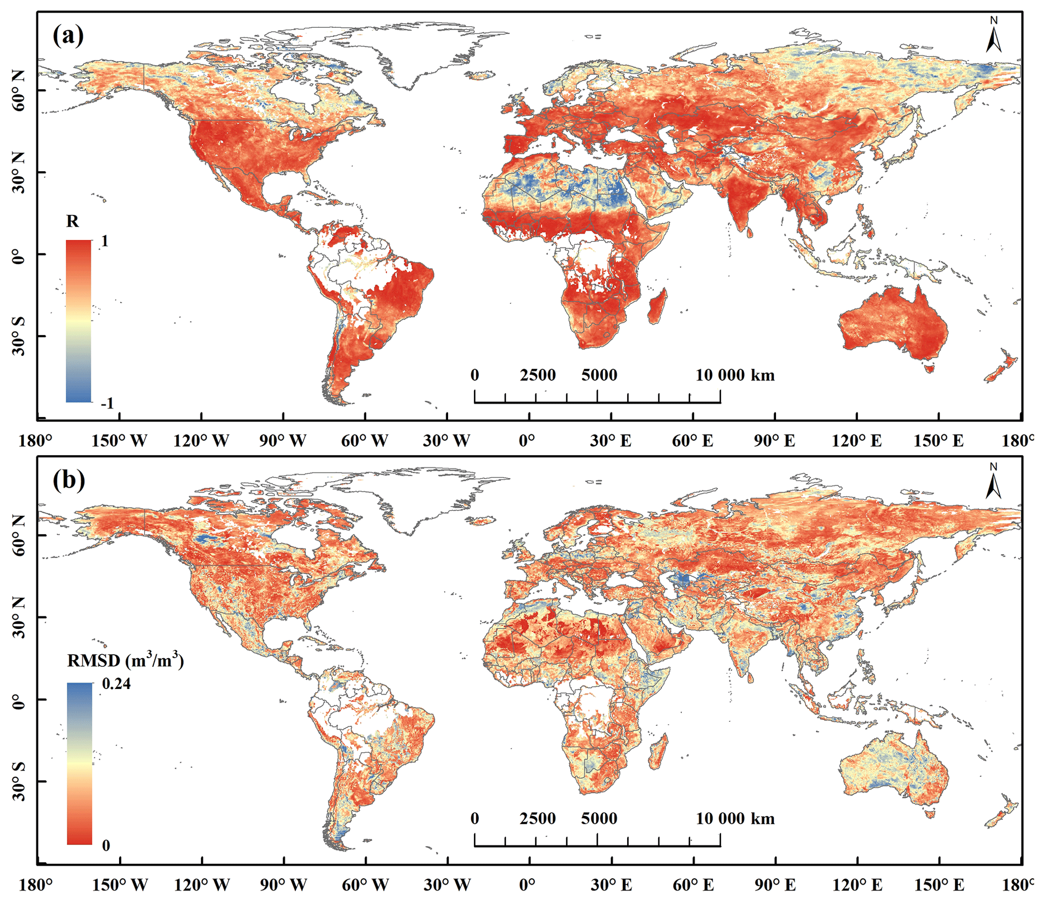
Figure 11The spatial distribution of (a) R and (b) RMSD between the ESA CCI combined soil moisture product and the spatiotemporally continuous GLASS SM product in 2016.
To address the lack of high-resolution, spatiotemporally continuous global soil moisture products, this study developed a global 1 km soil moisture estimation framework which integrated multisource datasets using an XGBoost model. This framework was adapted from the 30 m soil moisture estimation framework proposed by Zhang et al. (2022b), in which the Landsat 8 surface reflectance and thermal observations were replaced with the spatiotemporally continuous GLASS albedo, LST, and LAI products to mitigate the influence of clouds on the spatial continuity and temporal resolution of soil moisture product. Meanwhile, the relatively high temporal resolution of GLASS products allows for much more collocated training samples, which are supposed to alleviate the underestimation of the original 30 m model at high soil moisture levels. In addition, considering the relatively large-scale differences between point-scale in situ soil moisture datasets and GLASS products compared to Landsat datasets, the TC method was adopted to select the representative soil moisture stations, and their measurements were used as the training target of the model. Results showed that the 1 km soil moisture estimation model achieved satisfactory overall accuracy, and training the model with representative stations selected by the TC method can considerably improve its performance over unknown time and space.
Most previous machine-learning-based studies aimed at soil moisture estimation have divided the samples from all observation locations and times randomly into training and test datasets. In this case, the model's accuracy on the random test samples may seem rather high as a result of model overfitting, because these test samples may not be spatially or temporally independent of those in the training dataset, and part of the site-specific information is disclosed to the model. Therefore, model performance must also be fully evaluated using samples from unknown time or space. Senyurek et al. (2020) trained a random forest model using the Cyclone Global Navigation Satellite System observations, as well as the ISMN in situ soil moisture and other geophysical datasets, which was then fully evaluated using 5-fold cross-validation, site-independent, and year-based techniques. Before the model training process, several critical screening conditions were applied to select 106 stations from the 234 ISMN soil moisture stations over the CONUS, and the 5-fold cross-validation R and RMSE of the random forest model were 0.89 and 0.052 m3 m−3, respectively; whereas the site-independent cross-validation R and RMSE values were 0.64 and 0.088 m3 m−3, respectively. Similarly, the overall R and RMSE of the 1 km GLASS SM model for the random and site-independent test samples were 0.941 and 0.038 m3 m−3 and 0.715 and 0.079 m3 m−3, respectively. Notably, Senyurek et al. (2020) attributed the relatively lower site-independent validation accuracy to the fact that different soil moisture stations have distinct climatology, which is difficult for the machine learning model to capture without bias. Instead, we argue that the high validation accuracy achieved by the machine learning models on the random test samples is most likely a result of overfitting, while the relatively lower site-independent validation accuracy is much more realistic. The authors further suggested that model performance could be improved by increasing the representativeness of various land surface conditions within training datasets. Although a representative training dataset is essential for data-driven machine learning models, it was found here that a large prediction bias existed across all land cover types, and the resulting model performance did not vary significantly among them. Therefore, it was concluded here that the site-specific biases induced by scale differences rather than the uneven distribution of land cover types among samples are the major cause of the decreased overall accuracy of the model over unknown time and space.
As emphasized in Gruber et al. (2020), despite the fact that downscaled soil moisture products usually provide more spatial details visually they may not reflect real soil moisture variations, and it is thus necessary to estimate the spatial R for the downscaled products, in addition to temporal analyses. Then, Crow et al. (2022) defined the success of a downscaling algorithm as achieving either better temporal accuracy or spatial skill than the original coarse-scale product that is interpolated onto the fine-scale spatial grid. As can be seen from Fig. 5a, the temporal R values achieved by the XGBoost model at representative stations are similar to those of the coarse-scale ERA5-Land soil moisture product, and Fig. 8b shows that the GLASS and ERA5-Land products achieved similar spatial R values when they are both resampled to 0.25∘ resolution. Therefore, to identify whether the 1 km GLASS SM product actually have added value with respect to the 0.1∘ ERA5-Land product, we also calculated the spatial R for the XGBoost model on a daily basis using soil moisture measurements from representative stations and then compared it with that of the ERA5-Land product interpolated onto the 1 km grid. To make the comparison more rigorous, soil moisture estimated using the 5-fold cross-validation method from the model was adopted to calculate the spatial R instead of the final GLASS SM product (yielding even better results). As displayed in Fig. 12, the spatial R values achieved by the XGBoost model at representative stations improve significantly compared to those of the ERA5-Land product, with the median spatial R increasing from 0.60 to 0.66, and in most cases, the difference in spatial R (R_diff) between the XGBoost model and ERA5-Land product is positive, with a median value of 0.06. Accordingly, it is reasonable to believe that the 1 km GLASS SM product does provide more spatial information which reflects fine-scale soil moisture variations rather than just adding ineffective details.
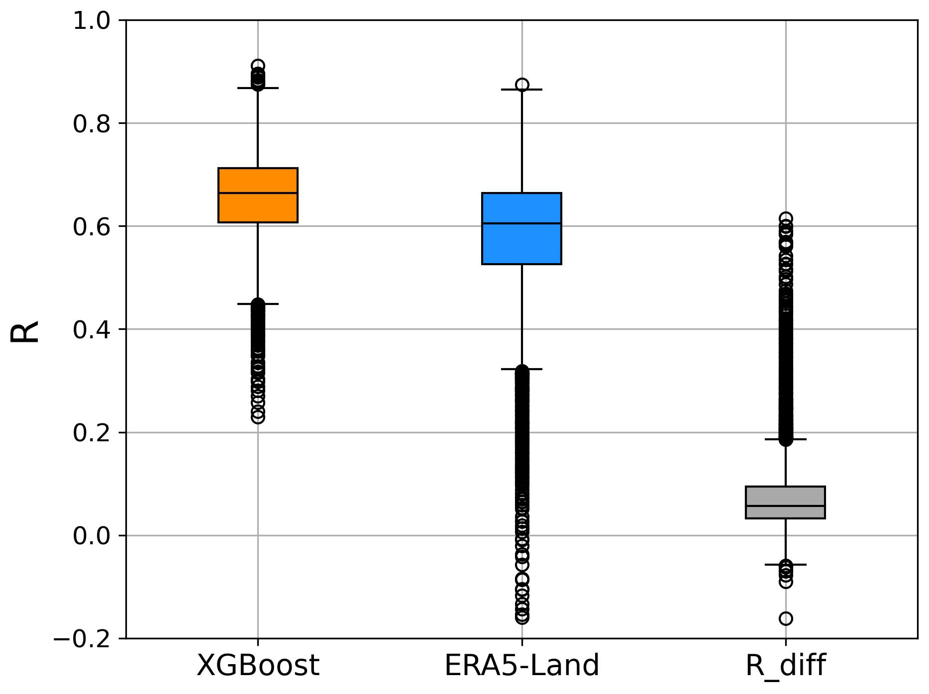
Figure 12Boxplot of the spatial R calculated for the XGBoost model on a daily basis using soil moisture measurements from representative stations, in comparison with those of the ERA5-Land product. The difference in spatial R between the XGBoost model and ERA5-Land product is denoted as R_diff.
To date, several studies have attempted to further improve the accuracy of machine-learning-based soil moisture estimation models through different strategies. Abbaszadeh et al. (2019) classified in situ soil moisture stations within the CONUS according to soil texture class, developing 12 distinct random forest models to downscale the SMAP 36 km soil moisture product using atmospheric, geophysical, and in situ soil moisture datasets. Their downscaled 1 km soil moisture product achieved good overall validation accuracy on both core validation sites and 300 sparse soil moisture stations, with the proposed downscaling approach outperforming the uniform downscaling approach. Similarly, Karthikeyan and Mishra (2021) clustered CONUS into 11 homogeneous regions using a k-means algorithm based on a range of climate and landscape variables, before training an XGBoost model for each region and soil layer to downscale the SMAP Level 4 soil moisture product. Validation at 79 independent soil moisture stations showed that the downscaled product successfully captured temporal variations of measured soil moisture. We also have attempted to classify the ISMN stations based on their soil texture classes or climatic and environmental properties prior to separately developing the models; however, the overall prediction accuracy did not seem to improve significantly.
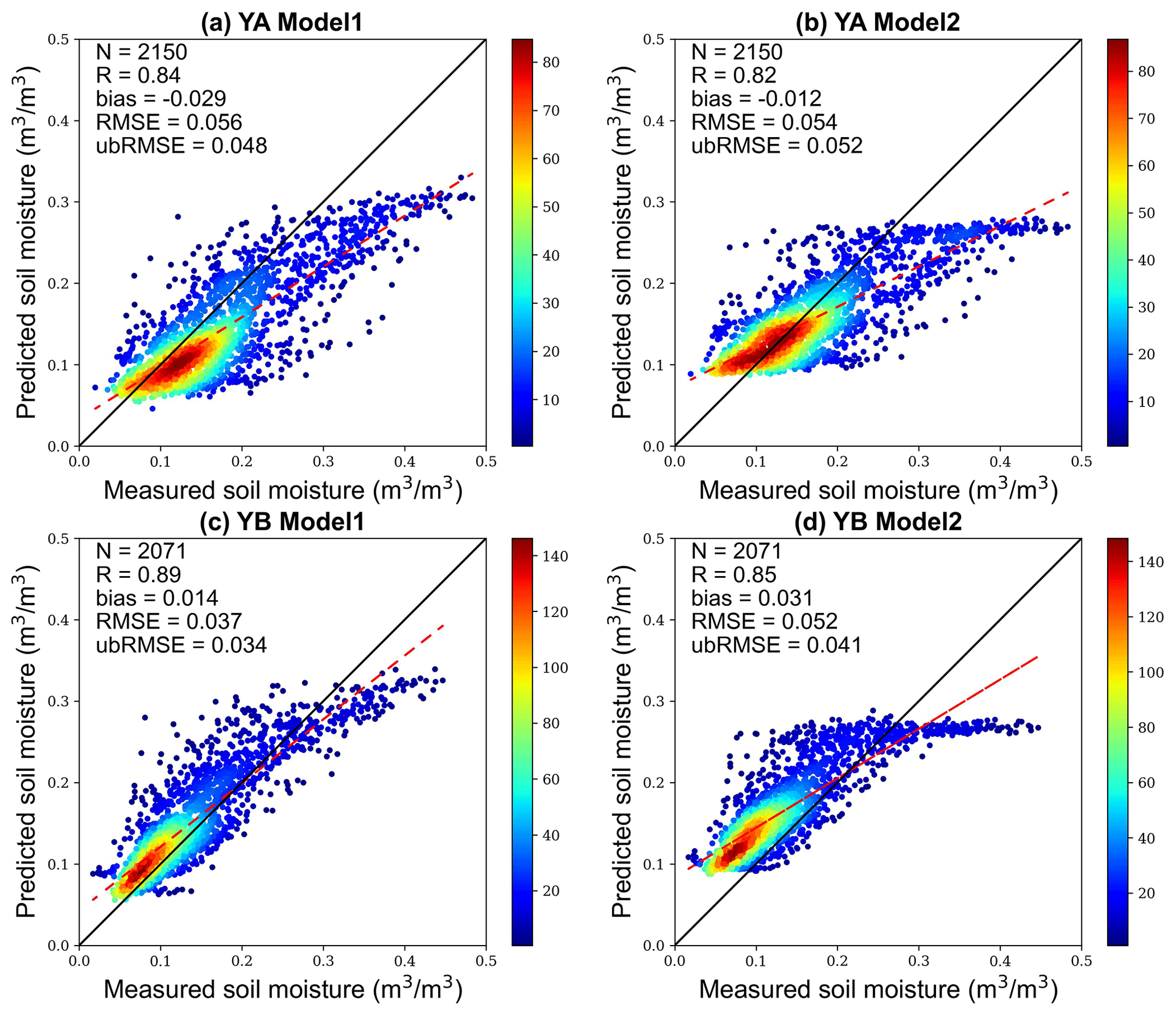
Figure 13Scatterplots of mean measured and predicted soil moisture from different models on the (a–b) YA and (c–d) YB soil moisture networks. Point colors indicate the probability density, whereas the dashed red line is the linear regression, and the solid black line is the 1:1 relationship.
Moreover, to mitigate the impacts of scale differences and improve the prediction accuracy, we also trained a distinct XGBoost model (Model 2) using the average soil moisture of all 30 m pixels within a 1 km pixel where the station was located as the target variable, which was calculated using the 30 m soil moisture estimation model developed by Zhang et al. (2022b). The overall accuracies of Model 2 and the previously developed model trained directly using in situ soil moisture (Model 1) on the YA and YB networks were then compared (Fig. 13). Here, it was found that Model 1 achieved good overall prediction accuracy for both networks. But as also shown in Fig. 6, Model 1 showed slight underestimation at higher soil moisture levels, especially in the YA region. In contrast, while Model 2 obtained similar R values as Model 1 it exhibited much more severe underestimation at higher soil moisture levels in both the YA and YB networks. This may be attributed to the lack of high soil moisture samples in the original 30 m soil moisture estimation model, which were even scarcer after averaging to 1 km. To further improve Model 2 accuracy, uniform global sampling can be performed to generate a large number of 1 km averaged soil moisture samples, but this would be rather labor intensive. Alternatively, the global 1 km GLASS SM product generated using Model 1 accurately captured the temporal variations of the in situ soil moisture, and it exhibited high spatiotemporal consistency with microwave soil moisture products, although some site-specific biases may exist while validating the product against sparse soil moisture stations. Future studies could focus on mitigating the impacts of scale differences on the machine learning models, either by deploying more dense soil moisture monitoring networks, or by further improving the accuracy of high-resolution (e.g., 30 m) but often spatiotemporally discontinuous soil moisture products, and then training the 1 km spatiotemporally continuous GLASS SM model directly using the higher-resolution soil moisture products.
The global daily 1 km spatiotemporally continuous soil moisture product (GLASS SM) from 2000 to 2020 is freely available at http://glass.umd.edu/soil_moisture/ (last access: 12 May 2023). In addition, for user's convenience, the annual average global soil moisture dataset at 1 km resolution was also generated, which can be downloaded from https://doi.org/10.5281/zenodo.7172664 (Zhang et al., 2022a). Note that this product represents the volumetric water content in the uppermost soil layer (0–5 cm). Files are stored in the sinusoidal projection and “GeoTIFF” format.
A global 1 km spatiotemporally continuous soil moisture product (GLASS SM) was derived here using an XGBoost ensemble learning model that integrated multisource datasets, including remotely sensed GLASS products; ERA5-Land reanalysis products, as well as ground-based ISMN soil moisture; and static auxiliary datasets. Validation of the XGBoost model was conducted using three complementary validation strategies, and the GLASS SM product was also evaluated across four independent networks, demonstrating the product's strong capacity to capture temporal dynamics of measured soil moisture. This global 1 km soil moisture product also exhibited high spatiotemporal consistency with two global microwave soil moisture products. Overall, the main findings of the study can be summarized as follows:
-
When the samples from all stations and years were randomly divided into training and test datasets, the XGBoost model achieved a high accuracy on the random test samples. By using the TC method to select representative stations, the validation accuracy of the model was further improved significantly, with an overall R and RMSE of 0.941 and 0.038 m3 m−3, respectively. Nevertheless, such high accuracy achieved by the model on the random test sample is clearly a result of overfitting,
-
Training the model with representative stations selected by the TC method also considerably improved its performance for site- or year-independent samples (i.e., over unknown time and space). The overall validation accuracy of the model trained using representative stations on the site-independent test samples, which was least likely to be overfitted, was an R of 0.715 and RMSE of 0.079 m3 m−3. Compared to the model developed without station filtering, the accuracies of the model trained using representative stations improved significantly on most stations, with the median R and ubRMSE of the model for each station increasing from 0.64 to 0.74 and decreasing from 0.055 to 0.052 m3 m−3, respectively.
-
The time-series validation results of the 1 km GLASS SM product over four independent networks indicated that the product can accurately capture temporal variations in measured soil moisture under different climatic conditions. The GLASS SM product achieved similar R values as the ERA5-Land product, with the R values ranging from 0.69 to 0.89 and the ubRMSE values ranging from 0.033 to 0.048 m3 m−3.
-
Compared with the 1 km SMAP/Sentinel-1 SPL2SMAP_S soil moisture product and the ESA CCI active–passive microwave combined soil moisture product at 0.25∘, the global 1 km spatiotemporally continuous soil moisture product generated here had a more complete spatial coverage, and it exhibited high spatiotemporal consistency with these two products.
The long-term (2000–2020) global GLASS SM product with high spatiotemporal resolution (1 km, daily) and reliable accuracy generated here can benefit climate change studies, hydrological modeling, and agricultural applications at regional and global scales. It is also a valuable complement to currently released global microwave and model-simulated soil moisture datasets. Future studies could consider further improving and fully evaluating the accuracy of the GLASS SM product.
SL and YZ developed the methodology and designed the experiments. YZ, HM, BL, JX, GZ, XL, and CX collected and preprocessed the data. YZ carried out the experiments. YZ, TH, and QW produced the product. YZ prepared the manuscript with contributions from all co-authors.
The contact author has declared that none of the authors has any competing interests.
Publisher's note: Copernicus Publications remains neutral with regard to jurisdictional claims in published maps and institutional affiliations.
We would like to thank the GLASS team for providing albedo, LST, and LAI products; the ECMWF project for offering the ERA5-Land soil moisture product; the SoilGrids project for the soil property dataset; and Yamazaki's team for the MERIT DEM. We also appreciate the scientists and networks who have shared their valuable ground-based soil moisture datasets, as well as the ISMN project for making these datasets readily accessible. We are also very grateful to the editors and reviewers for their valuable suggestions, which helped us a lot to improve the paper.
This study was supported by the Open Research Program of the International Research Center of Big Data for Sustainable Development Goals (grant no. CBAS2022ORP01) and the National Natural Science Foundation of China (grant no. 42090011).
This paper was edited by Kaiguang Zhao and reviewed by three anonymous referees.
Abbaszadeh, P., Moradkhani, H., and Zhan, X.: Downscaling SMAP radiometer soil moisture over the CONUS using an ensemble learning method, Water Resour. Res., 55, 324–344, https://doi.org/10.1029/2018WR023354, 2019.
Al Bitar, A., Mialon, A., Kerr, Y. H., Cabot, F., Richaume, P., Jacquette, E., Quesney, A., Mahmoodi, A., Tarot, S., Parrens, M., Al-Yaari, A., Pellarin, T., Rodriguez-Fernandez, N., and Wigneron, J.-P.: The global SMOS Level 3 daily soil moisture and brightness temperature maps, Earth Syst. Sci. Data, 9, 293–315, https://doi.org/10.5194/essd-9-293-2017, 2017.
Al-Yaari, A., Wigneron, J.-P., Dorigo, W., Colliander, A., Pellarin, T., Hahn, S., Mialon, A., Richaume, P., Fernandez-Moran, R., Fan, L., Kerr, Y. H., and De Lannoy, G.: Assessment and inter-comparison of recently developed/reprocessed microwave satellite soil moisture products using ISMN ground-based measurements, Remote Sens. Environ., 224, 289–303, https://doi.org/10.1016/j.rse.2019.02.008, 2019.
Anderson, W. B., Zaitchik, B. F., Hain, C. R., Anderson, M. C., Yilmaz, M. T., Mecikalski, J., and Schultz, L.: Towards an integrated soil moisture drought monitor for East Africa, Hydrol. Earth Syst. Sci., 16, 2893–2913, https://doi.org/10.5194/hess-16-2893-2012, 2012.
Babaeian, E., Sadeghi, M., Jones, S. B., Montzka, C., Vereecken, H., and Tuller, M.: Ground, Proximal, and Satellite Remote Sensing of Soil Moisture, Rev. Geophys., 57, 530–616, https://doi.org/10.1029/2018RG000618, 2019.
Balenzano, A., Mattia, F., Satalino, G., Lovergine, F. P., Palmisano, D., and Davidson, M. W. J.: Dataset of Sentinel-1 surface soil moisture time series at 1 km resolution over Southern Italy, Data Br., 38, 107345, https://doi.org/10.1016/J.DIB.2021.107345, 2021.
Bartalis, Z., Wagner, W., Naeimi, V., Hasenauer, S., Scipal, K., Bonekamp, H., Figa, J., and Anderson, C.: Initial soil moisture retrievals from the METOP-A Advanced Scatterometer (ASCAT), Geophys. Res. Lett., 34, L20401, https://doi.org/10.1029/2007GL031088, 2007.
Bauer-Marschallinger, B., Freeman, V., Cao, S., Paulik, C., Schaufler, S., Stachl, T., Modanesi, S., Massari, C., Ciabatta, L., Brocca, L., and Wagner, W.: Toward Global Soil Moisture Monitoring With Sentinel-1: Harnessing Assets and Overcoming Obstacles, IEEE T. Geosci. Remote, 57, 520–539, https://doi.org/10.1109/TGRS.2018.2858004, 2019.
Beaudoing, H. and Rodell, M.: GLDAS Noah Land Surface Model L4 3 hourly 0.25 x 0.25 degree V2.1, Goddard Earth Sciences Data and Information Services Center [data set], https://doi.org/10.5067/E7TYRXPJKWOQ, 2020.
Belgiu, M. and Drãguþ, L.: Random forest in remote sensing: A review of applications and future directions, ISPRS J. Photogramm., 114, 24–31, https://doi.org/10.1016/j.isprsjprs.2016.01.011, 2016.
Berg, A. and Sheffield, J.: Climate change and drought: the soil moisture perspective, Current Climate Change Report, 4, 180–191, https://doi.org/10.1007/s40641-018-0095-0, 2018.
Bindlish, R., Jackson, T., Sun, R., Cosh, M., Yueh, S., and Dinardo, S.: Combined Passive and Active Microwave Observations of Soil Moisture During CLASIC, IEEE Geosci. Remote S., 6, 644–648, https://doi.org/10.1109/LGRS.2009.2028441, 2009.
Breiman, L.: Random forests, Mach. Learn., 45, 5–32, https://doi.org/10.1023/A:1010933404324, 2001.
Brocca, L., Ciabatta, L., Massari, C., Camici, S., and Tarpanelli, A.: Soil Moisture for Hydrological Applications: Open Questions and New Opportunities, Water, 9, 140, https://doi.org/10.3390/w9020140, 2017.
Brocca, L., Filippucci, P., Hahn, S., Ciabatta, L., Massari, C., Camici, S., Schüller, L., Bojkov, B., and Wagner, W.: SM2RAIN–ASCAT (2007–2018): global daily satellite rainfall data from ASCAT soil moisture observations, Earth Syst. Sci. Data, 11, 1583–1601, https://doi.org/10.5194/essd-11-1583-2019, 2019.
Chan, S. K., Bindlish, R., O'Neill, P. E., Njoku, E., Jackson, T., Colliander, A., Chen, F., Burgin, M., Dunbar, S., Piepmeier, J., Yueh, S., Entekhabi, D., Cosh, M. H., Caldwell, T., Walker, J., Wu, X., Berg, A., Rowlandson, T., Pacheco, A., McNairn, H., Thibeault, M., Martínez, J., González, Á., Seyfried, M., Bosch, D., Starks, P., Goodrich, D., Prueger, J., Palecki, M., Small, E. E., Zreda, M., Calvet, J., Crow, W. T., and Kerr, Y.: Assessment of the SMAP passive soil moisture product, IEEE T. Geosci. Remote, 54, 4994–5007, https://doi.org/10.1109/TGRS.2016.2561938, 2016.
Chan, S. K., Bindlish, R., O'Neill, P., Jackson, T., Njoku, E., Dunbar, S., Chaubell, J., Piepmeier, J., Yueh, S., Entekhabi, D., Colliander, A., Chen, F., Cosh, M. H., Caldwell, T., Walker, J., Berg, A., McNairn, H., Thibeault, M., Martínez-Fernández, J., Uldall, F., Seyfried, M., Bosch, D., Starks, P., Holifield Collins, C., Prueger, J., van der Velde, R., Asanuma, J., Palecki, M., Small, E. E., Zreda, M., Calvet, J., Crow, W. T., and Kerr, Y.: Development and assessment of the SMAP enhanced passive soil moisture product, Remote Sens. Environ., 204, 931–941, https://doi.org/10.1016/j.rse.2017.08.025, 2018.
Chen, T. and Guestrin, C.: XGBoost: A Scalable Tree Boosting System, in: Proceedings of the 22nd ACM SIGKDD International Conference on Knowledge Discovery and Data Mining, 785–794, https://doi.org/10.1145/2939672.2939785, 2016.
Colliander, A., Jackson, T. J., Bindlish, R., Chan, S., Das, N., Kim, S. B., Cosh, M. H., Dunbar, R. S., Dang, L., Pashaian, L., Asanuma, J., Aida, K., Berg, A., Rowlandson, T., Bosch, D., Caldwell, T., Caylor, K., Goodrich, D., al Jassar, H., Lopez-Baeza, E., Martínez-Fernández, J., González-Zamora, A., Livingston, S., McNairn, H., Pacheco, A., Moghaddam, M., Montzka, C., Notarnicola, C., Niedrist, G., Pellarin, T., Prueger, J., Pulliainen, J., Rautiainen, K., Ramos, J., Seyfried, M., Starks, P., Su, Z., Zeng, Y., van der Velde, R., Thibeault, M., Dorigo, W., Vreugdenhil, M., Walker, J. P., Wu, X., Monerris, A., O'Neill, P. E., Entekhabi, D., Njoku, E. G., and Yueh, S.: Validation of SMAP surface soil moisture products with core validation sites, Remote Sens. Environ., 191, 215–231, https://doi.org/10.1016/j.rse.2017.01.021, 2017.
Crow, W. T., Berg, A. A., Cosh, M. H., Loew, A., Mohanty, B. P., Panciera, R., De Rosnay, P., Ryu, D., and Walker, J. P.: Upscaling sparse ground-based soil moisture observations for the validation of coarse-resolution satellite soil moisture products, Rev. Geophys., 50, 1–20, https://doi.org/10.1029/2011RG000372, 2012.
Crow, W. T., Chen, F., and Colliander, A.: Benchmarking downscaled satellite-based soil moisture products using sparse, point-scale ground observations, Remote Sens. Environ., 283, 113300, https://doi.org/10.1016/j.rse.2022.113300, 2022.
Cui, D., Liang, S., Wang, D., and Liu, Z.: A 1 km global dataset of historical (1979–2013) and future (2020–2100) Köppen–Geiger climate classification and bioclimatic variables, Earth Syst. Sci. Data, 13, 5087–5114, https://doi.org/10.5194/essd-13-5087-2021, 2021.
Dai, Y., Shangguan, W., Wei, N., Xin, Q., Yuan, H., Zhang, S., Liu, S., Lu, X., Wang, D., and Yan, F.: A review of the global soil property maps for Earth system models, SOIL, 5, 137–158, https://doi.org/10.5194/soil-5-137-2019, 2019.
Das, N. N., Entekhabi, D., Dunbar, R. S., Chaubell, M. J., Colliander, A., Yueh, S., Jagdhuber, T., Chen, F., Crow, W., O'Neill, P. E., Walker, J. P., Berg, A., Bosch, D. D., Caldwell, T., Cosh, M. H., Collins, C. H., Lopez-Baeza, E., and Thibeault, M.: The SMAP and Copernicus Sentinel 1A/B microwave active-passive high resolution surface soil moisture product, Remote Sens. Environ., 233, 111380, https://doi.org/10.1016/J.RSE.2019.111380, 2019.
Dorigo, W., Wagner, W., Albergel, C., Albrecht, F., Balsamo, G., Brocca, L., Chung, D., Ertl, M., Forkel, M., Gruber, A., Haas, E., Hamer, P. D., Hirschi, M., Ikonen, J., de Jeu, R., Kidd, R., Lahoz, W., Liu, Y. Y., Miralles, D., Mistelbauer, T., Nicolai-Shaw, N., Parinussa, R., Pratola, C., Reimer, C., van der Schalie, R., Seneviratne, S. I., Smolander, T., and Lecomte, P.: ESA CCI Soil Moisture for improved Earth system understanding: State-of-the art and future directions, Remote Sens. Environ., 203, 185–215, https://doi.org/10.1016/J.RSE.2017.07.001, 2017.
Dorigo, W., Himmelbauer, I., Aberer, D., Schremmer, L., Petrakovic, I., Zappa, L., Preimesberger, W., Xaver, A., Annor, F., Ardö, J., Baldocchi, D., Bitelli, M., Blöschl, G., Bogena, H., Brocca, L., Calvet, J.-C., Camarero, J. J., Capello, G., Choi, M., Cosh, M. C., van de Giesen, N., Hajdu, I., Ikonen, J., Jensen, K. H., Kanniah, K. D., de Kat, I., Kirchengast, G., Kumar Rai, P., Kyrouac, J., Larson, K., Liu, S., Loew, A., Moghaddam, M., Martínez Fernández, J., Mattar Bader, C., Morbidelli, R., Musial, J. P., Osenga, E., Palecki, M. A., Pellarin, T., Petropoulos, G. P., Pfeil, I., Powers, J., Robock, A., Rüdiger, C., Rummel, U., Strobel, M., Su, Z., Sullivan, R., Tagesson, T., Varlagin, A., Vreugdenhil, M., Walker, J., Wen, J., Wenger, F., Wigneron, J. P., Woods, M., Yang, K., Zeng, Y., Zhang, X., Zreda, M., Dietrich, S., Gruber, A., van Oevelen, P., Wagner, W., Scipal, K., Drusch, M., and Sabia, R.: The International Soil Moisture Network: serving Earth system science for over a decade, Hydrol. Earth Syst. Sci., 25, 5749–5804, https://doi.org/10.5194/hess-25-5749-2021, 2021.
Dorigo, W. A., Xaver, A., Vreugdenhil, M., Gruber, A., Hegyiová, A., Sanchis-Dufau, A. D., Zamojski, D., Cordes, C., Wagner, W., and Drusch, M.: Global Automated Quality Control of In Situ Soil Moisture Data from the International Soil Moisture Network, Vadose Zone J., 12, vzj2012.0097, https://doi.org/10.2136/vzj2012.0097, 2013.
Entekhabi, D., Reichle, R. H., Koster, R. D., and Crow, W. T.: Performance metrics for soil moisture retrievals and application requirements, J. Hydrometeorol., 11, 832–840, https://doi.org/10.1175/2010JHM1223.1, 2010.
Friedl, M. and Sulla-Menashe, D.: MCD12Q1 MODIS/Terra+Aqua Land Cover Type Yearly L3 Global 500m SIN Grid V006, NASA EOSDIS Land Processes DAAC [data set], https://doi.org/10.5067/MODIS/MCD12Q1.006, 2019.
Friedman, J. H.: Greedy function approximation: a gradient boosting machine, Ann. Stat., 29, 1189–1232, https://doi.org/10.1214/aos/1013203451, 2001.
Ghulam, A., Qin, Q., Teyip, T., and Li, Z.-L.: Modified perpendicular drought index (MPDI): a real-time drought monitoring method, ISPRS J. Photogramm., 62, 150–164, https://doi.org/10.1016/j.isprsjprs.2007.03.002, 2007.
Gislason, P. O., Benediktsson, J. A., and Sveinsson, J. R.: Random Forests for land cover classification, Pattern Recognit. Lett., 27, 294–300, https://doi.org/10.1016/j.patrec.2005.08.011, 2006.
Gruber, A., Dorigo, W. A., Zwieback, S., Xaver, A., and Wagner, W.: Characterizing Coarse-Scale Representativeness of in situ Soil Moisture Measurements from the International Soil Moisture Network, Vadose Zone J., 12, vzj2012.0170, https://doi.org/10.2136/vzj2012.0170, 2013.
Gruber, A., Su, C.-H., Zwieback, S., Crow, W., Dorigo, W., and Wagner, W.: Recent advances in (soil moisture) triple collocation analysis, Int. J. Appl. Earth Obs., 45, 200–211, https://doi.org/10.1016/j.jag.2015.09.002, 2016.
Gruber, A., Scanlon, T., van der Schalie, R., Wagner, W., and Dorigo, W.: Evolution of the ESA CCI Soil Moisture climate data records and their underlying merging methodology, Earth Syst. Sci. Data, 11, 717–739, https://doi.org/10.5194/essd-11-717-2019, 2019.
Gruber, A., De Lannoy, G., Albergel, C., Al-Yaari, A., Brocca, L., Calvet, J.-C., Colliander, A., Cosh, M., Crow, W., Dorigo, W., Draper, C., Hirschi, M., Kerr, Y., Konings, A., Lahoz, W., McColl, K., Montzka, C., Muñoz-Sabater, J., Peng, J., Reichle, R., Richaume, P., Rüdiger, C., Scanlon, T., van der Schalie, R., Wigneron, J.-P., and Wagner, W.: Validation practices for satellite soil moisture retrievals: What are (the) errors?, Remote Sens. Environ., 244, 111806, https://doi.org/10.1016/j.rse.2020.111806, 2020.
Hersbach, H., Bell, B., Berrisford, P., Hirahara, S., Horányi, A., Muñoz-Sabater, J., Nicolas, J., Peubey, C., Radu, R., Schepers, D., Simmons, A., Soci, C., Abdalla, S., Abellan, X., Balsamo, G., Bechtold, P., Biavati, G., Bidlot, J., Bonavita, M., De Chiara, G., Dahlgren, P., Dee, D., Diamantakis, M., Dragani, R., Flemming, J., Forbes, R., Fuentes, M., Geer, A., Haimberger, L., Healy, S., Hogan, R. J., Hólm, E., Janisková, M., Keeley, S., Laloyaux, P., Lopez, P., Lupu, C., Radnoti, G., de Rosnay, P., Rozum, I., Vamborg, F., Villaume, S., and Thépaut, J.-N.: The ERA5 global reanalysis, Q. J. Roy. Meteor. Soc., 146, 1999–2049, https://doi.org/10.1002/qj.3803, 2020.
Holzman, M. E., Rivas, R., and Piccolo, M. C.: Estimating soil moisture and the relationship with crop yield using surface temperature and vegetation index, Int. J. Appl. Earth Obs., 28, 181–192, https://doi.org/10.1016/j.jag.2013.12.006, 2014.
Humphrey, V., Berg, A., Ciais, P., Gentine, P., Jung, M., Reichstein, M., Seneviratne, S. I., and Frankenberg, C.: Soil moisture–atmosphere feedback dominates land carbon uptake variability, Nature, 592, 65–69, https://doi.org/10.1038/s41586-021-03325-5, 2021.
Karthikeyan, L. and Mishra, A. K.: Multi-layer high-resolution soil moisture estimation using machine learning over the United States, Remote Sens. Environ., 266, 112706, https://doi.org/10.1016/J.RSE.2021.112706, 2021.
Kerr, Y. H., Al-Yaari, A., Rodriguez-Fernandez, N., Parrens, M., Molero, B., Leroux, D., Bircher, S., Mahmoodi, A., Mialon, A., Richaume, P., Delwart, S., Al Bitar, A., Pellarin, T., Bindlish, R., Jackson, T. J., Rüdiger, C., Waldteufel, P., Mecklenburg, S., and Wigneron, J. P.: Overview of SMOS performance in terms of global soil moisture monitoring after six years in operation, Remote Sens. Environ., 180, 40–63, https://doi.org/10.1016/j.rse.2016.02.042, 2016.
Kim, S., Zhang, R., Pham, H., and Sharma, A.: A Review of Satellite-Derived Soil Moisture and Its Usage for Flood Estimation, Remote Sens. Earth Syst. Sci., 2, 225–246, https://doi.org/10.1007/s41976-019-00025-7, 2019.
Li, B., Liang, S., Liu, X., Ma, H., Chen, Y., Liang, T., and He, T.: Estimation of all-sky 1 km land surface temperature over the conterminous United States, Remote Sens. Environ., 266, 112707, https://doi.org/10.1016/J.RSE.2021.112707, 2021.
Li, X., Wigneron, J.-P., Fan, L., Frappart, F., Yueh, S. H., Colliander, A., Ebtehaj, A., Gao, L., Fernandez-Moran, R., Liu, X., Wang, M., Ma, H., Moisy, C., and Ciais, P.: A new SMAP soil moisture and vegetation optical depth product (SMAP-IB): Algorithm, assessment and inter-comparison, Remote Sens. Environ., 271, 112921, https://doi.org/10.1016/j.rse.2022.112921, 2022.
Liang, S. and Wang, J. (Eds.): Chapter 18 – Soil moisture contents, in: Advanced Remote Sensing, 2nd Edn., Academic Press, 685–711, https://doi.org/10.1016/B978-0-12-815826-5.00018-0, 2020.
Liang, S., Cheng, J., Jia, K., Jiang, B., Liu, Q., Xiao, Z., Yao, Y., Yuan, W., Zhang, X., Zhao, X., and Zhou, J.: The Global Land Surface Satellite (GLASS) Product Suite, B. Am. Meteorol. Soc., 102, E323–E337, https://doi.org/10.1175/BAMS-D-18-0341.1, 2021.
Liu, L., Gudmundsson, L., Hauser, M., Qin, D., Li, S., and Seneviratne, S. I.: Soil moisture dominates dryness stress on ecosystem production globally, Nat. Commun., 11, 4892, https://doi.org/10.1038/s41467-020-18631-1, 2020.
Liu, N. F., Liu, Q., Wang, L. Z., Liang, S. L., Wen, J. G., Qu, Y., and Liu, S. H.: A statistics-based temporal filter algorithm to map spatiotemporally continuous shortwave albedo from MODIS data, Hydrol. Earth Syst. Sci., 17, 2121–2129, https://doi.org/10.5194/hess-17-2121-2013, 2013.
Long, D., Bai, L., Yan, L., Zhang, C., Yang, W., Lei, H., Quan, J., Meng, X., and Shi, C.: Generation of spatially complete and daily continuous surface soil moisture of high spatial resolution, Remote Sens. Environ., 233, 111364, https://doi.org/10.1016/j.rse.2019.111364, 2019.
Luo, P., Song, Y., Huang, X., Ma, H., Liu, J., Yao, Y., and Meng, L.: Identifying determinants of spatio-temporal disparities in soil moisture of the Northern Hemisphere using a geographically optimal zones-based heterogeneity model, ISPRS J. Photogramm., 185, 111–128, https://doi.org/10.1016/j.isprsjprs.2022.01.009, 2022.
Ma, H. and Liang, S.: Development of the GLASS 250-m leaf area index product (version 6) from MODIS data using the bidirectional LSTM deep learning model, Remote Sens. Environ., 273, 112985, https://doi.org/10.1016/J.RSE.2022.112985, 2022.
Ma, H., Zeng, J., Zhang, X., Fu, P., Zheng, D., Wigneron, J.-P., Chen, N., and Niyogi, D.: Evaluation of six satellite- and model-based surface soil temperature datasets using global ground-based observations, Remote Sens. Environ., 264, 112605, https://doi.org/10.1016/j.rse.2021.112605, 2021.
McColl, K. A., Vogelzang, J., Konings, A. G., Entekhabi, D., Piles, M., and Stoffelen, A.: Extended triple collocation: Estimating errors and correlation coefficients with respect to an unknown target, Geophys. Res. Lett., 41, 6229–6236, https://doi.org/10.1002/2014GL061322, 2014.
Molero, B., Leroux, D. J., Richaume, P., Kerr, Y. H., Merlin, O., Cosh, M. H., and Bindlish, R.: Multi-Timescale Analysis of the Spatial Representativeness of In Situ Soil Moisture Data within Satellite Footprints, J. Geophys. Res.-Atmos., 123, 3–21, https://doi.org/10.1002/2017JD027478, 2018.
Muñoz-Sabater, J.: ERA5-Land hourly data from 1981 to present, Copernicus Climate Change Service (C3S) Climate Data Store (CDS) [data set], https://doi.org/10.24381/cds.e2161bac, 2019.
Muñoz-Sabater, J.: ERA5-Land hourly data from 1950 to 1980, Copernicus Climate Change Service (C3S) Climate Data Store (CDS) [data set], https://doi.org/10.24381/cds.e2161bac, 2021.
Muñoz-Sabater, J., Dutra, E., Agustí-Panareda, A., Albergel, C., Arduini, G., Balsamo, G., Boussetta, S., Choulga, M., Harrigan, S., Hersbach, H., Martens, B., Miralles, D. G., Piles, M., Rodríguez-Fernández, N. J., Zsoter, E., Buontempo, C., and Thépaut, J.-N.: ERA5-Land: a state-of-the-art global reanalysis dataset for land applications, Earth Syst. Sci. Data, 13, 4349–4383, https://doi.org/10.5194/essd-13-4349-2021, 2021.
Naz, B. S., Kollet, S., Franssen, H.-J. H., Montzka, C., and Kurtz, W.: A 3 km spatially and temporally consistent European daily soil moisture reanalysis from 2000 to 2015, Sci. Data, 7, 111, https://doi.org/10.1038/s41597-020-0450-6, 2020.
Njoku, E. G., Jackson, T. J., Lakshmi, V., Chan, T. K., and Nghiem, S. V: Soil moisture retrieval from AMSR-E, IEEE T. Geosci. Remote, 41, 215–229, https://doi.org/10.1109/TGRS.2002.808243, 2003.
O'Neill, P. E., Chan, S., Njoku, E. G., Jackson, T., Bindlish, R., and Chaubell, J.: SMAP L3 Radiometer Global Daily 36 km EASE-Grid Soil Moisture, Version 8, NASA National Snow and Ice Data Center Distributed Active Archive Center [data set], https://doi.org/10.5067/OMHVSRGFX38O, 2021.
Owe, M., de Jeu, R., and Holmes, T.: Multisensor historical climatology of satellite-derived global land surface moisture, J. Geophys. Res.-Earth, 113, F01002, https://doi.org/10.1029/2007JF000769, 2008.
Peng, J., Loew, A., Merlin, O., and Verhoest, N. E. C.: A review of spatial downscaling of satellite remotely sensed soil moisture, Rev. Geophys., 55, 341–366, https://doi.org/10.1002/2016RG000543, 2017.
Peng, J., Albergel, C., Balenzano, A., Brocca, L., Cartus, O., Cosh, M. H., Crow, W. T., Dabrowska-Zielinska, K., Dadson, S., Davidson, M. W. J., de Rosnay, P., Dorigo, W., Gruber, A., Hagemann, S., Hirschi, M., Kerr, Y. H., Lovergine, F., Mahecha, M. D., Marzahn, P., Mattia, F., Musial, J. P., Preuschmann, S., Reichle, R. H., Satalino, G., Silgram, M., van Bodegom, P. M., Verhoest, N. E. C., Wagner, W., Walker, J. P., Wegmüller, U., and Loew, A.: A roadmap for high-resolution satellite soil moisture applications – confronting product characteristics with user requirements, Remote Sens. Environ., 252, 112162, https://doi.org/10.1016/J.RSE.2020.112162, 2021.
Poggio, L., de Sousa, L. M., Batjes, N. H., Heuvelink, G. B. M., Kempen, B., Ribeiro, E., and Rossiter, D.: SoilGrids 2.0: producing soil information for the globe with quantified spatial uncertainty, SOIL, 7, 217–240, https://doi.org/10.5194/soil-7-217-2021, 2021.
Qu, Y., Liu, Q., Liang, S., Wang, L., Liu, N., and Liu, S.: Direct-Estimation Algorithm for Mapping Daily Land-Surface Broadband Albedo From MODIS Data, IEEE T. Geosci. Remote, 52, 907–919, https://doi.org/10.1109/TGRS.2013.2245670, 2014.
Rahimzadeh-Bajgiran, P., Berg, A. A., Champagne, C., and Omasa, K.: Estimation of soil moisture using optical/thermal infrared remote sensing in the Canadian Prairies, ISPRS J. Photogramm., 83, 94–103, https://doi.org/10.1016/j.isprsjprs.2013.06.004, 2013.
Rodell, M., Houser, P. R., Jambor, U., Gottschalck, J., Mitchell, K., Meng, C. J., Arsenault, K., Cosgrove, B., Radakovich, J., Bosilovich, M., Entin, J. K., Walker, J. P., Lohmann, D., and Toll, D.: The global land data assimilation system, B. Am. Meteorol. Soc., 85, 381–394, https://doi.org/10.1175/BAMS-85-3-381, 2004.
Senyurek, V., Lei, F., Boyd, D., Kurum, M., Gurbuz, A. C., and Moorhead, R.: Machine Learning-Based CYGNSS Soil Moisture Estimates over ISMN sites in CONUS, Remote Sens., 12, 1168, https://doi.org/10.3390/rs12071168, 2020.
Sheffield, J., Goteti, G., Wen, F., and Wood, E. F.: A simulated soil moisture based drought analysis for the United States, J. Geophys. Res., 109, 1–19, https://doi.org/10.1029/2004JD005182, 2004.
Shi, J., Zhao, T., Cui, Q., and Yao, P.: Airborne and Spaceborne Passive Microwave Measurements of Soil Moisture, in: Observation and Measurement of Ecohydrological Processes, edited by: Li, X. and Vereecken, H., Springer Berlin Heidelberg, Berlin, Heidelberg, 71–105, https://doi.org/10.1007/978-3-662-48297-1_3, 2019.
Smith, A. B., Walker, J. P., Western, A. W., Young, R. I., Ellett, K. M., Pipunic, R. C., Grayson, R. B., Siriwardena, L., Chiew, F. H. S., and Richter, H.: The Murrumbidgee soil moisture monitoring network data set, Water Resour. Res., 48, W07701, https://doi.org/10.1029/2012WR011976, 2012.
Song, J.: Bias corrections for Random Forest in regression using residual rotation, J. Korean Stat. Soc., 44, 321–326, https://doi.org/10.1016/j.jkss.2015.01.003, 2015.
Song, P., Zhang, Y., Guo, J., Shi, J., Zhao, T., and Tong, B.: A 1 km daily surface soil moisture dataset of enhanced coverage under all-weather conditions over China in 2003–2019, Earth Syst. Sci. Data, 14, 2613–2637, https://doi.org/10.5194/essd-14-2613-2022, 2022.
Starks, P. J., Fiebrich, C. A., Grimsley, D. L., Garbrecht, J. D., Steiner, J. L., Guzman, J. A., and Moriasi, D. N.: Upper Washita River Experimental Watersheds: Meteorologic and Soil Climate Measurement Networks, J. Environ. Qual., 43, 1239–1249, https://doi.org/10.2134/jeq2013.08.0312, 2014.
Stoffelen, A.: Toward the true near-surface wind speed: Error modeling and calibration using triple collocation, J. Geophys. Res.-Oceans, 103, 7755–7766, https://doi.org/10.1029/97JC03180, 1998.
Vergopolan, N., Chaney, N. W., Pan, M., Sheffield, J., Beck, H. E., Ferguson, C. R., Torres-Rojas, L., Sadri, S., and Wood, E. F.: SMAP-HydroBlocks, a 30-m satellite-based soil moisture dataset for the conterminous US, Sci. Data, 8, 264, https://doi.org/10.1038/s41597-021-01050-2, 2021.
Wagner, W., Pathe, C., Doubkova, M., Sabel, D., Bartsch, A., Hasenauer, S., Blöschl, G., Scipal, K., Martínez-Fernández, J., and Löw, A.: Temporal Stability of Soil Moisture and Radar Backscatter Observed by the Advanced Synthetic Aperture Radar (ASAR), Sensors, 8, 1174–1197, https://doi.org/10.3390/s80201174, 2008.
Wagner, W., Hahn, S., Kidd, R., Melzer, T., Bartalis, Z., Hasenauer, S., Figa-Saldaña, J., de Rosnay, P., Jann, A., Schneider, S., Komma, J., Kubu, G., Brugger, K., Aubrecht, C., Züger, J., Gangkofner, U., Kienberger, S., Brocca, L., Wang, Y., Blöschl, G., Eitzinger, J., and Steinnocher, K.: The ASCAT Soil Moisture Product: A Review of its Specifications, Validation Results, and Emerging Applications, Meteorol. Z., 22, 5–33, https://doi.org/10.1127/0941-2948/2013/0399, 2013.
Wang, Y., Leng, P., Peng, J., Marzahn, P., and Ludwig, R.: Global assessments of two blended microwave soil moisture products CCI and SMOPS with in-situ measurements and reanalysis data, Int. J. Appl. Earth Obs., 94, 102234, https://doi.org/10.1016/J.JAG.2020.102234, 2021.
Wigneron, J.-P., Li, X., Frappart, F., Fan, L., Al-Yaari, A., De Lannoy, G., Liu, X., Wang, M., Le Masson, E., and Moisy, C.: SMOS-IC data record of soil moisture and L-VOD: Historical development, applications and perspectives, Remote Sens. Environ., 254, 112238, https://doi.org/10.1016/j.rse.2020.112238, 2021.
Xu, X.: Evaluation of SMAP Level 2, 3, and 4 Soil Moisture Datasets over the Great Lakes Region, Remote Sensing, 12, 3785, https://doi.org/10.3390/rs12223785, 2020.
Yamazaki, D., Ikeshima, D., Tawatari, R., Yamaguchi, T., O'Loughlin, F., Neal, J. C., Sampson, C. C., Kanae, S., and Bates, P. D.: A high-accuracy map of global terrain elevations, Geophys. Res. Lett., 44, 5844–5853, https://doi.org/10.1002/2017GL072874, 2017.
Yang, J., Zhang, P., Lu, N., Yang, Z., Shi, J., and Dong, C.: Improvements on global meteorological observations from the current Fengyun 3 satellites and beyond, Int. J. Digit. Earth, 5, 251–265, https://doi.org/10.1080/17538947.2012.658666, 2012.
Yee, M. S., Walker, J. P., Rüdiger, C., Parinussa, R. M., Koike, T., and Kerr, Y. H.: A comparison of SMOS and AMSR2 soil moisture using representative sites of the OzNet monitoring network, Remote Sens. Environ., 195, 297–312, https://doi.org/10.1016/j.rse.2017.04.019, 2017.
Yuan, Q., Xu, H., Li, T., Shen, H., and Zhang, L.: Estimating surface soil moisture from satellite observations using a generalized regression neural network trained on sparse ground-based measurements in the continental U.S, J. Hydrol., 580, 124351, https://doi.org/10.1016/j.jhydrol.2019.124351, 2020.
Yue, J., Tian, J., Tian, Q., Xu, K., and Xu, N.: Development of soil moisture indices from differences in water absorption between shortwave-infrared bands, ISPRS J. Photogramm., 154, 216–230, https://doi.org/10.1016/j.isprsjprs.2019.06.012, 2019.
Zappa, L., Forkel, M., Xaver, A., and Dorigo, W.: Deriving Field Scale Soil Moisture from Satellite Observations and Ground Measurements in a Hilly Agricultural Region, Remote Sensing, 11, 2596, https://doi.org/10.3390/rs11222596, 2019.
Zhang, Q., Yuan, Q., Li, J., Wang, Y., Sun, F., and Zhang, L.: Generating seamless global daily AMSR2 soil moisture (SGD-SM) long-term products for the years 2013–2019, Earth Syst. Sci. Data, 13, 1385–1401, https://doi.org/10.5194/essd-13-1385-2021, 2021.
Zhang, Y., Liang, S., Ma, H., He, T., Wang, Q., and Li, B.: A global 1 km surface soil moisture product from 2000 to 2020, Zenodo [data set], https://doi.org/10.5281/ZENODO.7172664, 2022a.
Zhang, Y., Liang, S., Zhu, Z., Ma, H., and He, T.: Soil moisture content retrieval from Landsat 8 data using ensemble learning, ISPRS J. Photogramm., 185, 32–47, https://doi.org/10.1016/j.isprsjprs.2022.01.005, 2022b.
Zhao, T., Shi, J., Entekhabi, D., Jackson, T. J., Hu, L., Peng, Z., Yao, P., Li, S., and Kang, C. S.: Retrievals of soil moisture and vegetation optical depth using a multi-channel collaborative algorithm, Remote Sens. Environ., 257, 112321, https://doi.org/10.1016/j.rse.2021.112321, 2021.
Zheng, C., Jia, L., and Zhao, T.: A 21-year dataset (2000–2020) of gap-free global daily surface soil moisture at 1 km grid resolution, Sci. Data, 10, 139, https://doi.org/10.1038/s41597-023-01991-w, 2023.
Zheng, J., Zhao, T., Lü, H., Shi, J., Cosh, M. H., Ji, D., Jiang, L., Cui, Q., Lu, H., Yang, K., Wigneron, J.-P., Li, X., Zhu, Y., Hu, L., Peng, Z., Zeng, Y., Wang, X., and Kang, C. S.: Assessment of 24 soil moisture datasets using a new in situ network in the Shandian River Basin of China, Remote Sens. Environ., 271, 112891, https://doi.org/10.1016/j.rse.2022.112891, 2022.
Zhou, Z.-H.: Ensemble Learning, in: Machine Learning, Springer Singapore, Singapore, 181–210, https://doi.org/10.1007/978-981-15-1967-3_8, 2021.