the Creative Commons Attribution 4.0 License.
the Creative Commons Attribution 4.0 License.
 | 24 Apr 2023
Shallow-groundwater-level time series and a groundwater chemistry survey from a boreal headwater catchment, Krycklan, Sweden
Jana Erdbrügger
Ilja van Meerveld
Jan Seibert
Kevin Bishop
Shallow groundwater can respond quickly to precipitation and is the main contributor to streamflow in most catchments in humid, temperate climates. Therefore, it is important to have high-spatiotemporal-resolution data on groundwater levels and groundwater chemistry to test spatially distributed hydrological models. However, currently, there are few datasets on groundwater levels with a high spatiotemporal resolution because of the large effort required to collect these data. To better understand shallow groundwater dynamics in a boreal headwater catchment, we installed a network of groundwater wells in two areas in the Krycklan catchment in northern Sweden for a small headwater catchment (3.5 ha; 54 wells) and a hillslope (1 ha; 21 wells). The average well depth was 274 cm (range of 70–581 cm). We recorded the groundwater-level variation at 10–30 min intervals between 18 July 2018–1 November 2020. Manual water-level measurements (0–26 per well) during the summers of 2018 and 2019 were used to confirm and re-calibrate the automatic water-level measurements. The groundwater-level data for each well was carefully processed using six data quality labels. The absolute and relative positions of the wells were measured with a high-precision GPS and terrestrial laser scanner to determine differences in absolute groundwater levels and calculate groundwater gradients. During the summer of 2019, all wells with sufficient water were sampled once and analyzed for electrical conductivity, pH, absorbance, and anion and cation concentrations, as well as the stable isotopes of hydrogen and oxygen. The data are available at https://doi.org/10.5880/fidgeo.2022.020 (Erdbrügger et al., 2022). This combined hydrometric and hydrochemical dataset can be useful for testing models that simulate groundwater dynamics and evaluating metrics that describe subsurface hydrological connectivity.
- Article
(10371 KB) - Full-text XML
- BibTeX
- EndNote


In most headwater catchments in temperate climates, streamflow during rainfall or snowmelt events is dominated by shallow groundwater flow from unconfined aquifers in the soil or regolith or groundwater perched above a less permeable layer. Shallow groundwater levels can increase quickly during rainfall or snowmelt events and can vary considerably over distances of just a few meters (van Meerveld et al., 2015; Moore and Thompson, 1996; Myrabø, 1997; Seibert et al., 2003; Tromp-van Meerveld and McDonnell, 2006).
Shallow groundwater is essential for streamflow and stream chemistry in headwater catchments. In many boreal ecosystems, shallow groundwater is also a major contributor of solutes to streamflow, such as nitrogen (Sponseller et al., 2016), dissolved organic carbon (Laudon et al., 2011; Ploum et al., 2020), or mercury (e.g., Eklöf et al., 2015; Munthe and Hultberg, 2004; Vidon, 2012). An accurate simulation of flow pathways and solute transport requires a good understanding of the groundwater flow directions, which depends on the difference in absolute groundwater levels. In temperate climates, shallow groundwater levels are assumed to be related to topography (Condon and Maxwell, 2015; Haitjema and Mitchell-Bruker, 2005; Tóth, 1962; Winter, 1999), but flow directions can change significantly over time and space. They tend to be more slope parallel during wet periods with high groundwater levels and more stream parallel during drier periods (e.g., Rodhe and Seibert, 2011; van Meerveld et al., 2015). The direction can even change from being directed towards the stream to away from the stream (Covino and McGlynn, 2007; Doering et al., 2007; Payn et al., 2009; Simpson and Meixner, 2013; Ward et al., 2013; Yu et al., 2013; Zimmer and McGlynn, 2017). Thus, spatiotemporal-resolution measurements of groundwater levels can help to improve our understanding of hydrological systems and their functioning. High-resolution groundwater data are also useful to better understand the relation between the depth to groundwater and vegetation (e.g., Bachmair et al., 2012), in order to test hydrological models (e.g., Jutebring Sterte, 2016), or methods to simulate groundwater levels at unmonitored sites or derived variables. For example, several approaches have been used to quantify hydrological connectivity based on groundwater-level data and topography. Rinderer et al. (2019) estimated groundwater levels for unmonitored sites based on the relation between relative groundwater levels and the topographic wetness index (TWI; Beven and Kirkby, 1979), and Jencso et al. (2009) estimated the duration of hillslope stream connectivity based on the upslope accumulated area. However, due to the lack of high-resolution groundwater-level data in both space and time, these approaches have rarely been tested for multiple catchments.
Groundwater-level data are often collected by regulatory or environmental management agencies, such as the Sveriges Geologiska Undersökning (SGU; Geological Survey of Sweden) in Sweden. Although these datasets include observations for many groundwater wells, they mainly contain data on groundwater levels in major aquifers, reflecting the direct societal importance of these aquifers as a water resource. These datasets generally have no or only minimal data for shallow, unconfined aquifers in headwater catchments. Furthermore, the spacing of the wells is usually too wide to allow for the calculation of the groundwater flow directions (but see Fan, 2019, and Schaller and Fan, 2009, who used data from these types of datasets to determine the vertical component of groundwater flow across the USA).
Groundwater-level data have been collected at a high spatiotemporal resolution for a few research catchments (see Table A1 for an overview). For example, Jencso et al. (2009) continuously measured groundwater levels in 84 wells across the 17.2 km2 Tenderfoot Creek Experimental Forest in Montana, USA, and Rinderer et al. (2014) did so for 51 wells in the 20 ha Studibach catchment in Switzerland. A few other studies took manual measurements at many wells (e.g., Moore and Thompson, 1996; Myrabø, 1997) or combined manual measurements with data loggers (e.g., Bonanno et al., 2021). Other studies have collected high-spatial-resolution groundwater data for individual hillslopes (for examples, see Table A1).
One reason that so few high-spatiotemporal-resolution groundwater-level datasets exist is the high cost (both in time and money) to install and maintain a dense groundwater monitoring network (see also Retike et al., 2022). Until a few decades ago, water-level sensors with an integrated logger or options for wireless data transmission were not readily available. This implied that automatic measurements in multiple groundwater wells required either multiple data loggers, which were rather expensive, or that sensors were connected to a single data logger by wires, which limited the maximum distance between them or caused other problems (e.g., broken cables and an increased the risk of damage by animals or lightning). Sensors and data loggers were also more expensive then. Where multiple wells had been drilled in a catchment, the groundwater-level measurements were mainly done by hand, resulting in low-temporal-resolution data (e.g., Bishop et al., 2011; Seibert et al., 2011; see also Table A1).
In addition to recent advances in data logging, there have also been advances in the development of handheld (but powered) augers (e.g., Gabrielli and Mcdonnell, 2012), which makes it easier to install multiple wells in a reasonable amount of time. Drilling rigs and drilling services have become more readily available as well. This has made drilling in remote terrain more practical and installing a dense well network easier, though it is still costly and time-consuming (see Sect. 4.2). To calculate flow directions, the elevation of the wells and their position also need to be known accurately (Rau et al., 2019). While this can be done with traditional surveying methods, terrestrial lidar measurements have made it easier to determine the exact position of groundwater wells in the landscape. In summary, recent technological advances in data logging, drilling, and surveying have made it easier to collect high-resolution groundwater-level data. However, there are still very few public datasets with high-spatiotemporal-resolution groundwater data due to the time and effort needed to collect, clean, and publish the data (Retike et al., 2022).
Here, we present a unique dataset with 2 years of groundwater-level data for 54 wells in a 3.5 ha headwater catchment and 20 wells in a 1 ha study area within the Krycklan catchment in northern Sweden. Streamflow in this catchment is dominated by shallow groundwater flow (Laudon et al., 2013, 2021). The shallow aquifer in the study catchment consists primarily of till that is relatively uniform in its lateral extent. Long-term data for precipitation and streamflow make the 2 years of groundwater measurements even more helpful for model testing purposes. In addition to the groundwater-level data, we also present the results of a sampling campaign during the summer of 2019 to determine the spatial variability in groundwater chemistry. Shallow groundwater chemistry can be highly spatially variable across headwater catchments (e.g., Kiewiet et al., 2019; Penna and van Meerveld, 2019). Groundwater chemistry data help to study groundwater flow pathways and validate hydrological or nutrient transport models (e.g., Kolbe et al., 2020). In this paper, we describe the groundwater-level and chemistry data. Also see Table A2 for a brief description of the two datasets, the files for each dataset, and the information contained in each file.
The Krycklan research catchment (6790 ha) is located in northern Sweden, about 60 km inland from Umeå ( N, E; Fig. 1). The region has a cold, temperate, humid climate, with on average 167 d of persistent snow cover (1981–2020 period), but this duration has been declining in recent years (Laudon et al., 2021). The mean annual temperature (1981–2010) is 1.8 ∘C (with a mean temperature in January of −9.5 ∘C and a mean temperature of 14.7 ∘C in July). The mean annual precipitation is 614 mm yr−1, and the mean annual runoff is 311 mm yr−1 (Laudon et al., 2013, 2021).
The hilly landscape consists of rock outcrops, pine (Pinus sylvestris) and spruce (Picea abies) forest (87 %), and mires (9 %). The landscape is strongly influenced by the last glaciation that occurred 10 000 years ago, which left glacial tills up to 10 m deep overlying the metamorphic bedrock. The highest postglacial coastline crosses the study area at an elevation of approximately 257 m above mean sea level (a.m.s.l.). The soils that developed in the till are podzols, except at the base of the slopes, where organogenic soils have developed. The soil is thin close to the rock outcrops near the ridges and up to 10 m towards the streams. The saturated hydraulic conductivity of the soil declines rapidly with depth below the surface (at least for the upper meter of the soil; Bishop et al., 1990). The shallow aquifers in the till are relatively uniform in the lateral extent. The groundwater tables are generally shallow (< 6 m from the surface and < 2 m in most locations). Shallow groundwater flow is the main source of streamflow (Ledesma et al., 2018; Lyon et al., 2012) and is driven by the topography (Leach et al., 2017; Ploum et al., 2020). About 15 to 20 m below the water table, the water age increases by several decades (Kolbe et al., 2020). More information on the soils, geomorphology, geology, and hydrology of the Krycklan catchment can be found in Laudon et al. (2013), Ivarsson and Johnson (1988), and Ivarsson (2007).
The wells described in this work are located in two study areas in the core area of the Krycklan research catchment (Fig. 1). One area is located in what is called sub-catchment 6 (110 ha) in other studies (e.g., Laudon et al., 2021). This is referred to as study area A here. The other area is located near what is called the S-transect in sub-catchment 2 (12 ha). This area is, hereafter, referred to as study area B. The elevation of the study areas ranges from approximately 250–270 m a.m.s.l. Both study areas are located within the zone that has been protected since 1922. Forestry activities have been limited in these areas, but the areas were subject to ditching at the beginning of the 1900s (Laudon et al., 2013, 2021).
A particular advantage of obtaining high-spatiotemporal-resolution groundwater data in the Krycklan catchment is the abundance of other hydrometric data (e.g., precipitation and streamflow since 1981), vegetation data, and soil data (Laudon et al., 2021, 2013). This includes atmospheric data since 2011 from the Integrated Carbon Observation System (ICOS) Svartberget Atmospheric and Ecosystem Station (ICOS, 2021), which is located close (< 500 m) to the study areas. Long-term soil and groundwater chemistry data are available for 16 groundwater wells (2–12 m) since 1989 (4 wells) and 2012 (16 wells; Laudon et al., 2013).
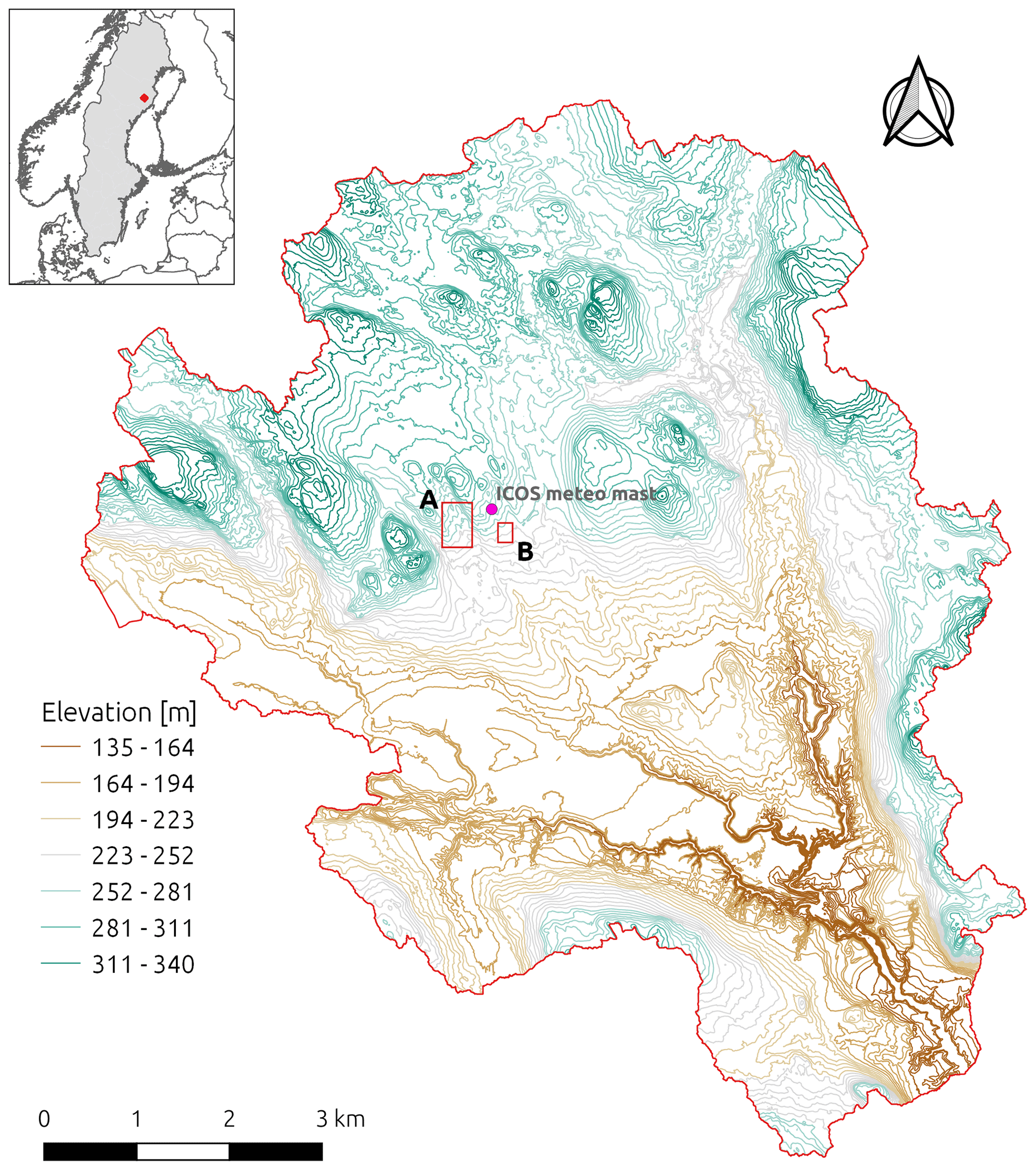
Figure 1The Krycklan catchment and the location of the two study areas where the groundwater wells were installed (red squares) at points A (in C6) and B (S-transect in C2). The location of the ICOS station is marked by a point (north of area B). The inset shows the location in of the Krycklan catchment in northern Sweden. See Fig. 2 for a more detailed map of the study areas. Datum from SWERREF99 TM – EPSG:3006.
3.1 Well network design
The locations for the wells were chosen based on the lidar-derived digital elevation model (DEM), with a closer well spacing in areas where we either expected very stable or very variable flow directions or gradients (Erdbrügger et al., 2021). To allow for the determination of groundwater gradients (i.e., flow directions), the wells were located in triangles of different sizes, namely 5, 10, and 20 m (Fig. 2). In the field, the planned positions of the wells were identified with a handheld GPS and the help of elevation and vegetation maps. Not all wells could be installed as planned. For some locations, the position had to be adjusted due to the presence of trees and big boulders. In addition, the access requirements for the drill rig (see Sect. 3.2) meant that the location of some of the wells had to be moved. However, in most cases, the wells could be installed within 5 m of the pre-determined positions based on the DEM.
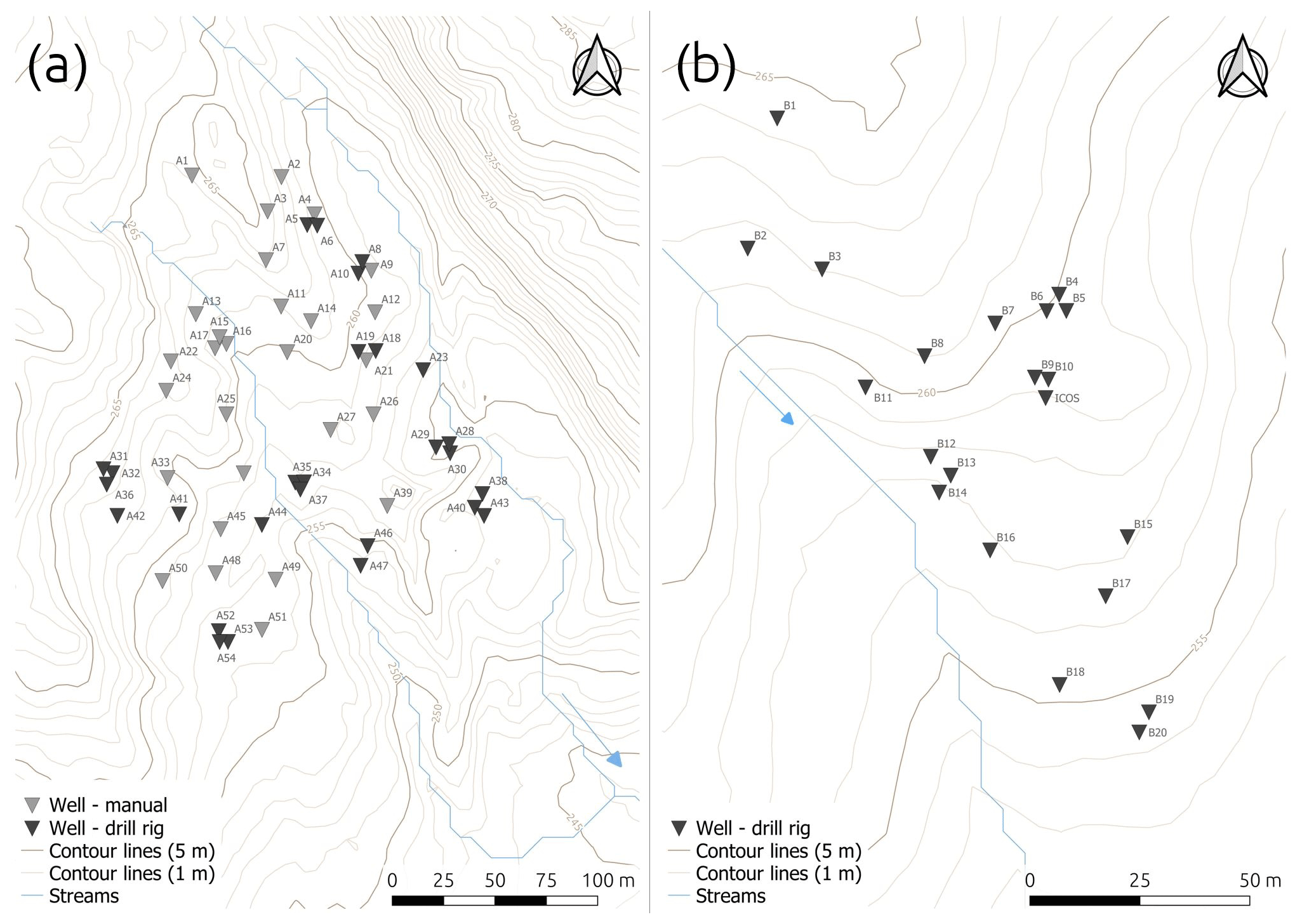
Figure 2Maps of the two study areas, with area A in panel (a) and area B in panel (b). The locations of the 75 wells (triangles) that were either augured by hand (manual; in light gray) or installed by the drill rig (dark gray) are also shown. The letters next to each triangle indicate the name of the well. See Fig. 1 for the location of the two study areas within the Krycklan catchment.
3.2 Well installation
We installed 27 wells with a Cobra petrol-driven drill and breaker between May and October 2018 (all in area A) and 48 wells (27 in area A and 21 in area B) with a drill rig between February and March 2019 (Figs. 2 and 3). The drill rig was used in winter, when the ground was frozen and covered by a thick snowpack, to minimize the impact of the heavy machinery on soil and vegetation. The wells consist of fully screened PVC pipes, with an outer diameter of 5.0 cm and an inner diameter of 3.7 cm. A filter sock was placed over the entire screened length of the pipe to limit the entry of particles into the well.
The required well depths were estimated based on the depth to water index (Murphy et al., 2009), which was calculated based on the DEM but was adjusted based on the groundwater levels observed during installation. Many of the wells needed to be deeper than suggested by the index. For the installations during winter, the required depths were based on the groundwater depths measured in the summer. We tried to install the wells at least 1 m deeper than the lowest observed groundwater level in nearby wells. The target depth could not be reached in some cases due to boulders or other obstacles. As a result, some wells were not sufficiently deep to measure the groundwater level during the driest periods. This was particularly the case for the wells located furthest away from surface waterbodies. The average depth of the wells was 274 cm (standard deviation of 113 cm; range of 57–578 cm). The depth of the wells installed in summer (with a Cobra drill) was generally less (average of 193 cm; range of 57–386 cm) than for the wells installed in winter with the drill rig (average of 316 cm; range of 168–578 cm).
The height of the top of the wells above the ground (i.e., the stick-up) was measured after the installation on three occasions in 2018 and two occasions in 2019. A marker on the pipe ensured that this height was always measured on the same side of the pipe. The position of the well tops may have shifted slightly over the measurement period due to the freezing and thawing of the ground. Soil heave in the Krycklan catchment can be several centimeters over the frost season (Bergsten et al., 2001). We, however, assume that this effect was minor for the wells (and thus the well tops) because the pipes reached well below the average freeze–thaw line, which is located at −19 cm in the Krycklan catchment (Panneer Selvam et al., 2016). Thus, although the relation of the tube top to the soil surface may have changed slightly over time due to soil heave or trampling, we assume that the relation of the well tops to each other remained the same.
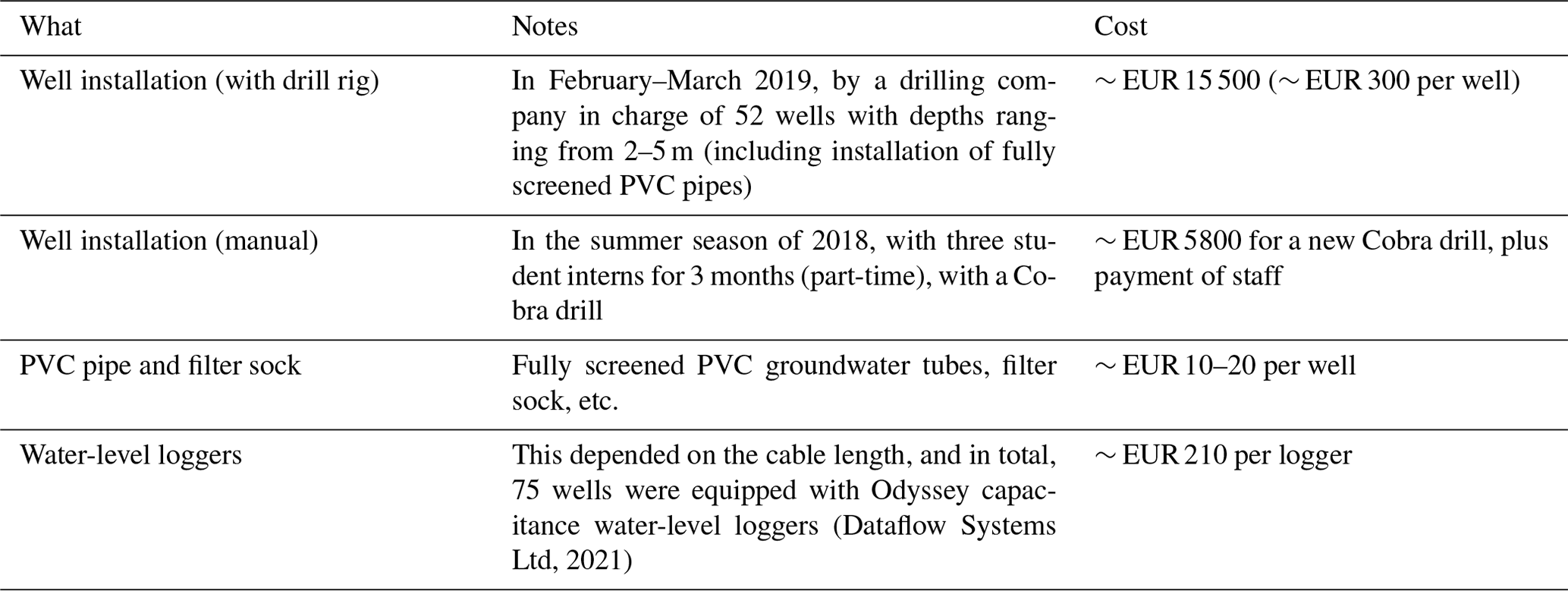
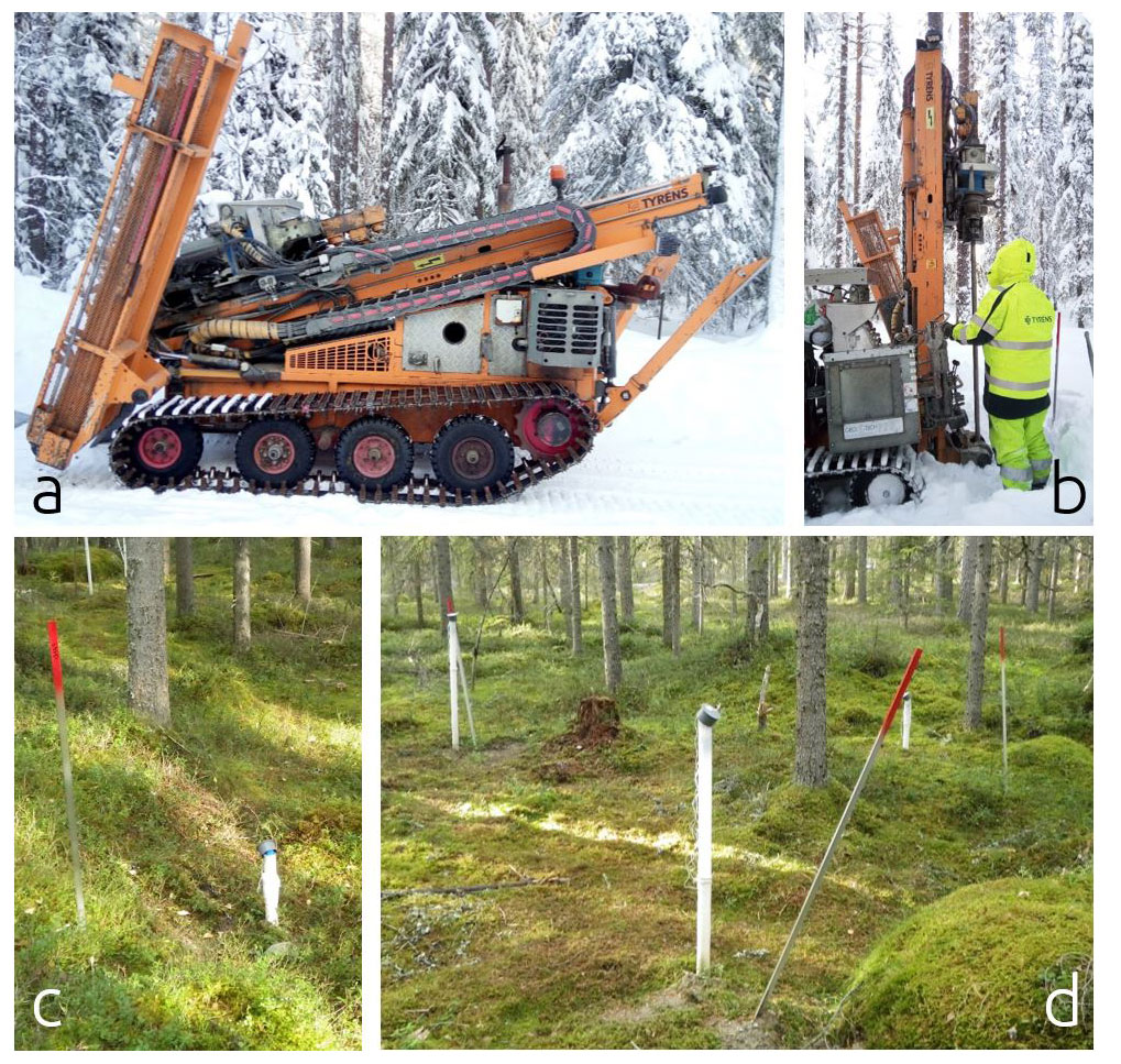
Figure 3(a, b) Well installation in winter 2019. (c, d) Pictures of closely positioned wells that form triangles (length of the pipe above the ground is ∼ 50 cm in panel c and 110 cm in panel d). The gray caps were placed over the loggers for protection. The aluminum poles with the red paint next to the wells were used to determine the location of the wells when snow covered the ground.
3.3 Well georeferencing
After installation, the position of the wells was determined with a high-precision GPS. All wells were scanned with a terrestrial laser scanner (Trimble TX8) in May 2019 to more accurately determine the vertical and horizontal positions relative to each other. About 68 single scans (39 in area A and 29 in area B) were done at a distance of about 20 m. The scan resolution at 30 m from the scanner was one point every 11.3 mm (Trimble Inc., 2017). The generated point clouds were combined into one large point cloud, following the procedure proposed by the Ljungberg's Remote Sensing laboratory at the Swedish University of Agricultural Sciences (Bohlin and Nyström, 2019). The wells were manually identified in the combined point cloud, and the upper end of the tube was taken as the reference point (Fig. 4). The relative positions of the wells are given in the Krycklan_gw_wells.csv file. The registration reports are given in the 2022-020_Erdbruegger-et-al_TLS_registration_area[A/B].rtf files. The complete scan data are available via the Krycklan database (Lindgren, 2021).
The positions of the well tops were exported as an ESRI shapefile. We then used a similarity transformation (only rotations and x and y offsets; no scaling) to georeference the well positions (x and y coordinates only). As orientation points for the similarity transformation, we used the locations of four wells measured in the field with the high-precision GPS. Since the scan was already level in the horizontal direction (using the terrestrial laser scanner (TLS) internal leveling), we adjusted the z offset by the GPS z position of one of the wells to obtain a general offset for all wells. The procedure was carried out separately for the two study areas (A and B; Table 1).

Figure 4Example of the point clouds for manually identified wells. The well (on the right and in the foreground on the left), filter sock, the aluminum pole (in the middle, with the top cut off) marking the well, and surrounding vegetation are clearly visible in the point cloud.
4.1 Dataset structure
The groundwater-level dataset (Dataset 1) consists of two files. One file (2022-020_Erdbruegger-et-al_Krycklan_gw_wells.csv) provides a description of each well, and the other file (2022-020_Erdbruegger-et-al_Krycklan_gw_wells.csv) provides the time series of the actual measurements and the calculated water level in meters above mean sea level (m a.m.s.l.) for each well. See Table B1 for the structure of the groundwater well location data file (2022-020_Erdbruegger-et-al_Krycklan_gw_wells.csv) and a description of the column names. Also see Table B2 for the structure of the groundwater-level data file (2022-020_Erdbruegger-et-al_Krycklan_gw_levels.csv) and a description of the column names of these data files. The measurements and data processing steps to obtain the time series of the groundwater levels are described in the following sections.
4.2 Manual water-level measurements
The distance between the top of the well and the water level (man_level) was manually measured (weekly to bi-weekly) in July, September, and October 2018 and between May and September 2019. On average, the depth to the water level could be manually measured 14 times (range of 0–26). For shallow (< 1 m) groundwater levels, we usually used a bubbler to measure the distance between the top of the well and the water level. When the water level was deeper, we used either a water-level plopper (kluk lod in Swedish) or an acoustic water-level sounder because the bubbler did not work as well under these conditions. For more detailed information on these manual measurements, see Appendix E.
The distance to the water level was noted directly in a spreadsheet and on paper for cross-referencing after the fieldwork. These data were screened visually and checked for plausibility. Data points that deviated strongly from the expected range were double-checked based on field notes, meteorological data, and data from nearby wells. Data entries outside the expected range that could not be confirmed by any other source were classified as outliers. In total, five manual measurements that deviated more than 1 m from the expected value were excluded and are assumed to have been entered incorrectly in the data sheets.
4.3 Continuous water-level measurements
4.3.1 Initial logger calibration, installation, and maintenance
For the continuous water-level measurements, we installed capacitance water-level loggers (Dataflow Systems Pty Ltd, Christchurch, New Zealand) in 74 wells. The length of the cable of the water-level loggers was based on the depth of the well and the expected changes in water level. Although we used loggers with different housing lengths and cable lengths, they all function similarly (see Appendix E). The resolution of the sensors is 0.8 mm (Dataflow Systems Ltd, 2021).
All loggers were calibrated according to the instructions provided by the supplier (Dataflow Systems PTY Limited, 2012) prior to field installation. In short, two points (at 20 and 140 cm from the lower end of the weight at the end of the cable; see Fig. E1) were marked, and the logger was suspended in a sealed PVC pipe filled with water from one of the groundwater wells so that the water reached exactly the mark on the cable. For each position, the raw measurement values were noted after an acclimatization phase of about half a minute or until the values had stabilized. This two-point linear calibration was used to convert the raw sensor values to distances (in cm) above the bottom of the sensor.
The loggers were set to record at a 10 min interval, except in the first measurement week when it was 15 min and in winter 2018/2019 when it was set to 30 min to avoid filling the memory (and overwriting the data) during the winter period. The data were downloaded three or four times during the field season (May to October). Loggers that did not record any data or only recorded data for part of the period were inspected and usually re-installed on the same day or on the following day.
We had to take the loggers out of the wells for the manual water-level measurements. We tried to time this so that it would not coincide with the measurements (i.e., we aimed to do this within the 10 min interval between measurements). When the data were being downloaded, the loggers were inspected visually for any disturbances, such as biofilm or dirt on the cable, kinks, or obstructions and were cleaned when necessary. At this time, we also measured and adjusted the logger string lengths if the groundwater level had fallen, or was expected to fall, below the deepest point of the sensor, or if it was expected to rise above the logger body during snowmelt.
The groundwater level (Log_level_uncorr; in cm) below the top of the well was calculated by subtracting the water level measured by the logger (in cm from the bottom of the logger weight) from the sum of the length of the logger body, cable and weight length, and string length (see Fig. E1). These water-level time series were inspected manually for incongruities. For five wells, the string length information was accidentally not recorded for all periods (after adjustments due to very high or very low water levels in the well), so the groundwater level below the top of the well could not be calculated; these data points were marked (Offset flag; see Sect. 4.4) and can only be used to investigate groundwater-level dynamics but not the actual level.
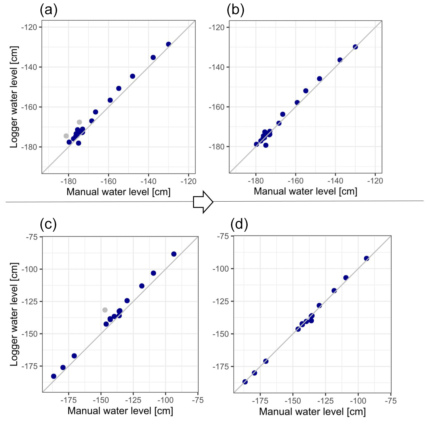
Figure 5Relation between the manual and logger water-level measurements (in cm) below the top of the well before (a, c) and after (b, d) the re-calibration of the logger for well A7 (a, b) and well B18 (c, d). Manual measurements that were identified as outliers are marked in gray (in panels a and c). The correction factor (i.e., intercept) was −1.2 cm for well A7 and −3.9 cm for well B18.
4.3.2 Logger-level data correction (re-calibration)
When analyzing the data, it became apparent that there was a systematic offset between the logger data (Log_level_uncorr) and the manual measurements (man_level; Fig. 5a and c), with the logger-based water levels being systematically higher (i.e., closer to the surface) than the manual measurements. In some cases, they were above the surface, although we only observed flooding for two of the wells (i.e., only for these two wells did we expect the water levels to rise above the ground surface at some point in the year). We deemed the manual measurements more reliable and assumed that the shift was due to a systematic error in the initial calibration of the loggers or calculation of the logged water levels. We can exclude the pipe length (which would have been an individual error for each well) and string length (the shift also appears for loggers that were not attached to strings) as the source of the systematic error and, therefore, assume that the shift was due to a systematic offset in the calibration of the loggers before field deployment.
We corrected the logger data in a two-step process based on the assumption that we only needed to correct the vertical shift in the logger data. We first determined the linear regression between the manual measurements and logger data, using a slope of one. We then defined points more than 5 cm from this initial linear regression as outliers caused by errors in the manual water-level measurements. After excluding these outliers, we determined a new linear regression between the manual measurements and logger-derived water-level data, again with a slope of one, and calculated the offset (see two examples of the correction in Fig. 5). The mean value for this correction (i.e., intercept) was −9.91 cm (standard deviation of 6.74 cm; range of −28.1 to −0.05 cm). We then used this offset (intercept) to correct the logger data. Thus, effectively, we lowered the logger data to match the manual water-level measurements. This fixed the issues with the water levels rising above the surface for all wells for which this was not observed. The data were not corrected for 18 of the 74 wells because there were fewer than two valid manual water-level measurements to calculate the correction (i.e., intercept).
The final absolute groundwater level (Log_level_corr; in m a.s.l.) was calculated by adding the correction factor (intercept) to the uncorrected logger level (log_level_uncor) and the elevation of the well top (Z_abs): Log_level_corr = Z_abs – (Log_level_uncorr+intercept).
4.4 Data flagging
Outliers or discontinuities in the water-level time series were classified into six different categories (Table C1; Fig. 6). This flagging allowed us to keep all data points in the record so that they can be re-evaluated if necessary.

Figure 6Example of a groundwater time series (well A12; May 2019) affected by two pumping events, with the identification of the outliers (black) during the time that the logger was outside the well (while the pumping took place) and the recovery period (green). Water levels below the threshold of 5 cm above the logger end are classified as censored (red).
To download the loggers, take manual water-level measurements, or purge the wells for cleaning and sampling (see description of Dataset 2), the loggers were taken out of the wells. This usually took a short time, and therefore, the loggers were not stopped. Most of the measurements taken during these periods were significantly lower than those taken before or afterwards and are consequently classified as outliers. To find these outliers, we used a filter based on the changes in the water levels. Assuming that groundwater levels generally do not drop abruptly (i.e., the recession is smooth), we used a threshold value of a larger than 10 cm drop in groundwater level within 10 min to find outliers. These outliers were then manually investigated to ensure correct identification.
Data points collected after the re-introduction of the logger into the well after well purging were classified as recovery to mark the time of recovery of the water level within the well. To be sure that equilibrium had been reached, all data points within 12 h after the re-insertion of the logger to the well were classified as recovery. Where the recovery time appeared to exceed the 12 h time span, we extended the classification to 24 h after the re-introduction of the logger.
When the groundwater level was close to the weight at the end of the sensor cable, the recorded data often showed sudden jumps, suggesting a low accuracy of the measurements. To eliminate this problem and the problem of standing water in the very bottom of the well (which was not screened), we classified all points that were less than 5 cm above the logger end as censored.
For 5 of the 74 wells (A21, A9, A4, B1, and B6), we observed a continuous drop in the water level between 21 and 30 April 2019 (see examples in Fig. 7). We expect the groundwater level to rise rather than drop for this peak snowmelt period. The start of the drop in the water level differed for the wells, but it ended suddenly for all five wells on 30 April 2019, when the loggers were removed from the wells to download the data. After the re-introduction of the loggers in the wells, the measured water levels were several centimeters higher than before. The logger string or tube lengths were not adjusted during this period, and the sudden change in the recorded water level cannot be related to errors in these measurements. The wells for which this strange behavior was observed were not located in one region or characterized by a particular topographic position either. These were all located close to other groundwater wells (within ∼ 5 m), for which we did not observe such a change. Therefore, the data from these wells during this period are flagged as strange. Because the recorded time series after the re-introduction of the loggers to the well seems to agree with the water levels observed in the days before the sudden drop, we expect that the lowering of the electrical conductivity (EC) of the water in the wells due to the infiltration of low EC meltwater caused this change. Odyssey water-level logger recordings can be sensitive to a large change in EC (Larson and Runyan, 2009). It is most probably the case that the removal of the logger from the well and its re-introduction stirred the water inside the wells and led to the mixing of the meltwater and older groundwater. The alternative explanation of a film (biological or other) on the cables does not correspond with our field notes. Only in two cases was a film observed on the sensor cable, but for these sensors, the logged values seem to be normal during this period.

Figure 7Examples of strange drops in the measured water level during the 2019 spring melt period for two wells (well A4 in panel a and well A21 in panel b).
Table 2Description of groundwater sampling data (file 2022-020_Erdbruegger-et-al_Krycklan_sampling.csv).
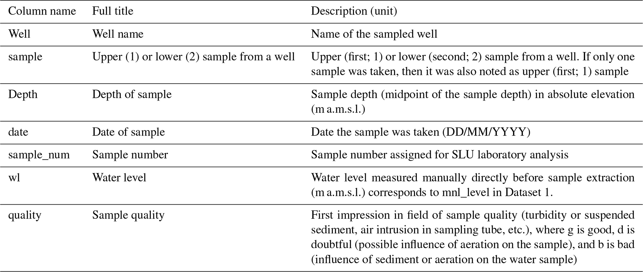

Figure 8Precipitation (first plot; blue bars), temperature (daily average; second plot; red line), and classified groundwater levels for two wells (A12 in the third plot; B18 in the fourth plot) between June 2019 and September 2020. See Table C1 for further information on the classification of the data points.
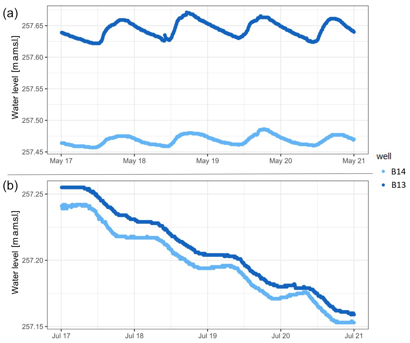
Figure 9Example time series showing diurnal variations in groundwater levels for two wells during the late snowmelt period in May 2020 (a) and the summer (July 2020) when diurnal variations are caused by evapotranspiration (b).
5.1 Dataset structure
In the summer of 2019, a groundwater sampling campaign was undertaken to obtain spatially distributed information on groundwater chemistry. The resulting groundwater chemistry dataset (Dataset 2) consists of four files. One file (Krycklan_sampling.csv) provides a description of each sample (Table 2) and another one (Krycklan_chemistry.csv) gives the laboratory results for each sample (see Table D1 for a description of the file structure). The third file contains the field protocol (Field_protocol.csv), and the fourth file (Lab_analysis_description.pdf) provides additional details on the laboratory analyses. The sampling and data analyses are described in more detail in the following sections.
5.2 Sampling
The groundwater sampling was done between 19 and 31 July 2019. Total precipitation during the sampling period in July was relatively low (28 mm in total; max daily precipitation 13 mm). The sampling procedure and field protocol used for the campaign followed the Svartberget research station and Swedish University of Agricultural Sciences (SLU) standard procedure for groundwater sampling (see also the 2022-020_Erdbruegger-et-al_Field_protocol.csv-file). To ensure that the water samples were representative of the local groundwater, we did two rounds of purging with a peristaltic pump (see Fig. F1) between the middle (shortly after peak snowmelt) and the end of May 2019 (when groundwater levels were generally lower than for the first round). During both rounds, the wells were either pumped dry or at least 3 times the well volume (see Appendix F) was pumped out to ensure full replacement of the well water with fresh groundwater. The pumping also removed the sediment and other particles from the wells.
A custom-made straddle packer system with inflatable rubber tubes (see Appendix F; Fig. F2) allowed us to isolate a specific part of the well and sample water from a roughly 25 cm long interval. We aimed to obtain two samples per well, with one sample just below the groundwater table (which corresponds to the uppermost portion of the groundwater at the respective location) and another sample from the deepest part of the well. Because many wells were shallow and groundwater levels were low at the end of July, there was insufficient water for two samples for many wells. In these cases, we took only one water sample from the deepest point of the well.
The pumping was done slowly (regulated manually) to not draw water from above, allow for recharge, and avoid excessive aeration of the samples. However, in some cases, the recharge of the wells was so slow that even the lowest pumping rate was too high, and the water level in the well dropped, or the well was pumped dry and aeration of the samples took place. When aeration occurred, it was noted in the sampling protocol as a qualitative indication that the sample quality might be doubtful (d) or even bad (b; see Table 2). Prior to taking the actual sample, the tubes were flushed with ∼ 2 L of well water to reduce cross-contamination of samples. The sample bottles were rinsed three times before filling them to the top without air bubbles. Additionally, we measured the electrical conductivity (EC) and pH in the field with a pH/Cond 3320 sensor (Xylem Analytics Germany Sales GmbH & Co. KG).
5.3 Lab analyses
The samples were analyzed for EC, pH, absorbance at 254, 365, 420, and 436 nm, anion (F, Cl, and S-SO4) concentrations, nutrient (P-PO4, N-NH4, and N-NO3) concentrations, and stable isotopes (δ18O and δ2H) in the laboratory of SLU, Sweden. The cation (Na, NH4, K, Mg, and Ca) concentrations were analyzed at the Hydrogeological Laboratory of the TU Bergakademie Freiberg, Germany. A detailed description of the lab procedures is given in the file 2022-020_Erdbruegger-et-al_Lab_analysis_description.docx.
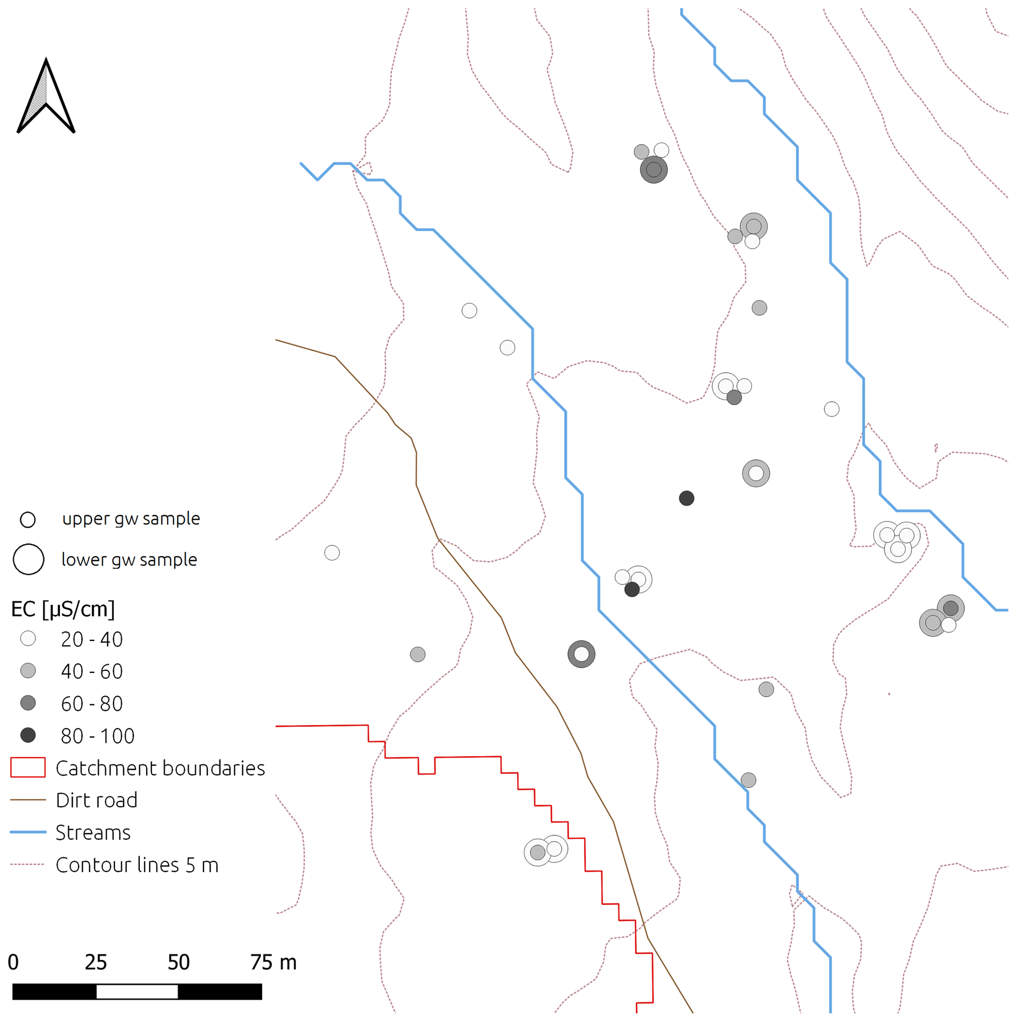
Figure 10Map of the electric conductivity (EC) of the groundwater samples taken near the water table (small circle; upper groundwater sample) and the bottom of the well (larger circle; lower groundwater sample) for the wells in study area A (also known as the C6 catchment). Where two circles are shown, the outer circle represents the groundwater sample taken from the bottom of the well and the inner circle the groundwater taken near the water table.
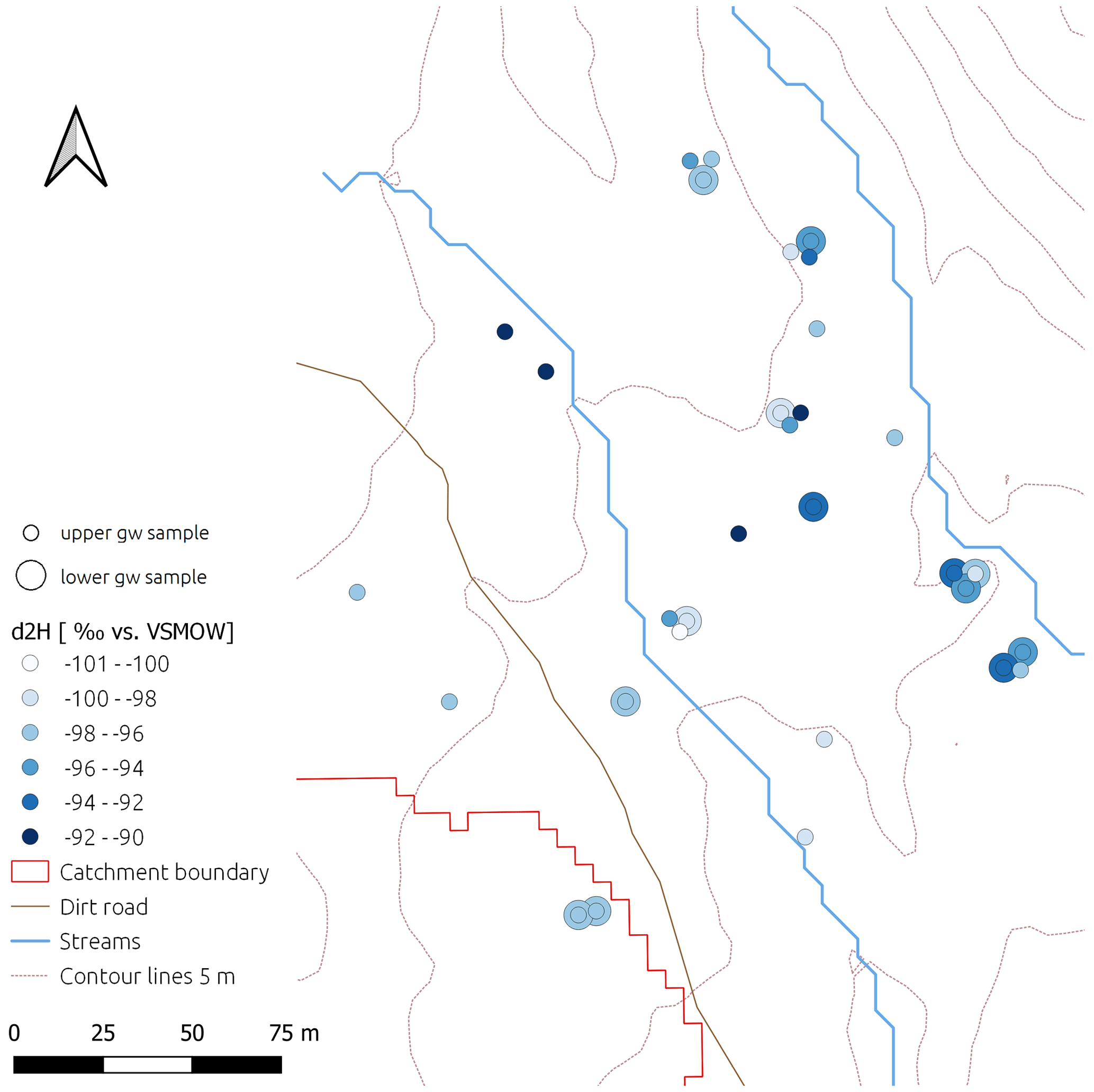
Figure 11Map of δ2H of the groundwater samples taken near the water table (small circle; upper groundwater sample) and the bottom of the well (larger circle; lower groundwater sample) for the wells in study area A (also known as the C6 catchment). Where two circles are shown, the outer circle represents the groundwater sample taken from the bottom of the well and the inner circle the groundwater taken near the water table.
6.1 Groundwater-level data
Figure 8 shows the groundwater-level time series for two selected wells (A12 and B18) and highlights the quick response to snowmelt and rainfall events. Thanks to the relatively high resolution of the groundwater data, the immediate response of groundwater levels to specific rainfall events is clear. Interesting dynamics like daily groundwater-level variations due to snowmelt, with peak water levels occurring during the early evening (see examples in Fig. 9a) and due to evapotranspiration with groundwater levels dropping during the day and stabilizing at night (see examples in Fig. 9b) can also be observed for most wells (cf.Kirchner et al., 2020).
6.2 Groundwater chemistry
The concentrations of the anions, cations, and nutrients in the groundwater are comparable to those reported from other measurements in the Krycklan catchment (e.g., Kolbe et al., 2020; Laudon et al., 2013, 2021), but the spatial variation in the concentrations was large (cf. Kiewiet et al., 2020), with the coefficient of variation ranging from 2.5 % (for δ18O) to 239 % (for F; see examples in Figs. 10 and 11). The concentrations for the lower groundwater samples differed from those of the upper groundwater samples for most locations (e.g., Fig. 10), but no clear trends could be identified. The isotopic composition of the groundwater was also variable, with the δ2H, for example, varying by 12.5 ‰ for the groundwater samples taken near the groundwater table (Fig. 11).
Datasets 1 and 2 can both be accessed and downloaded via https://doi.org/10.5880/fidgeo.2022.020 (Erdbrügger et al., 2022). The zip-compressed folder (2022-020_Erdbruegger-et-al_Krycklan_Groundwater_levels_sampling.zip) includes all the files listed in Table A2. A brief description of the data and information on licensing and the format of the tabular data is available from 2022-020_Erdbruegger-et-al_data-description.pdf (available separately and also located within the zip folder).
The datasets presented in this paper can be used to investigate the spatiotemporal dynamics of shallow groundwater and to test hydrological models or upscaling approaches. These data can be used in other studies in the Krycklan catchment to better understand its hydrological functioning or geochemical or ecological processes. The highly instrumented sites within the Krycklan catchment provide unique opportunities to study groundwater dynamics. The potential findings are relevant for other boreal catchments. The wells are still in place and accessible. Thus, there is the possibility for continued groundwater-level measurements and repeated sampling.
Table A1Selected catchment and hillslope-scale studies with a large number of shallow groundwater-level measurements and reported well densities (number of wells per hectare).

Table A2Name and short description of the data files included in the two datasets.
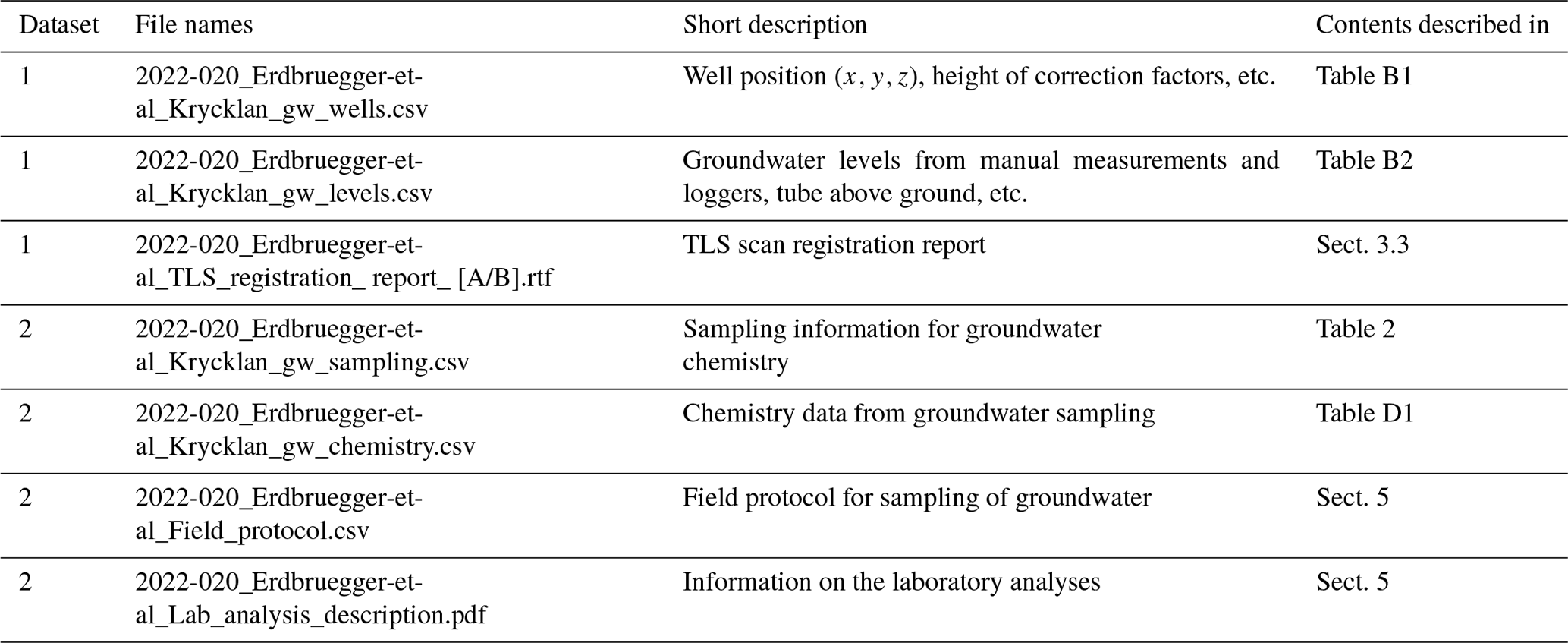
Table B1Structure of the groundwater well location data file (2022-020_Erdbruegger-et-al_Krycklan_gw_wells.csv) and description of the column names.
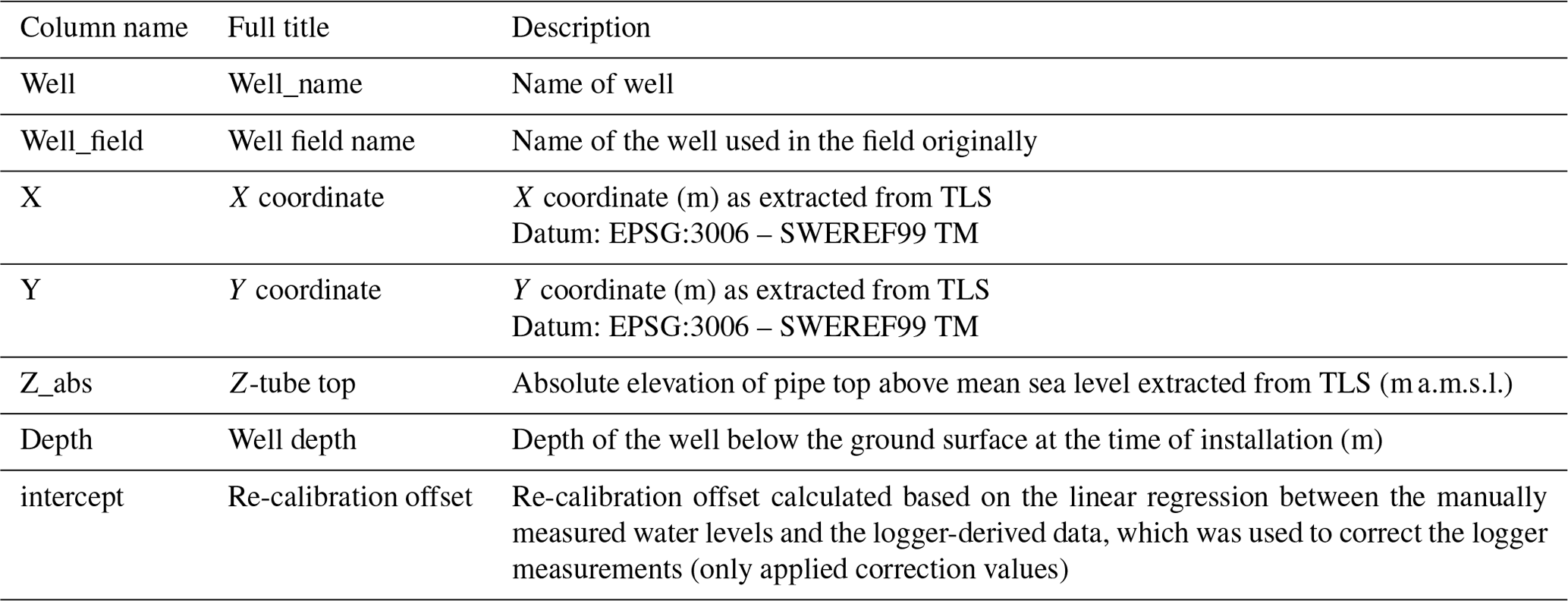
Table B2Structure of the groundwater-level data file (2022-020_Erdbruegger-et-al_Krycklan_gw_levels.csv) and description of the column names.
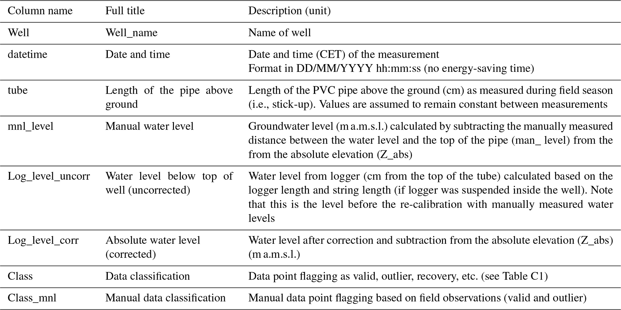
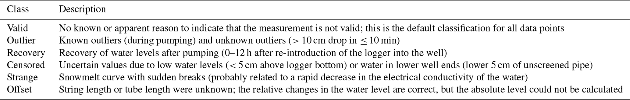
Table D1Description of groundwater chemistry data (file 2022-020_Erdbruegger-et-al_Krycklan_chemistry.csv). See the Lab_analysis_description.pdf file for more information on the laboratory analyses.
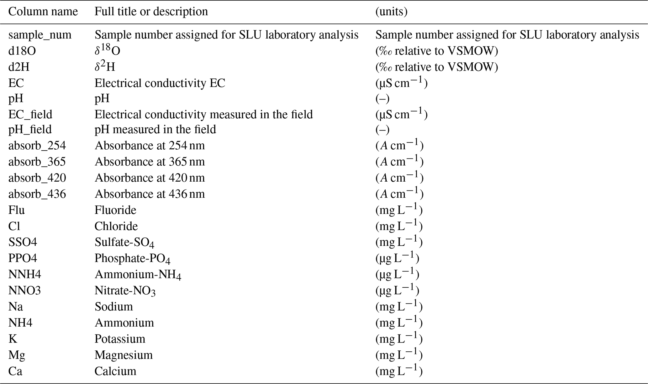
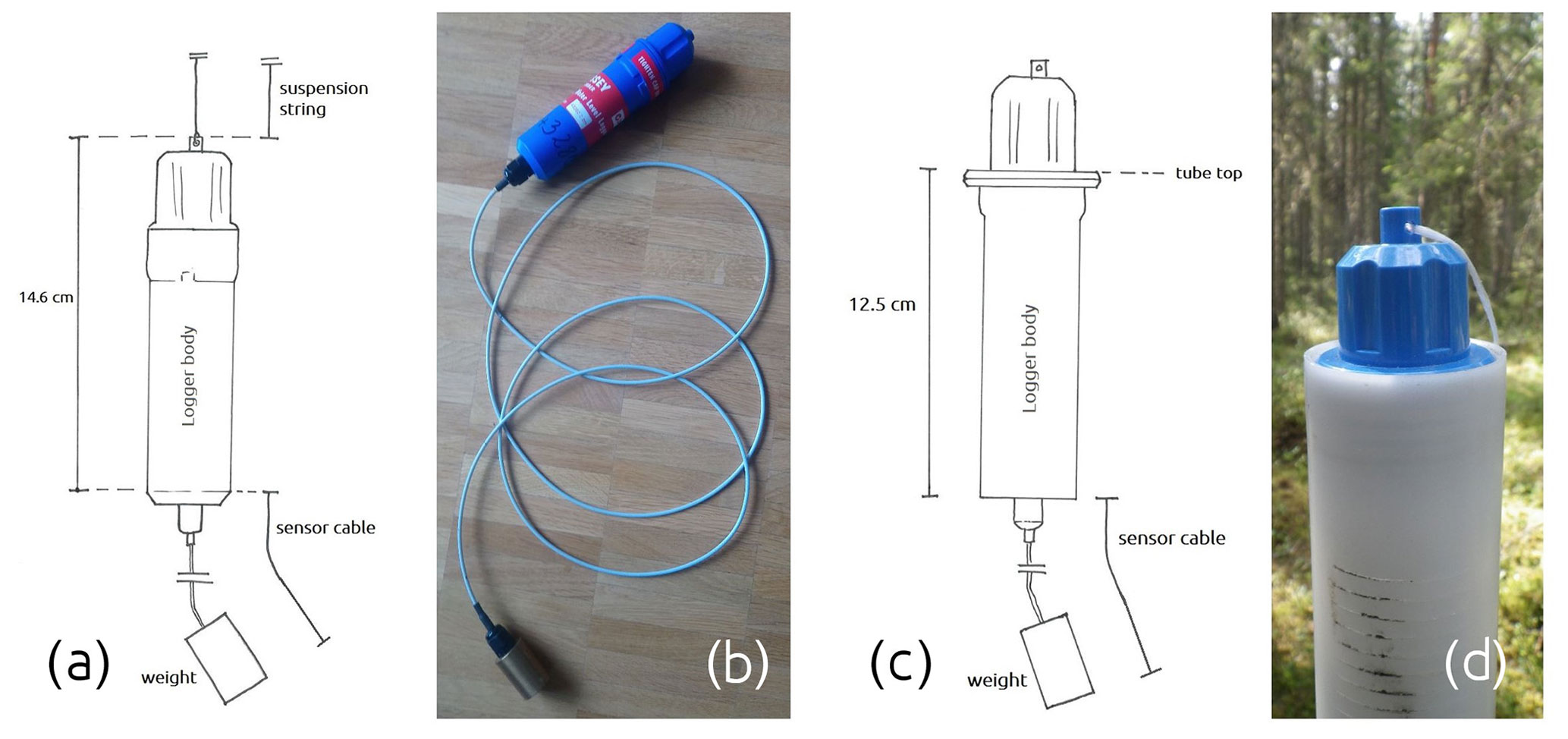
Figure E1Odyssey water-level loggers and the lengths of the logger body and cable for the 2012 Odyssey water-level sensor (a, b), the 2019 Odyssey water-level sensor (c), and the 2019 sensor installed in a well tube (d). Note that the drawings are not to scale.
E1 Manual water-level measurements
We used three different methods to measure the depth between the top of the well and the water level, namely a bubbler, a water-level plopper (kluk lod), and an acoustic water-level sounder. The so-called bubbler consists of a rigid tube connected to flexible tubing. In our case, we used a 1 m long metal tube with a ∼ 5 mm diameter connected to flexible rubber tubing. The metal tube was inserted into the well and air was blown into the flexible tube. The water level in the well was determined based on the change in the sounds once the metal tube reached the water surface (i.e., as soon as one could hear a bubbling noise). This method worked best for shallow groundwater levels since the sound was difficult to discern when the water level was deeper (this also applied to noisy circumstances such as strong winds). Because the water can be blown out of the well when blowing too strongly, leading to a slightly deeper groundwater level, we carefully approached the groundwater surface from above and provided only moderate pressure.
A water-level plopper consists of a small metal cylinder attached to the tip of a measuring tape. It is lowered into a well and produces a plopping sound when the cylinder hits the water surface. When the water level was deep (> 3 m), the sound was sometimes not audible. Also, for shallow groundwater levels, it often took several tries and plopping sounds to determine the exact depth to the water level because it required enough momentum for the cylinder to produce a sufficiently distinguishable sound. The electronic water-level meter or (acoustic) water-level sounder emits a sound upon contact with water. In addition, a light switches on. The sensor at the tip of the tape or meter has an open electrical circuit and closes when it is in contact with water because of the much lower resistivity of water than air. Because the groundwater in the Krycklan area has a relatively low electric conductivity (mean EC from the surveys 48.6 µS cm)−1, the electronic water-level meter sometimes failed and indicated the water surface only after being submerged for about half a meter. The problem was solved after purging the wells or stirring the water in the wells. The low EC in some wells may have originated from the snowmelt water that did not drain or mix much with the other groundwater in the well.
E2 Continuous water-level measurements
We used Odyssey water-level loggers for the continuous water-level measurements. These capacitance sensors are based on the difference in the dielectric constants of water and air. The weight at the end of a cable serves as one capacitance plate and the cable as the second. A change in the area of the second capacitance plate (i.e., the cable in contact with the water) results in a change in the signal. For more information on capacitance sensors, see Larson and Runyan, 2009, Dataflow Systems PTY Limited, 2012, and Guaraglia and Pousa, 2014. We deployed two generations of the same type of loggers, which differ in their dimensions (Fig. E1a and c). The new logger bodies (from 2019) are larger and do not fit completely into the well pipes (see Fig. E1b and d).
The water used for the calibration was taken from a groundwater well to account for local water chemistry (as this was shown to be a potential error source by Larson and Runyan, 2009) and thus to minimize errors in the calibration. Other error sources identified by Larson and Runyan (2009), like the potential for a biofilm to build up on cable and counterweight of the loggers, were minimized by cleaning the cables and weights with a cloth during logger read-outs. The building of films varied strongly between wells but did not appear to have an identifiable impact on the data, and therefore, we did not correct for this.
Since the loggers do not show the remaining battery power, it is relatively difficult to predict when they run out of power. Although a rough estimate says the batteries last for about 18 months, this time can vary considerably with environmental factors and is much shorter during low temperatures. This resulted in incomplete time series for some wells (see Table G1 in Appendix G).
The well purging and subsequent sampling was done using two peristaltic pumps (see Fig. F1). The volume of water that needed to be pumped from the well during purging was calculated based on the volume of water inside the well and multiplied by a factor of 3 to ensure the recharge of fresh groundwater, as follows:
where the Vpump is the volume to be pumped, dwell is the inner well diameter (3.7 cm for our wells), Lwell is the well depth (from tube top), and dgw is the depth from the well top to the water level.
In some cases, recharge into the well was very slow, and in these cases, we would stop the purging when the well ran dry (i.e., before Vpump was reached). All wells (with water in them) were purged twice within the space of 2 weeks. After the second purging round (31 May 2019) and before the sampling campaign started (1 July 2019), precipitation was 68.4 mm.
For the groundwater sampling, we used a custom-made packer system (Fig. F2) that could seal off the access to water below and above the part where the sample would be taken. This allowed sampling at discrete depths. Markers on the tube of the packer system allowed the determination of the sample depth. The packer was designed to sample up to a depth of 6 m. Since the sample opening is located above the lowest end of the packer, a minimum water level of 40 cm inside the well was necessary to take a sample with the packer system.
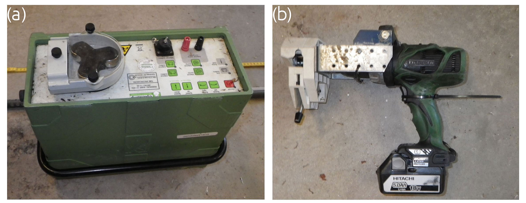
Figure F1Photo of a peristaltic pump (a). Peristaltic pump mounted on a drill (b) used for purging the wells.

Figure F2Photo of the custom-made straddle packer system with two inflatable parts to isolate specific depths in the wells and to pump water from a specific depth (a). The upper part and tubing system (pumping tube and two air tubes to inflate the flexible tube parts) of the packer system (b). The yellow arrows in panel (a) indicate to the inflatable packer system parts that sealed off (i.e., isolated) water above and below the selected sample depth.
Table G1Summary of the recorded water-level data per well and the manual measurements for each well. The summary statistics (mean, median, minimum, and maximum) were only calculated over the valid data points. Note that for some wells (e.g., A45 and A50) the number of valid data points is very small because the well was dry for most of the study period or the data were flagged as censored data. The number of outliers include the number of times that the well was dry as well.

JE, IvM, JS, and KB designed the experiments. JE led the installation of the wells, field measurements, recording of the water levels, and sampling. JE prepared the paper and data files, with contributions from all co-authors.
The contact author has declared that none of the authors has any competing interests.
Publisher's note: Copernicus Publications remains neutral with regard to jurisdictional claims in published maps and institutional affiliations.
We thank everyone involved in the installation and maintenance of the wells, especially Tommy Andersson, Alexandre Constan, Olivier Dulouard, Corentin Leprince, Johannes Larson, Ola Olafson, Paul Pister, Viktor Sjöblom, Jacob Smeds, Johannes Tiwari, and Jean-Thomas Wenner. We also thank SITES and SLU Umeå for granting access to the area and research station and providing field equipment. Furthermore, we thank Hjalmar Laudon, Ida Manfredson, Charlotta Erefur, and the entire Svartberget field research station crew for all the help with logistics and moral support during the fieldwork.
This research has been supported by the University of Zurich. The installation of the groundwater wells was made possible by funding from SKB (Svensk Kärnbränslehantering AB) and the SLU Excellence award to Hjalmar Laudon.
This paper was edited by Hanqin Tian and reviewed by Christophe Hissler and one anonymous referee.
Bachmair, S., Weiler, M., and Troch, P. A.: Intercomparing hillslope hydrological dynamics: Spatio-temporal variability and vegetation cover effects, Water Resour. Res., 48, 1–18, https://doi.org/10.1029/2011WR011196, 2012.
Bergsten, U., Goulet, F., Lundmark, T., and Ottosson Löfvenius, M.: Frost heaving in a boreal soil in relation to soil scarification and snow cover, Can. J. Forest Res., 31, 1084–1092, https://doi.org/10.1139/x01-042, 2001.
Beven, K. J. and Kirkby, M. J.: A physically based, variable contributing area model of basin hydrology, Hydrol. Sci. Bull., 24, 43–69, https://doi.org/10.1080/02626667909491834, 1979.
Bishop, K., Seibert, J., Nyberg, L., and Rodhe, A.: Water storage in a till catchment. II: Implications of transmissivity feedback for flow paths and turnover times, Hydrol. Process., 25, 3950–3959, https://doi.org/10.1002/hyp.8355, 2011.
Bishop, K. H., Grip, H., and O'Neill, A.: The origins of acid runoff in a hillslope during storm events, J. Hydrol., 116, 35–61, Available from: https://doi.org/10.1016/0022-1694(90)90114-D, 1990.
Bohlin, J. and Nyström, M.: Terrestrial laser scanning – Postprocessing a multiscan using 230 mm balls on the tripods, Ljungbergslaboratoriet – SLU, http://www.rslab.se/terrestrial-laser-scanning/#postprocessingGeoreferencing, last access: 5 November 2019.
Bonanno, E., Blöschl, G., and Klaus, J.: Flow directions of stream-groundwater exchange in a headwater catchment during the hydrologic year Running head: Stream-groundwater exchange during the hydrologic year, Hydrol. Process., 35, 1–18, https://doi.org/10.1002/hyp.14310, 2021.
Condon, L. E. and Maxwell, R. M.: Water Resources Research, Water Resour. Res., 51, 6602–6621, https://doi.org/10.1111/j.1752-1688.1969.tb04897.x, 2015.
Covino, T. P. and McGlynn, B. L.: Stream gains and losses across a mountain-to-valley transition: Impacts on watershed hydrology and stream water chemistry, Water Resour. Res., 43, 1–14, https://doi.org/10.1029/2006WR005544, 2007.
Dataflow Systems Ltd: Odyssey Capacitance Water Level Logger, http://odysseydatarecording.com/index.php?route=product/product&path=59&product_id=50 (last access: 1 April 2022), 2021.
Dataflow Systems PTY Limited: Technical Handbook for Odyssey Data Logger, Christchurch, New Zealand, 2012.
Doering, M., Uehlinger, U., Rotach, A., Schlaepfer, D. R., and Tockner, K.: Ecosystem expansion and contraction dynamics along a large Alpine alluvial corridor (Tagliamento River, Northeast Italy), Earth Surf. Proc. Land., 32, 1693–1704, https://doi.org/10.1002/esp.1594, 2007.
Eklöf, K., Kraus, A., Futter, M., Schelker, J., Meili, M., Boyer, E. W., and Bishop, K.: Parsimonious Model for Simulating Total Mercury and Methylmercury in Boreal Streams Based on Riparian Flow Paths and Seasonality, Environ. Sci. Technol., 49, 7851–7859, https://doi.org/10.1021/acs.est.5b00852, 2015.
Erdbrügger, J., van Meerveld, I., Bishop, K., and Seibert, J.: Effect of DEM-smoothing and -aggregation on topographically-based flow directions and catchment boundaries, J. Hydrol., 602, 126717, https://doi.org/10.1016/j.jhydrol.2021.126717, 2021.
Erdbrügger, J., van Meerveld, I., Seibert, J., and Bishop, K.: Shallow groundwater level time series and groundwater chemistry survey data from Krycklan catchment, GFZ Data Services [data set], https://doi.org/10.5880/fidgeo.2022.020, 2022.
Fan, Y.: Are catchments leaky?, WIREs Water, 6, 1–25, https://doi.org/10.1002/wat2.1386, 2019.
Gabrielli, C. P. and Mcdonnell, J. J.: An inexpensive and portable drill rig for bedrock groundwater studies in headwater catchments, Hydrol. Process., 26, 622–632, https://doi.org/10.1002/hyp.8212, 2012.
Guaraglia, D. O. and Pousa, J. L.: Water Level and Groundwater Flow Measurements, in: Introduction to Modern Instrumentation For Hydraulics and Environmental Sciences, De Gruyter, Berlin, Boston, ISBN 9783110401721, 2014.
Haitjema, H. M. and Mitchell-Bruker, S.: Are water tables a subdued replica of the topography?, Ground Water, 43, 781–786, https://doi.org/10.1111/j.1745-6584.2005.00090.x, 2005.
Haught, D. R. W. and van Meerveld, H. J.: Spatial variation in transient water table responses: differences between an upper and lower hillslope zone, Hydrol. Process., 25, 3866–3877, https://doi.org/10.1002/hyp.8354, 2011.
ICOS: Svartberget, https://www.icos-sweden.se/Svartberget (last access: 1 April 2022) 2021.
Ivarsson, H.: Glacial dynamics and till genesis in hilly terrain: A study in the Tallträsk area, central-northern Sweden, doctoral thesis, Umeå University, Department of Ecology and Environmental Science, Umeå, Sweden, ISBN 91-7264-377-2, 2007.
Ivarsson, H. and Johnsson, T.: Stratigraphy of the Quaternary deposits in the Nyänges drainage area, within the Svarbergets forest experimental area and a general geomorphological description of the Vindeln region, Svartbergets och Kulbäckslidens försökparker, Umeå University, ISSN 0280-4328, Umeå, Sweden, 1988.
Jencso, K. G., McGlynn, B. L., Gooseff, M. N., Wondzell, S. M., Bencala, K. E. and Marshall, L. A.: Hydrologic connectivity between landscapes and streams: Transferring reach- and plot-scale understanding to the catchment scale, Water Resour. Res., 45, 1–16, https://doi.org/10.1029/2008WR007225, 2009.
Jutebring Sterte, E.: Integrated Hydrologic Flow Characterization of the Krycklan Catchment, KTH Royal Institute of Technology Architecture, thesis, TRITA LWR Degree Project, ISSN 1651-064X, KTH, Stockholm, Sweden, 2016.
Kiewiet, L., Freyberg, J., and Meerveld, H. J. (Ilja): Spatiotemporal variability in hydrochemistry of shallow groundwater in a small pre-alpine catchment: The importance of landscape elements, Hydrol. Process., 33, 2502–2522, https://doi.org/10.1002/hyp.13517, 2019.
Kiewiet, L., van Meerveld, I., Stähli, M., and Seibert, J.: Do stream water solute concentrations reflect when connectivity occurs in a small, pre-Alpine headwater catchment?, Hydrol. Earth Syst. Sci., 24, 3381–3398, https://doi.org/10.5194/hess-24-3381-2020, 2020.
Kirchner, J. W., Godsey, S. E., Solomon, M., Osterhuber, R., McConnell, J. R., and Penna, D.: The pulse of a montane ecosystem: coupling between daily cycles in solar flux, snowmelt, transpiration, groundwater, and streamflow at Sagehen Creek and Independence Creek, Sierra Nevada, USA, Hydrol. Earth Syst. Sci., 24, 5095–5123, https://doi.org/10.5194/hess-24-5095-2020, 2020.
Kolbe, T., Marçais, J., de Dreuzy, J. R., Labasque, T., and Bishop, K.: Lagged rejuvenation of groundwater indicates internal flow structures and hydrological connectivity, Hydrol. Process., 34, 2176–2189, https://doi.org/10.1002/hyp.13753, 2020.
Larson, P. and Runyan, C.: Evaluation of a Capacitance Water Level Recorder and Calibration Methods in an Urban Environment, CUERE Tech. Memo, (September), 36, http://www.umbc.edu/cuere/BaltimoreWTB/pdf/TM_2009_003.pdf (last access: 1 April 2022), 2009.
Laudon, H., Berggren, M., Anneli, A., Buffam, I., Bishop, K., Grabs, T., Jansson, M., and Ko, S.: Patterns and Dynamics of Dissolved Organic Carbon (DOC) in Boreal Streams: The Role of Processes, Connectivity, and Scaling, Ecosystems, 14, 880–893, https://doi.org/10.1007/s10021-011-9452-8, 2011.
Laudon, H., Taberman, I., Ågren, A., Futter, M., Ottosson-Löfvenius, M., and Bishop, K.: The Krycklan Catchment Study – A flagship infrastructure for hydrology, biogeochemistry, and climate research in the boreal landscape, Water Resour. Res., 49, 7154–7158, https://doi.org/10.1002/wrcr.20520, 2013.
Laudon, H., Hasselquist, E. M., Peichl, M., Lindgren, K., Sponseller, R., Lidman, F., Kuglerová, L., Hasselquist, N. J., Bishop, K., Nilsson, M. B., and Ågren, A. M.: Northern landscapes in transition: Evidence, approach and ways forward using the Krycklan Catchment Study, Hydrol. Process., 35, 1–15, https://doi.org/10.1002/hyp.14170, 2021.
Leach, J. A., Lidberg, W., Kuglerová, L., Peralta-Tapia, A., Ågren, A., and Laudon, H.: Evaluating topography-based predictions of shallow lateral groundwater discharge zones for a boreal lake-stream system, Water Resour. Res., 53, 5420–5437, https://doi.org/10.1002/2016WR019804, 2017.
Ledesma, J. L. J., Futter, M. N., Blackburn, M., Lidman, F., Grabs, T., Sponseller, R. A., Laudon, H., Bishop, K. H., and Köhler, S. J.: Towards an Improved Conceptualization of Riparian Zones in Boreal Forest Headwaters, Ecosystems, 21, 297–315, https://doi.org/10.1007/s10021-017-0149-5, 2018.
Lindgren, K.: The Krycklan Infrastructure, https://www.slu.se/en/departments/field-based-forest-research/experimental-forests/vindeln-experimental-forests/krycklan/infrastructure/ (last access: 1 April 2022), 2021.
Lyon, S. W., Nathanson, M., Spans, A., Grabs, T., Laudon, H., Temnerud, J., Bishop, K. H., and Seibert, J.: Specific discharge variability in a boreal landscape, Water Resour. Res., 48, 1–13, https://doi.org/10.1029/2011WR011073, 2012.
Moore, R. D. and Thompson, J. C.: Are water table variations in a shallow forest soil consistent with the TOPMODEL concept?, Water Resour. Res., 32, 663–669, https://doi.org/10.1029/95WR03487, 1996.
Munthe, J. and Hultberg, H.: Mercury and methylmercury in runoff from a forested catchment – Concentrations, fluxes, and their response to manipulations, Water Air Soil Pollut. Focus, 4, 607–618, https://doi.org/10.1023/B:WAFO.0000028381.04393.ed, 2004.
Murphy, P. N. C., Ogilvie, J., and Arp, P.: Topographic modelling of soil moisture conditions: A comparison and verification of two models, Eur. J. Soil Sci., 60, 94–109, https://doi.org/10.1111/j.1365-2389.2008.01094.x, 2009.
Myrabø, S.: Temporal and spatial scale of response area and groundwater variation in till, Hydrol. Process., 11, 1861–1880, https://doi.org/10.1002/(sici)1099-1085(199711)11:14<1861::aid-hyp535>3.0.co;2-p, 1997.
Panneer Selvam, B., Laudon, H., Guillemette, F., and Berggren, M.: Influence of soil frost on the character and degradability of dissolved organic carbon in boreal forest soils, J. Geophys. Res.-Biogeo., 121, 829–840, https://doi.org/10.1002/2015JG003228, 2016.
Payn, R. A., Gooseff, M. N., McGlynn, B. L., Bencala, K. E., and Wondzell, S. M.: Channel water balance and exchange with subsurface flow along a mountain headwater stream in Montana, United States, Water Resour. Res., 45, W11427, https://doi.org/10.1029/2008WR007644, 2009.
Penna, D. and van Meerveld, H. J.: Spatial variability in the isotopic composition of water in small catchments and its effect on hydrograph separation, Wires Water, 6, 6:e1367, https://doi.org/10.1002/wat2.1367, 2019.
Ploum, S. W., Laudon, H., Peralta-Tapia, A., and Kuglerová, L.: Are dissolved organic carbon concentrations in riparian groundwater linked to hydrological pathways in the boreal forest?, Hydrol. Earth Syst. Sci., 24, 1709–1720, https://doi.org/10.5194/hess-24-1709-2020, 2020.
Rau, G. C., Post, V. E. A., Shanafield, M., Krekeler, T., Banks, E. W., and Blum, P.: Error in hydraulic head and gradient time-series measurements: a quantitative appraisal, Hydrol. Earth Syst. Sci., 23, 3603–3629, https://doi.org/10.5194/hess-23-3603-2019, 2019.
Retike, I., Bikše, J., Kalvâns, A., Dçliòa, A., Avotniece, Z., Zaadnoordijk, W. J., Jemeljanova, M., Popovs, K., Babre, A., Zelenkeviès, A., and Baikovs, A.: Rescue of groundwater level time series: How to visually identify and treat errors, J. Hydrol., 605, 127294, https://doi.org/10.1016/j.jhydrol.2021.127294, 2022.
Rinderer, M., van Meerveld, I., and Seibert, J.: Topographic controls ond shallow groundwater levels in a steep, prealpine catchment, Water Resour. Res., 50, 6067–6080, https://doi.org/10.1002/2013WR015009, 2014.
Rinderer, M., van Meerveld, H. J., and McGlynn, B. L.: From Points to Patterns: Using Groundwater Time Series Clustering to Investigate Subsurface Hydrological Connectivity and Runoff Source Area Dynamics, Water Resour. Res., 55, 5784–5806, https://doi.org/10.1029/2018WR023886, 2019.
Rodhe, A. and Seibert, J.: Groundwater dynamics in a till hillslope: Flow directions, gradients and delay, Hydrol. Process., 25, 1899–1909, https://doi.org/10.1002/hyp.7946, 2011.
Schaller, M. F. and Fan, Y.: River basins as groundwater exporters and importers: Implications for water cycle and climate modeling, J. Geophys. Res.-Atmos., 114, D04103, https://doi.org/10.1029/2008JD010636, 2009.
Seibert, J., Bishop, K., Rodhe, A., and McDonnell, J. J.: Groundwater dynamics along a hillslope: A test of the steady state hypothesis, Water Resour. Res., 39, 1–9, https://doi.org/10.1029/2002WR001404, 2003.
Seibert, J., Bishop, K., Nyberg, L., and Rodhe, A.: Water storage in a till catchment. I: Distributed modelling and relationship to runoff, Hydrol. Process., 25, 3937–3949, https://doi.org/10.1002/hyp.8309, 2011.
Simpson, S. C. and Meixner, T.: The influence of local hydrogeologic forcings on near-stream event water recharge and retention (Upper San Pedro River, Arizona), Hydrol. Process., 27, 617–627, https://doi.org/10.1002/hyp.8411, 2013.
Sponseller, R. A., Gundale, M. J., Futter, M., Ring, E., Nordin, A., Näsholm, T., and Laudon, H.: Nitrogen dynamics in managed boreal forests: Recent advances and future research directions, Ambio, 45, 175–187, https://doi.org/10.1007/s13280-015-0755-4, 2016.
Tóth, J.: A Theory of Groundwater Motion in Small Drainage Basins, J. Geophys. Res., 67, 4795–4812, https://doi.org/10.1029/JZ068i016p04795, 1962.
Trimble Inc.: Trimble TX6/TX8, 3D Laser Scanner, User Guide, 1st Edn., Trimble Inc., Sunnyvale, USA, 2017.
Tromp-van Meerveld, H. J. and McDonnell, J. J.: Threshold relations in subsurface stormflow: 1. A 147-storm analysis of the Panola hillslope, Water Resour. Res., 42, 1–11, https://doi.org/10.1029/2004WR003778, 2006.
van Meerveld, H. J., Seibert, J., and Peters, N. E.: Hillslope-riparian-stream connectivity and flow directions at the Panola Mountain Research Watershed, Hydrol. Process., 29, 3556–3574, https://doi.org/10.1002/hyp.10508, 2015.
Vidon, P.: Towards a better understanding of riparian zone water table response to precipitation: Surface water infiltration, hillslope contribution or pressure wave processes?, Hydrol. Process., 26, 3207–3215, https://doi.org/10.1002/hyp.8258, 2012.
Vidon, P. and Smith, A. P.: Upland Controls on the Hydrological Functioning of Riparian Zones in Glacial Till Valleys of the Midwest, J. Am. Water Resour. Assoc., 43, 1524–1539, https://doi.org/10.1111/j.1752-1688.2007.00125.x, 2007.
Ward, A. S., Payn, R. A., Gooseff, M. N., McGlynn, B. L., Bencala, K. E., Kelleher, C. A., Wondzell, S. M., and Wagener, T.: Variations in surface water-ground water interactions along a headwater mountain stream: Comparisons between transient storage and water balance analyses, Water Resour. Res., 49, 3359–3374, https://doi.org/10.1002/wrcr.20148, 2013.
Winter, T. C.: Relation of streams, lakes, and wetlands to groundwater flow systems, Hydrogeol. J., 7, 28–45, https://doi.org/10.1007/s100400050178, 1999.
Yu, M. C. L., Cartwright, I., Braden, J. L., and de Bree, S. T.: Examining the spatial and temporal variation of groundwater inflows to a valley-to-floodplain river using 222Rn, geochemistry and river discharge: the Ovens River, southeast Australia, Hydrol. Earth Syst. Sci., 17, 4907–4924, https://doi.org/10.5194/hess-17-4907-2013, 2013.
Zimmer, M. A. and McGlynn, B. L.: Bidirectional stream–groundwater flow in response to ephemeral and intermittent streamflow and groundwater seasonality, Hydrol. Process., 31, 3871–3880, https://doi.org/10.1002/hyp.11301, 2017.
- Abstract
- Introduction
- Description of the study areas
- Groundwater wells
- Dataset 1: groundwater levels
- Dataset 2: groundwater chemistry
- Example results
- Data availability
- Concluding remarks
- Appendix A
- Appendix B
- Appendix C
- Appendix D
- Appendix E: Additional information on the water-level measurements
- Appendix F: Well purging and groundwater sampling
- Appendix G: Logger and manual water-level summary
- Author contributions
- Competing interests
- Disclaimer
- Acknowledgements
- Financial support
- Review statement
- References