the Creative Commons Attribution 4.0 License.
the Creative Commons Attribution 4.0 License.
 | 18 Apr 2023
Weekly high-resolution multi-spectral and thermal uncrewed-aerial-system mapping of an alpine catchment during summer snowmelt, Niwot Ridge, Colorado
Noah P. Molotch
Alpine ecosystems are experiencing rapid change as a result of warming temperatures and changes in the quantity, timing and phase of precipitation. This in turn impacts patterns and processes of ecohydrologic connectivity, vegetation productivity and water provision to downstream regions. The fine-scale heterogeneous nature of these environments makes them challenging areas to measure with traditional instrumentation and spatiotemporally coarse satellite imagery. This paper describes the data collection, processing, accuracy assessment and availability of a series of approximately weekly-interval uncrewed-aerial-system (UAS) surveys flown over the Niwot Ridge Long Term Ecological Research site during the 2017 summer-snowmelt season. Visible, near-infrared and thermal-infrared imagery was collected. This unique series of 5–25 cm resolution multi-spectral and thermal orthomosaics provides a unique snapshot of seasonal transitions in a high alpine catchment. Weekly radiometrically calibrated normalised difference vegetation index maps can be used to track vegetation health at the pixel scale through time. Thermal imagery can be used to map the movement of snowmelt across and within the near sub-surface as well as identify locations where groundwater is discharging to the surface. A 10 cm resolution digital surface model and dense point cloud (146 points m−2) are also provided for topographic analysis of the snow-free surface. These datasets augment ongoing data collection within this heavily studied and important alpine site; they are made publicly available to facilitate wider use by the research community. Datasets and related metadata can be accessed through the Environmental Data Initiative Data Portal, https://doi.org/10.6073/pasta/dadd5c2e4a65c781c2371643f7ff9dc4 (Wigmore, 2022a), https://doi.org/10.6073/pasta/073a5a67ddba08ba3a24fe85c5154da7 (Wigmore, 2022c), https://doi.org/10.6073/pasta/a4f57c82ad274aa2640e0a79649290ca (Wigmore and Niwot Ridge LTER, 2021a), https://doi.org/10.6073/pasta/444a7923deebc4b660436e76ffa3130c (Wigmore and Niwot Ridge LTER, 2021b), https://doi.org/10.6073/pasta/1289b3b41a46284d2a1c42f1b08b3807 (Wigmore and Niwot Ridge LTER, 2022a), https://doi.org/10.6073/pasta/70518d55a8d6ec95f04f2d8a0920b7b8 (Wigmore and Niwot Ridge LTER, 2022b). A summary of the available datasets can be found in the data availability section below.
- Article
(16066 KB) - Full-text XML
- BibTeX
- EndNote


The complex topography of mountain regions drives patterns of precipitation, wind, energy availability and snow cover (Beniston, 2006; Trujillo et al., 2007; Erickson et al., 2005; Grünewald et al., 2010; Ives et al., 1997), which create high degrees of spatiotemporal heterogeneity in geologic, environmental, ecologic and hydrologic processes (Wieder et al., 2017; Trujillo et al., 2012; Bueno de Mesquita et al., 2018; Litaor et al., 2008; Christensen et al., 2008; Fagre et al., 2003). A significant limitation to research in mountain regions is data availability at an appropriate spatial resolution to resolve key processes. Field measurements are often limited in quantity, quality and distribution. Furthermore, the high degree of spatiotemporal heterogeneity over short distances makes the extrapolation and interpolation of point data to larger regions particularly problematic (Pape et al., 2009). Meanwhile, satellite data are often spatially and/or temporally too coarse to provide meaningful insight into fine-scale processes. Rapid-return sensors (e.g. Moderate Resolution Imaging Spectroradiometer – MODIS) have low spatial resolution, where a single 500 m pixel may include considerable topographic variation and land surface features in heterogeneous mountain regions. Medium-resolution sensors (e.g. Landsat) are often too coarse to differentiate surface hydrologic features (stream, ponds, springs), and observations may be too far apart in time. High-resolution satellites (e.g. Pleiades, Digital Globe/Maxar) and crewed aircraft can provide high-spatial-resolution and high-temporal-resolution imagery but usually at significant financial cost. In mountainous regions cloud cover is also a considerable challenge for air- and space-borne data collection. An uncrewed aerial system (UAS) can address many of these limitations by facilitating the collection of very-high-resolution imagery (centimetre scale) and digital surface models (DSMs) on demand, without cloud cover and at low cost (Colomina and Molina, 2014; Fonstad et al., 2013). However, their spatial extent and the radiometric quality of the datasets is generally lower than for traditional earth-observing systems (Zhang and Kovacs, 2012). Observations from UAS can bridge the gap between point and pixel, affording the exploration of new ecohydrological questions in mountain ecosystems (Vivoni et al., 2014; Watts et al., 2012).
Here we present a novel UAS-borne elevation, multi-spectral and thermal-imagery dataset that was collected over a ∼40 ha alpine sub-catchment of the Niwot Ridge Long Term Ecological Research (NWT LTER) site in the Colorado Rockies, USA. This study site has been an area of active alpine research and data collection for the last ∼70 years and is one of the most intensively studied alpine ecosystems in the world (Bjarke et al., 2021). The datasets were collected approximately weekly from late-June 2017 through to mid-August 2017, comprising the period of summer snowmelt and vegetation growth. As such this dataset provides a unique snapshot of a critical ecohydrologic transition within a high alpine catchment. Full documentation for the datasets is provided here to facilitate wider use by other researchers and ease use and integration with the array of existing collocated instrumentation within this important study site.
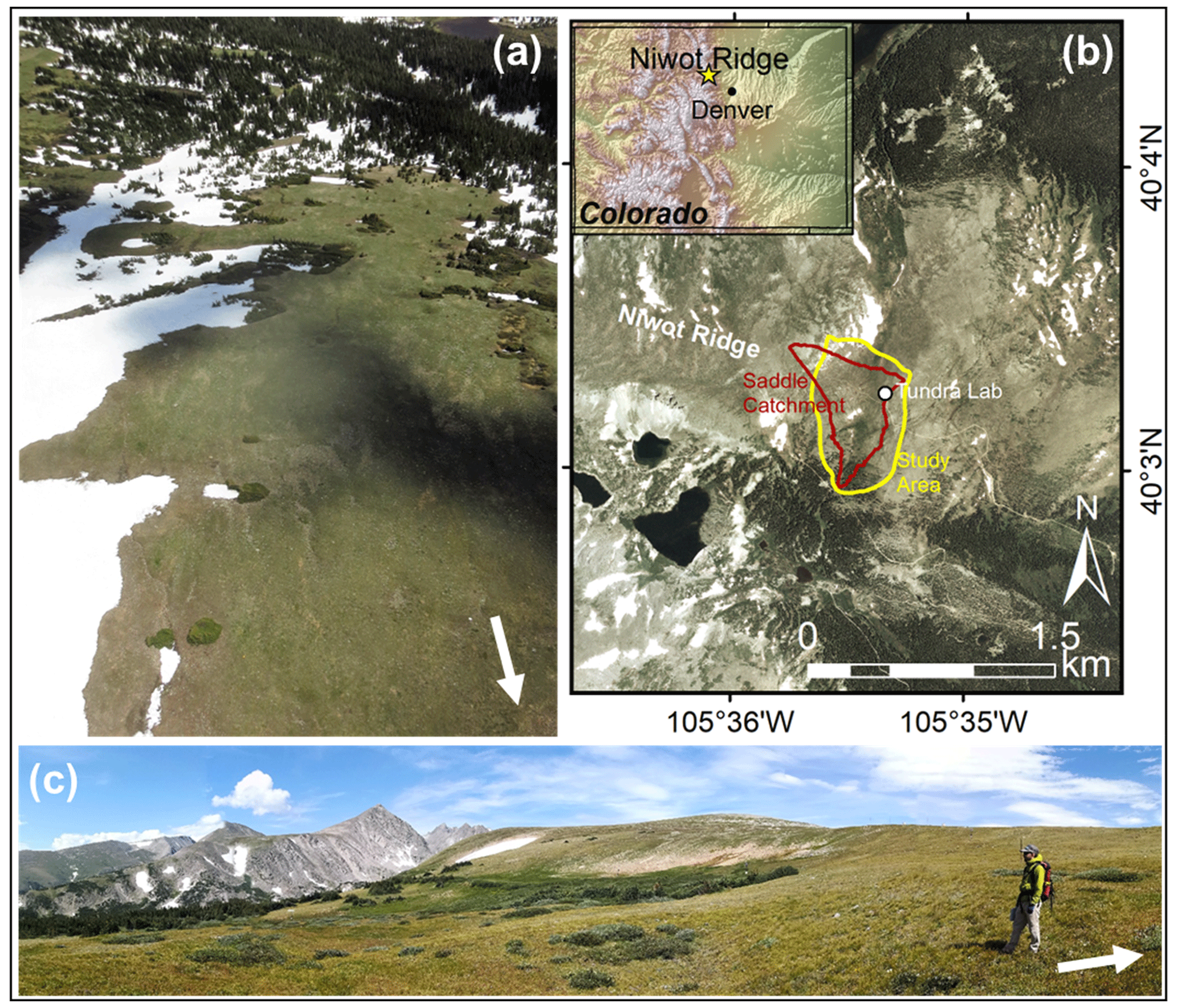
Figure 1Study site at Niwot Ridge (white arrows on photos indicate north). (a) Oblique aerial image of the study site looking downslope (south) from the northern edge, (b) study site location and relevant boundaries, and (c) terrestrial view of the study site from the eastern edge of the study site looking west. Base imagery in panel (b) sourced from the public-access USA National Agricultural Imagery Program (NAIP) 2005.
The NWT LTER is located in the headwaters of the Boulder Creek watershed (Fig. 1), comprises a range of altitudinal environments and includes a number of different focussed study sites within it (Bjarke et al., 2021). Niwot Ridge is one of the most extensively studied alpine systems in the world and was a UNESCO Biosphere Reserve from 1979 to 2017, in addition to currently being a United States Forest Service (USFS) experimental ecology reserve and a National Ecological Observatory Network (NEON) study site. Here we focus on the upper reaches of the NWT LTER in the “saddle catchment” (40∘03′09.42′′ N, 105∘35′29.62′′ W), which has an elevation range of ∼3420–3620 m a.s.l. The saddle catchment is a roughly 40 ha alpine sub-catchment of Boulder Creek. The lower reaches (3420–3450 m a.s.l.) are densely forested, primarily with Limber Pine (Pinus flexilis) and Lodgepole Pine (Pinus contorta). This gives way to Engelmann Spruce (Picea engelmannii) and Subalpine Fir (Abies lasiocarpa) at higher elevation; here, krummholz are deformed by the strong winds and function as points of localised snow accumulation on the leeward side. Alpine tundra extends above this treeline-transition zone and includes a variety of low shrubs, cushion plants, grasses, sedges, mosses and lichens (Walker et al., 2001). This tundra zone can be separated into five broad communities: dry meadow, moist meadow, wet meadow, rocky fellfields and snow bed (May and Webber, 1982; Walker et al., 2001). The saddle catchment has become a recent focus of the NWT LTER's research activities, coinciding with the installation of a dense network of soil moisture/temperature and precipitation sensors in 2017 and the establishment of long-term snow manipulation studies in 2018 (Bjarke et al., 2021). These activities complement ongoing observations of plant community composition at the plot level and meteorologic data collection that have been made at the study site for the past decades. The saddle catchment lies within a NEON site (NIWO) established in 2015. NEON conducts annual airborne surveys (lidar and multi-spectral) of the site and maintains a network of meteorological, ecological and hydrological measurements and instrumentation nearby.
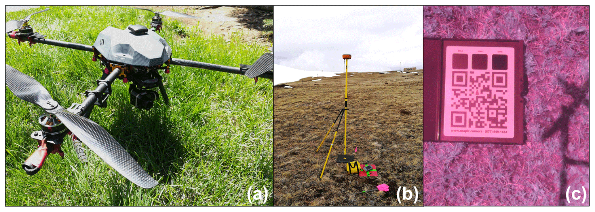
Figure 2Quadcopter UAS fitted with a thermal camera (a), installation and survey of GCPs (b), and a RNIR image of the surface reflectance calibration plate (c).
3.1 UAS platforms
We used two different multi-rotor UAS platforms: a hexacopter and a quadcopter (Fig. 2a). The multi-rotor platforms were custom-designed for operation in high-elevation mountain environments (4000–6000 m a.s.l.) (Wigmore and Mark, 2017; Wigmore et al., 2019). For this study we retuned the platforms to operate at 3500 m a.s.l. and to handle higher winds (∼10–22 m s−1), which requires faster speeds and motor-response times. Both platforms are constructed of carbon fibre to reduce weight and improve rigidity. The total weights of the systems excluding sensor payloads are 2.8 kg (hexacopter) and 2.4 kg (quadcopter); at the study-site elevation they are capable of around 15–20 min of flight (depending on wind speed) using a 4S 10 000 mAh lithium-polymer battery. They are equipped with the Pixhawk V1 flight controller and are capable of fully autonomous flight, including waypoint navigation and survey grids. The UAS can be manually controlled with a 2.4 GHz remote-control link; an RFD900+ 915 MHz telemetry downlink provides direct communication with the ground-control station, from where survey progress and flight information (ground speed, altitude, attitude, etc.) can be observed. Surveys are planned and managed through the Ardupilot Mission Planner ground-control system running on a Windows-based field tablet.
The platforms were fitted with visible red/green/blue (RBG) (Canon S110), red/near-infrared (RNIR) (MAPIR Survey 2) and thermal-infrared (TIR) (FLIR Vue Pro R 320) cameras, providing a total of six spectral bands (dual red bands). The RNIR camera has a measured band-wavelength interval from ∼630–690 nm (peak at 660 nm) and ∼810–900 nm (peak at 850 nm), while for the RGB camera, the exact band wavelengths are unknown. For both the RGB and RNIR cameras, settings (shutter speed, ISO, f-stop, etc.) were kept constant for each survey to maintain a consistent camera response to surface reflectance. The RGB and RNIR cameras can be flown simultaneously (as they have a similar field of view) and were mounted on a vibration-reducing plate (but no gimbal). The TIR camera was flown separately as it requires a three-axis gimbal for image stabilisation and more closely spaced flight lines due to its much narrower field of view. All image capture is triggered by camera intervalometers (i.e. no position triggering by a flight controller, which minimises potential points of failure). The RNIR and TIR cameras have this intervalometer feature built in. For the Canon S110, we installed the Canon hack development kit (CHDK) and loaded the KAP_UAV.lua V3.8 script (CHDK, 2016), which allows automated control of numerous camera functions. The TIR camera is connected to the autopilot and geotags images with position and orientation information at the time of image capture, and RGB and RNIR images can be geotagged after the fact by time-stamp matching (but for this study were not).
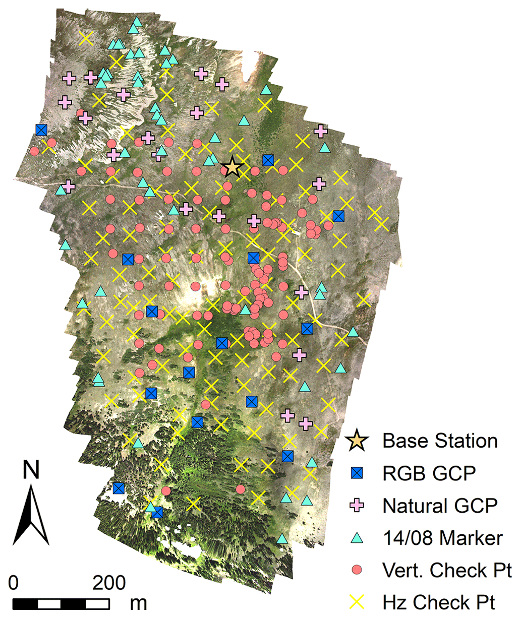
Figure 3Location of the local base station, all GCPs, and check points used in SfM processing and error assessment.
3.2 Ground control
In late May 2017 we permanently installed 15 visible ground-control points (GCPs) in snow-free regions of the study area (Fig. 3). Targets were 30 cm sheets of fluorescent Coroplast plastic, with a duct-tape cross marking the centre (Fig. 2b). We also installed and surveyed nine thermal targets (Wigmore et al., 2019); however, unfortunately these were not clearly visible in the imagery and were therefore not used as GCPs. To minimise propagation of errors in the structure-from-motion (SfM) photogrammetric processing and limit model “doming” (James and Robson, 2014; Tonkin and Midgley, 2016), we ensured targets were installed at the survey perimeter and at the topographic high and low points of the survey area. However, this was constrained by snow cover, limiting the number of GCPs in the north-western region. To mitigate this, an additional 22 natural-feature GCPs (e.g. isolated flat boulders ∼50–100 cm in diameter) were progressively surveyed as the snow melted to provide better GCP distribution over these areas (Fig. 3). Furthermore, an additional 48 co-registration markers were identified in the 14 August orthomosaic; their position and elevation were extracted from the DSM, and these were then used as extra markers for the earlier surveys when visible (Fig. 3). Not all GCPs and co-registration markers were used for each date due to some being obscured by snow, not imaged by the survey, poor visibility, and high error estimates. Details of which GCPs and markers were used for each survey are provided in their respective processing reports. A further 100 positions (Fig. 3) were surveyed during the field season for other projects occurring at the site (Hermes et al., 2020) and are used as vertical check points for accuracy assessment of the 14 August DSM. These positions were not specifically surveyed for the purposes of error assessment and thus do not have an ideal spatial distribution and may lie in areas of fine-scale topographic heterogeneity (local high/low points). The nine thermal GCPs were also used as vertical check points.
All GCPs and vertical check points were surveyed with a dual-frequency L1/L2 Altus APS3 global navigation satellite system (GNSS) receiver using a stop–go post-processed kinematic (PPK) methodology (Fig. 2b). Each position was occupied for 3 min at a 1 Hz interval. Base station observations were collected from a permanent UNAVCO-operated base station (station code NWOT) (Larson, 2009) (Trimble NetR9 receiver with Trimble Zephyr Geodetic antenna) located near the tundra lab at NWT (max baseline >1.5 km) and five National Geodetic Survey (NGS) continuous-reference stations (CORSs) from the surrounding area (station codes STBT, TMGO, P041, EC01 and COFC); 1 Hz L1/L2 GPS/GLONASS observations were used for each station. Rover positions were post-processed against the base-station network using Topcon Magnet Tools to an accuracy threshold of 2 cm horizontal and 5 cm vertical, and the mean standard deviations of point solutions were <1 cm (horizontal and vertical) for ground-target GCPs and <2 cm (horizontal and vertical) for natural-feature GCPs.
Table 1List of all survey-flight dates and imagery collected. TIR imagery was not collected on 27 June and 5 July due to deteriorating weather conditions and early thunderstorms.

3.3 UAS survey flights
Seven survey flights over the saddle catchment were completed from 21 June to 14 August (Table 1). Due to high, gusty winds and unstable weather (afternoon thunderstorms), we were unable to fly the exact same extent for each survey date. Flying around the crest of the ridge was particularly difficult in high winds (>18 m s−1) due to unstable eddies and downdrafts. We were unable to capture thermal imagery on 27 June and 5 July due to rapidly deteriorating weather conditions and approaching thunderstorms. Flight lines and image-capture intervals (every 3 s RGB and RNIR, every 1 s TIR) were selected to produce a >85 % front lap and a >65 % side lap. For each date we captured ∼400 RGB and ∼400 RNIR frames and ∼3000 TIR frames, ∼20 000 frames in total, for around 200 GB of raw data. The UASs are capable of terrain following, either from Google Earth base data (typically SRTM) or from custom digital elevation models (DEMs). In this case we used a 1 m lidar DEM of the study site, which helps to maintain a consistent ground-sampling distance during the survey and minimises the possibility of DEM terrain errors impacting automated return to launch procedures when flying downhill from the launch site. An above-ground-level (AGL) flight altitude of 120 m was selected to maximise area coverage (and minimise flight time) and remain within the legal limits of our Certificate of Authorisation (COA no. 2015-WSA-75-COA). This resulted in a ground resolution of approximately 4 cm for RGB and RNIR photo frames. RGB images were stored as *.jpg. RNIR images were captured as raw 14-bit *.tif (to enable later reflectance calibration with sufficient radiometric resolution). Thermal data were collected at roughly 25 cm ground resolution in 14-bit raw *.tif format (as opposed to FLIR's proprietary RJPG), which makes the data easier to work with in the processing and analysis stages.
SfM workflow
All data were processed using the SfM workflow as implemented in Agisoft Photoscan Pro V1.4. This commercial software has been widely used within the academic community, and numerous resources discuss its workflow in more detail (Verhoeven, 2011; Wigmore and Mark, 2017, 2018; Agisoft, 2016). The core workflow used for this study is summarised below. Complete details for the processing settings for each date can be found in the respective processing reports.
-
Image tie-point generation, alignment and sparse point-cloud creation utilising band 1 of all images (RGB/RNIR/TIR) simultaneously. The key-point limit is set to 120 000, the tie-point limit to 30 000 and the alignment accuracy to the highest value.
-
Identification of surveyed GCPs and 14 August co-registration marker locations in each image they are visible. TIR images were not included in this step as RGB GCPs were not visible in the TIR imagery.
-
Optimisation of sparse cloud, i.e. forcing sparse cloud into real-world coordinates of the GCPs.
-
Thinning of sparse point cloud to remove outlier points based on parameters of reprojection error (<1), reconstruction uncertainty (<50) and projection accuracy (<10).
-
Optimisation and sparse-cloud thinning were done iteratively up to three times to bring error estimation under 1 pixel (3 cm pixel) and >0.01 m combined positional error.
-
Dense cloud generation based on RGB imagery only, with high-quality and aggressive point-cloud filtering settings.
-
Triangular irregular network (TIN) mesh generated from RGB dense cloud.
-
TIN mesh smoothed and orthomosaics produced for each imagery dataset at both 5 cm (RGB, RNIR) and 25 cm (RNIR and TIR) pixel sizes.
After SfM processing, the RNIR geotif values were converted to surface reflectance in the red and near-infrared bands using the MAPIR QGIS plugin in combination with images of the MAPIR surface reflectance calibration targets that were collected during the flight (Fig. 2c). The near-Lambertian calibration targets comprise three plates of varying reflectance: white (87 % reflectance), grey (51 % reflectance) and black (23 % reflectance), with known surface reflectance between 350 and 1100 nm. From these radiometrically calibrated red and near-infrared image bands, normalised difference vegetation index (NDVI) maps were calculated for each date. TIR imagery was converted to surface temperature (Ts) in degrees Celcius using the FLIR factory conversion factor in Eq. (1).
Thermal images were processed simultaneously with RGB/RNIR data for the respective survey date (workflow above). However, an additional step is included in the TIR data-processing workflow to mitigate image vignetting. Thermal images captured with low-cost uncooled microbolometers often suffer from image vignetting where temperatures measured at the edges of the frame are systematically lower than those closer to the image centre (Kelly et al., 2019). Built-in non-uniformity-correction (NUC) algorithms aim to mitigate these errors, but cooler measurements are often still returned from the image periphery. To mitigate this vignetting, we applied a manually delineated ellipsoid vignette mask to each of the thermal images. This mask excludes data from the image edges from the final thermal orthomosaic.
To assess the horizontal positional error of the RGB imagery, we identified 101 stable image features (large rocks) that were relatively evenly distributed across the 14 August 5 cm RGB orthomosaic. We then measured the horizontal offset between the 14 August image and each orthomosaic date for which the horizontal check points were visible. Some horizontal check points were not visible on the earlier dates due to snow cover. Offset statistics (relative to the 14 August position) for each date and the entire series were then calculated. Vertical DSM error was assessed by comparing the 14 August DSM against the 109 surveyed vertical check points (above).
5.1 Processing results
Results of the processing accuracy, alignment errors and GCP positioning accuracy are provided within the processing report .pdf files for each survey date. Roughly 20 000 individual images were collected and processed. The surveyed area ranged from 0.58 to 0.80 km2 with a maximum ground-sampling distance of 4.11 to 4.22 cm (RGB). Reprojection error ranged from 0.783 to 1.1 pixels. Point-cloud density for the 14 August survey was 146 pts m−2, which is sufficient for DSM resolutions as fine as ∼10 cm.
Table 2Summary of available datasets and filename extensions as provided on the EDI portal.
a Wigmore (2022c); b Wigmore (2022a); c Wigmore and Niwot Ridge LTER (2022b); d Wigmore and Niwot Ridge LTER (2021a); e Wigmore and Niwot Ridge LTER (2021b); f Wigmore and Niwot Ridge LTER (2022a).
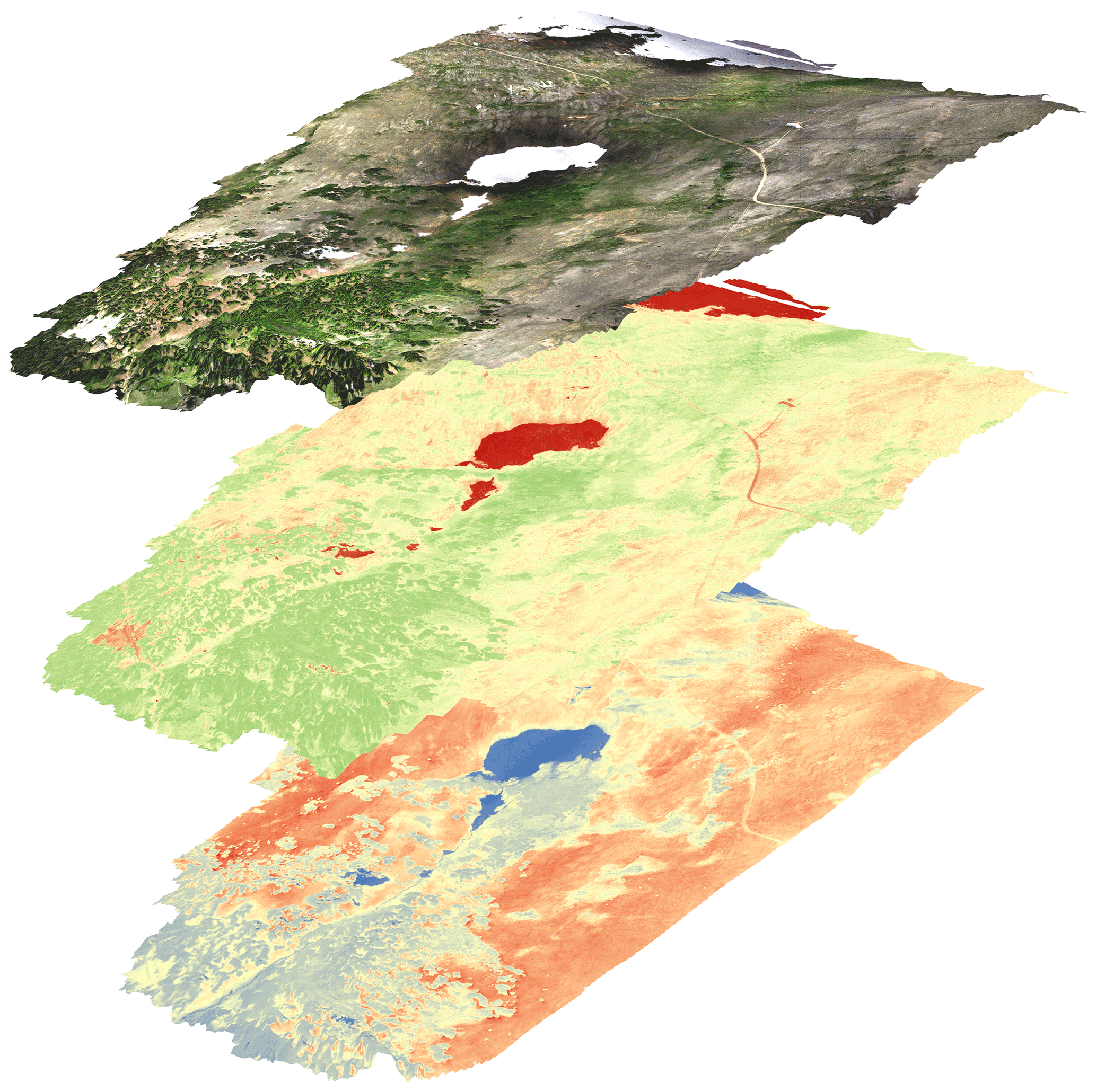
Figure 4Full data stack collected on 11 July 2017 showing RGB (top), NDVI (middle), and TIR (Ts) (bottom) draped over the 14 August 2017 DSM.
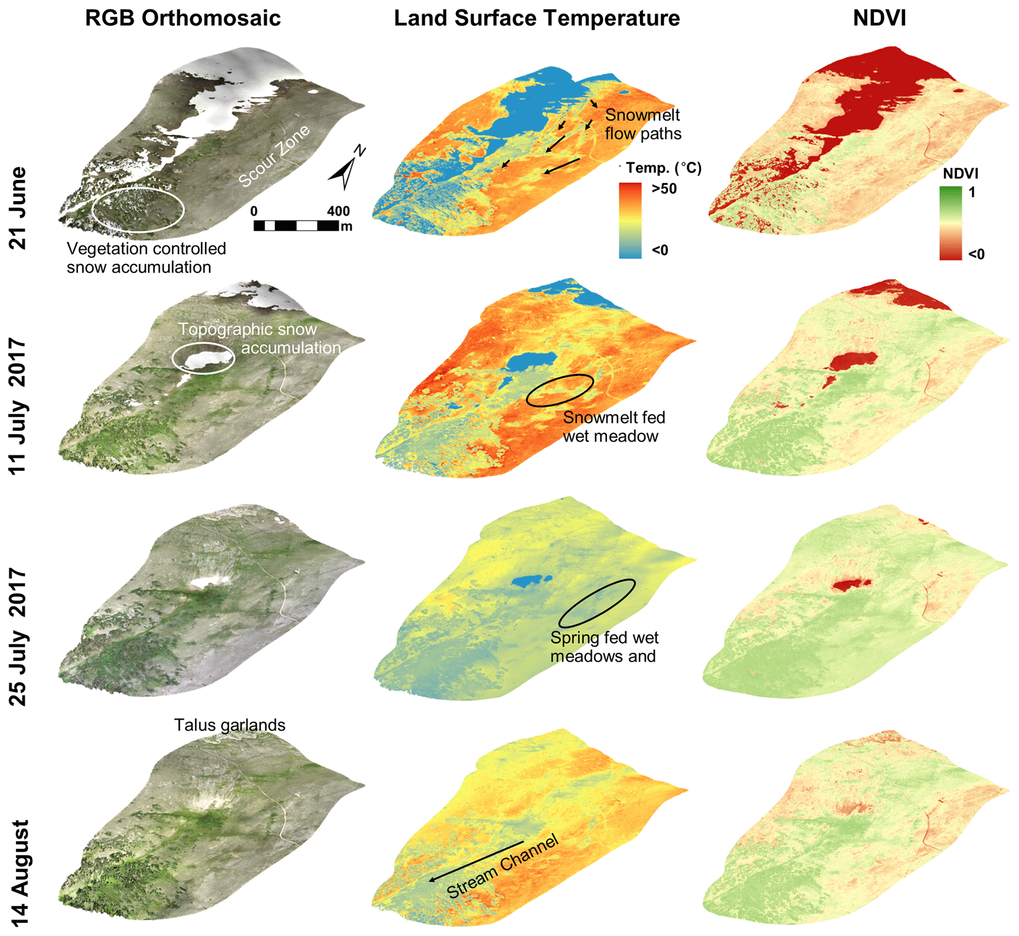
Figure 5Three-dimensional views of selected RGB orthomosaics (5 cm), Ts maps (from TIR) (25 cm), and NDVI (25 cm) draped over the 14 August 10 cm DSM.
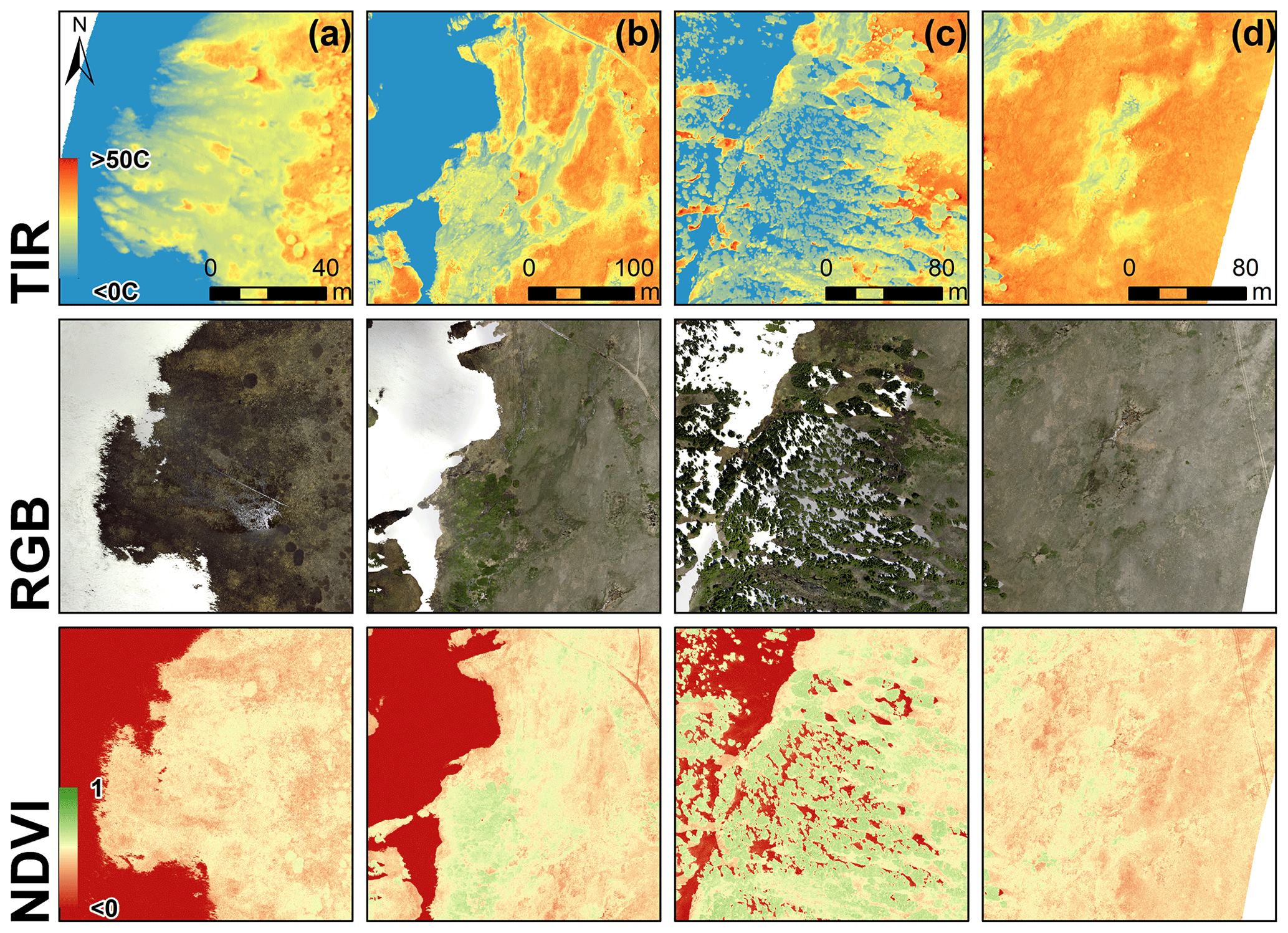
Figure 6Close-up of TIR (Ts) (top row) (25 cm), RGB (middle row) (5 cm), and NDVI (bottom row) (5 cm) image pairs for 21 June 2017. (a) Snowmelt pathways through wet meadow; (b) snowmelt feeding wet meadow; (c) snow accumulation in the forest zone; (d) surface ponds fed by sub-surface hydrologic pathways.
5.2 Multi-spectral and thermal mapping data overview
Figure 4 displays a full stack of data collected on 11 July 2017 and includes RGB imagery, NDVI (from the RNIR camera), and surface temperature from the TIR camera, draped over the 14 August DSM. Data available for each date are summarised in Table 2. Figure 5 displays RGB, TIR and NDVI orthomosaics draped over the 14 August DSM for a select number of the survey dates. Surface processes of snowmelt and vegetation green-up are clearly visible in the images. The high resolution of the RGB data facilitates the delineation of different vegetation types and land cover classes. Changes in snow extent can be readily delineated and quantified. The co-temporal TIR imagery provides an insight into the snowmelt-fed surface and sub-surface hydrologic pathways that are present, which are visible as cold streams across the landscape. The radiometrically calibrated NDVI image series facilitates quantitative assessment of changes in vegetation health and productivity (NDVI pixel value) over the survey period. Figure 6 is a close-up view of different areas on the 21 June survey date showing TIR, RGB and NDVI orthomosaics. Clearly visible in the thermal imagery are linear features of colder surface temperatures: these are suggestive of overland flow associated with snowmelt from the snow drifts (Fig. 6a and b). Wind redistribution and deposition of snow is evident, with areas of snow accumulation visible on the leeward side of trees and visible on the leeward side of trees and in topographic depressions (Fig. 6c). Meanwhile, the eastern side of the catchment is snow free for all survey dates (Fig. 5). Site visits during the winter-accumulation months indicate that this eastern edge is a wind-scour zone and is regularly cleared of snow during the winter months. Using the TIR imagery, we can also hypothesise the existence of sub-surface hydrologic pathways. For example, the wet meadows and surface ponds in Fig. 6d are not visibly connected to surface meltwater channels; however, they retain water late in the summer and maintain cold temperatures throughout the summer, suggesting these systems are potentially fed by groundwater springs (Wigmore et al., 2019; Lee et al., 2016; Hoffmann et al., 2014; Eschbach et al., 2017).
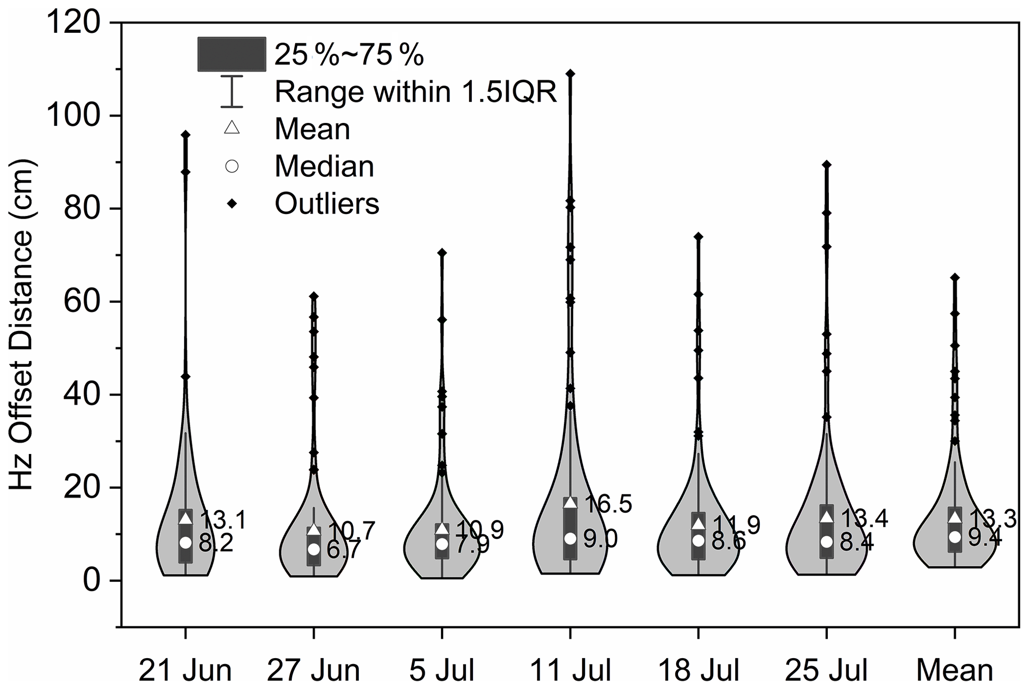
Figure 7Horizontal (Hz) offset at check-point locations for each survey date's RGB 5 cm orthomosaic relative to the 14 August position. The mean horizontal offset is shown in the right violin plot. Mean and median values labelled accordingly. The curve represents the kernel-smoothed frequency distribution of offsets.
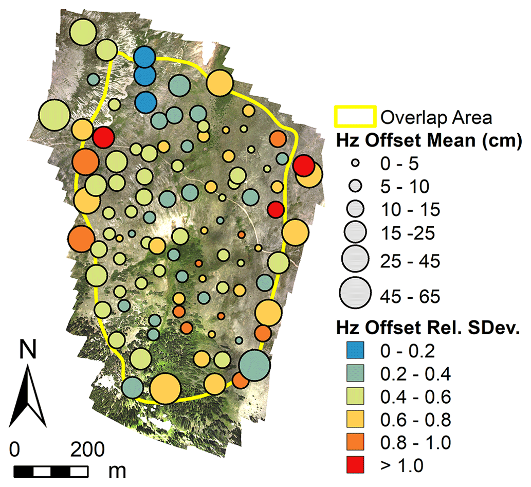
Figure 8Spatial distribution of horizontal (Hz) offset errors compared to the 14 August position.
5.3 Positional accuracy
The horizontal accuracy for each survey date relative to the 14 August survey is shown in Fig. 7 along with the combined (mean) offset for all the dates. The mean offset for the horizontal check points is 13.3 cm, with a median value of 9.4 cm and an interquartile range of 6.2 to 15.7 cm. Figure 8 shows the spatial distribution of these errors. Here, circle size indicates the magnitude of the mean horizontal offset, while circle colour indicates the relative standard deviation of the offset errors. Horizontal error is higher at the periphery of the survey area, where image overlap is lower and camera geometry is worse. Within the area overlapped by all the survey dates (yellow boundary line), the mean horizontal-offset error is mostly less than 15 cm, with a lower relative standard deviation. Therefore, limiting analysis to the area within the overlap boundary and working at pixel resolutions greater than 20 cm should minimise the impact of horizontal-offset (co-registration) errors on results.
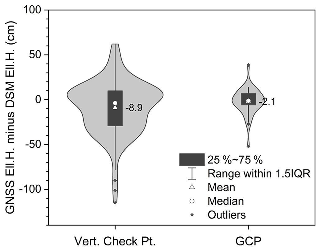
Figure 9Difference between GNSS ellipsoid height and 14 August DSM ellipsoid height for 109 check points and 37 GCPs. Negative values indicate that DSM elevation is greater than GNSS-surveyed elevation. Mean difference (cm) is shown in the plot. The curve represents the kernel-smoothed frequency distribution of vertical differences.
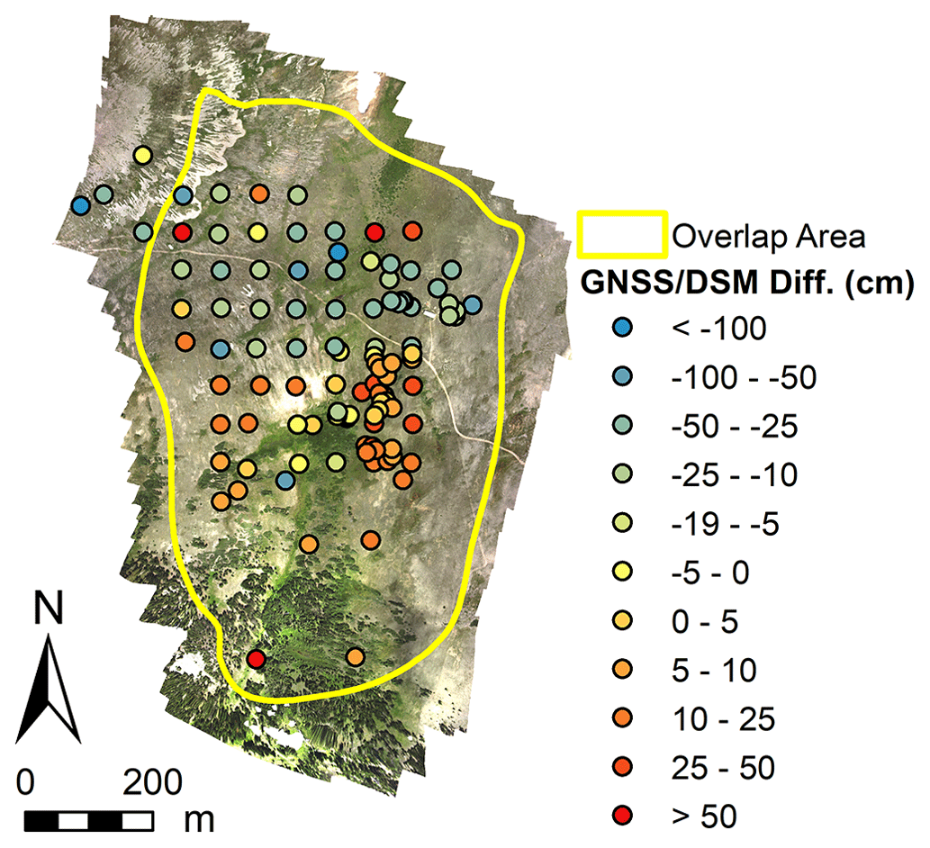
Figure 10Spatial distribution of vertical errors for the 14 August DSM (GNSS ellipsoid height at surveyed check points minus DSM ellipsoid height). Negative values indicate that DSM elevation is greater than GNSS-surveyed elevation.
Vertical accuracy for the 14 August DSM was assessed relative to GNSS-surveyed positions. Figure 9 displays the ellipsoid height difference between the 14 August 10 cm DSM surface and the 109 surveyed GNSS vertical check points as well as the 37 GCP locations (including targets and natural features). DSM elevation was subtracted from GNSS ground elevation, therefore negative values indicate that the DSM elevation is higher than the surveyed ground elevation. The mean GCP difference was −2.1 cm, with an interquartile range of −5.8 to 7.3 cm. As expected, this is very low, as the SfM model is forced to fit these GCP locations. For the vertical check points, the median difference is −8.9 cm, with an interquartile range of −29.0 to 9.9 cm. Data are visibly negatively skewed; i.e. DSM is higher than ground elevation. This is likely due to vegetation growth, as has been reported previously (Wigmore and Mark, 2018; Li et al., 2020). Figure 10 shows the spatial distribution of the vertical errors. Three notable outliers (1.5× interquartile range) are visible in the data (Fig. 9) with errors around cm: this is higher than expected. Inspection of Fig. 10 shows that one of the outlier values is located at the north-western edge of the survey area and is thus likely a result of doming in the DSM due to poor camera geometry (James and Robson, 2014). However, the other significant outliers are located around the middle of the survey area, where the survey geometry is more robust. It is possible that in this case the errors are associated with the vertical check-point data themselves as these positions were not collected specifically for this application and may not have been collected over stable and relatively uniform areas suitable for assessing the accuracy of the DSM (Wigmore and Mark, 2017).
6.1 Data availability
All data are made available through the LTER Data Portal of the Environmental Data Initiative (EDI) (Table 3) and are made available under the Creative Commons Attribution License, CC BY 4.0. Data are organised into six groups as follows: (1) 5 cm RGB orthomosaics (Wigmore, 2022c); (2) 5 and 25 cm RNIR orthomosaics (Wigmore, 2022a); (3) 5 cm multi-spectral orthomosaics (Wigmore and Niwot Ridge LTER, 2021a); (4) 25 cm TIR orthomosaics (Wigmore and Niwot Ridge LTER, 2022b); (5) NDVI datasets (Wigmore and Niwot Ridge LTER, 2021b); (6) elevation datasets (14 August 2017) (Wigmore and Niwot Ridge LTER, 2022a). Full-extent data include 5 cm RGB, 5 cm RNIR, 25 cm RNIR and 25 cm TIR (where available) at the maximum survey coverage. Data along the survey periphery are likely to suffer from increased positional errors due to the reduced number of images (lower overlap) and relatively poor camera geometry over these regions; these areas should therefore be clipped prior to analytical use. Clipped multi-spectral data include 5 cm RGB and RNIR imagery stacked in a single multi-band *.tif file that has been clipped to the maximum extent covered by all survey dates, including a buffer to mitigate low-quality data at the periphery. Spectral bands are as follows: B1 Blue (uncalibrated), B2 Green (uncalibrated), B3 Red (uncalibrated), B4 Red (calibrated surface reflectance centred at 660 nm) and B5 NIR (calibrated surface reflectance centred at 850 nm); 25 cm TIR orthomosaics are all provided as a clipped version in which data have been clipped to the same boundary as above (though coverage may be lower for these TIR surveys) and are provided as a 32-bit floating-point raster with units of degrees Celsius. NDVI data compile NDVI for each date into a single multi-band stack where each band corresponds to a survey date in series, i.e. B1 NDVI 21 June, B2 NDVI 28 June, B3 NDVI 5 July, etc. Basic analytical layers derived from this stack are also provided, including the maximum/peak NDVI value from the NDVI stack and the survey date on which this was measured, stored as a day-of-year integer value. Elevation data include the 14 August DSM (in *.tif) and an unclassified RGB-coloured point cloud (in *.laz). The DSM is derived from the unclassified point cloud and can thus be considered representative of vegetation canopy surface elevation. For much of the study site vegetation is very short (<5 cm) or absent (bare ground), and for these areas the DSM is equivalent to ground elevation; this is not the case for forested areas in the southern section of the study area. For all raster datasets individual metadata are included as an *.xml file in the ESRI ArcMap format and point-cloud data are accompanied by a *.txt readme metadata file. Unclipped RGB 5 cm datasets are also accompanied by the SfM processing report created by Agisoft Photoscan Pro software, which documents the processing parameters used and the GCP error for each survey date (Wigmore, 2022c).
6.2 Data caveats and considerations
Data are provided at both 5 cm (RGB, RNIR) and 25 cm (RNIR, TIR) spatial resolutions on aligned raster grids. Due to the lack of gimbal stabilisation (RGB and RNIR) and high winds at the site, the 5 cm imagery suffers from localised areas of image blur. Additionally, at this highest resolution the impact of potential offsets between the RGB and RNIR bands and between dates is increased. Therefore, for analytical purposes it is recommended that the data be aggregated to a coarser (>10 cm) spatial resolution. RGB data are uncalibrated and are likely unsuitable for analytical uses outside of mapping/classification. RNIR data are calibrated to surface reflectance for each date and thus can be used to calculate reliable NDVI values that are stable across the data series. Thermal data have not been calibrated with more accurate near-surface Ts measurements and thus can be assumed to be accurate to, at best, ±5 % or 5 ∘C per the manufacturer's (FLIR) documentation. Relative Ts differences are much higher resolution, with 0.04 ∘C pixel sensitivity recorded by the sensor. Thermal vignetting has been minimised through the masking process (above). Trends in the thermal data can originate from both cooling/warming of the scene during the survey window (∼1 h) and from warming-up of the thermal sensor. The latter was minimised by allowing the camera to warm up before image capture; however, the former is not addressed. Consequently, some north–south striping in the thermal mosaics is visible for some dates (e.g. 21 July 2017): this is a result of brief temporal gaps in flying while changing batteries. This is a common trade-off with small-format thermal imaging over large areas. Because of the lack of reliability in absolute Ts recovery for these datasets, it is recommended that users of the Ts data rely on them primarily for mapping thermal anomalies and relative differences, as opposed to deriving insight from absolute Ts values. File-naming conventions, spatial resolution and spectral bands are summarised in Table 2.
The complex topography and high degree of spatiotemporal variation present in mountain environments make them an ideal environment for the application of high-resolution UAS-based remote-sensing campaigns. Our mapping campaign leveraged both the high-spatial-resolution (centimetre) and high-temporal-resolution (weekly surveys) benefits of UAS while also capturing quantitative multi-spectral imagery over a relatively large area. There were a number of challenges to completing such a demanding survey protocol in a relatively hard-to-reach mountainous environment. These challenges can be summarised as technical and environmental challenges.
7.1 Technical challenges
Conversion of TIR to Ts for data collected from small microbolometer-type thermal sensors is a significant technical challenge. These sensors are prone to vignetting (Kelly et al., 2019) and warm up rapidly, which can bias measurements over time (Dugdale et al., 2019). Uniform emissivity corrections do not account for variations in land cover (and thus emissivity) within the scene (Aubry-Wake et al., 2015), and despite the relatively short distance to the target (∼120 m a.g.l.), there are often sufficient atmospheric effects to introduce measurement errors (FLIR, 2018; Torres-Rua, 2017). Furthermore, as the final image is a mosaic created from images collected over a ∼1 h window, warming or cooling of the scene can result in thermal trends within the orthomosaics. A number of solutions have been suggested to remedy these issues. Orthomosaics are frequently calibrated to higher-accuracy in-scene Ts measurements collected with non-contact infrared radiometers, temperature loggers and higher-quality thermal cameras (Kraaijenbrink et al., 2018; Torres-Rua, 2017; Wigmore et al., 2019). However, this bias correction does not account for changes in the scene temperature during the survey or drift errors induced by changes in the temperature of the camera. Individual frames can be calibrated prior to mosaicking, e.g. by correction to widespread surface features with stable Ts (e.g. melting snow at 0 ∘C) (Pestana et al., 2019); however, this is difficult to implement for large image collections, especially if the thermally stable feature is not visible in all image frames. Orthomosaics and/or individual images can also be classified by land cover type, with different emissivity values applied as appropriate (Aubry-Wake et al., 2015). Perhaps the most viable solution lies in technical innovations, for example the development of lightweight heated external shutters, which may increase measurement accuracy by as much as 70 % (TeAx, 2019). For this study we were less concerned with the accurate measurement of absolute Ts and more interested in mapping thermal anomalies and relative differences, for which microbolometer sensors are perfectly capable (Wigmore et al., 2019; Harvey et al., 2016; Dugdale et al., 2019; Poirier et al., 2013). However, where accurate measurements of Ts are required, these issues should be carefully considered and addressed in the planning stages.
For the collection of reliable time-series NDVI maps, RNIR raw-image digital numbers must be converted to surface reflectance. This calibration requires the imaging of known reflectance targets at the same time as the UAS survey and/or the collection of incident sunlight (scene illumination) through a secondary instrument (e.g. Parrot Sequoia and Micasense Red Edge multi-spectral cameras). For direct comparison of surface reflectance, the latter method is preferable as each image can be corrected individually (prior to ortho-mosaicking), thus accounting for temporary variations in illumination (e.g. passing clouds) during the survey-flight period. However, when comparing ratio indices, such as the NDVI, changing illumination is less of an issue, and therefore surface reflectance calibration based on reflectance targets is a suitable method (Hunt and Daughtry, 2018). It is important, however, that all camera settings, such as ISO, exposure length and aperture, remain constant during the survey, that sufficient radiometric depth is available (i.e. shooting in 12- or 16-bit RAW format, as opposed to 8-bit *.jpg) and that camera settings do not allow any part of the scenes' pixel values to saturate at the high or low end (overexpose or underexpose). Overexposure is of particular concern for snow-covered areas, where reflectance is high (Bühler et al., 2016; vander Jagt et al., 2015).
7.2 Environmental challenges
Environmental challenges were primarily related to site-specific atmospheric conditions that are typical of mountainous environments, specifically wind and altitude. Wind speeds at ground level were often in excess of 10 m s−1, with regular gusts at a flight altitude (120 m) of over 20 m s−1, which is at the upper limit of what many small UASs are designed to handle. A launch elevation of 3500 m a.s.l. is also sufficiently high to significantly reduce flight time due to lower air density. To deal with these two issues, we overhauled our existing UAS platforms, which were designed for higher elevations (>4500 m a.s.l.) but lower wind speeds in Peru's Cordillera Blanca (Wigmore et al., 2019; Wigmore and Mark, 2017). Our system was able to operate reliably in wind gusts of up to ∼22–24 m s−1. Live observations from the ground-station telemetry stream and flight logs showed periods of wind-induced pitch-and-roll compensation of up to 45∘ (the programmed limit). Designing UASs that are both robust and powerful enough to handle these forces is critical for reliable and repeatable mountain operations in sub-optimal conditions. The relatively lower elevation (3500 m a.s.l. as opposed to >4500 m a.s.l. in Peru) allowed us to add strength (and consequently weight) to the system. In this context, we used thicker-gauge carbon-fibre tubes and aluminium (as opposed to plastic) joint connectors, motor mounts, etc. while also seeing a ∼25–30 % increase in flight time, which increased from ∼14 min to ∼18 min on a 4S 10 000 mAh LiPO battery. Flight time is the critical limit on the maximum surveyable area. Multi-rotor systems are particularly limited in this respect (compared to fixed-wing platforms); however, multi-rotor systems are generally better at handling wind gusts. Long-flight-time multi-rotor systems are increasingly available; however, these are usually either very lightweight and thus weaker or are powered by high-efficiency (low-kilovolt, large-propeller) power systems which have slower response times and often lower maximum flight speeds, which limits their ability to deal with strong winds. Furthermore, these high-efficiency systems are usually larger and heavier, which limits their ability to be easily transported into the back country.
We presented the data-acquisition and data-processing methodology for a unique high-spatiotemporal-resolution series of UAS-derived datasets that includes centimetre-scale resolution RGB, RNIR and TIR imagery over a ∼40 ha study area in the Colorado Rockies collected approximately weekly over a summer-snowmelt season. These data are spatially coincident with the recently heavily instrumented NWT LTER saddle catchment. Almost 20 000 individual image frames were collected. These were processed using a SfM photogrammetric workflow and tied to absolute coordinates with a network of GNSS-surveyed GCPs. Horizontal co-registration errors were assessed by comparing the offset from the final (snow-free) survey and had a mean error of less than 20 cm for all the dates. The mean vertical accuracy of the DSM was 8.9 cm higher than the GNSS-surveyed position. Series of 5 cm (RGB, RNIR) and 25 cm (RNIR, TIR) orthomosaics are provided for each date along with a stack of 25 cm NDVI orthomosaics and NDVI summary data (peak NDVI and peak NDVI day of year). Elevation data for the snow-free (14 August 2017) survey include a DSM and high-density point cloud. Together these datasets provide a unique snapshot of summer snowpack, snowmelt, surface temperature and vegetation growth in a high alpine environment and facilitate the mapping and quantification of environmental variables and ecohydrologic processes at unprecedented spatial resolution. Potential applications for these data are many but include mapping of surface and sub-surface hydrologic connectivity, tracking vegetation productivity and seasonal green-up, mapping ecosystem zonation and quantifying distribution and changes in snow cover, snow depth and snowmelt. These data are made publicly available to facilitate broader use by the research community. These datasets leverage both the high spatial and temporal resolutions of UAS data capture while also collecting imagery across multiple spectral bands. As such these data may facilitate advances in our understanding of spatially and temporally dynamic ecohydrologic process and connectivity within alpine environments.
The video Drones over Niwot, (https://www.youtube.com/watch?v=5FxboPSCbW4&t=2s; Wigmore, 2022b) provides a brief summary of the project, output data, and potential applications; accompanied by dynamic geovisuals.
Both authors planned the objectives of the study. OW collected, processed and prepared all the datasets and prepared the draft manuscript. Both authors contributed to the revision and editing of the final manuscript.
The contact author has declared that neither of the authors has any competing interests.
Publisher's note: Copernicus Publications remains neutral with regard to jurisdictional claims in published maps and institutional affiliations.
We would like to thank members of the INSTAAR Mountain Hydrology Group for assistance with field data collection (GNSS survey) and UAS operations. We would also like to thank members of the Niwot Ridge LTER programme and the Mountain Research Station for logistical support and assistance. We would also like to thank the editor (James Thornton) and two reviewers (Marc Adams and Paul Schattan) for their constructive reviews and suggestions for improvement of the manuscript.
Oliver Wigmore was supported in part through funding from the University of Colorado 2016 Innovative Seed Grant (awarded to Noah P. Molotch), the University of Colorado Earth Lab Grand Challenge and the Niwot Ridge LTER programme (NSF DEB, grant no. 1637686). Additional support in the form of a GNSS equipment loan for the GNSS rover was provided by UNAVCO with support from the National Science Foundation (NSF) and the National Aeronautics and Space Administration (NASA) under an NSF Cooperative Agreement (grant no. EAR-0735156). Logistical support for this research was provided by the Niwot Ridge LTER programme (NSF DEB, grant no. 1637686).
This paper was edited by James Thornton and reviewed by Marc Adams and Paul Schattan.
Agisoft: Agisoft PhotoScan User Manual Standard Edition, Version 1.2, St. Petersburg: Agisoft LLC, 2016.
Aubry-Wake, C., Baraer, M., McKenzie, J. M., Mark, B. G., Wigmore, O., Hellström, R. Å., Lautz, L., and Somers, L.: Measuring glacier surface temperatures with ground-based thermal infrared imaging, Geophys. Res. Lett., 42, 8489–8497, https://doi.org/10.1002/2015GL065321, 2015.
Beniston, M.: Mountain weather and climate: a general overview and a focus on climatic change in the Alps, Hydrobiologia, 562, 3–16, https://doi.org/10.1007/s10750-005-1802-0, 2006.
Bjarke, N. R., Livneh, B., Elmendorf, S. C., Molotch, N. P., Hinckley, E.-L. S., Emery, N. C., Johnson, P. T. J., and Suding, K. N.: Catchment-scale observations at the Niwot Ridge Long-Term Ecological Research site, Hydrol. Process., 35, e14320, https://doi.org/10.1002/HYP.14320, 2021.
Bueno de Mesquita, C. P., Tillmann, L. S., Bernard, C. D., Rosemond, K. C., Molotch, N. P., and Suding, K. N.: Topographic heterogeneity explains patterns of vegetation response to climate change (1972–2008) across a mountain landscape, Niwot Ridge, Colorado, Arct. Antarct. Alp. Res., 50, e1504492, https://doi.org/10.1080/15230430.2018.1504492, 2018.
Bühler, Y., Adams, M. S., Bösch, R., and Stoffel, A.: Mapping snow depth in alpine terrain with unmanned aerial systems (UASs): potential and limitations, The Cryosphere, 10, 1075–1088, https://doi.org/10.5194/tc-10-1075-2016, 2016.
CHDK: KAP UAV Exposure Control Script, https://chdk.wikia.com/wiki/KAP_UAV_Exposure_ Control_Script (last access: 14 April 2023), 2016.
Christensen, L., Tague, C., and Baron, J. S.: Spatial patterns of transpiration response to climate variability in a snow-dominated mountain ecosystem, Hydrol. Process., 22, 3576–3588, 2008.
Colomina, I. and Molina, P.: Unmanned aerial systems for photogrammetry and remote sensing: A review, ISPRS J. Photogramm. Remote, 92, 79–97, https://doi.org/10.1016/j.isprsjprs.2014.02.013, 2014.
Dugdale, S. J., Kelleher, C. A., Malcolm, I. A., Caldwell, S., and Hannah, D. M.: Assessing the potential of drone-based thermal infrared imagery for quantifying river temperature heterogeneity, Hydrol. Process., 33, 1152–1163, https://doi.org/10.1002/hyp.13395, 2019.
Erickson, T. A., Williams, M. W., and Winstral, A.: Persistence of topographic controls on the spatial distribution of snow in rugged mountain terrain, Colorado, United States, Water Resour. Res., 41, 1–17, https://doi.org/10.1029/2003WR002973, 2005.
Eschbach, D., Piasny, G., Schmitt, L., Pfister, L., Grussenmeyer, P., Koehl, M., Skupinski, G., and Serradj, A.: Thermal-infrared remote sensing of surface water-groundwater exchanges in a restored anastomosing channel (Upper Rhine River, France), Hydrol. Process., 31, 1113–1124, https://doi.org/10.1002/hyp.11100, 2017.
Fagre, D. B., Peterson, D. L., and Hessl, A. E.: Taking the pulse of mountains: Ecosystem responses to climatic variability, in: Climatic Change, vol. 59, Springer, 263–282, https://doi.org/10.1023/A:1024427803359, 2003.
FLIR: Tech Note: Radiometric Temperature Measurements Surface Characteristics and Atmospheric Compensation, https://www.flir.com/globalassets/guidebooks/suas-radiometric-tech-note-en.pdf (last access: 14 April 2023), 2018.
Fonstad, M. A., Dietrich, J. T., Courville, B. C., Jensen, J. L., and Carbonneau, P. E.: Topographic structure from motion: a new development in photogrammetric measurement, Earth Surf Process Landf, 38, 421–430, https://doi.org/10.1002/esp.3366, 2013.
Grünewald, T., Schirmer, M., Mott, R., and Lehning, M.: Spatial and temporal variability of snow depth and ablation rates in a small mountain catchment, Cryosphere, 4, 215–225, https://doi.org/10.5194/tc-4-215-2010, 2010.
Harvey, M. C., Rowland, J. V., and Luketina, K. M.: Drone with thermal infrared camera provides high resolution georeferenced imagery of the Waikite geothermal area, New Zealand, Journal of Volcanology and Geothermal Research, 325, 61–69, https://doi.org/10.1016/J.JVOLGEORES.2016.06.014, 2016.
Hermes, A. L., Wainwright, H. M., Wigmore, O. H., Falco, N., Molotch, N., and Hinckley, E.-L. S.: From patch to catchment: A statistical framework to identify and map soil moisture patterns across complex alpine terrain, Front. Water, 2, 48, https://doi.org/10.3389/FRWA.2020.578602, 2020.
Hoffmann, H., Müller, S., and Friborg, T.: Using an unmanned aerial vehicle (UAV) and a thermal infrared camera to estimate temperature differences on a lake surface, revealing incoming groundwater seepage, in: EGU General Assembly Conference Abstracts, 6234, https://doi.org/10.13140/RG.2.1.4596.1840, 2014.
Hunt, E. R. and Daughtry, C. S. T.: What good are unmanned aircraft systems for agricultural remote sensing and precision agriculture?, Int. J. Remote Sens., 39, 5345–5376, https://doi.org/10.1080/01431161.2017.1410300, 2018.
Ives, J. D., Messerli, B., and Spiess, E.: Mountains of the world: A global priority, in: Mountains of the World: A Global Priority, edited by: Messerli, B. and Ives, J. D., The Parthenon Publishing Group Inc., Pearl River, New York, 1, 1997.
James, M. R. and Robson, S.: Mitigating systematic error in topographic models derived from UAV and ground-based image networks, Earth Surf. Process. Landf., 39, 1413–1420, https://doi.org/10.1002/esp.3609, 2014.
Kelly, J., Kljun, N., Olsson, P.-O., Mihai, L., Liljeblad, B., Weslien, P., Klemedtsson, L., and Eklundh, L.: Challenges and Best Practices for Deriving Temperature Data from an Uncalibrated UAV Thermal Infrared Camera, Remote Sens.-Basel, 11, 567, https://doi.org/10.3390/rs11050567, 2019.
Kraaijenbrink, P., Shea, J. M., Litt, M., Steiner, J. F., Treichler, D., Koch, I., and Immerzeel, W. W.: Mapping surface temperatures on a debris-covered glacier with an unmanned aerial vehicle, Front. Earth Sci.-Lausanne, 6, https://doi.org/10.3389/feart.2018.00064, 2018.
Larson, K.: GPS Soil Moisture Network – NWOT-Niwot Ridge P.S., https://doi.org/10.7283/T5VQ30RT, 2009.
Lee, E., Yoon, H., Hyun, S. P., Burnett, W. C., Koh, D.-C., Ha, K., Kim, D., Kim, Y., and Kang, K.: Unmanned aerial vehicles (UAVs)-based thermal infrared (TIR) mapping, a novel approach to assess groundwater discharge into the coastal zone, Limnol. Oceanogr. Methods, 14, 725–735, https://doi.org/10.1002/lom3.10132, 2016.
Li, D., Wigmore, O., Durand, M. M. T., Vander-Jagt, B., Margulis, S. A. S. A., Molotch, N. P. N., and Bales, R. R. C.: Potential of balloon photogrammetry for spatially continuous snow depth measurements, IEEE Geosci. Remote Sens. Lett., 17, 1667–1671, https://doi.org/10.1109/LGRS.2019.2953481, 2020.
Litaor, M. I., Williams, M., and Seastedt, T. R.: Topographic controls on snow distribution, soil moisture, and species diversity of herbaceous alpine vegetation, Niwot Ridge, Colorado, J. Geophys. Res.-Biogeo., 113, 2008, https://doi.org/10.1029/2007JG000419, 2008.
May, D. E. and Webber, P. J.: Spatial and temporal variation of the vegetation and its productivity, Niwot Ridge, Colorado, 1982.
Pape, R., Wundram, D., and Löffler, J.: Modelling near-surface temperature conditions in high mountain environments: an appraisal, Clim. Res., 39, 99–109, https://doi.org/10.3354/cr00795, 2009.
Pestana, S., Chickadel, C. C., Harpold, A., Kostadinov, T. S., Pai, H., Tyler, S., Webster, C., and Lundquist, J. D.: Bias Correction of Airborne Thermal Infrared Observations Over Forests Using Melting Snow, Water Resour. Res., 55, 11331–11343, https://doi.org/10.1029/2019WR025699, 2019.
Poirier, N., Hautefeuille, F., and Calastrenc, C.: Low altitude thermal survey by means of an automated unmanned aerial vehicle for the detection of archaeological buried structures, Archaeol. Prospect, 20, 303–307, https://doi.org/10.1002/arp.1454, 2013.
TeAx: Extended Value: External Shutter for FLIR Vue Pro R – Increased temperature accuracy by up to 70 %, https://thermalcapture.com/extended-value-external-shutter-for-flir-vue-pro-r/, last access: 10 December 2019.
Tonkin, T. N. and Midgley, N. G.: Ground-control networks for image based surface reconstruction: An investigation of optimum survey designs using UAV derived imagery and structure-from-motion photogrammetry, Remote Sens.-Basel, 8, 16–19, https://doi.org/10.3390/rs8090786, 2016.
Torres-Rua, A.: Vicarious calibration of sUAS microbolometer temperature imagery for estimation of radiometric land surface temperature, Sensors, 17, 1499, https://doi.org/10.3390/s17071499, 2017.
Trujillo, E., Ramírez, J. A., and Elder, K. J.: Topographic, meteorologic, and canopy controls on the scaling characteristics of the spatial distribution of snow depth fields, Water Resour. Res., 43, W07409, https://doi.org/10.1029/2006WR005317, 2007.
Trujillo, E., Molotch, N. P., Goulden, M. L., Kelly, A. E., and Bales, R. C.: Elevation-dependent influence of snow accumulation on forest greening, Nat. Geosci., 5, 705–709, https://doi.org/10.1038/ngeo1571, 2012.
vander Jagt, B., Lucieer, A., Wallace, L., Turner, D., and Durand, M.: Snow Depth Retrieval with UAS Using Photogrammetric Techniques, Geosciences-Basel, 5, 264–285, https://doi.org/10.3390/geosciences5030264, 2015.
Verhoeven, G.: Taking computer vision aloft – archaeological three-dimensional reconstructions from aerial photographs with photoscan, Archaeol. Prospect., 18, 67–73, https://doi.org/10.1002/arp.399, 2011.
Vivoni, E. R., Rango, A., Anderson, C. A., Pierini, N. A., Schreiner-McGraw, A. P., Saripalli, S., and Laliberte, A. S.: Ecohydrology with unmanned aerial vehicles, Ecosphere, 5, art130, https://doi.org/10.1890/ES14-00217.1, 2014.
Walker, M. D., Walker, D. A., Theodose, T. A., and Webber, P. J.: The vegetation: hierarchical species-environment relationships, in: Alpine Ecosystem: Niwot Ridge, Colorado, edited by: Bowman, W. D. and Seastedt, T. R., Oxford University Press, Incorporated, 99–127, 2001.
Watts, A. C., Ambrosia, V. G., and Hinkley, E. A.: Unmanned aircraft systems in remote sensing and scientific research: Classification and considerations of use, Remote Sens.-Basel, 4, 1671–1692, https://doi.org/10.3390/rs4061671, 2012.
Wieder, W. R., Knowles, J. F., Blanken, P. D., Swenson, S. C., and Suding, K. N.: Ecosystem function in complex mountain terrain: Combining models and long-term observations to advance process-based understanding, J. Geophys. Res.-Biogeo., 122, 825–845, https://doi.org/10.1002/2016JG003704, 2017.
Wigmore, O.: Calibrated Red/Near Infrared orthomosaic imagery from UAV campaign at Niwot Ridge, 2017. ver 1., Environmental Data Initiative [data set], https://doi.org/10.6073/pasta/dadd5c2e4a65c781c2371643f7ff9dc4, 2022a.
Wigmore, O.: Drones over Niwot, YouTube [video], https://www.youtube.com/watch?v=5FxboPSCbW4&t=2s (last access: 10 April 2023), 2022b.
Wigmore, O.: Uncalibrated RGB orthomosaic imagery from UAV campaign at Niwot Ridge, 2017. ver 1., Environmental Data Initiative [data set], https://doi.org/10.6073/pasta/073a5a67ddba08ba3a24fe85c5154da7, 2022c.
Wigmore, O. and Mark, B.: Monitoring tropical debris-covered glacier dynamics from high-resolution unmanned aerial vehicle photogrammetry, Cordillera Blanca, Peru, The Cryosphere, 11, 2463–2480, https://doi.org/10.5194/tc-11-2463-2017, 2017.
Wigmore, O. and Mark, B.: High altitude kite mapping: evaluation of kite aerial photography (KAP) and structure from motion digital elevation models in the Peruvian Andes, Int. J. Remote Sens., 39, 4995–5015, https://doi.org/10.1080/01431161.2017.1387312, 2018.
Wigmore, O. and Niwot Ridge LTER: 5 cm multispectral imagery from UAV campaign at Niwot Ridge, 2017 ver 1., Environmental Data Initiative [data set], https://doi.org/10.6073/pasta/a4f57c82ad274aa2640e0a79649290ca, 2021a.
Wigmore, O. and Niwot Ridge LTER: 25 cm NDVI data from UAV campaign at Niwot Ridge Saddle Catchment, 2017 ver 1., Environmental Data Initiative [data set], https://doi.org/10.6073/pasta/444a7923deebc4b660436e76ffa3130c, 2021b.
Wigmore, O. and Niwot Ridge LTER: Photogrammetric Point Cloud and DSM from UAV campaign at Niwot Ridge, 2017. ver 2, Environmental Data Initiative [data set], https://doi.org/10.6073/pasta/1289b3b41a46284d2a1c42f1b08b3807, 2022a.
Wigmore, O. and Niwot Ridge LTER: Surface temperature mapped from thermal infrared survey from UAV campaign at Niwot Ridge, 2017. ver 2., Environmental Data Initiative [data set], https://doi.org/10.6073/pasta/70518d55a8d6ec95f04f2d8a0920b7b8, 2022b.
Wigmore, O., Mark, B., McKenzie, J., Baraer, M., and Lautz, L.: Sub-metre mapping of surface soil moisture in proglacial valleys of the tropical Andes using a multispectral unmanned aerial vehicle, Remote Sens. Environ., 222, 104–118, https://doi.org/10.1016/j.rse.2018.12.024, 2019.
Zhang, C. and Kovacs, J. M.: The application of small unmanned aerial systems for precision agriculture: A review, Precis. Agric., 13, 693–712, https://doi.org/10.1007/s11119-012-9274-5, 2012.