the Creative Commons Attribution 4.0 License.
the Creative Commons Attribution 4.0 License.
 | 12 Apr 2023
A global long-term, high-resolution satellite radar backscatter data record (1992–2022+): merging C-band ERS/ASCAT and Ku-band QSCAT
Shengli Tao
Jean-Pierre Wigneron
Sassan Saatchi
Philippe Ciais
Jérôme Chave
Thuy Le Toan
Pierre-Louis Frison
Xiaomei Hu
Lei Fan
Mengjia Wang
Jiangling Zhu
Xia Zhao
Xiaojun Li
Xiangzhuo Liu
Yanjun Su
Tianyu Hu
Qinghua Guo
Zhiheng Wang
Zhiyao Tang
Yi Y. Liu
Jingyun Fang
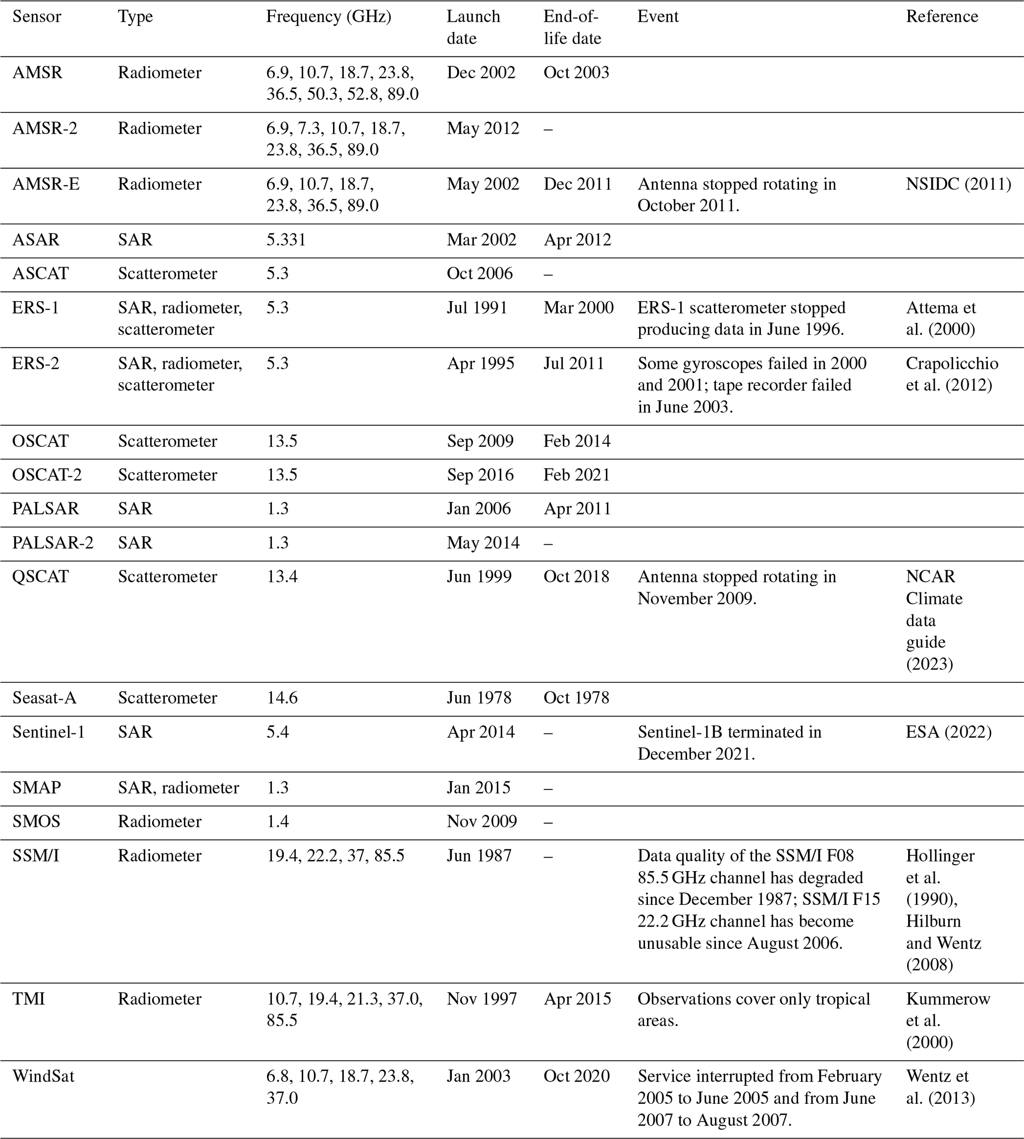
Satellite radar backscatter contains unique information on land surface moisture, vegetation features, and surface roughness and has thus been used in a range of Earth science disciplines. However, there is no single global radar data set that has a relatively long wavelength and a decades-long time span. We here provide the first long-term (since 1992), high-resolution (∼8.9 km instead of the commonly used ∼25 km resolution) monthly satellite radar backscatter data set over global land areas, called the long-term, high-resolution scatterometer (LHScat) data set, by fusing signals from the European Remote Sensing satellite (ERS; 1992–2001; C-band; 5.3 GHz), Quick Scatterometer (QSCAT, 1999–2009; Ku-band; 13.4 GHz), and the Advanced SCATterometer (ASCAT; since 2007; C-band; 5.255 GHz). The 6-year data gap between C-band ERS and ASCAT was filled by modelling a substitute C-band signal during 1999–2009 from Ku-band QSCAT signals and climatic information. To this end, we first rescaled the signals from different sensors, pixel by pixel. We then corrected the monthly signal differences between the C-band and the scaled Ku-band signals by modelling the signal differences from climatic variables (i.e. monthly precipitation, skin temperature, and snow depth) using decision tree regression.
The quality of the merged radar signal was assessed by computing the Pearson r, root mean square error (RMSE), and relative RMSE (rRMSE) between the C-band and the corrected Ku-band signals in the overlapping years (1999–2001 and 2007–2009). We obtained high Pearson r values and low RMSE values at both the regional (r≥0.92, RMSE ≤ 0.11 dB, and rRMSE ≤ 0.38) and pixel levels (median r across pixels ≥ 0.64, median RMSE ≤ 0.34 dB, and median rRMSE ≤ 0.88), suggesting high accuracy for the data-merging procedure. The merged radar signals were then validated against the European Space Agency (ESA) ERS-2 data, which provide observations for a subset of global pixels until 2011, even after the failure of on-board gyroscopes in 2001. We found highly concordant monthly dynamics between the merged radar signals and the ESA ERS-2 signals, with regional Pearson r values ranging from 0.79 to 0.98. These results showed that our merged radar data have a consistent C-band signal dynamic.
The LHScat data set (https://doi.org/10.6084/m9.figshare.20407857; Tao et al., 2023) is expected to advance our understanding of the long-term changes in, e.g., global vegetation and soil moisture with a high spatial resolution. The data set will be updated on a regular basis to include the latest images acquired by ASCAT and to include even higher spatial and temporal resolutions.
- Article
(9153 KB) - Full-text XML
-
Supplement
(3502 KB) - BibTeX
- EndNote


Microwave remote sensing uses electromagnetic radiation with a wavelength (λ) between 1 cm and 1 m as a measurement tool (Ulaby et al., 1982). Depending on the source of the energy from which the information is gathered, microwave remote sensing systems can be categorized into two groups, namely passive (radiometer) and active (radar). Passive systems collect the radiation naturally emitted by the observed surface, whereas active systems transmit a (radio) signal in the microwave bandwidth and record the signal backscattered by the target (Ulaby et al., 2014).
Due to the longer wavelength compared to visible and infrared radiation, microwaves exhibit the important property of penetrating objects, with the penetrating ability increasing with increasing wavelength. Microwaves at high frequencies (such as Ku-band; ∼13 GHz; cm) are sensitive to atmospheric conditions, but those at lower frequencies, such as C-band radio frequency (∼5 GHz; cm), depend less on cloud cover and heavy rain events, making this technique suitable for all weather conditions (Ulaby et al., 2014; Carabajal and Harding, 2006; Le Toan et al., 2011). As a result, long-wavelength microwave remote sensing has been widely used in Earth science studies for atmosphere, land, and ocean monitoring (Wentz, 1992; Wagner et al., 1999, 2007; Spreen et al., 2008; Shi et al., 2016; Steele-Dunne et al., 2017; Murfitt and Duguay, 2021).
However, there is no single multi-decadal microwave data set acquired at the C-band or longer wavelength that spans more than 2 decades (Table 1). This has limited the use of microwave data for trend analysis over extended time intervals. Several passive microwave systems are available, such as the Advanced Microwave Scanning Radiometer for EOS (Earth Observation Satellite; AMSR-E; 2002–2011), the Advanced Microwave Scanning Radiometer 2 (AMSR2; 2012–present), WindSat (2003–2012), Soil Moisture and Ocean Salinity (SMOS; 2010–now), and Soil Moisture Active Passive (SMAP; 2015–now), all of which provide data with a wavelength of ∼6 cm or longer (Spreen et al., 2008; Yao et al., 2021; Wigneron et al., 2017, 2021). However, merging them into a harmonized data set with a time span longer than 2 decades has been shown to be challenging, mainly because AMSR-E has no overlapping observations with AMSR2 (Du et al., 2017; Moesinger et al., 2020; Wang et al., 2021).
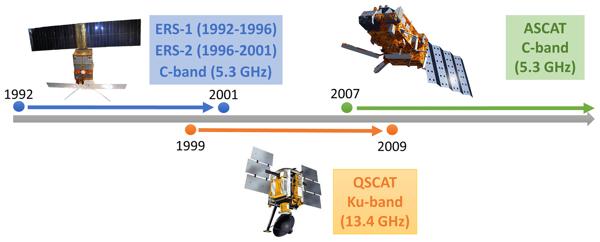
Figure 1Temporal coverages and radio frequencies of ERS-1/-2, QSCAT, and ASCAT. ERS-1/-2 and ASCAT have a C-band radio frequency (5.3 GHz), and QSCAT has a Ku-band frequency (13.4 GHz). QSCAT operated between 1999 and 2009 in full mode, overlapping with both ERS and ASCAT. Image courtesy of NASA and the European Space Agency (ESA).
Active microwave remote sensing, or radar, has the potential to overcome this limitation. A scatterometer is one type of radar known for its large footprint, global coverage, and high revisit rate. These properties make scatterometers interesting for the study of large-scale land surface dynamics (Ulaby et al., 2014). Spaceborne scatterometer sensors have been deployed since 1978 (NASA's Seasat-A; Ku-band; Table 1), but global coverage of scatterometer observation dates back to the European Remote Sensing satellite (ERS-1/-2) in the 1990s (C-band; from 1992 to 2001; Frison and Mougin, 1996; Prigent et al., 2001). Over the past 3 decades, multiple scatterometer missions have been launched with the aim of obtaining full and repeated global coverage (Ulaby et al., 2014), such as the Quick Scatterometer (QSCAT; Ku-band; from 1999 to 2009), the Oceansat-2 Scatterometer (OSCAT; Ku-band; since 2009), and the Advanced SCATterometer (ASCAT; C-band; since 2007). Among these sensors, both ERS-1/-2 and ASCAT operate at the C-band frequency but have a temporal gap of about 6 years (i.e. between 2001 and 2007). Filling this time gap would lead to the first global C-band scatterometer data set with continuous observations for the past 3 decades (since 1992). Moreover, this data set could, in principle, be further extended because ASCAT is still operational, and similar C-band radar missions have been secured for the future (such as the Sentinel radar series and the MetOp Second Generation satellite mission; Malenovský et al., 2012; Lin et al., 2016).
The present study aims at filling the 6-year gap of the C-band scatterometer data at the global scale (Fig. 1). As seen in Table 1, QSCAT is a good candidate for fulfilling this task because it operated between 1999 and 2009, thus overlapping with both ERS-2 (between 1999 and 2001) and ASCAT (between 2007 and 2009). Recent studies also demonstrated the feasibility of merging ERS-1/-2, QSCAT, and ASCAT (Bentamy et al., 2012; Tao et al., 2022; Frolking et al., 2022a, b). In theory, the Ku-band signal interacts more with smaller elements (such as raindrops, snow, and canopy leaves) than the C-band signal, due to the difference in wavelength (Saatchi et al., 2013). However, our previous work (Tao et al., 2022) has shown that the Ku-band QSCAT signal in tropical regions can be adjusted to the ERS-2 observations during 1999–2001 and to the ASCAT observations during 2007–2009 to obtain a simulated C-band signal (Tao et al., 2022). Here, we further extend our previous approach to the global scale through a better understanding of the signal mechanism and an improved technique for modelling the signal differences (i.e. decision tree regression). Image resolution has also been enhanced; while the native resolution of scatterometer images is often coarse (25 km or larger), the National Aeronautics and Space Administration (NASA) Scatterometer Climate Record Pathfinder (SCP; https://www.scp.byu.edu/, last access: 20 January 2023) project has improved the resolutions of ERS-1/-2, QSCAT, and ASCAT images using the scatterometer image reconstruction (SIR) with filtering (SIRF) algorithm, which combines multiple-orbit satellite passes (Long et al., 1993; Early and Long, 2001). Specifically, ERS-1/-2 images of 8.9 km resolution in the period of 1992–2001 and QSCAT (1999–2009) and ASCAT (2007–now) images of 4.45 km resolution have been made publicly available. To guarantee a long time span from 1992 onwards, we aggregated QSCAT and ASCAT images to 8.9 km to be consistent with the resolution of ERS-1/-2 images. We chose to produce a monthly radar data set in this study because daily scatterometer images do not provide full global coverage and also because the higher spatial resolution was achieved at the cost of reduced temporal resolution, with daily images only being available for polar regions (https://www.scp.byu.edu/docs/EnhancedFAQ.html, last access: 20 January 2023). Besides, the monthly time resolution has been frequently adopted by previous global-scale studies (Sun et al., 2018). The resulting merged radar data set, named long-term, high-resolution scatterometer (LHScat), is publicly available in netCDF format at https://doi.org/10.6084/m9.figshare.20407857 (Tao et al., 2023). LHScat will be constantly updated to include the latest images acquired by ASCAT and to include even higher spatial and temporal resolutions. Below, we provide a detailed illustration on the source data, methods, quality, and validation of the LHScat data set.
Table 1Basic information of commonly used satellite microwave sensors.
2.1 ERS-1/-2, QSCAT, and ASCAT data
Scatterometers were originally designed to measure wind speed and direction, particularly over oceans. However, their data have also been found to be useful for land applications such as soil moisture estimation, rainfall estimation, and forest monitoring. Here we analysed spaceborne scatterometer data from the ERS-1/-2, QSCAT, and ASCAT sensors (Fig. 1; Table 1). The backscatter of the radar signal, usually expressed in decibels (dB), is a function of the sensor parameters (frequency, polarization, look angle, and spatial resolution) and the dielectric and geometric properties of the scattering objects.
ERS-1, launched in 1991 by the European Space Agency (ESA), carries the first spaceborne C-band scatterometer with repeated and global geographical coverage (Carabajal and Harding, 2006; Table 1). The ERS-1 scatterometer data were available globally between 1992 and 1996, and the mission finally ended on March 2000 because of the failure of the attitude control system (Crapolicchio and Lecomte, 2003). ERS-2 was launched by ESA in April 1995 as a follow-up to ERS-1. However, starting from early 2001 until the end of mission in 2011, ERS-2 has been operating without gyroscopes, which largely reduced its spatial coverage (Carabajal and Harding, 2006). Consequently, the distribution of global coverage ERS-2 images to the user community was discontinued for the period 2001–2011. Both sensors operate on a sun-synchronous, near-circular polar orbit, passing the Equator at 10:30 LT in descending mode. The incidence angle of ERS-1 and ERS-2 ranges from 16 to 50∘. ERS-1/-2 images were acquired in vertical (V)-polarization mode and were usually gridded at 25 or 12.5 km resolutions (Frison and Mougin, 1996).
The SeaWinds scatterometer (13.4 GHz; Ku-band) on board QSCAT was launched by NASA in 1999 and collected data in full mode until November 2009. It provides normalized cross-sectional backscatter values at fixed incidence angles of 46∘ in the horizontal (H)-polarization mode and 54.1∘ in V-polarization mode. Its ascending and descending orbits cross the Equator at 06:00 and 18:00 LST (local standard time), respectively. The QSCAT images are normally delivered at a resolution of 22 km × 22 km (Tsai et al., 2000).
ASCAT, on board the Meteorological Operational (MetOp) series of satellites, was launched in October 2006 as a successor of the ERS-1/-2 scatterometers. The frequency of ASCAT (5.255 GHz; C-band) was designed to be consistent with ERS-1/-2, although the range of its incidence angles was extended to cover 25–65∘. ASCAT passes the Equator at 09:30 LT in descending mode and 21:30 LT in ascending mode. The backscatters of ASCAT are often gridded at a spatial resolution of 25 or 50 km. ASCAT images are available in V-polarization mode, the same as for ERS-1 and ERS-2 (Figa-Saldaña et al., 2002).
The NASA SCP project has enhanced the resolutions of ERS-1/-2, QSCAT, and ASCAT images to a nominal image pixel resolution of 8.9, 4.45, and 4.45 km per pixel, respectively. We downloaded the enhanced-resolution images from the Brigham Young University (BYU) Centre for Remote Sensing (https://www.scp.byu.edu/, last access: 15 March 2023). The images are available for typical global regions under the Lambert equal-area projection, including Europe, the Bering Sea, Siberia, North America, East Asia, Central America, Australia, Alaska, Oceania, North Africa, Southern Africa, South America, and South Asia. Three regions, namely Antarctica, Greenland, and the Arctic region, were not considered in this research because of the lack of QSCAT and ASCAT images in the BYU version. Images were provided in the SIR format and were read and displayed using the functions provided at https://www.scp.byu.edu/downloads.html (last access: 20 January 2023).
2.2 Data preprocessing
We first aggregated QSCAT and ASCAT images of the BYU version at the resolution of ERS-1/-2 images, namely 8.9 km per pixel. Ascending path QSCAT and ASCAT images were used. The ascending path time of QSCAT acquisition (06:00 LT) is before sunrise, and the ascending path time of ASCAT (21:30 LT) is well after sunset, so both reflect nighttime land surface conditions. The ERS-1/-2 images of the BYU version are generated by combining the images of all paths to ensure the highest possible spatial and temporal coverages; we therefore used the all-path ERS-1/-2 images. ERS-2 signals during August 1996–June 1997 were increased by 0.2 dB to account for the sensor calibration bias (Crapolicchio and Lecomte, 2003).
V-polarization QSCAT images were merged with V-polarization ERS-1/-2 and ASCAT images. H-polarization QSCAT images were also tried, but very similar merged signals were obtained. The BYU data centre provides images synthesized from acquisitions made over periods of 17, 3, and 4 consecutive days for ERS-1/-2, QSCAT, and ASCAT, respectively. For all three sensors, images acquired within a month were averaged. ERS-1/-2 and ASCAT observations of the BYU version were normalized to a common 40∘ incidence angle to be free of angle influence on the observations. Monthly signals exceeding 3 standard deviations from the long-term mean were consider to be outliers. Some ASCAT images were found to have strip patterns. Fortunately, all the strips were characterized by regions with a low number of radar observations and thus can be masked by thresholding for a minimum number of observations, which was set to 20 (Tao et al., 2022). To avoid water contamination, we excluded pixels within which more than 2 % of the pixel area are “water”, using the 300 m resolution ESA Climate Change Initiative (CCI) land cover map for the year of 2015 (http://maps.elie.ucl.ac.be/CCI/viewer/, last access: 20 January 2023).
2.3 Scaling radar time series
Similar to Tao et al. (2022), a two-step approach was used to merge the C-band (ERS-1/-2 and ASCAT) and Ku-band (QSCAT) signals into a continuous long-term radar data set. The first step of the method was to unify the backscatter values from different sensors (i.e. data rescaling). The second step was to harmonize the scaled data into a smooth time series by addressing their monthly differences (Fig. 2).
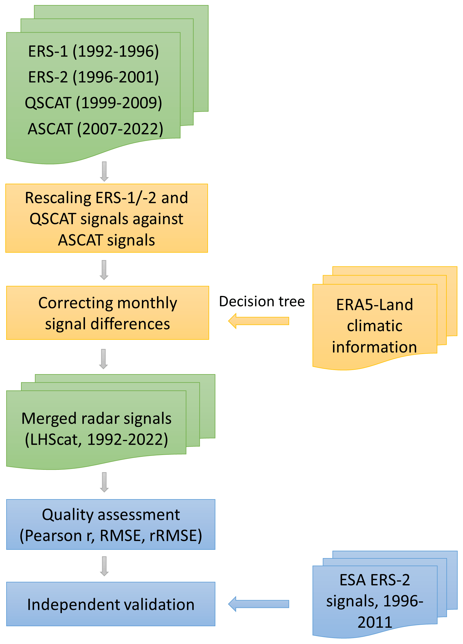
Figure 2Flow chart illustrating the development and assessment of the LHScat data set. Inputs/outputs are coloured in green, the signal-merging procedures coloured in yellow, and assessment and validation for the merged signals coloured in blue.
Regarding data rescaling, previous test beds have proposed two methods for rescaling time series, namely a linear regression correction (Brocca et al., 2011) and a cumulative density function (CDF) matching technique (Liu et al., 2009). The linear regression correction involves first scaling a time series within the range of the reference time series and then applying a linear regression equation between the two to minimize error. The CDF method further divides two time series into their quantile segments and then constructs a regression for each segment so that the CDF of a time series matches the CDF of the reference time series (Liu et al., 2009).
We found that the CDF method and the linear regression correction performed well in most regions (Fig. S1 in the Supplement). However, the CDF method failed in regions with a strong QSCAT signal trend, such as the deforested areas in southern Amazonia (Fig. 3a). This is mainly because QSCAT and ASCAT overlapped during 3 years, and the QSCAT signals in these 3 years do not cover the full signal range during 1999–2009. Linear regression correction, as used in Tao et al. (2022), is a preferable option to cope with this issue, but it is sensitive to sudden changes in radar signal (Fig. 3b). To overcome these limitations, we used the rescaling method illustrated in the following equation (Brocca et al., 2010, 2013; Draper et al., 2009):
where Qscaled indicates the scaled QSCAT signals, and Qoriginal means the original QSCAT signals prior to signal rescaling. Qmean_overlap and QSD_overlap indicate the mean and standardized deviation of the QSCAT signals with ASCAT in the overlapping period (i.e. 2007–2009). Likewise, Amean_overlap and ASD_overlap indicate the mean and standardized deviation of the ASCAT signals in the overlapping period.
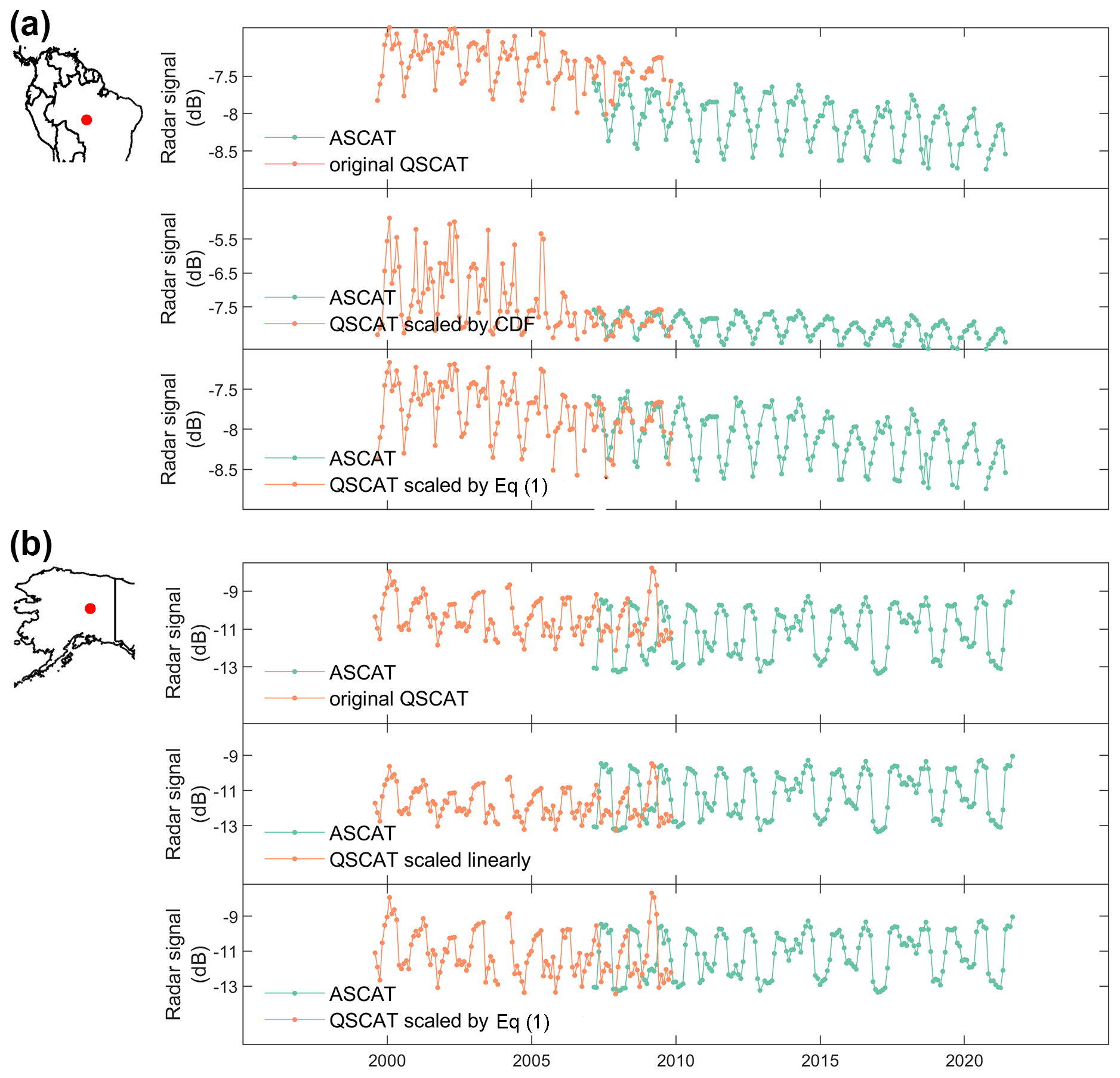
Figure 3Comparisons between the CDF method, the linear regression correction, and the method illustrated in Eq. (1) for rescaling radar signals. In most regions, the three methods performed almost equally well (Fig. S1), but the CDF method and the linear regression correction failed for signals with a strong trend or sudden changes. (a) Comparison between the CDF method and the method shown in Eq. (1) for rescaling a QSCAT signal time series with a strong decreasing trend. (b) Comparison between the linear regression correction and the method shown in Eq. (1) for rescaling a QSCAT signal time series with sudden increases in signal during the overlapping period.
This method has been used by previous research for rescaling soil moisture observations (Brocca et al., 2010, 2013; Draper et al., 2009). Here we found it to be robust to both the trends and sudden changes in radar signal (Fig. 3). We therefore used it to unify the scales of ERS-1/-2, QSCAT, and ASCAT signals. Specifically, monthly QSCAT signals were first scaled against monthly ASCAT signals, pixel by pixel. We chose ASCAT as the baseline for the rescaling because it has the best radiometric quality (lower sensitivity; higher radiometric resolution) and because it is still operational. Thereafter, ERS-2 signals were scaled against QSCAT signals (already scaled against ASCAT) using the same method. The ERS-1 and ERS-2 data sets were already calibrated, so there was no need to rescale them separately.
2.4 Addressing the monthly signal differences
Most existing research averaged the scaled signals directly to obtain a long-term merged time series (Du et al., 2017; Moesinger et al., 2020), but we here seek to correct the monthly signal differences before averaging the scaled signals. We previously found that the C-band and the scaled Ku-band signals exhibited large monthly differences in tropical regions (Tao et al., 2022). Importantly, the differences showed a seasonal pattern, with the Ku-band radar signal higher than C-band signal during the dry season and lower in the wet season. This phenomenon could be explained by the fact that the Ku-band signal has a shorter wavelength and lower penetrating ability relative to C-band and is thus more affected by tropical rainfall or intercepted water on leaf surfaces (Weissman et al., 2012; Prigent et al., 2022). To eliminate the signal differences, we first modelled the signal differences using rainfall as a predictor and then added the modelled signal differences to the Ku-band signal (Tao et al., 2022).
To extend our previous approach to the global scale, we explored the monthly signal difference against not only rainfall but also snow depth and skin temperature. Analogous to the effect of rainfall on Ku-band signals in tropical regions, we expect that snowpack prevents the Ku-band signal from reaching the land surface in regions covered by snow (Kelly et al., 2003; Naeimi et al., 2012). Skin temperature is related to a range of hydrological processes such as surface freeze/thaw, ice melting, and forest canopy evaporation (Konings et al., 2017). All of these could impact the radar signals by altering the water content of the measured objects. We therefore also expect skin temperature to be an effective predictor of the signal differences. Importantly, signal differences in many regions are caused by more than one climatic phenomenon. For instance, both precipitation and skin temperature could impact the Ku-band signals in forested regions through, respectively, rainfall contamination and canopy evaporation. In cold regions such as the Tibetan Plateau, precipitation, snow depth, and skin temperature could be jointly responsible for the signal differences, especially considering the hydrological process of rainfall–snow/ice formation–snow/ice melting (Fig. 4a).
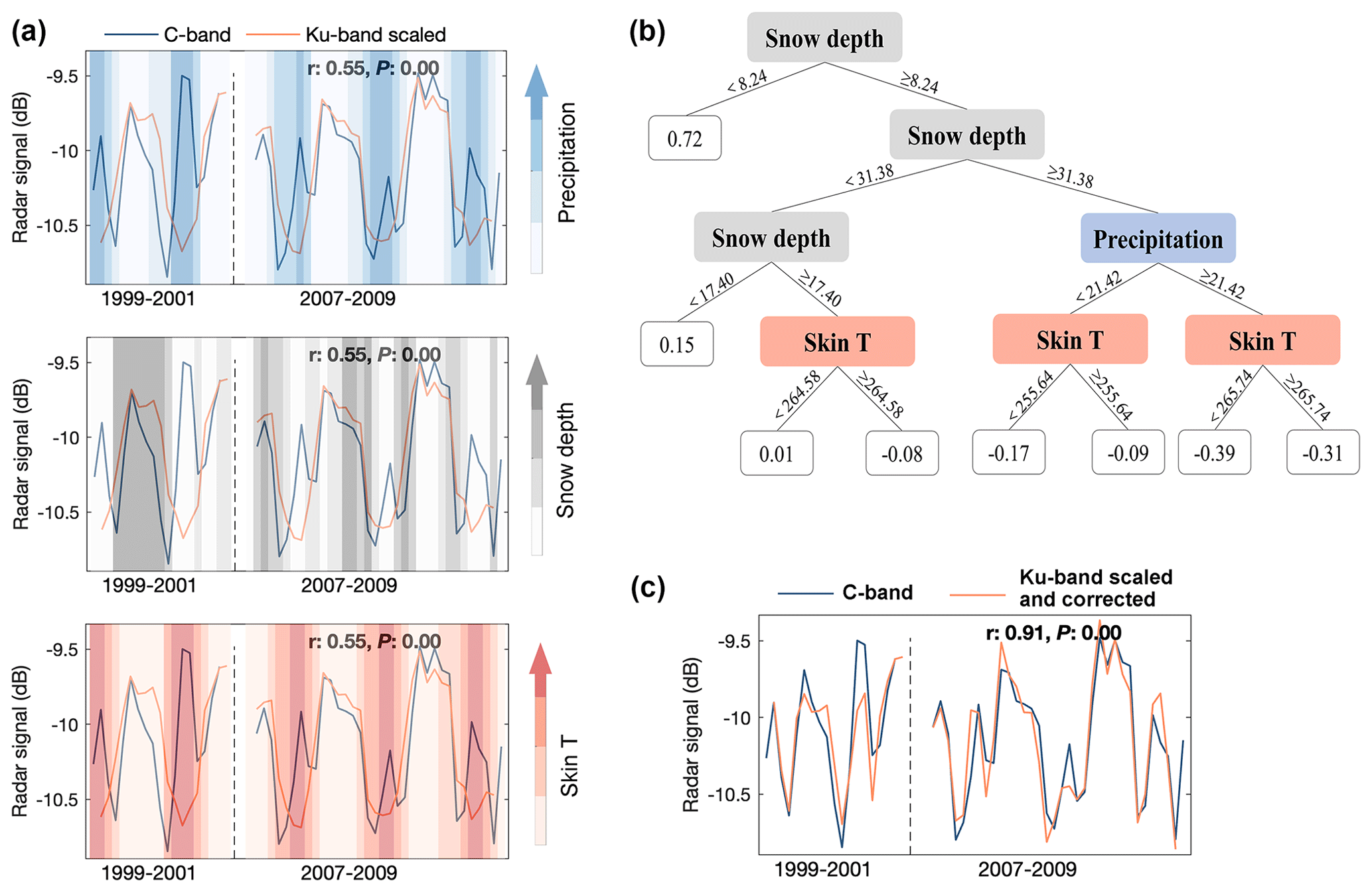
Figure 4Illustration on the correction of the monthly signal differences between the C-band and the scaled Ku-band signals in the overlapping years (1999–2001 and 2007–2009), taking 1 pixel in the Tibetan Plateau (88.01∘ E, 33.73∘ N) as an example. (a) The C-band and the scaled Ku-band signals before correction. The three panels in (a) show the radar signals against monthly precipitation (mm), skin temperature (K), and snow depth (mm). The vertical dotted line in each panel separates the ERS-QSCAT overlapping period (1999–2001) and QSCAT-ASCAT (2007–2009) overlapping period. (b) Decision tree regression with monthly precipitation, skin temperature, and snow depths as predictors of the signal differences. (c) The C-band and the final corrected Ku-band signals by the decision tree regression.
Thus, in order to model the signal differences from climatic variables accurately, we used decision tree regression. This technique recursively partitions observations into two sets based on a predictor that minimizes the predictive errors (Sankaran et al., 2005; Pekel, 2020). Compared with other modelling techniques, decision tree regression can be efficiently performed without a heavy computation burden. Besides, a major advantage of the decision tree regression is that it produces a model with easily interpretable rules (Sankaran et al., 2005; Loh, 2011). One example is shown in Fig. 4; while precipitation, skin temperature, and snow depth all contribute to the signal differences in 1 pixel of the Tibetan Plateau (Fig. 4a), the decision tree model clearly dissects the causes of the signal differences by creating binary trees first based on snow depth, then on precipitation, and finally on skin temperature (Fig. 4b). After the decision tree modelling, the Pearson r value between the C-band and Ku-band signals increases largely from 0.55 to 0.91 (Fig. 4c).
To summarize, combining monthly climatic variables and decision tree regression modelling, we corrected the monthly signal differences, pixel by pixel, using the following steps:
-
For each pixel, a decision tree regression model was built taking the monthly signal differences during the overlapping periods (i.e. 1999–2001, and 2007–2009) as a dependent variable and monthly ERA5-Land rainfall, snow depth, and skin temperature (0.1×0.1∘ resolution; Muñoz-Sabater, 2019) as explanatory variables. We used the MATLAB function fitrtree to implement the decision tree modelling (The MathWorks, Inc.).
-
After tree construction, cross-validation procedures were used to avoid overfitting. We increased the value for the MinLeafSize parameter from 1 to 30, with a step size of 1, and calculated the cross-validated errors. The MinLeafSize corresponding to the minimum cross-validated error was used, which ensures an optimal tree depth and a high predicative accuracy. Here, 5-fold cross-validation was used because only ∼60 overlapping observations (or ∼60 months) were available during 1999–2001 and 2007–2009, but we verified that the results were not altered with 10-fold cross-validation. The variable importance of the decision tree regression was quantified using the MATLAB function predictorImportance and the structure of the decision tree. While the former strictly computes the changes in predictive error due to splits for every predictor, the latter simply relies on the sequence of the predictors used to split the decision tree (i.e. the predictor used in the first split is the most important).
-
The decision tree regression model was then applied on climatic data from 1999 to 2009, and the predicted signal differences were added to the full QSCAT time series. In this way, the QSCAT signal was transformed into a substitute C-band signal.
-
After transforming the QSCAT data, we built a time series for each pixel for the 1992–2022 period, combining ERS-1/-2, QSCAT, and ASCAT time series. Radar observations from the overlapping periods (1999–2001 and 2007–2009) were averaged across sensors.
-
To assess the effectiveness of the data-merging approach, Pearson r (unitless), RMSE (dB), and relative RMSE (rRMSE; unitless) between the C-band and the corrected Ku-band signals in the overlapping periods (1999–2001 and 2007–2009) were finally calculated.
where denotes the mean of the monthly Ku-band signals x in the overlapping years, denotes the mean of the monthly C-band signals y in the overlapping years, xi and yi denote the values of x and y at the ith month, respectively, σy denotes the standard deviation of y, and n denotes the number of months in the overlapping years. rRMSE was used because it is normalized against the standard deviation of the signal and can therefore be compared across regions.
2.5 Validation of the data-merging approach
We also conducted a stricter evaluation of the data-merging approach. From January 2001 to 2011, the ERS-2 satellite experienced a series of failures that affected its data continuity and spatial coverage. However, observations were occasionally available for a subset of global pixels (Crapolicchio et al., 2012). This period overlaps with the QSCAT operating period; thus it can be used to test whether the corrected Ku-band (QSCAT) signal shows a consistent dynamic with the C-band signal. Recently, the European Space Agency (ESA) released the ERS-2 data set for the period of 2001–2011 reprocessed with the latest Advanced Scatterometer Processing System (ASPS) version 10.04 (Crapolicchio et al., 2012; https://earth.esa.int/eogateway/news/ers-1-scatterometer-l2-dataset-processed-with-asps-v10-04, last access: 4 April 2023). We used this version of ERS-2 data (hereafter referred to as ESA ERS-2) to validate our data-merging approach. Excluding Australia, Southern Africa, and the Bering Sea, 10 out of the 13 global regions were covered by the ESA ERS-2 data set during 2001 and 2011. For each of these 10 regions, we calculated monthly radar backscatter coefficients at 40∘ incidence angle from the ESA ERS-2 data set for comparison with our merged radar data set. To normalize the incidence angle, a linear regression was fitted between all incidence angles and the radar backscatter coefficients, and the R squared value and RMSE value of the regression were recorded. The backscatter coefficient at 40∘ incidence angle was then predicted by the regression. To ensure data quality, the predicted backscatter coefficient was not used if the RMSE was higher than 0.5 dB. Since the ESA ERS-2 data have a resolution of 25 km, we aggregated our merged radar signals to that resolution. For each month between 2001 and 2011, pixels with available ESA ERS-2 observations were located, and their ERS-2 signals were averaged across pixels. Because the footprints of the ESA ERS-2 observations are not fixed temporally, different months have a different subset of pixels. Our merged radar time series from the same pixels were then averaged and compared with the ESA ERS-2 signal mean. Months with too few pixels (<100) having ESA ERS-2 observations were not considered. This increases the strictness of the comparison in the sense that there is an additional spatial variation in pixels embedded within the radar time series.
3.1 Merged radar signals and quality assessments
The merged radar signal, averaged across pixels within a region, is presented in Fig. 5. Pearson r, RMSE, and rRMSE between the C-band and the corrected Ku-band signals in the overlapping years (1999–2001 and 2007–2009) were used to assess the quality of the merged radar signal. All 13 regions had a r value larger than 0.92, with a maximum of 0.99. We also obtained low RMSE values (from 0.05 to 0.11 dB), even in regions with a large seasonal amplitude in radar signal, such as Siberia, where the seasonal amplitude is around 3 dB but the RMSE is only 0.11 dB. This result was further confirmed by the low rRMSE values obtained in all regions, which ranged from 0.14 to 0.38.
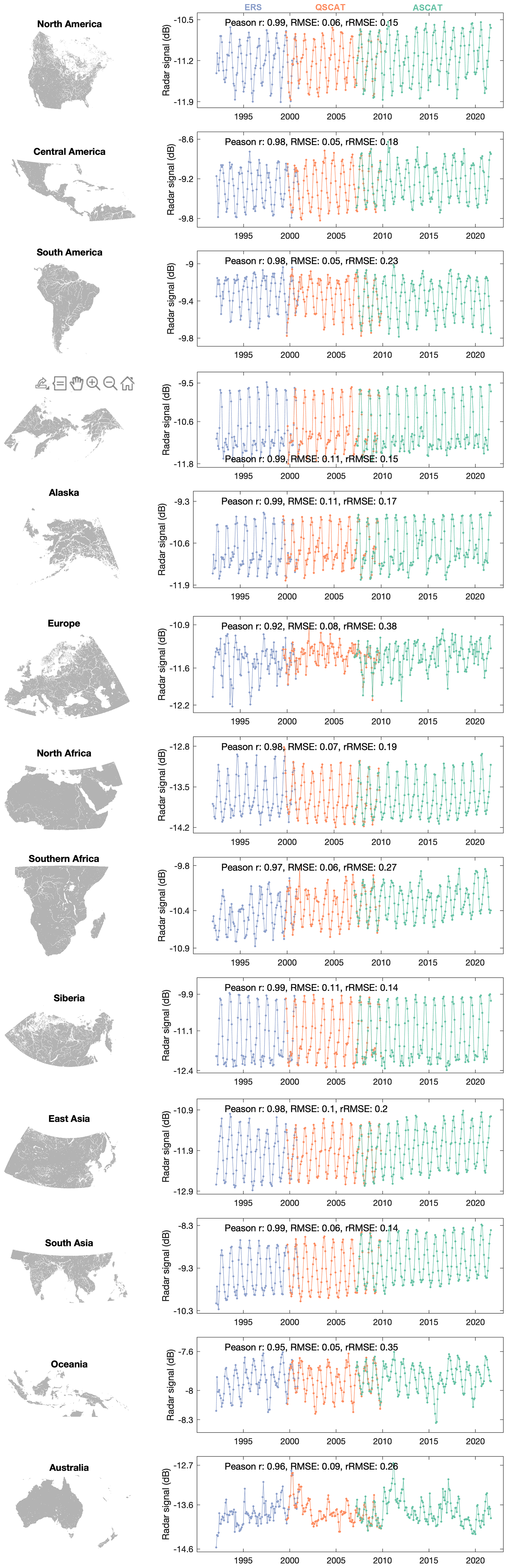
Figure 5Time series and quality assessment of the merged LHScat radar time series at the regional level. Each row shows one region. Inside each row, the map in the left panel shows the location of the region. The Lambert equal-area projection is used in the map. The line plot in the right panel shows the merged radar time series, averaged across pixels and coloured according to sensors. The Pearson r (unitless), RMSE (dB), and rRMSE (unitless) labelled in the panel were calculated using the C-band and the corrected Ku-band signals in the overlapping years (1999–2001 and 2007–2009) as indicators of the data-merging quality.
We further assessed the data-merging quality at the pixel level. Before correcting the monthly signal differences, the Pearson r values between the C-band and the scaled Ku-band signals showed a long-tailed distribution in all regions (Fig. 6). Regional median r values were relatively low, ranging from −0.22 to 0.91, and negative r values were found in almost all regions. After correcting the monthly signal differences, the regional median r values ranged from 0.64 to 0.94, with no negative r values observed (Fig. 6). The improvement was the most obvious in the northern high latitudes, such as Europe (r improved from 0.54 to 0.87), the Bering Sea (r from −0.13 to 0.94), Alaska (r from −0.16 to 0.94), and Siberia (r from −0.22 to 0.94). In contrast, the improvements for five regions, namely Central America, Australia, North Africa, South America, and South Asia, were relatively limited because their median r values prior to signal correction were already high. All of these five regions contain large portions of barren lands, deserts, shrublands, or grasslands, where the Ku-band signal is not as impacted as in forested and snow-covered regions.
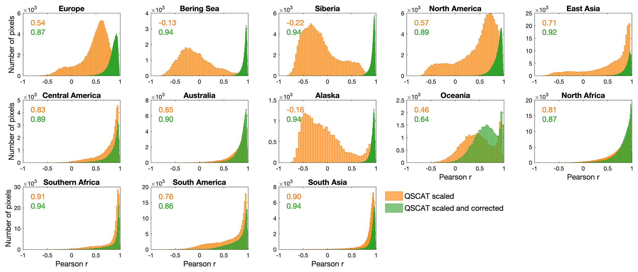
Figure 6Pearson r-based quality assessment of the LHScat data set at the pixel level. Each panel shows the result of one region. Inside each panel, the Pearson r values between the C-band and the scaled Ku-band signals in the overlapping years (1999–2001 and 2007–2009) were calculated for all pixels and coloured in orange. As a comparison, the Pearson r values between the C-band and the corrected Ku-band signals in the overlapping years were also calculated and coloured in green. The medians of the Pearson r values are labelled in each panel.
Regarding RMSE (Fig. 7), regional median RMSE values varied between 0.15 and 1.52 dB before the correction for signal differences but decreased sharply after the correction for signal differences (between 0.13 and 0.34 dB; Fig. 7). The most obvious improvement was still observed in the northern high latitudes such as Europe (RMSE decreased from 0.66 to 0.33 dB), the Bering Sea (RMSE from 1.32 to 0.31 dB), Alaska (RMSE from 1.28 to 0.31 dB), and Siberia (RMSE from 1.52 to 0.34 dB). Regional median rRMSE values were lower than 0.88, and in most regions lower than 0.5 (Fig. S2), consistent with the RMSE-based assessments. Besides, although rRMSE values were generally low in the final LHScat data set, tropical regions, mountainous regions, and arid regions had relatively higher rRMSE values than other regions (Fig. S3).
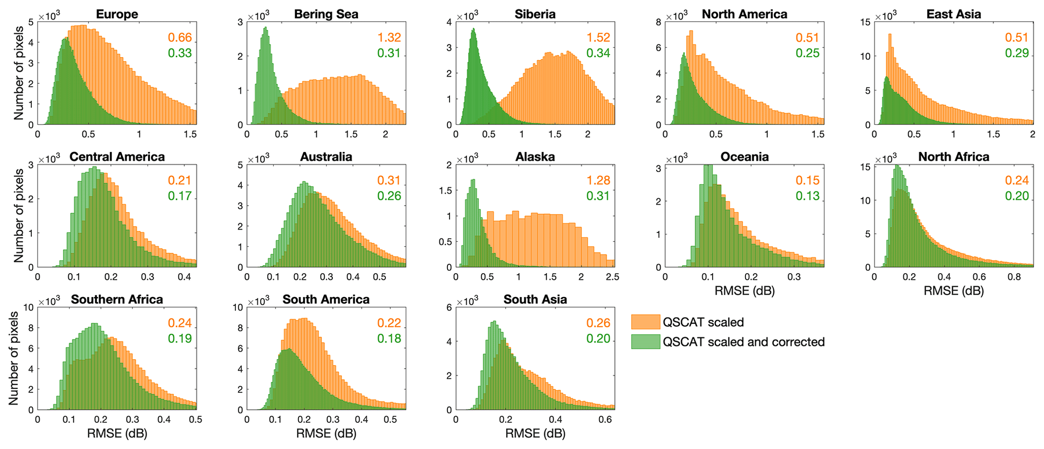
Figure 7RMSE-based quality assessment of the LHScat data set at the pixel level. Each panel shows the result of one region. Inside each panel, the RMSE values (dB) between the C-band and the scaled Ku-band signals in the overlapping years (1999–2001 and 2007–2009) were calculated for all pixels and coloured in orange. As a comparison, the RMSE values between the C-band and the corrected Ku-band signals in the overlapping years were also calculated and coloured in green. The medians of the RMSE values are labelled inside each panel. The rRMSE-based quality assessment is available in the Supplement (Figs. S2 and S3).
3.2 Importance of the predictor variables
We found that the most important predictors calculated by the MATLAB function predictorImportance (Fig. 8) were almost identical to the predictors used in the first splits of the decision trees (Fig. S4). We therefore illustrated the variable importance below, using the results presented in Fig. 8 (i.e. those calculated with predictorImportance). For 33.3 % of all the pixels, signal differences were most accurately predicted by rainfall (hereafter referred to as Type 1 pixels; Fig. 8). This type of pixel was mainly found in the Southern Hemisphere, particularly in tropical regions. In the Northern Hemisphere, such pixels were primarily located in the low and middle latitudes (Fig. 8).
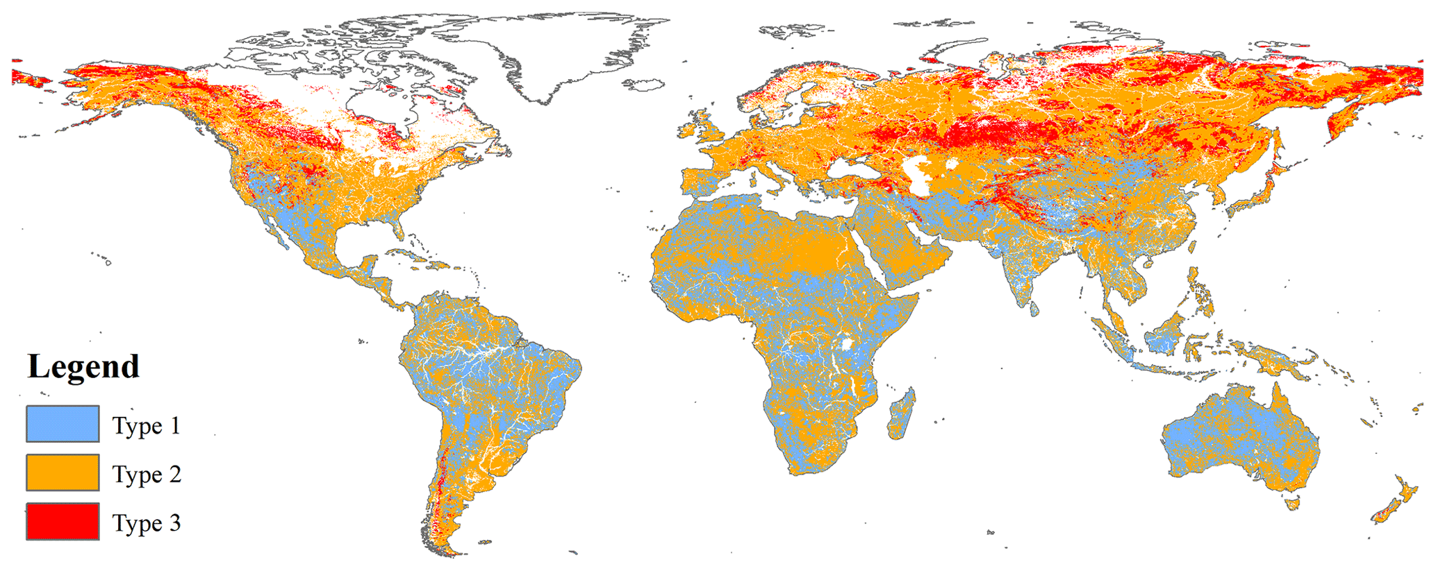
Figure 8Spatial distribution of variable importance for predicting the signal differences between the C-band and the scaled Ku-band signals in the overlapping years (1999–2001, 2007–2009). The variable importance was calculated from the decision tree regression model using the MATLAB function predictorImportance. For pixel Types 1, 2, and 3, the most important variables are monthly precipitation, skin temperature, and snow depth, respectively.
For 57.8 % of all the pixels, the signal differences were most accurately predicted by skin temperature (hereafter referred to as Type 2 pixels; Fig. 8). This type of pixel was widely distributed across the globe. In tropical regions, the spatial pattern of Type 2 pixels is similar to the pattern of Type 1 pixels (Fig. 8), which is expected because skin temperature and rainfall are correlated. The main differences between the distributions of Type 1 and Type 2 pixels were found in the northern high latitudes and dry regions, such as the hyper-arid Saharan and Arabian deserts.
Signal differences in the remaining 8.9 % pixels were most accurately predicted by snow depth (Fig. 8; hereafter referred to as Type 3 pixels). As expected, this type of pixel was primarily found in mountainous regions such as the Himalayas and the southern part of the Andes, as well as in the very high-latitude regions in the Northern Hemisphere.
3.3 Independent validation of the merged radar signal
The quality of the merged radar signals was also validated directly against the ESA ERS-2 data (see Sect. 2.5). The number of ESA ERS-2 pixels available for a comparison differed across regions. Furthermore, the pixel number decreased greatly in around 2003 in many regions (Fig. S5). Despite the variations in pixel number, we found highly similar monthly dynamics between the merged radar signals and the ESA ERS-2 signals in all regions. Using the Pearson r value as an index of similarity, all regions had a Pearson r value higher than 0.79, with a maximum of 0.98. Six regions had a r value higher than 0.90 (ranging from 0.90 to 0.98) (Fig. 9). This validation shows that the LHScat data are unlikely to be biased due to the cross-period merging method.
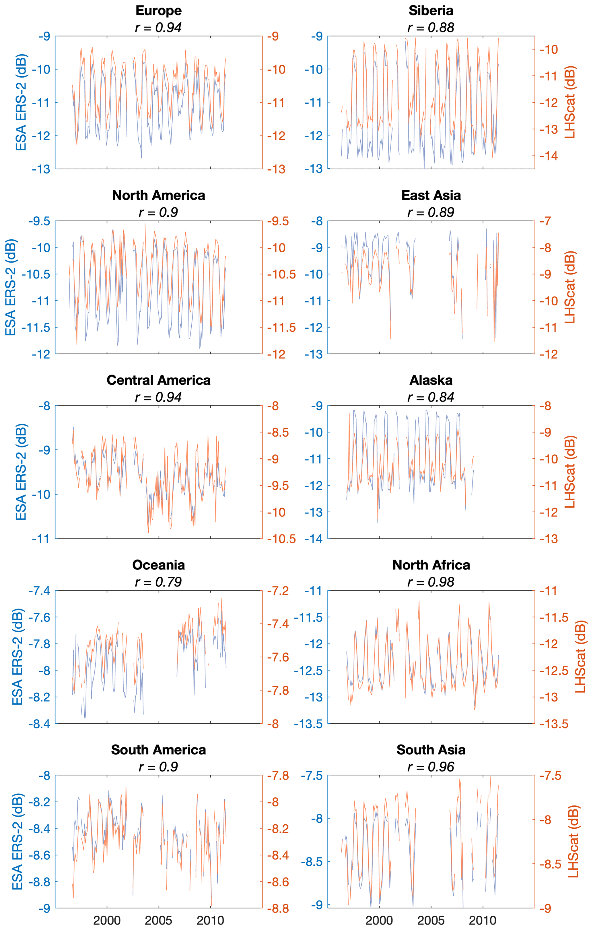
Figure 9Validation of the merged LHScat radar signals against the ESA ERS-2 data. Note that LHScat values are different from ESA ERS-2 values because the LHScat signals have been rescaled, taking ASCAT as the baseline.
The LHScat data set can be downloaded at https://doi.org/10.6084/m9.figshare.20407857 (Tao et al., 2023).
5.1 Rescaling the radar time series
The purpose of this project was to create the first global long-term radar backscatter data set with a consistent C-band signal dynamic. C-band ERS-1/-2 (1992–2001) and ASCAT (2007 onwards) signals were bridged by Ku-band QSCAT (1999–2009) signals. Observations overlapped between the three sensors, which allowed us to rescale the signal times series.
The CDF matching technique has been a classical signal rescaling method (Liu et al., 2009, 2011). For instance, Liu et al. (2011) used the CDF method for recalling the vegetation optical depth (VOD) derived from the Special Sensor Microwave/Imager (SSM/I; 1987–2007), Tropical Rainfall Measuring Mission (TRMM) Microwave Imager (TMI; 1998–2008), and AMSR-E (2002–2008) sensors. Moesinger et al. (2020) also used it for rescaling VOD products from SSM/I, AMSR-E, AMSR2 (2012–2019), and WindSat (2003–2012). In these previous studies, the overlapping periods among sensors are relatively long, with some even exceeding 10 years. In contrast, neither the ERS-2-QSCAT nor the QSCAT-ASCAT overlapping periods span more than 3 years. The rescaled QSCAT signals by CDF could therefore be biased, due, for instance, to deforestation in southern Amazonia (Fig. 3a). The linear regression correction can tackle this issue (Tao et al., 2022) but is sensitive to sudden changes in radar signal. As shown in Fig. 3b, the QSCAT signal surged in 2009 in one location of Alaska, and the linear regression correction created an obvious bias in the rescaled QSCAT signals. This situation is rare in tropical regions but appears more frequent in northern high latitudes, possibly due to the surface freeze–thaw process. Although we have excluded potential outliers from the radar signals by implementing a standard deviation filter (see Sect. 2.2), such sudden changes were not identified as outliers.
We used a simple yet effective method for rescaling the signal time series. This method is rooted in the discipline of statistics and has been used successfully by previous research for rescaling soil moisture data (Brocca et al., 2010, 2013; Draper et al., 2009). We here further demonstrated its capability of rescaling microwave signals with a short overlapping period (∼3 years). Additionally, the results shown in Fig. 3 suggest that this method is robust in response to both the trends and sudden changes in the radar signal. Merging the time series of satellite observations has been an important yet challenging task in Earth science studies. Many sensors have temporal overlaps, such as among AMSR-E, ASCAT, Sentinel-1, and SMOS, with the lengths of overlapping period ranging from several months to a couple of years (Table 1). Rescaling these data using Eq. (1) could uncover interesting mechanisms underlying the signal differences, which is an important prerequisite for creating data sets with an even longer time span.
5.2 Signal quality and merging mechanism
After rescaling the radar time series from different sensors, monthly signal differences were corrected by modelling them from climatic variables (namely precipitation, skin temperature, and snow depth). The quality of the merged radar signals was assessed against the ESA ERS-2 data set. Highly similar monthly time series were obtained, suggesting high accuracy for the merging procedure.
Why did rainfall, skin temperature, and snow depth successfully predict the signal differences? The main reason is that the Ku-band signal has a lower penetrating ability in comparison to the C-band signal because of its shorter wavelength. In regions with a strong rainfall, such as the tropics, Ku-band signals are more impacted by raindrops and the intercepted water on leaf surfaces, thus showing different seasonal patterns with C-band signals (Fig. 4a). The rainfall attenuation of high-frequency microwave signals (Ku/Ka band or GHz) is used for microwave-derived rain retrieval, such as for the case of precipitation radar operating at 13.8 GHz on board TRMM (Iguchi et al., 2000).
Skin temperature is found to be an effective predictor of the signal differences for 57.8 % of all pixels (Fig. 8). This is expected because skin temperature not only correlates with rainfall but also reflects several land surface processes. In tropical regions, skin temperature was found as an almost equally important predictor of signal difference as rainfall. The first explanation for this result is that there is a negative correlation between skin temperature and rainfall in tropical regions. A second explanation could be the increased evapotranspiration of the rainforest canopy in dry periods due to high vapour pressure deficit. Increased evapotranspiration is correlated with skin temperature and could impact the Ku-band signals, thus influencing the top canopy moisture. This phenomenon therefore helps to explain why Ku-band signals are higher than C-band signals in dry periods (Guan et al., 2015; Konings et al., 2017).
In boreal regions (Fig. 8), skin temperature is also an effective predictor of the signal differences. This could be related to the fact that the local land surfaces in these regions are seasonally frozen, or covered by ice, thus causing different signal performances between Ku-band and C-band signals. The surface freeze–thaw cycle is captured by skin temperature changes, explaining why there is a skin-temperature-predicted signal difference in these regions.
In arid regions such as the Saharan and Arabian deserts (Fig. 8), skin temperature also explained the signal differences in most pixels. These regions receive limited amount of rainfall annually. Soil moisture is therefore mainly controlled by land surface processes, such as the seasonal changes in wind intensity/direction in deserts, which modify the roughness of the sand dunes and finally lead to a temporal variation in soil moisture (Frappart et al., 2015). Soil moisture changes with skin temperature, leading to changes in the penetration depths of C-band and Ku-band signals, due to the attenuation of the microwave signal as a function of moisture. This hypothesis could explain why skin temperature is closely related to the signal differences in some arid regions.
Snow depth was found to be the most effective predictor of the signal differences in mountainous and high-latitude regions seasonally covered by snow. The Ku-band signal interacts with snow because of its short wavelength; thus its dynamics follow the seasonal changes in snow depth. The Ku-band signal is higher when snow depth is deeper, and vice versa (Fig. 4a), but the C-band signal shows the opposite dynamic, possibly because of a deeper penetration. In fact, this phenomenon has long been recognized by classical research which models snow depth or snow water equivalent from microwave signal differences (Kelly et al., 2003). Since the launch of Scanning Multichannel Microwave Radiometer (SMMR) in 1978, microwave data have been used to estimate snow depth and snow water equivalent. One of the classical methods is based on the fact that microwaves at different frequencies respond differently to snow cover. For instance, the Chang et al. (1982) equation utilizes the channel differences between low- (such as 19 GHz) and high- (such as 37 GHz) frequency brightness temperatures observed by passive microwave sensors. Here, we found similar signal differences between low- (C-band) and high- (Ku-band) frequency radar signals. Since several radar sensors at different frequencies are operating, efforts could be made to create products of snow depth or snow water equivalent by combining radar signals of different frequencies such as QSCAT and ASCAT.
It is also worth noting that, although climatic data were used to merge radar signals into a single time series, this does not mean that our final radar signals contain mainly climate information. The three climatic variables were merely used to model signal differences, which were then added to the Ku-band signals. Besides, the 1999–2009 period accounts for only a third of the entire time span. Thus, the main information contained in the merged signals is related to features of the land surface rather than to climate.
5.3 Limitations and future works
We used the reanalysis ERA5-Land monthly climatic data to model the signal differences. As a result, whether signal differences can be accurately modelled partly depends on the accuracy of the ERA5-Land climatic data. Future work will test the effectiveness of other climatic data sets for modelling the signal differences. The accurate mapping of some climatic variables, such as snow depth, is challenging (Orsolini et al., 2019; Clifford, 2010; Pulliainen et al., 2020). This is critical in the high-latitude regions such as northern Alaska, where snow depth is the most important variable predicting the signal differences. The estimation of rainfall is also challenging in regions with sparse climate stations such as the tropics. An increasing number of climate data sets has been made publicly available, including the Modern-Era Retrospective analysis for Research and Applications, version 2 (MERRA-2; Gelaro et al., 2017), and the Climate Hazards Group InfraRed Precipitation with Station data (CHIRPS). The snow depth product of MERRA-2 has been demonstrated as being superior to ERA5 in mainland China (Zhang et al., 2021). The CHIRPS precipitation was also validated to have an excellent performance in tropical Africa (Camberlin et al., 2019). Thus, it is possible that these climate products may produce a better merging quality for tropical and mountainous regions where the rRMSE values remained relatively high (Fig. S3).
Except for climatic layers, remote-sensing-based layers such as the normalized difference vegetation index (NDVI) could be useful for modelling the signal differences in vegetated areas. NDVI reflects the vegetation growth condition, which is the result of several environmental factors interacting. NDVI therefore contains kinds of multiple environmental information. In addition, aerosol could be a contributing factor to the signal differences, especially in deserts such as the Sahara, where the rRMSE values in the final LHScat data set remained relatively high (Fig. S3). The Sentinel-5P mission provides near-real-time, high-resolution aerosol products starting from the year 2018 (Ingmann et al., 2012). Analysis will soon be conducted to assess whether NDVI and aerosol layers can further improve the data-merging quality.
Another potentially useful data set to be included into our data-merging framework is the Oceansat-2 scatterometer (OSCAT). OSCAT also provides Ku-band backscatters akin to QSCAT but operating in a different period (between 2009 and 2014; Bhowmick et al., 2013). QSCAT operated in full mode between 1999 and 2009 and overlapped with ASCAT during 3 years (2007–2009). Adding OSCAT will expand the overlapping period by 5 years (up to 2014), which could help further improve the data-merging method.
In Tao et al. (2022), linear regression was established to predict the signal differences from monthly rainfall amounts because the signal differences exhibited a good linear relationship with rainfall in tropical rainforest regions. Decision tree regression was also adopted in Tao et al. (2022) for a limited number of pixels mainly located in the ever-wet northwestern Amazonian and Asian tropical rainforests. This is because the relationship between signal differences and rainfall in these ever-wet regions is nonlinear. The present study used only the decision tree regression (Fig. 4) and used three climatic variables to increase the modelling accuracy. More advanced machine learning techniques are an option in the future.
The LHScat data set currently has a spatial resolution of 8.9 km, which is much higher than the ∼25 km resolution of previous microwave data sets (Liu et al., 2011; Moesinger et al., 2020). This was achieved partly by reducing the temporal resolution, since the SIRF algorithm requires multiple-orbit satellite passes to obtain a fine spatial resolution (Long et al., 1993; Early and Long, 2001). We further composited the images into a monthly temporal resolution for facilitating global-scale studies, such as global vegetation biomass and soil moisture estimations. However, we acknowledge that the monthly temporal resolution might be less useful for local-scale studies requiring frequent observations such as phenological monitoring (Pfeil et al., 2020). New versions of LHScat with even higher spatial and temporal resolutions are being created using the methodology developed in this study. Higher spatial resolution can be achieved by merging only QSCAT and ASCAT images. As stated in the introduction to this paper, the BYU data centre provides QSCAT and ASCAT images at the resolution of 4.45 km. It is therefore possible to generate a global C-band radar data set at 4.45 km resolution but with a shorter time span (since the QSCAT mission started in 1999). It is also possible to have higher temporal resolutions, such as time-averaged (such as weekly) resolutions (Lin et al., 2016). New versions of LHScat will be made publicly available at https://doi.org/10.6084/m9.figshare.20407857.
C-band radar data have been widely used in Earth science studies for monitoring vegetation dynamics, mapping deforestation and soil moisture, and estimating snow water equivalent (Chang et al., 1982; Clifford, 2010; Kelly et al., 2003; Liu et al., 2009; Saatchi et al., 2013; Steele-Dunne et al., 2017; Smith and Bookhagen, 2018). Thus, the merged radar signals are expected to be useful in a range of research disciplines. A possible outcome is to separate the signal into soil moisture and vegetation optical depth (VOD). In this way, the signals can be more directly related to the soil or vegetation dynamics. Technically, extracting VOD and soil moisture from LHScat signal is feasible with the help of the Water Cloud Model (Liu et al., 2021), and efforts are being devoted to developing a LHScat VOD data set at the global scale. Considering its long time span (since 1992) and high resolution, LHScat VOD would be suitable for the assessment of long-term global vegetation changes. Using the optical Moderate Resolution Imaging Spectroradiometer (MODIS) leaf area index data, a recent study found that most of the world's vegetated areas are becoming greener, particularly in China and India (Chen et al., 2019). Using the optical vegetation index NDVI, another recent research explored the long-term (2000–2020) resilience change in global forests (Forzieri et al., 2022). It would be interesting to re-evaluate the vegetation trends using LHScat VOD data. While radar signal penetrates the upper forest canopy and interacts directly with the water molecules contained in forest biomass, optical greenness data reflect the canopy features of the top-most leaf layer which could be maintained due to leaf demography or light availability (Guan et al., 2015; Wu et al., 2016). We therefore expect the LHScat VOD to provide new insights into the long-term changes in global forests.
The supplement related to this article is available online at: https://doi.org/10.5194/essd-15-1577-2023-supplement.
ST, AZ, and YL designed the research. ST and AZ analysed the data, with input from other authors. ST, JPW, SSa, PC, JC, TL, and PLF wrote the paper. All authors interpreted the results and edited the text.
The contact author has declared that none of the authors has any competing interests.
Publisher's note: Copernicus Publications remains neutral with regard to jurisdictional claims in published maps and institutional affiliations.
We thank the BYU data centre and David Long for providing the enhanced-resolution radar images.
This research has been supported by the National Natural Science Foundation of China (grant no. 31988102), the Chinese Academy of Sciences (grant no. XDA26010303), ESA (CCI-BIOMASS), and the Agence Nationale de la Recherche (CEBA, grant no. ANR-10-LABX-25-01; TULIP, grant no. ANR-10-LABX-0041; ANAEE-France, grant no. ANR-11-INBS-0001).
This paper was edited by Jing Wei and reviewed by three anonymous referees.
Attema, E., Desnos, Y. L., and Duchossois, G.: Synthetic aperture radar in Europe: ERS, Envisat, and beyond, Johns Hopkins APL technical digest, 21, 155–161, 2000.
Bentamy, A., Grodsky, S. A., Carton, J. A., Croizé-Fillon, D., and Chapron, B.: Matching ASCAT and QuikSCAT winds, J. Geophys. Res.-Oceans, 117, 1–15, 2012.
Bhowmick, S. A., Kumar, R., and Kumar, A. K.: Cross calibration of the OceanSAT-2 scatterometer with QuikSCAT scatterometer using natural terrestrial targets, IEEE T. Geosci. Remote, 52, 3393–3398, 2013.
Brocca, L., Melone, F., Moramarco, T., Wagner, W., Naeimi, V., Bartalis, Z., and Hasenauer, S.: Improving runoff prediction through the assimilation of the ASCAT soil moisture product, Hydrol. Earth Syst. Sci., 14, 1881–1893, https://doi.org/10.5194/hess-14-1881-2010, 2010.
Brocca, L., Hasenauer, S., Lacava, T., Melone, F., Moramarco, T., Wagner, W., Dorigo, W., Matgen, P., Martínez-Fernández, J., and Llorens, P.: Soil moisture estimation through ASCAT and AMSR-E sensors: An intercomparison and validation study across Europe, Remote Sens. Environ., 115, 3390-3408, 2011.
Brocca, L., Melone, F., Moramarco, T., Wagner, W., and Albergel, C.: Scaling and filtering approaches for the use of satellite soil moisture observations, in: Remote Sensing of Energy Fluxes and Soil Moisture Content, 1st Edn., edited by: Petropoulos, G., CRC Press, Boca Raton, Florida, USA, 411–426, ISBN 9780429096549, 2013.
Camberlin, P., Barraud, G., Bigot, S., Dewitte, O., Makanzu Imwangana, F., Maki Mateso, J. C., Martiny, N., Monsieurs, E., Moron, V., and Pellarin, T.: Evaluation of remotely sensed rainfall products over Central Africa, Q. J. Roy. Meteorol. Soc., 145, 2115–2138, 2019.
Carabajal, C. C. and Harding, D. J.: SRTM C-band and ICESat laser altimetry elevation comparisons as a function of tree cover and relief, Photogram. Eng. Remote Sens., 72, 287–298, 2006.
Chang, A. T., Foster, J. L., Hall, D. K., Rango, A., and Hartline, B. K.: Snow water equivalent estimation by microwave radiometry, Cold Reg. Sci. Technol., 5, 259–267, 1982.
Chen, C., Park, T., Wang, X., Piao, S., Xu, B., Chaturvedi, R. K., Fuchs, R., Brovkin, V., Ciais, P., and Fensholt, R.: China and India lead in greening of the world through land-use management, Nat. Sustain., 2, 122–129, 2019.
Clifford, D.: Global estimates of snow water equivalent from passive microwave instruments: history, challenges and future developments, Int. J. Remote Sens., 31, 3707–3726, 2010.
Crapolicchio, R., and Lecomte, P.: On the Stability of Amazon rain forest backscattering during the ERS-2 Scatterometer mission lifetime, in: Proceeding of ASAR Workshop 2003, Canadian Space Agency Saint-Hubert, Quebec, https://citeseerx.ist.psu.edu/document?repid=rep1&type=pdf&doi=e7a3d4abb6c1aef0d89ca778f5ef9292a5d4070d (last access: 9 April 2023), 2003.
Crapolicchio, R., De Chiara, G., Elyouncha, A., Lecomte, P., Neyt, X., Paciucci, A., and Talone, M.: ERS-2 scatterometer: Mission performances and current reprocessing achievements, IEEE T. Geosci. Remote, 50, 2427–2448, 2012.
Draper, C. S., Walker, J. P., Steinle, P. J., De Jeu, R. A., and Holmes, T. R.: An evaluation of AMSR-E derived soil moisture over Australia, Remote Sens. Environ., 113, 703–710, 2009.
Du, J., Kimball, J. S., Jones, L. A., Kim, Y., Glassy, J., and Watts, J. D.: A global satellite environmental data record derived from AMSR-E and AMSR2 microwave Earth observations, Earth Syst. Sci. Data, 9, 791–808, https://doi.org/10.5194/essd-9-791-2017, 2017.
Early, D. S. and Long, D. G.: Image reconstruction and enhanced resolution imaging from irregular samples, IEEE T. Geosci. Remote, 39, 291–302, 2001.
ESA: Mission ends for Copernicus Sentinel-1B satellite, https://www.esa.int/Applications/Observing_the_Earth/Copernicus/Sentinel-1/Mission_ends_for_Copernicus_Sentinel-1B_satellite (last access: 20 January 2023), 2022.
Figa-Saldaña, J., Wilson, J. J., Attema, E., Gelsthorpe, R., Drinkwater, M. R., and Stoffelen, A.: The advanced scatterometer (ASCAT) on the meteorological operational (MetOp) platform: A follow on for European wind scatterometers, Can. J. Remote Sens., 28, 404–412, 2002.
Forzieri, G., Dakos, V., McDowell, N. G., Ramdane, A., and Cescatti, A.: Emerging signals of declining forest resilience under climate change, Nature, 608, 534–539, 2022.
Frappart, F., Fatras, C., Mougin, E., Marieu, V., Diepkilé, A., Blarel, F., and Borderies, P.: Radar altimetry backscattering signatures at Ka, Ku, C, and S bands over West Africa, Phys. Chem. Earth, 83, 96–110, 2015.
Frison, P.-L. and Mougin, E.: Use of ERS-1 wind scatterometer data over land surfaces, IEEE Trans. Geosci. Remote, 34, 550–560, 1996.
Frolking, S., Milliman, T., Mahtta, R., Paget, A., Long, D. G., and Seto, K. C.: A global urban microwave backscatter time series data set for 1993–2020 using ERS, QuikSCAT, and ASCAT data, Sci. Data, 9, 1–12, 2022a.
Frolking, S., Mahtta, R., Milliman, T., and Seto, K. C.: Three decades of global trends in urban microwave backscatter, building volume and city GDP, Remote Sens. Environ., 281, 113225, https://doi.org/10.1016/j.rse.2022.113225, 2022b.
Gelaro, R., McCarty, W., Suárez, M. J., Todling, R., Molod, A., Takacs, L., Randles, C. A., Darmenov, A., Bosilovich, M. G., and Reichle, R.: The modern-era retrospective analysis for research and applications, version 2 (MERRA-2), J. Climate, 30, 5419–5454, 2017.
Guan, K., Pan, M., Li, H., Wolf, A., Wu, J., Medvigy, D., Caylor, K. K., Sheffield, J., Wood, E. F., and Malhi, Y.: Photosynthetic seasonality of global tropical forests constrained by hydroclimate, Nat. Geosci., 8, 284–289, 2015.
Hilburn, K. A. and Wentz, F. J.: Mitigating the impact of RADCAL beacon contamination on F15 SSM/I ocean retrievals, Geophys. Res. Lett., 35, L18806, https://doi.org/10.1029/2008GL034914, 2008.
Hollinger, J. P., Peirce, J. L., and Poe, G. A.: SSM/I instrument evaluation, IEEE T. Geosci. Remote, 28, 781–790 1990.
Iguchi, T., Kozu, T., Meneghini, R., Awaka, J., and Okamoto, K. I.: Rain-profiling algorithm for the TRMM precipitation radar, J. Appl. Meteorol., 39, 2038–2052, 2000.
Ingmann, P., Veihelmann, B., Langen, J., Lamarre, D., Stark, H., and Courrèges-Lacoste, G. B.: Requirements for the GMES Atmosphere Service and ESA's implementation concept: Sentinels-4/-5 and-5p, Remote Sens. Environ., 120, 58–69, 2012.
Kelly, R. E., Chang, A. T., Tsang, L., and Foster, J. L.: A prototype AMSR-E global snow area and snow depth algorithm, IEEE T. Geosci. Remote, 41, 230–242, 2003.
Konings, A. G., Yu, Y., Xu, L., Yang, Y., Schimel, D. S., and Saatchi, S. S.: Active microwave observations of diurnal and seasonal variations of canopy water content across the humid African tropical forests, Geophys. Res. Lett., 44, 2290–2299, 2017.
Kummerow, C., Simpson, J., Thiele, O., Barnes, W., Chang, A. T. C., Stocker, E., Adler, R. F., Hou, A., Kakar, R., Wentz, F., Ashcroft, P., Kozu, T., Hong, Y., Okamoto, K., Iguchi, T., Kuroiwa, H., Im, E., Haddad, Z., Huffman, G., Ferrier, B., Olson, W. S., Zipser, E., Smith, E. A., Wilheit, T. T., North, G., Krishnamurti, T., and Nakamura, K.: The Status of the Tropical Rainfall Measuring Mission (TRMM) after Two Years in Orbit, J. Appl. Meteorol., 39, 1965–1982, 2000.
Le Toan, T., Quegan, S., Davidson, M., Balzter, H., Paillou, P., Papathanassiou, K., Plummer, S., Rocca, F., Saatchi, S., and Shugart, H.: The BIOMASS mission: Mapping global forest biomass to better understand the terrestrial carbon cycle, Remote Sens. Environ., 115, 2850–2860, 2011.
Lin, C. C., Lengert, W., and Attema, E.: Three generations of C-band wind scatterometer systems from ERS-1/2 to MetOp/ASCAT, and MetOp second generation, IEEE J. Select. Top. Appl. Earth Obs. Remote Sens., 10, 2098–2122, 2016.
Liu, X., Wigneron, J.-P., Fan, L., Frappart, F., Ciais, P., Baghdadi, N., Zribi, M., Jagdhuber, T., Li, X., and Wang, M.: ASCAT IB: A radar-based vegetation optical depth retrieved from the ASCAT scatterometer satellite, Remote Sens. Environ., 264, 112587, https://doi.org/10.1016/j.rse.2021.112587, 2021.
Liu, Y. Y., van Dijk, A. I., de Jeu, R. A., and Holmes, T. R.: An analysis of spatiotemporal variations of soil and vegetation moisture from a 29-year satellite-derived data set over mainland Australia, Water Resour. Res., 45, W07405, https://doi.org/10.1029/2008WR007187, 2009.
Liu, Y. Y., De Jeu, R. A., McCabe, M. F., Evans, J. P., and Van Dijk, A. I.: Global long-term passive microwave satellite-based retrievals of vegetation optical depth, Geophys. Res. Lett., 38, L18402, https://doi.org/10.1029/2011GL048684, 2011.
Loh, W. Y.: Classification and regression trees, Wiley Interdisciplin. Rev.: Data Min. Knowl. Discov., 1, 14–23, 2011.
Long, D. G., Hardin, P. J., and Whiting, P. T.: Resolution enhancement of spaceborne scatterometer data, IEEE T. Geosci. Remote, 31, 700–715, 1993.
Malenovský, Z., Rott, H., Cihlar, J., Schaepman, M. E., García-Santos, G., Fernandes, R., and Berger, M.: Sentinels for science: Potential of Sentinel-1,-2, and -3 missions for scientific observations of ocean, cryosphere, and land, Remote Sens. Environ., 120, 91–101, 2012.
Moesinger, L., Dorigo, W., de Jeu, R., van der Schalie, R., Scanlon, T., Teubner, I., and Forkel, M.: The global long-term microwave Vegetation Optical Depth Climate Archive (VODCA), Earth Syst. Sci. Data, 12, 177–196, https://doi.org/10.5194/essd-12-177-2020, 2020.
Muñoz-Sabater, J.: ERA5-Land monthly averaged data from 1981 to present, Copernicus Climate Change Service (C3S) Climate Data Store (CDS) [data set], https://doi.org/10.24381/cds.68d2bb30, 2019.
Murfitt, J. and Duguay, C. R.: 50 years of lake ice research from active microwave remote sensing: Progress and prospects, Remote Sens. Environ., 264, 112616, https://doi.org/10.1016/j.rse.2021.112616, 2021.
Naeimi, V., Paulik, C., Bartsch, A., Wagner, W., Kidd, R., Park, S.-E., Elger, K., and Boike, J.: ASCAT Surface State Flag (SSF): Extracting information on surface freeze/thaw conditions from backscatter data using an empirical threshold-analysis algorithm, IEEE T. Geosci. Remote, 50, 2566–2582, 2012.
NCAR Climate data guide: QuikSCAT: near sea-surface wind speed and direction, https://climatedataguide.ucar.edu/climate-data/quikscat-near-sea-surface-wind-speed-and-direction, last access: 20 January 2023.
NSIDC: AMSR-E Instrument Failure, https://nsidc.org/data/user-resources/data-announcements/amsr-e-instrument-failure (last access: 20 January 2023), 2011.
Orsolini, Y., Wegmann, M., Dutra, E., Liu, B., Balsamo, G., Yang, K., de Rosnay, P., Zhu, C., Wang, W., Senan, R., and Arduini, G.: Evaluation of snow depth and snow cover over the Tibetan Plateau in global reanalyses using in situ and satellite remote sensing observations, The Cryosphere, 13, 2221–2239, https://doi.org/10.5194/tc-13-2221-2019, 2019.
Pekel, E.: Estimation of soil moisture using decision tree regression, Theor. Appl. Climatol., 139, 1111–1119, 2020.
Pfeil, I., Wagner, W., Forkel, M., Dorigo, W., and Vreugdenhil, M.: Does ASCAT observe the spring reactivation in temperate deciduous broadleaf forests?, Remote Sens. Environ., 250, 112042, https://doi.org/10.1016/j.rse.2020.112042, 2020.
Prigent, C., Matthews, E., Aires, F., and Rossow, W. B.: Remote sensing of global wetland dynamics with multiple satellite data sets, Geophys. Res. Lett., 28, 4631–4634, 2001.
Prigent, C., Jimenez, C., Dinh, L. A., Frappart, F., Gentine, P., Wigneron, J. P., and Munchak, J.: Diurnal and Seasonal Variations of Passive and Active Microwave Satellite Observations Over Tropical Forests, J. Geophys. Res.-Biogeo., 127, e2021JG006677, https://doi.org/10.1029/2021JG006677, 2022.
Pulliainen, J., Luojus, K., Derksen, C., Mudryk, L., Lemmetyinen, J., Salminen, M., Ikonen, J., Takala, M., Cohen, J., and Smolander, T.: Patterns and trends of Northern Hemisphere snow mass from 1980 to 2018, Nature, 581, 294–298, 2020.
Saatchi, S., Asefi-Najafabady, S., Malhi, Y., Aragão, L. E., Anderson, L. O., Myneni, R. B., and Nemani, R.: Persistent effects of a severe drought on Amazonian forest canopy, P. Natl. Acad. Sci. USA, 110, 565–570, 2013.
Sankaran, M., Hanan, N. P., Scholes, R. J., Ratnam, J., Augustine, D. J., Cade, B. S., Gignoux, J., Higgins, S. I., Le Roux, X., and Ludwig, F.: Determinants of woody cover in African savannas, Nature, 438, 846–849, 2005.
Shi, J., Xiong, C., and Jiang, L.: Review of snow water equivalent microwave remote sensing, Sci. China Earth Sci., 59, 731–745, 2016.
Smith, T. and Bookhagen, B.: Changes in seasonal snow water equivalent distribution in High Mountain Asia (1987 to 2009), Sci. Adv., 4, e1701550, https://doi.org/10.1126/sciadv.1701550, 2018.
Spreen, G., Kaleschke, L., and Heygster, G.: Sea ice remote sensing using AMSR-E 89-GHz channels, J. Geophys. Res.-Oceans, 113, C02S03, https://doi.org/10.1029/2005JC003384, 2008.
Steele-Dunne, S. C., McNairn, H., Monsivais-Huertero, A., Judge, J., Liu, P.-W., and Papathanassiou, K.: Radar remote sensing of agricultural canopies: A review, IEEE J. Select. Top. Appl. Earth Obs. Remote Sens., 10, 2249–2273, 2017.
Sun, Q., Miao, C., Duan, Q., Ashouri, H., Sorooshian, S., and Hsu, K. L. A review of global precipitation data sets: Data sources, estimation, and intercomparisons, Rev. Geophys., 56, 79–107, 2018.
Tao, S., Chave, J., Frison, P.-L., Toan, T. L., Ciais, P., Fang, J., Wigneron, J.-P., Santoro, M., Yang, H., Li, X., Labrière, N., and Saatchi, S.: Increasing and widespread vulnerability of intact tropical rainforests to repeated droughts, P. Natl. Acad. Sci. USA, 119, e2116626119, https://doi.org/10.1073/pnas.2116626119, 2022.
Tao, S., Ao, Z., Wigneron, J.-P., Saatchi, S., Ciais, P., Chave, J., Le Toan, T., Frison, P.-L., Hu, X., Chen, C., Fan, L., Wang, M., Zhu, J., Zhao, X., Li, X., Liu, X., Su, Y., Hu, T., Guo, Q., Wang, Z., Tang, Z., Liu, Y. Y., and Fang, J.: A global satellite radar backscatter data record (1992–2022+): Merging C-band ERS/ASCAT and Ku-band QSCAT, Figshare [data set], https://doi.org/10.6084/m9.figshare.20407857, 2023.
Tsai, W. T., Spencer, M., Wu, C., Winn, C., and Kellogg, K.: SeaWinds on QuikSCAT: sensor description and mission overview, in: IEEE 2000 International Geoscience and Remote Sensing Symposium, 24–28 July 2000, Honolulu, Hawaii, https://doi.org/10.1109/IGARSS.2000.858008, 2000.
Ulaby, F., Moore, R., and Fung, A.: Microwave remote sensing: Active and passive. Volume 2-Radar remote sensing and surface scattering and emission theory, Addison-Wesley Advanced Book Program, Reading, Massachusetts, ISBN 13:978-0201107609, 1982.
Ulaby, F. T., Long, D. G., Blackwell, W. J., Elachi, C., Fung, A. K., Ruf, C., Sarabandi, K., Zebker, H. A., and Van Zyl, J.: Microwave radar and radiometric remote sensing, University of Michigan Press, Ann Arbor, MI, USA, ISBN 978-0-472-11935-6, 2014.
Wagner, W., Lemoine, G., Borgeaud, M., and Rott, H.: A study of vegetation cover effects on ERS scatterometer data, IEEE T. Geosci. Remot, 37, 938–948, 1999.
Wagner, W., Blöschl, G., Pampaloni, P., Calvet, J.-C., Bizzarri, B., Wigneron, J.-P., and Kerr, Y.: Operational readiness of microwave remote sensing of soil moisture for hydrologic applications, Hydrol. Res., 38, 1–20, 2007.
Wang, M., Wigneron, J.-P., Sun, R., Fan, L., Frappart, F., Tao, S., Chai, L., Li, X., Liu, X., and Ma, H.: A consistent record of vegetation optical depth retrieved from the AMSR-E and AMSR2 X-band observations, Int. J. Appl. Earth Obs. Geoinf., 105, 102609, https://doi.org/10.1016/j.jag.2021.102609, 2021.
Weissman, D., Stiles, B., Hristova-Veleva, S., Long, D., Smith, D., Hilburn, K., and Jones, W.: Challenges to satellite sensors of ocean winds: Addressing precipitation effects, J. Atmos. Ocean Tech., 29, 356–374, 2012.
Wentz, F. J.: Measurement of oceanic wind vector using satellite microwave radiometers, IEEE T. Geosci. Remote, 30, 960–972, 1992.
Wentz, F. J., Ricciardulli, L., Gentemann, C., Meissner, T., Hilburn, K. A., and Scott, J.: Remote Sensing Systems Coriolis WindSat Daily Environmental Suite on 0.25 deg grid, Version 7.0.1, Remote Sensing Systems, Santa Rosa, CA, https://www.remss.com/missions/windsat/ (last access: 20 January 2023), 2013.
Wigneron, J.-P., Jackson, T., O'neill, P., De Lannoy, G., de Rosnay, P., Walker, J., Ferrazzoli, P., Mironov, V., Bircher, S., and Grant, J.: Modelling the passive microwave signature from land surfaces: A review of recent results and application to the L-band SMOS & SMAP soil moisture retrieval algorithms, Remote Sens. Environ., 192, 238–262, 2017.
Wigneron, J.-P., Li, X., Frappart, F., Fan, L., Al-Yaari, A., De Lannoy, G., Liu, X., Wang, M., Le Masson, E., and Moisy, C.: SMOS-IC data record of soil moisture and L-VOD: Historical development, applications and perspectives, Remote Sens. Environ., 254, 112238, https://doi.org/10.1016/j.rse.2020.112238, 2021.
Wu, J., Albert, L. P., Lopes, A. P., Restrepo-Coupe, N., Hayek, M., Wiedemann, K. T., Guan, K., Stark, S. C., Christoffersen, B., and Prohaska, N.: Leaf development and demography explain photosynthetic seasonality in Amazon evergreen forests, Science, 351, 972–976, 2016.
Yao, P., Lu, H., Shi, J., Zhao, T., Yang, K., Cosh, M. H., Gianotti, D. J., and Entekhabi, D.: A long term global daily soil moisture dataset derived from AMSR-E and AMSR2 (2002–2019), Sci. Data, 8, 1–16, 2021.
Zhang, H., Zhang, F., Che, T., Yan, W., and Ye, M.: Investigating the ability of multiple reanalysis datasets to simulate snow depth variability over mainland China from 1981 to 2018, J. Climate, 34, 9957–9972, 2021.