the Creative Commons Attribution 4.0 License.
the Creative Commons Attribution 4.0 License.
 | 09 Jan 2023
SDUST2020 MSS: a global 1′ × 1′ mean sea surface model determined from multi-satellite altimetry data
Jiajia Yuan
Chengcheng Zhu
Zhen Li
Xin Liu
Jinyao Gao
This study focuses on the determination and validation of a new global mean sea surface (MSS) model, named the Shandong University of Science and Technology 2020 (SDUST2020), with a grid size of . This new model was established with a 19-year moving average method and fused multi-satellite altimetry data over a 27-year period (from January 1993 to December 2019). The data of HaiYang-2A, Jason-3, and Sentinel-3A were first ingested in the SDUST2020 MSS but not in any other global MSS model, such as the CLS15 and DTU18 MSS models. Validations, including comparisons with the CLS15 and DTU18 MSS models, GPS-leveled tide gauges, and altimeter data, were performed to evaluate the quality of the SDUST2020 MSS model, all of which showed that the SDUST2020 MSS model is accurate and reliable. The SDUST2020 MSS dataset is freely available at the site (data DOI: https://doi.org/10.5281/zenodo.6555990, Yuan et al., 2022).
- Article
(17897 KB) - Full-text XML
- BibTeX
- EndNote


The mean sea surface (MSS) is a relative steady-state sea level within a finite period with important applications in geodesy, oceanography, and other disciplines (Andersen and Knudsen, 2009; Schaeffer et al., 2012; Andersen et al., 2018; Pujol et al., 2018; Guo et al., 2022). It is obtained by time averaging the instantaneous sea surface height (SSH) observed by an altimeter over a finite period (Andersen and Knudsen, 2009). However, the sea level contains information about ocean variation at multiple time scales, such as seasonal and interannual variation. To completely separate the mean and time-varying parts of sea level, it is necessary to continuously collect SSH data in time and space. As a result, establishing an MSS model that accurately filters time-varying sea-level signals and obtains high-resolution mean SSH data within a finite period is challenging.
Since the 1970s, continuous efforts have been made to establish an optimal MSS model after the success of GEOS-3 satellite altimetry data. Every update of the satellite altimetry data is accompanied by the establishment of new MSS models. The precision and grid size of the MSS model has been gradually improved and enhanced with the development of satellite altimetry techniques. As such, it can be said that the development of an MSS model is the epitome of the development history of satellite altimetry technology.
At present, only two research institutions, the Centre National d'Etudes Spatiales (CNES) and the Space Research Center of the Technical University of Denmark (DTU), are updating and publishing new MSS models. The series MSS models CNES_CLS11 (Schaeffer et al., 2012), CNES_CLS15 (Pujol et al., 2018), and CNES_CLS19 (ongoing to compute) were published by CNES, while the series MSS models DTU10 (Andersen et al., 2010), DTU13 (Andersen et al., 2015), DTU15 (Andersen et al., 2016), and DTU18 (Andersen et al., 2018) were published by DTU. Among them, CNES_CLS15 (CLS15) and DTU18 are the latest MSS models, which have the same fundamental elements, including the mean profiles of TOPEX/Poseidon (T/P), Jason-1, and Jason-2 from 1993 to 2012. They also have a grid size of . However, the spatial coverage and altimetry data used are different. For example, the global coverage of the CLS15 model is 80∘ S–84∘ N, while that of the DTU18 model is 90∘ S–90∘ N. The CLS15 model ingests the exact repeat mission (ERM) data (T/P, Jason-1, Jason-2, ERS-2, Envisat, GFO), as well as the geodetic mission (GM) data (ERS-1/GM, Jason-1/GM, CryoSat-2). Compared with CLS15, DTU18 replaces GFO data with Satellite with ARgos and ALtika (SARAL)/ERM data and ERS-1/GM data with SARAL/Drifting Phase (DP) data.
With the continuous development of satellite altimetry technology, the types and quantity of available SSH data are also increasing. The SSH data can be obtained from both in-orbit and newly launched altimetry satellites. Multi-satellite altimetry data were fused to establish an MSS model over a long time span. Among the altimeter data, HaiYang-2A (HY-2A), Jason-3, and Sentinel-3A have not been ingested in any global MSS model (e.g., CLS15 and DTU18). In this study, these altimeter data will be used together with other altimeter data (e.g., T/P, Jason-1, Jason-2, ERS-1, ERS-2, Envisat, GFO, CryoSat-2, and SARAL) to establish a new global MSS model.
Ocean tides are one of the main sources of error that affect the quality of altimetry data. However, after tidal error correction, the residual error remains that cannot be ignored in an MSS model (Yuan et al., 2020). Therefore, a new method, the 19-year (corresponding to the 18.61-year cycle signal of ocean tide) moving average method, was used to establish a global MSS model. This new method has been proven to be effective in improving the accuracy of the established MSS model proposed by Yuan et al. (2020).
The focus of the paper is the establishment and validation of a new global MSS model named the Shandong University of Science and Technology 2020 (SDUST2020) model with a grid size of with the 19-year moving average method from multi-satellite altimetry data covering the period 1993 to 2019. Besides the introduction, the paper is composed of the following five sections. Sections 2 and 3 introduce the altimeter data used in this study and the data processing methodology, respectively. Section 4 presents the results and discussions, as well as the SDUST2020 model. Section 5 validates the SDUST2020 model and Sect. 6 is the conclusion.
2.1 Satellite altimetry data
The multi-satellite altimetry data used in this study were selected from the along-track Level-2P (L2P; version_02_00) products released by the Archiving, Validation and Interpretation of Satellite Oceanographic Data (AVISO) (CNES, 2020). The L2P products contained multi-satellite altimetry data, including ERS-1, T/P, ERS-2, GFO, Jason-1, Envisat, Jason-2, CryoSat-2, HY-2A, SARAL, Jason-3, Sentinel-3A, and Sentinel-3B. They are generated by the 1 Hz mono-mission along-track altimetry data through various error corrections, data editing and quality control, unification of the reference ellipsoids (adjusted to the same reference ellipsoid as T/P), and other data processing (CNES, 2020). The error corrections for each mission are detailed in the along-track L2P products handbook (CNES, 2020), which include instrumental errors, environmental perturbations (wet tropospheric, dry tropospheric, and ionospheric effects), ocean sea state bias, tide effects (ocean tide, solid earth tide, and pole tide), and atmospheric pressure (combining atmospheric correction: high-frequency fluctuations of the sea surface topography and inverted barometer height correction). The effects of ocean tide for all the altimeter missions are corrected by the ocean tide model of FES2014 (Carrère et al., 2014). The purpose of data editing and quality control is to select valid measurements over the ocean with the data editing criteria. The editing criteria are defined as minimum and maximum thresholds for altimeter, radiometer, and geophysical parameters (detailed in the along-track L2P products handbook). After data editing and quality control, data near the coastline with poor quality have been eliminated (CNES, 2020).
Multi-satellite altimetry data spanning from 1 January 1993 to 31 December 2019 selected from L2P products are shown in Table 1. The purpose of selecting full-year ERM data is to remove seasonal and interannual signals in the altimeter data (Schaeffer et al., 2012; Pujol et al., 2018). The ERS-1/GM, CryoSat-2, Jason-1/GM, HY-2A/GM, and SARAL DP data were used to improve the spatial resolution of the MSS model. All ERM and GM data were jointly used to establish the SDUST2020 model.

2.2 Data of GPS-leveled tide gauges around Japan
The tide gauge data were downloaded from the Permanent Service for Mean Sea Level (PSMSL) website (https://psmsl.org/, last access: 5 January 2023). The PSMSL is responsible for the collection, publication, analysis, and interpretation of sea-level data from the global network of tide gauges (Holgate et al., 2013). It provides the monthly and annual mean values for each tide gauge, which were reduced to a common datum called the revised local reference (RLR) datum. This reduction was performed by the PSMSL using the tide gauge datum history provided by the supplying authority. To avoid negative numbers in the resulting RLR monthly and annual mean values, an offset of 7000 mm was also used.
The GPS station data were obtained from the Système d'Observation du Niveau des Eaux Littorales (SONEL) website (https://www.sonel.org/, last access: 5 January 2023). SONEL provides the ULR6b GPS daily data calculated by the University of La Rochelle (ULR) with GAMIT/GLOBK software, and the GPS data have been corrected for emergencies, such as earthquakes (Santamaria-Gomez et al., 2017).
The sea level observed by the satellite altimeter was relative to the reference ellipsoid. However, the sea level obtained from tide gauges is relative to a certain benchmark (e.g., RLR). Therefore, there were differences between the two surfaces. Fortunately, the ellipsoidal height of the RLR can be obtained by GPS (equipped on the tide gauges) observations, which can be used to unify the sea level obtained by the tide gauges to the reference ellipsoid. Figure 1 shows the relationship between the sea level observed from the satellite altimeter relative to the reference ellipsoid, the sea level obtained from the tide gauges relative to the RLR, and the height of the RLR derived from the GPS relative to the reference ellipsoid.

Figure 1Relationship between the sea surface height (SSH) observed from the altimetry satellite, the relative SSH obtained from tide gauges above the revised local reference (RLR), and the height of RLR derived from the joint GPS stations above the reference ellipsoid.
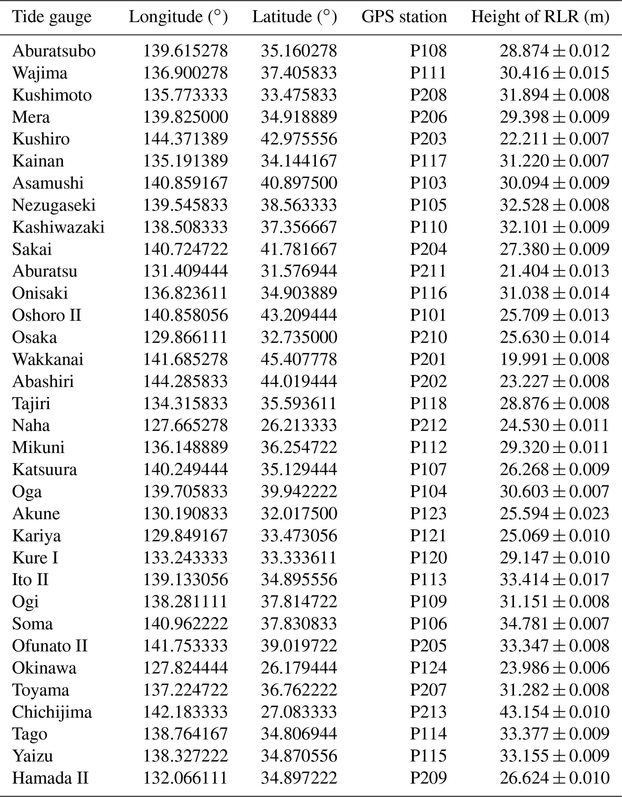
There are approximately 34 tide gauges around Japan listed on the PSMSL website, which have continuous annual data spanning from 1993 to 2019 and joint GPS data. The information on the 34 tide gauge stations and joint GPS stations around Japan is provided in the Appendix of this study. The data from GPS-leveled tide gauges around Japan were selected to validate the SDUST2020 MSS model.
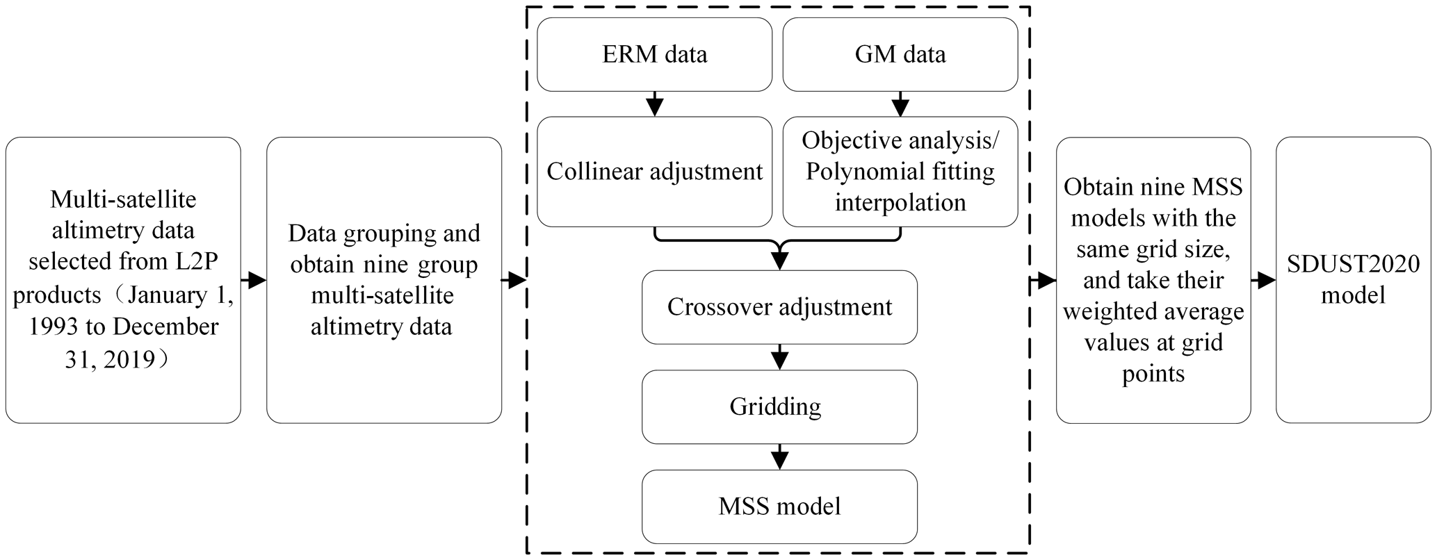
Figure 2 shows the data processing procedure used to establish the SDUST2020 model. First, the multi-satellite altimetry data (Table 1), spanning from 1 January 1993 to 31 December 2019 selected from L2P products, were grouped into 19-year-long moving windows shifted by 1 year, starting in January 1993, and nine groups of multi-satellite altimetry data were obtained. Second, the multi-satellite altimetry data of each group were independently processed to establish a global MSS model, including the collinear adjustment of ERM data, ocean variability correction of GM data (addressed by objective analysis and polynomial fitting interpolation), multi-satellite joint crossover adjustment, and the least-squares collocation (LSC) technique for gridding. Third, MSS models with a grid size of were established, resulting in nine MSS models with the same grid size. Finally, the SDUST2020 model was obtained by weighting the weighted average value of the nine models according to the reciprocal square of the estimated SSH error (derived from the LSC technique for gridding) at the same grid point. The calculation method is shown in Eqs. (1) and (2):
where msshi,SDUST2020 and erri,SDUST2020 are the SSH and the error of the SSH at the grid point i in the SDUST2020 model, respectively, and mssh and err are the SSH and the error of the SSH at the grid point i in each of the nine MSS models, respectively.
3.1 Ocean variability correction
The correction of altimeter data for ocean variability is a major challenge when attempting to establish an MSS model (Schaeffer et al., 2012; Pujol et al., 2018). Because the ground tracks of altimetry satellites with ERM coincide with each other, the ocean variability correction of ERM data can be solved using the collinear adjustment method. This method not only makes it possible to remove ocean variability (seasonal and interannual) but also to obtain the mean along-track SSH. The collinear adjustment method used in this study is the same as that described by Yuan et al. (2021).
Because GM data do not have the characteristics of repeated periods, such as ERM data, the ocean variability correction of GM data cannot be addressed by collinear adjustment. Fortunately, the ocean variability of GM data was obtained simultaneously using ERM data. For example, ERS-1/GM data contain the same ocean variability as the T/P data for the same period (1994–1995). Currently, the main methods for the correction of GM data for ocean variability are objective analysis or the use of polynomial functions (e.g., polynomial fitting interpolation, PFI). The objective analysis method is considered to be the best method to correct the ocean variability of GM data (Schaeffer et al., 2012; Pujol et al., 2018) and has been successfully applied to the establishment of MSS models, such as CLS11 and CLS15. It can be used to interpolate the ocean variability of one or more missions considered as a reference at the spatial and temporal positions of the satellite that would be corrected for ocean variability (Schaeffer et al., 2012). The objective analysis method used in this study is described by Yuan et al. (2021), and further details are provided by Le Traon et al. (1998, 2001, 2003) and Ducet et al. (2000).
T/P series (refer to T/P, Jason-1, Jason-2, and Jason-3) satellite altimetry data are widely known to have the highest measurement accuracy. Therefore, the mean along-track SSH of the continuous T/P series during 1993–2019 is used as the basis for calculating the ocean variability of the ERM data. The orbit inclination of T/P series satellites is approximately 66∘, whereas that of GM satellites is usually greater than 66∘. For example, the orbital inclinations of ERS-1/168, HY-2A/GM, SARAL/DP, and CryoSat-2 were 98.52, 99.3, 98.55, and 92∘, respectively. Therefore, the objective analysis method can only correct the ocean variability of GM data within the latitude range of 66∘ S to 66∘ N, whereas that beyond 66∘ S or 66∘ N cannot be corrected. In this study, when correcting GM data (such as ERS-1/168, HY-2A/GM, SARAL/DP, and CryoSat-2) for ocean variability, an objective analysis method was adopted for GM data between 66∘ S and 66∘ N, whereas the PFI method was adopted for GM data beyond 66∘ S or 66∘ N.
The basic principle of the PFI method can be expressed as follows: first, a fitting polynomial is used to fit the grid sea-level variation time series to extract the ocean variability, and the least squares solution is used to solve the fitting parameters; second, the ocean variability of GM data (above 66∘ S or 66∘ N) is interpolated with time as the independent variable to complete the ocean variability correction of GM data. The grid sea-level variation time series is the monthly averaged grid sea-level variation time series between 1993 and 2019 provided by AVISO, with a grid of . The fitting polynomial was as follows (Andersen and Knudsen, 2009; Jin et al., 2016):
where y is the sea-level variation time series, t is the time, k is the bias, B is the trend, C and D are the coefficients of the annual signal, and E and F are the coefficients of the semi-annual signal.
3.2 Crossover adjustment
The crossover adjustment is an important method for the data fusion of multi-satellite altimetry (Huang et al., 2008). The crossover adjustment method used in this study was performed in two steps: (i) condition adjustment at crossover adjustment and (ii) filtering and predicting the observational corrections along each track. This crossover adjustment method has been described in detail by Huang et al. (2008) and Yuan et al. (2020). In the crossover adjustment, an error model is established to reflect the combined effect of systematic errors (varied in very complicated ways) on the altimeter data. These errors include the radial orbit error, residual ocean variation, residual geophysical corrections, and so on. The error model can be expressed as follows (Huang et al., 2008; Yuan et al., 2020, 2021):
where f(t) is the systematic errors; t is the observation time of the SSH; a0, a1, bi, and are model parameters to be solved; ω represents the angular frequency corresponding to the duration of a surveying track (, where T0 and T1 represent the start and end times of the surveying track, respectively); and n is a positive integer determined by the length of the track. Based on empirical evidence, n is proposed to be 1–2 for a short track, 3–5 for a middle-long track, and 6–8 for a long track (Huang et al., 2008; Yuan et al., 2020).
Because the mean along-track SSH of the continuous T/P series derived from the collinear adjustment is used as the basis of the MSS model, it will remain unchanged and only correct crossover differences for other satellite altimetry data in the process of multi-satellite joint crossover adjustment. The details of the crossover adjustment method used in this study are discussed in Yuan et al. (2020, 2021).
3.3 Gridding
In this study, the LSC technique (Hwang, 1989; Rapp and Bašić, 1992) was used for gridding, which has been previously proven to be the most suitable method for gridding (Jin et al., 2016). In the process of gridding with the LSC, a second-order Markov process is used to describe the two-dimensional isotropic covariance function to obtain prior statistical information about the altimeter data and improve the accuracy of gridding. This process can be expressed as follows (Jordan, 1972; Moritz, 1978):
where d is the two-dimensional distance between the observation point and grid point; D0 is the local variance parameter, which can be expressed as the variance of all observed data participating in gridding within the local range; and α is the correlation length (where a 50 % correlation is obtained). Moreover, an accuracy of times the single-satellite crossover differences after the crossover adjustment was introduced into the LSC as the noise of the corresponding satellite data.
In the gridding process, the number of observation points within the range determined by the given search radius needs to be no less than 20, and the search radius is usually twice the grid spacing (e.g., 1′). When the number of observation points within a given search radius is less than 20, the search radius should be appropriately expanded until the conditions are met. The search method ensures at least five observation data points in each quadrant within the specified search range in the four quadrants centered on the grid point. The purpose of this method is to ensure that the observation data points around the grid point are uniformly distributed, which is conducive to ensuring the accuracy of grid data.
To improve the computational efficiency of gridding with the LSC, the globe was divided into several blocks, namely, blocks in the ranges of 80∘ S–60∘ N and 0–360∘, and 126 blocks in total. In the ranges of 60–80∘ N and 0–360∘, blocks were divided into 18 blocks. In this way, the globe was divided into 144 blocks, of which there are only 141 blocks that have SSH observations; two blocks (40–60∘ N, 60–100∘ W) in the Asian continent and one block (40–60∘ N, 240–260∘ W) in the American continent have no SSH observations. After gridding these 141 blocks, the number of the 141 grid SSH data is merged. When merging, the SSH of grid points on the repeated latitude and longitude lines was the SSH weighted average of grid points in the two adjacent blocks, and the weight was determined by the reciprocal of the square of the SSH error estimate at the grid points to obtain the final gridded global MSS model.
4.1 Processing results and analysis of altimetry data
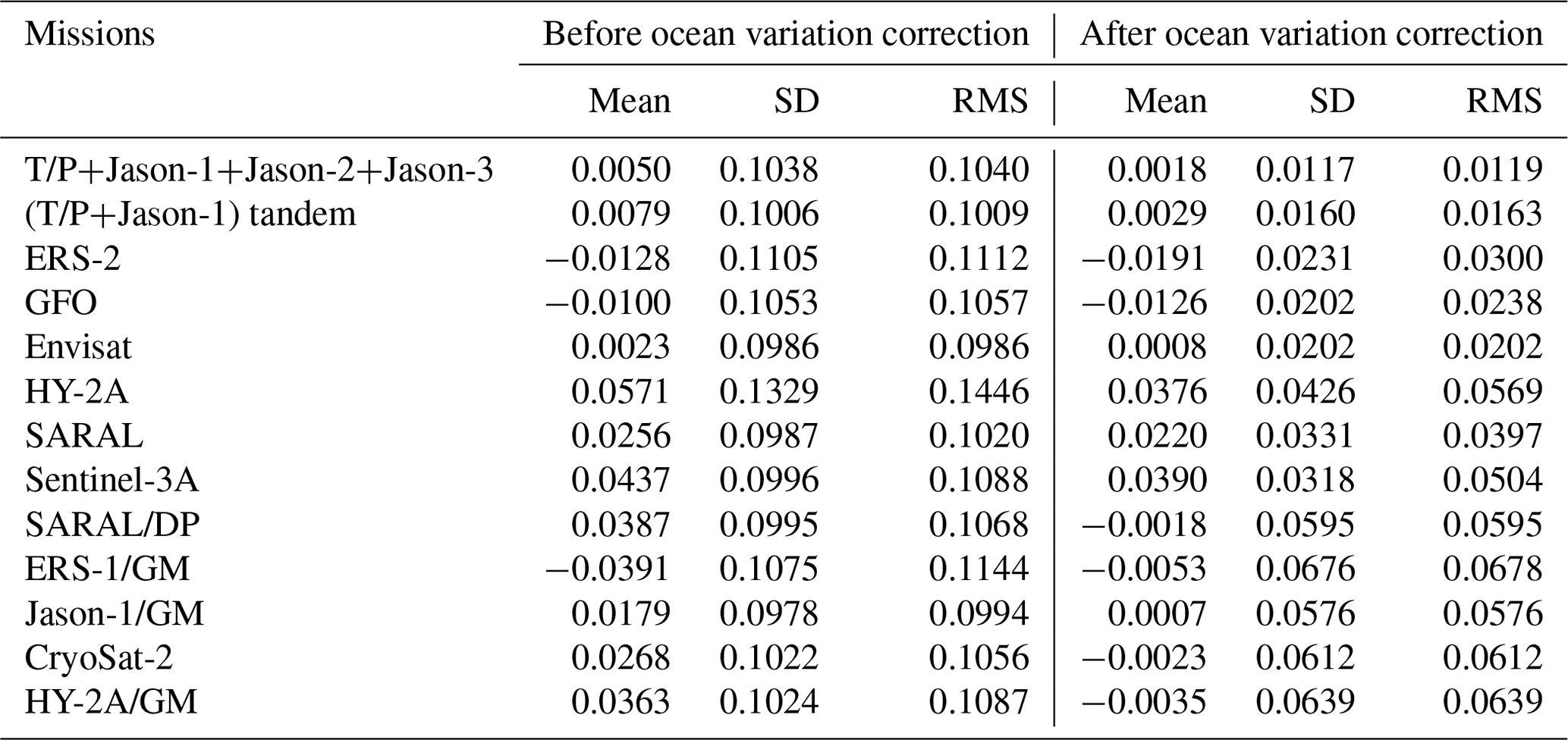
Ocean variability correction can eliminate or weaken the influence of sea-level long-wave ocean variation signals, partial satellite radial orbit errors, and residual errors after the correction of geophysical and environmental errors. Ocean variability correction was conducted for the altimeter missions in Table 1 in the global ocean, and the SSHs of these missions before and after ocean variability correction were compared with those of the SDUST2020 model. The statistical results of the comparisons are shown in Table 2, which show the impact of removing the ocean variability. As shown in Table 2, the magnitude of the RMS (between the SSH of each satellite altimetry mission and the SDUST2020 model) was reduced from decimeters before ocean variation correction to centimeters after ocean variation correction. The RMS of the T/P series (T/P+Jason-1+Jason-2+Jason-3) after ocean variation correction was the smallest (0.0119 m).
Table 2Statistical results of the comparison between heights of different altimeter missions and the SDUST2020 model before and after oceanic variability correction (unit: m).
Figures 3 and 4 show what could be achieved by correcting the ocean variability of Jason-1/GM. Figure 3 shows the differences between the SSHs of the Jason-1/GM and SDUST2020 model, where ocean variability has not been corrected. Before applying this correction, the differences in SSHs were dominant in the western boundary currents. However, these differences improved significantly after correction for ocean variability (Fig. 4).
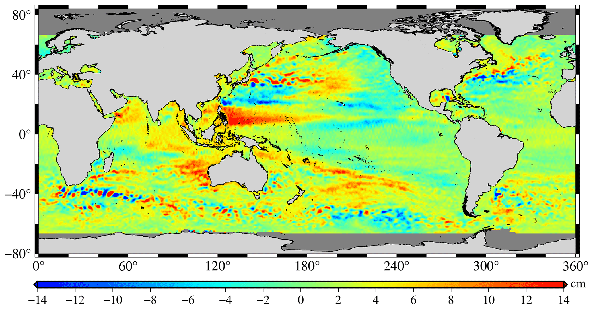
Figure 3Sea surface height differences between Jason-1/GM and the SDUST2020 model before oceanic variability correction.
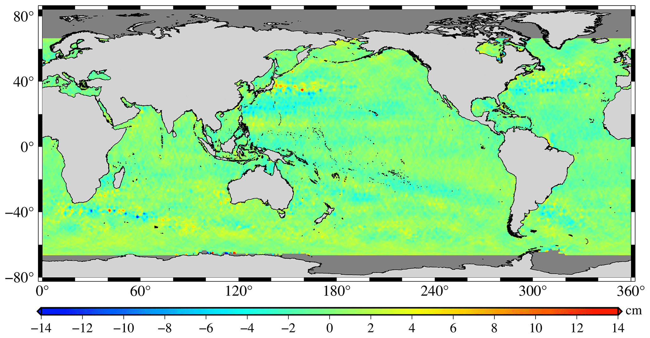
Figure 4Sea surface height differences between Jason-1/GM and the SDUST2020 model after oceanic variability correction.
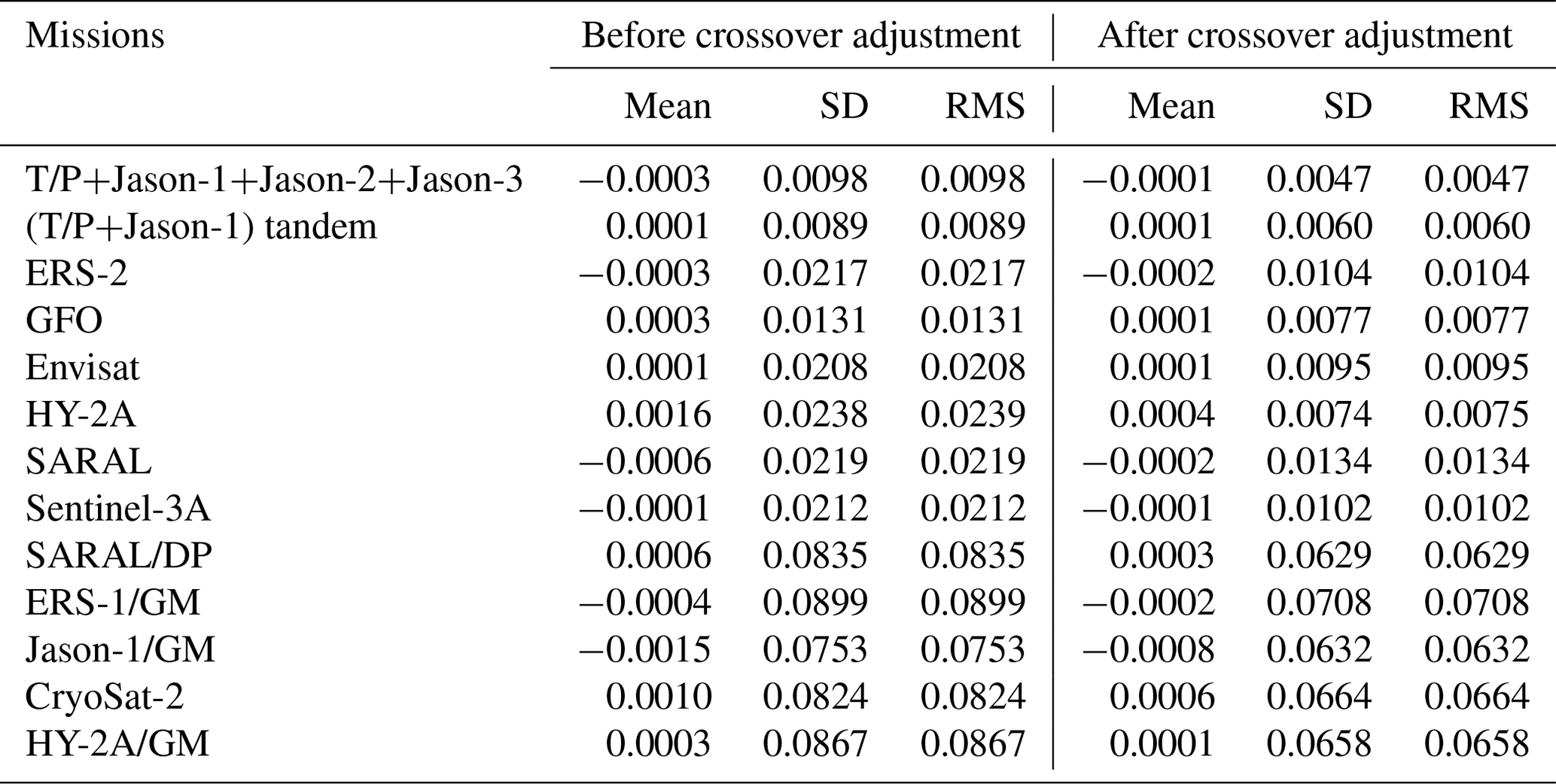
All of the altimeter missions listed in Table 1 were performed by self-crossover adjustment after completing the correction of ocean variability. Table 3 presents the statistical results of the crossover differences between these missions before and after the self-crossover adjustment. It can be seen from the results in Table 3 that the accuracy of all missions was greatly improved after self-crossover adjustment. The accuracy of the ERM data was improved by approximately 1 cm from 1–2 cm before adjustment to approximately 1 cm after adjustment, while that of the GM data was improved by approximately 2 cm from 7–9 to 6–7 cm. Moreover, the accuracy of the ERM data (average accuracy of approximately 1 cm) was much higher than that of the GM data (average accuracy of approximately 6 cm), and the accuracy of different missions was also different. Therefore, the accuracy of each mission is considered in the process of multi-satellite joint crossover adjustment and gridding with LSC.
Table 3Statistical results of crossover differences of different altimeter missions before and after self-crossover adjustment (unit: m).
4.2 Establishment of the SDUST2020 model
According to the procedure of data processing in Fig. 2, the SDUST2020 model was established using a 19-year moving average method from multi-satellite altimetry data (shown in Table 1). The SDUST2020 model is illustrated in Fig. 5, with a grid size of and a global coverage range of 80∘ S–84∘ N, with a reference time spanning from 1 January 1993 to 31 December 2019. As shown in Fig. 5, the global MSS was generally uneven, with the highest SSH of approximately 88 m and the lowest SSH of approximately −106 m, with a difference of 194 m.
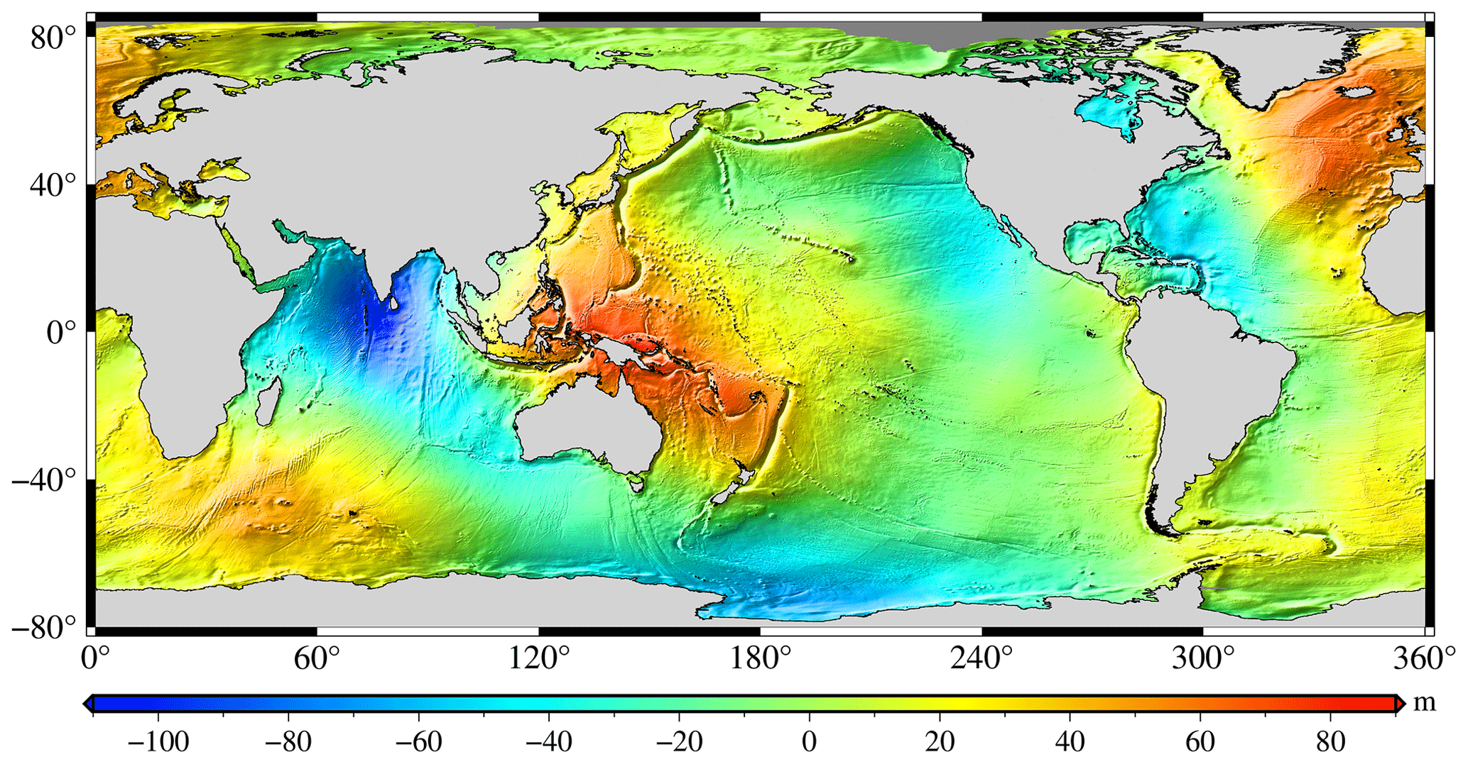
Figure 5Global mean sea surface model, SDUST2020.
Several independent methods have been proposed to validate the SDUST2020 model. First, we inspected the differences with other MSS models, such as CLS15 and DTU18; then, we compared the MSS models with the data of GPS-leveled tide gauges around Japan; and finally, we compared the independent altimeter data including ERM and GM data.
5.1 Comparison with CLS15 and DTU18 models
The CLS15 and DTU18 models are representative MSS models published by different institutions (CLS15 published by CLS and CNES and DTU18 published by DTU). In this study, these two models were used to validate the SDUST2020 model. Table 4 shows the information for the SDUST2020, CLS15, and DTU18 models. The main differences between SDUST2020, CLS15, and DTU18 are the reference period and altimeter data ingested. The reference period of SDUST2020 was 1993–2019, while that of CLS15 and DTU18 was 1993–2012. Compared to CLS15 and DTU18, SDUST2020 ingests more altimeter data. Among the altimeter data, Jason-3, HY-2A, and Sentinel-3A (ingested in the SDUST2020 model) were first used to establish an MSS model.
Table 4Mean sea surface models SDUST2020, CLS15, and DTU18.
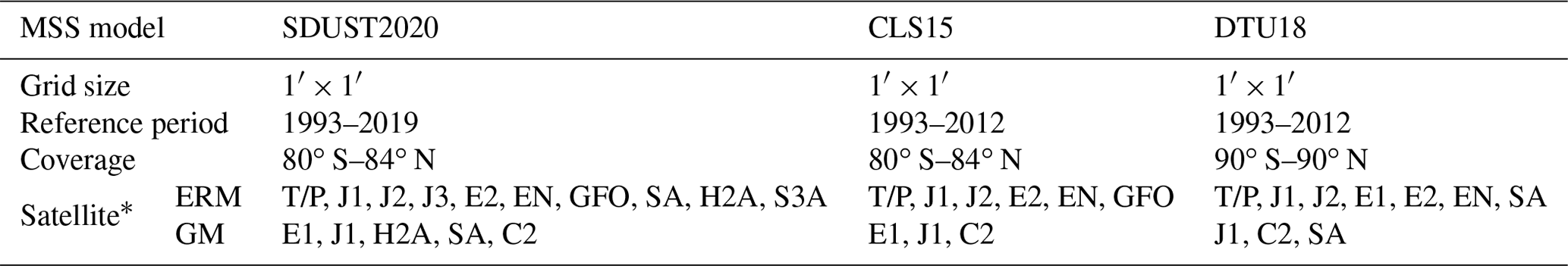
* T/P for TOPEX/Poseidon, J1 for Jason-1, J2 for Jason-2, J3 for Jason-3, E1 for ERS-1, E2 for ERS-2, EN for Envisat, H2A for HY-2A, C2 for CryoSat-2, S3A for Sentinel-3A, SA for SARAL.
Table 5 shows the comparative statistical results of the SDUST2020, CLS15, and DTU18 models in terms of SSH. In the comparison, the ocean variability caused by averaging over distinct periods (27 years from 1993 to 2019 for SDUST2020 and 20 years from 1993 to 2012 for CLS15 and DTU18) was removed, which was calculated from the monthly averaged grid sea-level variation time series between 1993 and 2019 provided by AVISO, with a grid of . Compared with DTU18, the SD of SDUST2020 was less than that of CLS15; compared with CLS15, the SD of SDUST2020 was also less than that of DTU18, while compared with SDUST2020, the SD of CLS15 was less than that of DTU18. Therefore, it can be inferred that the accuracy of these three models, from high to low, is SDUST2020, CLS15, and DTU18.
Table 5Statistical results of comparisons between different mean sea surface models (unit: m).
If the three models of SDUST2020, CLS15, and DTU18 are not correlated with each other, then according to the error propagation law, the SDs of these three models can be expressed as follows:
where SDS_C, SDS_D, and SDC_D are the SDs of SDUST2020 compared with CLS15, SDUST2020 compared with DTU18, and CLS15 compared with DTU18, respectively; SDS, SDC, and SDD are the SDs of SDUST2020, CLS15, and DTU18, respectively. According to the statistical results in Table 5, the SDs of SDUST2020, CLS15, and DTU18 can be calculated using Eq. (6), which are approximately 0.1318, 0.1613, and 0.2442 m, respectively. This result confirms that the accuracy of these three models, from high to low, is SDUST2020, CLS15, and DTU18.
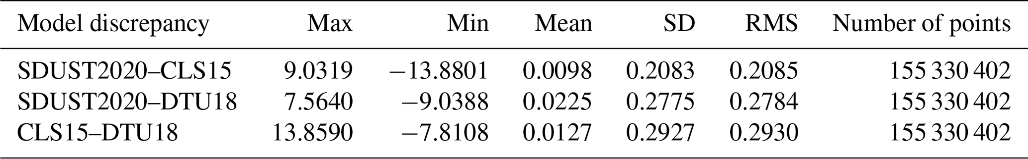
The results listed in Table 5 are the statistical results of the comparison between the three models in the global ocean. A total of 155 330 402 grid points are counted, including grid points in the coastal regions. After outliers in the differences are rejected by three times SD to avoid contamination by the poor observations around coastal regions, the results are shown in Table 6. It can be inferred that the differences between the three models are around 1–2 cm, and the SDUST2020 MSS and CLS15 MSS models have the best consistency.
Table 6Statistical results of comparisons between different mean sea surface models after rejecting outliers in differences by three times SD (unit: m).

The SSH differences between the SDUST2020, CLS15, and DTU18 models in the long and short wavelengths are shown in Fig. 6 (the SSH differences between SDUST2020 and CLS15), Fig. 7 (the SSH differences between SDUST2020 and DTU18), and Fig. 8 (the SSH differences between CLS15 and DTU18), which were drawn after Gaussian filtering with the tools available in the Generic Mapping Tools version 6.0 (GMT6.0) software (Wessel et al., 2019). Similar to Andersen et al. (2018), a wavelength of 150 km was selected as the dividing line between the long and short wavelengths. As shown in Figs. 6, 7, and 8, there were no significant differences between these models in the short wavelength (wavelength less than 150 km), and the average differences were within 2 cm, whereas there were some significant differences in the long wavelength (wavelengths greater than 150 km). The differences between these models at long wavelengths were mainly concentrated in the polar regions and the western boundary current region (including the Kuroshio Current, Gulf of Mexico, Agulhas Current, etc.). There are two reasons: on the one hand, it is related to the large sea level change in these regions (Jin et al., 2016); on the other hand, it is also related to the different altimeter data used and data processing methods implemented in the modeling (Andersen and Knudsen, 2009; Schaeffer et al., 2012; Pujol et al., 2018).
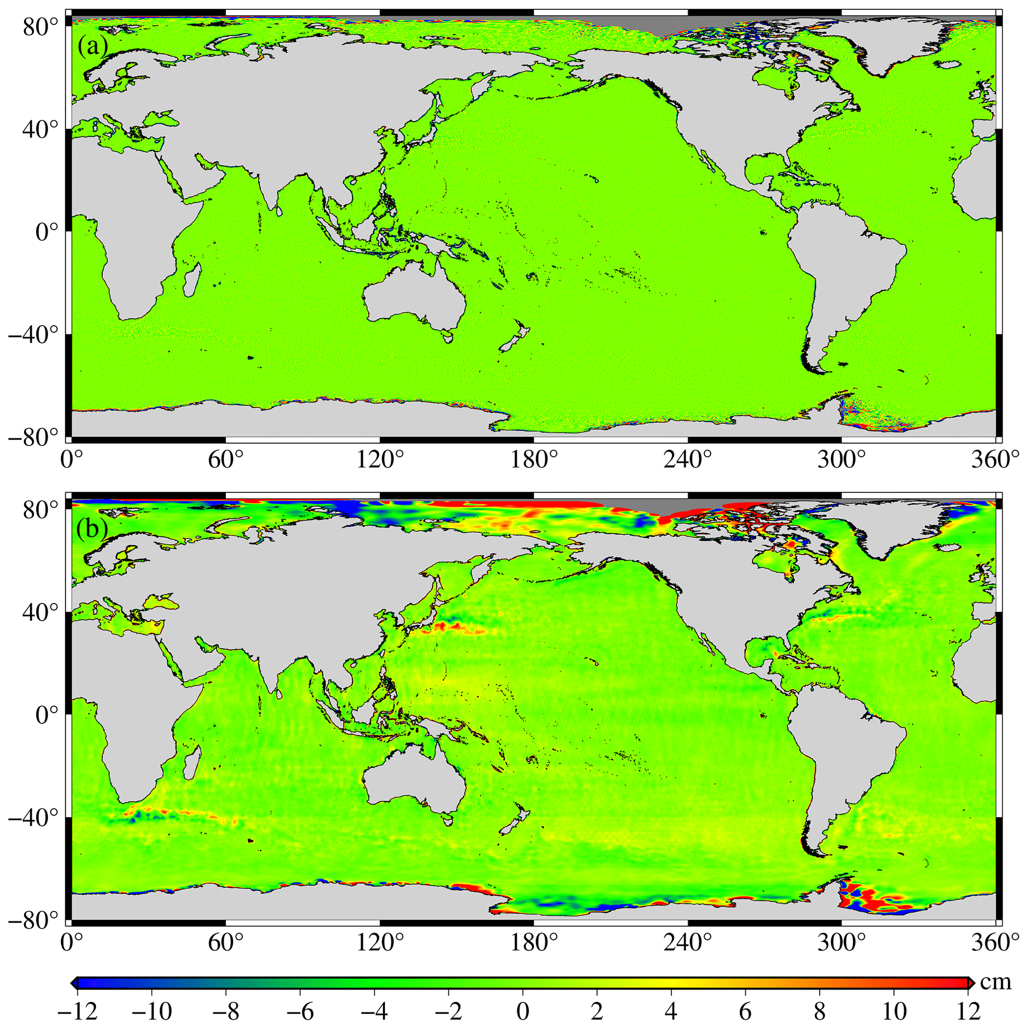
Figure 6Differences between SDUST2020 and CLS15: (a) wavelength less than 150 km and (b) wavelength greater than 150 km.
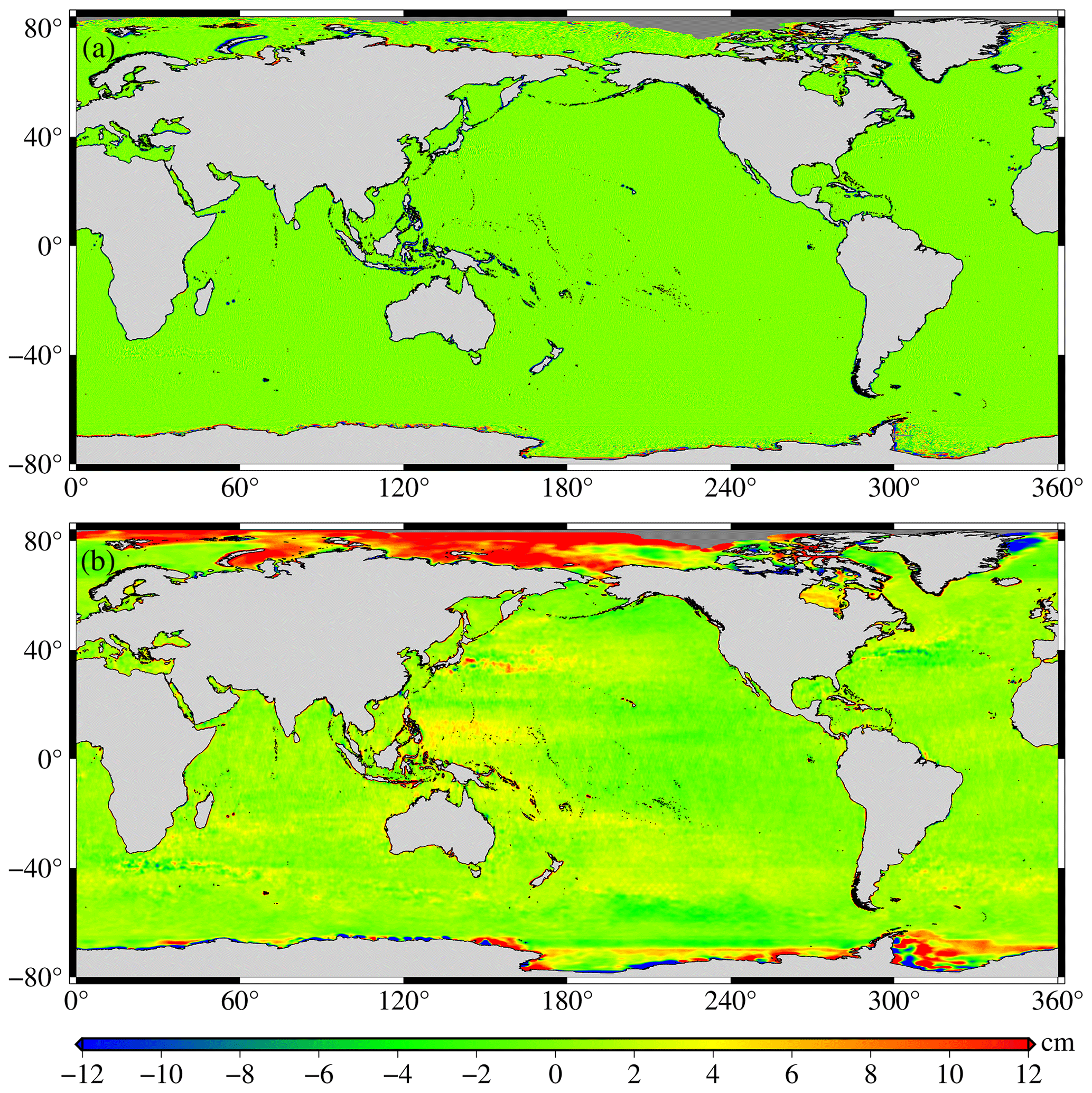
Figure 7Differences between SDUST2020 and DTU18: (a) wavelength less than 150 km and (b) wavelength greater than 150 km.
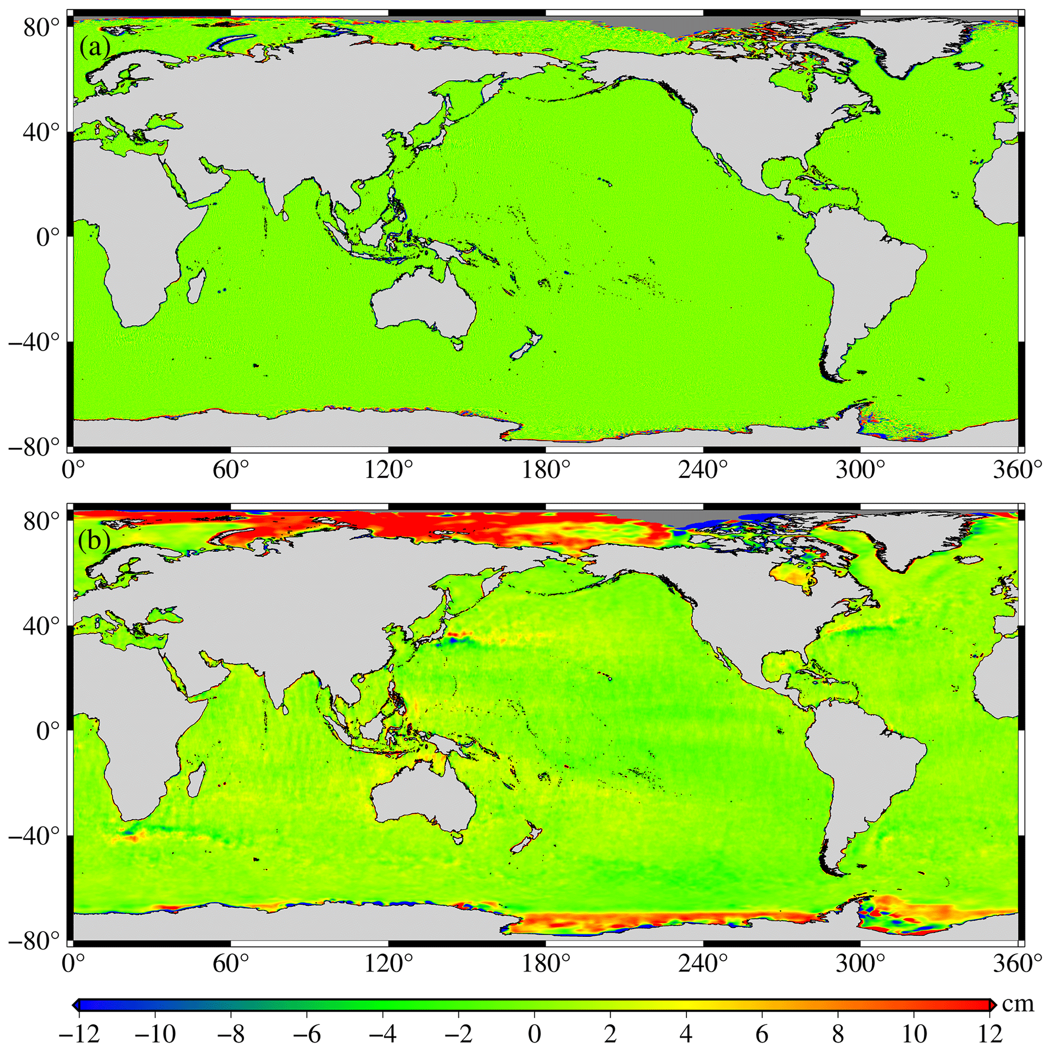
Figure 8Differences between CLS15 and DTU18: (a) wavelength less than 150 km and (b) wavelength greater than 150 km.
At the optimal interpolation (using the LSC technique for gridding) output, a calibrated formal error was obtained. The formal error is caused by three terms: an instrumental noise, a residual effect of the oceanic variability, and an along-track bias. These three terms are complementary and correspond, respectively, to white noise, a spatially correlated noise (at mesoscale wavelengths), and a long-wavelength error that is assumed to be constant along the tracks. The formal error does not match the precision of the MSS but is nonetheless an excellent indicator of the consistency of the grid (Schaeffer et al., 2012; Pujol et al., 2018).
Figures 9, 10, and 11 highlight the formal errors in SDUST2020, CLS15, and DTU18, respectively, which indicate that SDUST2020 was much more homogenous and accurate than CLS15 and DTU18. This is also confirmed by worldwide statistics. The average and RMS about the formal error of SDUST2020 were 1.0 and 1.5 cm, while those of CLS15 were 1.4 and 1.9 cm, and those of DTU18 were 1.9 and 2.0 cm.
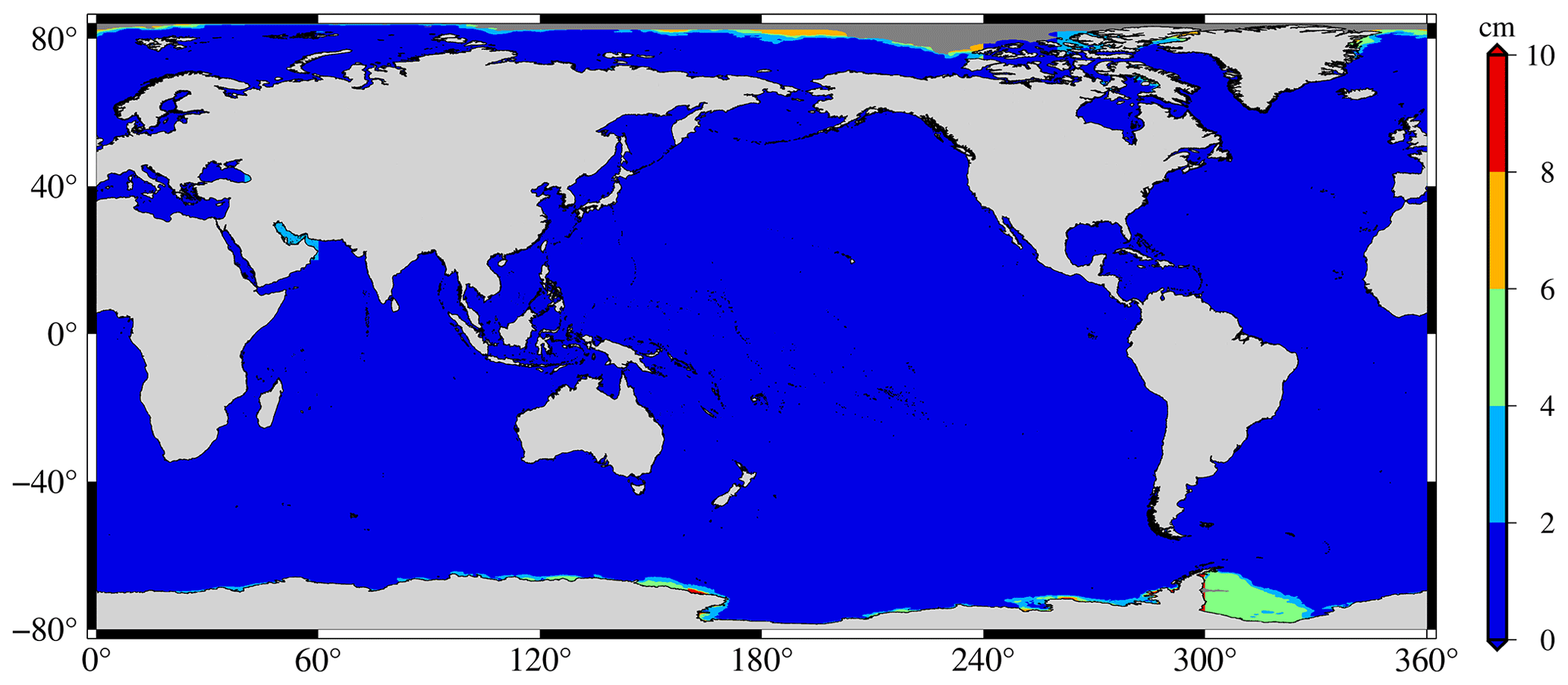
Figure 9Formal error of the SDUST2020 model.
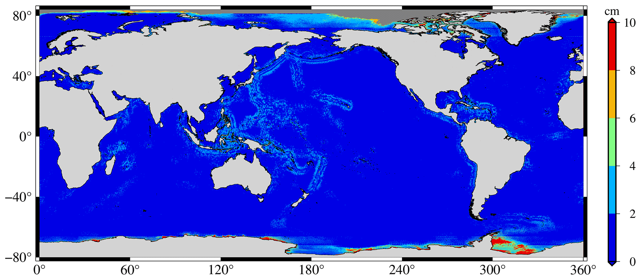
Figure 10Formal error of the CLS15 model.
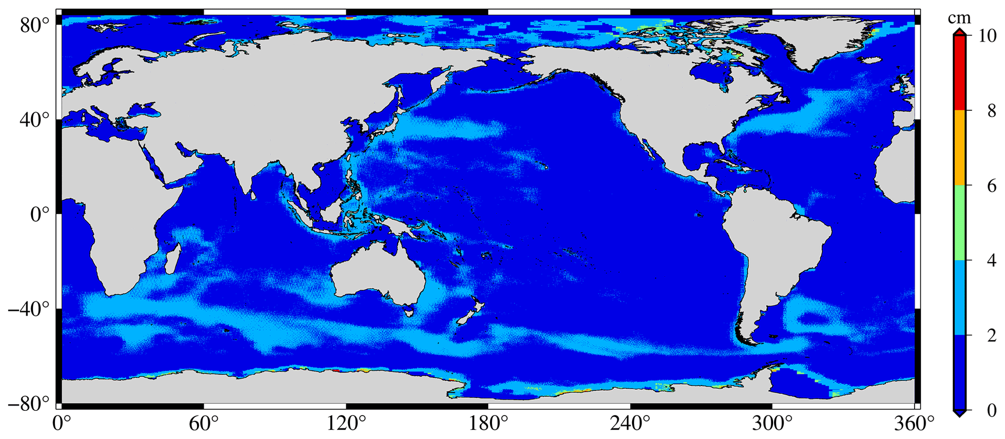
Figure 11Formal error of the DTU18 model.
5.2 Comparison with GPS-leveled tide gauges
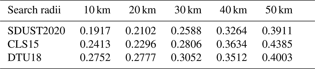
A comparison between 34 GPS-leveled tide gauges around Japan and the SSH of the SDUST2020, CLS15, and DTU18 models was used to independently validate the accuracy differences of the models that are close to the coast (Andersen and Knudsen, 2009). Before the comparison, the SSH obtained from the GPS-leveled tide gauges was adjusted to have the same reference ellipsoid as T/P. It is not clear how wide SSH can be represented by a single tide gauge. The SSH of different models at the location of the tide gauge was calculated by the reciprocal weighting of the spherical distance from the tide gauge to the points, which was determined by different search radii (e.g., 10, 20, 30, 40, and 50 km), which were centered on the tidal station. The SSH differences of different models compared with 34 GPS-leveled tide gauges around Japan with different search radii are shown in Fig. 12, and their SDs are listed in Table 7. As shown in Fig. 12 and Table 7, the larger the search radii, the greater the difference between the models and GPS-leveled tide gauges. In Table 7, the SD of the SSH differences between the MSS model and the GPS-leveled tide gauges reaches the decimeter level. The reason may be closely related to the poor observations of offshore altimeter data. The SD of the SSH differences of SDUST2020 compared with the GPS-level tide gauges is smaller than those of CLS15 and DTU18, indicating that the accuracy of SDUST2020 was better than that of CLS15 and DTU18.
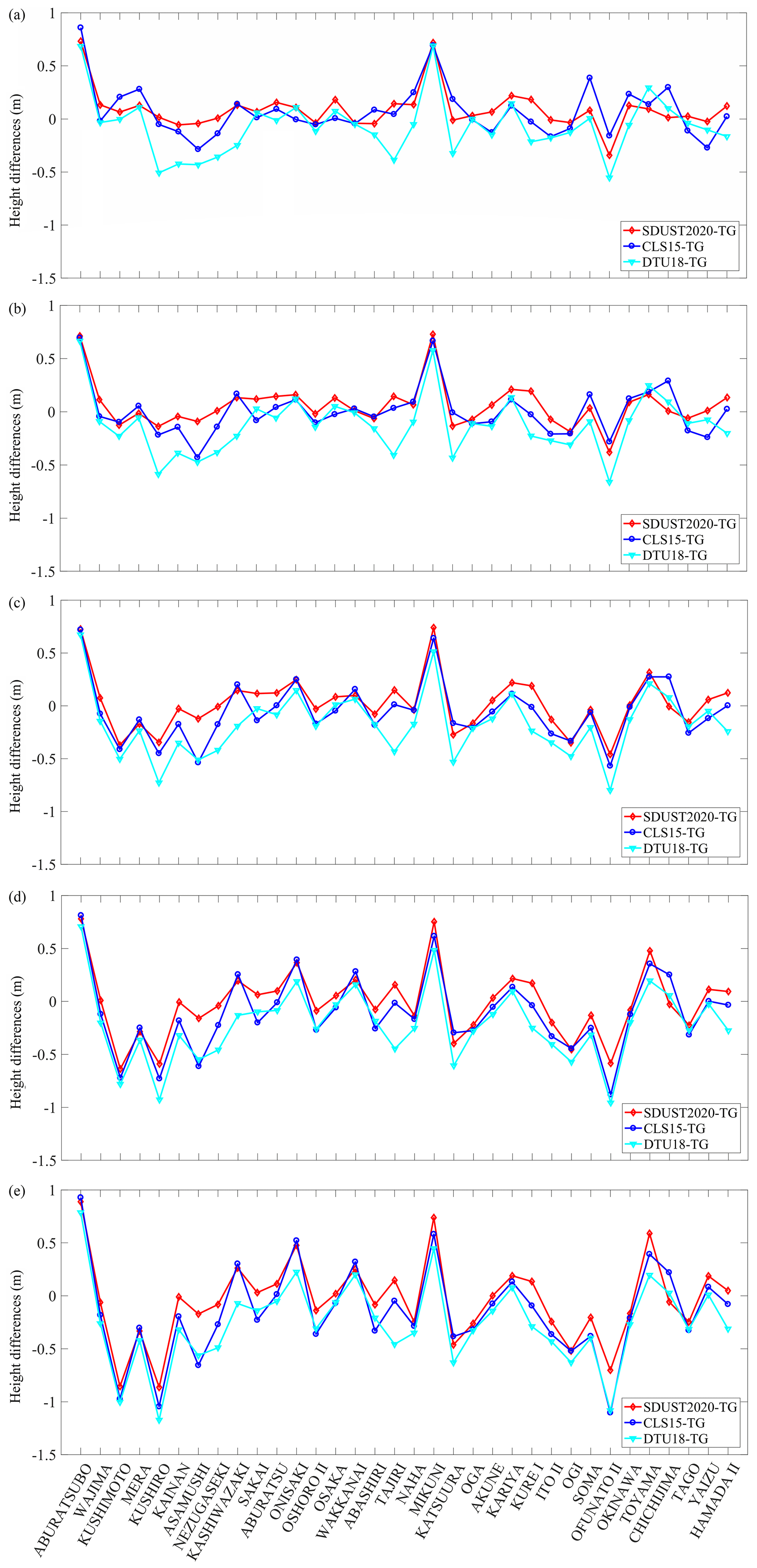
Figure 12Sea surface height differences of different models compared with 34 GPS-leveled tide gauges around Japan in different search radii. Panels (a), (b), (c), (d), and (e) correspond to the search radius of 10, 20, 30, 40, and 50 km, respectively.
Table 7SDs of SDUST2020, CLS15, and DTU18 models compared with GPS-leveled tide gauges around Japan in different search radii (unit: m).
5.3 Comparison with altimeter data
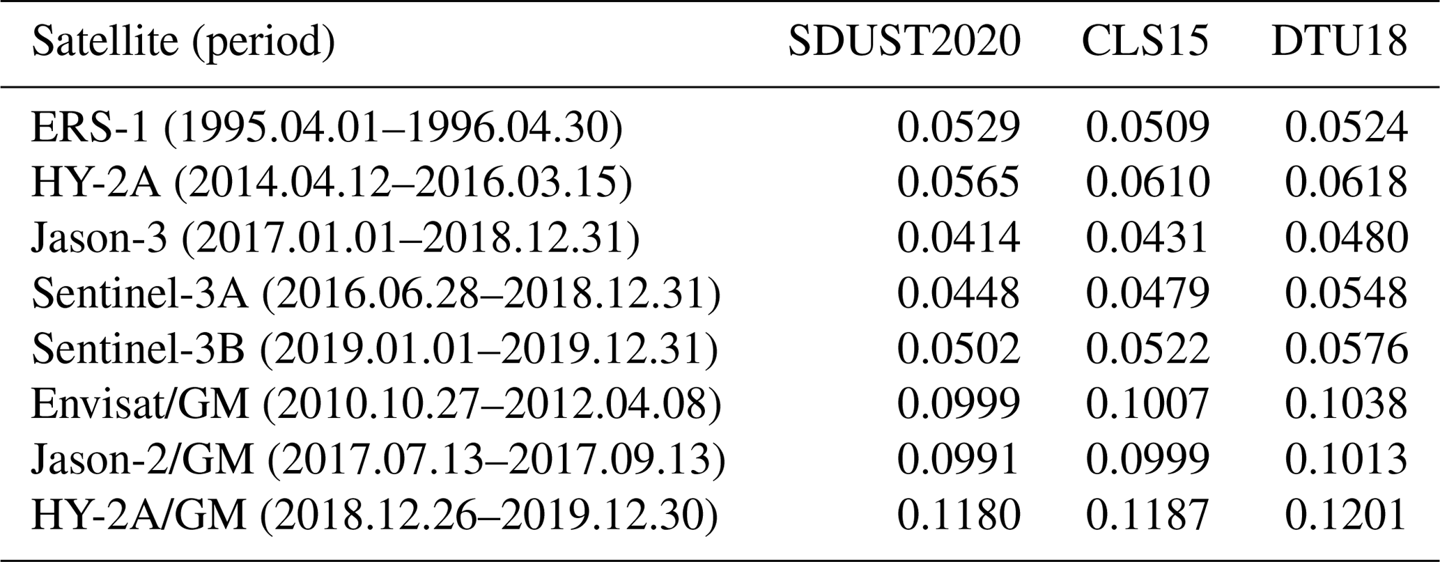
Comparison with the altimeter data can be used to estimate the accuracy of the MSS models (Andersen and Knudsen, 2009; Schaeffer et al., 2012; Jin et al., 2016), which is another effective way to validate MSS models. Several datasets were chosen, including the ERM and GM data. The ERM data were the mean along-track SSH after collinear adjustment, and the GM data were not processed by ocean variability correction. The ERM data included 1-year ERS-1, 2-year HY-2A, 2-year Jason-3, 2.5-year Sentinel-3A, and 1-year Sentinel-3B data, and the GM data included 1.5-year Envisat/GM, 2-month Jason-2/GM, and 1-year HY-2A/GM data. Among these, the data of Sentinel-3B and Envisat/GM were not ingested in the SDUST2020, CLS15, and DTU18 models, and the data of HY-2A, Jason-3, and Sentinel-3A were ingested in the SDUST2020 model, while they were not ingested in the CLS15 and DTU18 models.
Table 8 shows the differences in the SDs of the SSH for the SDUST2020, CLS15, and DTU18 models compared to the altimeter data. From the results in Table 8, the differences between the SDs given by these three models are at the millimeter level, but nearly all SDs given by SDUST2020 are lower than CLS15 and DTU18, indicative of higher accuracy. The SDs given by these three models were approximately 4–6 cm compared with the ERM data (the first five groups), approximately 10 cm compared with GM data (the last three groups), and almost half of the former. The reason may be that the altimeter data of the first five groups have been corrected for the ocean variability, while those of the last group have not.
Table 8SDs of the sea surface height differences of the models SDUST2020, CLS15, and DTU18 compared with satellite altimetry data (unit: m).
To more accurately assess and quantify the differences in the model errors for SDUST2020, CLS15, and DTU18 at different wavelengths, Sentinel-3B data (1 year, 2019.01.01–2019.12.31) were selected to calculate sea-level anomaly (SLA) along-track based on these three models and to obtain the SLA power spectral density (PSD). Because the Sentinel-3B data were independent of these three models, the difference between the SLA PSDs of Sentinel-3B along-track calculated based on these three models reflected the difference in the error of these three models (Pujol et al., 2018; Sun et al., 2021).
Figure 13a shows the mean global SLA PSD along Sentinel-3B tracks when different MSS models were used. As shown in Fig. 13a, all PSDs varied with the wavelength; the longer the wavelengths, the greater the PSDs, and there were also differences between the PSDs of different MSS models for different wavelengths. Since the SSH and MSS were based on independent data and periods, for long wavelengths (e.g., wavelengths longer than 150 km), the ocean variability signal dominated, for short wavelengths (e.g., wavelengths from ∼ 25 to 150 km), the errors of MSS models dominated, while for shorter wavelengths (e.g., wavelengths shorter than 25 km), the altimeter noise floor dominated (Pujol et al., 2018).
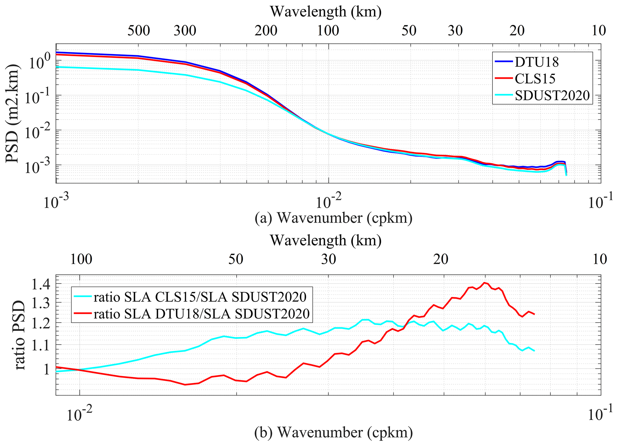
Figure 13(a) The SLA PSD along Sentinel-3B tracks using several models. (b) The ratio of SLA PSD from panel (a).
The PSD of the SDUST2020 model was significantly less than that of CLS15 and DTU18, and the PSD of CLS15 was slightly smaller than that of DTU18 for wavelengths longer than 150 km. The reason for the former was that the reference period of SDUST2020 (1993–2019) was longer than that of CLS15 and DTU18 (1993–2012), and the reason for the latter was that the data pre-processing method for Sentinel-3B is the same as that of the altimeter data ingested in the CLS15 model. This has also been confirmed by worldwide statistics. The average values of the SLA based on SDUST2020, CLS15, and DTU18 were 0.0155, 0.0494, and 0.0596 m, respectively, and the RMS values were 0.0525, 0.07919, and 0.0829 m, respectively.
Figure 13b shows the ratio between the PSD curves in Fig. 13a, which can better quantify the differences between the MSS models. Compared with the CLS15 model, the errors of the SDUST2020 model improved in the wavelength range from 25 to 150 km, with a maximal impact of approximately 40 km, which is an improvement of approximately 15 %.
Table 9SD of SLA for short wavelengths along the track of different altimeters, based on different MSS models (passband filtered from 25 to 150 km) (unit: m).
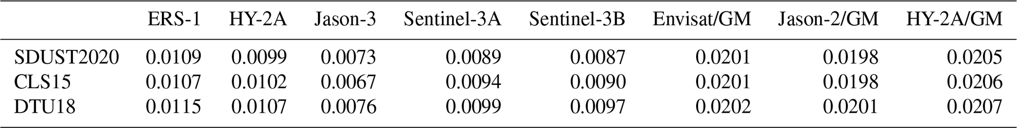
Table 9 lists the SD of the SLA of these three MSS models for wavelengths ranging from 25 to 150 km along different altimeter tracks. As shown in Table 9, the accuracy difference among these three models was very small, all at the sub-millimetre level; however, the accuracy of SDUST2020 was slightly better than those of CLS15 and DTU18.
The SDUST2020 MSS dataset is available open-access at https://doi.org/10.5281/zenodo.6555990 as an .nc file (Yuan et al., 2022). The dataset includes geospatial information (latitude and longitude) and mean sea surface height.
In this study, SDUST2020, a new global MSS model, was established using a 19-year moving average method from multi-satellite altimetry data. Its global coverage was from 80∘ S to 84∘ N with a grid size of and a reference period from January 1993 to December 2019.
Firstly, in comparison with the CLS15 and DTU18 models, the SDUST2020 model was innovative in the data processing method of model establishment, namely the 19-year moving average method; secondly, the reference period of the SDUST2020 model extended from 1993 to 2019, while CLS15 and DTU18 only ranged from 1993 to 2012; thirdly, the establishment of the SDUST2020 model integrated the altimeter data of HY-2A, Jason-3, and Sentinel-3A for the first time, which have not been used in the establishment of any other global MSS models.
Comparing SDUST2020 with the CLS15 and DTU18 models, the results presented in this study show that the accuracy of these three models, from high to low, is SDUST2020, CLS15, and DTU18. Comparing SDUST2020, CLS15, and DTU18 with the data of GPS-leveled tide gauges around Japan and the altimeter data of several satellites, these results show that the accuracy of SDUST2020 is better than that of CLS15 and DTU18.
Table A1Information of 34 tide gauge stations and joint GPS stations around Japan.
JY presented the algorithm and carried out the experimental results. JY and JGu prepared the paper and figures with contributions from all the co-authors. JGu, XL and JGa polished the entire manuscript. CZ and ZL downloaded altimeter products and other products in this work. All authors checked and gave related comments for this work.
The contact author has declared that none of the authors has any competing interests.
Publisher’s note: Copernicus Publications remains neutral with regard to jurisdictional claims in published maps and institutional affiliations.
We are very grateful to AVISO for providing the along-track Level-2+(L2P) products and the delayed-time gridded monthly mean of sea-level anomalies product, which can be obtained by freely downloading from AVISO's official website (ftp://ftp-access.aviso.altimetry.fr, last access: 5 January 2023). We are also thankful to CLS for providing the CNES_CLS15 MSS (ftp://ftp-access.aviso.altimetry.fr, last access: 5 January 2023) and DTU for providing the DTU18 MSS (https://ftp.space.dtu.dk/pub/, last access: 5 January 2023). The tide gauge records are available online (https://www.psmsl.org/, last access: 5 January 2023) and the GPS data are available online (https://www.sonel.org, last access: 5 January 2023).
This work was partially supported by the National Natural Science Foundation of China (grant nos. 42192535 and 41774001), the Autonomous and Controllable Project for Surveying and Mapping of China (grant no. 816517), the SDUST Research Fund (grant no. 2014TDJH101), and the Scientific Research Foundation for High-level Talents of Anhui University of Science and Technology (grant no. 2022yjrc66).
This paper was edited by François G. Schmitt and reviewed by Haihong Wang and two anonymous referees.
Andersen, O. B. and Knudsen, P.: DNSC08 mean sea surface and mean dynamic topography models, J. Geophys. Res.-Oceans, 114, 327–343, https://doi.org/10.1029/2008JC005179, 2009.
Andersen, O. B., Knudsen, P., and Bondo, T.: The mean sea surface DTU10 MSS-comparison with GPS and Tide Gauges, in: ESA Living Planet Symposium, Bergen, Norway, 28 June–2 July, 2010, https://articles.adsabs.harvard.edu/pdf/2010ESASP.686E.502A (last access: 5 January 2023), 2010.
Andersen, O. B., Knudsen, P., and Stenseng, L.: The DTU13 MSS (mean sea surface) and MDT (mean dynamic topography) from 20 years of satellite altimetry, in: IGFS 2014, International Association of Geodesy Symposia, edited by: Jin, S. and Barzaghi, R., 144, Springer, Cham, https://doi.org/10.1007/1345_2015_182, 2015.
Andersen, O. B., Piccioni, G., Stenseng, L., and Knudsen, P.: The DTU15 MSS (mean sea surface) and DTU15LAT (lowest astronomical tide) reference surface, in: Proceedings of the ESA Living Planet Symposium 2016, Prague, Czech Republik, 9–13 May 2016, https://ftp.space.dtu.dk/pub/DTU15/DOCUMENTS/MSS/DTU15MSS+LAT.pdf (last access: 5 January 2023), 2016.
Andersen, O. B., Knudsen, P., and Stenseng, L.: A new DTU18 MSS mean sea surface–improvement from SAR altimetry, in: 25 Years of Progress in Radar Altimetry Symposium, Portugal, 24–29 September, https://ftp.space.dtu.dk/pub/DTU18/MSS_MATERIAL/PRESENTATIONS/DTU18MSS-V2.pdf (last access: 5 January 2023), 2018.
Carrère, L., Lyard, F., Cancet, M., Guillot, A., and Dupuy, S.: FES 2014: a new global tidal model, OSTST Meeting, Lake Contance, Germany, http://meetings.aviso.altimetry.fr/fileadmin/user_upload/tx_ausyclsseminar/files/29Red1100-2_ppt_OSTST2014_FES2014_LC.pdf (last access: 5 January 2023), 2014.
CNES: Along-track level-2+ (L2P) SLA product handbook, SALPMU-P-EA-23150-CLS, Issue 2.0, https://www.aviso.altimetry.fr/fileadmin/documents/data/tools/hdbk_L2P_all_missions_except_S3.pdf (last access: 5 January 2023), 2020.
Ducet, N., Le Traon, P. Y., and Reverdin, G.: Global high-resolution mapping of ocean circulation from TOPEX/Poseidon and ERS-1 and -2, J. Geophys. Res.-Oceans, 105, 19477–19498, https://doi.org/10.1029/2000jc900063, 2000.
Guo, J., Hwang, C., and Deng, X.: Editorial: Application of satellite altimetry in marine geodesy and geophysics, Front. Environ. Sci., 10, 910562, https://doi.org/10.3389/feart.2022.910562, 2022.
Holgate, S. J., Matthews, A., Woodworth, P. L., Rickards, L. J., Tamisiea, M. E., Bradshaw, E., Foden, P. R., Gordon, K. M., Jevrejeva, S., and Pugh, J.: New Data Systems and Products at the Permanent Service for Mean Sea Level, J. Coastal Res., 29, 493–504, https://doi.org/10.2112/JCOASTRES-D-12-00175.1, 2013.
Huang, M., Zhai, G., Ouyang, Y., Lu, X., Liu, C., and Wang, R.: Integrated data processing for multi-satellite missions and recovery of marine gravity field, Terr. Atmos. Ocean. Sci., 19, 103–109, https://doi.org/10.3319/TAO.2008.19.1-2.103(SA), 2008.
Hwang, C. W.: High precision gravity anomaly and sea surface height estimation from Geos-3/Seasat altimeter data, M.S. Thesis. Dept. of Geodetic Science and Surveying, The Ohio State University, Columbus, OH, USA, 1989.
Jin, T., Li, J., and Jiang, W.: The global mean sea surface model WHU2013, Geod. Geodyn., 7, 202–209, https://doi.org/10.1016/j.geog.2016.04.006, 2016.
Jordan, S. K.: Self-consistent statistical models for the gravity anomaly, vertical deflections, and undulation of the geoid, J. Geophys. Res., 77, 3660–3670, https://doi.org/10.1029/JB077i020p03660, 1972.
Le Traon, P. Y., Nadal, F., and Ducet, N.: An improved mapping method of multisatellite altimeter data, J. Atmos. Ocean. Tech., 15, 522–534, https://doi.org/10.1175/1520-0426(1998)015<0522:AIMMOM>2.0.CO;2, 1998.
Le Traon, P. Y., Dibarboure, G., and Ducet, N.: Use of a high-resolution model to analyze the mapping capabilities of multiple-altimeter missions, J. Atmos. Ocean. Tech., 18, 1277–1288, https://doi.org/10.1175/1520-0426(2001)018<1277:UOAHRM>2.0.CO;2, 2001.
Le Traon, P. Y., Faugère, Y., Hernandez, F., Dorandeu, J., Mertz, F., and Ablain, M.: Can we merge GEOSAT follow-on with TOPEX/Poseidon and ERS-2 for an improved description of the ocean circulation?, J. Atmos. Ocean. Tech., 20, 889–895, https://doi.org/10.1175/1520-0426(2003)020<0889:CWMGFW>2.0.CO;2, 2003.
Moritz, H.: Least-squares collocation, Rev. Geophys., 16, 421–430, https://doi.org/10.1029/RG016i003p00421, 1978.
Pujol, M.-I., Schaeffer, P., Faugère, Y., Raynal, M., Dibarboure, G., and Picot, N.: Gauging the improvement of recent mean sea surface models: a new approach for identifying and quantifying their errors, J. Geophys. Res.-Oceans, 123, 5889–5911, https://doi.org/10.1029/2017JC013503, 2018.
Rapp, R. H. and Bašić, T.: Oceanwide gravity anomalies from GEOS-3, Seasat and Geosat altimeter data, Geophys. Res. Lett., 19, 1979–1982, https://doi.org/10.1029/92GL02247, 1992.
Santamaria-Gomez, A., Gravelle, M., Dangendorf, S., Marcos, M., Spada, G., and Wöppelmann, G.: Uncertainty of the 20th century sea-level rise due to vertical land motion errors, Earth. Planet. Sc. Lett., 473, 24–32, https://doi.org/10.1016/j.epsl.2017.05.038, 2017.
Schaeffer, P., Faugére, Y., Legeais, J. F., Ollivier, A., Guinle, T., and Picot, N.: The CNES_CLS11 global mean sea surface computed from 16 Years of satellite altimeter data, Mar. Geod., 35, 3–19, https://doi.org/10.1080/01490419.2012.718231, 2012.
Sun, W., Zhou, X., Yang, L., Zhou, D., and Li, F.: Construction of the mean sea surface model combined HY-2A with DTU18 MSS in the antarctic ocean, Front. Environ. Sci., 9, 697111, https://doi.org/10.3389/fenvs.2021.697111, 2021.
Wessel, P., Luis, J. F., Uieda, L., Scharroo, R., Wobbe, F., Smith, W. H. F., and Tian, D.: The generic mapping tools version 6, Geochem. Geophy. Geosy., 20, 5556–5564, https://doi.org/10.1029/2019GC008515, 2019.
Yuan, J., Guo, J., Liu, X., Zhu, C., Niu, Y., Li, Z., Ji, B., and Ouyang, Y.: Mean sea surface model over China seas and its adjacent ocean established with the 19-year moving average method from multi-satellite altimeter data, Cont. Shelf Res., 192, 104009, https://doi.org/10.1016/j.csr.2019.104009, 2020.
Yuan, J., Guo, J., Zhu, C., Hwang, C., Yu, D., Sun, M., and Mu, D.: High-resolution sea level change around China seas revealed through multi-satellite altimeter data, Int. J. Appl. Earth Obs., 102, 102433, https://doi.org/10.1016/j.jag.2021.102433, 2021.
Yuan, J., Guo, J., Zhu, C., Li, Z., Liu, X., and Gao, J.: SDUST2020 MSS: A global mean sea surface model determined from multi-satellite altimetry data, Zenodo [data set], https://doi.org/10.5281/zenodo.6555990, 2022.