The consolidated European synthesis of CH₄ and N₂O emissions for the European Union and United Kingdom: 1990–2019

Knowledge of the spatial distribution of the fluxes of greenhouse gases (GHGs) and their temporal variability as well as flux attribution to natural and anthropogenic processes is essential to monitoring the progress in mitigating anthropogenic emissions under the Paris Agreement and to inform its global stocktake. This study provides a consolidated synthesis of CH₄ and N₂O emissions using bottom-up (BU) and top-down (TD) approaches for the European Union and UK (EU27 + UK) and updates earlier syntheses (Petrescu et al., 2020, 2021). The work integrates updated emission inventory data, process-based model results, data-driven sector model results and inverse modeling estimates, and it extends the previous period of 1990–2017 to 2019. BU and TD products are compared with European national greenhouse gas inventories (NGHGIs) reported by parties under the United Nations Framework Convention on Climate Change (UNFCCC) in 2021. Uncertainties in NGHGIs, as reported to the UNFCCC by the EU and its member states, are also included in the synthesis. Variations in estimates produced with other methods, such as atmospheric inversion models (TD) or spatially disaggregated inventory datasets (BU), arise from diverse sources including within-model uncertainty related to parameterization as well as structural differences between models. By comparing NGHGIs with other approaches, the activities included are a key source of bias between estimates, e.g., anthropogenic and natural fluxes, which in atmospheric inversions are sensitive to the prior geospatial distribution of emissions. For CH₄ emissions, over the updated 2015–2019 period, which covers a sufficiently robust number of overlapping estimates, and most importantly the NGHGIs, the anthropogenic BU approaches are directly comparable, accounting for mean emissions of 20.5 Tg CH₄ yr⁻¹ (EDGARv6.0, last year 2018) and 18.4 Tg CH₄ yr⁻¹ (GAINS, last year 2015), close to the NGHGI estimates of 17.5±2.1 Tg CH₄ yr⁻¹. TD inversion estimates give higher emission estimates, as they also detect natural emissions. Over the same period, high-resolution regional TD inversions report a mean emission of 34 Tg CH₄ yr⁻¹. Coarser-resolution global-scale TD inversions result in emission estimates of 23 and 24 Tg CH₄ yr⁻¹ inferred from GOSAT and surface (SURF) network atmospheric measurements, respectively. The magnitude of natural peatland and mineral soil emissions from the JSBACH–HIMMELI model, natural rivers, lake and reservoir emissions, geological sources, and biomass burning together could account for the gap between NGHGI and inversions and account for 8 Tg CH₄ yr⁻¹. For N₂O emissions, over the 2015–2019 period, both BU products (EDGARv6.0 and GAINS) report a mean value of anthropogenic emissions of 0.9 Tg N₂O yr⁻¹, close to the NGHGI data (0.8±55 % Tg N₂O yr⁻¹). Over the same period, the mean of TD global and regional inversions was 1.4 Tg N₂O yr⁻¹ (excluding TOMCAT, which reported no data). The TD and BU comparison method defined in this study can be operationalized for future annual updates for the calculation of CH₄ and N₂O budgets at the national and EU27 + UK scales. Future comparability will be enhanced with further steps involving analysis at finer temporal resolutions and estimation of emissions over intra-annual timescales, which is of great importance for CH₄ and N₂O, and may help identify sector contributions to divergence between prior and posterior estimates at the annual and/or inter-annual scale. Even if currently comparison between CH₄ and N₂O inversion estimates and NGHGIs is highly uncertain because of the large spread in the inversion results, TD inversions inferred from atmospheric observations represent the most independent data against which inventory totals can be compared. With anticipated improvements in atmospheric modeling and observations, as well as modeling of natural fluxes, TD inversions may arguably emerge as the most powerful tool for verifying emission inventories for CH₄, N₂O and other GHGs. The referenced datasets related to figures are visualized at https://doi.org/10.5281/zenodo.7553800 (Petrescu et al., 2023).

1 Introduction

Atmospheric concentrations of greenhouse gases (GHGs) reflect a balance between emissions from sources and removals by sinks, with the former arising from both human activities and natural sources and the latter being found in the biosphere, oceans and atmospheric oxidation. Increasing levels of GHGs in the atmosphere due to human activities have been the major driver of climate change since the pre-industrial period (pre-1750). In 2020, GHG mole fractions were at record highs, with globally averaged mole fractions reaching 1889±2 ppb (parts per billion) for methane (CH₄) and 333.2±0.1 ppb for nitrous oxide (N₂O), representing 262 % and 123 % of the respective pre-industrial levels (WMO, 2021). Since 2004, when CH₄ registered a negative dip, the trend in the CH₄ concentration in the atmosphere has continued to increase (NOAA, 2020, atmospheric data: https://www.esrl.noaa.gov/gmd/ccgg/trends_ch4/, last access: May 2022). This increase was attributed to anthropogenic emissions from agriculture – livestock enteric fermentation and rice cultivation (12 %) and fossil-fuel-related activities (17 %), combined with a contribution from natural tropical wetlands (Saunois et al., 2020; Thompson et al., 2018; Feng et al., 2022a, b). The increase in atmospheric N₂O also continues to rise with the highest annual increase ever recorded in 2020 (https://gml.noaa.gov/ccgg/trends_n2o/, last access: May 2022). The main sources remain linked to agriculture, particularly the application of nitrogen fertilizers and livestock manure on agricultural land (FAO, 2020, 2015; IPCC, 2019; Tian et al., 2020).

National GHG emission inventories (NGHGIs) are prepared and reported on an annual basis by Annex I parties¹ to the United Nations Framework Convention on Climate Change (UNFCCC). These inventories contain annual time series of each country's GHG emissions from the 1990 base year² until 2 years before the year of reporting and were originally set to track progress towards their reduction targets under the Kyoto Protocol (UNFCCC, 1997). Non-Annex I parties³ to the UNFCCC also provide emission estimates in biennial update reports (BURs) as well as through national communications (NCs); however, non-Annex I emissions are not reported annually and do not use harmonized formats due to the comparatively less stringent reporting requirements. Annex I NGHGIs are reported according to the Decision 24/CP.19 of the UNFCCC Conference of the Parties (COP), which states that the national inventories shall be compiled using the methodologies provided in the 2006 IPCC Guidelines for National Greenhouse Gas Inventories (2006). The 2006 IPCC guidelines provide methodological guidance for estimating emissions for well-defined sectors using national activity and available emission factors. Decision trees indicate the appropriate level of methodological sophistication (methodological tier) based on the absolute contribution of the sector to the national GHG balance (whether the source or sink is a key category or not) and the country's national circumstances (availability and resolution of national activity data and emission factors). Generally, Tier 1 methods are based on global or regional default emission factors that can be used with aggregated activity data, while Tier 2 methods rely on country-specific factors and/or activity data at a higher subsector resolution. Tier 3 methods are based on more detailed process-level modeling or even facility-level emission measurements. Annex I parties are furthermore required to estimate and report uncertainties in emissions (95 % confidence interval) following the 2006 IPCC guidelines using, as a minimum requirement, the Gaussian error propagation method (approach 1). Annex I parties may use Monte Carlo methods (approach 2) or a hybrid approach and are encouraged to do so.

Annex I NGHGIs should follow principles of transparency, accuracy, consistency, completeness and comparability (TACCC) under the guidance of the UNFCCC (UNFCCC, 2014), and as mentioned above, they shall be completed following the 2006 IPCC guidelines (IPCC, 2006). In addition, the 2019 Refinement to the 2006 IPCC Guidelines for National Greenhouse Gas Inventories (IPCC, 2019), which may be used to complement the 2006 IPCC guidelines, has updated sectors with additional emission sources and provides guidance on the use of atmospheric data for independent verification of GHG inventories. Complementary to the NGHGIs, research groups and international institutions produce estimates of national GHG emissions, with two kind of approaches: atmospheric inversions (top-down, TD) and GHG inventories based on the same principle as NGHGI but using activity and/or emissions factors from (partially) different sources (bottom-up, BU).

The two approaches (BU and TD) provide useful insights on emissions from two different point of view. First, TD approaches act as an additional quality control tool for BU and NGHGI approaches and facilitate a deeper understanding of the processes driving changes in different elements of GHG budgets. Second, NGHGIs cover regularly only a subset of countries (Annex I), and it is therefore necessary to construct BU estimates independently for all countries. Furthermore, while additional BU methods do not have prescribed standards like the IPCC guidelines, independent BU methods can draw on different input data or can provide estimates at higher sectoral resolution and therefore add complementary information to help quality control NGHGIs and help inform climate mitigation policy processes. Additionally, BU estimates are needed as input for TD estimates. As there is no formal guideline to estimate uncertainties in TD or BU approaches, uncertainties are usually assessed from the spread of different estimates within the same approach, though some groups or institutions report uncertainties for their individual estimates using a variety of methods, for instance, by performing sensitivity tests (Monte Carlo approach) on input data parameters. However, this can be logistically and computationally difficult when dealing with complex process-based models.

Despite the important insights gained from complementary BU and TD emission estimates, it should be noted that comparisons with the official reported is not always straightforward. BU estimates often share common methodology and input data, and, through harmonization, structural differences between BU estimates and NGHGIs can be bridged. However, the use of common input data, albeit to varying extents, restricts the independence between the datasets and, from a verification perspective, may limit the conclusions drawn from the comparisons. On the other hand, TD estimates are constrained by independent atmospheric observations and can serve as an additional, almost fully independent quality control for NGHGIs. Nonetheless, structural differences between NGHGIs (what sources and sinks are included and where and when emissions/removals occur) and the actual fluxes of GHGs to the atmosphere must be factored in to the comparison of estimates. While NGHGIs go through a central quality assurance and quality control (QA/QC) review process, the IPCC procedures do not incorporate mandatory large-scale observation-derived verification. Nevertheless, the individual countries may use atmospheric data and inverse modeling within their data quality control, quality assurance and verification processes, with expanded and updated guidance provided in chapter 6 of the 2019 refinement to the 2006 IPCC guidelines (IPCC, 2019). So far, only a few countries (e.g., Switzerland, the UK, New Zealand and Australia) have used atmospheric observations to constrain national emissions and documented these verification activities in their National Inventory Reports (Bergamaschi et al., 2018a).

A key priority in the current policy process is to facilitate the 5-yearly global stocktakes (GSTs) of the Paris Agreement, the first of which is in 2023, and to assess collective progress towards achieving the near- and long-term objectives, considering mitigation, adaptation and means of implementation. The GSTs are expected to create political momentum for enhancing commitments in nationally determined contributions (NDCs) under the Paris Agreement. Though the modalities of the GSTs implementation are not clear, the key component of this process will be the NGHGI reporting by countries under the enhanced transparency framework of the Paris Agreement. Under the framework, emission reporting will move away from the differential Annex I and non-Annex I reporting requirements and become more harmonized across parties. Non-Annex I parties will be required to follow the 2006 IPCC guidelines and provide regular (biennial) national GHG inventory reports to the UNFCCC, alongside developed countries, which will continue to submit their inventories on an annual basis. Some developing countries will face challenges to construct and subsequently update their NGHGIs and meet the more-stringent reporting requirements.

The work presented in this paper covers dozens of distinct datasets and models, in addition to the individual country submissions to the UNFCCC of the EU member states and the UK. As Annex I parties, the NGHGIs of the EU member states and the UK are consistent with the general guidance laid out in IPCC (2006) yet still differ in specific approaches, models and parameters, in addition to differences underlying activity datasets. A comprehensive investigation of detailed differences between all datasets is beyond the scope of this paper, though systematic analyses have been previously made for specific sectors (e.g., agriculture; Petrescu et al., 2020) and by the Global Carbon Project CH₄ and N₂O syntheses (Saunois et al., 2020; Tian et al., 2020). The focus of this paper is on updates of the information from Petrescu et al. (2021), discussing whenever needed the changes in terms of emissions and trends. The data from Petrescu et al. (2021) are labeled as v2019, while the latest results are labeled as v2021. Except for one on N₂O, the global inversions did not provide an update for v2021, and, therefore, the earlier results are incorporated into this synthesis.

As Petrescu et al. (2021) is the most comprehensive comparison of the NGHGI and research datasets (including both TD and BU approaches) for the EU27 + UK to date, the focus of the current paper is on improvement of estimates in the most recent version in comparison with the previous one, including changes in the uncertainty estimates and identification of the knowledge gaps and added value for policy making. Such exercises of yearly updates are needed to improve the different respective approaches and furthermore can inform the development of formal verification systems. Official NGHGI emissions are compared with research datasets, including necessary harmonization of the latter on total emissions to ensure consistency. Differences and inconsistencies between emission estimates were analyzed, and recommendations were made towards future evaluation of NGHGI data. It is important to remember that uncertainties provided by the NGHGIs are intended to be used in prioritization and decision-making (vol. 1, chap. 3, IPCC, 2006) and not to enable comparisons between countries or other datasets. In addition, individual spatially disaggregated research emission datasets often lack quantification of uncertainty. Here, the focus is on the median and minimum/maximum (min/max) range of different research products of the same type to get a first estimate of uncertainty (see Sect. 2). For those datasets providing uncertainties, new uncertainty reduction maps are presented (see Sect. 3.1.5). For those models/inventories that did not provide an update for this study, the previously published time series are shown.

2 CH₄ and N₂O data sources and estimation approaches

The CH₄ and N₂O emissions in the EU27 + UK from inversions and anthropogenic emission inventories from various BU approaches covering specific sectors were analyzed. The data (Table 2) span the period from 1990 to 2019, with some of the data only available for shorter time periods or up until 2020. The estimates are available both from peer-reviewed literature and from unpublished research results from the VERIFY project (Table 1 and Appendix A), and in this work they are compared with NGHGIs reported in 2021 (time series for 1990–2019). Data sources are summarized in Table 2 with the detailed description of all products provided in Appendix A1–A3.

For both CH₄ and N₂O BU approaches, inventories of anthropogenic emissions covering all sectors (EDGARv6.0 and GAINS) and models and inventories limited to agriculture (CAPRI, FAOSTAT, DayCent, ECOSSE) were used. For CH₄ biogeochemical models of natural peatland emissions (JSBACH–HIMMELI) and lake and reservoir emissions (Lauerwald et al., 2019; Thompson et al., 2022), as well as updated data for inland waters (rivers, lakes and reservoirs in preparation for the RECCAP2 project, Appendix A2.1) and updated data for total geological emissions (Etiope et al., 2019), were used. Emissions from gas hydrates and termites are not included as they are close to zero in the EU27 + UK (Saunois et al., 2020). Anthropogenic NGHGI CH₄ emissions from the land use, land use change and forestry (LULUCF) sector are very small for the EU27 + UK (3 % in 2019 including biomass burning) (Sect. 2.2).

TD approaches include both regional and global inversions, with the latter having a coarser spatial resolution. These estimates are described in Sect. 2.3.

For N₂O emissions, the same global BU inventories as for CH₄, natural emissions from inland waters (rivers, lakes and reservoirs, RECCAP2, Appendix A3.1) were used, which did not change with respect to Petrescu et al. (2021). In this study, about 66 % of the N₂O emitted by Europe's natural rivers is considered anthropogenic indirect emissions, caused by leaching and runoff of N fertilizers from the agriculture sector. One important update is the inclusion of estimates of natural N₂O emissions from soils simulated with the O-CN model (Zaehle et al., 2011). These emissions are derived from model simulations in which land use and atmospheric CO₂ remain constant, but climate varies through to 2020. These estimates are considered to be closer to what background natural N₂O emissions would be in the present day, so they were used for subtraction from outputs of inversions (as it has a reasonable representation of the inter-annual variability, IAV). The TD N₂O inversions include one regional inversion FLEXINVERT and three global inversions (Friedlingstein et al., 2019; Tian et al., 2020; Patra et al., 2022). Agricultural sector emissions of N₂O were presented in detail by Petrescu et al. (2020). In this current study, CAPRI and ECOSSE models and FAO provided updated emissions, with the latter additionally covering non-CO₂ emissions from biomass burning as a contribution to LULUCF. Fossil-fuel-related emissions and industrial emissions were obtained from GAINS (see Appendix A1). Table A2 in Appendix A presents the methodological differences of the current study with respect to Petrescu et al. (2020, 2021).

Table 1 Sectors included in this study and data sources (bold) providing estimates for these sectors.

^a For consistency with the NGHGI, here we refer to the five reporting sectors as defined by the UNFCCC and the Paris Agreement decision (18/CMP.1), the IPCC guidelines (IPCC, 2006), and their refinement (IPCC, 2019), with the only exception being that the latest IPCC refinement groups together agriculture and LULUCF sectors in one sector (agriculture, forestry and other land use – AFOLU).
^b The term “natural” refers here to unmanaged natural CH₄ emissions (peatlands, mineral soils, geological, inland waters and biomass burning) not reported under the UNFCCC LULUCF sector.
^c Anthropogenic (managed) agricultural soils can also have a level of natural emissions.
^d Natural soils (unmanaged) can have both natural and anthropogenic emissions.

The units used in this paper are metric tonnes (t) (1 kt = 10⁹ g; 1 Mt = 10¹² g) of CH₄ and N₂O. The referenced data used for the figures' replicability purposes are available for download at https://doi.org/10.5281/zenodo.7553800 (Petrescu et al., 2023). Upon request, the codes necessary to plot the figures in the same style and layout can be provided. The focus is on EU27 + UK emissions. In the VERIFY project, an additional web tool was developed which allows for the selection and display of all plots shown in this paper (as well as the companion paper on CO₂), not only for the EU member states and UK but for a total of 79 countries and groups of countries in Europe (Table A1, Appendix A). The data, located on the VERIFY project website (http://webportals.ipsl.jussieu.fr/VERIFY/FactSheets/, last access: January 2023), are free and can be accessed upon registration.

2.1 CH₄ and N₂O anthropogenic emissions from NGHGI

Anthropogenic CH₄ emissions from the four UNFCCC sectors (excluding LULUCF) were grouped together. Anthropogenic CH₄ emissions in 2019 account for 17.1 Tg CH₄ yr⁻¹ and represent 10.5 % of the total EU27 + UK emissions (in CO₂ eq., GWP 100 years, IPCC AR4⁴). CH₄ emissions are predominantly related to agriculture (9.2±0.8 Tg CH₄ yr⁻¹ or 53.8 % in 2019 (52.5 % in 2018) of the total EU27 + UK CH₄ emissions). Anthropogenic NGHGI CH₄ emissions from the LULUCF sector are very small for the EU27 + UK, e.g., 0.5 Tg CH₄ yr⁻¹ or 3 % in 2019, including emissions from biomass burning.

Regarding CH₄ emissions from wetlands, following the recommendations of the 2013 IPCC wetlands supplement (IPCC, 2014) only emissions from managed wetlands are reported by parties. According to NGHGI data between 2008 and 2018, managed wetlands in the EU27 + UK for which emissions were reported under LULUCF (common reporting format, CRF, Table 4(II) accessible for each EU27 + UK country; https://unfccc.int/process-and-meetings/transparency-and-reporting/reporting-and-review-under-the-convention/greenhouse-gas-inventories-annex-i-parties/national-inventory-submissions-2019, last access: December 2022) represent one-fourth of the total wetland area in the EU27 + UK (Giacomo Grassi, EC-JRC, personal communication), and their emissions summed up in 2019 to 0.1 Tg CH₄ yr⁻¹.

Anthropogenic N₂O emissions (excluding LULUCF) in 2019 account for 0.8 Tg N₂O yr⁻¹ and represent 6.2 % of the total EU27 + UK emissions in CO₂ eq. N₂O emissions are predominantly related to agriculture (0.6 Tg N₂O yr⁻¹ or 73.0 % in 2019 (73.5 % in 2018) of the total EU27 + UK (including LULUCF + biomass burning) N₂O emissions) but are also found in the other sectors (Tian et al., 2020). In addition, N₂O has natural sources, which are defined as the pre-industrial background emissions before the use of synthetic N fertilizers and intensive agriculture and derive from natural processes in soils but also in lakes, rivers and reservoirs (Maavara et al., 2019; Lauerwald et al., 2019; Tian et al., 2020).

2.2 CH₄ and N₂O anthropogenic and natural emissions from other bottom-up estimates

Data from five global datasets and models of CH₄ and N₂O anthropogenic emission inventories were used, namely CAPRI, DayCent, ECOSSE, FAOSTAT, GAINS and EDGARv6.0 (Table 3). These estimates are not completely independent from NGHGIs (see Fig. 4 in Petrescu et al., 2020) as they integrate their own sectorial modeling with the UNFCCC data (e.g., common activity data and IPCC emission factors) when no other source of information is available. The CH₄ biomass and biofuel burning emissions are included in NGHGI under the UNFCCC LULUCF sector, although they are identified as a separate category by the Global Carbon Project CH₄ budget synthesis (Saunois et al., 2020). For both CH₄ and N₂O, CAPRI (Britz and Witzke, 2014; Weiss and Leip, 2012) and FAOSTAT (FAO, 2022) report only agricultural emissions. DayCent and ECOSSE report only emissions for agriculture N₂O. Out of all BU inventories, only CAPRI reported new uncertainties for 2014, 2016 and 2018, while values for EDGARv6.0 were the same (Solazzo et al., 2021) as those reported in Petrescu et al. (2021).

In this study, natural CH₄ emissions are included under the category “peatlands” and “other natural emissions”, with the latter including geological emissions, biomass burning emissions and two estimates of inland waters (rivers, lakes and reservoirs). One inland water estimate comes from process-based models and is based on the Rosentreter et al. (2021) with ranges from Bastviken et al. (2011) and Stanley et al. (2016), and the second represents an upscaled estimate for inland waters from the RECCAP2 project.

For peatlands and mineral soils, the JSBACH–HIMMELI framework was used. Additionally, the ensemble of 13 monthly gridded estimates of peatland emissions based on different land surface models as calculated for Saunois et al. (2020) was used as described in Appendix B2. Geological emissions were initially based on the global gridded emissions from Etiope et al. (2019) and previously estimated to be 1.3 Tg CH₄ yr⁻¹ (Petrescu et al., 2021). For this study these emissions were recalculated, using more detailed input data related to the activity, i.e., a more precise estimate of the continental oil–gas-field area (which determines the potential area of microseepage) and offshore seepage area (Appendix A2), and now account for 3.3 Tg CH₄ yr⁻¹ (0.9 Tg CH₄ yr⁻¹ from offshore marine seepage and 2.4 Tg CH₄ yr⁻¹ onshore). This rescaled geological source represents the second largest natural component accounting for 42 % of the total EU27 + UK natural CH₄ emissions. The upscaled inland waters (rivers, lakes and reservoirs) are the largest component of natural emissions (3.3 Tg CH₄ yr⁻¹ and ranging from 2.7 to 4.3 Tg CH₄ yr⁻¹) and account for 44 %. The remaining 14 % of emissions are attributed to peatlands, mineral soils and biomass burning. Overall, in the EU27 + UK the natural emissions thus accounted for 8 Tg CH₄ yr⁻¹. Finally, It should be noted that, to a small extent, the CH₄ natural emissions from waters are also due to an anthropogenic component, namely eutrophication following N fertilizer leaching to inland waters. Globally, the contribution of eutrophication is estimated to lead to a further increase in lake and reservoir emission by 30 % to 90 % over the 21st century, which would be the result of a ∼3-times-higher nutrient loading to lakes and reservoirs (Beaulieu et al., 2019), similar to the review by Li et al. (2021), who gathered a lot of proof that eutrophication significantly increased CH₄ emissions. In temperate Europe, eutrophication contributes significantly to the overall increase in natural emissions, and Rinta et al. (2017) found that eutrophic, central European lakes show CH₄ emission rates which are about 1 order of magnitude higher than those of oligotrophic boreal lakes, and this study's model results are consistent with it.

The N₂O anthropogenic emissions from inventory datasets belong predominantly to agriculture and are associated with two main categories: (1) direct emissions from the agricultural sector where synthetic fertilizers and manure were applied, as well as from manure management, and (2) indirect emissions on non-agricultural land and water receiving anthropogenic N through atmospheric N deposition, leaching and runoff (also from agricultural land). Additional anthropogenic emissions result from industrial processes, in particular, adipic and nitric acid production, which are declining owing to the implementation of emission abatement technologies. Other N₂O emissions come from the wastewater treatment activities and fossil fuel combustion.

In this study, “natural” N₂O fluxes refer to emissions from inland waters (lakes, rivers and reservoirs, Maavara et al., 2019; Lauerwald et al., 2019, and references in Appendix C) which include also lakes with dams. The other component is the natural N₂O emissions from soils simulated with the O-CN model (Zaehle et al., 2011). Regarding the inland water emissions, more than half of the emissions (56 % globally, Tian et al., 2020, and 66 % for Europe this study) are due to enhanced N inputs from fertilizers, manure, sewage and, to a smaller extent, atmospheric N deposition. However, emissions from natural soils in this study are considered anthropogenic because, according to the country-specific National Inventory Reports (NIRs), all land in the EU27 + UK is considered to be managed.

For both CH₄ and N₂O the natural biomass burning emissions from GFEDv4.1 (van der Werf et al., 2017) are included in Figs. 1, 4b, 5b, 9 and 13, while for CH₄ only, biomass burning emissions from the GCP 2020 (Saunois et al., 2020) are included in Fig. 6.

2.3 CH₄ and N₂O emission data from inversions

Atmospheric inversions optimize prior estimates of emissions and sinks through modeling frameworks that utilize atmospheric observations as a constraint on fluxes. Emission estimates from inversions depend on the dataset of atmospheric measurements and the choice of the atmospheric model, as well as on other inputs (e.g., prior emissions and their uncertainties). Inversion results were taken from original publications without evaluation of their performance through specific metrics; e.g., fit to independent cross-validation atmospheric measurements (Bergamaschi et al., 2013, 2018; Patra et al., 2016). Some of the inversions allow for explicit attribution to different sectors, while others optimize all fluxes in each grid cell and then attribute emissions to sectors using prior grid cell fractions (see details in Saunois et al., 2020, for global inversions).

For CH₄, the same set of 9 regional inversions and 22 global inversions as listed in Table 3 and presented in Petrescu et al. (2021) was used. While many different inversions exist, it should be stressed that the variants are not completely independent of one another. Table B4 in Appendix B in Petrescu et al. (2021) illustrates this by documenting to what extent the transport models, priors and atmospheric measurement data vary between the inversion datasets. The subset of InGOS inversions (Bergamaschi et al., 2018b) belongs to a project where all models used the same atmospheric data over Europe covering the period of 2006–2012. The global inversions from Saunois et al. (2020) were not updated for this work and cover a period until 2017.

The regional inversions generally use both higher-resolution prior data and higher-resolution transport models, and, e.g., TM5-JRC runs simultaneously over the global domain at coarse resolution and over the European domain at higher resolution, with atmospheric CH₄ concentration boundary conditions taken from global fields. For CH₄, 11 global inversions use GOSAT for the period of 2010–2017, 8 global inversions use surface stations (SURF) from 2000 to 2017, and two global models use SURF from 2010–2017 and one global model uses SURF from 2003–2017 (see Table 4 in Saunois et al., 2020). All regional inversions use observations from SURF stations as a base of their emission calculation.

Table 2 Data sources for CH₄ and N₂O emissions used in this study.

For N₂O, one regional inversion (FLEXINVERT) for the 2005–2019 period and three global inversions for the period of 1998–2016 from Tian et al. (2020) and Thompson et al. (2019) were used as listed in Table 3. These estimates were not updated for this paper. These inversions are not completely independent from each other since most of them use the same input information (Appendix B3). The regional inversion uses a higher-resolution atmospheric transport model for Europe, with atmospheric N₂O concentration boundary conditions taken from global model fields. As all inversions produced total rather than anthropogenic emissions, emissions from soils (O-CN) and inland waters (lakes, rivers and reservoirs) were subtracted from the total emissions. Note that inland water emissions include anthropogenic emissions from N-fertilizer leaching, accounting for 66 % of the inland water emissions in the EU27 + UK. In 2019, emissions from inland waters represented 1.4 % of the total UNFCCC NGHGI (2021) N₂O emissions.

The largest share of N₂O emissions comes from agricultural soils (direct and indirect emissions from the applications of fertilizers, whether synthetic or manure) contributing in 2019 79 % of the total N₂O emissions (excluding LULUCF) in the EU27 + UK. In Petrescu et al. (2021), Table B1.3 in Appendix B1 presented the allocation of emissions by activity type covering all agricultural activities and natural emissions, following the IPCC (2006) sector classification scheme. Each data product has its own particular way of grouping emissions and does not necessarily cover all emission activities. The main inconsistencies between process-based models and inventories are observed regarding activity allocation in the two models, ECOSSE and DayCent. ECOSSE only estimates direct N₂O emissions and does not estimate downstream emissions of N₂O, for example, indirect emissions from nitrate leached into water courses, which also contributes to an underestimation of total N₂O emissions. Field burning emissions are also not included by most of the data sources.

3 Results and discussion

3.1 Comparing CH₄ emission estimates from different approaches

3.1.1 Estimates of European and regional total CH₄ fluxes

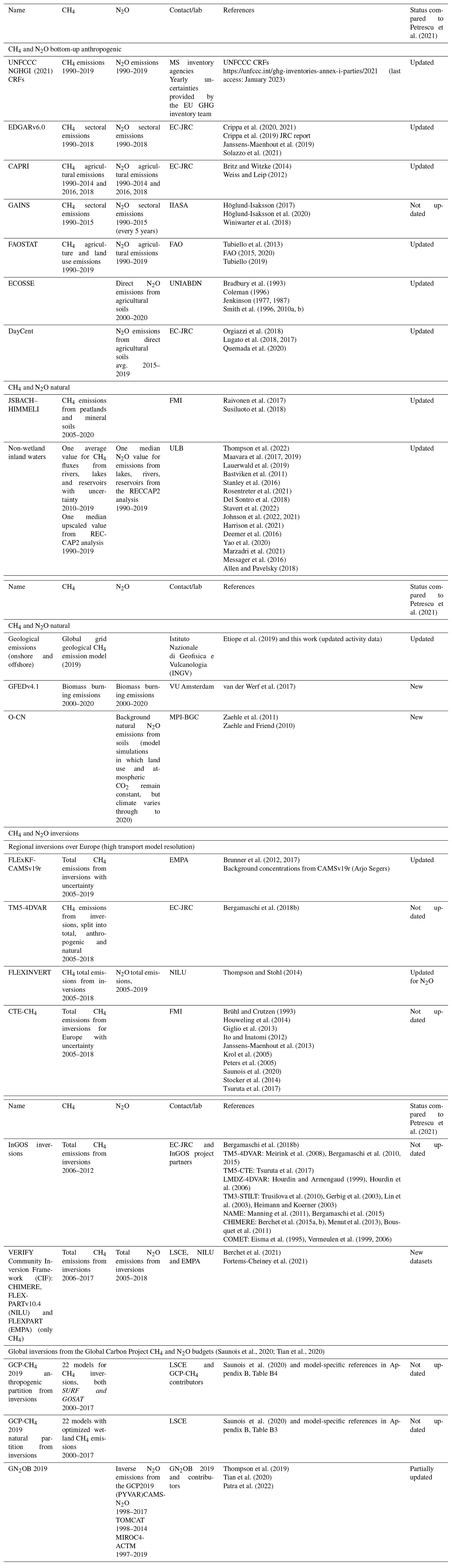
Total CH₄ fluxes from the EU27 + UK and five main regions in Europe – north, west, central, east (non-EU) and south – are presented in the paper. The countries included in these regions, which include countries outside the EU27 + UK bloc, are all Annex I parties to UNFCCC and are listed in Appendix A, Table A. Figure 1 shows the total CH₄ fluxes from the NGHGIs for base year 1990, as well as 5-year mean values for the 2011–2015 and 2015–2019 periods. The 5-year periods are informing on emission trends and what could be achieved by the GST process. Given that the GST is only repeated every 5 years, a 5-year average is clearly of interest even if in this current study 2021 estimates are not available. The total NGHGI estimates include emissions from all sectors (excluding LULUCF) and are plotted and compared to fluxes from global datasets, BU models and inversions. There is a good agreement noted in absolute total values between inventories, as well as between regional and global inversion ensembles, but uncertainties (min/max ranges) are large. This match can be explained by interdependencies in input data (activity data and emission factors, AD and EFs) for the BU estimates (Petrescu et al., 2020) and similar prior information used by inversions (Petrescu et al., 2021). In Fig. 1, hatched transparent bars represent the 2011–2015 mean while color-filled bars represent the new updated 2015–2019 mean values. For GAINS and some inversions that do not have annual estimates for all 5 years, only the average of available years is calculated (e.g., 2015 for GAINS).

For all study regions, 2019 CH₄ emissions decreased by 24 % (southern Europe) to 57 % (eastern Europe), with respect to NGHGI 1990 values; and for the EU27 + UK emissions decreased by 39 %. The decrease in CH₄ emissions is mainly due to the EU legislation policies and strategies starting with the implementation in the early 1990s of European and country-specific emission reduction policies on agriculture and the environment, as well as socioeconomic changes in the sector resulting in overall lower agricultural livestock and lower emissions from managed waste disposal on land and from agricultural soils. After 2005, these trends maintain their decreasing trajectory, even if at a lower intensity. For central and eastern Europe, reductions were abrupt and mainly due to the dissolution of the Soviet Union (1989–1991) and the consequent structural changes in the economy of the former eastern European communist centralized economy block (Petrescu et al., 2020). This is encouraging in the context of meeting EU total GHG commitments under the Paris Agreement (55 % decrease in 2030 compared to 1990 levels and reaching carbon neutrality by 2050). This reduction will need to be achieved by strong reductions in top emitter sectors (e.g., agriculture) and compensated for by sinks in the LULUCF sector. It also shows that not only at the EU27 + UK level, but also at the regional European level, the emissions from BU (anthropogenic and natural) and TD estimates agree in magnitude with reported NGHGI data despite the high uncertainty associated with the TD estimates. This uncertainty is represented here by the variability in the model ensembles and denotes the range (min and max) of estimates within each model ensemble. The comparison of TD to anthropogenic estimates (Fig. 1) suggests that the total CH₄ flux is dominated by natural emissions (i.e., northern Europe), although comparison with EDGARv6.0 would indicate that anthropogenic emissions are dominant (e.g., northern, central and western Europe).

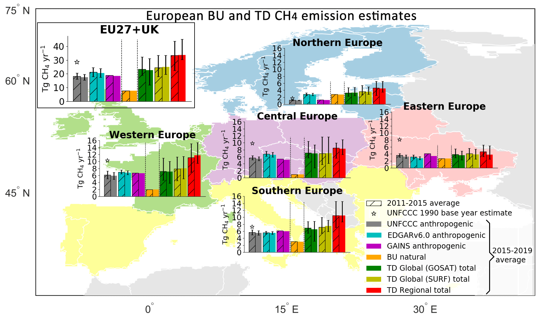
Figure 1 Five-year means (2011–2015, hashed bars, and 2015–2019, full bars) in total CH₄ emission estimates (excluding LULUCF) for the EU27 + UK and five European regions (north, west, central, south and east non-EU). The eastern European region does not include European Russia. Northern Europe includes Norway. Central Europe includes Switzerland. The data come from UNFCCC NGHGI (2021) submissions (gray), which are plotted with respective base year 1990 (black star) estimates, two inventories (GAINS and EDGARv6.0), natural unmanaged emissions (sum of peatland, geological, inland waters (RECCAP2) and GFEDv4.1 biomass burning emissions) and three inversion estimates: one regional European inversion (excluding InGOS unavailable for 2013–2015) and GOSAT and SURF ensemble estimates from global inverse models. The relative error on the UNFCCC value represents the UNFCCC NGHGI (2021) reported uncertainties computed with the error propagation method (95 % confidence interval) and gap-filled to provide respective estimates for each year. Uncertainty for EDGARv6.0 was calculated for 2015 based on the 95 % confidence interval of a lognormal distribution (Solazzo et al., 2021).

The EDGARv6.0 updated estimates for northern Europe remain 2 times higher than NGHGI and GAINS ones. The EDGAR approach is to use a globally harmonized methods and sources of data, which means that country-specific detail is often replaced with global averages. In some countries and for some sectors or gases, these assumptions lead to huge differences. For example, fugitive emissions of methane in the oil and gas sector are estimated based on the level of production of oil and gas. In the case of Norway this ignores the substantial effects of regulation on reducing such fugitive emissions. Instead, EDGAR's methane emission estimates for Norway follow the pattern of its total production of oil and gas (Olhoff et al., 2022). For eastern Europe we note that all estimates decreased compared to the previous 5-year mean, and the BU anthropogenic estimates remain similar in magnitude to the TD estimates of total CH₄ emissions. One possible explanation is that for TD estimates (i.e., using atmospheric inversions) the fluxes are better constrained by a larger number of observations. Where there are fewer or no observations, like in eastern Europe, the fluxes in the inversion will stay close to the prior estimates, since there is little or no information to adjust them.

In line with Bergamaschi et al. (2018b) the potentially significant contribution from natural unmanaged sources (peatlands, mineral soils, geological and inland waters, RECCAP2), which for the EU27 + UK accounted in 2019 for 8 Tg CH₄ yr⁻¹ (Fig. 1), can be highlighted. Taking into account these natural unmanaged CH₄ emissions and adding them to the range of the BU anthropogenic estimates (22 Tg CH₄ yr⁻¹ (NGHGI)–26 Tg CH₄ yr⁻¹ (EDGARv6.0)) improves agreement with the TD estimates. BU estimates become consistent with the lower range of the regional total TD estimates (32 Tg CH₄ yr⁻¹ (TM5_JRC)–41 Tg CH₄ yr⁻¹ (FLEXINVERT)) and show even better agreement in absolute values with the global median SURF (24 Tg CH₄ yr⁻¹) and GOSAT (23 Tg CH₄ yr⁻¹) inversions. The broad consistency between the TD and BU estimates could be interpreted in two ways: (1) BU and TD regional estimates are similar given the large uncertainties and spread in TD results or (2) regional TD higher estimates potentially indicate shortcomings of BU inventories, with the latter interpretation being more consistent with the general atmospheric developments (WMO, 2021).

Is it notable to highlight that the regional TD total is considerably higher for all regions and the EU27 + UK total, and by considering this estimate the best-to-date total estimate for the whole of Europe, including all sources and sinks, this would infer missing 20 % to 30 % of CH₄ emissions from the other BU approaches.

3.1.2 NGHGI sectoral emissions and decadal changes

According to the UNFCCC (2021) NGHGI estimates, in 2019 the EU27 + UK emitted GHGs totaling 3.7 Gt CO₂ eq. (including LULUCF); of this total, CH₄ emissions accounted for 11.8 % (0.4 Gt CO₂ eq. or 17.5±2.2 Tg CH₄ yr⁻¹) (Appendix B2, Fig. B2a), with France, the UK and Germany together contributing 37 % of total CH₄ emissions.

The data in Fig. 2 show anthropogenic CH₄ emissions and their change from one decade to the next, from UNFCCC NGHGI (2021), with the split between the different sectors. In 2019, NGHGIs report CH₄ from agricultural activities to be 52.4 % (±8.7 %) of the total EU27 + UK CH₄ emissions, followed by emissions from waste, 27.5 % (±22.5 %). The large share of agriculture in total anthropogenic CH₄ emissions also holds at the global level (IPCC, 2019). Between the 1990s and the 2000s, the net 17.6 % reduction originated largely from the energy and waste sectors, with only negligible contributions to emission trends and levels from IPPU (metal and chemical industry) and LULUCF. Between the 2000s and 2010–2019, a further reduction by 16.5 % was observed, with the waste sector being the largest contributor to this reduction. The two largest sectors contributing to total EU27 + UK emissions are agriculture and waste, but energy and waste have shown the higher reductions over the last decade.

The reduction observed in the waste sector coincides with the adoption of the first EU methane strategy published in 1996 (COM(96) 557, 1996). EU legislation addressing emissions in the waste sector may have been successful in triggering the largest reductions. Directive 1999/31/EC (1999) on the landfill (also referred to as the Landfill Directive) required the member states to separate waste, minimizing the amount of biodegradable waste disposed untreated in landfills, and to install landfill gas recovery at all new sites. Based on the 1999 directive, the new 2018/1999 EU Regulation on the Governance of the Energy Union requires the European Commission to propose a strategic plan for methane, which will become an integral part of the EU's long-term strategy. In the waste sector, the key proposal included the adoption of EU legislation requiring the installation of methane recovery and use systems at new and existing landfills. Other suggested actions included measures aimed at the minimization, separate collection and material recovery of organic waste (Olczak and Piebalgs, 2019).

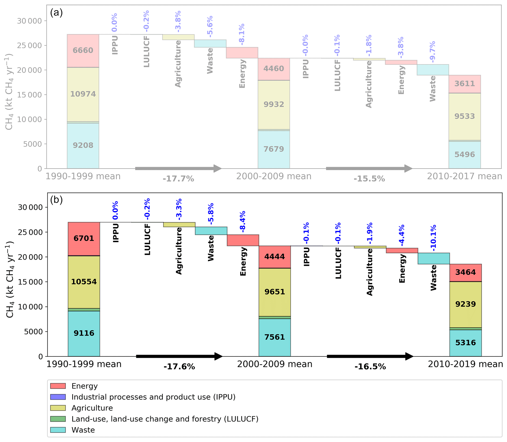
Figure 2 The contribution of changes (%) in CH₄ anthropogenic emissions in the five sectors to the overall change in decadal mean for the EU27 + UK, as reported to UNFCCC. Panel (a) shows the previous NGHGI data from Petrescu et al. (2021), and panel (b) illustrates data from UNFCCC NGHGI (2021). The three stacked columns represent the average CH₄ emissions from each sector during three periods (1990–1999, 2000–2009 and 2010–2019), and percentages represent the contribution of each sector to the total reduction percentages (black arrows) between periods.

3.1.3 NGHGI estimates compared with bottom-up inventories

The data in Fig. 3 present the total anthropogenic CH₄ emissions from four BU inventories and UNFCCC NGHGI (2021) submissions excluding emissions from LULUCF, which was identified as a non-significant contributor (Fig. 2). According to NGHGI, in 2019 anthropogenic CH₄ emissions from the four sectors (Table 1, excluding LULUCF) amounted to 17.1 Tg CH₄ yr⁻¹, representing 10.5 % of the total EU27 + UK GHG emissions in CO₂ eq. Figure 3a shows EDGARv6.0 and GAINS trends being consistent with the ones of NGHGI (excluding LULUCF), although GAINS and NGHGI agree in terms of emission levels. EDGARv6.0 estimates are consistently higher estimates (∼19 %) than NGHGI. In contrast to the previous version, EDGARv4.3.2, which was found by Petrescu et al. (2020) to be consistent with UNFCCC NGHGI (2018) data, EDGARv6.0 reports higher estimates than EDGARv5.0 (∼8 % higher) and falls outside the 9.6 % UNFCCC uncertainty range. Over the 1990–2019 period, the trends in emissions agree well between the two BU datasets and NGHGI, showing linear trend reductions of 40 % for EDGARv6.0 and 36 % for GAINS and NGHGIs. The average yearly reduction trend was 2 % yr⁻¹ for all three data sources.

Figure 3 Total annual anthropogenic CH₄ emissions (excluding LULUCF) for the EU27 + UK over time. The top plot presents previous data synthesized in Petrescu et al. (2021), while the bottom plot shows data synthesized by the current study: (a) EU27 + UK and total sectoral emissions from (b) energy, (c) industrial processes and product use (IPPU), (d) agriculture, and (e) waste from UNFCCC NGHGI (2021) submissions compared to global bottom-up inventory models for agriculture (CAPRI, FAOSTAT) and all sectors excluding LULUCF (EDGARv6.0, GAINS). CAPRI reports one estimate for Belgium and Luxembourg. The relative error on the UNFCCC value represents the UNFCCC NGHGI (2021) member-state-reported uncertainties computed with the error propagation method (95 % confidence interval) that were gap-filled and provided for every year. The uncertainty for EDGARv6.0 is the same as that of v5.0 and calculated for 2015 as min/max values for the total and each sector (Solazzo et al., 2021) and represents the 95 % confidence interval of a lognormal distribution. The mean column represents the common overlapping periods between datasets: 1990–2015 for total EU27 + UK, energy, agriculture and waste; 1990–2018 for IPPU; and 1990–2014 for CAPRI. The last years of the time series of the respective datasets are 2018 (EDGARv6.0, CAPRI), 2019 (FAOSTAT, UNFCCC) and 2015 (GAINS). After 2014 CAPRI delivered estimates for 2 additional years, 2016 and 2018, as well as uncertainties for 2014 and 2018 (25.1 %) and 2016 (25.2 %).

Sectoral time series of anthropogenic CH₄ emissions (excluding LULUCF) and their means are shown in Fig. 3b–e. For the energy sector (Fig. 3b), both EDGARv6.0 and GAINS agree in trends with the NGHGI thanks to updated methodology that derives emission factors and accounts for country-specific information about associated petroleum gas generation and recovery, venting and flaring (Höglund-Isaksson, 2017). After 2005, GAINS reports consistently lower emissions than UNFCCC due to a phasedown of hard coal production in the Czech Republic, Germany, Poland and the UK; a decline in oil production in particular in the UK; and declining emission factors reflecting reduced leakage from gas distribution networks as old town gas networks are replaced. A difference in tiers is also one reason for the differences (Petrescu et al., 2020).

The consistently higher estimates (+6 % compared to the UNFCCC mean) of EDGARv6.0 might be due to the use of default emission factors for oil and gas production based on data from the US (Janssens-Maenhout et al., 2019). There are several other reasons that could be the cause for the differences, including the use of Tier 1 emission factors for coal mines, assumptions for material in the pipelines (in the case of gas transport) and the activity data. Also EDGARv6.0, similar to the previous estimates from EDGARv5.0, uses the gas pipeline length as a proxy for the activity data; however, this may not be appropriate for the case of the official data, which could consider the total amount of gas being transported or both methods according to the countries. Using pipeline length may overestimate the emissions because the pipeline is not always at 100 % capacity; thus, a larger amount of methane is assumed to be leaked (Rutherford et al., 2021). For coal mining, emissions are a function of the different types of processes being modeled.

The IPPU sector (Fig. 3c), which has only a small share of the total emissions, is not included in GAINS, while EDGARv6.0 estimates are less than half of the emissions reported by NGHGI 2021 in this sector. The discrepancy for this sector has a negligible impact on discrepancy for the total CH₄ emission. However, we identified that the low bias of EDGARv6.0 could be explained by fewer activities included in EDGARv6.0 (e.g., missing solvent, electronics and other manufacturing goods) accounting for 5.5 % of the total IPPU emissions in 2015 reported to UNFCCC. The reason for the remaining difference could be explained by the allocation of emissions from auto-producers⁵ in EDGARv6.0 to the energy sector (following the 1996 IPCC guidelines), while in NGHGI they are reported under the IPPU sector (following the 2006 IPCC guidelines).

As CAPRI and FAOSTAT report only emissions from agriculture, they are included only in Fig. 3d. The data (EDGARv6.0, GAINS, CAPRI and FAOSTAT) show good agreement, with CAPRI at the lower range of emissions (Petrescu et al., 2020) and on average 3 % lower than that of NGHGI and with EDGARv6.0 at the upper range. The reason for EDGARv6.0 having the highest estimate (contrary to Petrescu et al., 2020, where NGHGIs were the highest and EDGARv4.3.2 was the second highest) is likely due to the activity data updates in EDGARv6.0 based on FAOSTAT values, compared to EDGARv4.3.2. When looking at the time series mean, EDGARv6.0, GAINS and FAOSTAT show 5 % higher emissions than that of NGHGI. The three BU estimates and NGHGI estimates show similar mean values likely due to the use of similar activity data and emission factors (EFs) (i.e., Fig. 4 in Petrescu et al., 2020). The updates submitted by CAPRI, for the years 2014, 2016 and 2018, match the NGHGI emission estimates and have uncertainties of 21 %. Compared to the previous version of CAPRI used in Petrescu et al. (2021), the new runs report lower CH₄ emissions. Compared to previous results, some changes have been implemented in the last version (e.g., introduction of slope and altitude limits based on LUCAS⁶ and improved distribution of grazing livestock, among others). The main activity triggering the differences was the emissions from enteric fermentation. Statistical information on most agricultural data required for the estimation of CH₄ and N₂O emissions is not available at high spatial (regional) and temporal (annual since 1990) resolution. Therefore, the CAPRI model features a module that provides generic data at the regional level (CAPREG) and additionally a module that also estimates feed distribution and GHG emissions at the required resolution for VERIFY (CAPINV). As indicated in an internal VERIFY report (Leip, 2019), the results of the CAPINV module were scrutinized and shortcomings were identified. These concern mainly the distribution of feed, which is one of the most important parameters for CH₄ emissions from enteric fermentation, and manure excretion and subsequent GHG emissions. Other updates included addition of some regional input data (sources: FAOSTAT and EUROSTAT).

For the waste sector (Fig. 3e) EDGARv6.0 shows consistently higher estimates compared to the NGHGI data, while GAINS has higher emissions than the NGHGI after 2000 (mean 1990–2015 value 6 % higher than NGHGI emissions). The two inventories, EDGARv6.0 in its 2020 update for landfills and GAINS, used an approach based on the decomposition of waste into different biodegradable streams, with the aim of applying the methodology described in the 2019 refinement to the 2006 IPCC guidelines and the IPCC waste model (IPCC, 2019) using the first-order-decay (FOD) method. The main differences between the two datasets come from (i) sources for total waste generated per person, (ii) the assumption for the fraction composted and (iii) the oxidation. The two inventories may have used different strategies to complete the waste database when inconsistencies were observed in the EUROSTAT database or in the waste emission trends in NGHGI.

3.1.4 NGHGI estimates compared to atmospheric inversions

European estimates from regional inversions

Figure 4 compares TD regional estimates, NGHGI anthropogenic data for CH₄ emissions and natural BU emissions. Figure 4a presents TD estimates of total emissions (anthropogenic and natural) from Petrescu et al. (2021), while Fig. 4b shows the current study with updated total TD estimates. Figure 4c and d show estimates of anthropogenic emissions (Petrescu et al., 2021, and current study) calculated by subtracting the total natural emissions from the total TD emissions.

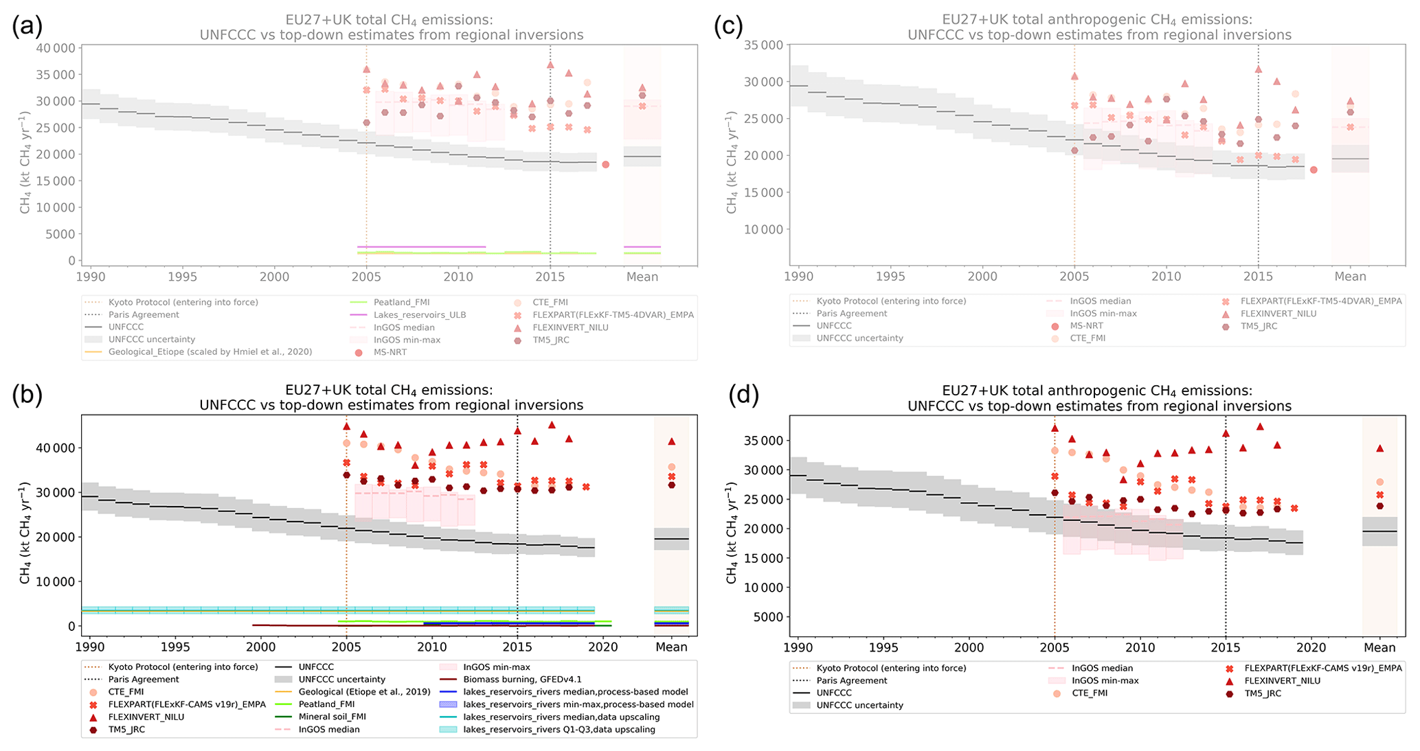
Figure 4 (a, b) Comparison of total CH₄ emissions for the EU27 + UK from four top-down regional inversions with UNFCCC NGHGI (gray) data and two estimates for inland waters (lake, river and reservoir process-based models, blue, and upscaled emissions, cyan), peatlands and mineral soils (from JSBACH–HIMMELI, light green and dark green), geological emissions (orange), and biomass burning (from GFEDv4.1, brown) as follows: (a) previous data from Petrescu et al. (2021), current study. (c, d) Comparison of anthropogenic CH₄ emissions from four top-down regional inversions with UNFCCC NGHGI (gray) data as follows: (c) previous data from Petrescu et al. (2021), current study. Anthropogenic emissions from these inversions are obtained by removing natural emissions and biomass burning from total TD CH₄ emissions shown in Fig. 4a and b. UNFCCC NGHGI (2021) reported uncertainties computed with the error propagation method (95 % confidence interval) were calculated for each year of the time series and represent the gap-filled harmonized member-state-reported uncertainty for all sectors (including LULUCF). The time series mean was computed for the common period of 2005–2018 between datasets (excluding InGOS).

The TD estimates of European CH₄ emissions in Fig. 4b use four European regional models for the 2005–2018 period and an ensemble of five different inverse models (InGOS, Bergamaschi et al., 2015) for 2006–2012.

For the 2005–2018 period (excluding InGOS), the four regional inversions give a total CH₄ emission mean of 36 (32–42) Tg CH₄ yr⁻¹ compared to anthropogenic total of 20 Tg CH₄ yr⁻¹ in NGHGI (Fig. 4b). The large positive difference between TD and NGHGI suggests a potentially significant contribution from BU natural sources, represented separately in Fig. B2, Appendix B1 (peatlands, geological sources, inland waters and biomass burning), which for the same period are estimated at 8 Tg CH₄ yr⁻¹. However, it needs to be emphasized that natural wetland emission estimates have large uncertainties and show large variability in the spatial (seasonal) distribution of CH₄ emissions, but for Europe their inter-annual variability is not very strong (mean of 14 years from JSBACH–HIMMELI peatland emissions is 1.0 Tg CH₄ yr⁻¹). Overall, they do represent an important source and could dominate the budget assessments in some regions such as northern Europe (Fig. 1). That TD and NGHGIs diverged in terms of both emission levels and trends is certainly significant and potentially has implications for bottom-up and NGHGI estimates of CH₄ emissions, if the discrepancies cannot be explained by natural fluxes alone.

The differences between inversion results in the current study and Petrescu et al. (2021) can be summarized as follows: for the version used in this study, FLExKF-CAMSv19r_EMPA, the background mole fraction was taken from a global CAMSv19r assimilation run with assimilation of surface observations of CH₄ only (no satellite data) where the domain was cut out following the two-step approach of Rödenbeck et al. (2009). Background concentrations from CAMSv19r are on average about 5 ppb lower than those of the TM5-4DVAR system used previously, which results in somewhat higher emission estimates over Europe compared to Petrescu et al. (2021). The major differences to the previous CTE-FMI run are the prior fluxes, except for biomass burning, which remained GFED. The new VERIFY_S5 (core) run uses fluxes as described in Thompson et al. (2022). The new VERIFY_S5 (core) run uses fluxes as described in Thompson et al. (2022). Lake and geological emissions were not included in the Petrescu et al. (2021) synthesis but are included in the current CTE-FMI simulation, which probably also contributes to higher total emissions. On top of this, the assimilated data (i.e., observation network) contributes to the differences (enlarged observation network, more sites – five core sites for CH₄ located in Spain, France and the UK were added). The FLEXINVERT version used in this study updated the atmospheric observation network (more sites were added) as well as the prior emissions. The background mole fraction was also coupled with that from the CAMSv19r assimilation run, which, similar to the FLExKF model, might imply higher emissions. Regarding decreasing trends seen for the current inversion CH₄ results, for the FLExKF model the trend in CH₄ emission was slightly negative over 2005–2019, at −0.48 % per year, which is lower than the decrease in the prior of −0.8 % per year. For the other models, based on Thompson et al. (2022), the differences in trends might be due to regional vs. global inversion differences.

The geological emissions were recalculated based on the global grid model of Etiope et al. (2019), using more precise “activity” data for the EU27 + UK (details in Appendix A2): the emission results were 3.3 Tg CH₄ yr⁻¹, i.e., 42 % of the total natural CH₄ emissions in the EU27 + UK. Geological emissions are an important component of the EU27 + UK emissions budget, but their temporal variability is unknown (Etiope and Schwietzke, 2019), and so their impact on climate warming cannot be predicted.

The other natural sources of CH₄ contribute as follows: natural emissions from inland waters (RECCAP2) contribute 3.4 Tg CH₄ yr⁻¹, or 43 % of the total natural CH₄ emissions; peatlands and mineral soils (Raivonen et al., 2017; Susiluoto et al., 2018) account for 1.0 Tg CH₄ yr⁻¹, i.e., 13.4 % of the total natural CH₄ emissions, while biomass burning contributes only 0.6 % to the total CH₄ natural emissions.

Similar to peatlands, inland water emissions also remain highly uncertain. The compilation of emission estimates leads to a total flux that is 3.3 Tg CH₄ yr⁻¹ (min 2.7 Tg CH₄ yr⁻¹ and max 4.3 Tg CH₄ yr⁻¹) and about 5 times larger than the process-based model estimates for lakes + reservoirs and the spatially resolved flux for rivers (0.6 Tg CH₄ yr⁻¹ with min 0.2 and max 0.8 Tg CH₄ yr⁻¹) and about 25 % larger than the previous budget in Petrescu et al. (2021) (2.5 Tg CH₄ yr⁻¹), which ignored the contribution of rivers and relied on one observation-based estimate (extrapolation from late-summer data reported in Rinta et al., 2017) and four semi-empirical model assessments (Petrescu et al., 2021). Interestingly, the new process-based estimate for natural lake + reservoirs CH₄ emissions matches well the data-driven assessment by Rinta et al. (2017) for the late-summer season, with a relative difference smaller than 5 %.

The RECCAP2 approach synthesizes 15 average annual CH₄ emissions fluxes for Europe (Rosentreter et al., 2021; Bastviken et al., 2011; Del Sontro et al., 2018; Stavert et al., 2022; Johnson et al., 2022, 2021; Harrison et al., 2021; Deemer et al., 2016) that were homogenized and rescaled to a consistent set of inland water surface area (Messager et al., 2016; Allen and Pavelsky, 2018) and corrected for the effect of seasonal ice cover (Yang et al., 2020).

Model results, however, also reveal a strong seasonal variability in CH₄ emissions, with much lower fluxes during winter. This seasonality is driven by physical factors (changing ice cover and bottom-water temperature) and biogeochemical factors (autotrophic primary production) that are well-established drivers of the temporal variability in lake CH₄ emissions (Del Sontro et al., 2018; Jansen et al., 2022). This finding provides a likely explanation as to why the spatiotemporally resolved model results lead to significantly lower estimates than observation-based methods that do not capture well the temporal variability in lake CH₄ emissions.

According to the IPCC 2006 guidelines (IPCC, 2006) CH₄ emissions from wetlands are reported by the member states to the NGHGI under the LULUCF sector and considered anthropogenic, if the wetlands in question are considered managed land. They are included in the total LULUCF values (Figs. 1, 2, 4 and 6), and in 2019 reported CH₄ emissions from wetlands accounted for 0.1 Tg CH₄ yr⁻¹.

To quantify the anthropogenic CH₄ component in the European TD estimates, the BU peatland emissions from the regional JSBACH–HIMMELI model and those from geological, inland water sources and biomass burning were subtracted from the total TD emissions (Fig. 4d). It remains, however, uncertain to perform these corrections due to the prior inventory data allocation of emissions to different sectors (e.g., anthropogenic or natural) used in inversions, which can induce uncertainty of up to 100 % if, for example, an inventory allocates all emissions to natural emissions and the correction is made by subtracting the natural emissions. All regional inversion anthropogenic estimates are higher compared to the UNFCCC NGHGI (2021) mean of 28 Tg CH₄ yr⁻¹ from inversions compared to 20 Tg CH₄ yr⁻¹ from the NGHGIs. Regarding trends, TD emissions are stable except for CTE showing a linear decreasing trend up to 2015 followed by an increase over the next 3 years, while NGHGIs and BU trends are declining. From this attempt we find that not many of the inversions showed the clear decline reported by the NGHGIs. As NGHGI emissions are dominated by anthropogenic fluxes and decline by almost 30 % compared to 1990, a similar decline was expected in the corrected anthropogenic inversions. Further investigation into how well the NGHGIs reflect reality or how well the TD estimates capture the trends is clearly needed. Currently, in the UNFCCC UK NIR (https://unfccc.int/documents/273439, last access: December 2022) the national inversion system produced similar recent UK CH₄ emission levels but did not validate the large declining trend since 1990 that is estimated by the UK inventory.

Spatial distribution of CH₄ emissions from regional inversions

A novelty in this study is represented by the fact that new top-down estimates of CH₄ fluxes were also calculated in this reporting period using the Community Inversion Framework (CIF) (Berchet et al., 2021). For CH₄ (Fig. 5), inversions using three atmospheric transport models (or model variants) were performed with the CIF: (i) the regional non-hydrostatic Eulerian model, CHIMERE (Fortems-Cheiney et al., 2021), used by LSCE; (ii) the Lagrangian particle dispersion model, FLEXPART, used by EMPA (from hereon, FLEXPART-EMPA); and (iii) FLEXPART used by NILU (from hereon, FLEXPART-NILU).

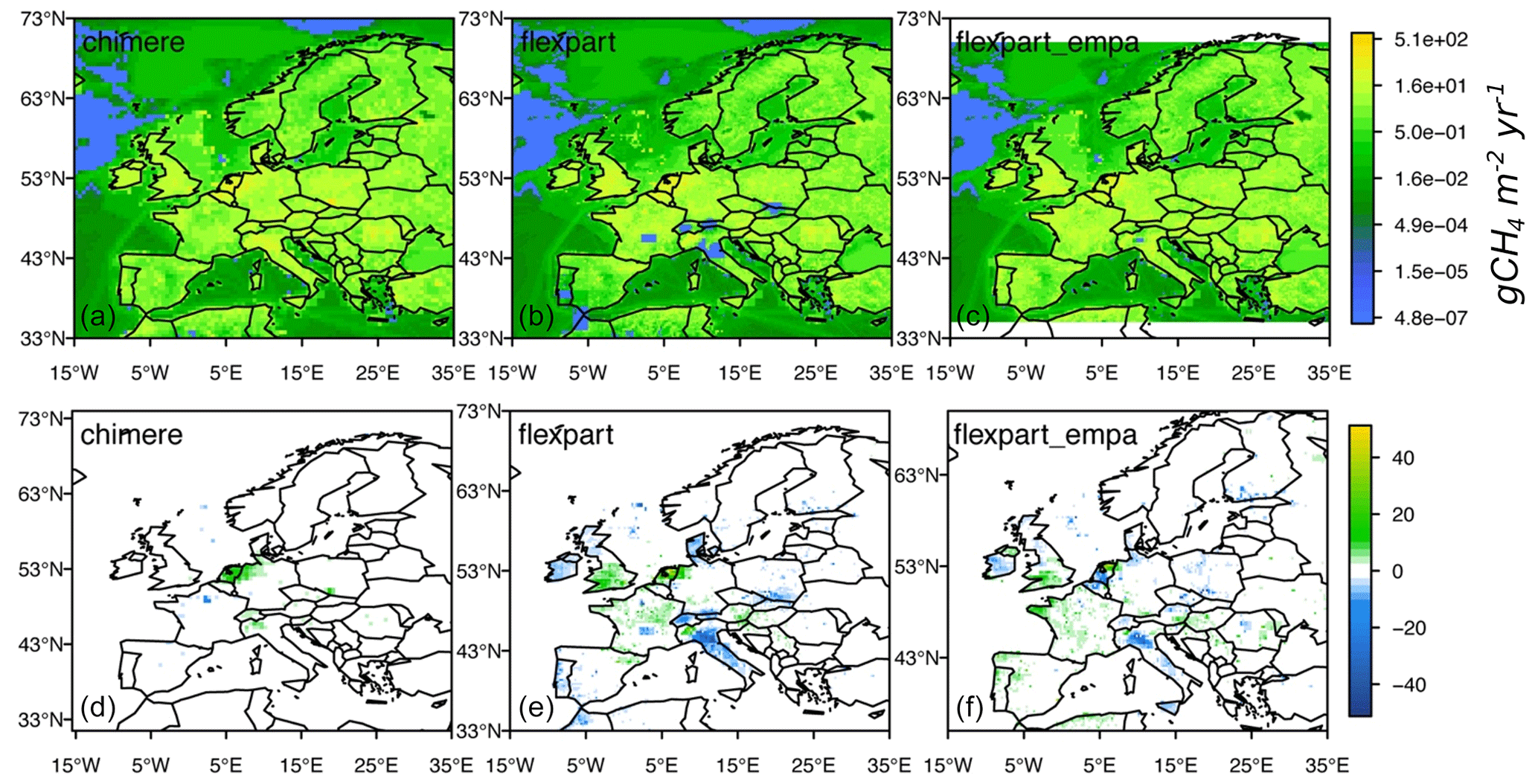
Figure 5 Posterior CH₄ fluxes averaged over 2006–2017 (g CH₄ m⁻² yr⁻¹) from three regional inversions, CHIMERE (LSCE), FLEXPART (NILU) and FLEXPART (EMPA), shown with a log-base-2 color scale (a–c) and the flux increments (posterior-prior) (g CH₄ m⁻² yr⁻¹) shown on a linear color scale (d–f).

The spatial distribution of CH₄ fluxes are similar for the three inversions with higher emissions in the Netherlands and Belgium, western France, and the southern UK. However, FLEXPART-NILU inversions show some spurious areas of very low fluxes in Italy, Switzerland and southern France, which are presumably owing to the positive bias in the prior modeling mixing ratios at mountain sites, which will be corrected in future simulations. The patterns of differences, however, are quite different between the CHIMERE and the two FLEXPART inversions. All inversions find positive increments (posterior high than prior) over the northern Netherlands, but FLEXPART-EMPA finds negative increments over the southern Netherlands, and both FLEXPART inversions find negative increments over northern Italy, which is not the case in CHIMERE (Fig. 5, top). The total mean emissions for the EU27 + UK over 2006–2017 (Fig. 5) were 26, 22 and 24 Tg CH₄ yr⁻¹, for CHIMERE, FLEXPART-NILU and FLEXPART-EMPA, respectively. FLEXPART-EMPA is the same model as used in the comparison shown in Fig. 4 (FLEXPART(FLExKF-CAMSv19r)), but in those inversions the total mean emissions for the EU27 + UK were higher at 33 Tg yr⁻¹. This difference is likely owing to the different dataset used for determining the background mixing ratios, and further analysis is ongoing.

European estimates from global inversions

Figure 6 compares TD global estimates with NGHGI data and provides information about the wetland emissions from global wetland inversions (Saunois et al., 2020). Figure 6a presents TD estimates of total emissions (anthropogenic and natural) from Petrescu et al. (2021), while Fig. 6b shows the current study with updated total TD estimates. Figure 6c and d show estimates of anthropogenic emissions (Petrescu et al., 2021, and current study) calculated by subtracting the total natural emissions from the global total TD emissions.

The global inversion models were split according to the type of observations used, 11 of them using satellites (GOSAT) and 11 using surface stations (SURF). Each of these 22 global inversions provided as well wetland emissions used by the Global Methane Budget (Saunois et al., 2020) and is post-processed with prior ratio estimates for wetland CH₄ emissions (Appendix B2, Table B4).

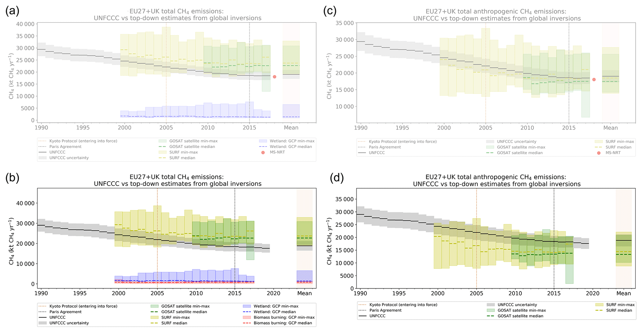
Figure 6 (a, b) Total CH₄ emissions from TD global ensembles based on surface station data (SURF) (yellow) and satellite concentration observations (GOSAT) (green) from 22 global models compared with UNFCCC NGHGI (gray) data (including LULUCF) as follows: (a, c) previous data from Petrescu et al. (2021) and (b, d) the current study. (c, d) Anthropogenic CH₄ emissions from top-down global inversions based on surface stations (SURF) (yellow) and on satellite concentration observations (GOSAT) (green) from different estimates as follows: (c) previous data from Petrescu et al. (2021) and (d) the current study. Anthropogenic emissions from these inversions were obtained by removing the sum of the natural emissions (global wetland GCP emissions (blue), the inland waters and geological fluxes as shown in Fig. 4a) from the total estimates. The biomass burning emissions included in each inversion result were removed as well. UNFCCC NGHGI (2021) member-state-reported uncertainty computed with the error propagation method (95 % confidence interval) was gap-filled and provided for every year for all sectors (including LULUCF). The time series mean was computed for the common period of 2010–2016. Two out of 11 SURF products (GELCA-SURF_NIES, TOMCAT-SURF_UOL) were not available for 2016.

For the common period between datasets (2010–2016), the two ensembles of regional and global models give a total CH₄ emission mean (Fig. 6a) of 23 Tg CH₄ yr⁻¹ (GOSAT) and 24 Tg CH₄ yr⁻¹ (SURF) for the EU27 + UK compared to 19±2.3 Tg CH₄ yr⁻¹ of NGHGI (Fig. 6a). The mean of the natural wetland emissions from the global inversions is 1.3 Tg CH₄ yr⁻¹ and partly explains the positive difference between total emissions from inversions and NGHGI anthropogenic emissions.

To quantify the European TD anthropogenic CH₄ component, the GCP inversion wetland emissions and those from geological, inland water sources and biomass burning emissions (reported by the global inversions) were subtracted from the total CH₄ emissions (Fig. 6d).

For the 2010–2016 common period, the two ensembles of global models give an anthropogenic CH₄ emission median (Fig. 6b) of 13 Tg CH₄ yr⁻¹, with min and max values of 10 and 21 Tg CH₄ yr⁻¹ (GOSAT), and 14 Tg CH₄ yr⁻¹, with min and max values of 9 and 22 Tg CH₄ yr⁻¹ (SURF), compared to 19±2.3 Tg CH₄ yr⁻¹ for NGHGI. The TD ensemble that produced the closest anthropogenic estimate (Fig. 6d) to the UNFCCC NGHGI (2021) is SURF, with the median of SURF inversions falling just below the uncertainty range of the NGHGI.

Between 2010–2016, total TD CH₄ emissions (Fig. 6b) from the SURF and GOSAT ensemble decreased by 0.5 % and 4.6 %, respectively. For anthropogenic CH₄ emissions (Fig. 6d), the SURF and GOSAT ensembles show a decrease of 1.1 % and 6.3 %, respectively, compared to the 7.7 % decrease for the NGHGI.

3.1.5 CH₄ uncertainty reduction maps

Bergamaschi et al. (2010) used TM5 4DVAR to analyze the sensitivity of the modeling system to observations, for further interpretation of the derived emissions, in particular in the context of verification of BU inventories. For this purpose, Bergamaschi et al. (2010) calculated uncertainty reduction maps, as a measure of the sensitivity of the observational network used for the reference inversion. This reduction in uncertainty is calculated as the ratio between a posterior and a prior uncertainty with the formula (1−Δpost $/\mathrm{\Delta }$prior), where Δpost represents the posterior uncertainties and Δprior the prior uncertainties of the inversion system. The same methodology was applied to two VERIFY regional inversions systems, CTE-CH₄ and FLExKF (Brunner, 2022).

The first inversion system, FLExKF, calculated the uncertainty reduction maps for CH₄ for the year 2018 with two different sets of observation stations (Fig. 7). Maps of uncertainty reduction can be really informative, and the results below (Fig. 7) present the uncertainty reductions for two different sets of stations, which show the value of only considering ICOS sites (left figure) and when adding also other stations in the UK and Switzerland (right figure).

Figure 7 FLExKF uncertainty reduction maps computed as (1−Δpost $/\mathrm{\Delta }$prior) for the same year, 2018, but with two different sets of observation stations (white dots).

However, the larger the prior uncertainties, the stronger the potential for uncertainty reduction is; therefore, given that the prior uncertainty varies, the uncertainty reduction is not a direct indication of the information provided by observations. The second inversion system, CTE-CH₄ (Tsuruta et al., 2017), calculated the uncertainty reduction maps from surface inversions (SURF) for 2006 and 2018, as those used in Thompson et al. (2022), referred to here as VERIFY_S5 (core inversion) (Fig. 8). The system included two sets of inversions with different observation sets assimilated. However, the degrees of freedom in the state of the system were low, and, therefore, the uncertainty estimates may not differ much between the two. The data from CTE-CH₄ include uncertainties (standard deviations) and fluxes for 2006 and 2018. The differences in the simulations are observation sets and the underlying prior covariance structure. VERIFY_S5 uses data from only those sites that have long-term measurements assimilated; i.e., there is little difference in the assimilated sites between the years. From the two panels of Fig. 8, higher uncertainty reductions are seen in 2018 compared to 2006 in E Poland, N Italy and Spain.

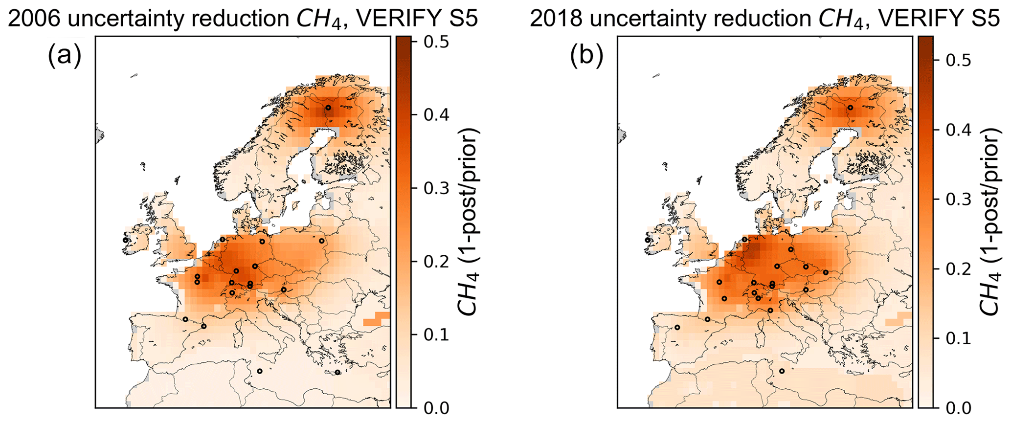
Figure 8 VERIFY_S5 (core) inversion run; uncertainty reduction maps computed as (1−Δpost $/\mathrm{\Delta }$prior) for 2006 (a) and 2018 (b) with different sets of observation stations.

The differences between the 2 years are mostly due to changes in the amount of observational data, although additional observation stations in certain locations may produce only a limited reduction in uncertainty. This can occur if (i) uncertainty assigned to the observations (i.e., how much weight/trust we put in it) is comparatively high, (ii) prior emissions and/or their uncertainties around the sites are simply very small and therefore the inversion does not change fluxes much, and/or (iii) the location is not very sensitive to emissions in the surrounding area (e.g., mountain sites) due to the atmospheric transport to the observation site. Generally, sites that contribute to a larger uncertainty reduction should be included in the inversions and located closer to emission sources and/or sink areas.

CTE-CH₄ was also used to estimate fluxes utilizing prior information from GOSAT data, for 2010 and 2017. Figure 9 presents the associated uncertainty reduction maps. Because of the different inversion system setup (e.g., resolution, spatial correlation) compared to previous results, where prior data were coming from observation networks, it is difficult to conclude what effects satellites have on posterior emissions from the 2 years. However, it is interesting to note how satellite data assimilation infers changes on a regional scale. Unlike surface stations, satellite data have more power to constrain northern European emissions than central European emissions.

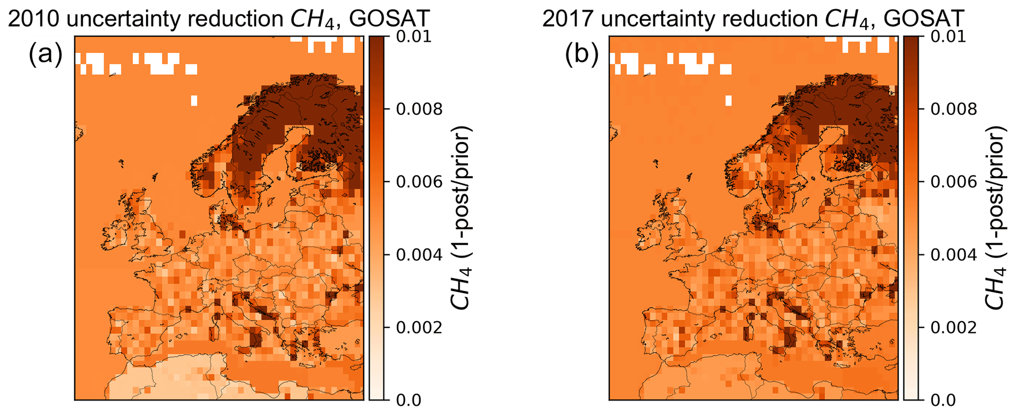
Figure 9 CTE-CH₄ GOSAT inversion run; uncertainty reduction maps computed as (1−Δpost $/\mathrm{\Delta }$prior) for 2010 (a) and 2017 (b).

3.2 Comparing N₂O emission estimates from different approaches

3.2.1 Estimates of European and regional total N₂O fluxes

Total N₂O fluxes from the EU27 + UK and five main regions in Europe are presented in a similar fashion as the CH₄. Figure 10 summarizes the total N₂O fluxes from NGHGI 2021 (excluding LULUCF) for the base year 1990 as well as mean annual emissions for the 2011–2015 and 2015–2019 5-year periods.

The total UNFCCC estimates that include emissions from all sectors are compared with the fluxes from global datasets, BU models and TD inversions. Relative to 1990, N₂O emissions in 2019 decreased by a minimum of 26 % (eastern Europe) up to a maximum of 46 % (western Europe) and by 39 % for the EU27 + UK. At the European level, the emissions from BU estimates (anthropogenic NGHGI plus the sum of all natural, 991 kt N₂O) and the TD total (including natural) regional estimate (1443 kt N₂O) averaged over 2015–2019 roughly agree within the uncertainty reported by UNFCCC (±59 %). The TD uncertainty is represented as the variability in the model ensembles and denotes the range between the minimum and maximum estimates within each model ensemble. There is significant uncertainty in northern Europe, where the TD average estimates indicate sources, yet the ensemble ranges from a net sink to a net source (Fig. 10). The current observation network is sparse, which currently limits the capability of inverse models to quantify N₂O emissions at the country or regional scale.

For all other regions, the BU anthropogenic emissions agree in absolute values with the NGHGI given uncertainties, though consistently higher estimates are produced by TD regional and global models. The difference is still too high to be attributed to the sum of the natural emission, which ranges for all five regions in 2019 between a minimum of 13 kt N₂O yr⁻¹ (northern Europe) to a maximum of 113 kt N₂O yr⁻¹ (southern Europe), while the EU27 + UK total natural emission is estimated at 178 kt N₂O yr⁻¹.

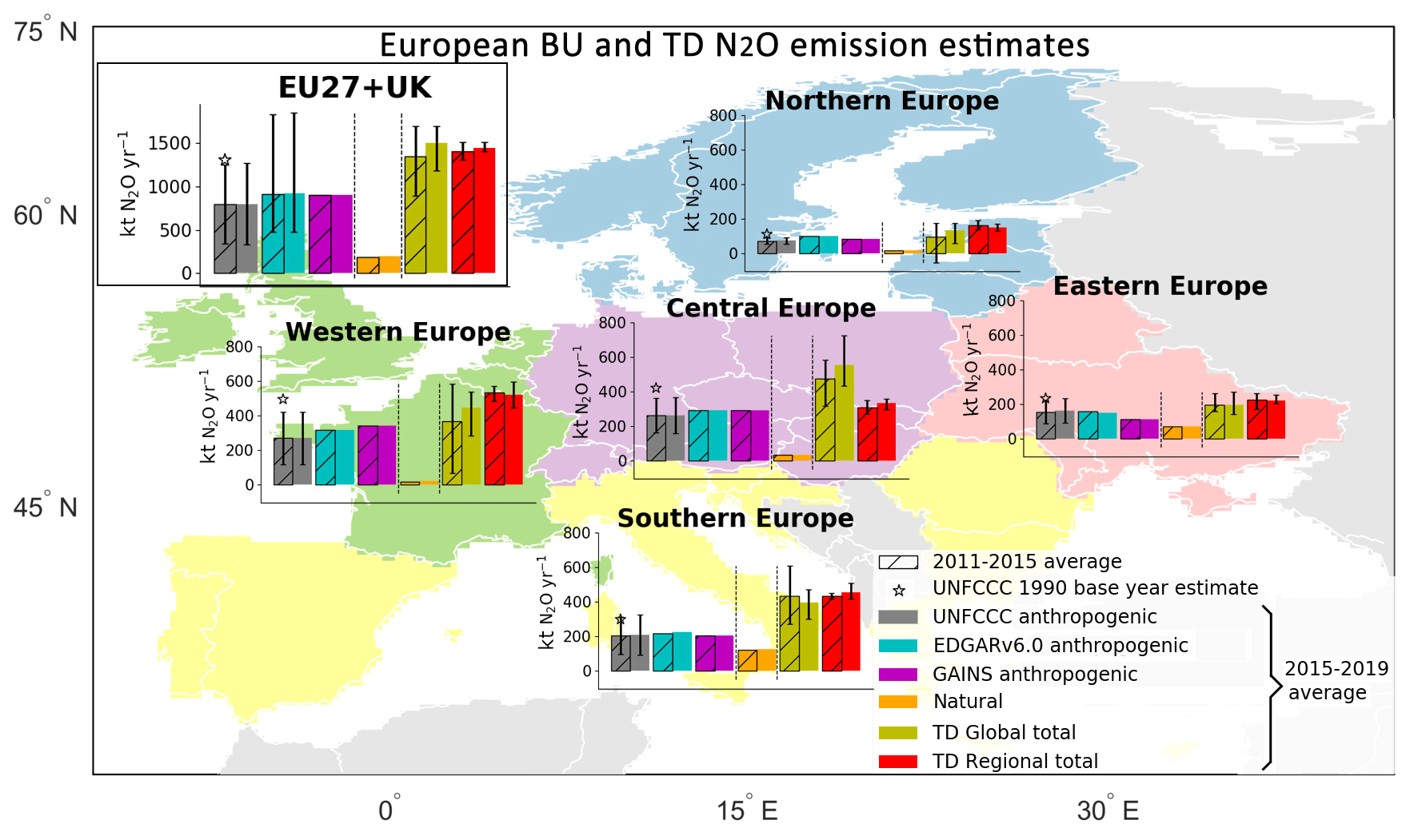
Figure 10 Five-yearly means (2011–2015 hashed bars and 2015–2019 full bars) in total N₂O emission estimates (excluding LULUCF) for the EU27 + UK and five European regions (northern, western, central, southern and eastern non-EU). The eastern European region does not include European Russia, northern Europe includes Norway and central Europe includes Switzerland. The data are from the UNFCCC NGHGI (2021) submissions (gray), which are plotted with respective base year 1990 (black star) estimates; two inventories (GAINS and EDGARv6.0); natural unmanaged emissions (lake, river and reservoir emissions from RECCAP2 and natural N₂O from O-CN); and two inversion total estimates (one regional European inversion (FLEXINVERT) and the average of three global inverse models from GN₂OB, Tian et al., 2020). The relative error on the UNFCCC value represents the NGHGI (2021) reported uncertainties computed with the error propagation method (95 % confidence interval) and gap-filled to provide respective estimates for each year (see Appendix A); for eastern Europe non-EU the uncertainty value of 42.3 % was calculated from the NIRs. Northern Europe Tier 1 uncertainty for Norway was not available.

3.2.2 NGHGI sectoral emissions and decadal changes

According to the UNFCCC NGHGI (2021) estimates for 2019, the EU27 + UK emitted GHGs totaling 3.7 Gt CO₂ eq. (including LULUCF, using a GWP 100, IPCC AR4) (Appendix B1, Fig. B1, right), of which N₂O emissions accounted for ∼7 % (254 Mt CO₂ eq. or 854 kt N₂O yr⁻¹) (Fig. 11). France, Germany and the UK together contributed 40 % of total N₂O emissions (338 kt N₂O yr⁻¹). For 2019, NGHGI reported anthropogenic emissions from the EU27 + UK for the four activity sectors (excluding LULUCF) (Table 1) to be 793 kt N₂O yr⁻¹. Agricultural N₂O emissions accounted for 79 % (±72.5 %) of total EU27 + UK emissions in 2019, followed by emissions from the energy sector with 12 % (±30 %).

Figure 11 shows anthropogenic N₂O emissions from UNFCCC NGHGI (2021) and their changes from one decade to the next, with the respective contributions from different sectors also illustrated.

Between the 1990s and the 2000s, the net reduction of 17.9 % originates mainly from IPPU (−13.2 %), with a smaller contribution from agriculture (−4.4 %). For the period between the 2000s and 2010–2019, the net reduction of 15.4 % was again mainly attributed to the IPPU sector (14.1 %), despite very small increases from the LULUCF (0.2 %) and waste sectors (0.2 %).

By 2019, emissions from the IPPU sector were only 36 kt N₂O yr⁻¹, a 91 % decrease compared to 1990. Although the IPPU sector contributes only 4 % to the 2019 total N₂O emissions, it is the sector associated with the largest emission reduction. IPPU sector emissions are mainly linked to the production of nitric acid (e.g., used in fertilizer production) and adipic acid (e.g., used in nylon production). In the late 1990s and early 2000s the five European adipic acid plants were equipped with efficient abatement technology, cutting emissions by 95 %–99 %, largely through voluntary agreements of the companies. Much of the remaining IPPU emissions, from nitric acid plants, were cut in a similar manner around 2010, a development that has been connected with the introduction of the European Emissions Trading System, which made it economically attractive for companies to apply emission abatement technologies (catalytic reduction of N₂O in the flue gas) to reduce their emissions.

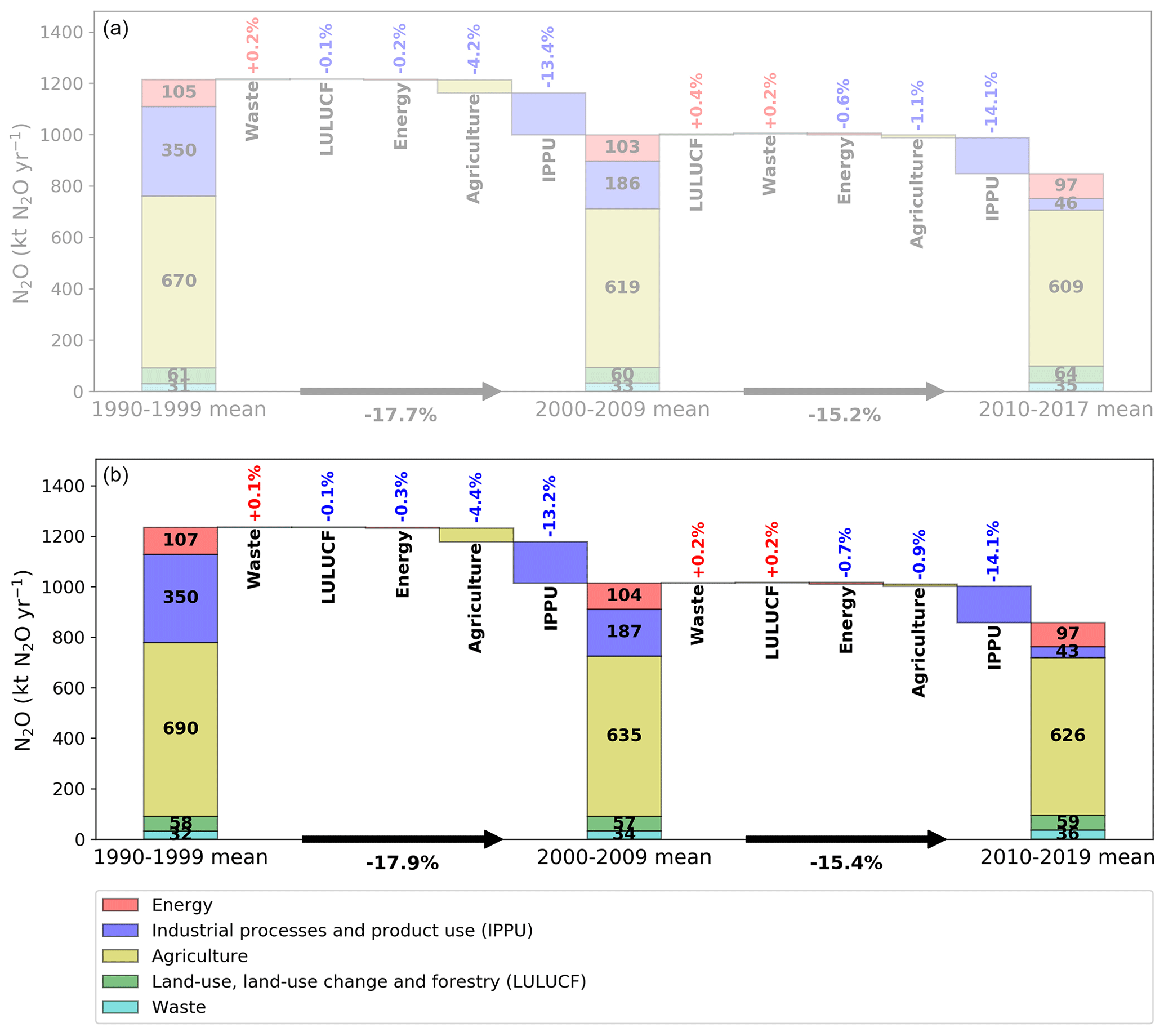
Figure 11 The contribution of changes (%) in N₂O anthropogenic emissions in the five sectors to the overall change in decadal mean for the EU27 + UK as reported to UNFCCC. Panel (a) shows the previous NGHGI data in Petrescu et al. (2021), and panel (b) depicts data from UNFCCC NGHGI (2021). The three stacked columns represent the average N₂O emissions from each sector during three periods (1990–1999, 2000–2009 and 2010–2019), and percentages represent the contribution of each sector to the total reduction percentages between periods.

3.2.3 NGHGI estimates compared with bottom-up inventories

Figure 12 compares the six bottom-up inventories with UNFCCC NGHGI (2021) data and shows that all of them are around the NGHGI estimates (Fig. 12a), noting that GAINS only provides emissions every 5 years. The BU estimates show good agreement with one another and with the NGHGI estimates until 2005. After 2005 the slightly increasing trend is influenced by the IPPU (Fig. 12c) and waste (Fig. 12e) sectors, with estimates of both EDGARv6.0 and GAINS for total anthropogenic N₂O emissions in the year 2018 being 9 % and 13 % higher than the respective UNFCCC NGHGI (2021) estimates. Except for agriculture (Fig. 12d), where four of the five models/inventories show a good match in absolute mean values with the NGHGI and over 1990–2018 and have similar linear trends of −0.18, −0.17, −0.15 and −0.11 % yr⁻¹ in NGHGI, EDGARv6.0, GAINS and FAOSTAT, respectively; for the other sectors the trends differ. The match in agriculture trends reflects that the sources rely on the same basic activity data from FAOSTAT and follow the IPCC EF Tier 1 or 2 approach (Petrescu et al., 2020). However, the high reported uncertainty range from the NGHGIs contradicts the match of the BU estimate absolute values and represents an important research question to be further investigated. In contrast, ECOSSE shows lower estimates because it does not use the FAO fertilizer application rate database but instead calculates ideal fertilizer application rates from the nitrogen demand of the crops. ECOSSE uses fertilizer data derived by Mueller et al. (2012) and simulates only for winter wheat. It is very likely that the assumed fertilizer application rates are lower than those used in FAO for the country-specific average, which could explain the lower estimates. This means that it may severely underestimate the applied fertilizer amounts for some areas (e.g., the Netherlands, Denmark or northwestern Germany), and the results are more indicative of emissions under idealized fertilizer application rates. Additionally, as mentioned above, the model simulates only the direct emissions.

Figure 12 (a) Total annual anthropogenic N₂O emissions (excluding LULUCF) for the EU27 + UK over time. The top plot presents previous data synthesized in Petrescu et al. (2021), while the bottom plot depicts data synthesized by the current study: (a) EU27 + UK and total sectoral emissions from (b) energy, (c) IPPU, (d) agriculture, and (e) waste from UNFCCC NGHGI (2021) submissions compared to global BU inventories for agriculture (CAPRI, ECOSSE, FAOSTAT, DayCent) and all sectors excluding LULUCF (EDGARv6.0, GAINS). CAPRI reports one value for Belgium and Luxembourg. The relative error on the UNFCCC value represents the UNFCCC NGHGI (2021) member-state-reported uncertainties computed with the error propagation method (95 % confidence interval) that were gap-filled and provided for every year. The uncertainty for EDGARv6.0 is the same as that of v5.0 and calculated for 2015 as min/max values for the total and each sector (Solazzo et al., 2021) and represents the 95 % confidence interval of a lognormal distribution. CAPRI reports uncertainties for the last 3 years as follows: 2014 and 2016 (17.6 %) and 2018 (17.8 %). The mean column represents the common overlapping period of 1990–2018 between datasets. The last years of the time series of the respective datasets are 2019 (UNFCCC and FAOSTAT), 2018 (EDGARv6.0, CAPRI), 2015 (GAINS every 5 years), 2015–2019 (DayCent) and 2020 ECOSSE, with the last 2 years reporting only crop emissions.

In the NGHGI (2021) submissions, for 2019, the EU27 + UK Tier 1 total uncertainty for the waste sector (based on the IPCC chap. 3 error propagation method described in detail by Petrescu et al., 2020) and the gap-filling method described in Appendix A was 360 %. The sectoral activity responsible for this high uncertainty is the wastewater treatment and discharge (462 %), and this remains one of the most uncertain sources of N₂O having the highest emissions in the waste sector. Emissions are known to vary markedly in space and time even within a single wastewater treatment plant (Gruber et al., 2020), a fact that only recently has been properly accounted for in the inventory guidelines (IPCC, 2019). However, the total emissions from the waste sector account for only 4.2 % of the total EU27 + UK 2019 N₂O emissions (excluding LULUCF).

3.2.4 NGHGI estimates compared to atmospheric inversions

Figure 13 compares inversion estimates of total N₂O emissions, including natural, from regional (FLEXINVERT) and global (three models) N₂O inversions with the UNFCCC NGHGI (2021) estimates. The min–max range of all inversions is within the 2σ uncertainty of NGHGI, with the median of global inversions being on average 42 % or 0.4 Tg N₂O yr⁻¹ higher than that of NGHGI. Over the period of 2005–2019, the regional FLEXINVERT is almost double that of UNFCCC NGHGI (2021). From the three global inversions, MIROC4-ACTM shows consistently higher estimates until 2019, when it registers a drop in the estimated emission level (similar to FLEXINVERT). A similar reduction of emissions is seen for 2003 and 2005. In all these years, Europe registered record-breaking heat waves. One plausible explanation for the low N₂O is that high temperature accompanied with lesser soil moisture reduces N₂O emission, as seen in the tropics (Patra et al., 2022).

The other two global inverse models, TOMCAT and CAMS-N₂O, register high estimates as well as very high variability. Regarding trends, FLEXINVERT shows a similar decreasing trend of 18 % over 2005–2019, compared to 16 % for UNFCCC NGHGI (2021). The global CAMS-N₂O inversion agrees the best in its absolute mean value (1.0 Tg N₂O yr⁻¹) with the NGHGI estimate (0.9 Tg N₂O yr⁻¹) but not in its trend. In this updated synthesis, natural pre-industrial soil emissions of N₂O from the O-CN model were included, but these are not considered in NGHGI reporting and therefore cannot explain the gap between inventories and TD estimates. In addition, the emission factors used in NGHGI reporting are regarded to be very uncertain (up to 300 % for direct agricultural emissions), which, based on the comparison with TD estimates, could imply that inventories underestimate N₂O emissions. The uncertainty reported by the NGHGIs in 2019 was 59 % compared to 86 % in 2017 (Petrescu et al., 2021).

Regarding the natural N₂O emissions, the median natural flux from inland waters (RECCAP2 estimate, Appendix A3) is very low (12.7 kt N₂O yr⁻¹), and part of the inland water natural estimate is considered anthropogenic in Europe and is due to the leaching of N fertilizers from agriculture. The anthropogenic share accounts for 66 % of the total inland waters emissions (Petrescu et al., 2021). In the current study more natural N₂O estimates have been added. The soil natural background emissions are estimated at 177 kt N₂O yr⁻¹ averaged over 2005–2014 (the common overlapping period of all data sources), while the biomass burning emissions account for only 1.6 kt N₂O yr⁻¹ for the same period. In the lower plot, the NGHGI uncertainty was recalculated to 56 % compared to 86 % in Petrescu et al. (2021) (upper plot).

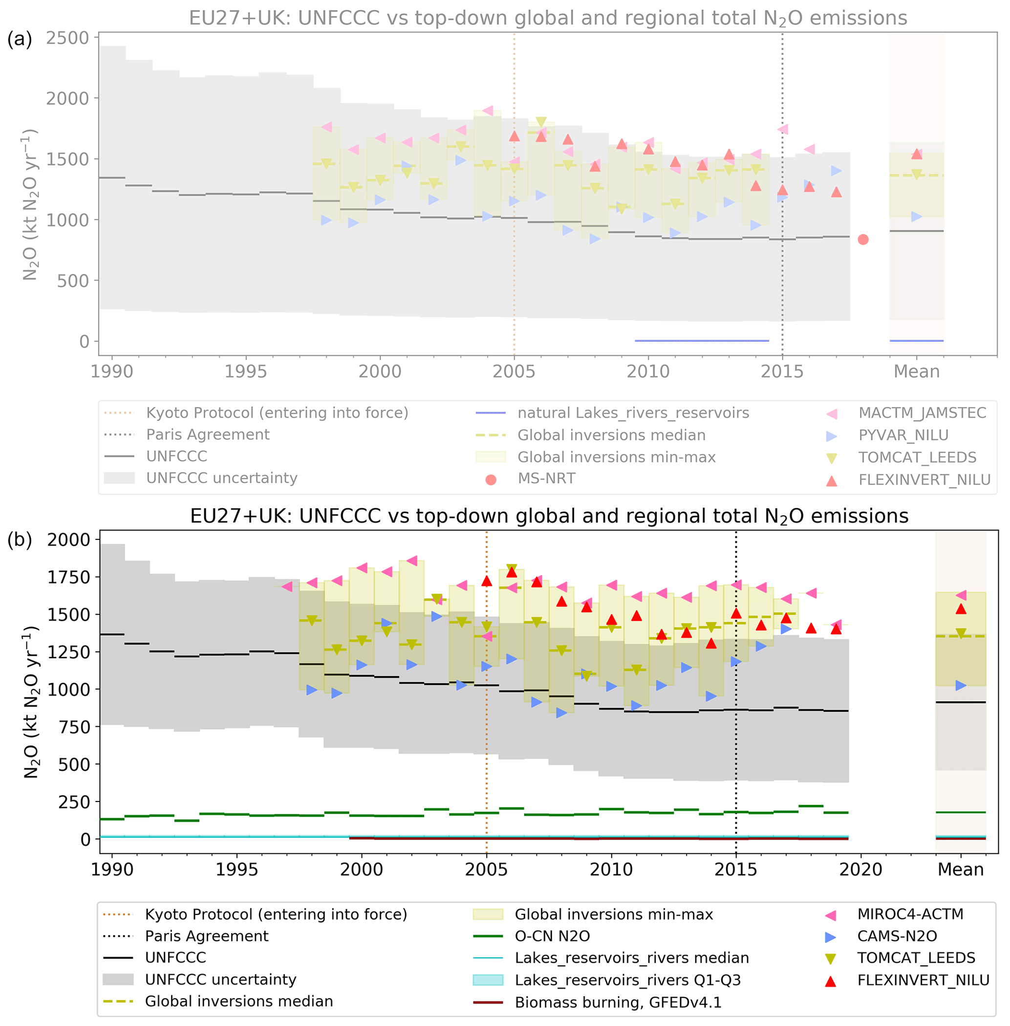
Figure 13 Comparison of total N₂O emissions for the EU27 + UK from one top-down regional inversion (FLEXINVERT) and three inversions (TOMCAT, CAMS-N₂O and MIROC4-ACTM) with UNFCCC NGHGI (gray) data and natural N₂O emissions (lakes, reservoirs and rivers from RECCAP2; natural pre-industrial soil emissions from the O-CN model; and biomass burning from GFEDv4.1) as follows: panel (a) shows the previous synthesized data in Petrescu et al. (2021), and panel (b) depicts data synthesized by the current study. The relative error on the UNFCCC value represents the UNFCCC NGHGI (2021) member-state-reported uncertainties computed with the error propagation method (95 % confidence interval) that were gap-filled and provided for every year (including LULUCF). The last years of the time series of the respective datasets are 2014 (TOMCAT), 2017 (CAMS-N₂O) and 2019 (UNFCCC, FLEXINVERT and MIROC4-ACTM). The mean column represents the common overlapping period (2005–2014) between datasets; MACTM-JAMSTEC and PYVAR_NILU in panel (a) are the same as MIROC4-ACTM and CAMS-N₂O in panel (b).

For the N₂O results (FLEXINVERT in Fig. 13), after updating the last runs, both the magnitude and trends of the N₂O emissions changed. This new decreasing trend confirms the UNFCCC trend but shows a larger average source after correcting for the estimate of natural emissions. Future work should strongly focus on establishing the uncertainty and variability in the natural emissions of N₂O so that the results of inversion could be more directly compared to emission inventories.

Spatial distribution of N₂O emissions from regional inversions

New top-down estimates of N₂O fluxes were produced using the CIF (Berchet et al., 2021). For N₂O, inversions were performed by LSCE using three CHIMERE setups and by NILU using FLEXPART(v10.4). For the CIF inversions, the prior fluxes and observations of N₂O were the same as those used in Fig. 13, and the background mixing ratios were calculated using the CAMSv19r products for N₂O (Segers, 2020), based on the global TM5-4DVAR assimilation run (Bergamaschi et al., 2018b, Rödenbeck et al., 2009).

For N₂O, the FLEXPART inversion resulted in slightly larger fluxes over Europe compared to the CHIMERE inversion, especially over the Netherlands, Belgium, northern France and England. In these regions, FLEXPART also results in larger fluxes compared to the prior. FLEXPART estimated smaller fluxes compared to the prior and to CHIMERE in northeastern Germany. CHIMERE, on the other hand, remained close to the prior estimates. The total mean emission for the EU27 + UK for the period of 2005–2018 was 1538 kt N₂O and 1680 kt N₂O yr⁻¹ for CHIMERE and FLEXPART, respectively, compared to the estimate of 1513 kt N₂O yr⁻¹ from FLEXPART (Fig. 13). Both inversions also found a decreasing trend over 2005–2018, with decreases of 157 and 298 kt N₂O yr⁻¹ for CHIMERE and FLEXPART, respectively, which was not seen in the prior estimates.

Figure 14 Posterior N₂O fluxes averaged over 2005–2018 (g N₂O m⁻² yr⁻¹) from two regional inversions, CHIMERE (LSCE) and FLEXPART (NILU), shown with a log-base-2 color scale (top) and the flux increments (posterior − prior) (g N₂O m⁻² yr⁻¹) shown on a linear color scale.

Similar to CH₄, the differences might be owing to the different dataset used for determining the background mixing ratios. Further analysis is ongoing.

4 Data availability

Data files reported in this work which were used for calculations and figures are available for public download at https://doi.org/10.5281/zenodo.7553800 (Petrescu et al., 2023). The data are reachable with one click (without the need for entering login and password) and can be downloaded with a second click, consistent with the two-click-access principle for data published in ESSD (Carlson and Oda, 2018). The data and the DOI number are subject to future updates and only refer to this version of the paper. The raw gridded data, according to the VERIFY consortium governing document, will be made publicly available 12 months after its publication in ESSD.

5 Summary and concluding remarks

This study is an update of the first comprehensive synthesis of European CH₄ and N₂O emission estimates (Petrescu et al., 2021), which compares total and sectoral European CH₄ and N₂O from BU (anthropogenic and natural) with TD estimates to assess their use for quality control and verification of UNFCCC NGHGI reporting. Using the most recent data, differences between TD and BU estimates were compared, and comparisons were made with the previous synthesis, Petrescu et al. (2021). Identification of source-specific uncertainty is key in understanding these differences and can lead to a reduction of the overall uncertainty in GHG inventories. Furthermore, the results have been synthesized in a way that would be compatible with the methodological framework of the first 2023 GST of the Paris Agreement. Five-year means of CH₄ (Fig. 1) and N₂O (Fig. 10) emissions for the periods 2011–2015 and 2015–2019 from the different BU and TD datasets have been calculated for the EU27 + UK bloc, as well as for five regions in Europe. These estimates are then compared with respective NGHGI emissions for the same periods and the 1990 base year.

Inconsistencies between CH₄ BU estimates and NGHGI data at the EU27 + UK level (Fig. 3) are mainly caused by different methodologies in calculating emissions as highlighted in Petrescu et al. (2020, 2021). Both BU inventories and the NGHGI use similar activity data and, to varying extents, the default EFs reported in the IPCC (2006) guidelines, meaning that the estimates are predestinated to agree rather well. Thus, the spread in all BU estimates may not be indicative of the uncertainty. For global consistency purposes, EDGARv6.0 and FAOSTAT mostly use Tier 1 approaches in calculating emissions (and uncertainties), a fact which triggers differences with other data sources using Tier 2 or 3 methods (GAINS for all sectors and CAPRI for agriculture). Within the UNFCCC reporting process, the agriculture sector was the highest contributor to the CH₄ emissions, followed by energy and waste (Fig. 1).

A reason for the small inconsistencies between datasets is the allocation of emissions to different sectors and that some data sources use updated methods and emission factors from different versions of the IPCC guidelines (e.g., 1996 versus 2006 or 2019 refinements to the 2006 IPCC guidelines, i.e., EDGARv6.0).

For N₂O anthropogenic emissions, all BU data sources show good agreement with the UNFCCC NGHGI (2021) data in both trends and means (Fig. 12), with agriculture remaining the largest emitter (e.g., soil emissions due to fertilizer additions), within the reported uncertainties. As with CH₄, the different BU estimates share some common elements such as activity data and emissions factors, and the agreement between estimates may not be relevant to the underlying uncertainties.

An important improvement compared to Petrescu et al. (2021) was the harmonization of UNFCCC member state uncertainty estimates, which were gap-filled and calculated for each year of the time series. VERIFY interaction with the EU inventory team has helped improve the uncertainty estimations on the EU GHG emissions reported under UNFCCC. For both CH₄ and N₂O the uncertainties reported by NGHGI are large and underline the need for further improvement in the inventories of these two GHGs.

Regarding the TD estimates, this analysis shows that comparison between CH₄ inversion estimates and NGHGIs is highly uncertain because of the large spread in the inversion results. Nevertheless, in contrast to BU methods, TD inversions inferred from atmospheric observations represent the most independent data against which CH₄ inventory totals can be compared. With anticipated improvements in atmospheric modeling and observations, as well as modeling of natural fluxes, TD inversions may arguably emerge as the most powerful tool for verifying emission inventories for CH₄ and other GHGs.

As TD inversions do not fully distinguish between all emission sectors used by NGHGI and report either total emissions or a coarse sectorial partitioning, their comparison to NGHGI is only possible for total emissions. It is also necessary to make an adjustment for natural emissions, which are included in TD inversions but not reported by the NGHGIs. A future improvement for the natural CH₄ emissions is the consistent time series of measurements to make clear statements about how wetland and lake fluxes change over time. For lakes there is virtually no long-term monitoring, while for wetlands variability (e.g., area) is a key uncertainty, but Fronzek et al. (2018) have shown that model ensembles work well in simulating highly uncertain variables. In general, regional inversions show less spread than the global inversions as they used recent updates of transport models and simulate atmospheric transport at higher resolutions.

The global models use fewer observations for Europe compared to the included regional inversions and thus are expected to have larger uncertainties for the European fluxes. In addition, the global models are at coarser resolution and thus likely have larger model representation errors compared to the regional ones, which may contribute to further systematic uncertainty for the European fluxes. Currently, for Europe the regional TD total is considerably higher than the global estimates (Fig. 1). If the regional TD estimate for the whole EU27 + UK including all sources and sinks is considered to be the best total estimate in place and if the natural fluxes are assumed to have been accurately subtracted from the optimized net flux, then NGHGI and BU approaches may be underestimating total EU27 + UK CH₄ emissions by approximately 20 %–30 %. For N₂O, the TD estimates fall within the large range of the NGHGI uncertainties, and, in fact, the spread in the regional ensembles is much smaller than the inventory uncertainty range (Fig. 13). Compared to Petrescu et al. (2021), the natural emissions consisting of pre-industrial natural soil emissions and biomass burning emissions were included; however, for N₂O natural emissions do not explain the 415 kt N₂O difference between NGHGI (and BU) estimates and the average TD estimate. More research is thus needed to identify the source of discrepancies.

A key challenge for the inversion CH₄ community remains the separation of emissions in specific source sectors, as derived total emissions may also include natural emissions (or removals). In the case of N₂O this will not be possible since the anthropogenic emissions due to agriculture are caused by a perturbation to microbial processes (i.e., nitrification and denitrification) and cannot be cleanly separated from natural emissions (defined as the level of emission in the pre-industrial period, i.e., before perturbation by anthropogenic N inputs). However, some TD quantification of industrial emissions should be possible in high-resolution inversions. In any case, TD inversions for estimating N₂O emissions should mainly focus on the trends. Furthermore, the accuracy of derived emissions and the spatial scales at which emissions can be estimated depend on the quality and density of measurements and the quality of the atmospheric models (Bergamaschi et al., 2018a). Significant further developments of the global observations system and the top-down methods would be required to support the implementation of the Paris Agreement.

The exercise of presenting uncertainty reduction maps illustrated the effect on uncertainty reductions with removing/adding ground-based observation stations. This is one of the elements informing policy makers on the need for further investing into a denser and efficient surface observation network used by inverse systems to calibrate their estimates and better inform climate policy with respect to emission verification. This might serve to monitor and build a more accurate budget of country estimates as well as provide data for inferring subnational (e.g., city-scale) emissions.

This synthesis makes use and brings together state-of-the-art BU and TD estimates from different sources and compares these data with the official NGHGI estimates reported to UNFCCC. The exercise underlines the uncertainties in the emissions of these important GHGs and illustrates the importance of regional consistent analyses and synthesis of available estimates for informing climate policy. Specifically, the approach demonstrated here could form the basis of the multilateral facilitative consideration of progress under the enhanced transparency framework of the Paris Agreement. The implementation of the Paris Agreement requires accurate quantification of GHG emissions in order to track the progress of all parties with their nationally determined contributions and to assess collective progress towards achieving the purpose of this agreement and its long-term goals (GST). As this will be mainly achieved and built upon BU methodologies developed by the IPCC, we need to take into consideration the potential to quantify GHG emissions by using top-down methods (inverse modeling) (Bergamaschi et al., 2018a). One advantage of the inverse estimate is that it provides total emission estimates inferred from atmospheric GHG measurements. Therefore, the capability to quantify anthropogenic emissions depends on the magnitude of natural sources and sinks and the capability to quantify them and subtract them from the TD estimates.

As stated in the introduction, the main aim was to explore and discuss the issues causing differences between NGHGI, BU and TD approaches. Such an exercise can help to improve the different respective approaches and furthermore can inform the development of formal verification systems. Some differences in BU and NGHGI estimates were observed and were traced back to factors such as the variation activity data, emission factors and sectoral allocation of emissions (CH₄). Nevertheless, BU and NGHGI estimates generally converged at the total emission level for the EU27 + UK bloc and the five European regions. The overall agreement is generally due to similar sources of input activity data and emission factors (albeit with some aforementioned variations) and is not indicative of the true uncertainties in the respective CH₄ and N₂O inventories. Indeed, NGHGIs report CH₄ and N₂O emissions with large uncertainties, and, furthermore, NGHGI estimates generally diverged from the respective TD fluxes. Despite the significant spread in the inversion estimates (due to, e.g., use of different transport models and/or observation datasets, while priors might be the same; Table B4), TD estimates were generally higher than NGHGI, even when accounting for the (albeit uncertain) natural fluxes.

The analysis done here generally compared estimates in terms of long-term trends and averages over 5 or more years and thus provides a working example of how such syntheses could inform future GSTs under the Paris Agreement. A further step could involve analysis at finer temporal resolutions. While NGHGIs are reported at annual scales, analyzing emissions over intra-annual timescales, of great importance for CH₄ (wetland emission estimates have large uncertainties and show large variability in space and between seasons) and N₂O (agricultural fertilizer application), may help to identify sector contributions to divergence between prior and posterior estimates at the annual and/or inter-annual scale. To o this, however, requires expanded in situ monitoring so that such dynamics can be better represented in the temporally resolved prior estimates that feed into the top-down inversions.

Appendix A: Data sources, methodology and uncertainty descriptions

The country-specific plots are found at http://webportals.ipsl.jussieu.fr/VERIFY/FactSheets/v1.28 (last access: January 2023).

VERIFY project

VERIFY's primary aim was to develop scientifically robust methods to assess the accuracy and potential biases in national inventories reported by the parties through an independent pre-operational framework. The main concept is to provide observation-based estimates of anthropogenic and natural GHG emissions and sinks as well as associated uncertainties. The proposed approach is based on the integration of atmospheric measurements, improved emission inventories, ecosystem data, and satellite observations and on an understanding of processes controlling GHG fluxes (ecosystem models, GHG emission models).

Two complementary approaches relying on observational data streams were combined in VERIFY to quantify GHG fluxes:

1. atmospheric GHG concentrations from satellites and ground-based networks (top-down atmospheric inversion models) and

2. bottom-up activity data (e.g., fuel use and emission factors) and ecosystem measurements (bottom-up models).

For CH₄ and N₂O, agricultural emissions were separated from fossil fuel and industrial emissions. Finally, trends in the budget of the three GHGs were analyzed in the context of NDC targets.

The objectives of VERIFY were the following.

Objective 1. Integrate the efforts between the research community, national inventory compilers, operational centers in Europe and international organizations towards the definition of future international standards for the verification of GHG emissions and sinks based on independent observation.

Objective 2. Enhance the current observation and modeling ability to accurately and transparently quantify the sinks and sources of GHGs in the land use sector for the tracking of land-based mitigation activities.

Objective 3. Develop new research approaches to monitor anthropogenic GHG emissions in support of the EU commitment to reduce its GHG emissions by 40 % by 2030 compared to the year 1990.

Objective 4. Produce periodic scientific syntheses of observation-based GHG balance of EU countries and practical policy-oriented assessments of GHG emission trends, and apply these methodologies to other countries.

For more information on the project team and products/results check https://verify.lsce.ipsl.fr/ (last access: January 2023).

Table A1 Country grouping used for reconciliation purposes between BU and TD estimates. The countries and groups of countries in italic are not directly used by this study, but their figures and data are available on the VERIFY project web portal at http://webportals.ipsl.jussieu.fr/VERIFY/FactSheets/ (last access: January 2023).

Countries highlighted in italic are not discussed in the current synthesis mostly because of unavailability of NGHGI data (non-Annex I countries are mostly developing countries; the reporting to UNFCCC is implemented through national communications (NCs) and biennial update reports (BURs): https://unfccc.int/national-reports-from-non-annex-i-parties., last access: January 2023) but are present on the web portal: http://webportals.ipsl.jussieu.fr/VERIFY/FactSheets/ (last access: January 2023). Results of Annex I countries (NOR, CHE, ISL) and non-EU EAE countries/groups are represented in Figs. 1 and 9.

Table A2 Main methodological changes (in bold) of the current study with respect to Petrescu et al. (2020, 2021); NA cells mean that there are no data available.

A1 Anthropogenic CH₄ emissions (sectors energy, IPPU, agriculture, LULUCF and waste)

A1.1 Bottom-up CH₄ emission estimates

UNFCCC NGHGI (2021)

Under the UNFCCC and its Kyoto Protocol national greenhouse gas (GHG) inventories are the most important source of information to track progress and assess climate protection measures by countries. In order to build mutual trust in the reliability of the GHG emission information provided, national GHG inventories are subject to standardized reporting requirements, which have been continuously developed by the Conference of the Parties (COP)⁷. The calculation methods for the estimation of greenhouse gases in the respective sectors is determined by the methods provided by the 2006 IPCC Guidelines for National Greenhouse Gas Inventories (IPCC, 2006). These guidelines provide detailed methodological descriptions to estimate emissions and removals, as well as provide recommendations to collect the activity data needed. As a general overall requirement, the UNFCCC reporting guidelines stipulate that reporting under the Convention and the Kyoto Protocol follows the five key principles of transparency, accuracy, completeness, consistency and comparability (TACCC).

The reporting under UNFCCC should meet the TACCC principles. The three main GHGs are reported in time series from 1990 up to 2 years before the due date of the reporting. The reporting is strictly source category based and is done under the common reporting format (CRF) tables, downloadable from the UNFCCC official submission portal: https://unfccc.int/ghg-inventories-annex-i-parties/2021 (last access: March 2022).

The UNFCCC NGHGI anthropogenic CH₄ and N₂O emissions analyzed in this study include estimates from four key sectors for the EU27 + UK: (1) energy, (2) industrial processes and product use (IPPU), (3) agriculture, and (5) waste. The methodological tiers a country applies depends on the source contribution to the national total (key category or not), on the national circumstances and on the individual conditions of the land, which explains the variability of uncertainties among the sector itself as well as among EU countries. The LULUCF CH₄ and N₂O emissions are very small but are included in some figures (see Table 1).

Gap-filling harmonization procedure for NGHGI uncertainties

The presented uncertainties in the emission levels of the individual countries and the EU27 + UK bloc were calculated by using the methods and data used to compile the official GHG emission uncertainties that are reported by the EU under the UNFCCC NIRs (UNFCCC NGHGI, 2022). The EU uncertainty analysis reported in the bloc's National Inventory Report (NIR) is based on country-level, Approach 1 uncertainty estimates (IPCC, 2006, vol. 1, chap. 3) that are reported by EU member states, Iceland and the United Kingdom under Article 7(1)(p) of Regulation (EU) 525/2013 (2020). These country-level uncertainty estimates are typically reported at the beginning of a submission cycle and are not always revised with updated CRF submissions later in the submission cycle. Furthermore, the compiled uncertainties of some countries are incomplete (e.g., uncertainties not estimated for LULUCF and/or indirect CO₂ emissions, certain subsector emissions are confidential), and the sector and gas resolution at which uncertainties are provided varies between the countries. The EU inventory team therefore implements a procedure to harmonize and gap-fill these uncertainty estimates. A processing routine reads the individual country uncertainty files that are pre-formatted manually to assign consistent sector and gas labels to the respective estimates of emissions/removals and uncertainties. The uncertainty values are then aggregated to a common sector resolution, at which the emissions and removals reported in the uncertainty tables of the countries are then replaced with the respective values from the final CRF tables of the countries. Due to the issue of incompleteness mentioned above, the country-level data are then screened to identify residual GHG emissions and removals for which no uncertainty estimates have been provided. Where sectors are partially complete, the residual net emission is quantified in CO₂ equivalents and incorporated. An uncertainty is then estimated by calculating the overall sector uncertainty of the sources and sinks that were included in that country's reported uncertainty estimates and assigning this percentage average to the residual net emission. In cases where for certain sectors no uncertainties have been provided at all (e.g., indirect CO₂ emissions, LULUCF), an average (median) sector uncertainty in percent is calculated from all the countries for which complete sectoral emissions and uncertainties were reported, and this average uncertainty is assigned to the country's sector GHG total reported in its final CRF tables.

The country-level uncertainties presented in this paper were provided by the EU GHG inventory team and have been compiled using this same processing routine and using the uncertainties and CRF data reported by the countries in the 2021 submission. However, for the purpose of this synthesis work, the method has been expanded to gap-fill at the individual greenhouse gas level (CH₄ and N₂O emissions only) rather than at the aggregate GHG level. Furthermore, the expanded method here assigns the sub-sectoral uncertainties to the emissions and removals of the entire time series (1990–2019) rather than just the base year and latest year of the respective time series. This allows uncertainties to be sensitive to the sub-sectoral contributions to sectoral and national total emissions, which of course change over time. For each year of the time series, uncertainties in the total and sectoral CH₄ and N₂O emissions are calculated using Gaussian error propagation, by summing the respective sub-sectoral uncertainties (expressed in kilotons CH₄ and N₂O) in quadrature and assuming no error correlation. In contrast, for the EU27 + UK bloc, uncertainties in the total and sectoral CH₄ and N₂O emissions were calculated to take into account error correlations between the respective country estimates at the subsector level. This was done by applying the same methods and assumptions described in the 2022 EU NIR (UNFCCC NGHGI, 2022). The subsector resolution applied for gap-filling allows the routine to access respective data on emission factors from CRF Table “Summary 3” (UNFCCC NGHGI, 2021) and apply correlation coefficients (r) when aggregating the uncertainties. For a given subsector, it is assumed that the errors of countries using default factors are completely correlated (r=1), while errors of countries using country-specific factors are assumed uncorrelated (r=0). For countries using a mix of default and country-specific factors at the given subsector level, it is assumed that these errors are partially correlated (r=0.5) with one another and with the errors of countries using the default factors only.

Based on these correlation assumptions, the routine then aggregates CH₄ and N₂O emissions and uncertainties for the specified subsector resolution at the EU27 + UK level. Uncertainties at the total sector level are then aggregated from the subsector estimates assuming no correlation between subsectors. However, for countries reporting very coarse resolution estimates (e.g., total sector CH₄ and N₂O emissions) or where the sector has been partially or completely gap-filled, it is assumed that these uncertainties are partially correlated (r=0.5) with one another and with the other reported subsector level estimates. Level uncertainties on the total EU27 + UK CH₄ and N₂O emissions (with and without LULUCF) are then aggregated from the sector estimates assuming no error correlation between sectors.

EDGARv6.0

The Emissions Database for Global Atmospheric Research (EDGAR) is an independent global emission inventory of greenhouse gases (GHG) and air pollutants developed by the Joint Research Centre of the European Commission (https://edgar.jrc.ec.europa.eu/index.php, last access: May 2022). The first edition of the Emissions Database for Global Atmospheric Research was published in 1995. The dataset now includes almost all sources of fossil CO₂ emissions, is updated annually, and reports data for 1970 to n−1. Estimates are provided by sector. Emissions are estimated fully based on statistical data from 1970 until 2018 (https://data.jrc.ec.europa.eu/dataset/97a67d67-c62e-4826-b873-9d972c4f670b, last access: November 2022). For complete description see Andrew (2020).

Uncertainties. EDGAR uses emission factors (EFs) and activity data (AD) to estimate emissions. Both EFs and AD are uncertain to some degree, and when combined, their uncertainties need to be combined too. To estimate EDGAR's uncertainties (stemming from a lack of knowledge of the true value of the EF and AD), the methodology devised by IPCC (2006, chap. 3) is adopted, that is, the sum of squares of the uncertainty of the EF and AD (uncertainty of the product of two variables). A lognormal probability distribution function is assumed to avoid negative values, and uncertainties are reported as 95 % confidence intervals according to IPCC (2006, chap. 3, Eq. 3.7). For emission uncertainty in the range 50 % to 230 % a correction factor is adopted as suggested by Frey et al. (2003) and IPCC (2006, chap. 3, Eq. 3.4). Uncertainties are published in Solazzo et al. (2021).

CAPRI

CAPRI is an economic, partial equilibrium model for the agricultural sector, focused on the EU (Britz and Witzke, 2014⁸; Weiss and Leip, 2012⁹). CAPRI stands for Common Agricultural Policy Regional Impact Analysis, and the name hints at the main objective of the system: assessing the effect of CAP policy instruments not only at the EU or member state level but at sub-national level too. The model is calibrated for the base year (currently 2012), and then baseline projections are built, allowing the ex ante evaluation of agricultural policies and trade policies on production, income, markets, trade and the environment.

Among other environmental indicators, CAPRI simulates CH₄ emissions from agricultural production activities (enteric fermentation, manure management, rice cultivation, agricultural soils). Activity data are mainly based on FAOSTAT and EUROSTAT statistics, and estimation of emissions follows IPCC (2006) methodologies, with a higher or lower level of detail depending on the importance of the emission source. Details on CAPRI methodology for emission calculations is referenced in Table A1. For this study CAPRI updated emissions for 3 years: 2014, 2016 and 2018.

Uncertainties were calculated for the updated years, 2014, 2016 and 2018. The uncertainty of the spatial allocation of emissions for CH₄ and N₂O has been calculated by taking into account the uncertainty of the spatial disaggregation and the uncertainty of the emission sources, assuming

• the disaggregation has an uncertainty of 50 % for N₂O and 20 % for CH₄ and

• the emission processes have an uncertainty of

• –

  50 %: N₂O soil processes,

• –

  30 %: N₂O manure processes,

• –

  30 %: CH₄ manure and enteric, and

• –

  10 %: rice.

Then, for each cell, the uncertainty of the disaggregation and that of the process are combined as they are independent (sum of squares; see Solazzo et al., 2021), and then the total uncertainty for the grid cell is aggregated using emission weighted sum of squares.

GAINS

Specific sectors and abatement technologies in GAINS vary by the specific emitted compound, with source sector definition and emission factors largely following the IPCC methodology at the Tier 1 or Tier 2 level. GAINS includes in general all anthropogenic emissions to air but does not cover emissions from forest fires, savannah burning and land use/land use change. Emissions are estimated for 174 countries/regions, with the possibility to aggregate to a global emission estimate, and spanning a time frame from 1990 to 2050 in 5-year intervals. Activity drivers for macroeconomic development, energy supply and demand, and agricultural activities are entered externally; GAINS extends with knowledge required to estimate “default” emissions (emissions occurring due to an economic activity without emission abatement) and emissions and costs of situations under emission control (see Amann et al., 2011).

The GAINS model covers all source sectors of anthropogenic methane (CH₄) emissions – agricultural sector emissions from livestock, rice cultivation and agricultural waste burning, energy sector emissions from upstream and downstream sources in fossil fuel extraction and use, and emissions from handling and treatment of solid waste and wastewater source sectors. A description of the modeling of CH₄ emissions in GAINS is presented in Höglund-Isaksson et al. (2020). Generation of solid waste and the carbon content of wastewater are derived within the model in consistency with the relevant macroeconomic scenario. The starting point for estimations of anthropogenic CH₄ is the methodology recommended in the IPCC (2006, and revision in 2019) guidelines, for most source sectors using country-specific information to allow for deriving country- and sector/technology-specific emission factors at a Tier 2 level. Consistent methodologies were further developed to estimate emissions from oil and gas systems (Höglund-Isaksson, 2017) and solid waste (Höglund-Isaksson et al., 2018; Gómez-Sanabria et al., 2018). Emission factors are specified in a consistent manner across countries for given sets of technology and with past implementation of emission abatement measures reflected as changes in technology structures. The resulting emission estimates are well comparable across geographic and temporal scales. The GAINS approach to calculate waste emissions is developed in consistency with the first-order-decay method recommended by IPCC (2006 and 2019 revision), applying different decay periods when estimating emissions from flows of different types of organic waste, i.e., food and garden, paper, wood, textile, and other. Data on waste generation, composition and treatment are taken from EUROSTAT (2019) and complemented with national information from the UNFCCC NGHGI (2019) common reporting format tables on the amounts of waste diverted to landfills of various management levels and to treatment, e.g., recycling, composting, biodigestion and incineration.

Uncertainties. Uncertainty is prevalent among many different dimensions in the estimations of emissions, abatement potentials and costs. When constructing global bottom-up emission inventories at a detailed country and source level, it is inevitable that some information gaps will be bridged using default assumptions. As it is difficult to speculate about how such sources of uncertainty affect resulting historical and future emission estimates, we instead address uncertainty in historical emissions by making comparisons to estimates by other publicly available and independently developed bottom-up inventories and various top-down estimates consistent with atmospheric measurements and inverse model results. Although existing publicly available global bottom-up inventories adhere to the recommended guidelines of the IPCC (2006), the flexibility in these is large, and results will depend on the availability and quality of gathered source information. There is accordingly a wide range of possible sources of uncertainty built into estimations in such comprehensive efforts. Having a pool of independently developed inventories, each with its own strengths and weaknesses, can improve the understanding of the scope for uncertainty, in particular when compared against top-down atmospheric measurements.

FAOSTAT

The Food and Agriculture Organization of the United Nations (FAO) provides CH₄ emission totals per gas/activity from the agriculture and LULUCF sectors available at https://www.fao.org/faostat/en/#data/GT (last access: April 2022). The FAOSTAT emissions database is computed following Tier 1 of the 2006 IPCC Guidelines for National Greenhouse Gas Inventories (http://www.ipcc-nggip.iges.or.jp/public/2006gl/index.html, last access: January 2022). Country reports to FAO on crops, livestock and agriculture use of fertilizers are the source of activity data. Geospatial data are the source of AD for the estimates from cultivation of organic soils, biomass and peat fires. GHG emissions are provided by country, regions and special groups, with global coverage, relative to the period of 1961–present (with annual updates, currently to 2019) and with projections for 2030 and 2050, expressed as CO₂ eq. for CH₄, by underlying agricultural emission sub-domain and by aggregate (agriculture total, agriculture total plus energy, agricultural soils). LULUCF emissions consist of CH₄ (methane) associated with biomass and peat fires. Comparison to the UNFCCC submissions is also provided.

Uncertainties were computed by Tubiello et al. (2013) but are not available in the FAOSTAT database.

A1.2 Top-down anthropogenic CH₄ emission estimates

FLEXPART – FLExKF

FLExKF applies an extended Kalman filter (Brunner et al., 2012) in combination with backward Lagrangian transport simulations using the model FLEXPART (Stohl et al., 2005; Pisso et al., 2019). It optimizes surface–atmosphere fluxes by assimilating atmospheric observations in a sequential manner, which allows for an analytical solution for relatively large inversion problems (long time periods, number stations O(100)). Since model–observation residuals typically follow a lognormal distribution, the method optimizes log-transformed emissions, which also guarantees a positive solution. Source–receptor matrices (Seibert and Frank, 2004) were computed at 0.25^∘ × 0.25^∘ resolution with FLEXPART driven by ECMWF ERA-Interim meteorological fields in the same way as for FLEXINVERT. Backward simulations were limited to 10 d prior to each observation and to the domain 30–75^∘ N, 15^∘ W–35^∘ E. Fluxes were estimated for this domain on a monthly basis at 0.5^∘ × 0.5^∘ resolution. For the version used in this study, FLExKF-CAMSv19r_EMPA, the background mole fraction was taken from CAMSv19r, which is based on the global TM5-4DVAR assimilation run (Bergamaschi et al., 2018b) where the above domain was cut out following the two-step approach of Rödenbeck et al. (2009).

Uncertainties. The uncertainty in the posterior fluxes is composed of random and systematic errors. The random uncertainties are represented by the posterior error covariance matrix provided by the Kalman filter, which combines errors in the prior fluxes with errors in the observations and model representation. Systematic uncertainties primarily arise from systematic errors in modeled atmospheric transport and in background mole fractions but also include aggregation errors, i.e., errors arising from the way the flux variables are discretized in space and time.

FLEXINVERT

The FLEXINVERT framework is based on Bayesian statistics and optimizes surface–atmosphere fluxes using the maximum probability solution (Rodgers, 2000). Atmospheric transport is modeled using the Lagrangian model FLEXPART (Stohl et al., 2005; Pisso et al., 2019) run in the backwards time mode to generate a so-called source–receptor matrix (SRM). The SRM describes the relationship between the change in mole fraction and the fluxes discretized in space and time (Seibert and Frank, 2004) and was calculated for 8 d prior to each observation. For use in the inversions, FLEXPART was driven using ECMWF operational analysis wind fields. The state vector consisted of prior fluxes discretized on an irregular grid based on the SRMs (Thompson et al., 2014). This grid has finer resolution (in this case the finest was 0.25^∘ × 0.25^∘) where the fluxes have a strong influence on the observations and coarser resolution where the influence is only weak (the coarsest was 2^∘ × 2^∘). The fluxes were solved at 10 d temporal resolution. The state vector also included scalars for the background contribution. The background mixing ratio, i.e., the contribution to the mixing ratio that is not accounted for in the 8 d SRMs, was estimated by coupling the termination points of backward trajectories (modeled using virtual particles) to initial fields of methane simulated with the Lagrangian FLEXPART-CTM model, which was developed at EMPA based on FLEXPART (Stohl et al., 2005; Pisso et al., 2019). The data assimilation method described by Groot Zwaaftink et al. (2018) that constrains modeled fields with surface observations through nudging was applied for current simulations.

Uncertainties. The posterior fluxes are subject to systematic errors primarily from (1) errors in the modeled atmospheric transport; (2) aggregation errors, i.e., errors arising from the way the flux variables are discretized in space and time; (3) errors in the background methane fields; and (4) the incomplete information from the observations and hence the dependence on the prior fluxes. In addition, there is, to a smaller extent, some error due to calibration offsets between observing instruments. Uncertainties in the observation space were inflated to take into account the model representation errors.

InGOS and TM5-4DVAR

The atmospheric models used within the European FP7 project InGOS (Integrated non-CO₂ Greenhouse gas Observing System) are described by Bergamaschi et al. (2018b) and their Supplement (https://doi.org/10.5194/acp-18-901-2018-supplement). The models include global Eulerian models with a zoom over Europe (TM5-4DVAR, TM5-CTE, LMDZ), regional Eulerian models (CHIMERE) and Lagrangian dispersion models (STILT, NAME, COMET). The horizontal resolutions over Europe are ∼1.0–1.2^∘ (longitude) $\times \sim \mathrm{0.8}$–1.0^∘ (latitude) for the global models (zoom) and ∼0.17–0.56^∘ (longitude) $\times \sim \mathrm{0.17}$–0.5^∘ (longitude) for the regional models. Most models are driven by meteorological fields from the European Centre for Medium-Range Weather Forecasts (ECMWF) ERA-Interim reanalysis (Dee et al., 2011). In the case of STILT, the operational ECMWF analyses were used, while for NAME meteorological analyses of the Met Office Unified Model (UM) were employed. The regional models use boundary conditions (background CH₄ mole fractions) from inversions of the global models (STILT from TM3, COMET from TM5-4DVAR, CHIMERE from LMDZ) or estimate the boundary conditions in the inversions (NAME) using baseline observations at Mace Head as prior estimates. In the case of NAME and CHIMERE, the boundary conditions are further optimized in the inversion. The inverse modeling systems applied in this study use different inversion techniques. TM5-4DVAR, LMDZ, and TM3-STILT use 4DVAR variational techniques, which allow optimization of emissions of individual grid cells. These 4DVAR techniques employ an adjoint model in order to iteratively minimize the cost function using a quasi-Newton (Gilbert and Lemaréchal, 1989) or conjugate gradient (Rödenbeck, 2005) algorithm. The NAME model applies a simulated annealing technique, a probabilistic technique for approximating the global minimum of the cost function. In CHIMERE and COMET, the inversions are performed analytically after reducing the number of parameters to be optimized by aggregating individual grid cells before the inversion. TM5-CTE applies an ensemble Kalman filter (EnKF) (Evensen, 2003), with a fixed-lag smoother (Peters et al., 2005).

Uncertainty. In general, the estimated model uncertainties depend on the type of station and for some models (TM5-4DVAR and NAME) also on the specific synoptic situation. In InGOS the uncertainty of the ensemble was calculated as 1σ estimate. Bergamaschi et al. (2015) showed that the range of the derived total CH₄ emissions from northwestern and eastern Europe using four different inverse modeling systems was considerably larger than the uncertainty estimates of the individual models because the latter typically use Bayes' theorem to calculate the reduction of assumed prior emission uncertainties by assimilating measurements (propagating estimated observation and model errors to the estimated emissions). An ensemble of inverse models may provide more realistic overall uncertainty estimates, since estimates of model errors are often based on strongly simplified assumptions and do not represent the total uncertainty.

InTEM – NAME

The Inverse Technique for Emission Modelling (InTEM) (Arnold et al., 2018) uses the NAME (Numerical Atmospheric dispersion Modelling Environment) (Jones et al., 2007) atmospheric Lagrangian transport model. NAME is driven by analysis 3D meteorology from the UK Met Office Unified Model (Cullen, 1993). The horizontal and vertical resolution of the meteorology has improved over the modeled period from 40 to 12 km (1.5 km over the UK). InTEM is a Bayesian system that minimizes the mismatch between the model and the atmospheric observations given the constraints imposed by the observation and model uncertainties and prior information with its associated uncertainties. The direction (latitude and longitude) and altitude varying background concentration and observation station bias are solved for within the inverse system along with the spatial distribution and magnitude of the emissions. The time-varying prior background concentration for the DECC network stations is derived from the MHD observations when they are very largely sensitive only to northern Canada (Arnold et al., 2018). The prior bias (which can be positive or negative) for each station is set to zero with an uncertainty of 1 ppb. The observations from each station are assumed to have an exponentially decreasing 12 h time correlation coefficient and, between stations, a 200 km spatial correlation coefficient. The observations are averaged into 2 h periods. The uncertainty of the observations is derived from the variability of the observations within each 2 h period. The modeling uncertainty for each 2 h period at each station varies and is defined as the larger of the median pollution events in that year at that station or 16.5 % of the magnitude of the pollution event. These values have been derived from analysis of the observations of methane at multiple heights at each station across the DECC network. Each inversion is repeated 24 times, each time 10 % of the observations per year per station are randomly removed in 5 d intervals, and the results and uncertainty are averaged.

Uncertainty. This random removal of observations allows a greater exploration of the uncertainty, given the potential for some of the emission sources to be intermittent within the time period of the inversion.

CTE-CH₄ Europe, CTE-SURF and CTE-GOSAT

CarbonTracker Europe CH₄ (CTE-CH₄) (Tsuruta et al., 2017) applies an ensemble Kalman filter (Peters et al., 2005) in combination with the Eulerian transport model TM5 (Krol et al., 2005). It optimizes surface fluxes weekly and assimilates atmospheric CH₄ observations. TM5 was run at 1^∘ × 1^∘ resolution over Europe and 6^∘ × 4^∘ resolution globally, constrained by 3-hourly ECMWF ERA-Interim meteorological data. The photochemical sink of CH₄ due to tropospheric and stratospheric OH as well as stratospheric Cl and O(¹D) was pre-calculated based on Houweling et al. (2014) and Brühl and Crutzen (1993) and not adjusted in the optimization scheme.

Three experiments were conducted, which differ in (1) sets of prior fluxes, (2) sets of assimilated observations and (3) optimization resolution over the Northern Hemisphere.

In the Petrescu et al. (2021) study, CTE-FMI used sets of prior fluxes from LPX-Bern DYPTOP (Stocker et al., 2014) for biospheric, EDGARv4.2 FT2010 (Janssens-Maenhout et al., 2013) for anthropogenic, GFEDv4 (Giglio et al., 2013) for biomass burning, Ito and Inatomi (2012) for termites, and Tsuruta et al. (2017) for ocean sources. CTE-SURF and CTE-GOSAT use sets of prior fluxes from Global Carbon Project (Saunois et al., 2020). CTE-FMI and CTE-SURF assimilated ground-based surface CH₄ observations, while CTE-GOSAT assimilated GOSAT XCH₄ retrievals from NIESv2.72. CTE-FMI optimized fluxes at 1^∘ × 1^∘ resolution over northern Europe, northeast Russia and southeast Canada; 6^∘ × 4^∘ resolution over other parts of the Northern Hemisphere land; and region-wise (combined TransCom regions and soil type) over the Southern Hemisphere and ocean. CTE-SURF and CTE-GOSAT fluxes were optimized at 1^∘ × 1^∘ resolution over Europe and region-wise elsewhere globally. For the current study, CTE-FMI S5 simulations updated priors as described in Table B4.

Uncertainty. The prior uncertainty is assumed to be a Gaussian probability distribution function, where the error covariance matrix includes errors in prior fluxes, observations and transport model representations. The uncertainty for the prior fluxes was assumed to be 80 % of the fluxes over land and 20 % over ocean, with the correlation between grid cells or regions being 100–500 km over land and 900 km over ocean. The uncertainty for observations and transport model representations varies between observations, with the minimum aggregated uncertainty being 7.5 ppb for surface observations and 15 ppb for GOSAT data. The posterior uncertainty is calculated as standard deviation of the ensemble members, where the posterior error covariance matrix is driven by the ensemble Kalman filter.

VERIFY Community Inversion Framework (CIF)

In the current study, new CIF results are presented (Berchet et al., 2021). For CH₄, inversions were run with CHIMERE, FLEXPART (NILU) and FLEXPART-EMPA. The results from CHIMERE differed somewhat from the two FLEXPART models in where the posterior fluxes departed from the prior estimates but were reasonably comparable in terms of the annual emissions at regional scales. The models were run for the EU27 plus Norway, Switzerland and the UK, with annual mean emissions for 2005–2018.

CHIMERE (see https://www.lmd.polytechnique.fr/chimere/, last access: May 2022) is a non-hydrostatic Eulerian chemistry–transport model. Its area-limited domains can be designed to cover the hemispheric to the urban scales, with horizontal resolutions from several degrees to 1 km. The time steps usually cover a few minutes, depending on the CFL and choices made by the user for minimizing computation costs. For the purpose of flux inversions, the tangent-linear and the adjoint codes have been developed and parallelized only for trace gases (see Fortems-Cheiney et al., 2021, their Sect. 3.2, for more details). The required input data are meteorological 3D and 2D fields (e.g., temperature, wind speed), boundary conditions for concentrations at the four sides and at the top of the domain, and emission fluxes. The comparison to surface measurements is done by extracting from the model the simulated concentrations in the grid cell matching the stations' locations for the time steps matching the measurement date and time. If the measurement covers a longer time (e.g., hourly means), the simulated concentrations for the matching time steps are averaged. For this deliverable, CHIMERE was run using meteorological data from the ECMWF's Integrated Forecasting System (IFS) operational forecast (every 3 h) retrieved at 0.25^∘ × 0.25^∘ and interpolated onto the model's grid (0.5^∘ × 0.5^∘). CHIMERE extends from the surface to 200 hPa with 17 sigma-pressure levels.

For the inversions provided by NILU, FLEXPARTv10.4 was run using ECMWF's operational IFS forecast with backward trajectory lengths of 10 d for CH₄. The footprints were saved at 0.25^∘ × 0.25^∘ for CH₄ inversions. For the inversions provided by EMPA, FLEXPARTv9.2 was run using ECMWF's ERA-Interim (up to 2018) and ERA5 for 2019 with backward trajectory lengths of 10 d, and footprints were saved at 0.25^∘ × 0.25^∘. For CH₄, prior anthropogenic emissions come from (EDGARv6.0) and for fluxes from natural soils (JSBACH–HIMMELI) and inland waters (CSLM-CH₄ model), and they were supplemented by estimates from previous studies for geological, ocean and termite emissions (Etiope et al., 2019; Weber et al., 2019; Saunois et al., 2020 (GCP-CH₄)). The EDGAR estimates were updated to include new activity data for 2016 to 2018, whereas in the previous version emissions for these years were based on a so-called fast-track estimation using proxies. The new estimate for lakes combines an empirical estimate, which provides only an annual climatology, with a monthly resolved estimate from a mechanistic–stochastic-modeling approach accounting for nutrient (N and P) loads delivered to each lake and control of CH₄ emission by the lake trophic status.

Uncertainties. In the CIF, the uncertainties are described by matrices, with variances on the diagonal and covariances on the off-diagonal. They are called the prior error (for the error statistics on the prior controlled variables) and the observation error (for the error statistics on the difference between the observed and modeled mixing ratios). Observation errors were assumed to be independent from each other in all inversions; i.e., the observation error covariance matrix is diagonal. For CHIMERE, measurement errors were combined with the transport, representation, and aggregation errors calculated for each station following Szénási et al. (2021) using simulations based on the TNO emission inventory. For FLEXPART (NILU), the observation errors were taken from the observation files but set to a minimum of 9 ppb. In addition, 50 % of the contribution from the fluxes outside the inversion domain (used in the calculation of the background mixing ratio) was added to the observation error. For FLEXPART-EMPA measurement errors were composed of an observation error and a model error, which are summed quadratically to obtain the total error. Observation errors were taken from the observation files, and an average model error was determined for each station separately by an iterative procedure, following Koohkan and Bocquet (2012): an initial value was computed from the root-mean-square differences between a priori simulated values and the observations. With this initial value, an inversion was performed. The model error was then scaled using the Eq. (20) of Koohkan and Bocquet (2012) until convergence.

MIROC4-ACTM

The MIROC4-ACTM time-dependent inversions solve for emissions from 53 regions for CH₄ and 84 regions for N₂O. The inversion framework is based on Bayesian statistics and optimizes surface–atmosphere fluxes using the maximum probability solution. Atmospheric transport is modeled using the atmospheric chemistry–transport model (MIROC4-ACTM) based on JAMSTEC's Model for Interdisciplinary Research on Climate, version 4 (Watanabe et al., 2008; Patra et al., 2018). The source–receptor matrix (SRM) is calculated by simulating unitary emissions from 53 or 84 basis regions, for which the fluxes are optimized. The SRM describes the relationship between the change in mole fraction at the measurement locations for the unitary basis region fluxes. The MIROC4-ACTM meteorology was nudged to the JMA 55-year reanalysis (JRA55) horizontal wind fields and temperature. The calculation of photochemical losses is performed online. The hydroxyl (OH) radical concentration for reaction with CH₄ varies monthly but without any interannual variations. The simulated mole fractions for the total a priori fluxes are subtracted from the observed concentrations before running the inversion calculation (as in Patra et al., 2016, for CH₄ inversion). Both inversion results contributed to the GCP-CH₄ and GCP-N₂O activities (Saunois et al., 2020; Thompson et al., 2019; Tian et al., 2020).

Uncertainties. The posterior fluxes are subject to systematic errors primarily from (1) errors in the modeled atmospheric transport; (2) aggregation errors, i.e., errors arising from the way the flux variables are discretized in space (84 regions) and time (monthly means); (3) errors in the background mole fractions (assumed to be a minor factor); and (4) the incomplete information from the sparse observational network and hence the dependence on the prior fluxes. In addition, there is, to a much smaller extent, some error due to calibration offsets between observing instruments, which is more pertinent for N₂O than for other GHGs. We have validated model transport in troposphere using SF₆ for the inter-hemispheric exchange time and using SF₆ and CO₂ for the age of air in the stratosphere. The simulated N₂O concentrations are also compared with aircraft measurements in the upper troposphere and lower stratosphere for evaluating the stratosphere–troposphere exchange rates. Comparisons with ACE-FTS vertical profiles in the stratosphere and mesosphere indicate good parameterization of N₂O loss by photolysis and chemical reactions, and thus the lifetime, which affect the global total N₂O budgets. Random uncertainties are calculated by the inverse model depending on the prior flux uncertainties and the observational data density and data uncertainty. Only 37 sites are used in the inversion, and thus the reduction in the prior flux uncertainties has been minimal. The net fluxes from the inversion from individual basis regions are less reliable compared to the anomalies in the estimated fluxes over a period of time.

Global Carbon Project – Global Methane Budget (GMB)

GMB uses an ensemble of 22 top-down global inversions for anthropogenic CH₄ emissions presented in Saunois et al. (2020) for the Global Methane Budget. These inversions were simulated by nine atmospheric inversion systems based on various chemistry transport models, differing in vertical and horizontal resolutions, meteorological forcing, advection and convection schemes, and boundary layer mixing. Surface-based inversions were performed over the period of 2000–2017, while satellite-based inversions cover the GOSAT data availability for 2010–2017. The protocol established for these simulations was not stringent as the prior emission flux dataset was not mandatory, and each group selected their constraining observations. More information can be found in Saunois et al. (2020), in particular in their Tables 6 and S6.

Uncertainties. Currently there are no uncertainties reported for the GMB models. This study uses the median and the min/max as uncertainty range estimation from the 22-model ensemble. In general, uncertainties might be due to factors like different transport models, physical parametrizations, prior fluxes and observation datasets, among others.

A2 Natural CH₄ emissions

A2.1 Bottom-up natural CH₄ emission estimates

CH₄ emissions from inland waters

The CH₄ estimate from inland waters represents a climatology of diffusive and ebullitive CH₄ emissions from rivers, lakes and reservoirs. It is based on two approaches.

The first approach synthesizes existing inland water emission estimates for CH₄ (Rosentreter et al., 2021; Bastviken et al., 2011; Del Sontro et al., 2018; Stavert et al., 2022; Johnson et al., 2022, 2021; Harrison et al., 2021; Deemer et al., 2016) homogenized and rescaled to a consistent set of inland water surface area (Messager et al., 2016; Allen and Pavelsky, 2018) and corrected for the effects of seasonal ice cover (Yang et al., 2020). It produced average annual CH₄ emissions fluxes for Europe. To obtain fluxes for the EU27 + UK domain, the median and first interquartile range values are scaled down by a factor 0.75 based on the surface area of the two domains.

The second approach provides a spatially resolved climatology of inland water fluxes at the resolution of 0.1^∘. The river estimate relies on the 0.1^∘ × 0.1^∘ river water surface area of Lauerwald et al. (2015) and three observation-based assessments (Bastviken et al., 2011; Stanley et al., 2016; Rosentreter et al., 2021) of mean CH₄ flux densities for European rivers. Note the very large range encompassed by the three studies (0.07–0.66 Tg CH₄ yr⁻¹ for the EU27 + UK), reflecting high uncertainty in the assessment of the river CH₄ flux. The lake estimate not only resolves the spatial variability, but also the temporal variability in CH₄ emissions. To do so, the mechanistic–stochastic-modeling approach of Maavara et al. (2017, 2019) and Lauerwald et al. (2019) was expanded to resolve the lake seasonal dynamics and the biogeochemical processes of the CH₄ and O₂ cycles occurring in the water column and sediments. To constrain the lake physics, the Canadian Small Lake Model (CSLM) was used (MacKay, 2012). CSLM represents lake stratification and mixing events by simulating vertical temperature profiles, thermocline and light-penetration depths, and lake ice dynamics. For carbon, the mechanistic–stochastic model (MSM) simulates a lake-mean trophic state from the balance between net primary production (limited by light and nutrient inputs from the watershed) and heterotrophic decomposition of organic matter. It was upgraded to simulate vertical profiles of O₂ and CH₄ by accounting for eddy-diffusive transport and the set of consumption/production processes of the O₂–CH₄ cycles at the (sub)-daily resolution with a vertical resolution of less than 1 m (Thompson et al., 2022). In the sediment, net CH₄ production was split into diffusive and ebullitive pathways using an approach modified from Langenegger et al. (2019). The new process-based model was then applied to the European domain, using a lake-clustering approach whereby within each grid of the simulation domain (2.5×2.5) lakes are binned into different classes as a function of the key drivers of CH₄ fluxes that are lake size and depth (Messager et al., 2016) and lake trophic status. Then, for each grid and each class, a representative simulation forced by high-resolution local climate forcings extracted from the lake sector of ISIMIP was performed. To carry out the spatial upscaling, the resulting diffusive and ebullitive areal CH₄ fluxes through the water–air interface were multiplied by the surface area of each lake class in each grid of the domain, extracted from the HydroLAKES database (Messager et al., 2016).

JSBACH–HIMMELI

The model framework, JSBACH–HIMMELI (Raivonen et al., 2017; Susiluoto et al., 2018), is used to estimate wetland and mineral soil emissions, and an empirical model is used to estimate the emissions from inland water bodies.

JSBACH–HIMMELI is a combination of two models, JSBACH, which is the land-surface model of MPI-ESM (Reick et al., 2013), and HIMMELI, which is a specific model for northern peatland emissions of CH₄ (Raivonen et al., 2017). HIMMELI (HelsinkI Model of MEthane buiLd-up and emIssion for peatlands) has been developed especially for estimating CH₄ production and transport in northern peatlands. It simulates both CH₄ and CO₂ fluxes and can be used as a module within different modeling environments (Raivonen et al., 2017; Susiluoto et al., 2018). HIMMELI is driven with soil temperature, water table depth, the leaf area index and anoxic respiration. These parameters are provided to HIMMELI from JSBACH, which models hydrology, vegetation, and soil carbon input from litter and root exudates. CH₄ emission and uptake of mineral soils are calculated applying the method by Spahni et al. (2011) based on soil moisture estimated by JSBACH.

The distribution of terrestrial vegetation types in JSBACH–HIMMELI is adopted from CORINE land cover data and from native JSBACH land cover for the areas that CORINE does not cover. The HIMMELI methane model is applied for peatlands and the mineral soil approach for the rest. The map of inland water CH₄ emissions has been combined with the JSBACH–HIMMELI land use map so that the map of inland waters is preserved and JSBACH grid-based fractions of different land use categories are adjusted accordingly. In order to avoid double counting, the terrestrial CH₄ flux estimates have been normalized by the ratio of the two inland water body distributions.

Uncertainties. As in any process modeling the uncertainties of the bottom-up modeling of CH₄ arise from three primary sources: parameters, forcing data (including spatial and temporal resolution) and model structure. An important source of uncertainty in the case of terrestrial CH₄ flux modeling is the spatial distribution of peatlands.

The uncertainties of JSBACH–HIMMELI peatland emissions were estimated by comparing the annual totals of measured and simulated methane fluxes at five European observation sites. Two of the sites are located in Finnish Lapland, one in middle Sweden, one in southern Finland and one in Poland.

For the sensitivity of mineral soil fluxes, Spahni et al. (2011) tested two soil moisture thresholds, 85 % or 95 % of water holding capacity, below which mineral soils were assumed to be only CH₄ sinks and above which sources. We used the higher value, 95 % of water holding capacity. The uncertainty was estimated using CH₄ flux simulations of 1 year (2005). We performed two new model runs, using moisture thresholds 95±15 %, and derived the uncertainty from the resulting range in the annual emission sum.

A2.2 Geological fluxes

Framework and previous works

Geological methane emissions to the atmosphere, including natural gas seepage in petroliferous sedimentary basins and geothermal exhalations, were estimated at the global scale by multiple authors, based on bottom-up and top-down procedures (see review, including discussions on conflicting estimates, in Etiope and Schwietzke, 2019; Thornton et al., 2021, and references therein) and accounting for about 40–50 Tg CH₄ yr⁻¹.

For the European continent, a first geo-methane emission estimate was proposed by Simpson et al. (1999) with a best guess of 0.01 Tg yr⁻¹ and a speculative upper limit of 3 Tg yr⁻¹, only on the basis of an extrapolation of a few submarine emission data. At the time of Simpson et al.'s work, very few data on geological methane fluxes on land were available, and emission factors were basically unknown. Bottom-up emission estimates at the European level including onshore seepage and geothermal exhalations were proposed 10 years later, by Etiope (2009), on the basis of published regional emission estimates, suggesting around 3 Tg yr⁻¹ for geographic, onshore and offshore, Europe (including Azerbaijan; practically corresponding to present EU49).

Again 10 years later, thanks to a wider dataset of CH₄ seepage flux from different geological environments in different countries and global inventories of geo-CH₄ emission sites, a process-based model using statistically derived emission factors and activity (areas) was developed to derive a global grid map of geo-CH₄ emissions (Etiope et al., 2019). The global grid model, developed by ArcGIS at 1^∘ × 1^∘ resolution, can be, in theory, used to derive (scale up) geo-CH₄ emissions at a continental or regional scale.

This exercise was done for Europe (EU27 + UK) by Petrescu et al. (2021), obtaining a value of 8.8 Tg yr⁻¹. The authors wished, however, to scale down this value taking into account a global top-down estimate based on radiocarbon-free CH₄ in ice cores by Hmiel et al. (2020), who suggested, for the entire planet, 1.6 Tg yr⁻¹. This global estimate has more recently been contextualized and questioned by Thornton et al. (2021); in fact, the Hmiel et al. (2020) estimate has the same order of magnitude of emissions estimated by multiple authors for single local and regional seepage areas, so the global emission must be considerable higher.

Petrescu et al. (2021) used, however, the upper limit of Hmiel et al. (2020), 5.4 Tg yr⁻¹, to scale down the global gridded emission of Etiope et al. (2019), i.e., 37.4 Tg yr⁻¹, which is not the estimated global emission (43–50 Tg yr⁻¹, which included some factors that could not be considered in the grid model). From the 8.8 Tg yr⁻¹ (EU27 + UK), Petrescu et al. (2021) obtained then 1.3 Tg yr⁻¹ (for marine and land geological emissions) as follows:

$$\begin{array}{}\text{(A1)}& \mathrm{8.8}\times \mathrm{5.4}/\mathrm{37.4}=\mathrm{1.3}\mathrm{Tg}{\mathrm{CH}}_{\mathrm{4}}{\mathrm{yr}}^{-\mathrm{1}}.\end{array}$$

Besides the subjective use of the upper limit of Hmiel et al. (2020) and of the gridded (not the estimated global) value of Etiope et al. (2019), it is important to note that the initial gridded value derived for the EU27 + UK, 8.8 yr⁻¹, is affected by the relatively low precision, at the European scale, of the input data used for the global grid model. The global model was, in fact, developed on the basis of a global, large-scale distribution of geological factors (for example, the area of petroleum fields which determines the microseepage area), which lack the necessary precision for lower (continental and country) scale application. The main purpose of the global gridding was to offer a global spatial distribution of geo-CH₄ sources, with emission potential and methane isotopic values; it could not provide locally precise geo-CH₄ emissions because the datasets, developed for gridding purposes, were not complete and did not contain all the information necessary for improving previous estimates. A refinement of bottom-up estimates was possible only for mud volcanoes and microseepage because their gridding implied a more careful assessment of the spatial distribution and emission factors.

Re-assessment of geo-CH₄ emissions in Europe

For the current study, the global grid model of Etiope et al. (2019) was applied, using more detailed input data for Europe, with reference to the potential area of microseepage (activity) derivable by a more precise estimate of the continental oil–gas-field area. The same microseepage emission factors statistically derived on a global scale were used. For the other categories of geo-CH₄ sources (mud volcanoes, onshore seeps, submarine seepage and geothermal manifestations), European country masks from VERIFY (relative to EU27 + UK and EU49) for the calculation of the onshore emission and related EEZ (exclusive economic zone) for the calculation of the sub-marine seepage were applied to derive the global emission grid.

In the global microseepage emission model, the area where microseepage can potentially exist (named EMA – effective microseepage area) was estimated taking into account the distribution of microseepage observed by direct measurements in several oil–gas fields: statistical analysis of available data (summarized in Etiope et al., 2019) suggested that microseepage fluxes occur in about 57 % of the petroleum field area (PFA). In theory, microseepage is expected also in the regions where seepage phenomena, manifested by macro-seeps (oil and gas seeps), exist. In Etiope et al. (2019) the global PFA was derived from Petrodata (Lujala et al., 2007), based on an oil–gas-field digital map of USGS (Pawlewicz et al., 1997), which considered for each oil–gas-field center point a buffer area of 30 km radius. The reason for this radius was not explained in Lujala et al. (2007).

In this work, the PFA of Europe (EU49) was derived by digitizing all petroleum field center points from the USGS map (Pawlewicz et al., 1997). The microseepage CH₄ emission related to EMA is then derived by using the same emission factors (four levels of microseepage; Table 2) established on a global scale in Etiope et al. (2019). The results of the gridding, integrating activity (EMA) and emission factors, for EU49 are reported in Table A3.

Table A3 Results of microseepage gridding (0.05^∘ × 0.05^∘) for EU49.

MS: microseepage emission factor statistically derived as described in Etiope et al. (2019).

The EMA and related microseepage emission for the EU27 + UK are derived by applying the related mask on EU49, resulting in

$$\begin{array}{rl}\text{EU27}+\text{UK EMA}& =\mathrm{177}\mathrm{439}{\mathrm{km}}^{\mathrm{2}}\text{ and microseepage}\\ \text{EU27}+\text{UK}& =\mathrm{2}\mathrm{161}\mathrm{060}\mathrm{t}{\mathrm{yr}}^{-\mathrm{1}}.\end{array}$$

The total microseepage emission is quite sensitive to the activity (area). This estimate can be improved by increasing the number of measurements worldwide and related spatial (activity) and emission factor statistics.

For the other geological sources categories, i.e., onshore seeps (OS; including mud volcanoes), geothermal manifestations (GM) and submarine seepage (SS), the masks of the European territories (for the EU27 + UK and EU49, and the EEZ for the marine areas) on the global 1^∘ × 1^∘ emission grid of Etiope et al. (2019) were applied. The result is summarized in Table A4.

Table A4 Gridded European geo-CH₄ emissions (t yr⁻¹).

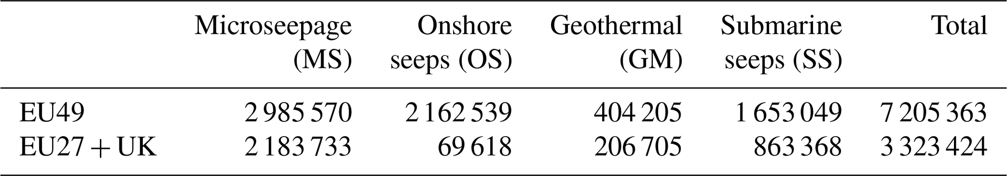
Table A5 compares the new results with previous European estimates (Etiope, 2009; Petrescu et al., 2021).

Table A5 European geo-CH₄ emission estimates (Tg yr⁻¹).

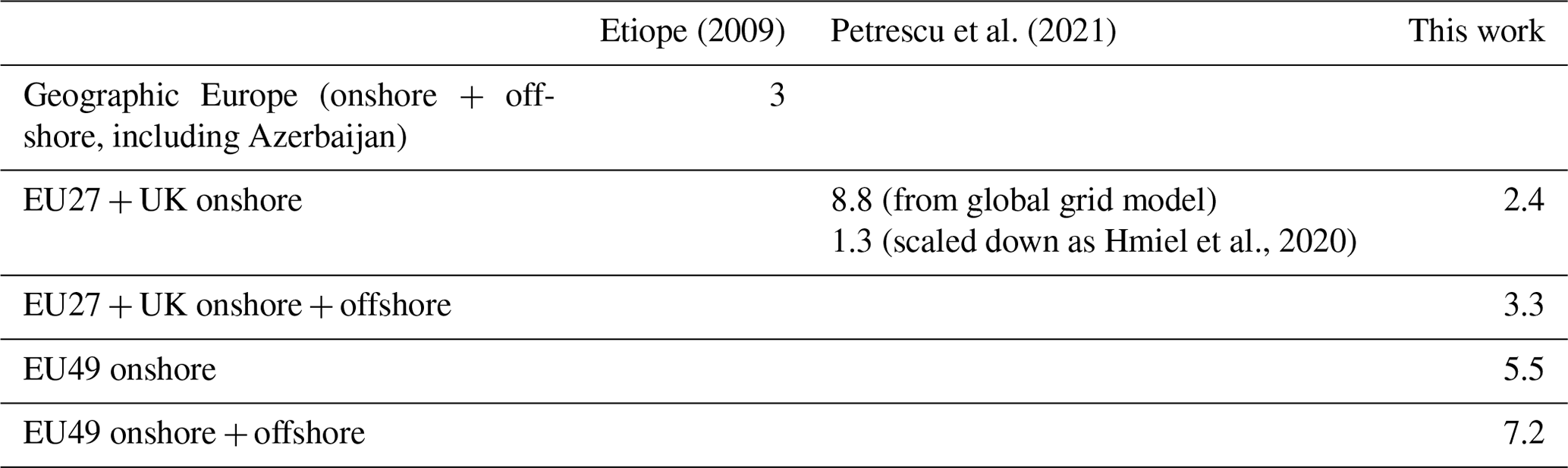
The overall uncertainties of the spatial distribution of the geo-CH₄ sources and CH₄ emissions depend on individual uncertainties of the four categories of seepage, which are discussed in Etiope et al. (2019). Compared to the global grid model, the uncertainty of the microseepage at European scale by refining the activity (microseepage area) has been reduced.

The new EU27 + UK geo-CH₄ emission estimate is lower than the one derived by Petrescu et al. (2021) using the global gridding but higher than the scaled-down value (Eq. A1). The EU49 (onshore + offshore) emission is higher than, but of the same order of magnitude of, the preliminary, rough estimate of geographic Europe, which included Azerbaijan, by Etiope (2009). Onshore geo-CH₄ emissions occur mostly in Azerbaijan, Italy and Romania, which are actually the EU49 countries with major onshore oil–gas reserves and production (BP, 2020) and thus with greater natural seepage potential. Offshore emissions are dominated by the large estimates published for the UK shelf (Judd et al., 1997, revised by Tizzard, 2008). These estimates need to be verified and improved. Beyond the emission values, our gridding provides, however, the first detailed map of natural geological methane emission in Europe, which can be used for continental-scale methane budget modeling.

A2.3 Top-down natural CH₄ emission estimates

Global Carbon Project – Global Methane Budget (Saunois et al., 2020)

For this study, none of the global inversions were updated.

GMB uses an ensemble of 13 monthly gridded estimates of wetland emissions based on different land surface models as calculated for Saunois et al. (2020). Each model conducted a 30-year spin-up and then simulated net methane emissions from wetland ecosystems over 2000–2017. The models were forced by CRU JRA (University of East Anglia Climatic Research Unit (CRU) Japanese Reanalysis (JRA)) reconstructed climate fields (Harris, 2019) and by the remote-sensing-based wetland dynamical area dataset WAD2M (Wetland Area Dynamics for Methane Modeling). This dataset provides monthly global areas over 2000–2017 based on a combination of microwave remote sensing data from Schroeder et al. (2015) and various regional inventory datasets. More information is available in Saunois et al. (2020), and more details will be presented in a future publication led by Poulter et al. (2017) and colleagues.

Uncertainty. As described by Saunois et al. (2020) uncertainties are reported as minimum and maximum values of the available studies, in brackets. They do not take into account the uncertainty of the individual estimates but rather express the uncertainty as the range of available mean estimates, i.e., the standard error across measurements/methodologies considered.

A3 Anthropogenic and natural N₂O emissions

A3.1 Bottom-up N₂O emission estimates

UNFCCC NGHGI (2019), EDGARv6.0 and CAPRI

Descriptions are found in Appendix A1.

ECOSSE

ECOSSE is a biogeochemical model that is based on the carbon model ROTH-C (Jenkinson and Rayner, 1977; Jenkinson et al., 1987; Coleman and Jenkinson, 1996) and the nitrogen model SUNDIAL (Bradbury et al., 1993; Smith et al., 1996). All processes of the carbon and nitrogen dynamics are considered (Smith et al., 2010a, b). Additionally, in ECOSSE processes of minor relevance for mineral arable soils are implemented as well (e.g., methane emissions) to have a better representation of processes that are relevant for other soils (e.g., organic soils). ECOSSE can run in different modes and for different time steps. The two main modes are site-specific and limited data. In the later version, basis assumptions/estimates for parameters can be provided by the model. This increases the uncertainty but makes ECOSSE a universal tool that can be applied for large-scale simulations even if the data availability is limited. To increase the accuracy in the site-specific version of the model, detailed information about soil properties, plant input, nutrient application and management can be added as available.

During the decomposition process, material is exchanged between the soil organic matter (SOM) pools according to first-order rate equations; characterized by a specific rate constant for each pool; and modified according to rate modifiers dependent on the temperature, moisture, crop cover and pH of the soil. The N content of the soil follows the decomposition of the SOM, with a stable C:N ratio defined for each pool at a given pH and with N being either mineralized or immobilized to maintain that ratio. Nitrogen released from decomposing SOM as ammonium (NH${}_{\mathrm{4}}^{+}$) or added to the soil may be nitrified to nitrate (NO${}_{\mathrm{3}}^{-}$).

For spatial simulations the model is implemented in a spatial model platform. This allows us to aggregate the input parameter for the needed resolution. ECOSSE is a one-dimensional model, and the model platform provides the input data in a spatial distribution and aggregates the model outputs for further analysis. While climate data are interpolated, soil data are represented by the dominant soil type or by the proportional representation of the different soil types in the spatial simulation unit (this is a grid cell in VERIFY).

Uncertainties in ECOSSE arise from three primary sources: parameters, forcing data (including spatial and temporal resolution), and model structure.

DayCent

DayCent was designed to simulate soil C dynamics, nutrient flows (N, P, S) and trace gas fluxes (CO₂, CH₄, N₂O, NO_x, N₂) between soil, plants and the atmosphere at a daily time step. Submodels include soil water content and temperature by layer, plant production and allocation of net primary production (NPP), decomposition of litter and soil organic matter, mineralization of nutrients, N gas emissions from nitrification and denitrification, and CH₄ oxidation in non-saturated soils.

The DayCent modeling application at the EU level is a consolidated model framework running on LUCAS point (Orgiazzi et al., 2018), which was extensively explained in previous works (Lugato et al., 2017, 2018; Quemada et al., 2020), where a detailed description of numerical and geographical datasets and uncertainty estimations is reported.

Information directly derived from LUCAS (2009–2015) included the soil organic carbon content (SOC), particle size distribution and pH. Hydraulic properties and bulk density were also calculated with an empirically derived pedotransfer function. Management information was derived from official statistics (EUROSTAT, 2019) and included crop shares at the NUTS2 level. The amount of mineral N was partitioned according to the regional crop rotations and agronomic crop requirements. Organic fertilization and irrigated areas were derived from the Gridded Livestock of the World FAO dataset and the FAO-AQUASTAT (2020) product.

Meteorological data were downloaded from the E-OBS gridded dataset (http://www.ecad.eu, last access: June 2019) at 0.1^∘ resolution. For the climatic projection, the gridded data from CORDEX database (https://esgf-node.ipsl.upmc.fr/search/cordex-ipsl/, last access: June 2019; CORDEX, 2020) were used. The average annual (2006–2010) atmospheric N deposition from the EMEP model (v4.5) were also implemented into the simulations. For current study, the results were updated and use the 2015–2019 mean.

Uncertainty. The starting year of the simulation was set to 2009 and projected in the future. The uncertainty analysis, based on the Monte Carlo approach, was done running the model 52 times in each point and, contemporary, randomly sampling model inputs from probability density functions for SOC pool partition, irrigation, and both mineral and organic fertilization rates. The model outputs (including uncertainties) at point level were upscaled regionally at 1 km resolution by a machine learning approach based on random forest regression.

N₂O emissions from inland waters

The N₂O estimate represents a climatology of average annual N₂O emissions from rivers, lakes, reservoirs and estuaries at the spatial resolution of 0.1^∘. Based on a spatially explicit representation of water bodies and point and non-point sources of N and P, this model quantifies the global-scale spatial patterns in inland water N₂O emissions in a consistent manner at 0.5^∘ resolution, which were then downscaled to 0.1^∘ using the spatial distribution of European inland water bodies. The procedure to calculate the cascading loads of N and P delivered to each water body along the river–reservoir–estuary continuum and to topologically connect 1.4 million lakes (extracted from the HydroLAKES database) is described in Maavara et al.(2019) and Lauerwald et al. (2019). The methodology to quantify N₂O emissions is based on the application of a MSM to estimate inland water C–N–P cycling as well as N₂O production and emission generated by nitrification and denitrification. Using a Monte Carlo analysis, the MSM allows us to generate relationships relating N processes and N₂O emissions to N and P loads and water residence time from the mechanistic model outputs, which are subsequently applied for the spatially resolved upscaling. For the estimation of N₂O emission, we ran two distinct model configurations relying on EFs scaling to denitrification and nitrification rates: one assuming that N₂O production equals N₂O emissions and the other taking into account the kinetic limitation on N₂O gas transfer and progressive N₂O reduction to N₂ during denitrification in water bodies with increasing residence time (Maavara et al., 2019). The model outputs from the two scenarios are used to constrain uncertainties in N₂O emission estimates.

For this study, the upscaled RECCAP2 estimates were used. This approach synthesizes existing inland water emission estimates for N₂O (Yao et al., 2020; Marzadri et al., 2021; Maavara et al., 2019; Lauerwald et al., 2019; Del Sontro et al., 2018; Deemer et al., 2016), homogenized and rescaled to a consistent set of inland water surface area (Messager et al., 2016; Allen and Pavelsky, 2018) and corrected for the effects of seasonal ice cover (Yang et al., 2020). It produced average annual N₂O emissions fluxes for Europe.

GAINS

Specific sectors and abatement technologies in GAINS vary by the specific emitted compound, with source sector definition and emission factors largely following the IPCC methodology at the Tier 1 or Tier 2 level. GAINS includes in general all anthropogenic emissions to air but does not cover emissions from forest fires, savannah burning and land use/land use change. Emissions are estimated for 174 countries/regions, with the possibility to aggregate to a global emission estimate and spanning a time frame from 1990 to 2050 in 5-year intervals. Activity drivers for macroeconomic development, energy supply and demand, and agricultural activities are entered externally; GAINS extends with knowledge required to estimate “default” emissions (emissions occurring due to an economic activity without emission abatement) and emissions and costs of situations under emission control (Amann et al., 2011).

Emissions of nitrous oxide derive from energy, industry, agriculture and waste. Land use change emissions are not included. In the energy sector, certain technologies implemented to improve air quality affect N₂O emission factors (like catalytic converters in vehicles), sometimes also negatively. That is also the case for non-selective catalytic reduction devices for NO_x abatement in power plants or for fluidized bed combustion. Relevant industrial processes cover nitric acid and adipic acid, with other processes (glyoxal, if relevant, or caprolactam) included. Both processes allow for two different levels of abatement technologies, and both are relatively easily accessible and low cost. The use of N₂O in gaseous form, often as an anesthetic for medical purposes, is associated with population numbers and scaled by availability of hospital beds. Marked emission reductions (at low costs) and a complete phaseout of emissions (high costs) are implemented as technologies. Agricultural emissions in part derive from manure handling, where different management strategies have repercussions on emissions. The larger fraction of emission is from application of nitrogen compounds in different forms to grassland, crops and rice, with rice using a different emission factor. Application of manure and of mineral fertilizer in GAINS can be reduced by advanced computer technology such as automatic steering and variable rate application or by agrochemistry (nitrification inhibitors). Costs of implementation are considered to depend on the size of a farm; hence, farm size is an important parameter. In the waste sector, composting and wastewater treatment are considered relevant sources. For wastewater treatment, GAINS also considers a specific emission reduction option when optimizing processes towards N₂O reduction (e.g., via favoring the anammox process). All details have been reported by Winiwarter et al. (2018) in their supplementary material.

Uncertainties. The same paper provides full information on the uncertainty of N₂O emissions in the GAINS model, which is a consequence of uncertainty provided in the activity data, in the emission factors and in the actual structure of the respective management strategies that also include the share of abatement technology already implemented. Further parameters also described (on uncertainty of future projections and on costs) are not relevant here.

FAOSTAT

The Statistics Division of the Food and Agriculture Organization of the United Nations provides N₂O emissions from agriculture (https://www.fao.org/faostat/en/#data/GT, last access: April 2022) and its sub-domains, as well as N₂O emissions from land use linked to biomass burning. The FAOSTAT emissions database is computed following Tier 1 of the 2006 IPCC Guidelines for National Greenhouse Gas Inventories (http://www.ipcc-nggip.iges.or.jp/public/2006gl/index.html, last access: January 2022). Country reports to FAO on crops, livestock and agriculture use of fertilizers are the source of activity data. Geospatial data are the source of AD for the estimates from cultivation of organic soils, biomass and peat fires. N₂O emissions are provided by country, regions and special groups, with global coverage, relative to the period of 1961–present (with annual updates, currently 2019) and with projections for 2030 and 2050 for agriculture only, expressed in both CO₂e and N₂O by underlying agricultural and land use emission sub-domain and by aggregate (agriculture total, agriculture total plus energy, agricultural soils). The main N₂O emissions are reported for the following agricultural activities: manure management, synthetic fertilizers, manure applied to the soils, manure left in pasture, crop residues, cultivation of organic soils and burning crop residues. LULUCF emissions consist of N₂O associated with burning biomass and peat fires, as well as from the drainage of organic soils. Comparison to the UNFCCC submissions is also provided.

Uncertainties were computed by Tubiello et al. (2013) but are not available in the FAOSTAT database.

A3.2 Top-down N₂O emission estimates

FLEXINVERT

The FLEXINVERT framework is based on Bayesian statistics and optimizes surface–atmosphere fluxes using the maximum probability solution (Rodgers, 2000). Atmospheric transport is modeled using the Lagrangian model FLEXPART (Stohl et al., 2005; Pisso et al., 2019) run in the backwards time mode to generate a so-called source–receptor matrix (SRM). The SRM describes the relationship between the change in mole fraction and the fluxes discretized in space and time (Seibert and Frank, 2004) and was calculated for 7 d prior to each observation. For use in the inversions, FLEXPART was driven using ECMWF ERA-Interim wind fields.

The state vector consisted of flux increments (i.e., offsets to the prior fluxes) discretized on an irregular grid based on the SRMs (Thompson and Stohl, 2014). This grid has a finer resolution (in this case the finest was 0.5^∘ × 0.5^∘) where the fluxes have a strong influence on the observations and a coarser resolution where the influence is only weak (the coarsest was 2^∘ × 2^∘). The flux increments were solved at 2-weekly temporal resolution. The state vector also included scalars for the background mole fractions. The optimal (posterior) fluxes were found using the conjugate gradient method (e.g., Paige and Saunders, 1975).

The background mole fractions, i.e., the contribution to the modeled mole fractions that is not accounted for in the 7 d SRMs, were estimated by coupling the termination points of backward trajectories (modeled using virtual particles) to initial fields of mole fractions from the optimized Eulerian model LMDZ (i.e., the CAMS-N₂O mole fraction product v18r1) following the method of Thompson and Stohl (2014).

Uncertainties. The posterior fluxes are subject to systematic errors primarily from (1) errors in the modeled atmospheric transport; (2) aggregation errors, i.e., errors arising from the way the flux variables are discretized in space and time; (3) errors in the background mole fractions; and (4) the incomplete information from the observations and hence the dependence on the prior fluxes. In addition, there is, to a smaller extent, some error due to calibration offsets between observing instruments, which is more pertinent for N₂O than for other GHGs. Random uncertainties are calculated from a Monte Carlo ensemble of inversions following Chevallier et al. (2007), and uncertainties in the observation space were inflated to take into account the model representation errors.

VERIFY Community Inversion Framework (CIF)

In the current study, new CIF results are presented (Berchet et al., 2021). For N₂O, inversions were run with CHIMERE and FLEXPART (NILU). The results using the two models were very comparable at the level of the EU27 plus Norway, Switzerland and the UK, with annual mean emissions for 2005–2018.

CHIMERE (see https://www.lmd.polytechnique.fr/chimere/, last access: May 2022) is a non-hydrostatic Eulerian chemistry–transport model. Its area-limited domains can be designed to cover the hemispheric to the urban scales, with horizontal resolutions from several degrees to 1 km. The time steps usually cover a few minutes, depending on the CFL and choices made by the user for minimizing computation costs. For the purpose of flux inversions, the tangent-linear and the adjoint codes have been developed and parallelized only for trace gases (see Fortems-Cheiney et al., 2021, their Sect. 3.2, for more details). The required input data are meteorological 3D and 2D fields (e.g., temperature, wind speed), boundary conditions for concentrations at the four sides and at the top of the domain, and emission fluxes. The comparison to surface measurements is done by extracting from the model the simulated concentrations in the grid cell matching the stations' locations for the time steps matching the measurement date and time. If the measurement covers a longer time (e.g., hourly means), the simulated concentrations for the matching time steps are averaged. For this deliverable, CHIMERE was run using meteorological data from the ECMWF's IFS operational forecast (every 3 h) retrieved at 0.25^∘ × 0.25^∘ and interpolated onto the model's grid (0.5^∘ × 0.5^∘). CHIMERE extends from the surface to 200 hPa with 17 sigma-pressure levels.

For the inversions provided by NILU, FLEXPARTv10.4 was run using ECMWF's operational IFS forecast with backward trajectory lengths of 7 d for N₂O. The footprints were saved at 0.5^∘ × 0.5^∘ for N₂O inversions. For N₂O anthropogenic emissions were taken from EDGARv6.0. An estimate for the natural N₂O flux was provided by the O-CN land surface model – a monthly climatology of the pre-industrial (or baseline) fluxes (Zaehle et al., 2011) and an estimate for the ocean N₂O flux was provided by the coupled ocean–biogeochemistry model, PlankTOM-v10 – also a monthly climatology (Buitenhuis et al., 2018).

Uncertainties. In the CIF, the uncertainties are described by matrices, with variances on the diagonal and covariances on the off-diagonal. They are called the prior error (for the error statistics on the prior controlled variables) and the observation error (for the error statistics on the difference between the observed and modeled mixing ratios). Observation errors were assumed to be independent from each other in all inversions; i.e., the observation error covariance matrix is diagonal. For CHIMERE, measurement errors were provided from observation files. Transport, representation and aggregation errors were deduced from the CH₄-based errors. For FLEXPART (NILU), the observation errors were calculated in the same way as for CH₄, but a minimum error of 0.3 ppb was used.

A3.3 Global N₂O Budget – GCP (Tian et al., 2020)

CAMS-N₂O

Within the GCP 2019 results, N₂O fluxes are estimated using the atmospheric inversion framework, CAMS-N₂O. Atmospheric inversions use observations of atmospheric mixing ratios, in this case, of N₂O, and provide the fluxes that best explain the observations while at the same time being guided by a prior estimate of the fluxes. In other words, the fluxes are optimized to fit the observations within the limits of the prior and observation uncertainties. To produce the optimized (a posteriori) fluxes, a number of steps are involved: first, the observations are pre-processed; second, a prior flux estimate is prepared; third, mixing ratios are simulated using the prior fluxes and are used to estimate the model representation error; and fourth, the inversion is performed. In total, 140 ground-based sites, ship and aircraft transects are included in the inversion. The term “site” refers to locations where there is a long-term record of observations and includes ground-based measurements, both from discrete samples (or “flasks”) and quasi-continuous sampling by in situ instruments, as well as aircraft measurements. A prior estimate of the total N₂O flux with monthly resolution and inter-annually varying fluxes is prepared from a number of models and inventories. For the soil fluxes (including anthropogenic and natural) an estimate from the land surface model OCN-v1.2 is used, which is driven by observation-based climate data, N-fertilizer statistics and modeled N deposition (Zaehle et al., 2011). For the ocean fluxes, an estimate from the ocean biogeochemistry model PlankTOM-v10.2 is used, which is a prognostic model (Buitenhuis et al., 2018). Atmospheric transport is modeled using an offline version of the Laboratoire de Météorologie Dynamique model, LMDZ5, which computes the evolution of atmospheric compounds using archived fields of winds, convection mass fluxes and planetary boundary layer (PBL) exchange coefficients that have been calculated using the online version nudged to ECMWF ERA-Interim winds.

CAMS-N₂O uses the Bayesian inversion method to find the optimal fluxes of N₂O, given prior information about the fluxes and their uncertainty, and observations of atmospheric N₂O mole fractions. The method is the same as that used in Thompson and Stohl (2014). For this study, inversions were not updated.

Uncertainty. Uncertainties in CAMS-N₂O simulations pertain to observation space and to state space. Uncertainty in the observation space is calculated as the quadratic sum of the measurement and transport uncertainties. The measurement uncertainty is assumed to be 0.3 ppb (approximately 0.1 %) based on the recommendations of data providers. The transport uncertainty includes estimates of uncertainties in advective transport (based on the method of Rödenbeck et al., 2003) and from a lack of subgrid-scale variability (based on the method of Bergamaschi et al., 2010). For the error in each land grid cell, the maximum magnitude of the flux in the cell of interest and its eight neighbors is used, while for ocean grid cells the magnitude of the cell of interest only is used. Posterior flux uncertainties are calculated from a Monte Carlo ensemble of inversions, based on the method of Chevallier et al. (2005).

TOMCAT-INVICAT

TOMCAT-INVICAT (Wilson et al., 2014) is a variational inverse transport model, which is based on the global chemical transport model TOMCAT and its adjoint. It uses a 4D variational (4DVAR) optimization framework based on Bayesian theory which seeks to minimize model–observation differences by altering surface fluxes while allowing for prior knowledge of these fluxes to be retained. TOMCAT (Monks et al., 2017) is an offline chemical transport model in which meteorological data are taken from ECMWF ERA-Interim reanalyses (Dee et al., 2011). The model grid resolution and therefore the optimized surface flux estimates have a horizontal resolution of 5.6×5.6^∘. The model has 60 vertical levels running from the surface to 0.1 hPa. For each individual year's fluxes, which are optimized on a monthly basis, 30 minimization iterations are carried out. For this study, inversions were not updated.

Uncertainty. Uncertainties in TOMCAT-INVICAT N₂O inversions are described as follows and further in Thompson et al. (2019). Uncertainty in the observations is calculated as the quadratic sum of the measurement and transport uncertainties. The measurement uncertainty for each observation is assumed to be 0.4 ppb, while the transport error of each observation is assumed to be the mean difference between the observation grid cell and its eight neighbors. Prior flux errors are assumed to be 100 % or the same as those of the prior estimates and are uncorrelated in space and time. Posterior flux uncertainties are not currently able to be calculated.

MIROC4-ACTM

The MIROC4-ACTM time-dependent inversion for the 84-region (TDI84) framework is based on Bayesian statistics and optimizes surface–atmosphere fluxes using the maximum probability solution (Rodgers, 2000). Atmospheric transport is modeled using the atmospheric chemistry–transport model (MIROC4-ACTM) based on JAMSTEC's Model for Interdisciplinary Research on Climate, version 4 (Watanabe et al., 2008; Patra et al., 2018, 2022). The source–receptor matrix (SRM) is calculated by simulating unitary emissions from 84 basis regions, for which the fluxes are optimized. The SRM describes the relationship between the change in mole fraction at the measurement locations for the unitary basis region fluxes (similar to Rayner et al., 1999). The MIROC4-ACTM meteorology was nudged to the JMA 55-year reanalysis (JRA55) horizontal wind fields and temperature. The simulated mole fractions for the total a priori fluxes are subtracted from the observed concentrations before running the inversion calculation (as in Patra et al., 2016, for CH₄ inversion).

In this study, the simulations have been updated to 2019 (Patra et al., 2022).

Uncertainties. The posterior fluxes are subject to systematic errors primarily from (1) errors in the modeled atmospheric transport; (2) aggregation errors, i.e., errors arising from the way the flux variables are discretized in space (84 regions) and time (monthly means); (3) errors in the background mole fractions (assumed to be a minor factor); and (4) the incomplete information from the sparse observational network and hence the dependence on the prior fluxes. In addition, there is, to a much smaller extent, some error due to calibration offsets between observing instruments, which is more pertinent for N₂O than for other GHGs. We have validated model transport in the troposphere using SF6 for the inter-hemispheric exchange time and using SF6 and CO₂ for the age of air in the stratosphere. The simulated N₂O concentrations are also compared with aircraft measurements in the upper troposphere and lower stratosphere for evaluating the stratosphere–troposphere exchange rates. Comparisons with ACE-FTS vertical profiles in the stratosphere and mesosphere indicate good parameterization of N₂O loss by photolysis and chemical reactions, and thus the lifetime, which affect the global total N₂O budgets.

Random uncertainties are calculated by the inverse model depending on the prior flux uncertainties and the observational data density and data uncertainty. Only 37 sites are used in the inversion, and thus the reduction in the prior flux uncertainties has been minimal. The net fluxes from the inversion from individual basis regions are less reliable compared to the anomalies in the estimated fluxes over a period of time.

Appendix B

B1 Overview figures

Figure B1 EU27 + UK total CH₄ emissions (a) and N₂O emissions (b) time series per sector as reported by UNFCCC NGHGI (2021).

Figure B2 EU27 + UK natural CH₄ emissions from Fig. 4b, as follows: two estimates for inland waters (lake, river and reservoir process-based models, blue, and upscaled emissions, cyan), peatlands and mineral soils (from JSBACH–HIMMELI, light green and dark green), geological emissions (orange), and biomass burning (from GFEDv4.1, brown).

B2 Source-specific methodology: AD, EF and uncertainties

Table B1 Source-specific activity data (AD), emission factors (EF) and uncertainty methodology for the current VERIFY and non-VERIFY 2021 data product collection.

Table B2 Biogeochemical models that computed wetland emissions used in this study. Runs were performed for the whole period of 2000–2017. Models run with prognostic (using their own calculation of wetland areas) and/or diagnostic (using WAD2M) wetland surface areas (see Sect. 3.2.1). From Saunois et al. (2020).

Table B3 Top-down studies used in our new analysis, with their contribution to the decadal and yearly estimates noted. For decadal means, top-down studies have to provide at least 8 years of data over the decade to contribute to the estimate, from Saunois et al. (2020).

Table B4 List of prior datasets for natural CH₄ and N₂O emissions used by all inverse models.