The consolidated European synthesis of CO₂ emissions and removals for the European Union and United Kingdom: 1990–2020

Quantification of land surface–atmosphere fluxes of carbon dioxide (CO₂) and their trends and uncertainties is essential for monitoring progress of the EU27+UK bloc as it strives to meet ambitious targets determined by both international agreements and internal regulation. This study provides a consolidated synthesis of fossil sources (CO₂ fossil) and natural (including formally managed ecosystems) sources and sinks over land (CO₂ land) using bottom-up (BU) and top-down (TD) approaches for the European Union and United Kingdom (EU27+UK), updating earlier syntheses (Petrescu et al., 2020, 2021). Given the wide scope of the work and the variety of approaches involved, this study aims to answer essential questions identified in the previous syntheses and understand the differences between datasets, particularly for poorly characterized fluxes from managed and unmanaged ecosystems. The work integrates updated emission inventory data, process-based model results, data-driven categorical model results, and inverse modeling estimates, extending the previous period 1990–2018 to the year 2020 to the extent possible. BU and TD products are compared with the European national greenhouse gas inventory (NGHGI) reported by parties including the year 2019 under the United Nations Framework Convention on Climate Change (UNFCCC). The uncertainties of the EU27+UK NGHGI were evaluated using the standard deviation reported by the EU member states following the guidelines of the Intergovernmental Panel on Climate Change (IPCC) and harmonized by gap-filling procedures. Variation in estimates produced with other methods, such as atmospheric inversion models (TD) or spatially disaggregated inventory datasets (BU), originate from within-model uncertainty related to parameterization as well as structural differences between models. By comparing the NGHGI with other approaches, key sources of differences between estimates arise primarily in activities. System boundaries and emission categories create differences in CO₂ fossil datasets, while different land use definitions for reporting emissions from land use, land use change, and forestry (LULUCF) activities result in differences for CO₂ land. The latter has important consequences for atmospheric inversions, leading to inversions reporting stronger sinks in vegetation and soils than are reported by the NGHGI.

For CO₂ fossil emissions, after harmonizing estimates based on common activities and selecting the most recent year available for all datasets, the UNFCCC NGHGI for the EU27+UK accounts for 926 ± 13 Tg C yr⁻¹, while eight other BU sources report a mean value of 948 [937,961] Tg C yr⁻¹ (25th, 75th percentiles). The sole top-down inversion of fossil emissions currently available accounts for 875 Tg C in this same year, a value outside the uncertainty of both the NGHGI and bottom-up ensemble estimates and for which uncertainty estimates are not currently available. For the net CO₂ land fluxes, during the most recent 5-year period including the NGHGI estimates, the NGHGI accounted for −91 ± 32 Tg C yr⁻¹, while six other BU approaches reported a mean sink of −62 [$-\mathrm{117},-\mathrm{49}$] Tg C yr⁻¹, and a 15-member ensemble of dynamic global vegetation models (DGVMs) reported −69 [$-\mathrm{152},-\mathrm{5}$] Tg C yr⁻¹. The 5-year mean of three TD regional ensembles combined with one non-ensemble inversion of −73 Tg C yr⁻¹ has a slightly smaller spread (0th–100th percentiles of [$-\mathrm{135},+\mathrm{45}$] Tg C yr⁻¹), and it was calculated after removing net land–atmosphere CO₂ fluxes caused by lateral transport of carbon (crop trade, wood trade, river transport, and net uptake from inland water bodies), resulting in increased agreement with the NGHGI and bottom-up approaches. Results at the category level (Forest Land, Cropland, Grassland) generally show good agreement between the NGHGI and category-specific models, but results for DGVMs are mixed. Overall, for both CO₂ fossil and net CO₂ land fluxes, we find that current independent approaches are consistent with the NGHGI at the scale of the EU27+UK. We conclude that CO₂ emissions from fossil sources have decreased over the past 30 years in the EU27+UK, while land fluxes are relatively stable: positive or negative trends larger (smaller) than 0.07 (−0.61) Tg C yr⁻² can be ruled out for the NGHGI. In addition, a gap on the order of 1000 Tg C yr⁻¹ between CO₂ fossil emissions and net CO₂ uptake by the land exists regardless of the type of approach (NGHGI, TD, BU), falling well outside all available estimates of uncertainties. However, uncertainties in top-down approaches to estimate CO₂ fossil emissions remain uncharacterized and are likely substantial, in addition to known uncertainties in top-down estimates of the land fluxes. The data used to plot the figures are available at https://doi.org/10.5281/zenodo.8148461 (McGrath et al., 2023).

1 Introduction

Atmospheric mole fractions of greenhouse gasses (GHGs) reflect a balance between emissions from both human activities and natural sources and removals by the terrestrial biosphere, oceans, and atmospheric oxidation. Increasing levels of GHGs in the atmosphere due to human activities have been the major driver of climate change since the pre-industrial period (IPCC, 2021). In 2020, GHG mole fractions reached record highs, with globally averaged mole fractions of 413.2 ppm (parts per million) for carbon dioxide (CO₂), representing 149 % of the pre-industrial level (WMO, 2021). The rise in CO₂ mole fractions in recent decades is caused primarily by CO₂ emissions from fossil sources. Globally, fossil emissions in 2020 (excluding the cement carbonation sink) totaled 9500 ± 500 Tg C yr⁻¹, with expectations to rise in 2021 as the world recovered from the first year of the Covid-19 pandemic (Friedlingstein et al., 2022). In contrast, global net CO₂ emissions from land use and land use change (LULUC, primarily deforestation; see glossary in Table A1 for more details), estimated from bookkeeping models and dynamic global vegetation models (DGVMs), were estimated to have a small decreasing trend over the past 2 decades, albeit with low confidence, and a value in the year 2020 of 900 ± 700 Tg C yr⁻¹ (Friedlingstein et al., 2022). This decrease, however, is almost an order of magnitude less than the growth in fossil emissions over the same period; therefore, the total fossil and net LULUC flux has still increased.

As all countries in the EU27+UK are Annex I Parties¹ to the United Nations Framework Convention on Climate Change (UNFCCC), they prepare and report national GHG inventories (NGHGIs) on an annual basis. These inventories contain annual time series of each country's GHG emissions from the 1990 base year² until 2 years before the year of reporting and were originally set to track progress towards their reduction targets under the Kyoto Protocol (UNFCCC, 1997). Annex I NGHGIs are reported according to Decision 24/CP.19 of the UNFCCC Conference of the Parties (COP), which states that the national inventories shall be compiled using the methodologies provided in the 2006 IPCC Guidelines for National Greenhouse Gas Inventories (IPCC, 2006). The 2006 Intergovernmental Panel on Climate Change (IPCC) guidelines provide methodological guidance for estimating emissions for well-defined sectors using national activity and available emission factors. Decision trees indicate the appropriate level of methodological sophistication (“tiered methods”) based on the absolute contribution of the sector to the national GHG balance and the country's national circumstances (availability and resolution of national activity data and emission factors). Generally, Tier 1 methods are based on global or regional default emission factors that can be used with aggregated activity data, while Tier 2 methods rely on country-specific factors and/or activity data at a higher category resolution. Tier 3 methods are based on more detailed process-level modeling or in some cases facility-level emission observations. Annex I Parties are furthermore required to estimate and report uncertainties in emissions (95 % confidence interval), following the 2006 IPCC guidelines using, as a minimum requirement, the Gaussian error propagation method (approach 1). Annex I Parties are furthermore encouraged to use Monte Carlo methods (approach 2) or a hybrid approach. Additional information on the NGHGIs can be found in Appendix A2.

In addition to the NGHGIs, other research groups and international institutions produce independent estimates of national GHG emissions with two approaches: atmospheric inversions (top-down, TD) and GHG inventories based on the same principle as NGHGIs but using slightly different methods (tiers), activity data, and/or emission factors (bottom-up, BU). The current work has a strong focus on the EU27 and therefore sits within the context of recent legislation passed by the European Parliament concerning commitments for the land use, land use change, and forestry (LULUCF) sector to achieve the objectives of the Paris Agreement and the reduction target for the union (EU, 2018a, and the proposed amendments, EU, 2021a). This legislation requires that, “Member States shall ensure that their accounts and other data provided under this Regulation are accurate, complete, consistent, comparable, and transparent”. The TD and BU methods discussed below include the most up-to-date publicly available spatially explicit information, which can help provide a quality check and increase public confidence in NGHGIs.

The work presented in this paper covers dozens of distinct datasets and models, in addition to the individual country submissions to the UNFCCC of the EU member states and the UK. As Annex I Parties, the NGHGIs of the EU member states and the UK are consistent with the general guidance laid out in IPCC (2006) yet still differ in specific approaches, models, and parameters, in addition to definitional differences in the underlying system boundaries and activity datasets. For the land-based sector, member states are only required to report terrestrial biospheric fluxes from managed lands instead of distinguishing between direct and indirect human-induced and natural effects on carbon fluxes for all ecosystems (Grassi et al., 2018a, 2022). This “managed land proxy” avoids having to quantify, for example, increased carbon uptake in remote Forest Land due to reactive nitrogen emissions from both natural soils and human-applied synthetic fertilizers. A comprehensive investigation of detailed differences between all datasets is beyond the scope of this paper, though systematic analyses have been previously made for specific sectors (e.g., AFOLU,³ Petrescu et al., 2020; previous synthesis to this work, Petrescu et al., 2021; FAOSTAT versus UNFCCC NGHGIs, Tubiello et al., 2021, and Grassi et al., 2022; UNFCCC versus bookkeeping models, Grassi et al., 2023; and UNFCCC versus inversions, Deng et al., 2021) and by the Global Carbon Project CO₂ syntheses (e.g., Friedlingstein et al., 2022).

Every year (time t) the Global Carbon Project (GCP) in its global carbon budget (GCB) quantifies large-scale CO₂ budgets up to the previous year (t−1), bringing in information from global to wide latitude bands, including various observation-based flux estimates from BU and TD approaches (Friedlingstein et al., 2022). The current paper, given the focus on a single region (Europe) with extensive data coverage, dives into more detail than the GCB, including category-specific models related to LULUCF (e.g., Forest Land, Grassland, Cropland) and making heavy use of the EU27+UK NGHGI in an effort to advance a trust-building process by mutual understanding developed though comparison of both approaches. Compared to Petrescu et al. (2021), the current work updates datasets, methods, and uncertainties.

BU observation-based approaches used in the GCB rely heavily on statistical data combined with Tier 1 and Tier 2 approaches. In the current work, focusing on a region that is well covered with data and models (EU27+UK), BU also refers to Tier 3 process-based models (see Sect. 2). At regional and country scales, systematic and regular comparison of these observation-based CO₂ flux estimates with reported fluxes under the UNFCCC is more difficult. Continuing our previous efforts within the European project VERIFY (VERIFY, 2022), the current study compares observation-based flux estimates of BU versus TD approaches and compares them with NGHGIs for the EU27+UK bloc and five subregions. VERIFY also provides, as a first attempt, similar comparisons for all European countries (VERIFY Synthesis Plots, 2022). The methodological and scientific challenges to compare these different estimates have been partly investigated before (Pongratz et al., 2021; Grassi et al., 2018a, for LULUCF; Andrew, 2020, for fossil sectors), but such comparisons were not done in a systematic and comprehensive way, including both fossil and land-based CO₂ fluxes, before Petrescu et al. (2021).

As the study by Petrescu et al. (2021) is the most comprehensive comparison of the NGHGIs and research datasets (including both TD and BU approaches) for the EU27+UK to date, the focus of the current paper is on improvement of estimates in the most recent version in comparison with the previous one, including changes in the uncertainty estimates and identification of the knowledge gaps and added value for policymaking. Official NGHGI emissions are compared with research datasets, including necessary harmonization of the latter on total emissions to ensure consistency. Differences and inconsistencies between emission estimates were analyzed, and recommendations were made towards future evaluation of NGHGI data. It is important to remember that, while NGHGIs include uncertainty estimates, the “uncertainty analysis should be seen, first and foremost, as a means to help prioritize national efforts to reduce the uncertainty of inventories in the future and guide decisions on methodological choice” (Vol. 1, Chap. 3, IPCC, 2006) and were therefore not developed to enable comparisons between countries or other datasets. In addition, individual spatially disaggregated research emission datasets often lack quantification of uncertainty. Here, we focus on the mean value and various percentiles (0th, 25th, 75th, 100th) of different research products of the same type to get a first estimate of uncertainty (see Sect. 2). Not all models/inventories provided an update for v2021; therefore, for the non-updated datasets, the previously published time series are shown.

The dataset assembled in this paper (McGrath et al., 2023) provides annual values of carbon dioxide emissions and sinks in fossil and LULUCF sectors for the EU27+UK across a range of data products based on different methodologies. This enables, for example, researchers to produce datasets based on new methods and also provides a source of evaluation in the form of a best-estimate range of values. Decision-makers may also find the results useful for targeting mitigation efforts in the EU27+UK by providing a more complete subsectorial breakdown. While NGHGIs already provide detailed data-based disaggregation based on activities, the dataset here adds additional constraints from independent data and models used outside of the inventory community. In addition, this paper outlines a methodology by which users of country-level CO₂ emission data can compare datasets against NGHGIs and identify where agreement occurs for the right (and wrong) reasons.

Section 3.1 highlights the extreme difference between current fossil emissions and uptake by the land surface. Section 3.2 looks at an ensemble of bottom-up estimates of fossil CO₂ emissions, in addition to a preliminary inversion using atmospheric NO₂ observations as a constraint. Section 3.3.2 and 3.3.3 show that better agreement between the NGHGI and other models occurs when the models are driven strongly be category-specific data in forestry, grasslands, and croplands, as opposed to more generalized models created to couple to atmospheric models in global climate projections. Section 3.3.4 highlights the challenges currently facing the comparison of atmospheric inversion models with NGHGIs while simultaneously showing improvement by accounting for net emissions for lateral transfer of carbon between countries. Section 3.4 provides more discussion around uncertainties in both top-down and bottom-up estimates.

A list of acronyms and terminology is provided in Table A1 for easy reference.

2 CO₂ data sources and estimation approaches

The CO₂ emissions and removals in the EU27+UK estimated by inversions and anthropogenic emission inventories resolved at the source category level were analyzed. At the time of this work, data of CO₂ fossil emissions and CO₂ land⁴ emissions and removals (Tables 1 and 2) covered the period from 1990 to 2020, with some of the data only available for shorter time periods. Since then, some datasets have been updated to include 2021, but not all, and we made the decision to stay with the original time window for simplicity. The estimates are available both from peer-reviewed literature and from new research results from the VERIFY project. BU results are compared to NGHGIs reported in 2021 (which contain the time series for 1990–2019). Data sources are summarized in Tables 1 and 2 with the detailed description of all products provided in Appendix A2–A4. In Appendix A2, the harmonized methodology for calculation of uncertainties submitted by member states to the UNFCCC in their national inventory reports (NIRs) is explained. This includes the same 95 % confidence interval as is typically reported but involved an extensive gap-filling to cover more categories and more years than available in Petrescu et al. (2021), which limited uncertainty estimation to a single year.

BU anthropogenic CO₂ fossil estimates include global inventory datasets such as the Emissions Database for Global Atmospheric Research (EDGAR v6.0.), Statistical Review of World Energy by BP, the Carbon Dioxide Information Analysis Center (CDIAC), the Global Carbon Project (GCP), the Energy Information Administration's (EIA) “International” dataset, and the International Energy Agency (IEA) (see Table 1). These datasets are all described in detail by Andrew (2020). CO₂ land emission estimates are derived from BU biogeochemical models (e.g., DGVMs, bookkeeping models; see Table 2). TD approaches include both high-spatial-resolution regional inversions (CarboScopeReg (CSR), EUROCOM (Monteil et al., 2020), inversions based on the CIF-CHIMERE system (Berchet et al., 2021), and LUMIA) and coarser-spatial-resolution global inversions (GCP 2021: Friedlingstein et al., 2022). Most of the inversions were carried out for CO₂ land emissions, with only a single inversion for CO₂ fossil emissions (CIF-CHIMERE). Note that CIF-CHIMERE provides estimates for both CO₂ land and CO₂ fossil from separate simulations. These estimates are described in Sect. 2.3.

The sign of the fluxes is defined from an atmospheric perspective: positive values represent a net source to the atmosphere and negative values a net removal from the atmosphere. As an overview of potential uncertainty sources, Table C1 presents the use of emission factor (EF) data, activity data (AD), and (whenever available) uncertainty methods used for all CO₂ land data sources in this study, in addition to more details on each model in Appendix A. The referenced data used for figure replicability purposes are available for download (McGrath et al., 2023). Upon request, the codes necessary to plot the figures in the same style and layout can be provided. The focus is on the EU27+UK emissions. In the VERIFY project, an additional web tool was developed which allows for the selection and display of all plots shown in this paper, not only for the EU member states and UK but also for a total of 79 countries and groups of countries in Europe (Table A2, Appendix A). The data are free of cost and can be accessed upon registration (VERIFY Synthesis Plots, 2022). An overview of the datasets, including contact information, is provided in Table C1.

For the sake of harmonization, we report the mean values of all ensembles. For small sample sizes (e.g., the regional inversions of CSR with four members), the literature does not give a clear indication on whether the mean or the median is preferred; a preference for one or the other depends on what one wishes to demonstrate. While the mean and median converge in the case of independent randomly distributed data, the median downplays data skewness. We display the mean for all ensembles. As the number of datasets in some ensembles is small (less than five), we display the minimum and maximum annual values for every year (i.e., the 0th/100th percentiles) to give an idea of the spread. For ensembles with more than 10 members (i.e., TRENDY), we show the mean and the 0th/100th percentiles along with the 25th/75th percentiles in the figures. This combination demonstrates “more likely” and “possible” behavior; as only one ensemble has both bars, displaying them does not overwhelm the reader much more than the standard graphs, and we find the added information to be worth the trade-off. In the text, we report the mean and 0th/100th percentiles for small ensembles and mean along with the 25th/75th for larger ensembles. We make every effort to limit the number of significant figures as a function of the error bars. In some cases (e.g., asymmetric error bars which overlap zero), we retain an extra significant figure to improve readability.

The current work extends Petrescu et al. (2021) by updating the included datasets (both increasing the number of years covered and in some cases updating the model versions), adding datasets, and highlighting changes in terms of mean annual emissions and trends. For clarity, the data from Petrescu et al. (2021) are labeled as v2019, while the latest results are labeled v2021.

2.1 CO₂ anthropogenic emissions from the NGHGI

The UNFCCC NGHGI (2021) estimates for the period 1990 to year t−2 (2019), collected for the EU27 and UK, are the basis for this dataset. For historical reasons, a few EU countries provide data for a different base year than 1990 (see footnote 2 above), yet it should be noted that regardless of the base year all countries of the EU27+UK bloc are obliged to report estimates for the period 1990 to year t−2. The Annex I Parties to the UNFCCC are required to report annual GHG inventories that include a NIR, with qualitative information on data and methods and a common reporting format (CRF) set of tables that provide quantitative information on GHG emissions by category. This annually updated dataset includes anthropogenic emissions and removals. For the land-based sector, the managed land proxy is used as a way to report only anthropogenic fluxes (Grassi et al., 2018a, 2022). This proxy allows member states to report all fluxes coming from land designed as “managed” without trying to disentangle their natural and anthropogenic origins. Spatially explicit maps of managed lands are not currently available, even for the relatively data-rich region of the European Union and United Kingdom. However, most of the European Union is classified by the member states as managed land; current estimates from available country-aggregated data indicate only 5 % of land in the EU is unmanaged, including some Forest Land, Grassland, and Wetlands. Figure B1 shows the annual NGHGI (2021) anthropogenic CO₂ time series disaggregated by sector in order to provide context.

2.2 CO₂ fossil emissions

CO₂ fossil emissions occur when fossil carbon compounds are broken down via combustion or other non-combustive industrial processes. Most of these fossil compounds are in the form of fossil fuels, such as coal, oil, and natural gas. Another source category of fossil CO₂ emissions is fossil carbonates, such as calcium carbonate and magnesium carbonate, which are used in industrial processes. Because CO₂ fossil emissions are largely connected with energy, which is a closely tracked commodity group of high economic importance, there is a wealth of underlying data that can be used for estimating emissions. However, differences in collection, treatment, interpretation, and inclusion of various factors – such as carbon contents and fractions of the fuel's carbon that is oxidized – lead to methodological differences (Appendix A3), resulting in differences in emissions between datasets (Andrew, 2020). The datasets are also not fully independent, as discussed in Sect. 2.4. Atmospheric inversions for emissions of fossil CO₂ are not as established as their bottom-up counterparts (Brophy et al., 2019). The main reason is that the types of atmospheric measurements suitable for fossil CO₂ atmospheric inversions have not yet been widely deployed (Ciais et al., 2015). One of the rare inversions is presented below.

In this analysis, the inventory-based bottom-up CO₂ fossil emission estimates are separated and presented per fuel type and reported for the last year when all data products are available (2017). This updates Andrew (2020) and Petrescu et al. (2021), which both report the year 2014. In order to provide a quasi-independent estimate of fossil emissions assimilating satellite observations of the atmosphere subject to current capabilities of atmospheric inversions, the CIF-CHIMERE model was used to produce a fossil fuel CO₂ emission estimate for the year 2017. CIF-CHIMERE is a coupling between the variational mode of the Community Inversion Framework (CIF) platform developed in the VERIFY project (Berchet et al., 2021), the CHIMERE chemical transport model (Menut et al., 2013), and the adjoint of this model (Fortems-Cheiney et al., 2021). To overcome the lack of CO₂ observation networks suitable for the monitoring of fossil CO₂ emissions at national scale, this inversion is based on the assimilation of satellite NO₂ data, which are representative of NO_x emissions, as NO_x is co-emitted with CO₂ during fossil fuel combustion. The uncertainties in the anthropogenic activities underlying the fossil fuel combustion are shared by both CO₂ and co-emitted species. Therefore, in principle, information from co-emitted species such as NO_x and CO can be used to decrease the uncertainties in fossil fuel CO₂ emissions. Recent top-down inversions of anthropogenic CO₂ emissions from Europe indicate that uncertainties using satellite measurements of NO₂ are much lower than for co-emitted CO when deriving fossil CO₂ emissions (Konovalov et al., 2016). Therefore, results shown below only incorporate NO₂ and not CO observations. The CHIMERE model includes a full chemistry scheme to enable linkage of observations of atmospheric NO₂ mole fractions to surface NO_x emissions. While the spatial and temporal coverage of the NO₂ observations is large, there are many factors that contribute to uncertainty in fossil fuel emission activity data, including the uncertainties in NO_x emission factors and thus the ratio of NO_x to CO₂ emissions. Therefore, the influence of using NO₂ observations in determining fossil CO₂ emissions is subject to uncertainties which have not been characterized appropriately yet in the framework of VERIFY. Here, this conversion relies heavily on the emission ratios per country, month, and large sector of activity from the TNO-GHGco-v3 inventory (Dellaert et al., 2021), which has been partly developed in VERIFY and which is based on the most recent UNECE-CLRTAP⁵ and UNFCCC official country reporting, respectively, for air pollutants and greenhouse gasses. The detailed descriptions of each of the data products are found in Appendix A3.

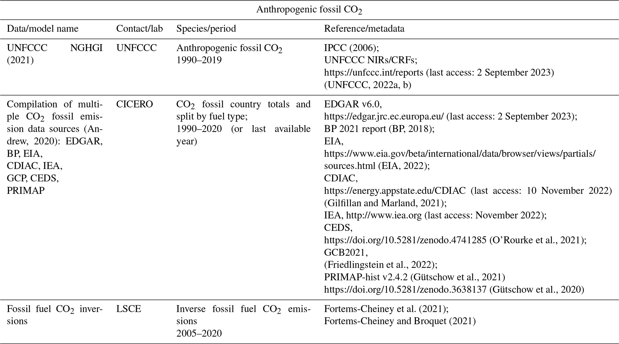
Table 1 Data sources for the anthropogenic CO₂ fossil emissions included in this study, all updated from Petrescu et al. (2021).

2.3 CO₂ land fluxes

Data products from BU and TD CO₂ land fluxes including CO₂ emissions and removals from land use, land use change, and forestry (LULUCF) activities are summarized in Table 2. All models and approaches produce an estimate of the net carbon flux from the land surface including uptake through photosynthesis and emission through respiration and/or disturbances. The details may vary significantly between approaches, however. Attempts are made where possible to harmonize input data and compare results which roughly correspond to similar categories included in the NGHGI. Further details are described throughout the rest of this article. As with CO₂ fossil fluxes, the primary distinctions are between the NGHGI, other bottom-up approaches, and top-down approaches. The situation becomes more complicated for CO₂ land fluxes due to the inclusion of approaches which only address a single land use category (e.g., Forest Land).

For the analysis at category level, the CO₂ net emissions from the LULUCF sector that are primarily considered in this synthesis are from three land use categories⁶ (Forest Land, Cropland, and Grassland), each split into a land category remaining in the same land category⁷ or a land category converted to another category. The NGHGI is the only result discussed here which makes use of this transition period, but the distinction is important so as to inform which NGHGI categories to use in the comparison. Wetlands, Settlements, Other land, and Harvested wood products (i.e., HWP) categories are included in the discussion on total LULUCF activities in Sect. 3.3.1 and 3.3.4. Not all the categories reported to the UNFCCC are present in FAOSTAT or other models. Some models are category specific (e.g., Forest Land), while other models include a larger subset of the six UNFCCC categories (e.g., DGVMs which simulate Forest Land, Grassland, and Cropland). The notations FL, CL and GL are used to indicate total emissions and removals from the respective Forest Land, Cropland, and Grassland land use categories (i.e., the remaining plus conversions to these categories). The notations “FL-FL”, “CL-CL”, and “GL-GL” are used to indicate emissions and removals from respective forest, cropland, and grassland areas which have remained in the same category from year to year or in the case of NGHGI lands that have not undergone conversion within the aforementioned transition period (e.g., t−20). Uncertainties for FL, CL, and GL are reported as percentages by the European Union, and we use them directly. An uncertainty greater than 100 % implies that either a sink or a source is possible.

The results from category-specific models reporting carbon fluxes for FL-FL (EFISCEN-Space and CBM), CL, and GL (EPIC-IIASA and ECOSSE) are presented separately from the models and datasets including multiple land use categories and simulating land use changes: FAOSTAT (version 2021), the DGVM ensemble TRENDY v10 (Friedlingstein et al., 2022; Le Quéré et al., 2009), the ORCHIDEE and CABLE-POP DGVMs forced by high-resolution meteorological data as part of the VERIFY project, and the two bookkeeping approaches of H&N (Houghton and Nassikas, 2017) and BLUE (bookkeeping of land use emissions; Hansis et al., 2015). BLUE includes two simulations with different land use forcing: one made for the VERIFY H2020 project (BLUE-vVERIFY) and one for GCB2021 (BLUE-vGCB) (Friedlingstein et al., 2022). For CL and GL, both the EPIC-IIASA and ECOSSE category-specific models reported updates, although ECOSSE only updated results for GL. Processes included in all the products are summarized in Appendix A2–A4 and Table C2.

The two updated inverse model ensembles presented are the GCB2021 for the period 2010–2020 (Friedlingstein et al., 2022) and EUROCOM for the period 2009–2018 (Monteil et al., 2020; Thompson et al., 2020). The GCB inversions are global and include CarbonTracker Europe (CTE: van der Laan-Luijkx et al., 2017), CAMS (Chevallier et al., 2005), Jena CarboScope (Rödenbeck, 2005), NISMON-CO₂ (Niwa et al., 2017), CMS-Flux (Liu et al., 2021), and UoE (Feng et al., 2016). The EUROCOM inversions are regional, with a domain limited to Europe and higher spatial resolution atmospheric transport models, with four inversions covering the entire period 2009–2018 as analyzed in Thompson et al. (2020). All inversions provide net ecosystem exchange (NEE) fluxes. These inversions make use of more than 30 atmospheric observing stations within Europe, including flask data and continuous observations, and work at typically higher spatial resolution than the global inversion models (Table 2). The prior anthropogenic emissions provided for all regional inversions reported here (i.e., EUROCOM, EUROCOM drought 2018, VERIFY CSR, VERIFY CIF-CHIMERE, and VERIFY LUMIA) are all based on EDGAR v4.3, BP statistics, and TNO datasets by generating spatial and temporal distributions through the COFFEE approach (Steinbach et al., 2011). Small differences exist between exact versions used by the different groups. The prior anthropogenic emissions for the GCB global inversions, GridFEDv2021, and v2022 are also based on EDGARv4.3.2 (Janssens-Maenhout et al., 2019). Differences in fossil fuel emissions for the regional inversions only exist for the years 2019 and 2020, and they only concern the temporal variation within the year not the annual totals per pixel (or country). Therefore, differences in the prior anthropogenic emissions are not expected to explain the large differences seen between the different regional biogenic inversions nor between the regional and global biogenic inversions, but efforts should be continued to harmonize them to the greatest extent possible in future intercomparisons.

Additional inversions for Europe from three regional-scale inversion systems are analyzed. Two of these systems are part of the EUROCOM ensemble, but new runs were carried out for the VERIFY project. The CarboScopeRegional (CSR) inversion system has performed additional runs for VERIFY for the years 2006–2020 with multiple ensemble members differing by biogenic prior fluxes and assimilated observations. The results are plotted separately to illustrate two points: (1) the CSR simulations for VERIFY are not identical to those submitted to EUROCOM (VERIFY runs from CSR included several sites that started shortly before the end of the EUROCOM inversion period), and (2) the CSR model was used in four distinct runs in VERIFY. Note that the ensemble members differ from previous years (the spatial correlation length is kept constant this year, while more prior fluxes are used). By presenting CSR separate from the EUROCOM results, one can get an idea of the uncertainty due to various model parameters in one inversion system with one single transport model. The LUMIA inversion system submitted four simulation results to the VERIFY project, based on the setup developed for the 2018 Drought Task Force project (labeled here as EUROCOM; Thompson et al., 2020), but with a refined definition of both prior and observation uncertainties. Also, for the years 2019–2020, the transport models (FLEXPART and TM5) were driven by ERA5 meteorological data, whereas for previous years ERA-Interim data were used. The four different variants include one reference simulation and three simulations which change spatial correlation lengths, the number of observation sites, and the magnitude of uncertainties in the boundary conditions. As one of the variants is only available for 2019–2020 (changing the uncertainties in the boundary conditions), this variant was dropped from the results and only the remaining three simulations are presented, covering the period 2006–2020.

An inversion of the NEE over 2005–2020 from the CIF-CHIMERE variational inversion system is also analyzed. The configuration of this inversion is close to that of the PYVAR-CHIMERE NEE inversions in the EUROCOM ensembles and follows the general principles of Broquet et al. (2013). However, it uses distinct inputs, which play a critical role in the inversion, such as a more recent ORCHIDEE simulation as prior estimate of the NEE and a more recent CAMS global inversion to impose the regional CO₂ boundary conditions.

Table 2 Data sources for the land CO₂ emissions included in this study. Details are found in Appendix A4. The time steps 1Y, 1M, 1W, and 3H refer to the availability of the data: “1 year”, “1 month”, “1 week”, and “3 h”, respectively. An overview of the datasets, including contact information, is provided in Table C1.

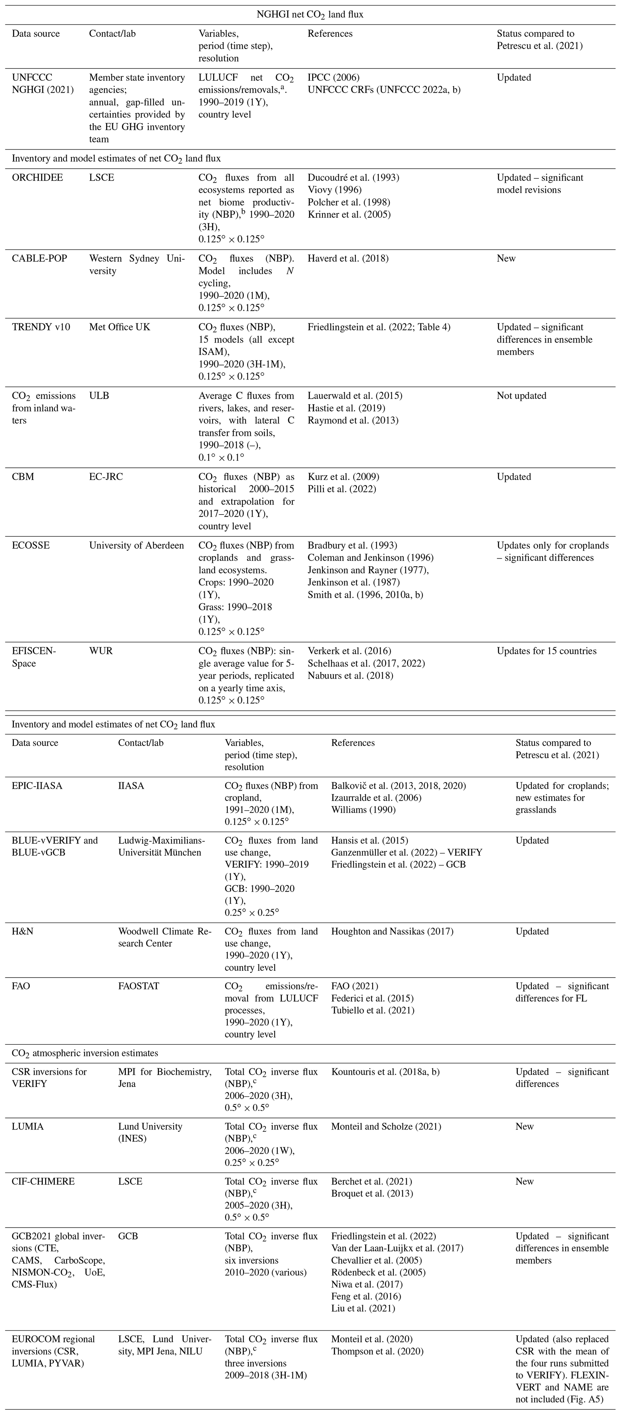
^a Member states use a mix of gain–loss and stock-change reporting methods (Table 6.12 in EU NIR, 2021). The net flux from a given country can thus be based on either stock changes or flux changes. ^b The definition of NBP various from model to model. Most models include harvest but not necessarily other disturbances. Please refer to Table C2 for more details. ^c The net carbon flux from regional inversions over land is the residual after fixing fossil CO₂ emissions and CO₂ fluxes from biomass burning. In other words, any flux not included in those two categories is reflected in the net flux from the inversions. Biomass burning is prescribed in two of the EUROCOM models (LUMIA and FLEXINVERT+; see Monteil et al., 2020, and Thompson et al., 2020) and ignored (i.e., assumed negligible in Europe) for the others.

All of the bottom-up models in this work require external forcing datasets. In the context of the VERIFY project (VERIFY, 2022), an effort was made to provide a single, harmonized version of several kinds of data (meteorological, land use/land cover, and nitrogen deposition) on a high-resolution grid over Europe. These datasets were then made available to all of the modeling groups to use in their simulations. Such a practice is common in model intercomparison projects. However, as the models in Table 2 are not all the same type, data harmonization presented more of a challenge in this work as not all models use the same inputs. All of the datasets described in Appendix A5 were used by at least one modeling group in this work.

2.4 Independence of estimates

As pointed out by Andrew (2020), bottom-up fossil CO₂ emission datasets are not entirely independent, since they largely rely on activity data reported by national agencies. However, there is some variation here, particularly in traded energy products where, for example, activity data may be sourced from either the exporter or the importer according to some determination of reporting reliability. However, beyond the underlying activity data, other choices do vary between datasets: emission factors, which specific products lead to emissions, and how the activity data are used to estimate the amount of energy product that is consumed, among others. Some examples of differences include the following: CDIAC avoids using reported energy consumption and relies on estimating apparent consumption from the major energy flows, CEDS initially used a very different estimate for emissions from international shipping, EDGAR and IEA use a Tier 1 approach with default emission factors, and PRIMAP-hist and GCP use officially reported emissions based on higher-tier methods and country-specific emission factors for selected countries. Further, the emission sources covered can vary widely between datasets, with the IEA usually limited to emissions from energy products, while EDGAR, for example, attempts to include all fossil CO₂ sources. With this lack of full independence between dataset sources and methods, the uncertainty ranges should be interpreted with caution.

In addition to fossil bottom-up methods, the question of dataset independence can be applied to bottom-up inventories of the land fluxes, as well as both bottom-up and top-down models. The issue is perhaps less relevant for model results which, despite sharing input data (as done here to facilitate intercomparison) and “genetics” (i.e., model development history), create independence through choices of model structure, parameterization, and statistical solvers. This question has been addressed elsewhere for land surface models (e.g., Prentice et al., 2015). For inventories, the NGHGI and FAOSTAT share some data (e.g., Tubiello et al., 2021, for the case of Forest Land, and Conchedda and Tubiello, 2020, for drained organic soils in Grassland and Cropland). However, the model approaches can be quite different, with FAOSTAT limited to Tier 1 (applicable to every country in the world based on available statistics) and the NGHGIs, in particular in Europe, using more Tier 2 (regional and country-specific emission factors) and Tier 3 (process-based models) approaches, depending on the country and the specific pool. For example, 21 member states in the European Union report changes of organic carbon stored in mineral soils on Forest Land using a Tier 1 method, while only two (Malta and Cyprus) use a Tier 1 method for estimates of carbon stored in living biomass on Forest Land (EU NIR, 2021).

In this work, the uncertainties for the NGHGI were calculated with assumptions of correlation based on the exact method applied by the country. As detailed in the Appendix A2 (“NGHGI uncertainties”), subsector values across countries are assumed to be correlated for all countries applying a Tier 1 approach as they share default emission factors. The uncertainties calculated for the NGHGI fossil and LULUCF fluxes, therefore, more accurately reflect spatial dependence between the inventories of each member state.

3 Results and discussion

3.1 Overall NGHGI reported anthropogenic CO₂ fluxes

In 2019, the UNFCCC NGHGI (2021) net CO₂ flux estimates for EU27+UK accounted for 820 Tg C from all sectors (including LULUCF) and 900 ± 10 Tg C excluding LULUCF (Fig. B1), corresponding to a net sink of LULUCF of −74 ± 30 Tg C, where the uncertainties are 95 % CI calculated in accordance with the gap-filling methods of Appendix A2 and propagated to the sector level through Gaussian quadrature. In 2019, a few large economies accounted for the majority of EU27+UK emissions, with Germany, the UK, Italy, and France representing 53 % of the total CO₂ emissions (excluding LULUCF). For the LULUCF sector, the countries reporting the largest CO₂ sinks in 2019 were Italy, Spain, Sweden, and France, accounting for 56 % of the overall EU27+UK sink. Only a few countries (Czech Republic, the Netherlands, Ireland, and Denmark) reported a net LULUCF source in 2019. Some countries, like Portugal, report sources in some years due to wildfires, with sinks in other years. The NGHGI shows minimal interannual variability (IAV) in the LULUCF sector (Fig. B2), largely due to methodology. For example, emissions and removals from Forest Land are typically based on forest statistics and surveys that are only completed every 5–10 years (see, for example, the national inventory reports and references cited therein of France, Germany, and Sweden). The largest contributors to interannual variability in the EU NGHGI forestry fluxes are fires and windstorms (EU NIR, 2021). Consequently, the 2019 values are indicative of longer-term averages.

CO₂ fossil emissions reported by member states are dominated by the Energy sector (energy combustion and fugitives; see “Sector” in Table A1), representing 92 % of the total EU27+UK CO₂ emissions (excluding LULUCF) or 895 Tg C in 2019. The industrial processes and product use (IPPU) sector contributes 7.6 % or 68 Tg C (21 Tg C of which is cement production). CO₂ emissions reported as part of the agriculture sector cover only liming and urea application, UNFCCC categories 3G and 3H,⁸ respectively. Together with waste, in 2019 the emissions from agriculture represent 0.4 % of the total UNFCCC CO₂ emissions in the EU27+UK.

An overview of all CO₂ fossil and land datasets in this work (Fig. 1) leads to a series of conclusions: (1) regardless of the method used (NGHGI, bottom-up models, top-down models), the time series of annual fluxes from fossil CO₂ emissions rest at almost 1 order of magnitude higher than removals from CO₂ uptake/removal by the land surface and well outside uncertainty estimates (Fig. 1a–c); (2) uncertainties are much higher in the LULUCF estimates than in the fossil CO₂ estimates, regardless of if one represents uncertainty by internal random error (i.e., the NGHGI totals in Fig. 1a and the subsector LULUCF fluxes in Fig. 1d) or ensemble spread (i.e., bottom-up models in Fig. 1b and the subsector LULUCF fluxes in Fig. 1e); (3) interannual variability (IAV) is much more present in non-NGHGI LULUCF datasets (colored lines in Fig. 1b, c, e) than in NGHGI LULUCF datasets (Fig. 1a, d) or any of the fossil datasets (black lines in all subplots). As datasets are not fully independent, the uncertainties in Fig. 1 need to be interpreted with caution.

The overall message that fossil CO₂ emissions exceed the land sink (Fig. 1a–c) is the same as found in the Global Carbon Budget 2022 (Friedlingstein et al., 2022), although the difference is larger in the EU27+UK. Contrary to the GCB, however, fossil CO₂ emissions in the EU27+UK have decreased over the past 3 decades. Again, this finding is supported by the NGHGI, bottom-up models, and a single atmospheric inversion. By applying a Monte Carlo analysis and taking each point to be normally distributed around the mean with a width 2σ equal to the given 95 % CI, we realized 1000 linear regressions of the NGHGI across the 1990–2019 period. From this, we fit a normal distribution to the slopes, and we can rule out trends greater than 0.07 or less than −0.61 Tg C yr⁻² with 95 % confidence. Therefore, any trend over these 30 years is likely less than 1 % of the net carbon uptake, with the vast majority of that occurring in forests. While the latter conclusion is clear in the NGHGI (Fig. 1d), very large spreads among bottom-up categorical models lead to more uncertainty (bottom center).

The difference in uncertainty between the estimates of fossil CO₂ emissions and CO₂ uptake/removal by the land surface is also striking. Eight bottom-up models produce a mean 25–75th percentile spread of 24 Tg C yr⁻¹ across the overlapping time series (center top, gray shading). On the other hand, four models estimating Grassland emissions/removals produce an error bar that covers the bottom part of the graph and masks any apparent trend (bottom center, light green shading). A similar conclusion can be drawn from top-down estimates of LULUCF fluxes (top right, blue shading). Additional work on reducing the uncertainty of LULUCF fluxes in the EU27+UK is highly welcome.

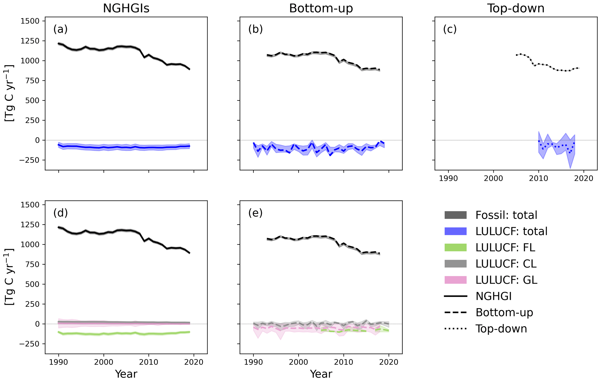
Figure 1 A synthesis of all the CO₂ net fluxes shown in this work for the EU27+UK. The estimates are divided by approach: NGHGI estimates (a, d), bottom-up methods (b, e), and top-down methods (c). Panels (d) and (e) include a breakdown of the (bottom-up) LULUCF flux into three of the dominant components: FL, GL, and CL. Such a breakdown is not provided for NGHGI CO₂ fossil as partitioning of bottom-up CO₂ fossil datasets corresponding to UNFCCC NGHGI categories is not currently available. The NGHGI UNFCCC uncertainty is calculated for submission year 2021 as the relative error of the NGHGI value, computed with the 95 % confidence interval method gap-filled and provided for every year of the time series, except for FL, GL, and CL, which are taken directly from the EU NIR (2021). Shaded areas for the other estimates represent the 0th–100th percentiles for groups with fewer than seven members and the 25th–75th percentile for groups with seven or more members. Ensembles (e.g., TRENDY v10) are included in the above only for their mean values to avoid more heavily weighting the ensembles compared to the other datasets.

Several caveats remain with this overall synthesis. First, the time series were combined rather naively in Fig. 1 by taking the mean of annual time series for each dataset discussed below. This leads to, for example, the 15-member TRENDY ensemble being given identical weight as the ORCHIDEE high-resolution simulation over Europe. This was done to weigh more heavily the regional approaches under the assumption that higher-resolution simulations and more region-specific input data will lead to more accurate results. While the latter assumption appears reasonable, the first assumption can be disputed. Finer resolution leads to models being exposed to values of input variables (e.g., temperature, rainfall) outside the parameterization range, which may result in unexpected behavior. Process representation can also change with spatial scale. Constant tree mortality, for example, is often used in models at coarse resolution, while abrupt tree mortality (stand-replacing disturbances) may better describe stand-level dynamics. Second, only a single top-down result for fossil CO₂ emissions is currently available, preventing an estimate of the uncertainty for this approach. Third, categorical models were combined by disregarding distinctions between those models estimating “Remain” and “Total” fluxes, where Total indicates all land of a particular type (e.g., Forest Land) regardless of the length of time it has been this type, i.e., Total is the sum of all Remain and Convert (see Table A1). These points are discussed in more detail in the following sections. However, addressing these points is highly unlikely to alter the overall conclusions in this section.

3.2 CO₂ fossil emissions

The inventory-based fossil CO₂ estimates from nine data sources (and some subsets) are presented as time series (1990 to the last available year) based on Andrew (2020) with the objective to explore differences between datasets and visualize trends (Fig. 2). Because the emissions source coverage (also called the “system boundary”) of datasets varies, comparing total emissions from these datasets is not a like-for-like comparison. Therefore, some harmonization of system boundaries prior to comparison is needed. This harmonization relies on specifying the system boundary of each dataset and, where possible, removing emission sources to produce a near-common system boundary. For example, IEA does not include any carbonates; thus, carbonates were removed from all emissions datasets that include them. UNFCCC (CRFs) Energy+IPPU, CDIAC, CEDS, PRIMAP, and GCP include the Energy sector plus all fossil fuels in IPPU; EIA, EDGAR, and BP include some fossil fuels in IPPU; and EIA and BP include bunker fuels as well. UNFCCC CRFs include Energy total and Energy combustion. Further details on how datasets are harmonized are provided by Andrew (2020). Because of differing levels of detail provided by datasets, it is not possible to do this perfectly, but the approximate harmonization gives something closer to a like-for-like comparison, with the legend in Fig. 2 indicating the most significant remaining differences. The pre-harmonization curves are shown in Appendix A3 (Fig. A1) for reference.

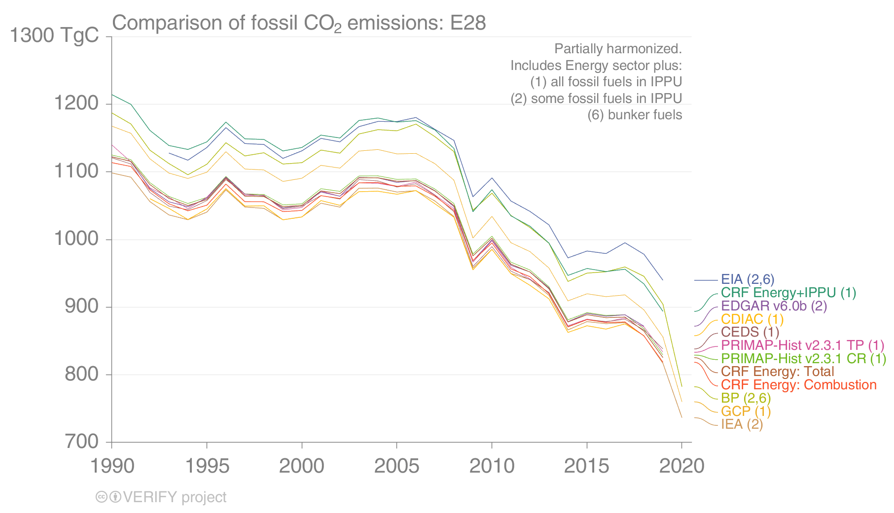
Figure 2 Comparison of the EU27+UK fossil CO₂ emissions from multiple inventory datasets with system boundaries harmonized as much as possible. Harmonization is limited by the disaggregated information presented by each dataset. CDIAC does not report emissions prior to 1992 for former Soviet Union countries. CRF: UNFCCC NGHGI from the common reporting format tables. The pre-harmonization figure is shown in Fig. A1.

Given the remaining differences in system boundaries after harmonization, most datasets agree well (Andrew, 2020). In response to inconsistencies identified in this work, the EIA recently corrected some double counting of emissions from liquid fuels and has revised its estimates of total emissions down about 10 % for the EU27+UK (US Energy Information Agency, personal communication, February 2022). For comparison, applying a similar harmonization procedure to the UNFCCC NGHGI and retaining only Fuel combustion (1A), Fugitive emissions (1B), Chemical industry (2B), Metal industry (2C), Non-energy products from fuels and solvent use (2D), and Other (2H) (see “Subsector” in Table A1) results in emissions of 930 ± 10 Tg C yr⁻¹ for the year 2017, where the uncertainty was propagated through quadrature using the gap-filled uncertainties described in this work and taking the total sector uncertainty if the category uncertainty was not available. This mean value falls within the 25th–75th percentiles of the eight other harmonized BU sources ([884,928] Tg C yr⁻¹). Across the overlapping time series, the mean value of the 25th–75th percentile is 24 Tg C yr⁻¹, with a 0th–100th percentile of 100 Tg C yr⁻¹.

The sole available inversion for CO₂ fossil fluxes is produced by the CIF-CHIMERE model, shown in Figs. 1c and B3 (for a single year). The inversion yields plausible fossil emission estimates, although it is below NGHGI estimates including both Energy and IPPU (Figs. 1a, c, B3) as well as the ensemble of nine bottom-up inventories. Uncertainties of the CIF-CHIMERE inversion estimate have not yet been quantified; however, they are likely largely driven by large uncertainties in the input data. The satellite observations of NO₂ have large uncertainties, which partly explains the small departure from the prior fluxes during the optimization. Emission ratios between NO_x and CO₂ are also uncertain (those from the prior are currently used). The atmospheric chemistry surrounding both production and destruction of NO₂ is another major source of uncertainty. The inversion reports total fossil CO₂ emissions calculated from NO_x fossil fuel combustion emissions. However, in principle, the derivation of CO₂ emissions from the NO_x inversions should be restricted to derivation of fossil fuel CO₂ emissions based on the fossil fuel CO₂ $/$ NO_x ratio from the TNO inventory, since there is no process linking the other fossil CO₂ emissions to the NO_x fossil fuel emissions. Future inversions co-assimilating CO₂ data will have to make a clearer distinction in the processing of fossil fuel and other anthropogenic emissions in order to exploit the joint fossil fuel signals in CO₂ and NO₂ observations. Finally, it is important to note that the inversion results are not fully independent of the bottom-up methods, as the prior estimates and CO₂ $/$ NO_x emission ratios are based on TNO gridded products. However, part of the lack of departure from the prior can also be attributed to the general consistency between the prior and the observations, which raise optimistic perspectives for the co-assimilation of co-emitted species with the data from future CO₂ networks dedicated to anthropogenic emissions.

3.3 CO₂ land fluxes

This section updates the benchmark data collection of CO₂ emissions and removals from the LULUCF sector in the EU27+UK previously published in Petrescu et al. (2020, 2021), expanding on the scope of those studies by adding additional datasets and years. The following graphs occasionally show large differences compared to previously reported values. This may happen when the model has undergone substantial changes since the work of Petrescu et al. (2021), such as the case with ORCHIDEE and the addition of a dynamic nitrogen cycle coupled to the carbon cycle. Such cases are both identified in the text as appropriate as well as in Table 2. The countries analyzed in this study use country-specific activity data and emission factors for the most important land use categories and pools (EU NIR, 2022; UK NIR, 2022). However, several gaps still exist, mainly in non-forest lands and non-biomass pools (e.g., soil carbon in Forest Land mineral soils and dead organic matter on Cropland and Grassland; for more details, see Table 6.6 in EU NIR, 2021). In addition, since NGHGIs largely rely on periodic forest inventories (carried out every 5 to 10 years) for the most important land use (Forest Land), the net CO₂ LULUCF flux often does not capture the most recent changes nor the full interannual variability.

While the net LULUCF CO₂ flux was relatively stable from 1990 to 2016, staying mostly between −80 to −95 Tg C yr⁻¹, in the past 3 years the sink has weakened to around −70 Tg C yr⁻¹ in 2020 (dotted black line in Fig. B2, Appendix B1; Raul Abad-Viñas, personal communication, 2022). This weakening occurred mostly in Forest Land, due to a combination of increased natural disturbances, forest aging, and increased wood demand (Nabuurs et al., 2013; EU NIR, 2022). Natural disturbances, including fires (especially in the southern Mediterranean), windthrows, droughts, and insect infestations (especially in central and northern European countries), have increased in recent years (e.g., Seidl et al., 2014), which explains most of the interannual variability of the NGHGI. Forest aging affects the net sink both through the forest growth (net increment) – which tends to level off or decline after a certain age – and the harvest, because a greater area of forest reaches forest maturity (Grassi et al., 2018b). Although the exact increase in total harvest in Europe in recent years is still subject to debate (Ceccherini et al., 2020; Palahí et al., 2021), demand for fuelwood at least has increased (Camia et al., 2020). The impacts of aging on mortality, another process which affects the net sink through reduced production and increased respiration, are less clear (e.g., Gray et al., 2016; Senf et al., 2018).

Net carbon uptake as seen by the atmosphere may occur on either managed or unmanaged land and results from the balance of processes such as photosynthesis, respiration, and disturbances (e.g., fire, pests, harvest). As discussed by Petrescu et al. (2020), the fluxes reported in NGHGIs relate to emissions and removals from direct LULUCF activities (clearing of vegetation for agricultural purposes, regrowth after agricultural abandonment, wood harvesting, and recovery after harvest, and management) but also indirect CO₂ fluxes due to processes such as responses to environmental drivers on managed land (e.g., long-term changes in CO₂, air temperature, and water availability). Additional CO₂ fluxes occur on unmanaged land, but the fraction of unmanaged land in the European Union is only around 5 % and divided between Forest Land, Grassland, and Wetlands. According to Table 4.1 in the EU27 and UK NIR (2022) CRF, almost all land (∼ 95 %) in the EU27+UK is considered managed. France and Greece report some unmanaged Forest Land (1.1 % and 16.6 %, respectively). Hungary and Malta report unmanaged Grassland of 33 % and 100 %, respectively; and Nordic and Baltic countries plus Ireland, Slovakia, and Romania report sometimes quite large (up to 100 %) unmanaged Wetlands.

The indirect CO₂ fluxes on managed and unmanaged land due to changing climate, increasing atmospheric carbon dioxide mole fractions, and nitrogen deposition are part of the (natural) land sink in the definition used in IPCC assessment reports and the Global Carbon Project's annual global carbon budget (Friedlingstein et al., 2022), while the direct LULUCF fluxes are termed “net land use change flux”, as discussed by Grassi et al. (2018a, 2021, 2022), Petrescu et al. (2020, 2021b), and Pongratz et al. (2021). Results should thus be interpreted with caution due to these definitional differences, but as most of the land in Europe is managed and the indirect effects are small, the definitional differences should be modest compared to other sources of uncertainty (Petrescu et al., 2020). Other relatively recent studies have already analyzed the European land carbon budget using GHG budgets from fluxes, inventories, and inversions (Luyssaert et al., 2012) as well as from forest inventories (Pilli et al., 2017; Nabuurs et al., 2018).

3.3.1 Estimates of CO₂ land fluxes from bottom-up approaches

In this section we present annual total net CO₂ land emissions between 1990–2020, i.e., induced by both LULUCF and natural processes (e.g., environmental changes) from category-specific models as well as from models that simulate multiple land cover/land use categories. The definitions of the categories may differ from the IPCC definitions of LULUCF (e.g., FL, CL, GL) where, according to IPCC (2006) guidelines, to become accountable in the NGHGI under “remaining” categories, a land use type must be in that category for at least N years (where N is the length of the transition period; 20 years by default). In an effort to create the most accurate comparison possible in terms of categories and processes included, total Forest Land (FL) has been divided up into Forest Land Remaining Forest Land (FL-FL) and land converted to Forest Land (X-FL), while only total Grassland (GL) and Cropland (CL) are reported. This is largely due to the non-forest categorical models explored here only considering net land use change, which prevents separating out the “converted” component.

3.3.2 Bottom-up estimates of CO₂ from Forest Land

Fluxes from Forest Land which remain in this category (FL-FL) are shown in Fig. 3 (top). These fluxes were simulated with ecosystem models (CBM and EFISCEN-Space, described in more detail in the Appendices) and countries' official inventory statistics reported to the UNFCCC. The results show that the differences between models are systematic, with CBM having slightly weaker sinks than EFISCEN-Space. CBM updated its historical data (1990–2015) and presents new NBP estimates based on extrapolation of historical time series (see Appendix A4) for 2017–2020 (CBMsim). Both CBM and EFISCEN-Space use national forest inventory (NFI) data as the main source of input to describe the current structure and composition of European forests. NFIs are also the main source of input data for most countries in the EU27+UK for NGHGIs (EU NIR, 2021), including data for carbon stock changes in various pools as well as the estimation of forest areas. Given that EFISCEN-Space does not cover all countries in the EU27+UK (Austria, Bulgaria, Denmark, Hungary, Lithuania, Portugal, and Slovenia are missing), the results were scaled by $\mathrm{1}/\mathrm{0.74}$ to account for the fact that the available countries comprise around 74 % of the forest NBP for the EU27+UK, according to previous EFISCEN results (Petrescu et al., 2021). As noted above, EU regulations are driving member states to report spatially explicit NGHGIs. Unlike the original EFISCEN, EFISCEN-Space is a spatially explicit model, in addition to being able to simulate a wider variety of stand structures, species mixtures and management options. Note that EFISCEN-Space reports only a single mean value for forest fluxes from 2005–2020; the annually varying value shown in Fig. 3 (top) arises from scaling by annually varying forest areas.

The bottom panel in Fig. 3 presents CO₂ land estimates for total Forest Land (FL, including both Remain and Convert classes). For the total Forest Land, the results were simulated with an ecosystem model (ORCHIDEE) and a global dataset (FAOSTAT) as it is not possible for these two approaches to separate out the “Remain” and “Convert” land use category. This obstacle arises due to the use of net land use/land cover information which does not include detailed information on the nature of the conversions. Consequently, Fig. 3 (bottom) compares flux estimates to those on all Forest Land from the countries' official inventory statistics (NGHGI, 2021).

The top and bottom panels in Fig. 3 are not directly comparable due to different quantities being displayed (FL-FL vs. FL). For the NGHGI, the value in the bottom panel is simply the value from the top panel with the addition of emissions/removals on land converted to Forest Land within the past 20 years. The sink gets stronger by around 20 Tg C yr⁻¹ when considering FL, which is to be expected as abandonment of Cropland or Grassland and subsequent regrowth of forest results in a net uptake of carbon due to storage in woody biomass. The UNFCCC NGHGI uncertainty of CO₂ estimates from Forest Land across the EU27+UK, computed with the error propagation method (95 % confidence interval; see IPCC, 2006), is 13.5 % for the year 2019 (EU NIR, 2021). This percentage is applied across all years for both FL and FL-FL, and in year 2019 it translates into an uncertainty of 12 Tg C for FL-FL.

Differences within the top panel of Fig. 3 are small, perhaps because all three approaches (NGHGI, CBM, EFISCEN-Space) rely heavily on forest inventory statistics. The same can be said for FAOSTAT FL fluxes in the bottom panel of Fig. 3. Among all the data plotted on the two graphs, ORCHIDEE stands out. Despite site-level evaluation (e.g., Vuichard et al., 2019), the vegetation classes in ORCHIDEE are fairly broad (e.g., temperate needleleaf evergreen) and parameterized to reproduce global fluxes, which means ORCHIDEE may be less suitable for regional simulations without further adjustments. As trends in forest carbon strongly result from management, the lack of explicit management in this version of ORCHIDEE also likely contributes, given the importance of management across Europe.

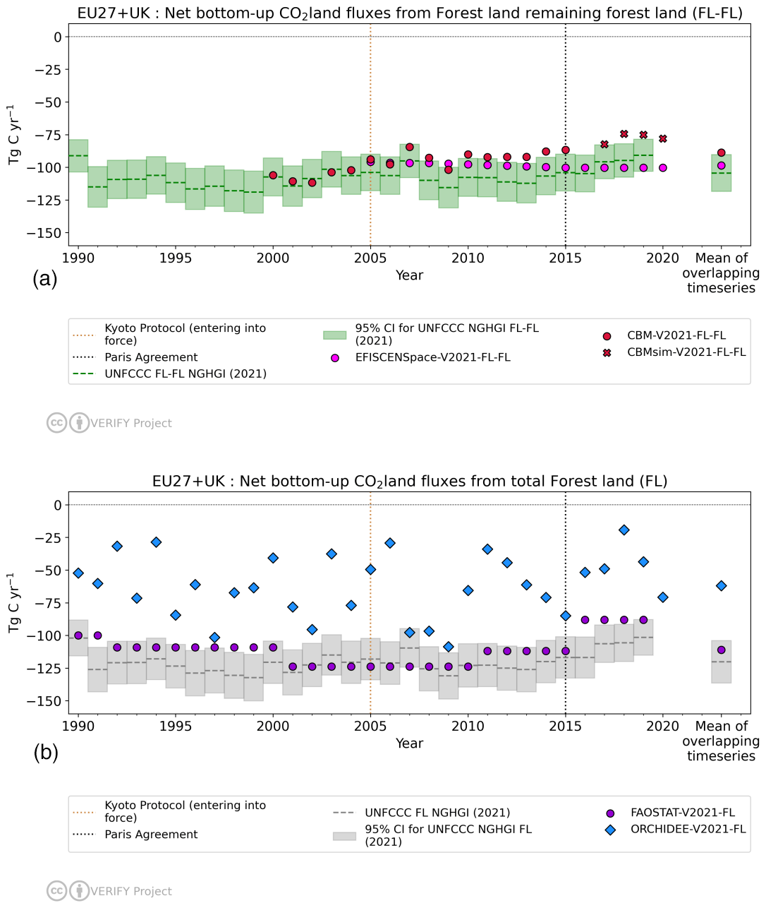
Figure 3 Net CO₂ land flux from Forest Land Remaining Forest Land (FL-FL, a) and total Forest Land (FL, b) for the EU27+UK. Means are given for 2005–2019 (a) and 1990–2019 (b) on the right side of both plots. CBM FL-FL historical estimates include 25 EU and UK countries (excluding Cyprus and Malta), in addition to new estimates for 2017–2020 (red crosses). EFISCEN-Space results have been scaled up from available countries as described in the text. FAOSTAT data do not include Romanian inventory estimates. The relative error on the UNFCCC value represents the UNFCCC NGHGI (2021) member state (MS)-reported uncertainty with no gap-filling, defined here as the 95 % confidence interval (CI) (EU NIR, 2021). The fluxes follow the atmospheric convention, where negative values represent a sink, while positive values represent a source.

Romanian estimates for FL in FAOSTAT (Fig. 3, bottom) have been removed due to a reporting inconsistency, which had not yet been corrected at the time of this analysis. In general, FAOSTAT results match well the NGHGI results, despite differences in models and even occasionally underlying data reported by countries to both organizations (Tubiello et al., 2021). ORCHIDEE was updated to include a dynamic nitrogen cycle coupled to the carbon cycle in this work. As shown in Appendix A4, the coupled nitrogen cycle results in a stronger sink, even if identical forcing is used. ORCHIDEE shows a higher interannual variability in carbon fluxes for forests than the NGHGI in Fig. 3 (bottom) because it incorporates meteorological data at sub-monthly timescales, while methods based on forest inventories are generally updated only every few years (e.g., 5 years for FRA), which results in a more climatological perspective. ORCHIDEE results indicate that climatic perturbations and extreme events (multi-month droughts, in particular) can have significant impacts on the net carbon fluxes depending on their timing in relation to the growing season. Flux tower measurements show that carbon sink strength in a European forest may weaken by 50 % during a summer drought, i.e., a loss of 15 % of net carbon uptake over the course of the year (Ciais et al., 2005). This is also to some extent supported by dendrometer data, although such data vary greatly among sites and tree species, which obscures a significant net effect (Scharnweber et al., 2020). It should also be noted that dendrometer data measure carbon stored in individual trees, while the NBP reported in figures in this paper includes respiratory fluxes from litter and soil. The variability of the weather affects the carbon dynamics of all components of the ecosystems (hence NBP), which, for instance, impacts on carbon assimilation rates, length of the growing season, dynamics of respiration rates, and allocation of the carbon in the plant (cf. Figs. 1 and 2 in Reichstein et al., 2013, and Bastos et al., 2020b).

3.3.3 Bottom-up estimates of CO₂ from Cropland and Grassland

Cropland (CL, UNFCCC subsector 4B) and Grassland (GL, UNFCCC sector 4C) include net CO₂ emissions from or removals by soil organic carbon (SOC) under “Remain” and “Convert” categories, and they are shown in the top and bottom panels of Fig. 4, respectively, for the EU27+UK along with four other approaches: one bottom-up inventory (FAOSTAT), two category-specific models (EPIC-IIASA, ECOSSE), and one DGVM (ORCHIDEE). The previous synthesis of Petrescu et al. (2021) compared models against NGHGI results for CL-CL and GL-GL. For the current work, we compare against the total Cropland (CL) and Grassland (GL) values. The reason for this is that FAOSTAT, ECOSSE, EPIC-IIASA, and ORCHIDEE all use land use/land cover maps generated by approach 1 in IPCC (2006), which only records the total amount of land in a category for each year; information on transitions between categories is unknown. Therefore, it is not possible to separate out “Remain” and “Convert” categories.

For CL during the common period (1990–2019), ORCHIDEE simulates a mean sink of −26 Tg C yr⁻¹, while ECOSSE, EPIC-IIASA, and FAOSTAT all simulate mean sources of 21, 10, and 16 Tg C yr⁻¹, respectively. With the exception of ORCHIDEE, all models are in line with the NGHGI results (22 ± 14 Tg C yr⁻¹). The sink in ORCHIDEE arises from the soil, as no simulated biomass in croplands remains from year to year; carbon is assimilated into biomass growth during the growing season, after which the biomass dies, is partitioned between litter and harvest (50 % to each), or either decays or vaporizes. In other words, no woody or perennial crops are simulated. Given more favorable growing conditions due to climatic changes and CO₂ fertilization, increased litter leads to more carbon entering the soil in ORCHIDEE in recent decades, which is driving the calculated CL sink observed in the model.

In the NGHGI, the reported source for the EU27+UK is mostly attributed to emissions from Cropland on organic soils⁹ in the northern part of Europe where CO₂ is emitted due to carbon oxidation from tillage activities and drainage of peat. In general, annual crops are assumed to be in carbon balance: any carbon assimilated during the year is respired in the same location. Woody crops (e.g., apple or olive orchards), however, are an exception, and Cropland on mineral soils uptake carbon in both France and Spain. Romania reports a strong sink on Cropland due to the inclusion of some forest plantations. Overall, emissions from organic soils on land converted to cropland dominate, however. Despite accounting for only 9 % of total Cropland area in the EU27+UK, they are responsible for 73 % of Cropland emissions (EU NIR, 2021). The fact that FAOSTAT values are similar to the UNFCCC values points to the primary role of drained organic soils, as this is the only flux included for the FAOSTAT dataset in Fig. 4. Finland and Sweden are of particular importance, as they together account for more than half of the total area of organic soil in Europe. Organic soils are an important source of emissions when they are under management practices that disturb the organic matter stored in the soil. In general, the NGHGI emissions from these soils are reported using country-specific values when they represent an important source within the total budget of GHG emissions.

ORCHIDEE also shows a much larger year-to-year variation than EPIC-IIASA and ECOSSE. This is unlikely to be caused by model time steps (EPIC-IIASA and ECOSSE at daily, ORCHIDEE at half-hourly) as both EPIC-IIASA and ECOSSE use minimum and maximum temperatures during the course of the day as input not simply the mean daily temperature. Therefore, all three models should see similar extremes, and crop vegetation may simply be more sensitive to meteorological forcing in ORCHIDEE. FAOSTAT and NGHGIs are mostly insensitive to interannual variability as the estimations are mainly based on statistical data for surfaces/activities and emission factors that do not vary with changing environmental conditions.

Both ECOSSE and EPIC show a striking improvement in agreement with the NGHGI between V2019 (Fig. B5, top) and the current work (Fig. B5, bottom). For ECOSSE, this is the result of improved data, in particular around residue management using the external tool MIAMI and more realistic fertilizer data (Mueller et al., 2012). For EPIC, the shifts in net CO₂ fluxes in the current EPIC results stem from the updated soil organic carbon and nitrogen module (Balkovič et al., 2020) and updates in meteorological forcing. Firstly, the updated soil module resulted in higher heterotrophic respiration across many EU regions. Besides attributing more carbon to the soil surface emissions, enhanced respiration leads to higher net primary production (NPP) and yields in regions with low fertilization rates as more nitrogen as is released from the soil organic matter (SOM) pool. Secondly, altered solar radiation and air temperature data affected the full range of carbon variables in EPIC, including NPP, harvested biomass, heterotrophic respiration, and leached carbon.

ORCHIDEE, EPIC-IIASA, and ECOSSE have previously been compared to measurements of net carbon fluxes and soil organic carbon changes at the site level (e.g., Balkovič et al., 2020; Chen et al., 2019; Zhang et al., 2018; Vuichard et al., 2019). Further comparison is outside the scope of this work, given site heterogeneities and the challenges in upscaling such data to a regional level as presented here. We note that this version of ORCHIDEE only includes management implicitly, which makes direct comparison to specific sites less informative.

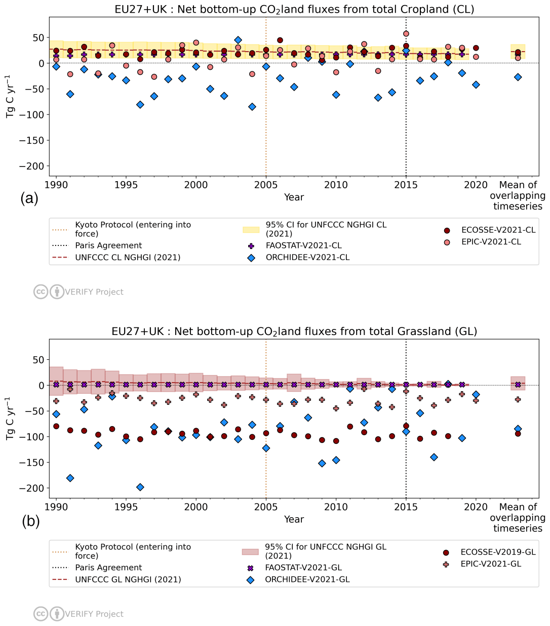
Figure 4 Net CO₂ land flux from total Cropland (a) and total Grassland (b) estimates for the EU27+UK. Total Cropland (CL) data come from the UNFCCC NGHGI (2021) submissions; ORCHIDEE, ECOSSE, and EPIC-IIASA process-based models; and the FAOSTAT inventory. Total Grassland (GL) data come from the same sources, with the caveat that ECOSSE has not been updated and is therefore identical to Petrescu et al. (2021). Values on the far right in both plots indicate the mean of 1990–2019. The relative error on the UNFCCC value represents the UNFCCC NGHGI (2021) MS-reported uncertainty with no gap filling (EU NIR, 2021). The fluxes follow the atmospheric convention, where negative values represent a sink, while positive values represent a source.

Differences between mean values may also arise from definitions for each land type, which vary between member states (see Tables 6.18 and 6.22 for Cropland and Grassland, respectively, in EU NIR, 2021). Woody and annual crops are included in NGHGI Cropland, although annual crops are generally assumed to be in carbon balance and thus to not contribute to the net flux. This also means that no spatial displacement of emissions (“lateral fluxes”) due to crop trade are taken into account. Grassland includes rangeland and pastureland which is not classified as Cropland. Urban green spaces, on the other hand, are often included in the Settlements category (EU NIR, 2021), which is not explicitly simulated by any bottom-up model reported here.

For Grassland, the NGHGI reports a slightly positive net flux over 1990–2019, although with a much larger uncertainty than for either Forest Land or Cropland (4 ± 13 Tg C yr⁻¹). While increased uncertainty compared to Forest Land emissions is understandable given the emphasis on collecting accurate forestry statistics due to their economic importance, the increased uncertainty in Grassland compared to Cropland is more puzzling. Uncertainty estimates for the EU27+UK come from a synthesis of estimates for each of the 28 member states and are applied to each year individually based on the data provided for a single year (2019). The apparent drastic change in uncertainty from 1990 to 2019 is due to the emissions getting much closer to zero (i.e., 7.8 Tg in 1990 compared to 0.5 Tg in 2019), which itself is due primarily to changes in the way Grassland is treated in the United Kingdom, Bulgaria, and Sweden (EU NIR, 2021). Additional analysis will be needed to elucidate this issue.

In addition to the NGHGI, updated results for GL are available for ORCHIDEE (using a coupled C–N cycle) and FAOSTAT. For the first time, EPIC-IIASA contributed estimates for Grassland fluxes using five different grassland types and simulating carbon export due to herbivores (see Appendix A4 for more details). Both of these models exhibit a strong sink in Grassland. For ORCHIDEE, this is likely due to the same reasons as the sink in croplands: more suitable growing conditions due to climate change, CO₂ fertilization, and nitrogen deposition leading to increased inputs into the soil which are not lost during tillage due to the lack of explicit management in the version reported here. For EPIC-IIASA, this results from manure left on site and incorporated into the soil. A Tier 1 IPCC approach, used in both the FAOSTAT inventory and many NGHGIs in the EU27+UK, assumes no changes in either living or dead biomass pools on Grassland. In addition, it only considers organic soils which have been drained for grazing, and it only considers mineral soils which have undergone a change in management. This greatly reduces or eliminates mechanisms which promote sinks in ORCHIDEE and EPIC-IIASA. On the other hand, FAOSTAT reports a slight source in Grasslands, in line with the NGHGI. This is because, as is the case for Cropland, FAOSTAT data only consider emissions from drained organic soils. As incorporation of manure in EPIC-IIASA changes grasslands from a net source to a net sink, consideration of CO₂ from manure input in other inventories may have a similar effect.

3.3.4 Total bottom-up and top-down LULUCF CO₂ estimates

This section analyzes CO₂ emissions and sinks for the LULUCF sector, including NGHGI categories (from Fig. B4) and a suite of different bottom-up and top-down approaches. This comparison is challenging due to differences in terms of activities covered in the different estimates, as well as differences in terminology (see, for example, Petrescu et al., 2020, Fig. 12, and Petrescu et al., 2021, Sect. 3.3.4). Given the differences noted in those references, the comparison in this section should be considered a rough overview that highlights both important aspects of the carbon cycle and questions that need to be addressed in the future. Going towards a more specific comparison of only net land use change (LUC) fluxes would require additional considerations. In GCP's annual global carbon budget, the net LUC term is estimated by global DGVMs as the difference between a run with and a run without land use change (i.e., the S3 and S2 simulations from TRENDY, respectively) and by bookkeeping models (Friedlingstein et al., 2022). Such an estimate is given in Fig. 13 in Petrescu et al. (2020) for Forest Land. However, even taking S3–S2 does not permit an apples-to-apples comparison between DGVMs, bottom-up inventories, and bookkeeping models. In particular, questions remain about net vs. gross land use change, managed vs. unmanaged land, and emissions from wood harvest. In addition, UNFCCC “convert” emissions (i.e., emissions resulting from land that has been converted from one type to another) are reported within 20 years following conversion in the “convert” category (biomass losses are typically reported in the year of conversion, while net changes in soil organic carbon are reported during the entire conversion period). FAOSTAT, DGVMs, and bookkeeping models usually only include “convert” fluxes from the year following conversion, although bookkeeping models and DGVMs which deal with gross transitions may be able to include this transition period more easily.

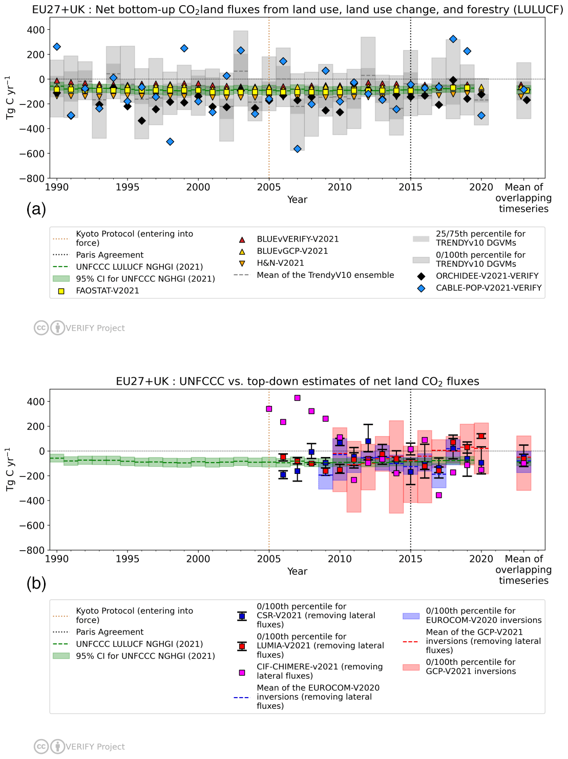
Figure 5 Net CO₂ fluxes from total LULUCF activities in the EU27+UK from bottom-up (a) and top-down (b) methods compared to the UNFCCC NGHGI (2021). The bottom-up methods include BLUE-vVERIFY, BLUE-vGCB, H&N (GCB2021), DGVMs (TRENDY v10), and FAO (2021), as well as ORCHIDEE and CABLE-POP with high-spatial-resolution (0.125^∘) meteorological forcing (both models are also part of the TRENDY ensemble at 0.5^∘). The spread of the gray bars represents the individual model data for the DGVMs. Top-down inversion results are the global GCB2021 ensemble, as well as several regional inversions: the EUROCOM ensemble, the CarboScopeReg model with multiple variants, the LUMIA model with multiple variants, and CIF-CHIMERE. The colored area represents the min/max of top-down model ensemble estimates. Emissions due to lateral fluxes of carbon through rivers, crop trade, and wood trade are removed from the top-down estimates. The mean values of the time series for the overlapping periods of 1990–2019 (a) and 2010–2018 (b) are shown on the right. The UNFCCC estimate includes all categories (Remain and Convert), as well as HWP. The relative error of the UNFCCC values represent the UNFCCC NGHGI (2021) member-state-reported uncertainty computed with the error propagation method (95 % confidence interval), gap-filled, and provided for each year of the time series. The fluxes follow the atmospheric convention, where negative values represent a sink, while positive values represent a source.

Figure 5 (top) shows CO₂ fluxes from the NGHGI LULUCF sector compared to all other comparable bottom-up (BU) estimates in this work: high-resolution S3 simulations for both ORCHIDEE and CABLE-POP, the median of 15 S3 simulations from the TRENDYv10 DGVM ensemble, three bookkeeping models, and FAOSTAT. As mentioned above, taking the difference of the TRENDY S2 and S3 simulations does not permit a fully consistent comparison between DGVMs, bottom-up inventories, and bookkeeping models for LULUCF fluxes, and for simplicity we simply report S3 NBP from DGVMs in Fig. 5. Further research is needed in order to establish which approach (S3–S2, or simply S3) leads to the most consistent comparison. For the overlapping period 1990–2019, the means of two out of the three bookkeeping models (BLUE-vGCB (−61 Tg C yr⁻¹) and BLUE-vVERIFY (−43 Tg C yr⁻¹, using the Hilda+ land use forcing)) along with the mean of FAOSTAT (without Romanian forestry fluxes) (−93 Tg C yr⁻¹) fall within the 95 % confidence interval of the UNFCCC NGHGI estimate of −86 ± 33 Tg C yr⁻¹. Only H&N rests apart with a stronger sink (−142 Tg C yr⁻¹), although it is difficult to say how different it is from the NGHGI without uncertainty estimates.

Bookkeeping models like BLUE and H&N always regrow biomass at the same rate. In the bookkeeping approaches used here, regrowth curves are representative for present-day conditions and kept the same throughout history, which is the same approach used in the global carbon budget. NGHGIs, on the other hand, include legacy effects from changing environmental conditions, in particular in soil pools. Recent work by Grassi et al. (2023) demonstrates that including the sink associated with varying human-induced indirect effects (as estimated by the S2 simulations from the TRENDY DGVM ensemble) into results by bookkeeping models can largely reconcile estimates of net global LULUCF fluxes between the NGHGIs and bookkeeping models. At the level of the EU27+UK, the inclusion of this sink results in an overcompensation; the bookkeeping models estimate a net sink of −56 Tg C yr⁻¹ compared to the NGHGI estimate of −88 Tg C yr⁻¹, while the bookkeeping models plus DGVMs result in −112 Tg C yr⁻¹. However, both of these estimates fall inside the NGHGI uncertainty range in Fig. 5.

The primary difference between the NGHGI and DGVMs is the interannual variability, with only a small difference in the means even if there is a substantial amount of spread with the DGVMs: −86 ± 33 Tg C yr⁻¹ and −81 [$-\mathrm{172},-\mathrm{20}$] Tg C yr⁻¹ for the NGHGI and DGVMs, respectively, where the range for the DGVMs indicates the 25th–75th percentile of the models in the ensemble. The UNFCCC LULUCF estimates contain CO₂ emissions from all land use categories and HWP, where a simple analysis shows that for the EU27+UK almost 90 % of the gross flux arises from only six categories (Table A4). DGVMs currently explicitly include more of these categories than the other methods (Table C2), which may help explain the closeness between the mean values. ORCHIDEE and CABLE-POP provide a nice test case of the impact of high-spatial-resolution forcing on net carbon fluxes in the EU27+UK, as they are present in both the TRENDY ensemble (0.5^∘) as well as the VERIFY results (0.125^∘). Using 1σ of the mean annual net CO₂ flux as a measure of the IAV, CABLE-POP indeed shows a much higher IAV at high resolution (−40 ± 142 and −92 ± 214 Tg C yr⁻¹ for TRENDY and this work across 1990–2019), while the results for ORCHIDEE are almost identical between the two resolutions. More analysis is therefore required to confirm the relationship between spatial resolution and interannual variability in DGVMs for the EU27+UK.

The differences between bookkeeping models and UNFCCC and FAOSTAT are discussed in detail elsewhere and focus on the inclusion of unmanaged land in bookkeeping models but not FAOSTAT and UNFCCC methodologies (Petrescu et al., 2020; Grassi et al., 2018a, 2022). ORCHIDEE, CABLE-POP, and the TRENDY v10 ensemble means show much higher interannual variability as they simulate subannual responses of carbon fluxes to climate, while the climate responses of inventories and bookkeeping models are averaged over multiple years. A comparison including categorical-specific models (e.g., ECOSSE, EFISCEN-Space, EPIC-IIASA, CBM) where multiple model results are harmonized and aggregated to produce a “total” LULUCF flux comparable to DGVMs and bookkeeping models would be insightful; however, such a comparison requires extensive analysis which is beyond the scope of the current work.

The bottom panel in Fig. 5 highlights the range of estimates from global and regional atmospheric inversions (GCB2021, EUROCOM, CSR, LUMIA, and CIF-CHIMERE; see Table 2 and Appendix A4 for more details) against bottom-up total annual EU27+UK CO₂ land emissions/removals from the UNFCCC NGHGI (2021). Notice that unlike other studies (e.g., Deng et al., 2022), we have not applied a managed-land mask to the inversions or bottom-up models in order to be compatible with the managed land proxy in the NGHGIs. The reasons for this are twofold. One, most of the land in the European Union is managed, as noted above. Second, no such mask currently exists, even for the relatively data-rich EU. A managed land mask created solely based on non-intact forests (e.g., Deng et al., 2022) neglects that Grassland and Wetlands contribute significantly to unmanaged areas in the EU. Including fluxes from the 5 % of unmanaged land in the EU is unlikely to change any conclusions in this work given the uncertainties in the LULUCF methods presented here. As soon as a reasonably accurate managed land mask is available, however, it should be used.

One significant change between this work and Petrescu et al. (2021) is the removal of emissions and sinks from inversion results due to lateral transport of carbon from crop trade, wood trade, and inland waters. Bottom-up methods (including all the NGHGIs for European countries) do not consider emissions and removal of atmospheric CO₂ due to lateral transport of biomass carbon, while inversions calculate geographically resolved net land–atmosphere CO₂ fluxes without regard to the original location of photosynthetic assimilation. Some lateral transport of soil organic carbon may be taken into account by measuring stock changes, but given the mix of stock-change and gain–loss methods used in NGHGIs in the EU and the presence of methods ranging from Tier 1 to Tier 3, exactly how much is far from trivial to determine.

Net emissions from lateral transport of carbon (“lateral fluxes”) were prepared generally following the approach described by Ciais et al. (2021), where crop and wood product fluxes are derived from country-level trade statistics compiled by the FAO. Inland water emissions and riverine export of terrestrial carbon use spatially explicit climatological data and a statistical model combined with estimates of gas transfer velocities. A more complete description is given in Appendix A4. This adjustment accounts for a combined mean of −140 Tg C yr⁻¹ over the 2010–2018 common period of the inversions and has been applied using Eq. (1) in Deng et al. (2022) (without a managed land mask) to all top-down fluxes reported here unless indicated otherwise.

Uncertainties for net emissions of CO₂ due to lateral transport of carbon are not yet available. However, FAO and IEA statistics form the basis of calculated fluxes due to wood and crop trade. FAO estimates an uncertainty of 50 % on carbon emissions and removals from forested land (Tubiello et al., 2021). Even if uncertainties in trade fluxes are not available, 50 % therefore works as a first-order approximation given the similarities between the two fluxes (i.e., a well-tracked value multiplied by an uncertain emission factor). Uncertainties in net carbon uptake by rivers and lakes are estimated to also be on the order of 50 % due to the fact that these fluxes can only be calculated based on budget closure including estimates of river exports to the coast, emissions of carbon from the water surface to the atmosphere, and burial of carbon in aquatic sediments (Battin et al., 2023). Combined, this results in an uncertainty of around 70 Tg C yr⁻¹ for the lateral fluxes, which is on the same order as the ensemble spread for the regional inversions as shown in Fig. 5, though still lower than that of the global inversions.

Flux estimates from inversion methods for CO₂ land show much more variability than the NGHGI, both on the interannual scale, as well as for any given year (Fig. 5, bottom). The mean values from 2010–2018 show good agreement but with an order of magnitude more variability in the inversions: −88 ± 60 Tg C yr⁻¹ for EUROCOM and −80 ± 6 Tg C yr⁻¹ for the NGHGI, where the uncertainty here is the standard deviation of the annual mean values for each. For any given year, the spread between the inversions is also much greater (170 ± 70 Tg C yr⁻¹ for EUROCOM versus 63 ± 3 Tg C yr⁻¹ for the NGHGI, which represents the mean and standard deviation of the 0–100th percentiles for the inversions and the 95 % CI for the NGHGI). This large spread per year can be linked to uncertainty in atmospheric transport modeling, inversion methods and assumptions, and to limitations of the observation system. Furthermore, the EUROCOM inversions were designed for the European geographical domain (which is larger than the EU27+UK) and are still being developed in particular to better constrain the latitudinal and longitudinal boundary conditions.

The annual mean (overlapping period 2010–2018) of the EUROCOM v2021 inversions (−80 [$-\mathrm{175},-\mathrm{4}$] Tg C yr⁻¹) is the closest inversion estimate to the time series mean of the NGHGI estimates (−88 ± 31 Tg C yr⁻¹), where the error bars for the inversion indicate the [0th, 100th] percentiles due to the small size of the ensembles. The ensemble of all regional inversions is consistent with the NGHGI estimates, assuming the spread of the inverse model results is an accurate proxy of the structural uncertainties. The impact of the net emissions of lateral fluxes due to wood trade, crop trade, and rivers is clear: without factoring in their contribution of the approximately −140 Tg C yr⁻¹, the sink from regional inversions, in particular, would be much stronger than even the strongest estimate of the NGHGI (i.e., the lower boundary on the green bar in Fig. 5). The mean of the global GCP2021 inversions (−50 [$-\mathrm{320},+\mathrm{122}$] Tg C yr⁻¹) and regional inversions, CSR (−46 [$-\mathrm{126},+\mathrm{47}$] Tg C yr⁻¹) and LUMIA (−65 [$-\mathrm{97},-\mathrm{27}$] Tg C yr⁻¹), show a lower absolute value but report larger interannual variability (min/max). The new CIF-CHIMERE product has a mean of −99 Tg C yr⁻¹, showing a trend towards more negative fluxes since 2010, which is not seen in other models and is still under investigation.

The comparison of past and current versions of the inversions shows changes in specific top-down models (Fig. B5). A reduction in the spread of the estimates is noted over the two past versions of CSR, resulting in a small source in the most recent estimates. The CSRv2021 (bottom-plot) predicts in 2018 (last common year of both versions) a small source of 19 [$-\mathrm{64},+\mathrm{100}$] Tg C yr⁻¹ compared to the previous CSRv2019 which simulated a very strong sink of −253 [$-\mathrm{280},-\mathrm{194}$] Tg C yr⁻¹. This smaller source appears more in line with more positive fluxes expected in years of extreme drought (e.g., 2018 in northern Europe, even if this did not impact the whole EU27+UK; Toreti et al., 2019).

As can be seen in Fig. 5 (bottom), there is also improved agreement between the EUROCOM ensemble and the NGHGI, including a greatly reduced IAV compared to the previous version. The small EUROCOM ensemble mean sink for the 2009–2015 period of −1.9 [−335,+322] Tg C yr⁻¹ (top panel) strengthened to −93 [$-\mathrm{187},-\mathrm{15}$] Tg C yr⁻¹ in the v2021 version (bottom panel). The UNFCCC total LULUCF mean is −92 ± 33 Tg C yr⁻¹ for the same time period. The IAV of EUROCOM was dramatically reduced by removing the FLEXINVERT model from the v2021 ensemble as a clear outlier of annual means due to a slightly shifted seasonal cycle (Appendix A4).

Despite an apparent trend in the mean of the new GCB2021 inversions towards a source near 2017, the spread of the models precludes significance; following 1000 realizations of a Monte Carlo analysis assuming the min–max ensemble spread represents 3σ in a normal distribution, the only period of at least 4 consecutive years for which the 95 % confidence interval of the trend comes close to excluding zero is 2015–2018 (26 ± 28 Tg C yr⁻²). The large variability and high sink observed in the upper plot of Fig. 5 (bottom) shifted to a source in 2019 (21 [$-\mathrm{185},+\mathrm{226}$] Tg C yr⁻¹) due to the extreme climatic response of the TD models to the drought year, which can also be observed in the BU simulations (e.g., TRENDY v10, ORCHIDEE, and CABLE-POP in the top panel of Fig. 5). Out of the GCB2021 models, CAMS was the model responsible for the strongest sink in the ensemble during most years (data not shown), which may be partly due to changes in the stations assimilated.

3.4 Uncertainties in top-down and bottom-up estimates

Uncertainties are essential for complete comparisons between models and approaches. This section summarizes the main sources of uncertainty estimates interwoven throughout the above text. We also provide a comparison of available uncertainties between the previous synthesis (V2019) and the current synthesis (V2021) for both bottom-up and top-down methods. Finally, we give an overview of two important advances in uncertainty estimation included in this work (one for the NGHGI, and one for top-down approaches), referring the interested reader to Appendix A4 for more information.

Several sources of uncertainty arise from the synthesis of bottom-up (BU) inventories and models of carbon fluxes, which can be summarized as the following: (a) differences due to input data and structural/parametric uncertainty of models (Houghton et al., 2012) and (b) differences in definitions (Pongratz et al., 2014; Grassi et al., 2018b, 2022; Petrescu et al., 2020, 2021). Posterior uncertainties in top-down (TD) estimates mostly come from the following: (1) errors in the modeled atmospheric transport; (2) aggregation errors, i.e., errors arising from the way the flux variables are discretized in space and time and error correlations in time; (3) errors in the background mole fractions, in particular for regional inversions; and (4) incomplete information from the observations and hence the dependence on the prior fluxes. The multi-model ensemble approach is being used as a proxy for estimation of systematic error. Calculation of random error is generally difficult when using the most common inverse model flux optimization approaches.

Figure 6 summarizes the quantifiable uncertainties in this work, compared to previous results from Petrescu et al. (2021). With the exception of the NGHGI, all the other uncertainties are calculated from ensembles of simulations using either (1) multiple models of the same general type (either using model-specific inputs or attempting to harmonize inputs as much as possible, e.g., TRENDY) or (2) multiple simulations with the same model, varying input parameters and/or forcing data (e.g., CarboScopeRegional, LUMIA). As a complete characterization of model uncertainty involves exploring the full parameter, input data, and model structure space, none of the uncertainties reported here can be considered complete, but they represent best estimates given realistic constraints of resources and knowledge. The uncertainties represent the mean of overlapping periods for the previous V2019 (overlapping period: 2006–2015) versus the current V2021 (2010–2018). In general, the differences in mean behaviors between the two versions falls within uncertainty estimates. Note, however, that this graph can hide certain behaviors. For example, the similarity in the means for ORCHIDEE-VERIFY for both periods (−129 and −131 Tg C yr⁻¹ for V2019 and V2021, respectively) is likely a coincidence, given the wide fluctuation of annual values and the differences in the multi-decennial means seen in Fig. 5.

Figure 6 shows notable reductions in the spread of two ensembles: EUROCOM and CSR. Both of these are regional ensembles. In addition, the CSR results show a weaker sink in the current V2021 version compared to the previous V2019 version. As noted in Appendix A4, the change for CSR is explained by the inclusion of a corrected observation dataset for an isolated station in southeastern Europe which heavily influenced the regional results. The reduction in the spread of the EUROCOM ensemble results from the exclusion of a single member which produces annual flux results that are clear outliers compared to the remaining three members. More details of this analysis can be found in Appendix A4. The remaining ensembles retain similar model spread compared to the previous versions.

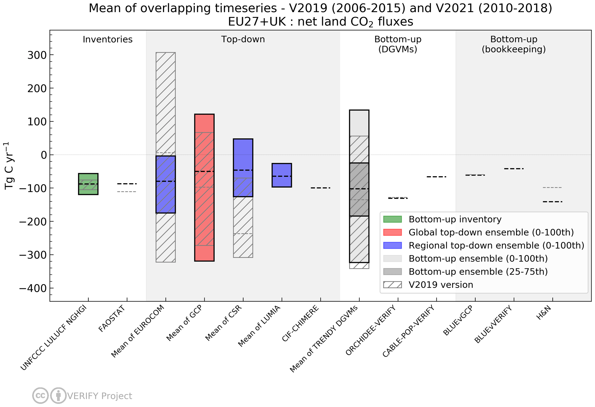
Figure 6 Mean annual values of overlapping time periods (2006–2015) from Petrescu et al. (2021b) (transparent boxes and light gray lines) and new means for the 2010–2018 period from the current study (Fig. 5, Sect. 3.3.4). The boxes with hatching and colored boxes depict the “old” and “new” values for ensembles of multiple models, with the top and bottom of the boxes corresponding to minimum and maximum mean values of the overlapping period. For non-ensemble models (e.g., CIF-CHIMERE, FAOSTAT), the mean of the old and new overlapping periods are given by dotted gray and dashed black lines, respectively. The NGHGI UNFCCC uncertainty is calculated for submission year 2021 as the relative error of the NGHGI value, computed with the 95 % confidence interval method gap-filled and provided for every year of the time series. Inversions for both V2019 and V2021 have been corrected for net emissions of CO₂ from lateral transport of carbon using identical datasets to enable a fair comparison. The fluxes follow the atmospheric convention, where negative values represent a sink, while positive values represent a source.

Three advances in uncertainty estimation were made in this study, involving all three classes of models: NGHGI, bottom-up, and top-down models. In Petrescu et al. (2021b), percentage uncertainties for the NGHGI (2019) LULUCF sector and land use categories were taken from reported uncertainties of the EU member states and UK that are used for compiling the national inventory reports (NIRs) of the EU27+UK bloc, as well as the aggregate uncertainties for the block reported in the EU NIRs. Uncertainty estimates were only given for a single year and were also partially incomplete due to missing uncertainty estimates for some sectors/subsectors of some countries. For the current work, we use values compiled by the EU inventory team involving a recently developed procedure to harmonize and gap-fill uncertainties reported by the member states at the sector level (see EU NIR, 2021). Error correlations are accounted for, in addition to year-to-year variations in subsectoral contributions to the overall uncertainty. Extensive details are found in Appendix A2 and permit estimates of uncertainty on an annual basis, as opposed to the single value used in the previous synthesis. Note, however, that this procedure was not applied to subsectoral categories (FL, CL, or GL), for which values were taken directly from EU NIR (2021) and applied across the whole time series. Synthesis plots created for individual countries and reported on the VERIFY website (VERIFY Synthesis Plots, 2022) take percentages directly from the respective country's NIR.

The second advance relates to the impact of forcing data on bottom-up models, in particular DGVMs. Figure A3 (Appendix A4) shows how the ORCHIDEE model responds to both changes in meteorological forcing (for ORCHIDEE) and nitrogen forcing (for ORCHIDEE-N) over the past several decades. The impact of both is relatively small compared to interannual variability. This is likely due to at least two reasons. The first reason is that meteorological forcing used in this work has been realigned to the CRU observational dataset at 0.5^∘ and monthly resolution, thus removing large-scale and long-term differences between the original meteorological datasets. In addition, extensive spin-up and transient simulations are run for ORCHIDEE before reaching the point at which the forcing changes (1981 for the meteorological forcing, and 1995 for the nitrogen forcing). Such lengthy simulations enable woody biomass and soil carbon pools to develop a significant amount of inertia in response to additional changes. Greater differences may be seen for models where modified forcing data cover the entire length of the preproduction simulation steps.

The final advance relates to uncertainty characterization in the regional inversion model CSR following the methodology of Chevallier et al. (2007). Spatially explicit estimates of the uncertainty reduction achieved from the flux optimization were prepared through a Monte Carlo approach using an ensemble of 40 members. The uncertainty reduction is then calculated based on the ratio of the prior errors and the posterior spread of the ensemble members, using a formula such that 0 indicates no reduction and 1 indicates a complete elimination of uncertainty. A preliminary analysis showed that a considerable reduction may be achieved through the inclusion of more observation stations, although additional work is needed. For the moment, these maps only reflect random uncertainties, and systematic uncertainties remain poorly characterized. More information can be found in Appendix A4.

4 Data availability

Annual time series for the EU27+UK used in the creation of the figures in this work for V2019 and V2021 are publicly available for download at https://doi.org/10.5281/zenodo.8148461 (McGrath et al., 2023). This excludes CO₂ fossil data for the IEA, which is subject to license restrictions. Most sector-level data from IEA are available for a fee, although some high-level emissions data can be accessed free of charge. The data are reachable with one click (without the need for entering a login or password) and downloadable with a second click, consistent with the two-click access principle for data published in ESSD (Carlson and Oda, 2018). The data and the DOI number are subject to future updates and only refer to this version of the paper. In addition, figures and annual time series for the EU27+UK as well as other countries and regions are available from VERIFY Synthesis Plots (2022) as well as a number of gridded data files submitted to the VERIFY project listed in Table C1. Access to the data files requires free registration to obtain a username and password. Alternatively, interested users are invited to contact the persons listed in Table C1 to request gridded data files directly from them. We do not provide access to data already made freely available elsewhere, as we prefer users to use mechanisms put in place by the original providers so that they are able to ensure their continued funding for their work.

5 Summary and concluding remarks

This work represents an update to the Petrescu et al. (2021) European CO₂ synthesis paper, presenting and investigating differences between the UNFCCC NGHGI, BU data-based inventories, both coarse- and high-resolution process-based BU models, and TD approaches represented by both global and regional inversions. Datasets used in the previous work have been updated by extending the temporal coverage and updating the models and data behind the calculations. In addition, several new models to expand the number of independent approaches compared have been added. Additional efforts have been made to improve uncertainty characterization in two approaches, along with a first attempt to present as many datasets as possible in a clear single figure to draw overarching conclusions.

CO₂ fossil emissions dominate the anthropogenic CO₂ flux in the EU27+UK, regardless of the approach employed and irrespective of uncertainties, although the datasets are not fully independent, which complicates uncertainty estimation. Fossil CO₂ emissions are more straightforward to estimate than ecosystem fluxes due to extensive data collection around fuel production and trade, assuming that fuel statistics and accurate emission factors are available. A suite of eight BU methods for fossil CO₂ emissions are within the uncertainty of the NGHGI when methods are harmonized to include similar categories. The remaining differences can often be attributed to definitions, assumptions about activity data or emission factors, and the allocation of fuel types to different sectors (see Sect. 3.2 and Fig. B3). The one available TD method, a regional European inversion system (CIF-CHIMERE) using an NO_x proxy to determine CO₂ fossil emissions, shows broad agreement with the BU estimates. However, this initial TD inversion is not yet capable of distinguishing the minor differences between the various BU estimates and does not yet quantify uncertainties, unlike, for example, Basu et al. (2020), which presents fossil fuel combustion and cement production emission including uncertainty estimates for the United States. However, a substantial decrease in the level of uncertainty of the inverse modeling system is expected in the short term with the large-scale deployment of observation networks dedicated to detecting fossil fuel emissions (e.g., launch of the CO₂M¹⁰ satellite mission in 2025). In the short-term, the CoCO2 project (CoCO2, 2022) aims to advance the methodology around co-assimilation of existing CO₂ satellite data (from the Orbiting Carbon Observatory (OCO)-2/3 instruments) and to provide new analysis of the CO $/$ FFCO₂ and NO_x $/$ FFCO₂ ratios in order to significantly decrease uncertainty in the fossil CO₂ estimates.

The CO₂ land fluxes belong to the LULUCF sector, which is one of the most uncertain sectors in UNFCCC reporting. The IPCC guidelines prescribe methodologies that are used to estimate the CO₂ fluxes in the NGHGI but grant countries significant freedom to adopt methods appropriate to their national circumstances. Even in the European Union, member states use a wide variety of stock-change and gain–loss methods ranging from Tier 1 to Tier 3, depending on the specific LULUCF flux being estimated (EU NIR, 2021). When analyzing the different estimates from multiple BU sources (inventories and models), similar sources of uncertainties are observed such as the following: (a) differences due to input data and structural/parametric uncertainty of models (Houghton et al., 2012; Pongratz et al., 2021) and (b) differences in definitions (Pongratz et al., 2014; Grassi et al., 2018b; Petrescu et al., 2020, 2021; Grassi et al., 2022). Reducing uncertainties in LULUCF estimates is needed, given the increasing importance of the sector to EU climate policy over the next decades. In contrast to the previous 2020 climate and energy package, the LULUCF sector will now formally contribute to the binding emission reduction targets of the union's 2030 climate and energy framework (EU, 2018a, b). Furthermore, the European Climate Law explicitly states that LULUCF, together with all sectors of the economy, should contribute to achieving climate neutrality within the union by 2050 (EU, 2021b).

The LULUCF sector in NGHGIs is composed of six land use categories. Of these, Forest Land provides the most important contribution to the net CO₂ land flux in the EU27+UK, followed by Cropland and Grassland. HWP and “Land converted to settlements” also have non-negligible contributions, and changes in HWP strongly influence variations in decennial mean net LULUCF fluxes for the region. Of these, all except “Land converted to settlements” are represented in general ecosystem models, while Forest Land, Cropland, and Grassland are simulated by category-specific process-based and data-driven models. Top-down inversions are capable of simulating net CO₂ fluxes to the atmosphere but cannot yet attribute them between different categories.

Differences in the detailed category-specific and inversion model results (Figs. 3–5) often come from choices in the simulation setup and the type of model used: bookkeeping models, process-based DGVMs, inventory-based statistical methods, or atmospheric inversions. Results also differ based on whether fluxes are attributed to LULUCF emissions due to the cause or location of occurrence. For example, indirect fluxes resulting from long-term changes in growing conditions, such as CO₂, air temperature, and water availability on managed land, are included in NGHGIs and FAOSTAT. Additional sink capacity compared to pre-industrial conditions (also called the “amplification effect”, e.g., Gasser and Ciais, 2013) occurs on Forest Land in process-based models (e.g., ORCHIDEE or TRENDY DGVMs) due to improved growing conditions resulting from CO₂ fertilization, climate change, and anthropogenic nitrogen deposition, while this is not included in bookkeeping models which use the same regrowth curves for pre-industrial and modern times. The use of gross land use changes fluxes (e.g., in the NGHGI, bookkeeping models, and CABLE-POP) as opposed to net fluxes also likely plays an important role. We found that adjusting top-down models by emissions/removals resulting from later transport of carbon through trade and the inland water network improves the agreement with the NGHGI of the EU27+UK (Fig. 5, compared to Petrescu et al., 2021).

Observation-based BU estimates of LULUCF provide large year-to-year flux variability (Figs. 3–4, in particular for DGVMs like ORCHIDEE, CABLE-POP, and the TRENDY ensemble), contrary to the NGHGI, primarily due to the effect of varying meteorology. In particular, the duration and intensity of the summer growing season can vary significantly between years (e.g., Bastos et al., 2020a; Thompson et al., 2020). In the framework of periodic NGHGI assessments, the choice of a reference period (such as 2015–2019, as used here) or the use of a moving window to calculate the means may be critical to smooth out high interannual variability and facilitate comparisons. One can also imagine incorporating IAV into NGHGIs through the use of annual anomalies of emission factors calculated from Tier 3 observation-based approaches (either BU or TD). TD estimates also show very large interannual variability and uncertainty (Fig. 5). Uncertainties in the inversion results are primarily due to uncertainties in atmospheric transport modeling, boundary conditions, technical simplifications, and uncertainty inherent to the limitation of the observation network. Currently, regional inversions (LUMIA, CSR, and EUROCOM) are still under development and face different challenges from the coarser-resolution global systems used here to represent regional results (GCB). As seen in Fig. 6, the mean of the regional inversions appears to agree better with the NGHGI than that of the global inversions, after the net carbon fluxes from lateral transfers are taken into account. In addition, the inter-model spread of the regional inversions is smaller. Based on this work, it is difficult to claim that one or the other provides a more accurate result for the net CO₂ land fluxes across the EU27+UK, although two regional inversion ensembles (EUROCOM and CSR) dramatically reduced their uncertainties between the previous and current versions of this synthesis, with CSR showing much more overlap now with the NGHGI (Fig. 6).

Uncertainties can be reflected in space as well as in time. Reconciling differences across aggregated EU regions may be challenging due to diverse methodologies and drivers in each country. On the other hand, the analysis of smaller regions or individual countries may represent a productive first step towards monitoring the current state of emissions as national data and experts can be used to help clarify differences across models. Country-level case studies may help inform the design of future monitoring and verification systems (MVSs) for CO₂ which aim to supply additional evidence for the emission levels and trends, coupling anthropogenic activities and associated emissions with the atmospheric patterns of greenhouse gas mole fractions, and perform data assimilation and modeling over a wide variety of environmental conditions (Pinty et al., 2017).

As seen in figures throughout this work, reducing uncertainties of both individual models and classes of models remains a priority. Some categories (Forest Land, Cropland) produce results for multiple category-specific models which lie within the uncertainty of the NGHGI. This likely reflects the use of data-driven models and the relatively high quality of data that are available due to the economic importance of these categories. On the other hand, generalized ecosystem models (the DGVMs, like ORCHIDEE and CABLE-POP) may create mean estimates which fall within uncertainties but fall outside of NGHGI uncertainties for any given year due to the sensitivity of processes in these models to rapidly changing meteorology and the necessity for these models to operate globally, including in data-poor regions for which parameterization may be impossible. Two advances in characterizing uncertainty were presented here: one for the case of the NGHGI and one for the case of the TD model CSR. Additional characterization of uncertainty both within and across models will enable more fair comparisons between methods.

A more detailed analysis of LULUCF fluxes at the regional/country level is foreseen as part of projects linked to VERIFY, including the RECCAP2 initiative (RECCAP2, 2022) and current and future Horizon Europe-funded projects (e.g., CoCO2 (https://coco2-project.eu/, last access: 16 September 2023), EYE-CLIMA (https://eyeclima.eu/, last access: 16 September 2023), AVENGERS (https://avengers-project.eu/), last access: 16 September 2023, PARIS (https://horizoneurope-paris.eu/, last access: 16 September 2023)), which will highlight examples of good practice in LULUCF flux monitoring amongst European countries. Section 3.4 presents a summary of uncertainties to provide insight into ground observation systems assimilated by inversions. This lays the basis of future improvements for establishing best practices on how to configure atmospheric inversions and systematically quantify uncertainties. For the overall estimation of emissions from LULUCF activities on all land types (Fig. 5, top), the comparison is made more challenging as results from both land use and land use changes are presented. Comparing only the “effect of land use change” (conversion) is non-trivial. A methodology for reconciling LULUCF country estimates from the FAOSTAT datasets with the NGHGIs is presented in Grassi et al. (2022) for the global scale.

The next steps needed to improve and facilitate the reconciliation between BU and TD estimates are the same as those discussed in Petrescu et al. (2021): (1) considering BU process-based models, incorporating unified protocols and guidelines for uniform definitions, that should be able to disaggregate their estimates to facilitate comparison to NGHGI and 2006 IPCC practices (e.g., managed vs. unmanaged land, 20-year legacy for categories remaining in the same category and distinction between fluxes arising solely from land use change; Grassi et al., 2022); (2) improving treatment of the contribution of soil organic carbon dynamics to the budget for category-specific models, in particular for cropland and grassland; (3) using the recently developed Community Inversion Framework (Berchet et al., 2021) for TD estimates to better assess the different sources of uncertainties from the inversion setups (model transport, prior fluxes, observation networks); (4) standardizing methods to compare datasets with and without interannual variability; and (5) developing a clear way to report key system boundary, data, or definitional issues, as it is often necessary to have a deep understanding of each estimate to know how to do a like-for-like comparison.

Similar to Petrescu et al. (2021), this updated study concludes that a complete, ready-for-purpose monitoring system providing annual carbon fluxes across Europe is still under development, but data sources are beginning to show improved agreement compared to previous estimates. Significant effort must still be undertaken to robustly quantify and then reduce uncertainties (both in the models themselves as well as in their input data) used in such a system so that differences in the central values can be identified and understood (e.g., Janssens-Maenhout et al., 2020). Future activities in the CoCO2 project (CoCO2, 2022) will investigate the 1- and 5-year carbon budgets across the data-rich area of the EU27+UK and deepen the analysis for both global and regional/local (city-level) estimates.

Achieving the well-below 2 ^∘C temperature goal of the Paris Agreement requires consideration of, among other things, low-carbon energy technologies, forest-based mitigation approaches, and engineered carbon dioxide removal (Grassi et al., 2018a; Nabuurs et al., 2017). Currently, the EU27+UK reports a sink for LULUCF, and forest management will continue to be the main driver affecting the productivity of European forests for the next decades (Koehl et al., 2010), shown as well by the domination of Forest Land CO₂ fluxes to the LULUCF sector in the NGHGI for the bloc. Forest management changes forest composition and structure, which affects the exchange of energy with the atmosphere (Naudts et al., 2016) and therefore the potential of mitigating climate change (Luyssaert et al., 2018; Grassi et al., 2019). Meteorological extremes can also affect the efficiency of the sink (Thompson et al., 2020). The EU forest sink is projected to decrease in the near future (Vizzarri et al., 2021). Consequently, for the EU to meet its ambitious climate targets, it is necessary to maintain and even strengthen the LULUCF sink (EU, 2020). Understanding the evolution of the CO₂ land fluxes is critical to enable the EU27+UK to meet its ambitious climate goals.

Appendix A: Data sources, methodology, and uncertainty descriptions

Plots for all countries in Europe as well as dozens of country groups and some countries outside of Europe are available following a simple registration (VERIFY Synthesis Plots, 2022).

A1 VERIFY project

VERIFY's primary aim is to develop scientifically robust methods to assess the accuracy and potential biases in national inventories reported by the parties through an independent pre-operational framework. “Pre-operational” seeks to bridge the gap between pure research efforts and those aiming to provide regular (e.g., annual) updates of a product. The main concept is to provide observation-based estimates of anthropogenic and terrestrial biospheric GHG emissions and sinks as well as associated uncertainties. The proposed approach is based on the integration of atmospheric measurements, improved emission inventories, ecosystem data, and satellite observations, and on an understanding of processes controlling GHG fluxes (ecosystem models, GHG emission models).

Two complementary approaches relying on observational data streams were combined in VERIFY to quantify GHG fluxes:

1. atmospheric GHG mole fractions from satellites and ground-based networks (top-down atmospheric inversion models) and

2. bottom-up activity data (e.g., fuel use and emission factors, as represented in inventories) and ecosystem measurements (e.g., aboveground biomass and net ecosystem fluxes, as assimilated into bottom-up and top-down models).

For CO₂, a specific effort was made to separate fossil fuel emissions from ecosystem fluxes.

The objectives of VERIFY were the following:

•  

  Objective 1. Integrate the efforts between the research community, national inventory compilers, operational centers in Europe, and international organizations towards the definition of future international standards for the verification of GHG emissions and sinks based on independent observation.

•  

  Objective 2. Enhance the current observation and modeling ability to accurately and transparently quantify the sinks and sources of GHGs in the land use sector for the tracking of land-based mitigation activities.

•  

  Objective 3. Develop new research approaches to monitor anthropogenic GHG emissions in support of the EU commitment to reduce its GHG emissions by 40 % by 2030 compared to the year 1990.

•  

  Objective 4. Produce periodic scientific syntheses of observation-based GHG balance of EU countries and practical policy-oriented assessments of GHG emission trends and apply these methodologies to other countries.

For more information on the project team and products/results, please visit the VERIFY website (VERIFY, 2022).

Table A1 A short glossary of terminology and acronyms used in this work. Note that nuances may be lost due to space limitations; therefore, these definitions should be considered a guide.

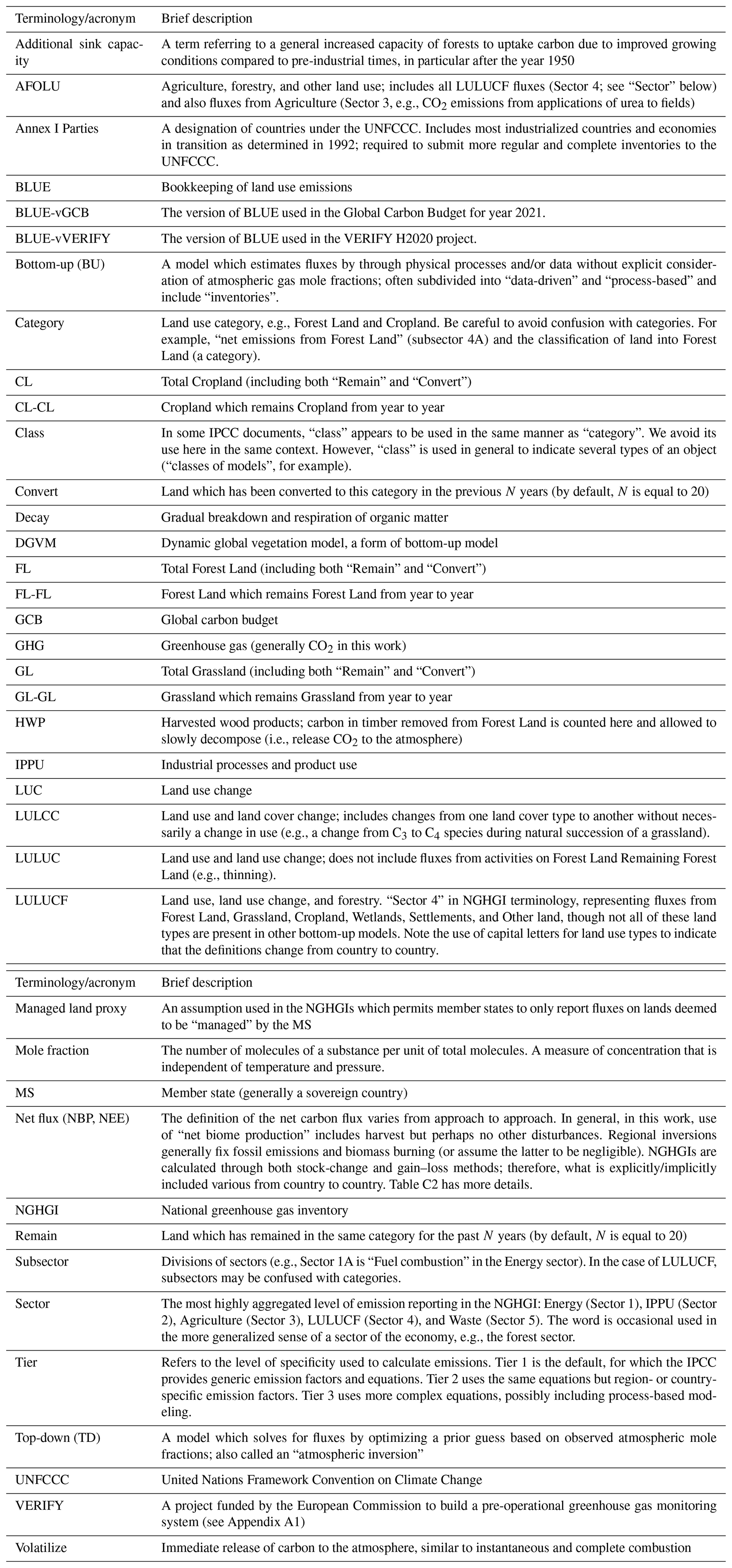
Table A2 Country grouping used for comparison purposes between BU and TD emissions as reported for the country- and regional-level synthesis plots available through the VERIFY web portal.

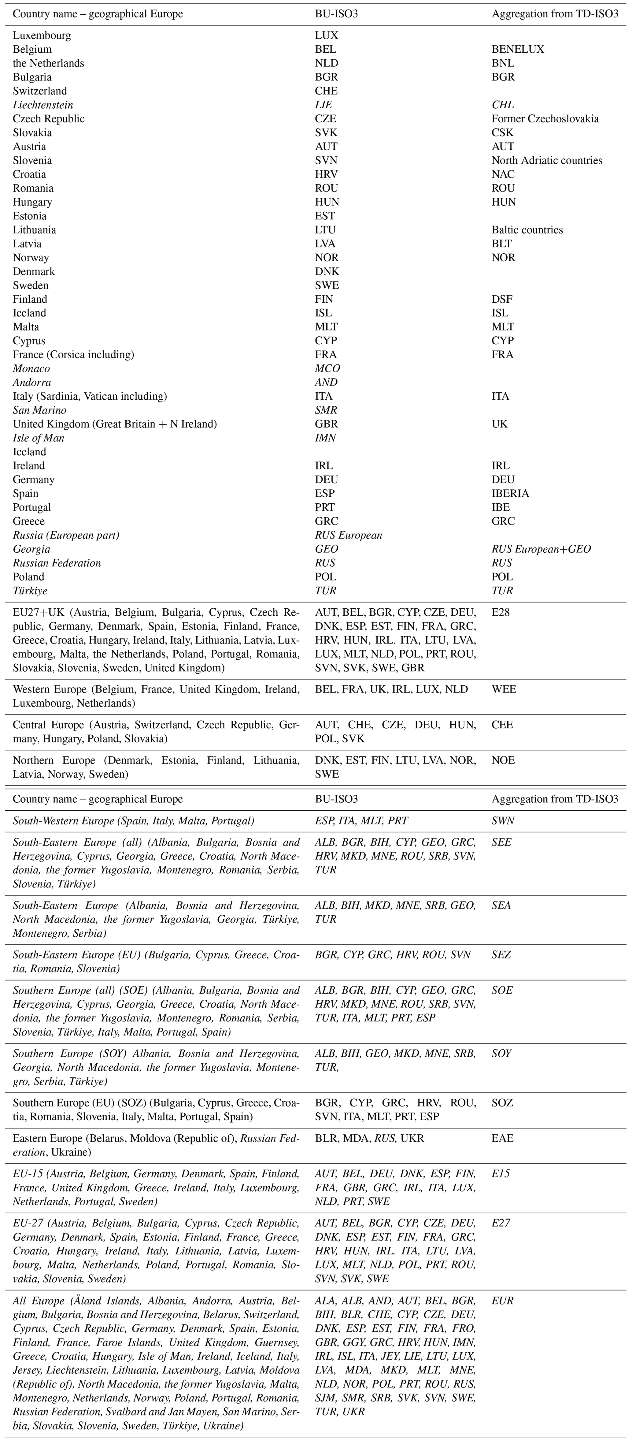
^* Countries highlighted in italics are not discussed in the current 2021 synthesis mostly because unavailability of UNFCCC NGHGI reports (non-Annex I countries are mostly developing countries). The reporting to UNFCCC is implemented through national communications (NCs) and biennial update reports (BURs): https://unfccc.int/national-reports-from-non-annex-i-parties, last access: 16 September 2023) but are present on the web portal (VERIFY Synthesis Plots, 2022).

Table A3 An overview of major changes of the current study with respect to the original (Petrescu et al., 2020) and most recent (Petrescu et al., 2021) studies of this series; n/a means a dataset was not used or available. Bold text indicates changes in this study with respect to the most recent version.

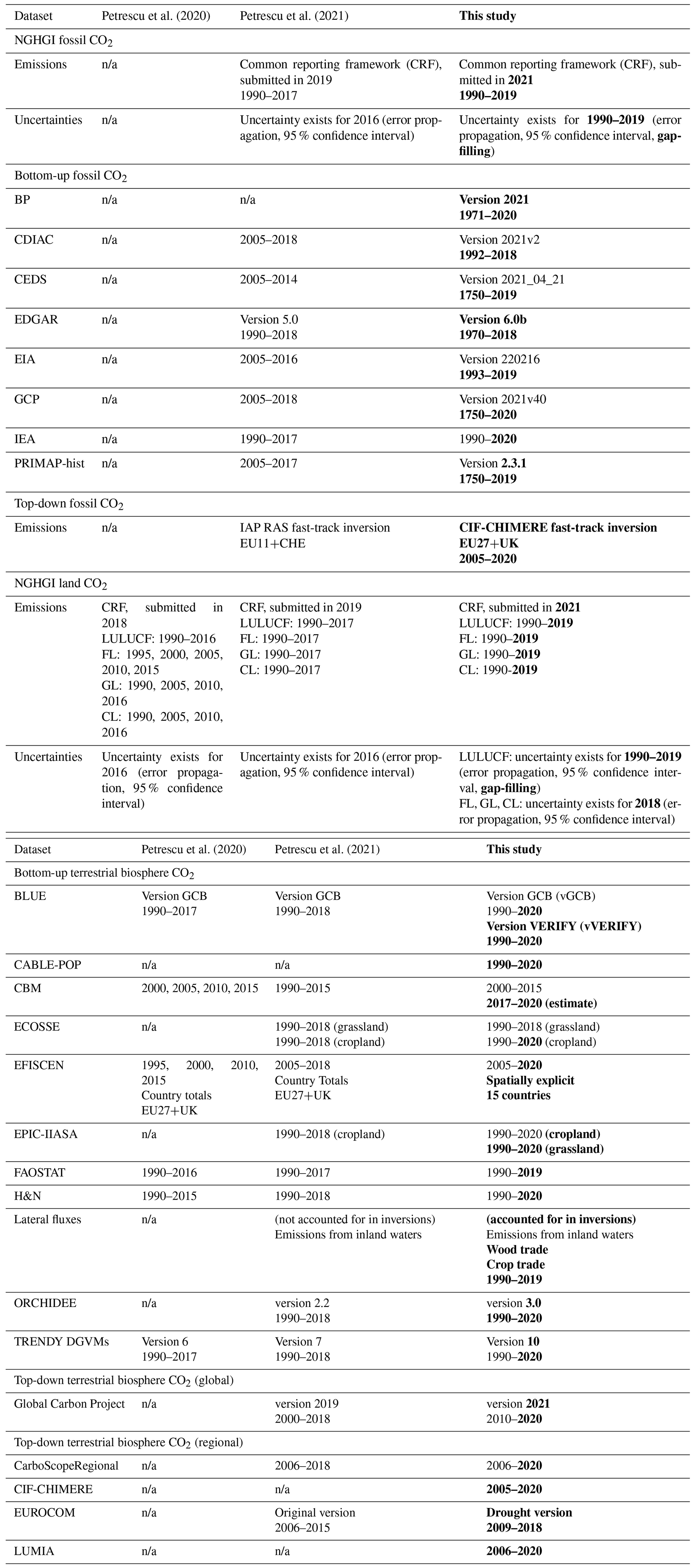
A2 UNFCCC NGHGI (2021)

Annex I NGHGIs should follow principles of transparency, accuracy, consistency, completeness, and comparability (TACCC) under the guidance of the UNFCCC (UNFCCC, 2014) and, as mentioned above, shall be completed following the 2006 IPCC guidelines (IPCC, 2006). In addition, the IPCC 2019 refinement (IPCC, 2019), which may be used to complement the 2006 IPCC guidelines, has updated sectors with additional emission sources and provides guidance on the use of atmospheric data for independent verification of GHG inventories.

Both approaches (BU and TD) provide useful insights into emissions from two different points of view. First, as outlined in Vol. 1, Chap. 6 of the 2019 IPCC refinement (IPCC, 2019), TD approaches act as an additional quality check for BU and NGHGI approaches and facilitate a deeper understanding of the processes driving changes in different elements of GHG budgets. Second, while independent BU methods do not follow prescribed standards like the IPCC guidelines, they do provide complementary information based on alternative input data at varying temporal, spatial, and sectoral resolution. This complementary information helps build trust in country GHG estimates, which form the basis of national climate mitigation policies. Additionally, BU estimates are needed as input for TD estimates. As there is no formal guideline to estimate uncertainties in TD or BU approaches, uncertainties are usually assessed from the spread of different estimates within the same approach, though some groups or institutions report uncertainties for their individual estimates using a variety of methods, for instance, by performing Monte Carlo sensitivity simulation by varying input data parameters. However, this can be logistically and computationally difficult when dealing with complex process-based models.

Despite the important insights gained from complementary BU and TD emission estimates, it should be noted that comparisons with the NGHGI are not always straightforward. BU estimates often share common methodology and input data, and through harmonization, structural differences between BU estimates and NGHGIs can be interpreted. However, the use of common input data restricts the independence between the datasets and, from a verification perspective, may limit the conclusions drawn from the comparisons. On the other hand, TD estimates are constrained by independent atmospheric observations and can serve as an additional, potentially independent, quality check for NGHGIs. Nonetheless, structural differences between NGHGIs (what sources and sinks are included, and where and when emissions/removals occur) and the actual fluxes of GHGs to the atmosphere must be taken into account during comparison of estimates. While NGHGIs go through a central QA/QC review process, the UNFCCC reporting requirements do not mandate large-scale observation-derived verification. Nevertheless, the individual countries may use atmospheric data and inverse modeling within their data quality control, quality assurance, and verification processes, with expanded and updated guidance provided in Chap. 6 of the 2019 refinement of IPCC 2006 guidelines (IPCC, 2019). So far, only a few countries (e.g., Switzerland, UK, New Zealand, and Australia) have used atmospheric observations to constrain national emissions and documented these verification activities in their national inventory reports for CH₄ and F gases (Bergamaschi et al., 2018), and none do so for CO₂.

Under the UNFCCC and its Kyoto Protocol, national GHG inventories are the most important source of information to track progress and assess climate protection measures by countries. In order to build mutual trust in the reliability of GHG emission information provided, national GHG inventories are subject to standardized reporting requirements, which have been continuously developed by the Conference of the Parties (COP).¹¹ The calculation methods for the estimation of greenhouse gasses in the respective sectors is determined by the methods provided by the 2006 IPCC Guidelines for National Greenhouse Gas Inventories (IPCC, 2006). These guidelines provide detailed methodological descriptions to estimate emissions and removals, as well as recommendations to collect the activity data needed. As a general overall requirement, the UNFCCC reporting guidelines stipulate that reporting under the convention and the Kyoto Protocol must follow the five key principles of transparency, accuracy, completeness, consistency, and comparability (TACCC).

The reporting under UNFCCC shall meet the TACCC principles. The three main GHGs are reported in time series from 1990 up to 2 years before the due date of the reporting. The reporting is strictly based on source category and is done under the common reporting format (CRF) tables, downloadable from the UNFCCC official submission portal: https://unfccc.int/ghg-inventories-annex-i-parties/2021 (last access: September 2023).

NGHGI uncertainties

The presented uncertainties in the reported emissions of the individual countries and the EU27+UK bloc were calculated by using the methods and data used to compile the official GHG emission uncertainties that are reported by the EU under the UNFCCC (2022a). The EU uncertainty analysis reported in the bloc's national inventory report (NIR) is based on country-level, approach 1 uncertainty estimates (IPCC, 2006, Vol. 1, Chap. 3) that are reported by EU member states, Iceland, and the United Kingdom under Article 7(1)(p) of EU (2013). These country-level uncertainty estimates are typically reported at the beginning of a submission cycle and are not always revised with updated CRF submissions later in the submission cycle. Furthermore, the compiled uncertainties of some countries are incomplete (e.g., uncertainties not estimated for LULUCF and/or indirect CO₂ emissions; certain subsector emissions are confidential), and the sector and gas resolution at which uncertainties are provided vary between the countries. The EU inventory team therefore implements a procedure to harmonize and gap-fill these uncertainty estimates. A processing routine reads the individual country uncertainty files that are preformatted manually to assign consistent sector and gas labels to the respective estimates of emissions/removals and uncertainties. The uncertainty values are then aggregated to a common sector resolution, at which the emissions and removals reported in the uncertainty tables of the countries are then replaced with the respective values from the final CRF tables of the countries. Due to the issue of incompleteness mentioned above, the country-level data are then screened to identify residual GHG emissions and removals for which no uncertainty estimates have been provided. Where sectors are partially complete, the residual net emission is quantified in CO₂ equivalents and incorporated. An uncertainty is then estimated, by calculating the overall sector uncertainty of the sources and sinks that were included in that country's reported uncertainty estimates and assigning this percentage average to the residual net emission. In cases where for certain sectors no uncertainties have been provided at all (e.g., indirect CO₂ emissions, LULUCF), an average (median) sector uncertainty in percent is calculated from all the countries for which complete sectoral emissions and uncertainties were reported, and this average uncertainty is assigned to the country's sector GHG total reported in its final CRF tables.

The country-level uncertainties presented in this paper, have been compiled using this same processing routine and using the uncertainties and CRF data reported by the countries in the 2021 submission. However, here the method has been expanded to gap-fill at the individual greenhouse gas level (CO₂ emissions and removals only) rather than at the aggregate GHG level. Furthermore, the expanded method here assigns the subsectoral uncertainties to the emissions and removals of the entire time series (1990–2019), rather than just the base year and latest year of the respective time series. This allows uncertainties to be sensitive to the subsectoral contributions to sectoral and national total emissions, which of course change over time. For each year of the time series, uncertainties in the total and sectoral CO₂ emissions are calculated using Gaussian error propagation, by summing the respective subsectoral uncertainties (expressed in kt CO₂) in quadrature and assuming no error correlation. In contrast, for the EU27+UK bloc, uncertainties in the total and sectoral CO₂ emissions were calculated to take into account error correlations between the respective country estimates at the subsector level. This was done by applying the same methods and assumptions described in the 2022 EU NIR (UNFCCC, 2022a). The subsector resolution applied for gap-filling allows the routine to access respective data on emission factors from CRF table “Summary 3” and apply correlation coefficients (r) when aggregating the uncertainties. For a given subsector, it is assumed that the errors of countries using default factors are completely correlated (r=1), while errors of countries using country-specific factors are assumed uncorrelated (r=0). For countries using a mix of default and country-specific factors at the given subsector level, it is assumed that these errors are partially correlated (r=0.5) with one another and with the errors of countries using the default factors only.

Based on these correlation assumptions, the routine then aggregates CO₂ emissions/removals and uncertainties for the specified subsector resolution at the EU27+UK level. Uncertainties at sector total level are then aggregated from the subsector estimates assuming no correlation between subsectors. However, for countries reporting very coarse resolution estimates (e.g., total sector CO₂ emissions/removals) or where the sector has been partially or completely gap-filled, it is assumed that these uncertainties are partially correlated (r=0.5) with one another and with the other reported subsector level estimates. Level uncertainties on the total EU27+UK CO₂ emissions and removals (with and without LULUCF) are then aggregated from the sector estimates assuming no error correlation between sectors.

Note that the above procedure does not apply to LULUCF categories (FL, CL, and GL). Estimates for these values were taken directly from the EU NIR (2021) without gap-filling or consideration of correlations. An uncertainty greater than 100 % implies that either a sink or a source is possible. As the values are given for only 1 single year, this value is applied uniformly across the whole time series.

A3 Fossil CO₂ emissions

A3.1 Bottom-up emission estimates

For further details of all datasets, see Andrew (2020).

UNFCCC NGHGI (2021)

The UNFCCC NGHGI CO₂ emissions/removals include estimates from five key sectors for the EU27+UK: 1 Energy, 2 Industrial processes and product use (IPPU), 3 Agriculture, 4 LULUCF, and 5 Waste. The tiers method that a country applies depends on the national circumstances and the individual conditions of the land, which explains the variability of uncertainties among the sector itself as well as among EU countries. This annual published dataset includes all CO₂ emission sources for those countries, as well as for most countries for the period 1990 to year t−2. Some eastern European countries' submissions began in the 1980s.

Information on uncertainty calculation in the NGHGIs is found above in the general section on the NGHGI.

EDGAR v6.0

The first edition of the Emissions Database for Global Atmospheric Research was published in 1995. The dataset now includes almost all sources of fossil CO₂ emissions, is updated annually, and reports data for 1970 to year n−1. Estimates for v6.0 are provided by sector. Emissions are estimated fully based on statistical data from 1970 till 2018 https://data.jrc.ec.europa.eu/dataset/97a67d67-c62e-4826-b873-9d972c4f670b (last access: 16 September 2023).

Uncertainties. EDGAR uses emission factors (EFs) and activity data (AD) to estimate emissions. Both EFs and AD are uncertain to some degree, and when combined, their uncertainties need to be combined too. To estimate EDGAR's uncertainties (stemming from a lack of knowledge of the true value of the EF and AD), the methodology devised by IPCC (2006, Chap. 3) is adopted (Solazzo et al., 2021), including the use of default uncertainties. The overall relative uncertainty in emissions is thus given by simple error propagation for the product of two variables, where the overall relative uncertainty is the square root of the sum of squares of the relative uncertainties of the EF and AD. A lognormal probability distribution function is assumed in order to avoid negative values, and uncertainties are reported as the 95 % confidence interval according to IPCC (2006, Chap. 3, Eq. 3.7). For emission uncertainty in the range 50 % to 230 %, a correction factor is adopted as suggested by Frey et al. (2003) and IPCC (2006, Chap. 3, Eq. 3.4). Uncertainties are published in Solazzo et al. (2021).

BP

BP releases its “Statistical Review of World Energy” annually in June, the first report being published in 1952. Primarily an energy dataset, BP also includes estimates of fossil fuel CO₂ emissions derived from its energy data (BP, 2011, 2017). The emission estimates are totals for each country starting in 1965 to year n−1.

CDIAC

The original Carbon Dioxide Information Analysis Center included a fossil CO₂ emissions dataset that was long known as CDIAC. This dataset is now produced at Appalachian State University and has been renamed CDIAC-FF (CDIAC, 2022). It includes emissions from fossil fuels (including gas flaring) and cement production from 1751 to year n−3. Fossil fuel emissions are derived from UN energy statistics, and cement emissions are from USGS production data.

EIA

The US Energy Information Administration publishes international energy statistics and from these derives estimates of CO₂ emissions from energy combustion based on energy consumption. Data are currently available for the period 1980–2016.

IEA

The International Energy Agency publishes international energy statistics and from these derives estimates of CO₂ emissions from energy combustion. In addition, the IEA also estimates emissions from the use of coal in the iron and steel industry, while not providing any other IPPU estimates. Emission estimates start in 1960 for OECD members and 1971 for non-members, and they run through to year n−1 for OECD members' totals and year n−2 for members' details and non-members. Most subsector-level data from the IEA are available for a fee, although some high-level emissions data can be accessed free of charge.

GCP

The Global Carbon Project includes estimates of fossil CO₂ emissions in its annual global carbon budget publication. These include emissions from fossil fuels and cement production for the period 1750 to year n−1. GCP's fossil CO₂ dataset was once entirely derived solely from CDIAC's dataset, with some extension using BP data, but this has since changed as described in Andrew and Peters (2022).

CEDS

The Community Emissions Data System has included estimates of fossil CO₂ emissions since 2018, with an irregular update cycle (CEDS, 2022). Energy data are directly from IEA, but emissions are scaled to higher-priority sources, including national inventories. Almost all emission sources are included, and estimates are published for the period 1750 to year n−1. Estimates are provided by subsector.

PRIMAPv2.2

The PRIMAP-hist dataset combines several published datasets to create a comprehensive set of greenhouse gas emission pathways for every country and GHG covered by the Kyoto Protocol, covering the years 1850 to 2018, and all UNFCCC (United Nations Framework Convention on Climate Change) member states as well as most non-UNFCCC territories. The data resolve the main IPCC (Intergovernmental Panel on Climate Change) 2006 categories. For CO₂, CH₄, and N₂O, subsector data for Energy, industrial processes and product use (IPPU), and Agriculture are available. Due to data availability and methodological issues, version 2.2 of the PRIMAP-hist dataset does not include emissions from land use, land use change, and forestry (LULUCF). More info is available at https://zenodo.org/record/4479172#.YUsc6p0zbIU (last access: March 2023).

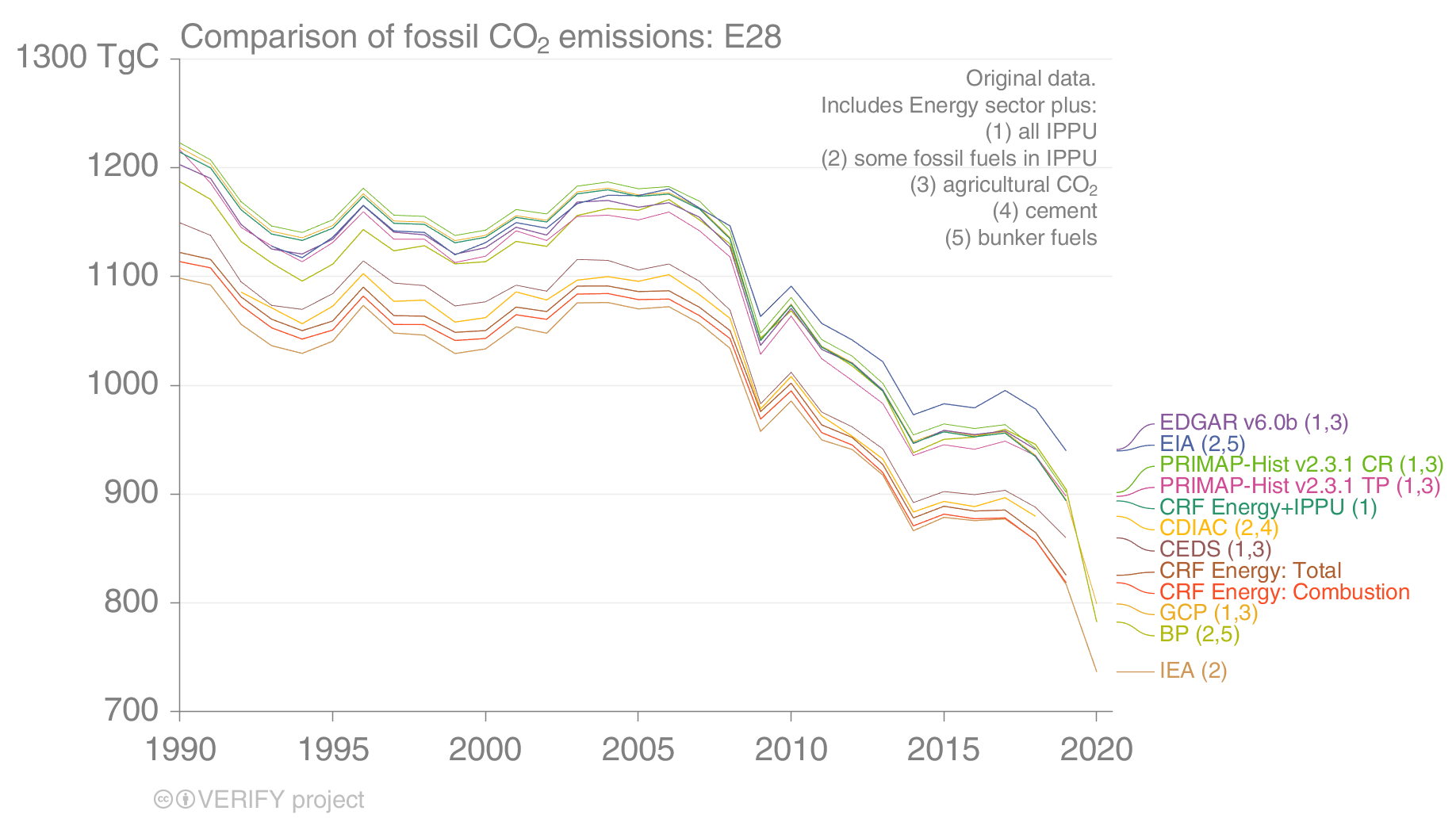
Figure A1 Comparison of EU27+UK fossil CO₂ emissions from multiple inventory datasets. Identical to Fig. 2, except that no system boundary harmonization has been done. CDIAC does not report emissions prior to 1992 for former Soviet Union countries. CRF: UNFCCC NGHGI from the common reporting format tables.

A3.2 Top-down CO₂ emission estimates

CIF-CHIMERE – fossil CO₂ emission inversion

CIF-CHIMERE is used for both CO₂ land and CO₂ fossil emission estimates, and this section only describes the CO₂ fossil estimates. The product is explained in more detail by Fortems-Cheiney and Broquet (2021).

Results from previous atmospheric inversions of the European fossil CO₂ emissions indicated that there were much larger uncertainties associated with the assimilation of CO data than with that of NO₂ data for such a purpose (Konovalov et al., 2016; Konovalov and Lvova, 2018). In this context, we have developed an atmospheric inversion configuration quantifying monthly to annual budgets of the national emissions of fossil CO₂ in Europe based on the assimilation of the long-term series of NO₂ spaceborne observations, the Community Inversion Framework (CIF), the CHIMERE regional chemical transport model (CTM), corrections to the TNO-GHGco-v3 inventory of NO_x anthropogenic emissions at 0.5^∘ horizontal resolution, and the conversion of NO_x anthropogenic emission estimates into CO₂ fossil emission estimates. For the first time, to our knowledge, variational regional inversions have been performed to estimate the European CO₂ fossil emissions using NO_x emissions from Ozone Monitoring Instrument (OMI) satellite observations. Particular attention is paid to the analysis assessing the consistency between the fossil CO₂ emission estimates from our processing chain with the fossil CO₂ emission budgets provided by the TNO-GHGco-v3 inventory based on the emissions reported by countries to UNFCCC, which are assumed to be accurate in Europe. The algorithm first optimizes NO_x emissions and then assumes a fixed ratio of NO_x to fossil CO₂ emissions. However, long-term plans include the simultaneous inversion of all three gasses (CO₂, NO₂, and CO).

The analysis is conducted over the period 2005 to 2020. CHIMERE is run over a 0.5^∘ × 0.5^∘ regular grid and 17 vertical layers, from the surface to 200 hPa, with 8 layers within the first 2 km. The domain includes 101 (longitude) × 85 (latitude) grid cells (15.25^∘ W–35.75^∘ E and 31.75–74.25^∘ N) and covers Europe. CHIMERE is driven by the European Centre for Medium-Range Weather Forecasts (ECMWF) meteorological forecast (Owens and Hewson, 2018). The chemical scheme used in CHIMERE is MELCHIOR-2, with more than 100 reactions (Lattuati, 1997; CHIMERE 2017), including 24 for inorganic chemistry. Climatological values from the LMDZ-INCA global model (Szopa et al., 2009) are used to prescribe mole fractions at the lateral and top boundaries and the initial atmospheric composition in the domain. Considering the short NO₂ lifetime, we do not consider its import from outside the domain: its boundary conditions are set to zero. Nevertheless, we take into account peroxyacetyl nitrate (PAN) for the large-scale transport of NO_x. Due to atmospheric chemistry, it represents an important NO_x reservoir, and it has a significant impact on the regional NO₂ tropospheric columns observed by OMI.

Several critical aspects of this workflow need to be highlighted: (i) Fortems-Cheiney and Broquet (2021) have not yet reported estimates of the uncertainty in the fossil CO₂ emissions (this requires the derivation of the uncertainties in the NO_x emission inversions and in the NO_x-to-FFCO₂ emission conversion) and (ii) the fossil CO₂ emission budgets provided by the TNO-GHGco-v3 inventory are based on the emissions reported by countries to UNFCCC, which are assumed to be accurate in Europe; therefore, the NO_x inversion prior estimate is consistent with the inventory estimates (with respect to the NO_x-to-FFCO₂ emission conversion used to infer fossil CO₂ emissions from the NO_x inversions).

Uncertainty. There is no uncertainty estimate currently available for this product.

A4 Land CO₂ emissions/removals

A4.1 Bottom-up CO₂ estimates

UNFCCC NGHGI 2021 – LULUCF

For the biogenic CO₂ emissions from LULUCF (Sector 4 in the terminology of the NGHGIs), methods for the estimation of CO₂ removals differ enormously among countries and land use categories. Each country uses its own country-specific method which takes into account specific national circumstances (as long as they are in accordance with the 2006 IPCC guidelines), as well as IPCC default values, which are a “compromise between the level of detail that would be needed to create the most accurate estimates for each country and the input data likely to be available or readily obtainable in most countries” (Vol. 1, Chap. 3 of IPCC, 2006). They may, therefore, result in higher uncertainties. The EU GHG inventory underlies the assumption that the individual use of national country-specific methods leads to more accurate GHG estimates than the implementation of a single EU-wide approach (UNFCCC, 2018). Key categories for the EU27 are 4.A.1 Forest Land: land use CO₂, 4.A.2. Forest Land: land use CO₂, 4.B.1 Cropland: land use CO₂, 4.B.2 Cropland: land use CO₂, 4.C.1 Grassland: land use CO₂, 4.C.2 Grassland: land use CO₂, 4.D.1 Wetlands: land use CO₂, 4.E.2 Settlements: land use CO₂, and 4.G Harvested wood products: wood product CO₂. The tiered method that a country applies depends on the national circumstances and the individual conditions of the land, which explains the variability of uncertainties among the sector itself as well as among EU countries.

Table A4 shows the mean values of all LULUCF categories for the EU27+UK NGHGI (2021). The contribution is calculated as the percentage of the sum of the absolute values of all the categories, in order to account for differing signs.

Table A4 LULUCF categories for the EU27+UK NGHGI (2021). NA – not available

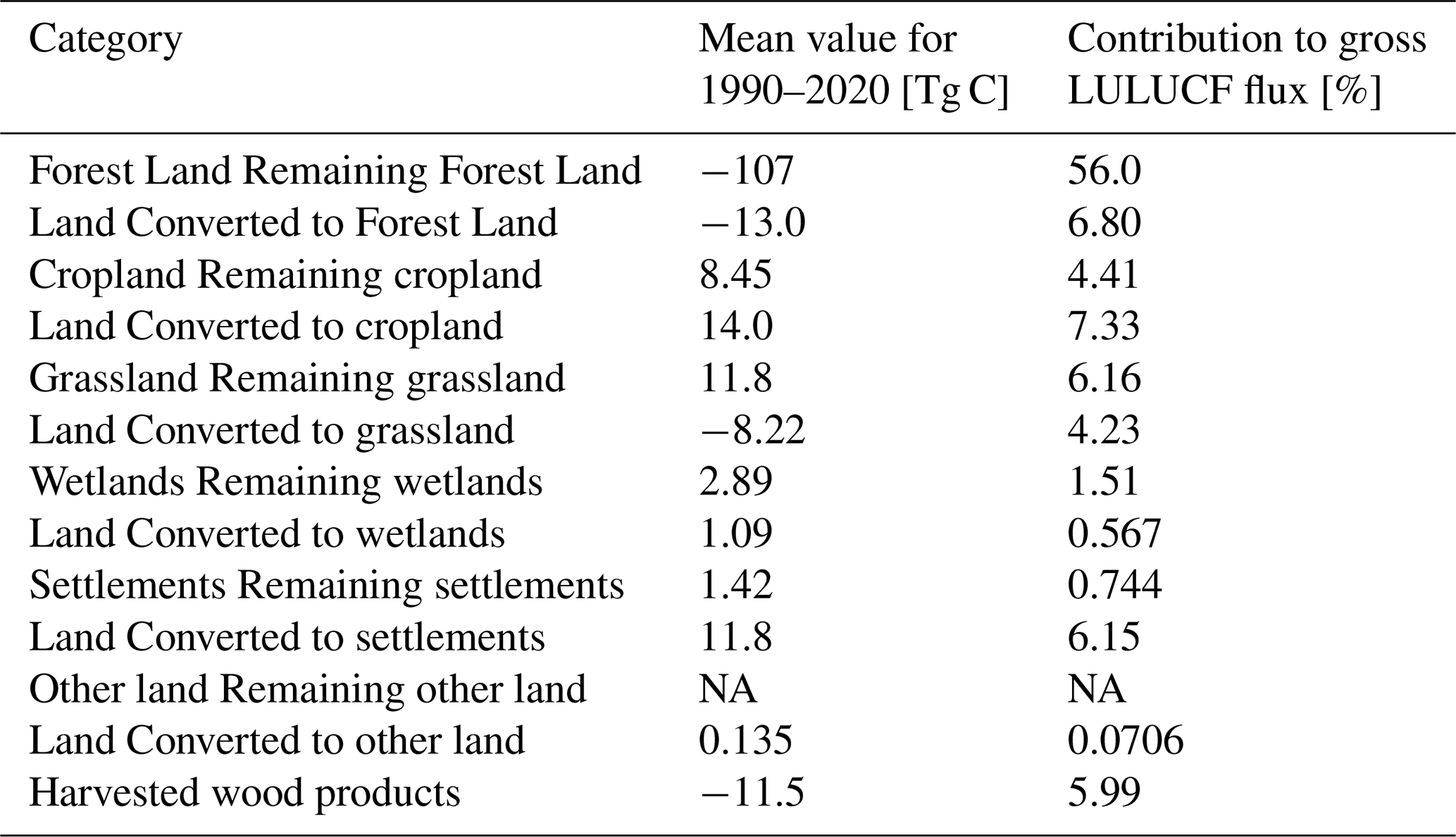
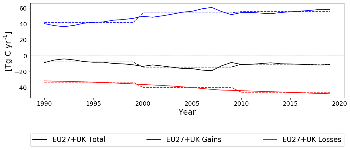
Figure A2 The gains, losses, and total HWP pools from the common reporting format tables for the European Union (convention), which covers the EU27+UK. Dashed lines show the averages for 1990–1999, 2000–2009, and 2010–2019 for easy comparison with Fig. B4.

Uncertainty. Methodology for the NGHGI UNFCCC submissions are based on Chap. 3 of 2006 IPCC Guidelines for National Greenhouse Gas Inventories and is the same as described in Appendix A2.

ORCHIDEE

ORCHIDEE is a general ecosystem model designed to be coupled to an atmospheric model in the context of modeling the entire Earth system. As such, ORCHIDEE calculates its prognostic variables (i.e., a multitude of carbon, water, and energy fluxes) from the following environmental drivers: air temperature, wind speed, solar radiation, air humidity, precipitation, and atmospheric CO₂ mole fraction. As the run progresses, vegetation grows on each pixel, divided into 15 generic types (e.g., broadleaf temperate forests, C₃ crops), which cycle carbon between the soil, land surface, and atmosphere through such processes such as photosynthesis, litter fall, and decay. Limited human activities are included through the form of generic wood and crop harvests, which remove aboveground biomass on an annual basis. The version reported here, ORCHIDEE-N v3, includes a dynamic nitrogen cycle coupled to the vegetation carbon cycle which results in, among other things, limitations on photosynthesis in nitrogen-poor environments (Vuichard et al., 2019)

Among other environmental indicators, ORCHIDEE simulates positive and negative CO₂ emissions from plant uptake; soil decomposition; and harvests across forests, grasslands, and croplands. Activity data are based on land use and land cover maps. For VERIFY, pixel land cover/land use fractions were based on a combination of the land use map LUH2v2h and the land cover project of the Climate Change Initiative (CCI) program of the European Space Agency (ESA). The latter is based on purely remotely sensed methods, while the former makes use of national harvest data from the UN Food and Agricultural Organization.

LUH2v2-ESA CCI: quoted directly from Lurton et al. (2020):

We describe here the input data and algorithms used to create the land cover maps specific for our CMIP6 [Coupled Model Intercomparison Project Phase 6] simulations using the historical/future reconstruction of land use states provided as reference datasets for CMIP6 within the land use harmonization database LUH2v2h (Hurtt et al., 2020). More details are provided on the devoted web page (https://orchidas.lsce.ipsl.fr/dev/lccci, last access: 16 September 2023) which shows further tabular, graphical and statistical data. The overall approach relies on the combination of the LUH2v2 data with present-day land cover distribution derived from satellite observations for the past decades. The main task consists in allocating the land use types from LUH2v2 in the different PFTs [plant functional types] for the historical period and the future scenarios. The terrestrial biospheric vegetation in each grid cell is defined as the PFT distribution derived from the ESA-CCI land cover product for the year 2010 to which pasture fraction and crop fraction from LUH2v2 (for the year 2010) have been subtracted from grass and crop PFTs. This characterization of the terrestrial biospheric vegetation in terms of PFT distribution is assumed invariant in time and is used for both the historical period and the different future scenarios.

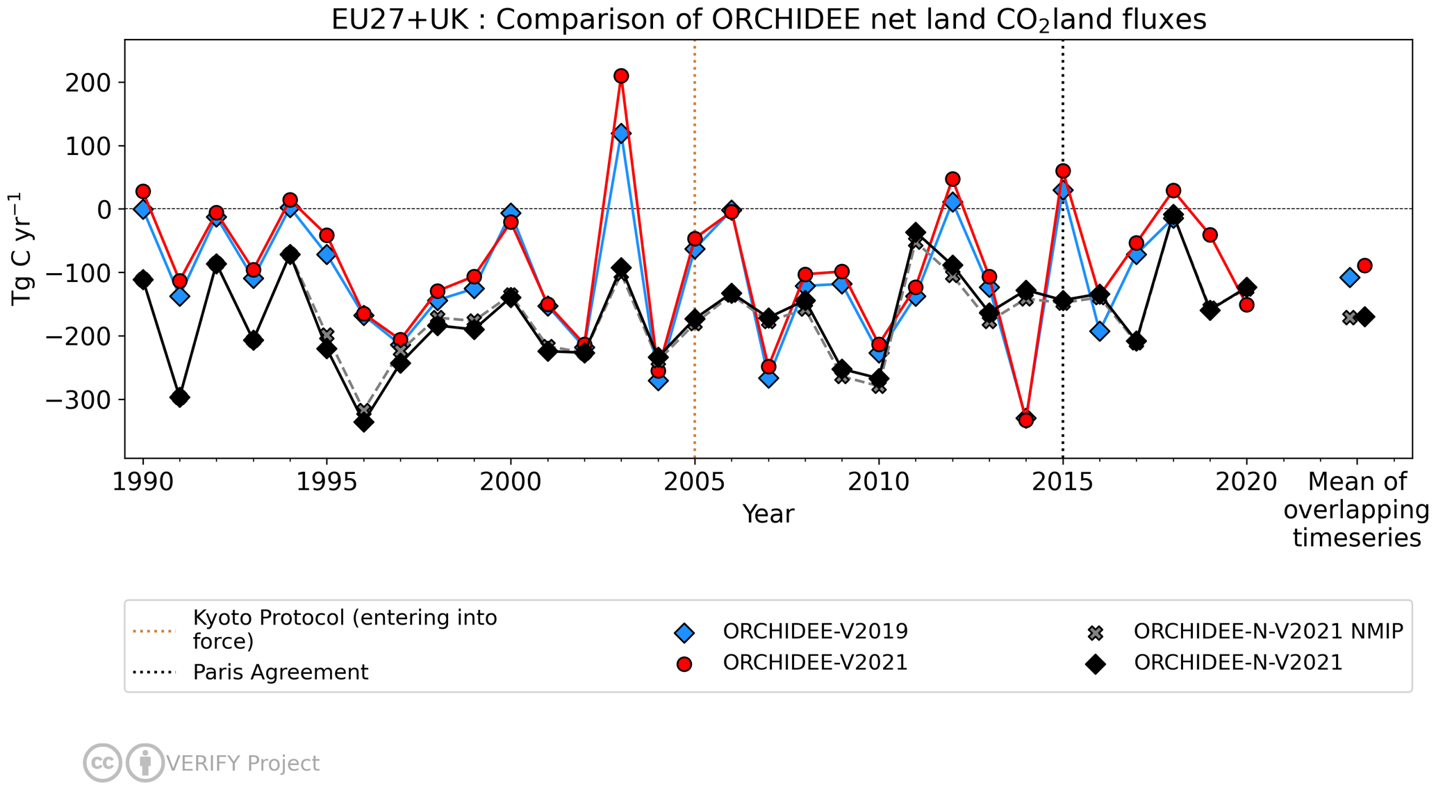
Figure A3 A comparison of the version of ORCHIDEE used in previous synthesis of Petrescu et al. (2021) compared to the same version using the forcing prepared for this work (ORCHIDEE-V2021) and the version with the coupled C–N cycle from this work (ORCHIDEE-N-V2021). For the current work, both the version shown with the Europe-specific nitrogen forcing prepared under VERIFY for the years 1995–2018 (ORCHIDEE-N-V2021) and that using the standard nitrogen forcing from the N₂O Model Intercomparison Project (NMIP; Tian et al., 2018) as supplied to the TRENDY model intercomparison are shown (ORCHIDEE-N-V2021 NMIP).

Uncertainty. In the ORCHIDEE model, uncertainty arises from three primary sources: parameters, forcing data (including spatial and temporal resolution), and model structure. Some researchers argue that the initial state of the model (i.e., the values of the various carbon and water pools at the beginning of the production run, following model spinup) represents a fourth area. However, the initial state of this version of ORCHIDEE is defined by its equilibrium state and therefore a strong function of the parameters, forcing data, and model structure, with the only independent choice being the target year of the initial state. Out of the three primary areas of uncertainty, the climate forcing data are dictated by the VERIFY project itself, thus removing that source from explaining observed differences among the models, although it can still contribute to uncertainty between the ORCHIDEE results and the national inventories. The land use/land cover maps, another major source of uncertainty for ORCHIDEE carbon fluxes, have also been harmonized to a large extent between the bottom-up carbon budget models in the project. Parameter uncertainty and model structure thus represent the two largest sources of potential disagreement between ORCHIDEE and the other bottom-up carbon budget models. Computational cost prevents a full characterization of uncertainty due to parameter selection in ORCHIDEE (and dynamic global vegetation models in general), and uncertainties in model structure require the use of multiple models of the same type but including different physical processes. Such a comparison has not been done in the context of VERIFY, although the results from the TRENDY suite of models shown in Fig. 5 give a good indication of this. Figure A3 shows a small influence from the nitrogen forcing, likely because the European nitrogen forcing is only available from 1995–2018 and ORCHIDEE carries out almost 500 years of simulation prior to this point. Many major carbon pools (i.e., woody biomass, soil carbon) have built up a large amount of inertia over that time and are unlikely to undergo dramatic changes for any realistic forcing over the past. A similar conclusion can be reached from simulations ORCHIDEE-V2019 and ORCHIDEE-V2021 in Fig. A3, which only differ in meteorological forcing from 1981–2020.

CABLE-POP

CABLE-POP (Haverd et al., 2018) is a global terrestrial biosphere model developed around a core biogeophysics module (Wang and Leuning, 1998) and a biogeochemistry module including cycles of nitrogen and phosphorus (Wang et al., 2010). Only nitrogen cycling was turned on for the present simulations. The model also includes modules simulating woody demography (Haverd et al., 2013) as well as land use change and land management (Haverd et al., 2018). The model distinguishes seven plant functional types which can co-occur in a given grid cell. CABLE-POP does not simulate (natural) dynamic vegetation, and the distribution and cover fraction of PFTs is only affected by land use change. Forest demography (establishment, age class distribution, mortality) is accounted for in the simulations, as are natural disturbances and forest management (wood harvest). For the simulations described here, a baseline land cover map was created from the HILDA+ dataset for the year 1901, and vegetation classes in the dataset were reclassified to correspond to PFTs represented in CABLE-POP. Land use transitions and land management (harvest) were prescribed from the LUH2v2h dataset over the entire simulation period. Crops and pastures are treated as C₃ grasses but are subject to agricultural harvest fluxes as given by LUH2v2h. The use of HILDA+ data for the land cover distribution and the LUH2v2h for the representation of land cover/land use change likely introduced additional uncertainties resulting from a potential mismatch between the two datasets.

CBM

The Carbon Budget Model, developed by the Canadian Forest Service (CBM-CFS3), can simulate the historical and future stand- and landscape-level C dynamics under different scenarios of harvest and natural disturbances (fires, storms), according to the standards described by the IPCC (Kurz et al., 2009). Since 2009, the CBM has been tested and validated by the Joint Research Centre of the European Commission (EC-JRC), and adapted to the European forests. It is currently applied to 26 EU member states, both at country and NUTS2 levels (Pilli et al., 2016).

Based on the model framework, each stand is described by area, age, and land use classes and up to 10 classifiers based on administrative and ecological information and on silvicultural parameters (such as forest composition and management strategy). A set of yield tables define the merchantable volume production for each species, while species-specific allometric equations convert merchantable volume production into aboveground biomass at stand level. At the end of each year, the model provides data on the net primary production (NPP), carbon stocks, and fluxes, as the annual C transfers between pools and to the forest product sector.

The model can support policy anticipation, formulation, and evaluation under the LULUCF sector, and it is used to estimate the current and future forest C dynamics, both as a verification tool (i.e., to compare the results with the estimates provided by other models) and to support the EU legislation on the LULUCF sector (Grassi et al., 2018a). In the biomass sector, the CBM can be used in combination with other models to estimate the maximum wood potential and the forest C dynamic under different assumptions of harvest and land use change (Jonsson et al., 2018).

Uncertainty. Quantifying the overall uncertainty of CBM estimates is challenging because of the complexity of each parameter. The uncertainty in CBM arises from three primary sources: parameters, forcing data (including spatial and temporal resolution), and model structure. It is linked to both activity data and emission factors (area and biomass volume implied by the species-specific equation to convert the merchantable volume to total aboveground biomass (used as a biomass expansion factor)) as well as to the capacity of each model to represent the original values – in this case estimated through the mean percentage difference between the predicted and observed values. A detailed description of the uncertainty methodology is found in Pilli et al. (2017).

Explanatory note on the extrapolation of “net biome productivity” for the period 2017–2020 (Matteo Vizzarri, Roberto Pilli, Giacomo Grassi, EC-JRC)

•  

  Background. We performed a linear extrapolation of forest net biome productivity (NBP) by country (EU25 member states and UK) in the period 2017–2020 based on the correlation between NBP and harvest from the period 2000–2015. Cyprus and Malta are excluded from the analysis because of missing historical data.

•  

  Input data. Table A5 reports a summary of input data sources.

Table A5 Main input data used in the extrapolation of NBP for the period 2017–2020.

•  

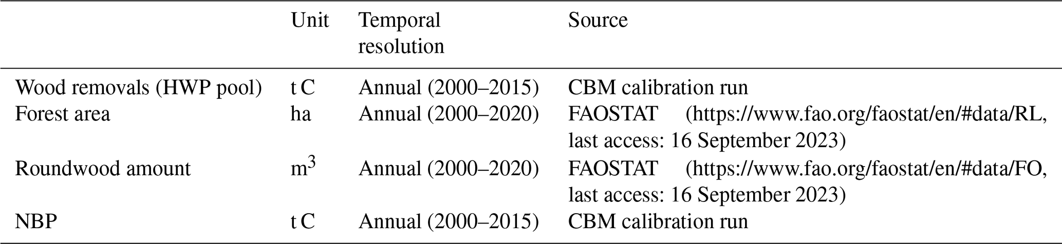
  Assessment procedure. The extrapolation of the NBP for the period 2017–2020 was obtained throughout the following steps:

1. For each country (EU25 member states + UK), we first calculated the average conversion factor – representing a correspondence between 1 t of biomass carbon removed and 1 m³ of wood per hectare – for the period 2000–2015 through Eq. (1):

   $$\begin{array}{}\text{(A1)}& {\mathrm{CF}}_{\text{2000–2015}}={\sum }_{t=\mathrm{2000}}^{\mathrm{2015}}{\displaystyle \frac{{\mathrm{HWP}}_t}{\frac{{\mathrm{RW}}_t}{A_{\mathrm{2015}}}}},\end{array}$$

   where CF_2000–2015 is the average conversion factor per hectare in the period 2000–2015 (t C m⁻³ ha⁻¹); HWP_t is the carbon content per hectare in harvested wood products in year t (t C yr⁻¹), as derived from the CBM model run; RW is the total roundwood removals in year t (m³ yr⁻¹) (source: FAOSTAT, https://www.fao.org/faostat/en/#data/FO, last access: 16 September 2023); and A₂₀₁₅ is the managed forest area in year 2015 (ha; source: Forest Europe, 2015).

2. Using the average conversion factor estimated in Eq. (1), we converted, for each country, the total roundwood removals per hectare derived from FAOSTAT for the period 2017–2020, to the corresponding amount of carbon removals per ha, through Eq. (2):

   $$\begin{array}{}\text{(A2)}& \begin{array}{rl}{\mathrm{HWP}}_{\mathrm{conv}},\text{2017–2020}& ={\mathrm{CF}}_{\text{2000–2015}}\\ & \cdot \left({\displaystyle \frac{{\mathrm{RW}}_t}{A_{\mathrm{2015}}}}\right)\end{array}\end{array}$$

   where HWP_conv is the amount of carbon removals per hectare in year t (t C ha⁻¹ yr⁻¹), CF_2000–2015 is the average conversion factor per hectare in the period 2000–2015 (t C m⁻³ ha⁻¹), RW_t is the total roundwood in year t (m³ yr⁻¹) (source: FAOSTAT, https://www.fao.org/faostat/en/#data/FO, last access: 16 September 2023), and A₂₀₁₅ is the managed forest area in the year 2015 (ha).

3. Then, for each country and the period 2000–2015, we performed a linear regression to search for significant correlation between the harvest amount (i.e., HWP in t C ha⁻¹ yr⁻¹) and NBP, according to the generalized equation:

   $$\begin{array}{}\text{(A3)}& \mathrm{NBP}=a+b\cdot \left(\mathrm{HWP}\right).\end{array}$$

   In this case, we assumed NBP as the dependent variable (t C ha⁻¹ yr⁻¹) and the amount of harvest (t C ha⁻¹ yr⁻¹) as the main driver affecting the short-term evolution of NBP, in the absence of other exogenous natural disturbances; a is the intercept of the linear trend line; b is the coefficient of the independent variable harvest amount (i.e., HWP) (m³ ha⁻¹ yr⁻¹). This approach is consistent with the methodological assumptions reported in Jonsson et al. (2021).

4. We finally calculated the NBP in the period 2017–2020 for each country through Eq. (4):

   $$\begin{array}{}\text{(A4)}& {\mathrm{NBP}}_{t,m}={\left(a+b\cdot {\mathrm{HWP}}_{\mathrm{conv}}\right)}_{t,m},\end{array}$$

   where NBP_t,m is the net biome productivity for year t and country m (t C ha⁻¹ yr⁻¹), a_t,m is the intercept of the linear trend line for year t and country m, b_t,m is the coefficient of the independent variable in the trend line, and HWP_conv (t,m) is the amount of carbon removal per hectare for year t and country m (t C ha⁻¹ yr⁻¹).

Forest area and parameters used in Eq. (4) by country are reported in Table A6.

Table A6 Country-based forest area in 2015 and parameters used in Eq. (4). ^* significant (p<0.05); ns: not significant (p>0.05).

•  

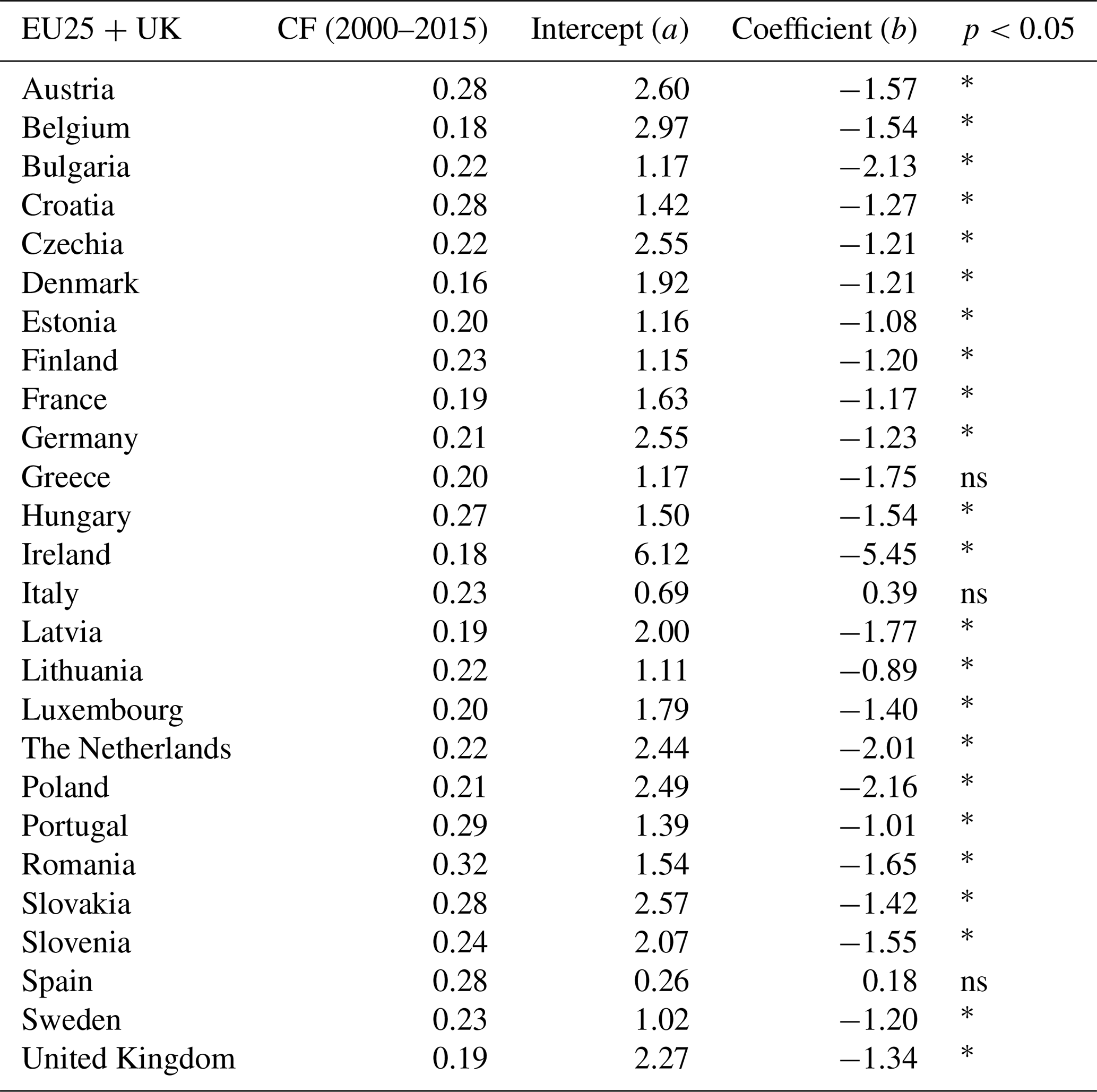
  Additional notes. Because of biased estimates, values for the year 2016 were excluded from this analysis.

  Extrapolated NBP for the Czech Republic, Ireland, and the Netherlands were negative (thus showing emissions) because of an increase in harvest in the corresponding years (2017–2020) compared to the previous period 2000–2015. Estonia shows negative extrapolated NBP only for the year 2018.

EFISCEN-Space

The European Forest Information SCENario Model (EFISCEN) is a large-scale forest model that projects forest resource development on a regional to European scale. The model uses aggregated national forest inventory data as a main source of input to describe the current structure and composition of European forest resources. The model projects the development of forest resources, based on scenarios for policy, management strategies, and climate change impacts. With the help of biomass expansion factors, stem wood volume is converted into whole-tree biomass and subsequently to whole-tree carbon stocks. Information on litter fall rates, felling residues, and natural mortality is used as input into the soil module YASSO (Liski et al., 2005), which is dynamically linked to EFISCEN and delivers information on forest soil carbon stocks. The core of EFISCEN was developed by Ola Sallnäs at the Swedish Agricultural University (Sallnäs, 1990). It has been applied to European countries in many studies since then, dealing with a diversity of forest resource and policy aspects. A detailed model description is given by Verkerk et al. (2016), with online information on availability and documentation of EFISCEN at http://efiscen.efi.int (last access: 16 September 2023). The model and its source code are freely available, distributed under the GNU General Public License conditions (http://www.gnu.org/licenses/gpl-3.0.html, last access: 16 September 2023).

In this report the follow-up of the EFISCEN was used, called EFISCEN-Space. EFISCEN-Space simulates the development of the forest at the level of the plots as measured in the national forest inventories, thereby providing a much higher spatial detail. The simulation is based on the distribution of trees over diameter classes rather than age as in the old EFISCEN. This allows for the simulation of a wider variety of stand structures, species mixtures, and management options. Similar to the EFISCEN, biomass expansion factors and the YASSO soil carbon model are used to provide carbon balances for the forest. For use within VERIFY, individual plot results are aggregated to a 0.125^∘ grid. For the moment, only 15 European member states are included, partly due to the lack of an appropriate national forest inventory in the other member states or because the data could not be shared. No formal sensitivity and uncertainty analysis has been conducted yet.

Figure 3 shows results which vary from year to year. In practice, the model was initialized with starting years depending on the country, assuming that all data applied to this year. The model then produced stock and flux changes for the subsequent 5-year period, reporting a single mean value per pixel. To compute time series for the EU27+UK, it was further assumed that these values were valid across 2005–2020. As the fluxes were given per square meter of forest, they were scaled by the total area of the forest in each pixel found on the land use/land cover maps used by the ORCHIDEE DGVM. This explains why the numbers vary from year to year; the flux per square meter of forest does not change, but the total amount of forest area changes slightly. It should be noted that country-level values available on the VERIFY website are only available for the 5-year period for which the model produces a mean result.

Uncertainties. A sensitivity analysis of EFISCEN v3 is described in detail in Chap. 6 of the user manual (Schelhaas et al., 2007). Total sensitivity is caused by especially young forest growth, width of volume classes, age of felling, and a few other variables. Scenario uncertainty comes on top of this when projecting in future. Within VERIFY, a full uncertainty analysis has been completed, enabling the estimation of uncertainty ranges of the various output variables (Schelhaas et al., 2022).

EPIC-IIASA

The Environmental Policy Integrated Climate (EPIC) model is a field-scale process-based model (Izaurralde et al., 2006; Williams, 1990) which calculates, with a daily time step, crop growth and yield; hydrological, nutrient, and carbon cycling; soil temperature and moisture; soil erosion; tillage; and plant environment control. Potential crop biomass is calculated from photosynthetically active radiation using the radiation-use-efficiency concept modified for vapor pressure deficit and the atmospheric CO₂ mole fraction effect. Potential biomass is adjusted to actual biomass through daily stress caused by extreme temperatures, water and nutrient deficiency, or inadequate aeration. The coupled organic C and N module in EPIC (Izaurralde et al., 2006) distributes organic C and N between three pools of soil organic matter (active, slow, and passive) and two litter compartments (metabolic and structural). EPIC calculates potential transformations of the five compartments as regulated by soil moisture, temperature, oxygen, tillage, and lignin content. Daily potential transformations are adjusted to actual transformations when the combined N demand in all receiving compartments exceeds the N supply from the soil. The transformed components are partitioned into CO₂ (heterotrophic respiration), dissolved C in leaching (DOC), and the receiving SOC pools. EPIC also calculates SOC loss with erosion.

The EPIC-IIASA (version EU) modeling platform was built by coupling the field-scale EPIC version 0810 with large-scale data on land cover (cropland and grasslands), soils, topography, field size, crop management practices, and grassland cutting intensity aggregated at a 1×1 km grid covering European countries (Balkovič et al., 2018, 2013). In VERIFY, a total of 10 major European crops including winter wheat, winter rye, spring barley, grain maize, winter rapeseed, sunflower, sugar beet, potatoes, soybean, and rice were used to represent agricultural production systems in European cropland. Crop fertilization and irrigation were estimated for NUTS2 statistical regions between 1995 and 2010 (Balkovič et al., 2013). For VERIFY, the simulations were carried out assuming conventional tillage, consisting of two cultivation operations and moldboard plowing prior to sowing and offset disking after harvesting of cereals. Two row cultivations during the growing season were simulated for maize and one ridging operation for potatoes. It was assumed that 20 % of crop residues are removed in the case of cereals (excluding maize), while no residues are harvested for other crops.

A total of five managed grassland types with distinct temperature requirements, biomass productivity, and phenology were used to represent the C cycle in European grasslands. High-productive generic winter pasture and tall fescue-based grasslands were used for Atlantic Europe, low fescue grasslands for the cool climates of Nordic regions and high mountains, high-productive tall fescue-based grasslands and low-productive bluegrass types for continental Europe, and low-productive bromegrass and high-productive winter pastures in the Mediterranean regions. Annual nitrogen and carbon inputs (including inorganic and manure fertilization and atmospheric N deposition) were obtained from ISIMIP3 (Jägermeyr et al., 2021). In this dataset, the annual manure production and the fraction of manure from livestock applied to cropland and rangeland were used from Zhang et al. (2017). The original manure data were regridded to 0.5^∘ spatial resolution in ISMIP3. In the model, manure is applied as an organic fertilizer with a C:N ratio of 14.5:1. The organic carbon and nitrogen are added to the fresh organic litter pool where they decompose in a manner identical to the fresh litter from vegetation, while mineral N from manure is added to the soil nitrate and ammonium pools. The distribution of herbage biomass export intensity was constructed based on Chang et al. (2016).

Uncertainty. In EPIC, uncertainties arise from three primary sources which were described in detail by ORCHIDEE. A detailed sensitivity and uncertainty analysis of EPIC-IIASA regional carbon modeling is presented in Balkovič et al. (2020).

ECOSSE (grasslands)

ECOSSE is a biogeochemical model that is based on the carbon model RothC (Jenkinson and Rayner, 1977; Jenkinson et al., 1987; Coleman and Jenkinson, 1996) and the nitrogen-model SUNDIAL (Bradbury et al., 1993; Smith et al., 1996). All major processes of the carbon and nitrogen dynamics are considered (Smith et al., 2010a, b). Additionally, in ECOSSE processes of minor relevance for mineral arable soils are implemented as well (e.g., methane emissions) to have a better representation of processes that are relevant for other soils (e.g., organic soils). ECOSSE can run in different modes and for different time steps. The two main modes are site-specific and limited data. In the later version, basic assumptions/estimates for parameters can be provided by the model. This increases the uncertainty but makes ECOSSE a universal tool that can be applied for large-scale simulations even if the data availability is limited. To increase the accuracy in the site-specific version of the model, detailed information about soil properties, plant input, nutrient application, and management can be added as available.

During the decomposition process, material is exchanged between the SOM pools according to first-order rate equations, characterized by a specific rate constant for each pool, and modified according to rate modifiers dependent on the temperature, moisture, crop cover, and pH of the soil. The model includes five pools with one of them being inert. The N content of the soil follows the decomposition of the SOM, with a stable C:N ratio defined for each pool at a given pH, and N being either mineralized or immobilized to maintain that ratio. Nitrogen released from decomposing SOM as ammonium (NH${}_{\mathrm{4}}^{+}$) or added to the soil may be nitrified to nitrate (NO${}_{\mathrm{3}}^{-}$).

For spatial simulations, the model is implemented in a spatial model platform. This allows users to aggregate the input parameter for the desired resolution. ECOSSE is a one-dimensional model, and the model platform provides the input data in a spatial distribution and aggregates the model outputs for further analysis. While climate data are interpolated, soil data are represented by the dominant soil type or by the proportional representation of the different soil types in the spatial simulation unit (this is in VERIFY a grid cell).

Uncertainty. In ECOSSE, uncertainty arises from three primary sources: parameters, forcing data (including spatial and temporal resolution), and model structure. These uncertainties are not yet quantified.

Bookkeeping models

We make use of data from two bookkeeping models: BLUE (Hansis et al., 2015) and H&N (Houghton and Nassikas, 2017).

The BLUE model provides a data-driven estimate of the net land use change fluxes. BLUE stands for “bookkeeping of land use emissions”. Bookkeeping models (Hansis et al., 2015; Houghton et al., 1983) calculate land use change CO₂ emissions (sources and sinks) for transitions between various natural vegetation types and agricultural lands. The bookkeeping approaches keep track of the carbon stored in vegetation, soils, and products before and after the land use change. In BLUE, land use forcing is taken from the Land Use Harmonization, LUH2, for estimates within the annual global carbon budget. The model provides data at annual time steps and 0.25^∘ resolution. Temporal evolution of carbon gain or loss, i.e., how fast carbon pools respire or regrow following a land use change, is based on response curves derived from literature. The response curves describe gradual respiration of vegetation and soil carbon, including transfer to product pools of different lifetimes, as well as carbon uptake due to regrowth of vegetation and subsequent refilling of soil carbon pools. In this report we present two versions of BLUE: BLUE-vVERIFY and BLUE-vGCB. The BLUEvVERIFY version is a set of runs made for VERIFY, using the Hilda+ (https://landchangestories.org/hildaplus/, last access: 16 September 2023) product (Ganzenmüller et al., 2022).

The H&N model (Houghton et al., 1983) calculates land use change CO₂ emissions and uptake fluxes for transitions between various natural vegetation types and agricultural lands (croplands and pastures). The original bookkeeping approach of Houghton (2003) keeps track of the carbon stored in vegetation and soils before and after the land use change. Carbon gain or loss is based on response curves derived from literature. The response curves describe gradual respiration of vegetation and soil carbon, including transfer to product pools of different life-times, as well as carbon uptake due to regrowth of vegetation and consequent refilling of soil carbon pools. Natural vegetation can generally be distinguished into primary and secondary land. For forests, a primary forest that is cleared can never return back to its original carbon density. Instead, long-term degradation of primary forest is assumed and represented by lowered standing vegetation and soil carbon stocks in the secondary forests. Apart from land use transitions between different types of vegetation cover, forest management practices in the form of wood harvest volumes are included. Different from dynamic global vegetation models, bookkeeping models ignore changes in environmental conditions (climate, atmospheric CO₂, nitrogen deposition, and other environmental factors). Carbon densities at a given point in time are only influenced by the land use history but not by the preceding changes in the environmental state. Carbon densities are taken from observations in the literature and thus reflect environmental conditions of the last decades. In this study an updated H&N version submitted to the GCP2021 is used.

Uncertainty. Uncertainties can be captured through simulations varying uncertain parameters, input data, or process representation. A large contribution of uncertainty can be expected from various input datasets. Apparent uncertainties arise from the land use forcing data (Gasser et al., 2020; Hartung et al., 2021; Ganzenmüller et al., 2022), the equilibrium carbon densities of soil and vegetation as well as allocation of material upon a land use transition (Bastos et al., 2021), and the response curves built to reflect carbon pool decay and regrowth after land use transitions. Furthermore, studies have shown that different accounting schemes (Hansis et al., 2015) and initialization settings at the start of the simulations (Hartung et al., 2021) lead to different emission estimates even decades later.

FAOSTAT

FAOSTAT: the Statistics Division of the Food and Agricultural Organization of the United Nations provides updates for the LULUCF CO₂ emissions for the period 1990–2019, available at https://www.fao.org/faostat/en/#data/GT (last access: June 2021), and its subdomains. The FAOSTAT emissions land use database is computed following a Tier 1 approach of IPCC (2006). Geospatial data are the source of AD for the estimates of emissions from cultivation of organic soils, biomass, and peat fires. GHG emissions are provided by countries, regions, and special groups, with global coverage, relative to the period 1990–present (with annual updates). Land use Total contains all GHG emissions and removals produced in the different land use subdomains, representing four IPCC land use categories, of which three are land use categories: forest land, cropland, grassland, and biomass burning. LULUCF emissions consist of CO₂ associated with land use and change, including management activities. CO₂ emissions/removals are computed at Tier 3 using carbon stock change. To this end, FAOSTAT uses Forest area and carbon stock data from FRA (2015), gap-filled and interpolated to generate annual time series. As a result, CO₂ emissions/removals are computed for forest land and net forest conversion, representing, respectively, IPCC categories “Forest Land” and “Forest Land converted to other land uses”. CO₂ emissions are provided as by country, regions, and special groups, with global coverage, relative to the period 1990 to the most recent available year (with annual updates), expressed as net emissions/removals as Gg CO₂, by the underlying land use emission subdomain and by aggregate (land use total).

Uncertainty. FAOSTAT uncertainties are not available.

TRENDY DGVMs

The TRENDY (trends in net land–atmosphere carbon exchange over the period 1980–2010) project represents a consortium of dynamic global vegetation models (DGVMs) following identical simulation protocols to investigate spatial trends in carbon fluxes across the globe over the past century. As DGVMs, the models require climate, carbon dioxide, and land use change input data to produce results. In TRENDY, all three of these are harmonized to make the results across the whole suite of models more comparable. In the case of VERIFY, 15 of the 16 models for TRENDY v10 (except for ISAM, which after visual inspection showed several outlier years) were used. While describing the details of all the models used here is clearly not possible, DGVMs calculate prognostic variables (i.e., a multitude of carbon, water, and energy fluxes) from the following environmental drivers: air temperature, wind speed, solar radiation, air humidity, precipitation, and atmospheric CO₂ mole fraction. As the run progresses, vegetation grows on each pixel, divided into generic types which depend on the model (e.g., broadleaf temperate forests, C₃ crops), which cycle carbon between the soil, land surface, and atmosphere, through such processes such as photosynthesis, litter fall, and decay. Limited human activities are included depending on the model, typically removing aboveground biomass on an annual basis.

Among other environmental indicators, DGVMs simulate positive and negative CO₂ emissions from plant uptake; soil decomposition; and harvests across forests, grasslands, and croplands. Activity data are based on land use and land cover maps and generally follows approach 1 as described by the IPCC 2006 guidelines (enabling calculation of only net changes from year to year). For TRENDY, pixel land cover/land use fractions were based on the land use map LUH2 (Hurtt et al., 2020) and the HYDE land use change dataset (Klein Goldewijk et al., 2017a, b). Both of these maps rely on FAO statistics on agricultural land area and national harvest data.

Uncertainty. In TRENDY v10 uncertainties are model specific and described by Friedlingstein et al. (2022). The spread of the 15 TRENDY models used by this study (Fig. 5) gives an idea of the uncertainty due to model structure in dynamic global vegetation models, as the forcing data were harmonized for all models.

Net emissions from lateral transport of carbon (crops, wood, and inland waters)

Net carbon flux due to lateral transport includes both carbon imported into a country/pixel and respired and carbon assimilated in a country/pixel and then transported to a different country/pixel before respiration.

Production and consumption of carbon do not always occur on the same grid points. This is particularly relevant for the land surface in the case of crops, wood products, and carbon transfers through the inland water network. The purpose of the work here is primarily to convert the flux changes of the top-down inversions into NGHGI-like stock changes. To convert the flux changes of the inversions (where a positive number represents a flux to the atmosphere, i.e., a source) into NGHGI-like stock changes, one needs to add the crop sink and remove the crop source. The crop sink comes from production numbers in the FAO food balance sheets, while the source is estimated by production plus import minus export (all from the FAO food balance sheets), and both terms make use of conversion factors for each commodity. We take the forestry balance sheets of FAO (production, import, and export per commodity) and convert to C mass. For a given year, the fraction of this mass that is released later in the atmosphere in each country is modeled with an e-folding decrease driven by experimental data per country (Mason Earles et al., 2012). Lateral transfers of carbon through inland waters also need to be removed from the inversion results as the terrestrial biospheric CO₂ uptake leached into the inland water network represents a carbon sink, while the fraction that is subsequently reemitted as CO₂ before reaching the ocean is a carbon source. The inland water CO₂ outgassing originates from carbon imported with runoff as dissolved CO₂ or produced in situ from the decomposition of terrestrial carbon inputs. Note further that a fraction of the net uptake of atmospheric CO₂ over the continents does not accumulate on land but is instead exported through the inland water network to the oceans; this fraction is included in the calculation. For regional carbon budgets, any river carbon export outside the boundaries of the region of interest (in this case, EU27+UK) needs to be known to separate net uptake of atmospheric C from the actual land C sink.

Carbon fluxes to the atmosphere from rivers and lakes were obtained from maps described in Zscheischler et al. (2017). These methods are similar to those described previously in Petrescu et al. (2021). The primary difference is that the updated estimates include smaller lakes and reservoirs not represented in the Global Lakes and Wetland Database through the use of a scaling law, in addition to the older results being created specifically for Europe, while the newer results are part of a global product. The emissions from the previous work totaled 25.5 Tg C yr⁻¹ for the EU27+UK, while those used here are 19.8 Tg C yr-1 (with no variability from year to year). This difference is therefore small compared to the river C export, which is included this year for the first time and averages −73.8 Tg for the period 1990–2020.

One important difference between the fluvial carbon exports reported here and those from a previous work (Ciais et al., 2021) are that those reported here are rescaled to reasonable global flux reflecting bias in inter-hemispheric exchange. Similar to Bastos et al. (2020b), the dissolved organic carbon (DOC) and particulate organic carbon (POC) exports were rescaled per basin to match the estimates of Resplandy et al. (2018). The global total organic C was finally rescaled to 500 Tg C yr⁻¹, which is considered a reasonable global number based on different reviews and synthesis efforts (Regnier et al., 2013).

A4.2 Top-down CO₂ emission estimates

For the regional inversions, atmospheric observations of CO₂ were taken from multiple sources. For CarboScopeRegional, atmospheric observations were taken from the ICOS 2021.1 ATC (ICOS RI, 2021) and the GlobalViewPlus 6.1 product (Schuldt et al., 2021a). For the CIF-CHIMERE inversions, atmospheric observations of CO₂ for the period 2005–2020 were taken from the ICOS 2021.1 ATC (ICOS RI, 2021) and SNO_SIFA L2 (SNO-IFA, 2023) releases, along with data distributed through the GlobalViewPlus 6.1 product (Schuldt et al., 2021a). For LUMIA inversions, atmospheric observations of CO₂ for the period 2006–2018 were taken from the dataset prepared for the 2018 Drought Task Force initiative (Thompson et al., 2020). For the more recent years, data were used from the ICOS 2021.1 ATC release (ICOS RI, 2021), along with data distributed through the GlobalViewPlus 7.0 product (Schuldt et al., 2021b) and, for four sites, data distributed through the World Data Center for Greenhouse Gases.

CarboScopeRegional

CarboScopeRegional (CSR) (Munassar et al., 2022): CSR is a Bayesian framework inversion system that employs a priori knowledge of the surface-atmosphere carbon fluxes to regularize the solution of the ill-posed inverse problem arising from the sparseness of observations sampled over limited geographical locations throughout the domain of interest. Due to the heterogeneity of biogenic fluxes, the convention in CSR is to optimize net ecosystem exchange (NEE) against measurements of CO₂ dry model fraction at 3-hourly temporal and 0.5^∘ horizontal resolutions, while ocean fluxes and anthropogenic emissions are prescribed given their better knowledge available compared with NEE. The prior flux uncertainty is assumed to have a uniform shape in space and time, and its spatial correlation is fitted to a hyperbolic decay function following the assumption of Kountouris et al. (2018a, b). Model–data mismatch uncertainty is defined weekly in the measurement covariance matrix varying over sites from 0.5 to 4 (ppm) according to the ability for atmospheric transport models to sample the true mole fraction at such locations (Rödenbeck, 2005). This uncertainty implicitly encompasses the combinations of atmospheric transport, representation, and measurement errors and is assumed to be independent at different locations. To separate the lateral influences originating from outside of the regional domain, the two-step scheme inversion (Rödenbeck et al., 2009) is applied to run a global inversion with the Eulerian model TM3 at coarse resolutions to provide the lateral boundary conditions to the regional inversion. In the regional inversion runs, the Lagrangian model STILT (Lin et al., 2003), forced by IFS data from ECMWF, is used to calculate the surface sensitivities “footprints” over the regional site network (receptors) at hourly temporal and 0.25^∘ spatial resolutions. Typically, the prior fluxes of CO₂ are obtained from bottom-up model estimations. Thus, the diagnostic biosphere model VPRM (Vegetation Photosynthesis and Respiration Model; Mahadevan et al., 2008) calculates the biogenic fluxes at hourly temporal resolution preserving the diurnal cycle. Ocean fluxes are obtained from the CarboScope ocean-based fluxes developed in-house by Rödenbeck et al. (2014). Emissions of fossil fuel are taken from EDGAR_v4.3 inventories updated every year based on the British Petroleum statistics (BP), and are distributed in space and time using the COFFEE approach (Steinbach et al., 2011) according to fuel type and sector.

The v2021 CSR inversions underwent updates in comparison with the previous v2019.

• v2019 from Petrescu et al. (2021) excluded observations from two sites: La Muela (LMU) in Spain, because of inconsistent datasets between releases, and Finokalia (FKL) in Greece, due to errors in the dataset. These exclusions resulted in a larger C sink from 2013 onwards (Fig. 5, lower plot). FKL observations start at this time and are the dominant impact over southeast Europe, as it is the only site located there. In v2021 inversions, we included corrected datasets from the FKL site.

• Two new flask sites were included in the v2021 inversions: Shetland Islands in the UK and Centro de Investigacion de la Baja in Spain. These sites are also used in the CarboScope global inversion that provides the far-field contributions to the EU domain.

Uncertainty. Uncertainties from top-down (TD) estimates can be reported as posterior Bayesian uncertainties. Following the methodology of Chevallier et al. (2007), the CSR inversion system computed maps of uncertainty reductions for 2006 and 2018 (Fig. A4). The reduction is carried out through an ensemble of 40 members of inversions using error realizations following a Monte Carlo (MC) approach. Circles on maps refer to locations of stations. In the inversion system, a MC method is used to generate N ensembles of realizations of prior errors and model–data mismatch errors. The inversion is repeated for each ensemble member starting from each set of prior and model–data mismatch errors to generate posterior fluxes. The posterior uncertainty is calculated as the spread over the optimized fluxes across the whole ensemble. The uncertainty reduction is then calculated as $\mathrm{1}-({\mathit{\sigma }}_{\text{post}}/{\mathit{\sigma }}_{\text{prior}})$. It is clear that larger ensembles will lead to better convergence of the error reduction. However, due to computational limitations, 40 ensemble members were selected as a good compromise.

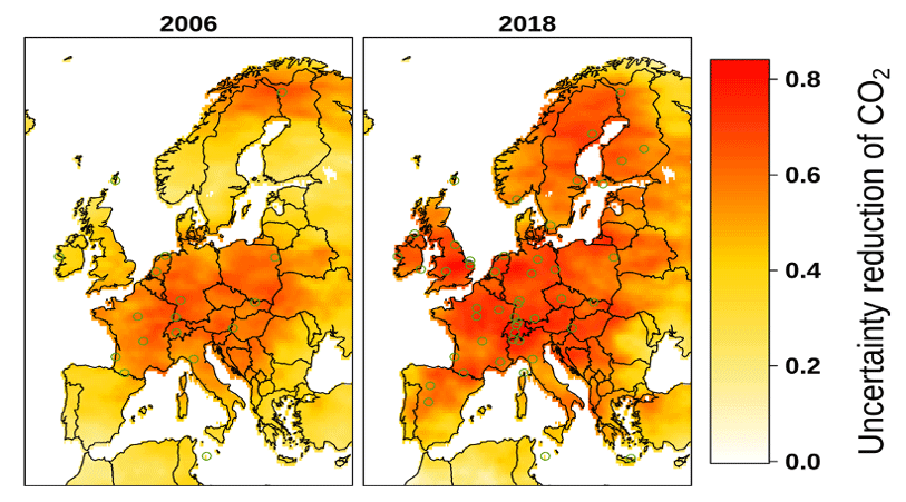
Figure A4 CSR uncertainty reduction maps computed as $\mathrm{1}-({\mathit{\sigma }}_{\mathrm{post}}/{\mathit{\sigma }}_{\mathrm{prior}})$ for 2006 and 2018 using a Monte Carlo approach focused on prior errors. The circles represent network the observation stations.

Figure A4 represents a preliminary attempt at how the inclusion of additional observation stations (additional circles in the right-side figure for Germany, Switzerland, and Finland compared to the left-side figure) might reduce the uncertainty. However, the two different simulation years (2006 and 2018) might also differ in terms of other factors which may lead to lower uncertainties in a given year (e.g., climatological conditions, such as the 2018 drought year).

Several caveats remain. When comparing the uncertainty over pixels or subregions in the domain of interest, the maps of uncertainty reduction should be interpreted together with the maps of posterior uncertainty to give a better illustration of the magnitude of uncertainty. The maps of uncertainty reduction reflect only the random uncertainties. The systematic uncertainties are still poorly characterized, including uncertainties due to atmospheric transport modeling, dependence on the prior fluxes, and the weighting between the prior and observation uncertainties. To improve knowledge of the systematic uncertainties, dedicated studies with controlled comparisons between inversions using different atmospheric transport models (such as planned with the Community Inversion Framework; Berchet et al., 2021) are still needed. Furthermore, the posterior uncertainty and uncertainty reductions between inversions depend on internal parameterizations, e.g., the weighting of prior and observation uncertainties. Future efforts should focus on establishing best practices on how to set up inversions and quantification of systematic uncertainties, including as well tests of the fidelity of models against data (Simmonds et al., 2021).

LUMIA

The LUMIA inversion system (Monteil and Scholze, 2021) is a regional atmospheric inversion system, which was designed to produce estimates of the land–atmosphere carbon exchanges based on in situ CO₂ observations from the ICOS network. It relies on the FLEXPART 10.4 Lagrangian transport model (Pisso et al., 2019) to compute the transport of CO₂ fluxes within a regional domain (33^∘ N to 73^∘ N and 15^∘ W to 35^∘ E) at a 0.5^∘, 3-hourly resolution. Boundary conditions are provided in the form of time series of far-field contributions at the observation sites, obtained from a global TM5-4DVAR inversion (using the two-step inversion approach of Rödenbeck et al., 2009). Both transport models were driven by ECMWF ERA-Interim data, up to 2018, and by ECMWF ERA5 data afterwards. The inversions solve for weekly offsets to the prior NEE/NBP estimate, at a variable spatial resolution, highest where the observational coverage is better (up to 0.5^∘ upwind of the observation sites). The optimal solution is searched for using a variational inversion approach (preconditioned conjugate gradient). The inversions were constrained by in situ and flask observations from 66 European observation sites, although only a subset of these sites is usually available at a given time. The observation uncertainties were set to 1 ppm per week at all sites (the uncertainty of a single observation is therefore higher, on average 5.2 ppm, and given by √n, with n being the number of assimilated observations at the same site in a ±3.5 d window around the observation time). The prior NEE was produced using the LPJ-GUESS model (Smith et al., 2014), driven by ECMWF ERA5 meteorological data.

The inversion also accounts for (prescribed) anthropogenic CO₂ fluxes from the EDGAR/TNO product (https://doi.org/10.18160/Y9QV-S113, Karstens, 2019) and for atmosphere–ocean CO₂ exchanges from the Jena CarboScope oc_v2021 product (https://www.bgc-jena.mpg.de/CarboScope/oc/oc_v2021.html, last access: 16 September 2023). The uncertainties on the prior NEE were set proportional to the sum of the absolute value of the 3-hourly fluxes in each 7 d optimization interval (so the uncertainty is not zero even if the net flux is zero) and scaled to a total value of 0.45 Pg C yr⁻¹, accounting for covariances based on Gaussian (spatial) and exponential (temporal) correlation decay functions, with correlation lengths of, respectively, 500 km and 1 month (see Monteil and Scholze, 2021, for details).

The main differences from the LUMIA setup used in Thompson and Stohl (2014) are the specification of prior and observation uncertainties (here made, on purpose, more comparable to those used in the CSR inversions) and the implementation of flux optimization at a variable spatial resolution (which has negligible impact on the results but improves the model performance).

CIF-CHIMERE – land CO₂

CIF-CHIMERE is used for both CO₂ land and CO₂ fossil emission estimates, and this section only describes the CO₂ land estimates.

The CIF-CHIMERE inversions have been generated with the variational mode of the Community Inversion Framework (CIF; Berchet et al., 2021) coupled to the regional Eulerian atmospheric chemical transport model CHIMERE (Menut et al., 2013; Mailler et al., 2017) and to its adjoint code. They are set up in a manner that is close to that of the PYVAR-CHIMERE inversions of Broquet et al. (2013), of Thompson et al. (2020), and of Monteil et al. (2020).

A European configuration of CHIMERE is used; this configuration covers latitudes 31.75–73.25^∘ N and longitudes 15.25^∘ W–34.75^∘ E with a $\mathrm{0.5}{}^{\circ }\times \mathrm{0.5}{}^{\circ }$ horizontal resolution and 17 vertical layers up to 200 hPa. Meteorological forcing for CHIMERE is generated using the European Centre for Medium-Range Weather Forecasts (ECMWF) operational forecasts. Initial, lateral and top boundary conditions for CO₂ mole fractions are generated from the new CAMS global CO₂ inversions v20r2 (Chevallier et al., 2010).

The inversion assimilates in situ CO₂ data from continuous measurements stations compiled in the VERIFY Deliverable D3.12 and in the Table A1 from the VERIFY CIF Inversion Protocol (Berchet et al., 2021). More specifically, the inversion assimilates 1 h averages of the measured CO₂ mole fractions during the time window 12:00–18:00 UTC for low-altitude stations (below 1000 m a.s.l.) and 00:00–06:00 UTC for high-altitude stations (above 1000 m a.s.l.). The inversion optimizes 6-hourly mean NEE and ocean fluxes at the 0.5^∘ × 0.5^∘ resolution of CHIMERE. The anthropogenic CO₂ emissions, considered as perfect and consequently not optimized in the inversions, are based on the spatial distribution of the EDGAR-v4.2 inventory, on national and annual budgets from the BP (British Petroleum) statistics and on temporal profiles at hourly resolution derived with the COFFEE approach (Steinbach et al., 2011).

The prior estimate of NEE and its uncertainty covariance matrix are specified using ORCHIDEE model simulations of NEE and respiration, respectively, following the general approach of Broquet et al. (2011). The temporal and spatial correlation scales for the prior uncertainty in NEE are set to ∼ 1 month and 200 km (following the diagnostics of Kountouris et al., 2015), with no correlation between the four 6 h windows of the same day. The ocean prior fluxes come from a hybrid product of the University of Bergen coastal ocean flux estimate and the Rödenbeck global ocean estimate (Rödenbeck et al., 2014). Fluxes from biomass burning are ignored. The observation error covariance matrix is set up to be diagonal, ignoring the correlations between errors for different hourly averages of the CO₂ measurements (which has been justified by the analysis of Broquet et al., 2011). The variances for hourly data are based on the values from Broquet et al. (2013), which vary depending on the sites and season, and which are derived from radon model–data comparisons.

About 12 iterations are needed to reduce the norm of the gradient of J by 95 %, using the M1QN3 limited memory quasi-Newton minimization algorithm (Gilbert and Lemaréchal, 1989). To cover the whole analysis period (2005–2020), a series of 7-month (including an overlapping of 15 d between consecutive periods) inversions is performed. Posterior estimates of NEE at 1-hourly temporal resolution and 0.5^∘ × 0.5^∘ spatial resolution are generated for the full period of analysis.

Uncertainty. Estimates of the uncertainty of regional inversions over Europe can be found by comparing against the results of the other regional inversions in this work (the ensembles of EUROCOM, CarboScopeRegional, and LUMIA).

GCP 2021

Top-down estimates of land biosphere fluxes are provided by a number of different inverse modeling systems that use atmospheric mole fraction data as input, as well as prior information on fossil emissions, ocean fluxes, and land biosphere fluxes. The land biosphere fluxes, and in some systems the ocean fluxes, are estimated using a statistical optimization involving atmospheric transport models. The inversion systems differ in the transport models used, optimization methods, spatiotemporal resolution, boundary conditions, and prior error structure (spatial and temporal correlation scales), thus using ensembles of such systems is expected to result in more robust top-down estimates.

For this study, the global inversion results are taken from all six of the models reported in the GCB2021: CTE (CarbonTracker Europe), CAMS (Copernicus Atmosphere Monitoring Service), CMS-Flux, JENA, NISMON-CO₂, and UoE, with spatial resolutions ranging from $\mathrm{1}{}^{\circ }\times \mathrm{1}{}^{\circ }$ for certain regions to $\mathrm{4}{}^{\circ }\times \mathrm{5}{}^{\circ }$. For details, see Friedlingstein et al. (2022), in particular Table A4. Atmospheric observations for most model systems are taken from Cox et al. (2021) and Di Sarra et al. (2021). Note that one of the ensemble members (CMS-Flux) only covers the period 2010–2020; therefore, the ensemble results are only shown from 2010 until the last year common between all models (2018).

EUROCOM

Top-down estimates at regional scales (up to 0.25^∘ × 0.25^∘ resolution) for the period 2009–2018 are taken from three models used within EUROCOM (Monteil et al., 2020; Thompson et al., 2020): LUMIA, PYVAR, and CSR. The NAME model was excluded as visual inspection of monthly values identified it as a clear outlier. FLEXINVERT was excluded after visual inspection of annual values identified it as a clear outlier (Fig. A5). These inversions make use of more than 30 atmospheric observing stations within Europe, including flask data and continuous observations. The CarboScopeRegional (CSR) inversion system results were rerun for VERIFY using the extended period 2009–2020 using four different settings: three network configurations using 15, 40, or 46 sites, and one using all 46 sites but a factor of 2 larger prior error correlation length scale (200 instead of 100 km). The CSR results reported to EUROCOM were not used, being instead replaced by the mean of the four updated CSR runs. The observational dataset used for the EUROCOM drought ensemble is accessible on the ICOS Carbon Portal (Drought 2018 Team; ICOS Atmosphere Thematic Centre, 2020).

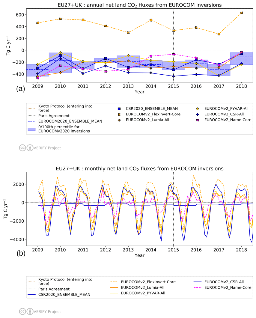
Figure A5 Annual (a) and monthly (b) time series for inversions in EUROCOM (Monteil et al., 2020). Inversions with solid lines were retained for the ensemble used in this work (shown in blue in the top figure for clarity). Note that the CSR values from EUROCOM have been replaced by the mean of four CSR simulations submitted under the VERIFY project (Appendix A1). Negative fluxes represent a sink for the land surface.

A5 Input data

A5.1 CRU ERA

The ERA5-Land (Muñoz-Sabater, 2019; Muñoz-Sabater et al., 2021) dataset at 0.1^∘ resolution over the global land surface at hourly resolution was aggregated to 3-hourly resolution and extracted for a 0.125^∘ grid over Europe (35^∘ N to 73^∘ N and 25^∘ W to 45^∘ E) to match the grid used in previous efforts within the VERIFY project. The variables extracted are the following: air temperatures, wind components, surface pressure, downwelling longwave radiation, downwelling shortwave radiation, snowfall, and total precipitation. From these, additional variables were calculated: total wind speed, specific humidity, relative humidity, and rainfall. Of these, the air temperature, downwelling shortwave radiation, specific humidity, and total precipitation were realigned with the CRU observation dataset (Harris et al., 2020) from 1901–2020 so that monthly means at 0.5^∘ pixels correspond exactly. Variation from observations is therefore present only on sub-monthly temporal scales and sub-0.5^∘ spatial scales. At the time of the model intercomparison, ERA5-Land was only available from 1981–2020. Consequently, the years 1901–1980 were taken from the UERRA HARMONIE-V1 dataset from ECMWF realigned with CRU observations under the VERIFY project and used in Petrescu et al. (2021). For both datasets, results were aggregated to daily and monthly temporal resolution for use as needed in some models.

A5.2 HILDA+

The full Hilda+ dataset is described in detail elsewhere (Winkler et al., 2020, 2021). Hilda+ is available at 1×1 km spatial and annual temporal resolution across the whole globe from 1960–2019 for six land use classes (urban, cropland, pasture/rangeland, forest, unmanaged grass/shrubland, and sparse/no vegetation). The algorithm uses Earth observation data and land use statistics to generate annual land use/cover maps and transitions. Probability maps for land use change categories are generated by using multiple Earth-observation-based data estimates of the extent of a given land cover category on a given pixel. The VERIFY project requires additional work to satisfy the needs of the various modeling groups. For example, the maps were extended back to 1900 to meet the needs of the DGVM groups. As observational data are lacking for the years before 1960, the temporal trend of the probability maps and the FAO land use database were used for extrapolation. In addition, forest areas were further subdivided into six forest types (Evergreen, needleleaf; Evergreen, broadleaf; Deciduous, needleleaf; Deciduous, broadleaf; Mixed; unknown/other) based on the ESA CCI land cover dataset (ESA, 2017). Spatiotemporal forest type dynamics within the forest category were included for 1992–2015. Before 1992 and after 2015, the static forest type distribution as found in the years 1992 and 2015 in the ESA CCI land cover was assumed, respectively.

A5.3 Nitrogen deposition

Wet and dry deposition maps of ammonium and nitrate covering Europe from 1995–2018 were calculated at 0.5^∘ spatial and monthly temporal resolution by the European Monitoring and Evaluation Programme (EMEP) MSC-W model (“EMEP model” hereafter). The EMEP model is a 3-D Eulerian chemistry transport model (CTM) developed at the EMEP center MSC-W under the framework of the UN Convention on Long-Range Transboundary Air Pollution (CLRTAP). The EMEP model has traditionally been used to assess acidification, eutrophication, and air quality over Europe, to underpin air quality policy decisions (e.g., the Gothenburg Protocol), and has been under continuous development, reflecting new scientific knowledge and increasing computer power. The model was described in detail by Simpson et al. (2012) and later updated as described in the annual EMEP status reports (Simpson et al., 2022, and references therein). For the VERIFY project, output from the EMEP model version rv4.33 was used (Simpson et al., 2019) and averaged to annual temporal resolution. In these simulations, the model was driven by meteorological data from the ECMWF IFS (European Centre for Medium-Range Weather Forecasts – Integrated Forecast System) version cy40r1. Land use data were taken from the CORINE land cover maps (De Smet and Hettelingh, 2001), the Stockholm Environment Institute at York (SEIY), the Global Land Cover (GLC2000) database, and the Community Land Model (Oleson, 2010; Lawrence et al., 2011). For more details, see Simpson et al. (2017).

A5.4 Coastal ocean fluxes

Ocean CO₂ fluxes were prepared for use as prior estimates in the regional inversions by combining the Rödenbeck global ocean estimate (Rödenbeck et al., 2014) with coastal ocean fluxes for Europe prepared under the VERIFY project. The combined dataset was prepared by choosing the coastal flux map when available and otherwise the open ocean map. The coastal ocean fluxes were generated for an area extending from the western Mediterranean to the Barents Sea and cover shelf areas down to 500 m water depth or 100 km distance from shore. First, surface ocean fCO₂ observations are taken from the annually updated SOCAT database (Bakker et al., 2016, 2022) and gridded to a monthly 0.125^∘ × 0.125^∘ grid. pCO₂ maps are created based on fitting a set of driver data (including sea surface temperature, mixed layer depth, chlorophyll concentration, and ice concentration) against the gridded fCO₂ observations. Both random forest and multi-linear regressions were used. The general procedure is described elsewhere (Becker et al., 2021), but for the version reported here, random forest regressions were used instead of multi-linear regression, and the region was extended to the south. The dataset was divided into seven subregions (Barents Sea, Norwegian coast, North Sea, Baltic Sea, Northern Atlantic coast/Celtic Sea, Southern Atlantic coast/Bay of Biscay, western Mediterranean), and each region was fitted separately (leaf size: 20, bag size: 500). The root mean square error (RMSE) of the random forest regressions was determined to be between 34 µatm (Baltic Sea) and 10 µatm (Barents Sea). Random forest regressions consist of many regression trees, each based on a random subset of data. Due to this internal structure, the overall RMSE can be seen as an out-of-box error estimate. The final fluxes are calculated from the pCO₂ maps with the atmospheric xCO₂ in the marine boundary layer and 6-hourly wind speed data using the gas transfer coefficient and the Schmidt number after Wanninkhof (2014), with the coefficient a_q of 0.2814 calculated after Naegler (2009) and 6-hourly winds from the NCEP-DOE Reanalysis 2 product (Kanamitsu et al., 2002).

Appendix B: Additional figures

B1 Overview figures

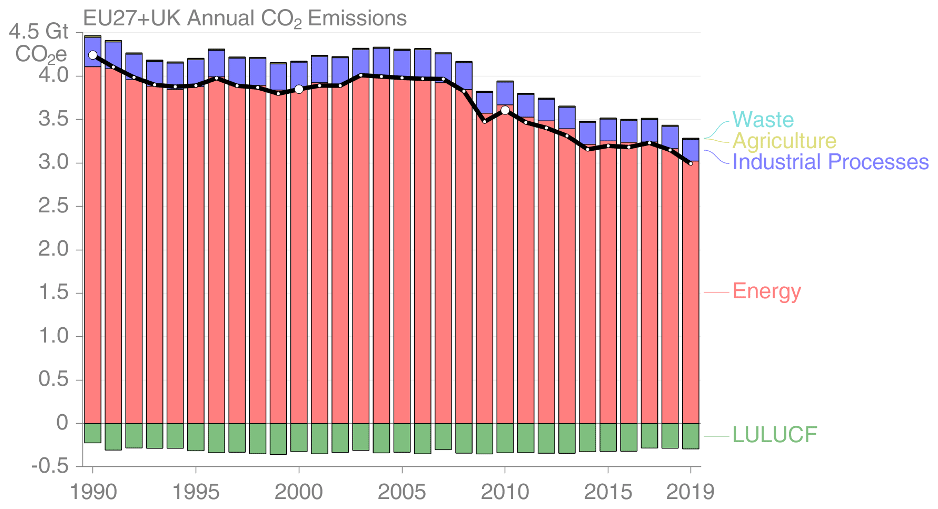
Figure B1 EU27+UK total annual GHG emissions from UNFCCC NGHGI (2021) with submissions split per sector.

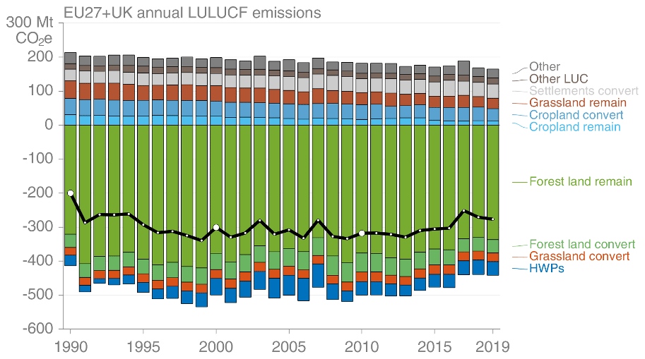
Figure B2 EU27+UK total annual GHG emissions from the LULUCF sector split into categories and subcategories, according to UNFCCC NGHGI (2021).

B2 CO₂ fossil

Figure B3 shows the CO₂ fossil emission estimates from EU27+UK split by major source categories for each dataset for a single year. Sectors 1, 2, 3, and 5 are included for the UNFCCC NGHGI (2021) total, without indirect emissions. A breakdown of the nine other fossil BU data sources corresponding to UNFCCC NGHGI sectors or categories is not currently available.

As in Andrew (2020), we observe good agreement for the EU27+UK between all BU data sources and the UNFCCC NGHGI (2021) data. The figure presents updated estimates for the year 2017, the most recent year when all datasets reported estimates. Sectors 1, 2, 3, and 5 are included for the UNFCCC NGHGI (2021) total, without indirect emissions.

While most datasets agree well on total emissions, there are some differences. Both BP and the EIA include bunker fuels and exclude most industrial process emissions. CEDS appears to be underestimating emissions from solid fuels, e.g., lignite in Germany and oil shale in Estonia. IEA's emissions are lower because they exclude most industrial processes. GCP's total matches the NGHGI exactly by design but remaps some of the fossil fuels used in non-energy processes from “Others” to the fuel types used. CDIAC, PRIMAP, and EDGAR v6.0 all report total emissions very similar to the UNFCCC NGHGI (2021). Larger differences are seen in the disaggregation of fuel types, generally because of differing definitions.

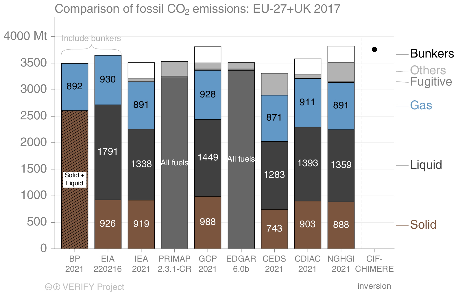
Figure B3 EU27+UK total CO₂ fossil emissions, as reported by nine bottom-up data sources (BP, EIA, CEDS, EDGAR v6.0, GCP, IEA, CDIAC, PRIMAPv2.3.1-CR, and the UNFCCC NGHGI (2021)) along with a top-down CIF-CHIMERE atmospheric inversion (black dot) (Fortems-Cheiney and Broquet, 2021). This figure presents the split per fuel type for the year 2017. “Others” is other emissions in the UNFCCC's IPPU, and international bunker fuels (the white boxes) are not usually included in total emissions at sub-global level. Neither EDGAR (EDGAR v6.0 provides significant sectoral disaggregation of emissions but not by fuel type due to license restrictions with the underlying energy data from the IEA.) (v6.0) nor PRIMAP publish a breakdown by fuel type, so only the total is shown. For BP, the method description allows for emissions from natural gas to be calculated from BP's energy data, but the data for solid and liquid fuels are insufficiently disaggregated to allow for replication of BP's emission calculation method for those fuels.

B3 CO₂ land

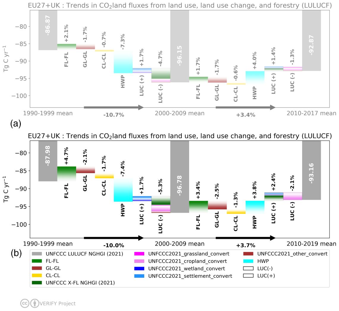
Figure B4 The contribution of changes (%) in CO₂ land fluxes from various LULUCF categories to the overall change in decadal mean for the EU27+UK as reported by member states to the UNFCCC. Panel (a) shows the previous NGHGI data from Petrescu et al. (2021), and panel (b) illustrates data from UNFCCC NGHGI (2021). Changes in land categories converted to other land are grouped to show net gains and net losses in the same column, with the bar color dictating which category each emission belongs to; note that the composition of the “LUC(+)” and “LUC(−)” bars can change between time periods. Not shown are emissions from “Wetlands Remaining wetlands”, “Settlements Remaining settlements”, and “Other land Remaining other land” as none of the BU models used distinguish these categories. The fluxes follow the atmospheric convention, where negative values represent a sink, while positive values represent a source. The color bars are shaded to guide the eye in the direction of the change (white to color).

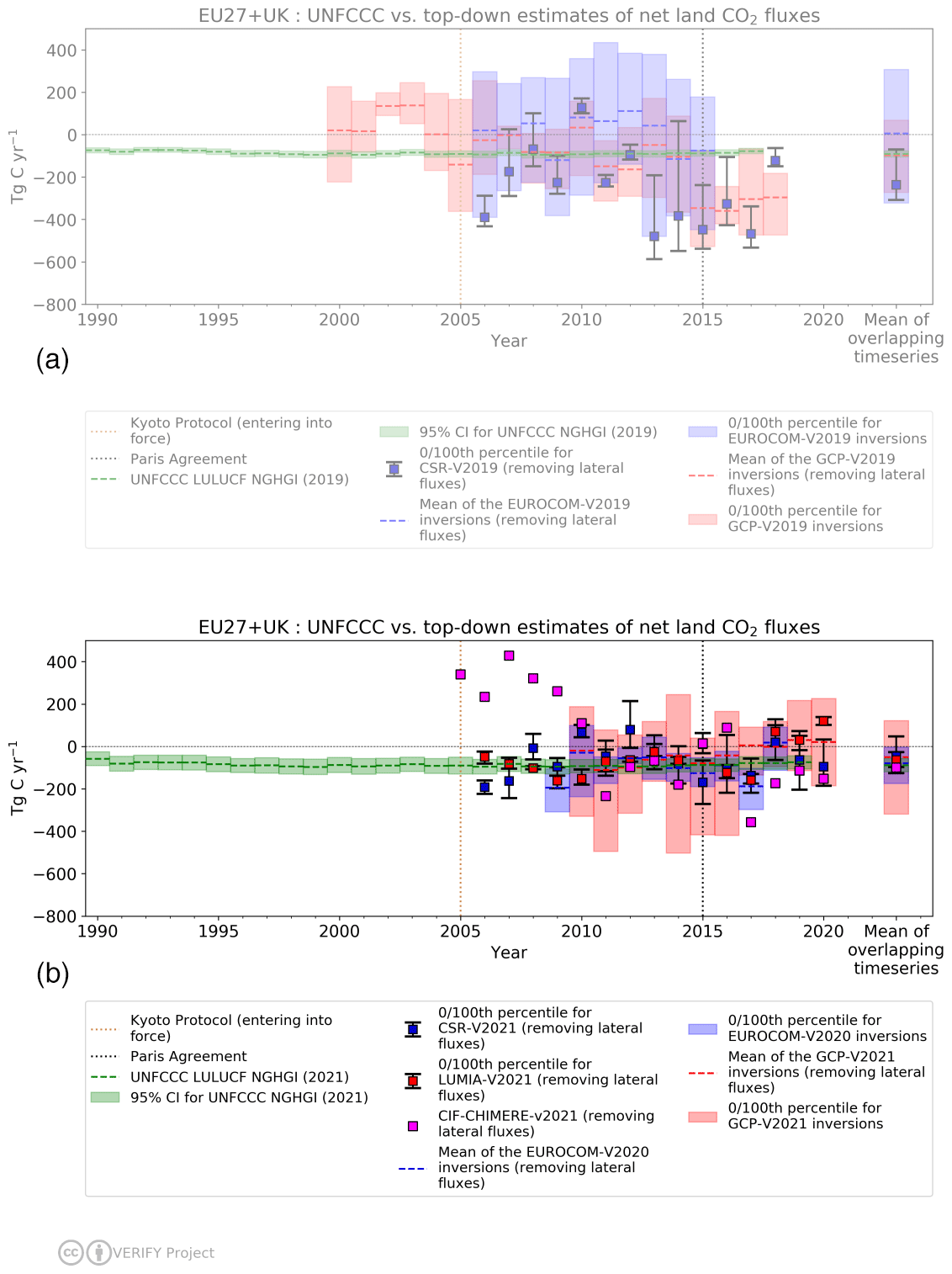
Figure B5 Comparison of inventories and atmospheric inversions for the total EU27+UK biogenic CO₂ fluxes from Petrescu et al. (2021) (a) and updated data from current study (b). Top-down inversion results are the following: the global GCB2021 ensemble, the regional EUROCOM ensemble, the regional CarboScopeReg model with multiple variants, the regional LUMIA model with multiple variants, and CIF-CHIMERE. The relative error in the UNFCCC values represents the UNFCCC NGHGI (2021) member states reported uncertainty computed with the error propagation method (95 % confidence interval) gap-filled and provided for every year of the time series. The time series mean overlapping period is 2010–2018. The colored area represents the min/max of model ensemble estimates. The same emissions due to lateral fluxes of carbon through rivers, crop trade, and wood trade are removed from the top-down estimates in both the top and bottom graphs for consistency. The fluxes follow the atmospheric convention, where negative values represent a sink, while positive values represent a source. Note that Petrescu et al. (2021) presented the top plot including a suite of bottom-up models, which have been removed here for clarity.

Appendix C: Source-specific methodologies – AD, EFs, and uncertainties

Table C1 Source-specific activity data (AD), emission factors (EFs), and uncertainty methodology for all current VERIFY and non-VERIFY 2021 data products.

NA – not available

Table C2 Comparison of the processes included in the inventories, bottom-up models, and inversions.

Not included: N, explicitly modeled: E, implicitly modeled: I, partly modeled: P. ^a UNFCCC and FAOSTAT are the ensemble of country estimates calculated with a specific methodology for each country, following some guidelines. ^b The climate effects can be estimated indirectly by CBM, using external additional input provided by other models. ^c EFISCEN-Space: increment is sensitive to weather but average weather. ^d EFISCEN only has production in cubic meter (m³) but does not have a direct HWP module. ^e Crop yield and residue harvest from cropland (20 % of residues harvested in case of cereals, no residue harvest for other crops). ^f EPIC-IIASA partly accounts for soil drought, i.e., plant growth limitation due to a lack of water in the soils. Heat stress and floods are not accounted for, though. ^g In principle, burning of crop residues on cropland can be explicitly simulated by EPIC-IIASA. However, it is not done for VERIFY as it is not a relevant scenario for the business-as-usual cropland management in Europe. ^h forest/cropland/grassland exist and have carbon stocks but have carbon fluxes only through change to management. FL-FL includes all land-use-induced effects (harvest slash and product decay, regrowth after agricultural abandonment and harvesting). ⁱ implicit by using observation-based carbon densities that reflect harvest/climate/natural disturbances. ^j peat burning and peat drainage are not bookkeeping model output, but are added from various data sources during post processing. ^k These categories are inputs to the inversions not a result; the inversions adjust the total land–atmosphere C flux, regardless of what went into the prior, and the posterior flux cannot really be disaggregated into contributions from separate processes. In a sense, as long as a process is sufficiently significant to influence the CO₂ observations, it will have an impact on the inversion results.