Estimating CO₂ emissions for 108 000 European cities

City-level CO₂ emissions inventories are foundational for supporting the EU's decarbonization goals. Inventories are essential for priority setting and for estimating impacts from the decarbonization transition. Here we present a new CO₂ emissions inventory for all 116 572 municipal and local-government units in Europe, containing 108 000 cities at the smallest scale used. The inventory spatially disaggregates the national reported emissions, using nine spatialization methods to distribute the 167 line items detailed in the National Inventory Reports (NIRs) using the UNFCCC (United Nations Framework Convention on Climate Change) Common Reporting Framework (CRF). The novel contribution of this model is that results are provided per administrative jurisdiction at multiple administrative levels, following the region boundaries defined OpenStreetMap, using a new spatialization approach. All data from this study are available on Zenodo https://doi.org/10.5281/zenodo.5482480 (Moran, 2021) and via an interactive map at https://openghgmap.net (last access: 7 February 2022​​​​​​​).

1 Background

While climate goals are set at the national and international level, it is often local governments and citizens who are most intimately involved in the accomplishment of these goals and who must adapt to the implied changes. The European Commission has been clear that cities will play a central role in reaching European climate goals. As with nation-states, a greenhouse gas (GHG) inventory is the first step to preparing a local climate action plan (CAP). Cities often use one of the various protocols available or develop their own methodology to create an emissions inventory. And this is for good reason – an inventory informs all levels of municipal decision making, from long-term planning strategies to infrastructure investments and day-to-day management of building permits. Nevertheless, many local governments in Europe still do not have a good estimate of their own GHG emissions. Establishing an emissions inventory is laborious and can be costly for jurisdictions that do not have in-house expertise. Hence, as the spotlight turns to cities to effect and manage a successful transition to carbon neutrality, many see the preparation and maintenance of a local emissions inventory as a considerable challenge.

Cities can develop their own inventories using a protocol such the Global Protocol for Community-Scale Greenhouse Gas Emissions Inventories (Fong et al., 2016), a joint initiative of the WRI (World Resources Institute), C40 (C40 Cities Climate Leadership Group), Global Covenant of Mayors for Climate & Energy, and ICLEI (International Council for Local Environmental Initiatives; Kona et al., 2021). An inventory informs all levels of municipal decision making, from long-term planning strategies to infrastructure investments and day-to-day management of building permits.

A number of GHG monitoring, reporting and verification (MRV) solutions have been put forward. These include sensor networks (both ground- and space-based) and a range of accounting and model-based approaches. No one of these approaches is ideal: they differ in terms of accuracy, precision, cost and scalability. In response it has therefore been suggested that MRV efforts should aim at triangulating true CO₂ emissions using a mix of empirical, modeling and statistical methods (Lauvaux et al., 2020; Mallia et al., 2020). The model presented here should be seen as one estimate, to be combined with other estimation approaches and local knowledge, to triangulate towards an actionable emissions inventory.

One approach for cities to monitor emissions is by using atmospheric measurement of GHG concentrations and “inverting” that for an emission quantity. These efforts require atmospheric transport models to translate the atmospheric mixing ratios into surface fluxes of GHGs (Davis et al., 2017; Ghosh et al., 2021). Concentration measurements can include dense, low-cost sensors (Kim et al., 2018), high-precision tower-mounted instruments (Turnbull et al., 2019; Whetstone, 2018), aircraft- and satellite-based measurements (NASA, 2021; Wu et al., 2020), the EU's CoCO2 and ICOS Cities (Integrated Carbon Observation System) projects, NASA's OSSE project (Observing System Simulation Experiment; Ott et al., 2017), and/or combinations of all of the above. By combining these approaches with high-resolution emission data products built using bottom-up approaches, attribution to emitting source by sector or fuel is possible and has shown good convergence (Basu et al., 2020; Lauvaux et al., 2020; Mueller et al., 2021).

Many estimates of emissions using techniques independent of atmospheric monitoring have also been accomplished. These inventory approaches are often described as being either “top-down” or “bottom-up” (though in fact models may use a combination of these approaches). Top-down models begin from national statistics, such as national energy use or fuel import statistics, while bottom-up approaches estimate emissions at the point of combustion or emission release based on deterministic information (e.g., fuel combustion characteristics, leak rates) and then aggregate these to an implied national total. The top-down approach uses spatial proxies such as gridded population, nighttime lights, gross domestic product (GDP) estimates and other available spatial proxy variables to allocate national total emissions across grid cells in each country. Bottom-up techniques often use a mixture of data such as direct flux monitoring (e.g., power plant stack monitors), local fuel or utility data, and traffic monitoring.

Several global- and country-scale spatially explicit GHG inventories have been developed based on either bottom-up or top-down approaches. The JRC EDGAR v6.0 (Joint Research Centre Emissions Database for Global Atmospheric Research; Crippa et al., 2020) and ODIAC (Open-Data Inventory for Anthropogenic Carbon dioxide; Oda and Maksyutov, 2011; Oda et al., 2018) inventories are well-established examples of global emission data products, but others have been developed (Andres et al., 1996, 2016b; Asefi-Najafabady et al., 2014; Nassar et al., 2013; Rayner et al., 2010; Wang et al., 2013), including some at the national/regional scale (Bun et al., 2019; Zheng et al., 2021a; Jones et al., 2021; Kurokawa et al., 2013; Meng et al., 2014). A number of these models use nighttime lights data as one input signal (or gridded population datasets, which in turn may be based on nighttime lights), though at least one study has found this is only moderately predictive (Gaughan et al., 2019).

Spatially explicit bottom-up GHG inventories have been accomplished at the regional, national and urban scale. For example, the US 1 km² hourly Vulcan CO₂ emissions data product (Gurney et al., 2020a, b, 2009) and the northeastern US 1 km² ACES (Anthropogenic Carbon Emissions System; Gately and Hutyra, 2018) data product. Similarly, work in Poland has achieved similar success (Bun et al., 2010, 2019). Building-/street-scale bottom-up efforts have also been accomplished with the HESTIA Project which has estimated hourly urban CO₂ data products in four US cities (Gurney et al., 2019, 2012; Patarasuk et al., 2016; Roest et al., 2020).

Finally, urban emissions have been estimated at the whole-city scale using both top-down and bottom-up techniques as individual city studies or as collections of urban areas (Ramaswami and Chavez, 2013; Chen et al., 2019a; Harris et al., 2020; Jones et al., 2021; Meng et al., 2014; Shan et al., 2018; Shan et al., 2017; Zheng et al., 2021a; Long et al., 2021) as well as results focused on city results in England (Baiocchi et al., 2015), China (Liu et al., 2020a; Wang et al., 2017) and Europe (Baur et al., 2015). Many of these studies extend analysis to include Scope 3 or consumption emissions.

Here we provide a new pan-European model estimating emissions at the municipality level (Moran, 2021). This is intended to be useful for cities which have not conducted their own inventory. The inventory disaggregates the totals from the official national CO₂ inventory, summarizing the 167 line items of the UNFCCC's (United Nations Framework Convention on Climate Change) Common Reporting Framework (hereafter, CRF) (IPCC, 2006) into nine emissions categories. The model identifies up to five levels of administrative hierarchy across 34 European nations including the UK.

This paper proceeds by first situating this contribution with respect to similar work. We then present the methodology and results, including a pixel- and city-level comparison with EDGAR and ODIAC and a first validation against 43 existing urban emissions inventories assembled by individual cities. We conclude with a discussion in which we reflect on use cases and next steps.

The JRC EDGAR database, ODIAC, and GCP-GridFED (Global Carbon Project gridded fossil emissions dataset) databases are obvious points of comparison to the model we present in this study. Section 3 presents a conceptual and numerical comparison of these datasets. The main innovations presented by this model over EDGAR and ODIAC are that (a) results are provided for administrative jurisdictions rather than on a raster grid and (b) the use of OpenStreetMap is novel. Additionally, our model is targeted to be useful to citizens and local governments, at the city level, by identifying the sources of their city's CO₂ emissions. This influences some of our modeling approaches, such as emissions attribution from ships and planes to ports and airports rather than along their physical voyage tracks. But it is the provision of ready-to-use results at the city, county and state level across Europe which we believe is the core contribution of this database.

The method described here is intended for creating an inventory of direct emissions. It is worthwhile to recall the distinction between Scope 1, 2 and 3 emissions inventories as defined in the WRI's Greenhouse Gas Protocol nomenclature (WRI et al., 2014). An inventory of direct emissions is called a Scope 1 inventory, a territorial emissions account or a production-based emissions account (PBA). A Scope 2 inventory will be largely identical to a Scope 1 inventory but reallocate the emissions from electricity production to the location where that electricity is directly used. A Scope 3 inventory, also called a footprint or a consumption-based account (CBA), will further expand the scope and attribute to consumers all emissions associated with imported goods and services produced domestically or abroad and emissions associated with waste exported outside the jurisdictional bounds. For urban areas with little production and much consumption, Scope 3 emissions can be substantial: studies estimate that for many urban cores their Scope 1 emissions are 30 %–50 % of their total Scope 3 footprint. Scope 3 inventories are estimated using trade and supply chain databases and rely on robust (i.e., well-modeled or empirically validated) Scope 1 inventories as a starting point. There is an active community working to prepare Scope 3 assessments at the city level (Chen et al., 2019b, a​​​​​​​; Heinonen et al., 2020; Minx et al., 2013; Moran et al., 2018; Pichler et al., 2017; Ramaswami et al., 2021; Wiedmann et al., 2021; Zheng et al., 2021b).

2 Methods

The approach presented here spatializes the national emissions inventory using activity data from OpenStreetMap (OSM), the EU's Emissions Trading System (ETS) registry of point source emitters and traffic data for airports. This method sums to a national total equal to the national inventory, generates results as both a gridded dataset and per administrative unit, and preserves detail on the sources of emissions. The intention is to best locate emissions to where they physically or legally occur.

As the spatial resolution of the inventory increases an interesting consideration emerges, namely that there is some discretion in where emissions should be spatially located. The emissions for a passenger ferry for example could be spatially located over water where they physically occur, at the office of the ferry company which is legally responsible, at an industrial harbor where the boat takes on fuel or at the passenger terminals where it traffics. At larger grid cell sizes these four locations are more likely to share the same grid cell, but with highly resolved models this becomes a modeling choice. Our choices on such decisions are documented in the relevant section of methods which describes each emissions category, but as a general principle we opt to locate emissions where it makes most sense for communication and outreach by those using the results, where policy tools are easiest to apply or where they physically occur, in that order.

The scope of coverage is the following: the model is currently built for the year 2018. This is the most recent year for which official national inventories were available from Eurostat (European Statistical Office) when the model was assembled. The list of countries covered is provided in the results section of this paper. The UK is included in the model. Regarding the impact of the UK's exit from the EU, we anticipate this will not substantially reduce the ability to use this model for the UK, since the UK has established its own UK ETS, and, we presume, will continue to publish an emissions inventory in CRF format. This study focuses only on CO₂ emissions; other greenhouse gases are not included. In each relevant section in Methods a discussion is included about how the model could be extended to handle other GHGs. One rationale for this choice is that the second-largest GHG, CH₄, is heavily driven by agricultural activities and rogue emissions, and these are some of the hardest to accurately spatialize. Furthermore, the intention in this study is to focus on fossil fuel use and not short-cycle carbon such as emissions related to land use and agriculture. Therefore, the model does not include emissions from land use, land-use change and forestry (LULUCF). The choice to exclude these from the model was based on considerations including that (a) estimates of total LULUCF emissions are often poorly constrained; (b) they are difficult to spatialize accurately; (c) local-government policies have fewer immediate policy options for managing these emissions; (d) national climate targets often exclude LULUCF emissions; and (e) there are diverse approaches to account for LULUCF and carbon sinks, leading to significant variability (Grassi et al., 2018; Petrescu et al., 2020).

The model assembly procedure can be summarized as follows. Further detail and discussion on each aspect is provided in the following subsections. First, emissions which can be attributed to point source facilities reporting under the ETS are separated from the national inventory. ETS-registered emissions are geolocated at the street address registered for that permit holder. In the cases where the location of emissions differs from the registered address (e.g., offshore oil activities or some company activities) this approach can still be rationalized, since (a) physically locating all facilities which are not at their mailing address will be difficult and (b) legally, the control of the emissions is likely at the registered address, so there is sense in calling attention to emissions which are controlled from there. Emissions from vehicles are apportioned equally to fuel stations as located in OSM. The model amortizes total national vehicle fuel use evenly across all fuel stations, though this will correctly neither capture subtleties such as fleet and trucking-only fuel depots nor differentiate between small (one to two pumps) stations and large filling stations with multiple pumps. Emissions which are associated with buildings (heating and cooling, construction, and light commercial activity), plus the residual industrial emissions which cannot be attributed to ETS sources, are apportioned equally onto all buildings registered in OSM. (OSM does allow for buildings to be tagged with extended attributes such as floor size, stories and use, but in our investigations <1 % of buildings use these attributes, so for now we have not attempted to utilize those fields.) Emissions from marine bunker fuels are apportioned equally to harbors as located in OSM (note that diesel fuel for small vessels will be treated as vehicle fuel). Emissions from aviation bunker fuel are spatialized onto airports proportional to the volume of passenger traffic handled at each airport, as reported by Eurostat. Fugitive emissions and emissions from petroleum byproducts are spatialized equally across national refineries and associated oil storage facilities. CO₂ emissions from farming and forestry are apportioned to farmed areas as located in OSM (these are based on the EU CORINE – Coordination of Information on the Environment – land-use map). Emissions from trains are mapped to passenger train stations.

Figure 1 displays the total emissions covered in the model, excluding LULUCF and carbon sinks, grouped according to the methods used to spatialize those emissions, and color-coded according to the approximate level of difficulty or degree of uncertainty of that spatialization, with grayer colors representing more easily spatialized emissions and brighter colors indicating emissions categories which, in the authors' experience, are more difficult to confidently spatialize.

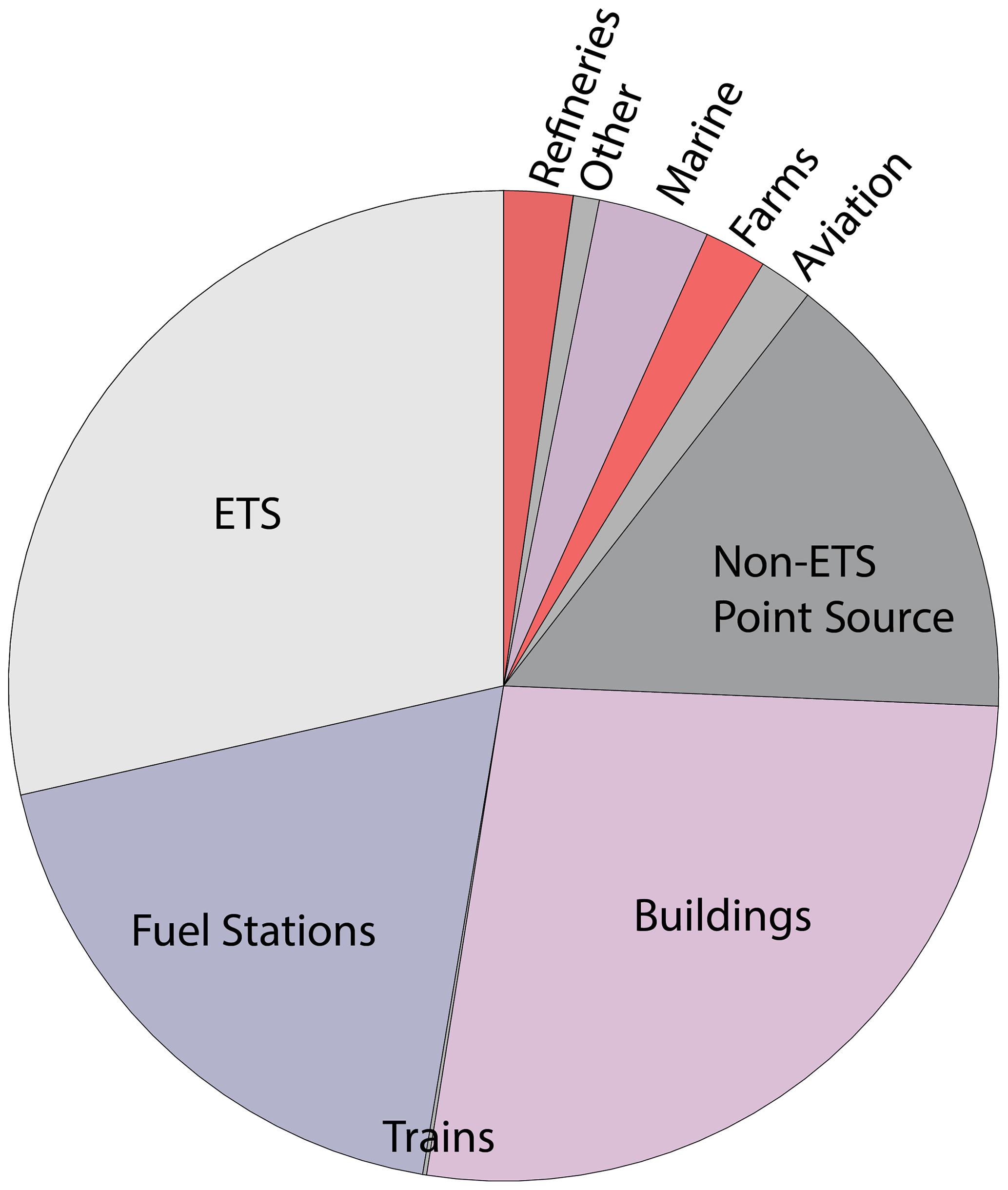
Figure 1 Composition of emissions across the 34 European countries covered. ETS shows the volume of emissions associated with ETS-registered point source emitters; fuel stations show emissions from vehicles; the “buildings” category comprises emissions from building heating, cooling, construction and light commercial activity. Non-ETS point source emissions is a residual category representing the difference between industrial emissions as reported in the national inventory and the sum of emissions reported by facilities participating in the ETS. Nearly half (42 %) of these occur in Turkey, which as of publication does not participate in the ETS, but this discrepancy is also observed in large emitters like Germany, France, the UK and Poland. These residual emissions are spatialized using OSM records instead of ETS addresses.

2.1 Mapping point source emissions regulated by the EU Emissions Trading System

The EU's Emission Trading System (ETS) requires large point source emitters to report emissions and report an address for every permit holder. A geolocation API (application programming interface) was used to translate these addresses into latitude–longitude coordinates. While for many facilities the address where the emissions are legally controlled is the same as the facility's physical address or in a nearby town, in some cases the two locations can differ more substantially (emissions from Norwegian offshore activities are largely legally controlled in the city of Stavanger, for example). The emissions associated with ETS-permitted facilities are then subtracted from the CRF inventory, thus leaving fewer total emissions remaining to be spatialized. The allocation of CRF emissions to ETS facilities is done as follows. For a number of CRF sectors (for example, “Fuel combustion in manufacture of iron and steel” (1.A.2.A)), some or all of the sector's emissions are attributable to ETS facilities. We constructed a priority-ranked concordance table to determine which CRF emissions are already covered by ETS-registered permits. Normally the ETS-reported emissions for a given activity are less than or equal to the CRF-reported emissions for that category, and there is only a small residual between the CRF-reported value and sum across pertinent ETS permits; however in some cases this residual is substantial.

The mapping between ETS categories and CRF categories is not always one-to-one. For example, the ETS uses the code “24: Production of pig iron or steel”. These facilities may correspond to the CRF activities, Fuel combustion in manufacture of iron and steel (1.A.2.A), Iron and steel production (2.C.1), or Ferroalloys construction (2.C.2). In our ranked concordance matrix approach, a rank of 1 is given to the first CRF activity; a rank of 2 is given to the second CRF activity; and a rank of 3 is given to the third CRF activity. The emissions from those ETS facilities from code 24 are first attributed to the rank 1 CRF activity until it is sated; then excess ETS emissions are assumed to come from the rank 2 activity until that volume is sated; the same for rank 3, and so on. Using the above example that could mean that all emissions under the first two CRF categories would be fully attributed to ETS iron and steel facilities and a portion of the emissions under rank 3, Ferroalloys construction (2.C.2), which cannot be attributed to ETS facilities, would remain to be spatialized.

In some cases it is unclear what the ranking of CRF activities should be. For example after allocating ETS emissions from “production of lime, or calcination of dolomite/magnesite” (ETS category 30) first to lime production (2.A.2) and secondarily to glass production (2.A.3), should excess ETS facility emissions from code 30 best be attributed to Cement production (2.A.1), Fuel combustion in manufacture of non-metallic mineral products (1.A.2.F), or Fuel combustion in other manufacturing industries and construction (1.A.2.G)? In this case the last three sectors are sated in smallest-to-largest order until no ETS emissions remain to be allocated. The rationale for the ascending sort order is that larger CRF categories will be easier to spatialize using other methods. In the earlier example of aluminum production, any surplus reported in ETS which exceeds the CRF reported aluminum production emissions is then assigned to the rank 2 CRF category of “Fuel combustion in other manufacturing industries and construction”, decreasing the amount of emissions in that CRF category which remain to be spatialized. We also note that not all facilities use the expected ETS activity code. For example we have observed some fertilizer plants reporting emissions under ETS activity code 42 “Other bulk chemicals” instead of activity 41 “Ammonia production”. Such misattributions can introduce distortions in the model results. To characterize the impact of these distortions the allocation of ETS emissions through the ranked priority allocation system into CRF would need to be followed manually in detail.

After linking ETS-reported emissions to the national inventory, the remaining CRF-reported emissions are spatialized using the methods described as follows.

2.2 Vehicles

These are emissions from the following five CRF categories:

• 1.A.3.B.i Fuel combustion in cars

• 1.A.3.B.ii Fuel combustion in light duty trucks

• 1.A.3.B.iii Fuel combustion in heavy duty trucks and buses

• 1.A.3.B.iv Fuel combustion in motorcycles

• 1.A.5.B Mobile fuel combustion sectors n.e.c.

These emissions are specialized according to the location of vehicle fueling stations as documented in OpenStreetMap. We make the assumption that the number of vehicle fuel stations in an area is proportional to the volume of traffic served. This is a simplifying assumption, and it is clearly communicated in the model presentation. In future development of the model, localizing vehicle emissions will be a top priority (for comparison, we note the Carbon Monitor project's use of TomTom live vehicle location data to spatialize traffic (Liu et al., 2020b)). This approach assumes that every fuel station supplies a similar level of vehicle traffic. It could be the case that some stations are small single-pump gas stations, while others are large facilities, for example such as those located along a major highway rest stop. To address this, one future solution could be introduce better road traffic estimates. While traffic load estimates are available for some roads, these estimates tend to be for only a few dozen specific highways. Fu and colleagues (Fu et al., 2017) proposed a method using neural networks to estimate vehicle flow on every road using OSM data and gridded population models. Osses et al. (2021) recently prepared a high-resolution map of emissions from vehicles in Chile. Better modeling of vehicle traffic, not only fuel station availability, would make the model more accurate in spatially estimating vehicle fuel emissions. Another potential solution would be to identify data on fuel station volume, e.g., sales estimates or number of pumps installed, but this may be challenging in practice. A second assumption is that every station serves a homogeneous mix of vehicles. It may be the case that some stations serve a specific fleet, for example a city bus fleet, and better identifying the mix of vehicles served by each fuel station would allow for the above five emissions categories to be more precisely spatialized. Insofar as electric-car adoption drives some fuel stations to close, the model will reflect lower vehicular emissions in areas with more electric vehicles. An interesting note is that in some urban centers light-truck traffic is suspected to be a larger emission source than passenger vehicles. Better distinguishing types of traffic and vehicles would be useful for helping guide decarbonization plans that are most appropriate for various areas.

2.3 Trains

Trains are a relatively minor source. Emissions for Fuel combustion in railways (1.A.3.C) were spatialized using passenger train stations as reported in OSM. Every train station was allocated an equal share of the total emissions. A limitation of this approach is that it may be that not all train traffic is equally fuel-intensive: some individual trains or sections of the rail network could be fully electrified, and other areas could not be. Another limitation is that the method allocates total train emissions (both passenger and cargo) equally across passenger stations, yet passenger stations are not all equally used, and cargo train activity would be more appropriately localized at freight yards. Reporting train emissions at passenger terminals does service a communicative value, as it reminds viewers that train traffic is not entirely emissions-free.

2.4 Buildings

In the following categories, only a portion of the emissions can be spatialized to ETS locations, but there remain emissions which must be spatialized onto buildings:

• 1.A.2.G Fuel combustion in other manufacturing industries and construction

• 1.A.4.A Fuel combustion in commercial and institutional sector

• 1.A.4.B Fuel combustion by households

• 1.D.3 Biomass – CO₂ emissions (memo item)

• 2.D.3 Other non-energy product use.

The largest shares of these remaining emissions are driven by building heating and cooling and fuel combustion by light industry and construction.

Correctly spatializing these emissions associated with buildings is a substantial challenge. OSM is sometimes known as “open buildings map”, since the database actually contains more buildings than streets. The OSM dataset reports an extensive number of buildings, but little data are available to characterize each building. OSM does not record all buildings. In many areas, including small towns, only a street address is marked, but there is no point or polygon data indicating what is built at that address. While it might be possible to obtain maps of all buildings from national cadaster agencies, part of our intention in the model is to develop methods which are replicable across other countries and do not rely on single-country datasets. Of the buildings recorded in OSM, only a small percentage (1 %–5 %, depending on the country) contain any information characterizing the building such as the number of floors, main usage activity, building material type or building age. Some recent offerings which provide building footprints (e.g., products from Maxar or Predicio building footprint data, free offerings from Bing/Microsoft, and academic initiatives such as coordinated through https://spacenet.ai, last access: 7 February 2022) could be used to identify at least the building footprint size and potentially height or construction material.

The approach used in the model is to apportion all of the emissions associated with buildings equally among all buildings and registered street addresses in each country. It is important to recall that for buildings heated by electricity, CO₂ emissions associated with electricity production will be located at ETS-registered power plants. As noted above, there is a paucity of information available by which we could further characterize building size or use.

2.5 Aviation

These total emissions are associated with kerosene used for aviation fuel (the sum of the CRF categories “Fuel combustion in domestic aviation” (1.A.3.A) and “International aviation” (1.D.1.A)) reported by EU member states and calculated compliant with IPCC (Intergovernmental Panel on Climate Change) 2006 guidelines (Maurice et al., 2006). These emissions are attributed to airports proportionally to total passenger kilometers (pkm). Fuel use from military aviation is excluded.

Total pkm data are derived from the combination of Eurostat statistics of route traffic and passenger traffic per airport. This procedure is preferred over an attribution based solely on total passenger or flight numbers, since we here implicitly incorporate information of both the flight length and aircraft size. These parameters are two major drivers for fuel consumption and emissions (Yanto and Liem, 2018).

2.6 Farming activity

The CRF uses the following three categories for farming-associated activities:

• 1.A.4.C Fuel combustion in agriculture, forestry and fishing

• 3.G Liming

• 3.H Urea application.

The largest of these, category 1.A.4.C, is challenging to spatialize for two reasons: first, the inclusion of fishing activity means emissions in this category overlap with emissions in marine traffic. To handle this, emissions from fishing would have to be estimated, removed from this amount and spatialized separately. Even then, the remaining emissions from fuel combustion in agriculture and forestry would still be difficult to spatialize. Second, we have not been able to identify a suitable dataset to use to divide and appropriately spatialize forestry as distinct from farming.

Our approach is to map these collected emissions onto locations of farmland as identified by the EU's CORINE land-use dataset, which is already incorporated into OSM. The above emissions were evenly allocated to the centroid points of all polygons tagged as farmland from CORINE. This approach will not correctly spatialize emissions associated with forestry. Also, this approach allocates the emissions evenly across every polygon tagged as farmland, regardless of the size of each patch. A future improvement could be to weight this allocation by patch size and thus assume every hectare of farmland is equally emissions-intensive to manage or to introduce activity-level data for agriculture, such as integrating maps of dairy cattle operations (Neumann et al., 2009) or similar.

As discussed in the Introduction, as well as in Sect. 2.10​​​​​​​ below on short-cycle carbon, currently the model intentionally excludes emissions from land use, land-use change, and biotic processes such as cattle digestion and manure handling.

The following categories in the CRF report also relate to farming:

• 3 Agriculture

• 3.1 Livestock

• 3.A Enteric fermentation

• 3.B Manure management

• 3.C Rice cultivation

• 3.D Managed agricultural soils

• 3.E Prescribed burning of savannas

• 3.F Field burning of agricultural residues.

2.7 Marine

Emissions from the maritime sector are part of international bunker fuel emissions together with international aviation. In both cases, emissions are calculated as part of the national GHG inventories but not included in national totals.

Emissions in this sector are comprised of the following CRF emissions categories:

• 1.A.3.D 4 Fuel combustion in domestic navigation

• 1.D.1.B 4 International navigation.

This covers tank-to-wake emissions that stem from fuel combustion. Total fuel consumption is calculated by a top-down assessment based on annual sales of bunker fuel in each country, comprising marine gas oil (MGO) and heavy fuel oils and distillates (HFO), and geospatially distributed across the 888 ports.

Port allocation of bunkered fuels is based on the total transport work for berth-to-berth ship voyages, as obtained from IHS Markit, totaling 773 000 port calls. Ship voyages are combined with their ship's respective average fuel consumption as reported by ship owners to the European Union's emissions monitoring scheme (EU MRV; monitoring, reporting and verification), given as kilograms of fuel per nautical mile. This covers all vessels operating in EU ports above 5000 Gt, totaling approximately 11 000 vessels. The distance covered with each voyage is calculated by applying Dijkstra's algorithm (Dijkstra, 1959) to find the shortest path between two ports, followed by a curve-smoothing process by the Ramer–Douglas–Peucker algorithm (Douglas and Peucker, 1973; Ramer, 1972). The average fuel consumption and distance sailed is used to estimate total bunker demand at the port level, by weighing the national reported bunker sales. This approach is expected to be gradually replaced by the bottom-up emission inventory provided by the MariTEAM (Maritime Transport Environmental Assessment Model) model (Kramel et al., 2021).

This assessment includes neither leisure crafts, considered negligible in comparison to cargo vessels; warships; naval auxiliaries; nor fish-catching or fish-processing ships that are exempt from reporting their activity to MRV.

2.8 Other

The following are some emissions which are difficult to spatialize:

• 1.C Transport and storage of CO₂ (memo item)

• 2.A.4 Other process uses of carbonates

• 2.D.1 Lubricant use

• 2.D.2 Paraffin wax use.

In the model these emissions are included in and spatialized using the same strategy as emission from buildings as described above.

2.9 Refineries

The following CRF emissions categories are associated with oil refineries and fossil fuel infrastructure:

• 1.B Fuels – fugitive emissions

• 1.B.1 Solid fuels – fugitive emissions

• 1.B.2 Oil, natural gas and other energy production – fugitive emissions

• 2.B.8 Petrochemical and carbon black production.

Carbon black, item 2.B.8, used to produce black ink, is a byproduct from fracking at refineries. Fugitive emissions (1.B.2) are by their nature difficult to spatialize (Plant et al., 2019). A number of studies in California have tried to characterize fugitive emissions from the aging oil wells and modern fracking equipment in the region (Hsu et al., 2010; Rafiq et al., 2020; Townsend-Small et al., 2012; Wennberg et al., 2012). In our model all fugitive emissions are attributed evenly across refineries and associated storage tanks as located in OSM. The fugitive emissions are apportioned equally among the buildings tagged (industrial as refinery) or (industrial as oil) in OSM. This approach has the disadvantage of not correctly spatializing fugitive emissions at the various wellheads and pumping and storage locations where such emissions physically occur but has the advantage of attributing fugitive emissions to refineries so that policy planning can recognize that fossil fuel creates emissions not only when it is combusted but also during its production. This approach follows the guiding philosophy of locating emissions where they best connect to the relevant policy discussion.

2.10 Land use, forestry, stock change and waste (short-cycle carbon)

Our model is focused on reporting CO₂ emissions from fossil fuel combustion and industrial processes. We explicitly set aside so-called “short-cycle carbon”, that is, carbon which is already in the biosphere stock. We limit the model to focus on emissions of carbon taken from the fossil stock.

Carbon put into sinks (under CRF table 5 – Waste), neither natural (terrestrial, aquatic or marine) nor man-made (e.g., timber construction or paper or biomass put into landfill), is spatialized or included in the results. Negative emissions from carbon capture and storage facilities are presently excluded from the model.

CO₂ emissions from CRF category 4, encompassing land use, land-use change and forestry, are also not included. Our intention is to spatialize fossil fuel combustion associated with agriculture and forestry but not emissions associated with landscape-scale soil and biotic processes. We reason that such landscape-scale emissions are both large and very challenging to address using locally available policy tools. Including them in a city-oriented plan, particularly in rural municipalities, could lead to a situation where the results are heavily dominated by an emissions category with few viable solutions.

In future iterations of the model it may be preferable to allow users to easily include or exclude the emissions in the model results. Currently our model does not include direct CH₄ emissions from cattle digestion and manure fermentation. This is a substantial emissions category with some remediation options, so it may be useful to include this in a future iteration of the model.

Another detail in this category is sewage treatment and landfills. These act as both sources and sinks of carbon. It is unclear whether net emissions from sewage plants and landfills are included inside the CRF category “Long-term storage of carbon in waste disposal sites” (5.F.1) or in another category. As category 5.F.1 is not included in the model, if net emissions from sewage are included in this category, those emissions will not be included in the model. Quantifying emissions associated with sewage treatment and local landfills would be an improvement to the model.

3 Benchmarking

We do not intend here to provide an exhaustive survey of available spatial emissions models. Here we only compare the OpenGHGMap model with some widely used global-level models. A full comparison of spatial emissions models, including several strong single-country models, would be a valuable contribution to the field but is not within the scope of the present paper. For one such comparison we refer to Hutchins et al. (2017).

Table 1 provides an overview and comparison of OpenGHGMap with ODIAC (Oda and Maksyutov, 2011), JRC's EDGAR (Crippa et al., 2020, 2019) and the Global Carbon Project's GCP-GridFED (Jones et al., 2021) spatial emissions models.

Table 1 Comparative overview of several spatial emissions datasets.

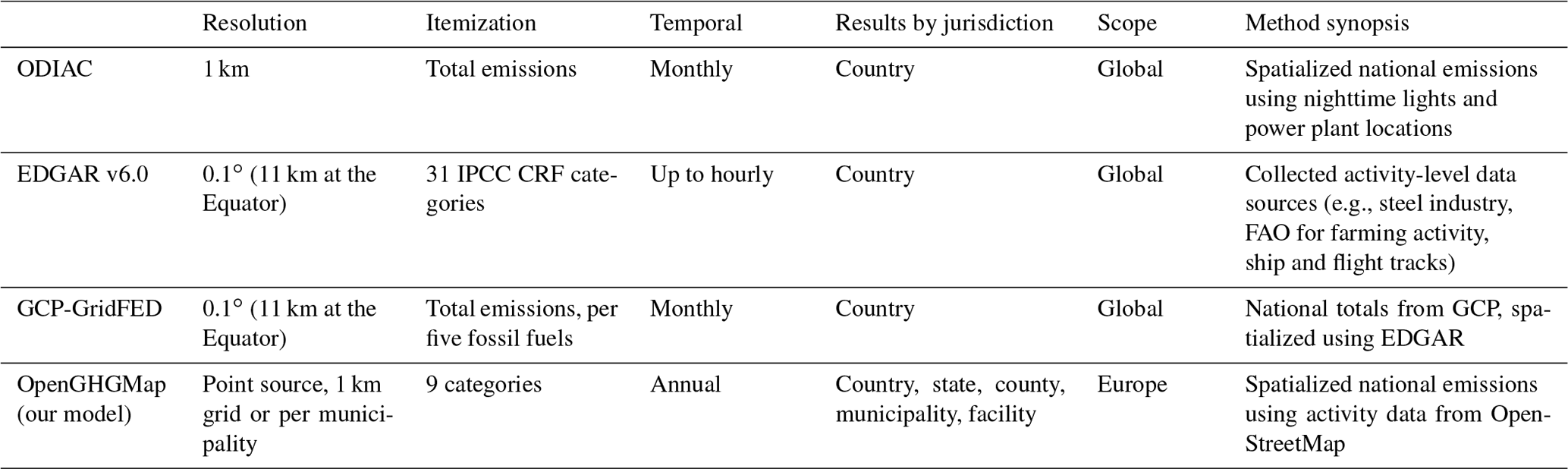
Regarding a comparison to EDGAR and GCP-GridFED, which uses EDGAR's spatialization layer, at the time of writing, the report with the methodology used for EDGAR v6.0 has not been published. Based on the data sources mentioned on the EDGAR website it appears that activity-level data have been obtained for various industrial activities (e.g., farming, fertilizer production, steel refineries, electricity generation), and plane and ship emissions are mapped to voyage tracks, but it is not published how emissions from buildings, light commercial activity and vehicles are spatialized, except that the GHS-POP (Global Human Settlement) gridded population dataset is mentioned. Since OpenGHGMap uses ETS facility-level data to map industrial emissions (an advantage afforded by its Europe-only focus), it may be that the two models will come to similar results for mapping industrial emissions, since presumably the activity-level datasets for industry used by EDGAR will be largely identical to the facility-level data from ETS. If EDGAR uses population density as a proxy to map vehicle and building emissions, this is a slightly different approach than OpenGHGMap's use of fuel stations and building locations from OSM.

Regarding a comparison to ODIAC, the original ODIAC was a ground-breaking project and introduced the approach of using power plant locations and nighttime lights as a proxy for emission activities. Since that project, more recent projects have introduced more proxy variables and activity inventories. In our results comparison (below) the ODIAC results still agree, but ODIAC does not present results with sector/activity detail which is important for further insight and to guide action.

In addition to this conceptual comparison of methods we also compare the numerical results. To compare the results of the OpenGHGMap model to ODIAC and EDGAR v6.0, the OpenGHGMap model was rasterized to a 30 arcsec raster (approximately 650 m² cells at 45^∘ latitude) to permit a direct cell-level comparison across emissions models and the GHS-POP gridded population model. The EDGAR dataset version is v6.0, data year 2018, with a native resolution of 0.1^∘ (360 arcsec) before re-gridding. For ODIAC, the model version is 2020, with data for 2018, with a native resolution of 1 km² cells. The three modeled inventories report slightly different totals for total European emissions. This is due to (a) differences in emissions categories covered; (b) for ODIAC, the monthly allocation; and (c) for EDGAR, the fact that in EDGAR, aviation and marine emissions are spatialized over ship and flight traffic routes rather than allocated to grid cells in the country. For this initial cross-model comparison, the three datasets were normalized to include only grid cells covered by all three models and then the total emissions across the three models were normalized so that we compare solely the spatial allocation. This is a simplified method for cross-model comparison and leaves considerable scope for future work on cross-model comparison. Our main aim here is to document this new model and conduct a preliminary validation, not conduct a robust cross-model comparison.

The cross-model cell-level comparison (Fig. 2) shows the degree of convergence between the OpenGHGMap and the EDGAR model. The OpenGHGMap reports more cells with low (<100 t CO₂ yr⁻¹) and very high (>1000 t CO₂ yr⁻¹) emissions. The OpenGHGMap model also reports higher cell-level variability than ODIAC: the ODIAC model reports that most cells have emissions in the range of 10²–10⁴, whereas the OpenGHGMap model reports cells with a range of 10¹–10⁵ t CO₂ yr⁻¹. This could potentially be an artifact due to the aggregation of ODIAC. The ODIAC model is natively provided at 1 km² resolution, corresponding to a cell size of 0.07–0.04 arcsec depending on latitude, and it could be that the aggregation to 30 arcsec cells for the purpose of comparison has masked higher variability within the 30 arcsec grid. Another hypothesis is that this homogeneity is due to ODIAC's use of nighttime lights data and that while illumination is relatively homogenous across urban and peri-urban areas, the emissions within similarly lit areas can be starkly different. Another noteworthy feature is that OpenGHGMap reports many more areas with low (<100 t) emissions compared to both EDGAR and ODIAC. One hypothesis is that this is related to the method of spatializing emissions from vehicle fuels to fuel stations. Since fuel stations often are spaced >650 m apart, especially in rural areas, this could result in many pixels in rural areas being assigned zero fuel emissions. As discussed elsewhere, the decision to localize vehicle emissions at fuel stations was a deliberate design choice in this model. Other models may choose to localize these emissions on roads or prorate them across a gridded population map on a per capita basis.

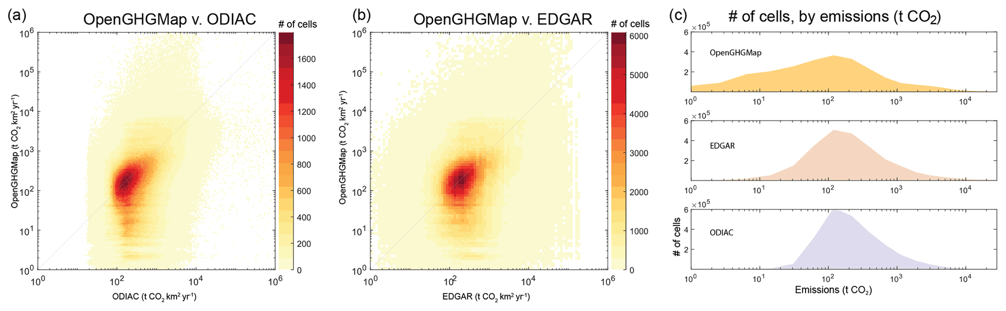
Figure 2 Emissions per standardized grid cell, cross-model comparisons and frequency analysis. Compared to the ODIAC dataset (a, c), OpenGHGMap reports higher cell-level variability ranging from 10¹ to 10⁵ t CO₂ yr⁻¹, while ODIAC reports most cells in the range of 10²–10⁴ t CO₂ yr⁻¹. Compared to the EDGAR v6.0 dataset (b, c), the OpenGHGMap dataset reports more cells with small (<10² t CO₂) emissions and fewer cells with high (>10⁴ t CO₂) emissions. The OpenGHGMap dataset reveals a higher variability in emissions per cell than do other models.

Next, we converted the administrative-region definitions from OpenGHGMap to a raster map compatible with the EDGAR v6.0 and ODIAC gridded datasets, and we compared the results aggregated by administrative level across the models at the city level (i.e., by city) across the models. We compared results both at the city level, i.e., at the highest level of regional detail per country, and at the county level, i.e., the administrative level one step above that. These results are presented in Fig. 3.

Figure 3 Cross-model comparison of CO₂ emissions per city (using the finest level of regional detail) and per county (using the next-finest level of regional detail per country).

Currently no methodology has been developed to quantify uncertainty in the model. In addition to being technically challenging, it is difficult to quantify uncertainty in any single portion of the model, much less the whole. Even if the national inventory or ETS inventory is taken to be 100 % reliable, errors and biases introduced during the various steps of spatializing these emissions are difficult to quantify. Developing a strategy for parameterizing reliability of model results would be a valuable next step in the research. Previous studies which have investigated techniques for parameterizing uncertainty in gridded spatial proxy models could be useful (Andres et al., 2016a; Bun et al., 2010; Hogue et al., 2016; Hutchins et al., 2017; Woodard et al., 2014).

3.1 Validation against city inventories

The main objective of the OpenGHGMap database is to provide easily accessible estimates for GHG emission inventories at the municipal level to assist local governments in developing more detailed inventories or in developing their own climate action plan (CAP). We compare our OpenGHGMap estimates for external validation with existing municipal GHG inventories compiled from a variety of sources in a dataset of 343 cities (Nangini et al., 2019). These emissions inventories are largely self-reported, are of varying quality and follow different protocols but still provide the most concrete point of comparison for our Scope 1 emissions estimates at the municipal level. In total, Scope 1 emission values for 44 European cities can be found in the database, which are compared to the OpenGHGMap estimates in Fig. 4.

Figure 4 Comparison between OpenGHGMap results and the community-level emissions inventories of 44 European cities. Color coding is used to indicate whether the city self-reports CO₂ or GHG (CO₂eq) emissions. Since OpenGHGMap reports only CO₂ emissions, this is limited to an indicative comparison, not a precise comparison.

The figure shows very high agreement (Pearson correlation coefficient of 0.937), despite the different methods and timing of the city inventories (emission years between 1994 and 2016 with a median of 2013). Only Ravenna, Italy, differs by several orders of magnitude, but the value in the 343-city database is not realistic (11 kt CO₂ for a population of 150 000 is unrealistically low).

4 Main findings

4.1 Results overview

An overview of the results for Europe is shown in Fig. 5. The results are presented both in absolute and per capita terms. Some noteworthy features are the high emissions in the coastal Netherlands, associated with marine activity, and the high emissions from the island of Gotland in the Baltic Sea, driven by one large cement facility there. Emissions in France are remarkably concentrated into a few, primarily coastal, cities.

One limitation which must be kept in mind when looking at the results at the municipal level is that municipalities vary in size between countries. In continental Europe municipalities are quite small, while in the Scandinavian countries the most local administrative units are relatively large and thus aggregate more emissions and are more visually prominent. For some analyses, gridded maps, where the spatial unit of analysis is consistent, are preferable to political maps.

Population per administrative area was estimated by overlaying the administrative boundary on the GHS-POP gridded population map. Gray areas indicate areas where no model results are available. In some cases (as seen for example in Ukraine and Romania) the administrative regions at that level are not exhaustive.

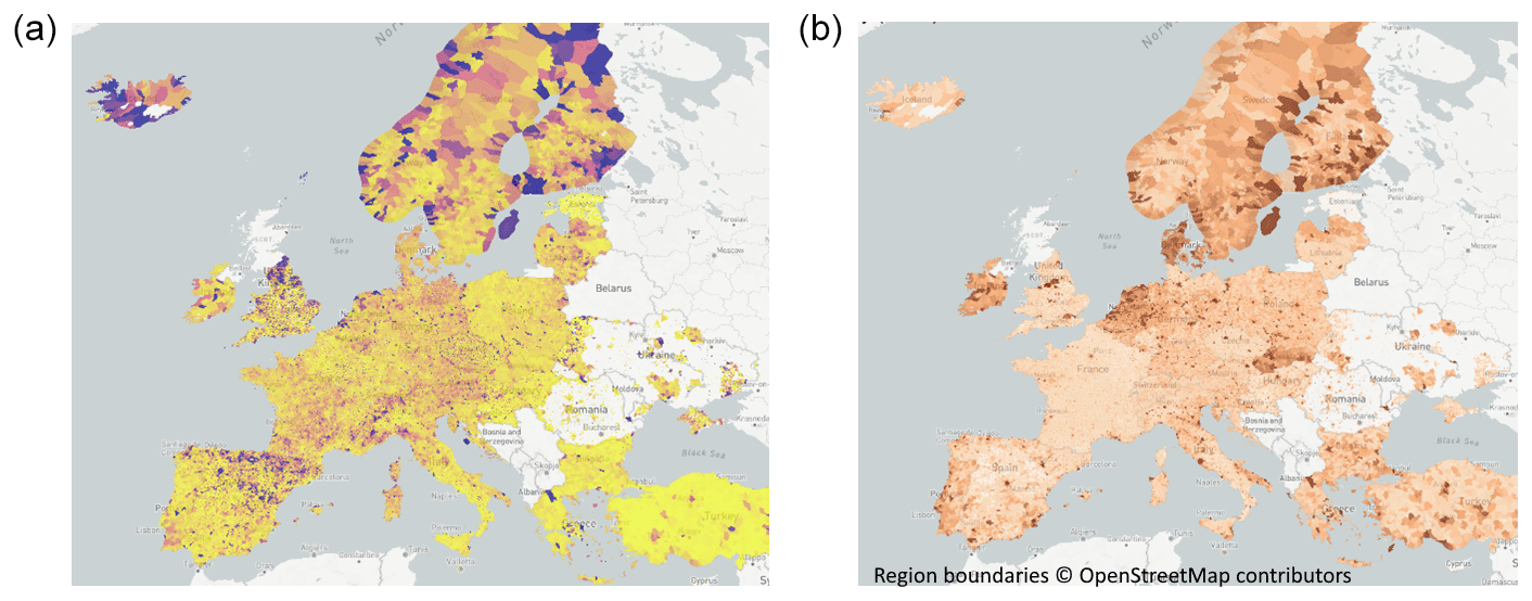
Figure 5 OpenGHGMap.net website screenshots. CO₂ emissions per municipality in absolute terms (a) and per capita terms (b). Darker colors (browns, purples) indicate higher emissions (absolute values can be found at the website http://openghgmap.net, last access: 7 February 2022). Base map © OpenStreetMap contributors 2022. Distributed under the Open Data Commons Open Database License (ODbL) v1.0.

In many countries, emissions are remarkably concentrated in a few regions. As seen in Fig. 6, in 21 of the 34 countries assessed, >30 % of national emissions arise from 10 municipalities. This implies that focused changes in a few political regions could contribute substantially to achieving national reduction targets.

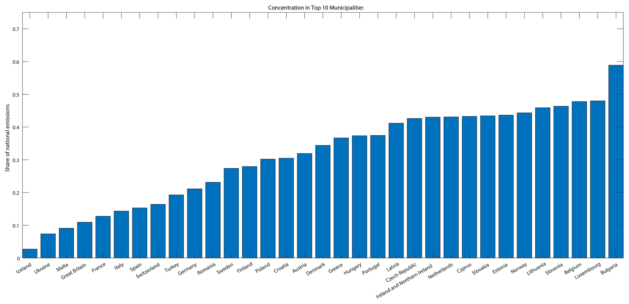
Figure 6 Share of national emissions arising from the top 10 emitting municipalities (or smallest finest administrative distinct) in each country. (Liechtenstein is not shown because the country only has 11 municipalities.)

The important role of high-emitting municipalities is seen at the European level as well. Figure 7 presents a Lorenz curve showing the contribution of municipality to the total European emissions. A striking degree of concentration is visible, with 10 municipal regions across Europe driving 7.5 % of emissions, 100 driving 20 % and the top 10 cities in each country collectively driving 33.4 % of total European emissions. These highest-emitting regions are not necessarily the most populous, since in many cases outlying industrial facilities are major drivers of emissions.

Figure 7 Lorenz curve showing the cumulative contribution to total emissions from each municipality.

4.2 Case study of Norway

To demonstrate the results provided by the model, we investigate Norway as a case study. In Norway there are just two levels of administrative hierarchy: counties (fylke) and municipalities (kommune), corresponding to the NUTS-2 and NUTS-3 (Nomenclature of Territorial Units for Statistics) levels respectively. This is a relatively simple configuration; for many European countries the system of administrative hierarchy is complex and deeply historical. For example in Germany some cities are peers with states, and the administrative configuration is slightly different between states (in some states there is a level 7 administrative subdivision, while in other states there is not); in Switzerland not all cantons use subdivisions; and in some places, statistic agglomerations of areas, such as capital cities with their suburbs, may be more relevant than the judicial regions. Our model provides results at all administrative levels in a country as defined in OSM. There are up to 10 levels available (we do not include level 11, which is for neighborhoods and parishes), and most countries use between levels 2 and 5.

The results for Norway at the NUTS-2 (fylke) level (Fig. 8) show concentration and highlight the importance of industrial sources in Norway. The fylke of Rogaland is the highest emitting. This is because in Stavanger, a city in Rogaland known as “the oil capital of Norway”, in addition to reported emissions from petroleum facilities physically around the city, many of the ETS-registered point source emissions from offshore facilities are legally registered to company offices in Stavanger.

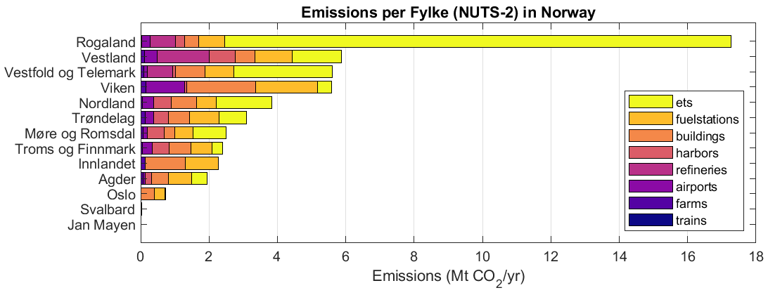
Figure 8 CO₂ emissions per NUTS-2 region (fylke) in Norway. The very high emissions in Stavanger (Rogaland) are driven largely by ETS-registered point sources. Stavanger is known as the oil capital of Norway. Note that the fylke of Oslo itself is small (ranked 11th), coextensive with only the heart of the city, and that Viken (ranked 4th) is the region which encompasses the greater Oslo region.

Viken, the region of greater Oslo, has 5.8 Mt of CO₂ emissions. The model results show that 32 % of these emissions come from vehicles and 36 % from buildings. Fossil fuel heating has been phased out of most buildings in Norway, so these emissions are from light commercial activity, such as small burners, boilers and generators not reporting to the ETS. A full 20 % of emissions in Viken (1.1 Mt) are associated with Norway's largest airport, the Oslo Airport at Gardermoen. As described in Methods, total emissions from aviation bunker fuel use in the country are allocated across airports in the country, prorated by 2018 passenger volume. This approach could be biased, and emissions from cargo flights, long-haul flights and military aviation should be located at airports different from those handling the most passenger traffic. This is a limitation of the current model.

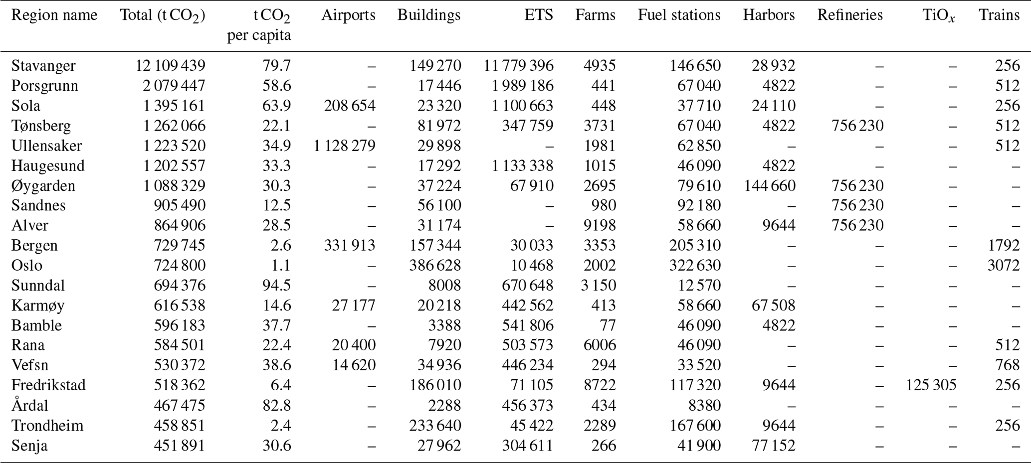
Table 2 presents results at the municipality (kommune, or LAU-1; local administrative unit) level for the top 20 municipalities. The relatively low emissions from the cities of Oslo (ranked 11th), Bergen (ranked 10th) and Trondheim (ranked 19th) is surprising given these are the three largest cities in Norway. Industrial emissions from ETS sources are the primary emissions drivers for the top four cities. The city-level results do also reveal some challenges with the model. The “refineries” category is defined as the residual between the national total emissions associated with industrial facilities and the total reported by the ETS facilities, and this residual is allocated evenly across facilities tagged as refineries in OSM. Overall this residual is small, but since there are few refineries, for individual cities it is substantial. Also noteworthy are the major emissions from harbors in the residential island archipelago of Øygarden. Currently emissions from marine bunker fuel are allocated evenly across all facilities tagged as “harbor” in OSM. In Øygarden there are many small-boat facilities, often not even selling fuel, yet at the same time the island region outside of Bergen is also heavily trafficked by large offshore work ships and cargo ships. Improving the methods used for spatializing emissions from marine bunker fuel use would help improve the model for Norway and other countries with extensive marine traffic.

Table 2 Estimated CO₂ emissions for 2018 for the top 20 emitting municipalities in Norway, as generated by OpenGHGMap.

The model can be explored as tabular data or as a gridded raster model or visualized on a map. Figure 9 provides an overview of the distribution of emissions across Norway, aggregated at the county and municipality levels. A concentration of emissions in Stavanger (in the southwestern corner) and Porsgrunn (an industrial area in the south) is clearly visible.

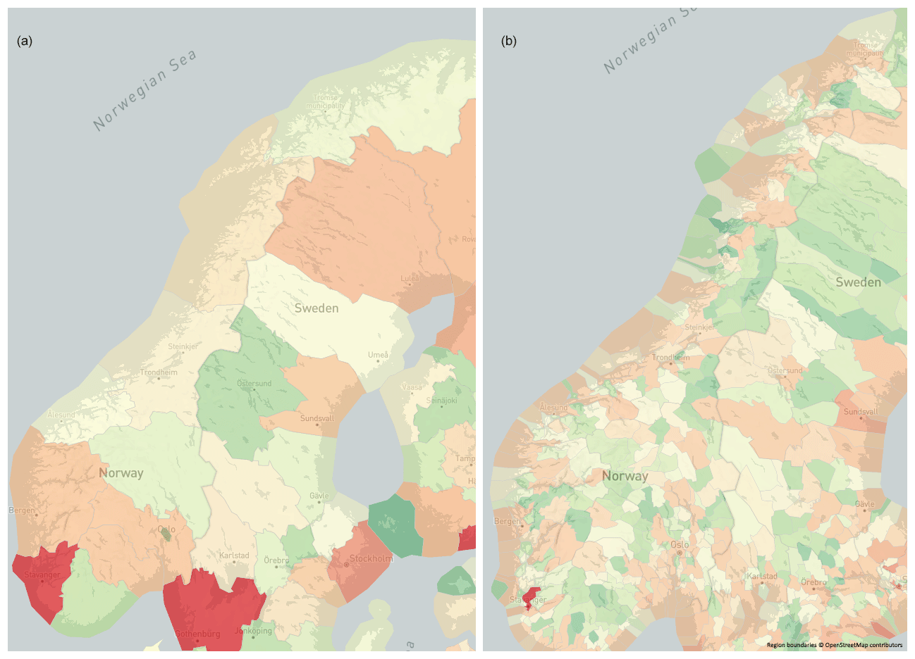
Figure 9 Screenshot of the website heatmap visualization of OpenGHGMap-estimated CO₂ emissions at the NUTS-2 county level (a) and municipality level (b) in Norway. Regions are color-coded from green to red for the lowest to highest-emitting region in the country. Base map © OpenStreetMap contributors 2022. Distributed under the Open Data Commons Open Database License (ODbL) v1.0.

Internally, the model attributes all national emissions to points across the country. It is possible to zoom in and view these emission point sources. Figure 10 provides a screenshot from the model visualization for the city of Trondheim, a city of 200 000 located in central Norway. The dots over each building, farm, fuel station and ETS facility are scaled according to the estimated amount emissions coming from that point. Orange dots show ETS-registered facilities. Purple dots in the figure show fuel stations. The fine gray dots in the figure show all buildings registered in OSM. As detailed in Methods, emissions from several categories are allocated to buildings. The use of fossil fuel for building heating is extremely rare in Norway. The emissions in the building category in Norway are mostly from light commercial activity: boilers, generators, ovens and the similar emissions from light commercial activity which are below the ETS reporting threshold. As discussed above, it is difficult to characterize buildings (e.g., buildings as different as a hospital, mall, auto body shop and small cottage are not distinguishable, nor can mansions be differentiated from cottages) (Milojevic-Dupont et al., 2020), but this is clearly a frontier where further work is merited.

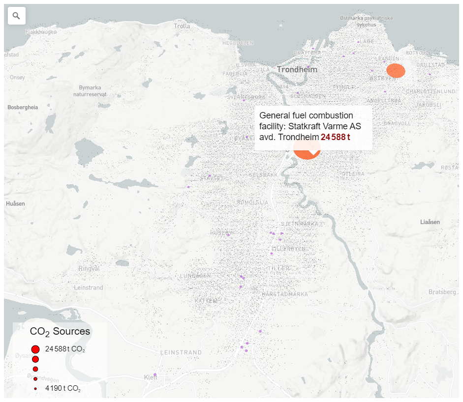
Figure 10 Example visualization of spatialized CO₂ emissions inventory for Trondheim, a city of 200 000 in central Norway, and the surrounding region. Small gray dots represent individual buildings; purple dots are emissions from fuel stations; and the large orange dots are ETS-registered point source facilities (a waste incineration plant and a factory making mineral wool). This detailed view, while only an estimate, can provide residents and government agencies a thought-provoking view of what decarbonization will look like for their town.

5 Code availability

The source code is not available at the time of writing. The authors plan to clean up the code and prepare a publicly usable version in the future. This will be linked on the Zenodo data repository and project website (https://doi.org/10.5281/zenodo.5482480, Moran, 2021).​​​​​​​

6 Data availability

Datasets are available via Zenodo at https://doi.org/10.5281/zenodo.5482480 (Moran, 2021).

The model website, with an interactive map, is https://openghgmap.net (last access: 7 February 2022​​​​​​​).

7 Limitations, uncertainties and future work

One limitation of the approach presented in this paper – and a potential source of difficult-to-detect bias – could be inconsistent coverage in OpenStreetMap. As OSM is a crowd-sourced dataset, there is no assurance of homogeneous coverage. Some areas of the country may be well-covered in OSM and others only sparsely (Hecht et al., 2013). This could introduce biases such as underreporting the number of fueling stations and thus underestimating vehicle traffic. The authors are not aware of any effort to characterize the consistency of OSM coverage; this would be a valuable next step both for the work presented here as well as for the OSM project and work derived therefrom.

For countries which do not participate in the ETS and do not have a similar domestic MRV system for large point source carbon emitters, spatializing emissions from point source polluters will be a challenge. Resources such as OSM and the Global Power Plant Database, which have considerable information at the facility level (e.g., output in megawatts and fuel source for power plants), could be of use.

The spatialization of emissions from vehicles and buildings – the two largest emissions categories – is challenging. The assumption in OpenGHGMap that every fuel station serves an equal volume and mix of vehicles is simplistic. The lack of even basic data characterizing buildings by height, area, age or material makes it impossible to differentiate buildings as varied as a terrace house block, separated house, mall or hospital. Some novel approaches for characterizing building stocks have recently been proposed (Haberl et al., 2021; Milojevic-Dupont et al., 2020; Peled and Fishman, 2021) which could be used. Developing more accurate town-level models of building emissions may require different modeling approaches, such as utilizing data from national building cadaster registries or from advanced remote sensing datasets such as from synthetic aperture radar satellite constellations, airborne lidar sensors, and machine learning used with mobile airborne or ground cameras.

OpenGHGMap treats the CRF National Inventory Reports (NIRs) as authoritative. However, these inventories contain uncertainties. The NIR reports provide annexes which discuss uncertainties at the sector, sub-sector and activity levels. The current version of the OpenGHGMap model does not exploit this uncertainty information, but future versions may. At the present time OpenGHGMap focuses on spatially distributing the reported national emissions totals and limits uncertainties to that spatialization exercise rather than including also the uncertainties within the NIR itself. Related to this it is noteworthy to mention related work on intercomparison of national emissions totals (Elguindi et al., 2020) and an assessment of uncertainty in the bottom-up EDGAR v6.0 model (Solazzo et al., 2021). Since OpenGHGMap treats national inventories as a fixed constraint with no uncertainty, the sources of uncertainty in the model are purely related to the spatialization of emissions. These uncertainties, as well as modeling choices, are discussed in the relevant section of Methods above.

Our emissions inventory can support local authorities in their journeys towards climate neutrality in multiple manners. The inventory can help make local and regional sources of emissions more tangible for diverse politicians, city administrations and local communities and provides a good starting point, especially for communities that lack a detailed GHG emissions inventory. Making an abstract concept such as greenhouse gas emissions more visible will enable discussions regarding the localization and upgrading of facilities and infrastructures and will provide a basis for emblematic changes with a high impact potential for the region. Connecting the inventory to digital urban twins with detailed information regarding built environment characteristics may help overcome the current limitations of lack of building data.

In order to further develop the model, we will actively discuss and test it with local authorities to fine-tune it to their needs in order to make informed decisions. Furthermore, we will explore how we can further refine data collection, analysis and spatialization through the use of a geographic information system (GIS) combined with crowdsourcing and citizen science.

We foresee a number of use cases for the results presented here. For one, many local governments in Europe do not have an emissions inventory. The estimated inventory presented here presents a baseline initial estimate. This can be used to reveal which are the priority areas for reduction in each locale. For example, while vehicle electrification is highly promoted, it could be the case that for some regions emissions from residential or commercial buildings or industrial sources are multiple times higher than from private cars and thus represent more important reduction opportunities. The results presented here are not a full replacement for an inventory prepared using a tool like the GHG Protocol for Cities. A bespoke inventory will be more detailed, but the approach presented here can act as a starting point, help with classifying emissions and provide a benchmark against which estimates can be compared or even calibrated. The process of preparing the inventory itself usually triggers discussions about solutions. As the body of solutions grows it is possible to imagine cities soon being able to construct a climate action plan based on a menu of options. An estimated inventory like the one presented here could be used to prioritize or filter a longer list of solutions into the shorter set most suitable for each city. Finally, the results presented here have some communication value. There is much discussion about decarbonization at the national and EU level, but many are curious about what this should look like at their town, building or business level. The results presented here can help people translate macro-level concerns into a more tangible vision of what should change in their hometown and how they can participate in that transition.

To conclude, we present a new European emissions inventory which disaggregates national CO₂ inventories to city- and county-level administrative jurisdictions. The model is broadly consistent with the ODIAC and EDGAR results but shows higher cell-level variability and provides results per jurisdiction rather than in a gridded form. The estimated inventories provided by this model can help local governments begin establishing an emissions inventory.