the Creative Commons Attribution 4.0 License.
the Creative Commons Attribution 4.0 License.
 | 18 Feb 2022
Design and description of the MUSICA IASI full retrieval product
Matthias Schneider
Benjamin Ertl
Christopher J. Diekmann
Farahnaz Khosrawi
Andreas Weber
Frank Hase
Michael Höpfner
Omaira E. García
Eliezer Sepúlveda
Douglas Kinnison
IASI (Infrared Atmospheric Sounding Interferometer) is the core instrument of the currently three Metop (Meteorological operational) satellites of EUMETSAT (European Organization for the Exploitation of Meteorological Satellites). The MUSICA IASI processing has been developed in the framework of the European Research Council project MUSICA (MUlti-platform remote Sensing of Isotopologues for investigating the Cycle of Atmospheric water). The processor performs an optimal estimation of the vertical distributions of water vapour (H2O), the ratio between two water vapour isotopologues (the ratio), nitrous oxide (N2O), methane (CH4), and nitric acid (HNO3) and works with IASI radiances measured under cloud-free conditions in the spectral window between 1190 and 1400 cm−1. The retrieval of the trace gas profiles is performed on a logarithmic scale, which allows the constraint and the analytic treatment of ln [HDO]−ln [H2O] as a proxy for the ratio. Currently, the MUSICA IASI processing has been applied to all IASI measurements available between October 2014 and June 2021 and about two billion individual retrievals have been performed.
Here we describe the MUSICA IASI full retrieval product data set. The data set is made available in the form of netCDF data files that are compliant with version 1.7 of the CF (Climate and Forecast) metadata convention. For each individual retrieval these files contain information on the a priori usage and constraint, the retrieved atmospheric trace gas and temperature profiles, profiles of the leading error components, and information on vertical representativeness in the form of the averaging kernels as well as averaging kernel metrics, which are more handy than the full kernels. We discuss data filtering options and give examples of the high horizontal and continuous temporal coverage of the MUSICA IASI data products.
For each orbit an individual standard output data file is provided with comprehensive information for each individual retrieval, resulting in a rather large data volume (about 40 TB for the almost 7 years of data with global daily coverage). This, at a first glance, apparent drawback of large data files and data volume is counterbalanced by multiple possibilities of data reuse, which are briefly discussed. Examples of standard data output files and a README .pdf file informing users about access to the total data set are provided via https://doi.org/10.35097/408 (Schneider et al., 2021b). In addition, an extended output data file is made available via https://doi.org/10.35097/412 (Schneider et al., 2021a). It contains the same variables as the standard output files together with Jacobians (and spectral responses) for many different uncertainty sources and gain matrices (due to this additional variables it is called the extended output). We use these additional data for assessing the typical impact of different uncertainty sources – like surface emissivity or spectroscopic parameters – and different cloud types on the retrieval results. The extended output file is limited to 74 example observations (over a polar, mid-latitudinal, and tropical site); its data volume is only 73 MB, and it is thus recommended to users for having a quick look at the data.
- Article
(19174 KB) - Full-text XML
- BibTeX
- EndNote


The IASI (Infrared Atmospheric Sounding Interferometer, a thermal nadir sensor; Blumstein et al., 2004) instrument aboard the Metop (Meteorological Operational) satellites presents possibilities for measuring a large variety of different atmospheric trace gases (e.g. Clerbaux et al., 2009) with daily global coverage. Because each Metop is an operational EUMETSAT (European Organization for the Exploitation of Meteorological Satellites) satellite, IASI measurements offer excellent global daily coverage and a sustained long-term perspective (measurements of IASI and IASI successor instruments are guaranteed between 2006 and the 2040s). This provides unique opportunities for consistent long-term observations and climate research.
In addition to humidity and temperature profiles (which are the meteorological core products; August et al., 2012), IASI can detect, for instance, atmospheric ozone (O3; e.g. Keim et al., 2009; Boynard et al., 2018), carbon monoxide (CO; e.g. De Wachter et al., 2012), nitric acid (HNO3; Ronsmans et al., 2016), nitrous oxide and methane (N2O and CH4; De Wachter et al., 2017; Siddans et al., 2017; García et al., 2018), the ratio between different water vapour isotopologues (Schneider and Hase, 2011; Lacour et al., 2012), and different volatile organic compounds (Franco et al., 2018).
These diverse opportunities of IASI together with the good horizontal and daily coverage result in a large number of IASI products generated in the context of often computationally expensive retrievals. In order to ensure the ultimate benefit from these efforts, the generated data should be FAIR (e.g. Wilkinson et al., 2016): findable, accessible, interoperable, and reusable.
During the European Research Council project MUSICA (MUlti-platform remote Sensing of Isotopologues for investigating the Cycle of Atmospheric water, from 2011 to 2016) we developed at the Karlsruhe Institute of Technology a processor for the analysis of the thermal nadir spectra of IASI. Here we present the MUSICA IASI trace gas processing output, which encompasses vertical profiles of H2O, δD (, with Vienna Standard Mean Ocean Water, VSMOW, of ), N2O, CH4, and HNO3. In addition to the retrieved trace gas profiles, the processing output consists of a comprehensive set of variables describing the retrieval settings and product characteristics for each individual retrieval.
Figure 1 shows a schematic of the MUSICA IASI processing chain and data reusage possibilities. In this work we focus on the main processing chain, which is indicated by a red frame in Fig. 1. In a preprocessing step EUMETSAT IASI spectra (L1c) and EUMETSAT IASI retrieval products (L2) are merged and observations made under cloudy conditions are filtered out. The EUMETSAT data and data from other sources (e.g. model data for the generation of the a priori information, emissivity and topography databases, spectroscopic parameters) serve then as input for the retrieval code PROFFIT-nadir. In the output generation stage the PROFFIT-nadir output is converted into netCDF data files following a well-known metadata standard. The data are easily findable via digital object identifiers (DOIs) and are freely available for download at http://www.imk-asf.kit.edu/english/musica-data.php (last access: 25 January 2022).
The integrated supply of comprehensive information on retrieval input and retrieval settings (measured spectra, used a priori states, and constraints) and the retrieval output and characteristics (retrieved state vectors, averaging kernels, and error covariances) makes the data processing fully reproducible and strongly facilitates data interoperability and data reusage. Some examples are indicated at the bottom of the schematics of Fig. 1.
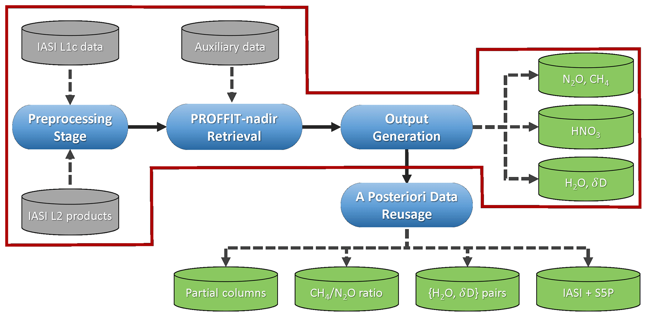
Figure 1Outline of the MUSICA IASI processing chain. This paper focuses on the processing steps as indicated by the red frame. The green symbols indicate different products. The supply of detailed information on retrieval settings and product characteristics offers many different possibilities for a posteriori processing and date reusage as indicated at the bottom of the schematics and discussed in Sect. 8 (S5P here means the main sensor on the Sentinel-5 Precursor satellite).
The paper is organised as follows: Sect. 2 briefly presents the satellite experiment on which the retrieval product relies. Section 3 describes the structure of the data files, the data volume, and the nomenclature of the data variables. In Sect. 4 we discuss the details of the MUSICA IASI retrieval setup. There we describe the cloud filtering and the comprehensive information that is provided about the a priori state vectors and the generation of the applied constraints. This information is essential for being able to perform a posteriori processing according to Diekmann et al. (2021) or to optimally combine the data with other remote sensing data products (e.g. Schneider et al., 2021c). Section 4 can be skipped by readers that do not plan such complex data reuse. In Sect. 5 the data variables and the variables describing the quality of the data are explained. This is of general importance for correctly using the data (understanding uncertainties, representativeness, application in the context of model comparisons and data assimilation systems, application for inter-comparison studies, etc.). In Sect. 6 the options for filtering data according to their quality and characteristics are discussed. This enables the user to develop their own tailored data filtering. Section 7 visualises the data volume in the form of two examples. A first example shows the continuous data availability over several years and a second example the good global daily data coverage. Section 8 discusses the potential of the data set in regard to data interoperability and data reuse, which is achieved by providing the retrieved state vectors together with comprehensive information on the a priori state vectors, the constraint matrices, the averaging kernels matrices, and the error covariance matrices. A summary and an outlook are provided in Sect. 10. For readers that are no experts in the field of remote sensing retrievals, Appendix A provides a short compilation with the theoretical basics and the most important equations to which we refer throughout this paper. Appendix B reveals that for the MUSICA IASI retrieval product we can assume moderate non-linearity (according to chap. 5 of Rodgers, 2000), which is important for many data reuse options. Appendix C explains how the data can be used in the form of a total or partial column product.
IASI is a Fourier-transform spectrometer and measures in the infrared part of the electromagnetic spectrum between 645 and 2760 cm−1 (15.5 and 3.63 µm). After apodisation (L1c spectra) the spectral resolution is 0.5 cm−1 (full width at half maximum, FWHM). The main purpose of IASI is the support of numerical weather prediction. However, due to its high signal-to-noise ratio and the high spectral resolution, the IASI measurements offer very interesting possibilities for atmospheric trace gas observations (e.g. Clerbaux et al., 2009).
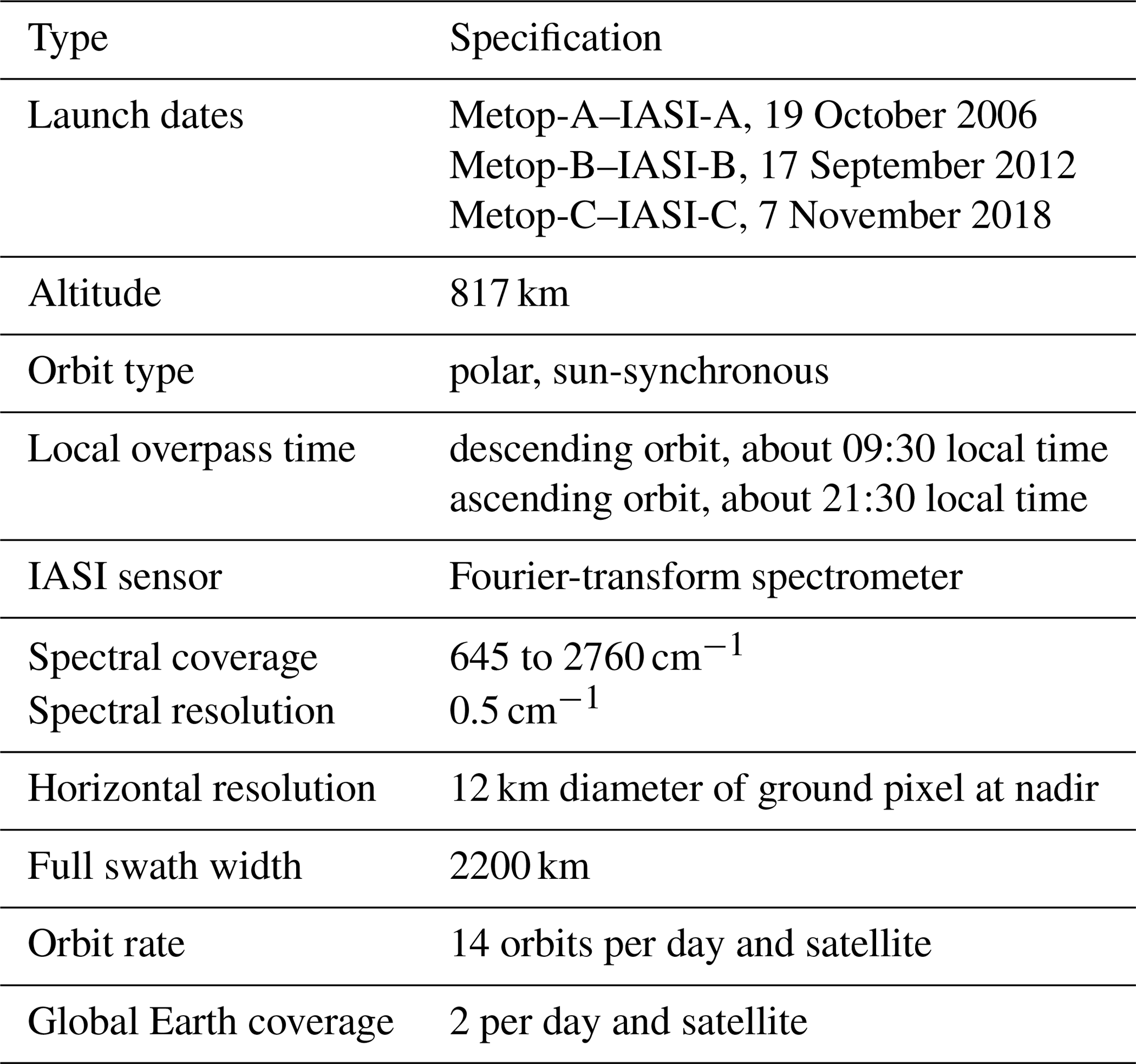
The IASI instruments are carried by the Metop satellites, which are Europe's first polar-orbiting satellites dedicated to operational meteorology. The Metop programme has been planned as a series of three satellites to be launched sequentially over an observational period of 14 years. Metop-A was launched on 19 October 2006, Metop-B on 17 September 2012, and Metop-C on 7 November 2018. IASI is the main payload instrument and operates in the nadir viewing geometry with a horizontal resolution of 12 km (pixel diameter at nadir viewing geometry) over a swath width of about 2200 km. With 14 orbits in a sun-synchronous mid-morning orbit (09:30 local solar time, LT, descending node), each IASI on a Metop satellite provides observations twice a day at middle and low latitudes (at about 09:30 and 21:30 LT) and several times a day at high latitudes. Metop-A, Metop-B, and Metop-C overflight times generally take place within about 45 min. Table 1 gives an overview of the major specifications of the Metop–IASI mission.
The number of individual observations made by the three currently orbiting IASI instruments is tremendous. During a single orbit 91 800 observations are made. In 24 h the three satellites conclude in total about 42 orbits, which means more than 3.85 million individual IASI spectra per day and more than 1.4 billion per year.
IASI-like observations are guaranteed for several decades. The first observations were made in 2006. In the context of the Metop – Second Generation (Metop-SG) satellite programme, IASI–Next Generation (IASI-NG) instruments will perform measurements until the 2040s. In this context the IASI programme offers unique possibilities for studying the long-term evolution of the atmospheric composition.
In this section we discuss the format of the MUSICA IASI full product data files and the nomenclature of the data variables.
3.1 Data files
The MUSICA IASI full product data are provided as netCDF files compliant with version 1.7 of the CF (Climate and Forecast) metadata convention (https://cfconventions.org, last access: 25 January 2022). The data files contain all information needed for reproducing the retrievals and for optimally reusing the data. Because the MUSICA IASI retrieval builds upon the EUMETSAT L2 cloud filter and uses the EUMETSAT L2 atmospheric temperature as the a priori atmospheric temperature, the output files contain some EUMETSAT retrieval data as well as the MUSICA retrieval data. In addition, they contain the EUMETSAT L1C spectral radiances (and the simulated radiances) as well as auxiliary data needed for the retrieval (like surface emissivity from other sources; Masuda et al., 1988; Seemann et al., 2008; Baldridge et al., 2009).
We provide standard output files comprising all processed IASI observations and one extended output file with detailed calculations of Jacobians (and spectral responses for surface emissivity, spectroscopic parameters, and cloud coverage) and gain matrices for a few selected observations.
The standard output is provided in the files “IASI[S]_MUSICA_[V]_L2_AllTargetProducts_[D]_[O].nc” and in one file per orbit and instrument. The symbols within the square brackets indicate placeholders: “[S]” for the sensor (A, B, or C, for IASI instruments on the satellites Metop-A, Metop-B, or Metop-C, respectively), “[V]” for the MUSICA IASI retrieval processor version used, “[D]” for the starting date and time of the observation (format YYYYMMDDhhmmss), and “[O]” for the number of the orbit.
In our database these files are provided in daily .tar files, with all orbits of all IASI instruments archived into a single .tar file, with the name “IASI[multipleS]_MUSICA_[V]_L2_AllTargetProducts_[DAY].tar”. The placeholders are as follows: “[multipleS]” for the considered sensors, e.g. AB if IASI sensors on Metop-A and Metop-B are considered; “[V]” for the MUSICA IASI retrieval processor version used; and “[DAY]” for the date of observations (universal time, format YYYYMMDD). The typical size of a .tar file with the orbit-wise netCDF files of a single day is 15 GB. This number is for the typically 28 orbits per day of two satellites (for three satellites there are typically 42 orbits per day). The standard output data files are linked to a DOI (Schneider et al., 2021b).
The extended file represents 74 observations over polar, mid-latitudinal, and tropical GRUAN stations (GRUAN stands for Global Climate Observing System Reference Upper-Air Network, https://www.gruan.org, last access: 25 January 2022). More details on the time periods and locations represented by these retrievals are given in Borger et al. (2018). The file provides the same output as the standard files and in addition detailed information on Jacobians (and spectral responses) and gain matrices. The Jacobian matrices collect the derivatives of the radiances as measured by the satellite sensors with respect to a parameter (e.g. atmospheric temperature, instrumental conditions). The spectral response matrices give information about the change in the radiances due to changes in the surface emissivities, the spectroscopic parameters, and the cloud coverage. The gain matrices are the derivatives of the retrieved atmospheric state with respect to the radiances. The name of this extended output file is “IASIAB_MUSICA_030201_L2_AllTargetProductsExtended_examples.nc”; its size is 70 MB, and it is linked to an extra DOI (Schneider et al., 2021a).
Here we report on the MUSICA IASI processing version 3.2.1 (applied for IASI observations until the end of June 2019). For observations from July 2019 onward processing versions 3.3.0 and 3.3.1 are applied (the difference of version 3.3.1 with respect to 3.3.0 is updated a priori data for the retrievals of observations from January 2021 onward). Version 3.2.1 and the versions 3.3.x use the same retrieval setting, and the output files contain the same variables. The difference between version 3.2.1 and the versions 3.3.x is that for the former some minor corrections were necessary after the retrieval process due to some very minor inconsistencies in version 3.2.1 with regard to the following: the vertical gridding; the a priori of δD; and the constraint for N2O, CH4, and HNO3. This difference between the versions is actually not noticeable by the user, and the report provided here on version 3.2.1 data is also valid for data of versions 3.3.x, which will soon be made available for the public in the same format as the version 3.2.1 data.
3.2 Variables
There are three different categories of variables. The first category consists of variables that contain information resulting from the EUMETSAT L2 PPF (product processing facility) retrieval. They can be identified by the prefix eumetsat_ in their names. A second category consists of variables that contain information from the MUSICA IASI retrieval. Here the prefix in the name is musica_. The third category encompasses all other variables, and their names have no specific prefix.
The EUMETSAT L2 retrieval variables are flags (mainly for cloud coverage – see Sect. 4.1, surface conditions, and EUMETSAT retrieval quality) and the EUMETSAT L2 retrieval output of H2O. The variables belonging to the third category are supporting data and inform about the sensors' viewing geometry, observation time, measured radiances, climatological tropopause altitude, and surface emissivity. Although our MUSICA IASI retrieval uses the EUMETSAT L2 PPF version 6 land surface emissivity, the emissivity variables are assigned to the category of supporting data, because for older observations where no L2 PPF version 6 is available we use the surface emissivity climatology from IREMIS (Seemann et al., 2008) and over water we always use the values reported by Masuda et al. (1988). The large majority of variables are MUSICA IASI variables. These variables document the MUSICA IASI retrieval settings (like the a priori states and constraints; see Sect. 4.4 to 4.6), provide the MUSICA IASI retrieval products (retrieved trace gas profiles, Sect. 5.1), and characterise these products (averaging kernels, estimated errors, Sect. 5.2). For variables that refer to a specific retrieval product, a corresponding syllable is embedded into the respective variable names: _wv_ and _wvp_ stand for water vapour isotopologues and water vapour isotopologue proxies, respectively; _ghg_ for the greenhouse gases N2O and CH4, _hno3_ for HNO3; and _at_ for the atmospheric temperature.
The water vapour and greenhouse gas variables (_wv_, _wvp_, and _ghg_) contain information on two species, which can be identified by the value of the dimension musica_species_id. For _wv_ these are the species H2O and HDO, for _wvp_ the water vapour proxy species (see Sect. 4.4.2), and for _ghg_ the species N2O and CH4.
In this section the principle setup of the MUSICA IASI retrieval is presented. We discuss our filtering before processing, the retrieval algorithm used, the measurement state (spectral region), the atmospheric state that is retrieved in an optimal estimation sense, and the a priori information used and the applied constraints. A detailed explanation of these settings ensures the full reproducibility of the data and is also important in the context of data reusage (see examples given in Sect. 8).
4.1 Data selection prior to processing
We focus on the processing of IASI data for which EUMETSAT L2 data files of PPF version 6.0 or later are available. For former data versions not all of the subsequently discussed L2 PPF variables are available. Furthermore, we found that there are several modifications made within versions 4 and 5 that significantly affect the stability of our MUSICA IASI retrieval output (see discussion in García et al., 2018). EUMETSAT L2 PPF version 6 data are available from October 2014 onward, so we focus our processing on IASI observations made from October 2014 onward.
In addition, the MUSICA IASI retrievals are currently restricted to cloud-free scenarios. The selection of cloud-free conditions is made by means of the EUMETSAT L2 PPF cloudiness assessment summary flag variable (called flag_cldnes in the EUMETSAT L2 netCDF data files). We only process IASI observations with this flag having the value 1 (the IASI instrumental field of view, IFOV, is clear) or 2 (the IASI IFOV is processed as cloud-free, but small cloud contamination is possible). This requirement for cloud-free scenarios removes more than two-thirds of all available IASI observations.
Furthermore, we require EUMETSAT L2 PPF temperature profiles to be generated by the EUMETSAT L2 PPF optimal estimation retrieval scheme. For this purpose we use the EUMETSAT L2 PPF variable flag_itconv. We only process data with this flag having value 3 (the minimisation did not converge, sounding accepted) or 5 (the minimisation converged, sounding accepted).
Figure 2 gives a climatological overview of the number of IASI data that remain after the aforementioned preselection. The maps largely reflect the cloud cover conditions. A very large number of IASI data passed our selection criteria in the subtropical regions, where cloud-free conditions generally prevail. In the North Atlantic storm track region, the southern American and southern African tropics, and the southern polar oceans the sky is generally cloudy in February, leading to a low number of IASI observations that passed our selection criteria. In August we can clearly identify the Asian and West African monsoon region as an area with increased cloud coverage and consequently fewer MUSICA IASI processed data.
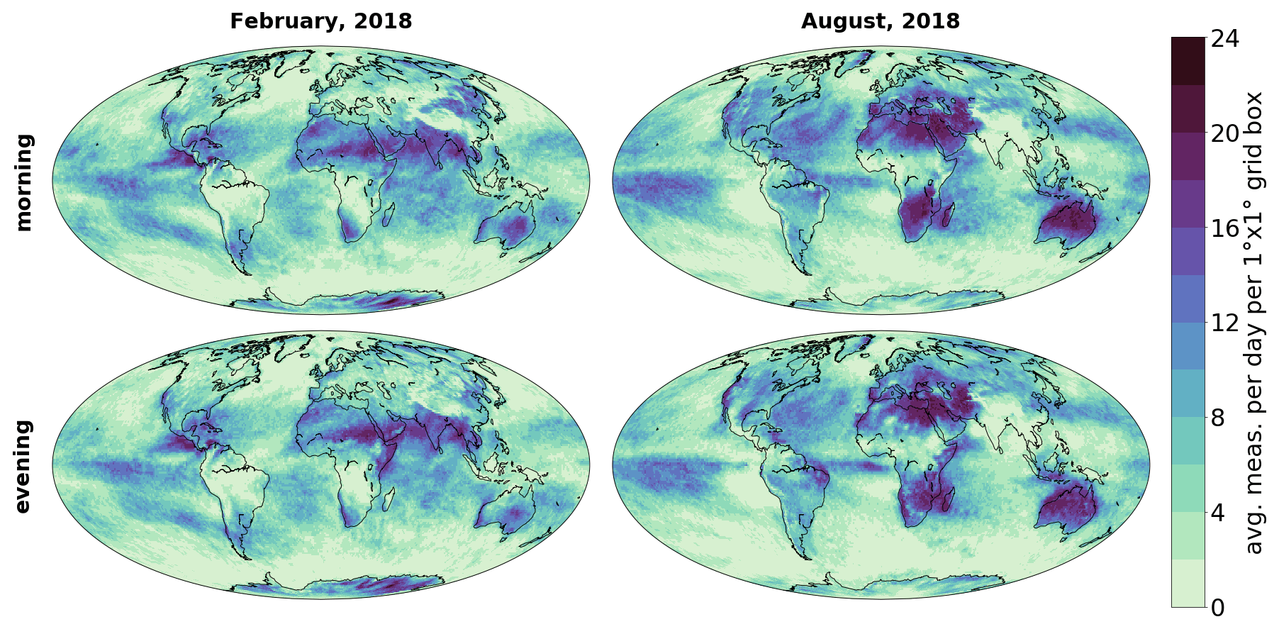
Figure 2Monthly averaged number of the IASI observations per box that passed our selection criteria prior to the MUSICA IASI processing, for February and August 2018 and for local morning and evening overpasses.
Figure 3 is similar to Fig. 2, but instead of showing the total number of observations that fall within a box, it depicts the probability of having at least one observation per overpass in a box. In both figures we observe very similar structures.
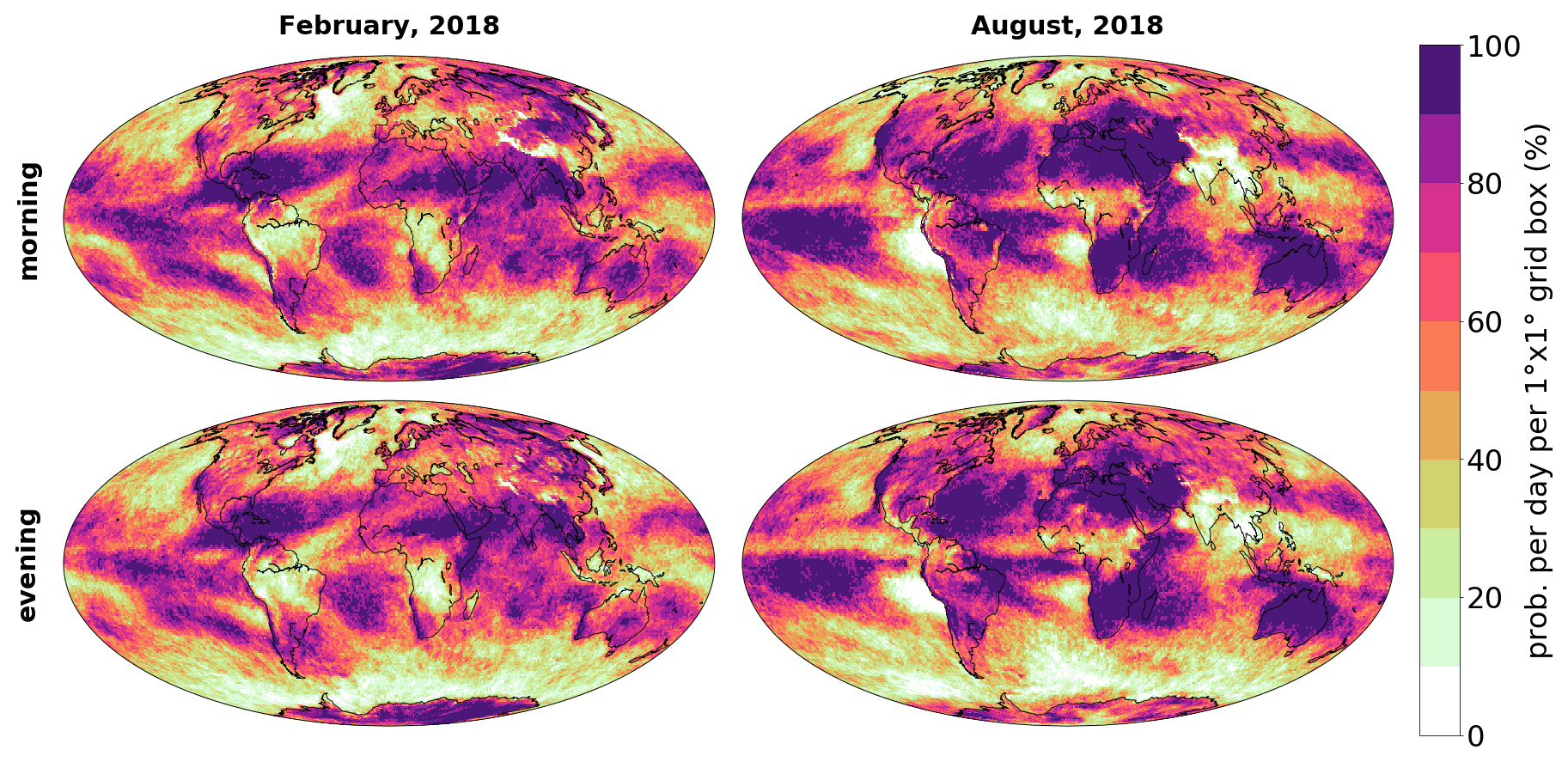
Figure 3Similar to Fig. 2 but for the probability of having at least one valid IASI observation (measurement that passed the cloud filter and EUMETSAT quality checks) per overpass and box.
4.2 The retrieval algorithm
We use the thermal nadir retrieval algorithm PROFFIT-nadir (Schneider and Hase, 2011; Wiegele et al., 2014). It is an extension of the PROFFIT algorithm (PROFile FIT; Hase et al., 2004) that has been used for many years by the ground-based infrared remote sensing community (Kohlhepp et al., 2012; Schneider et al., 2012). This extension has been made in support of the IASI retrieval development during the project MUSICA. The algorithm consists of the line-by-line radiative transfer code PROFFWD (Hase et al., 2004; Schneider and Hase, 2009) and can consider Voigt as well as non-Voigt line shapes (Gamache et al., 2014) and the water continuum signatures according to the model MT_CKD v2.5.2 (Delamere et al., 2010; Payne et al., 2011; Mlawer et al., 2012). For the MUSICA IASI processing we use the water continuum model MT_CKD v2.5.2 and for all trace gases a Voigt line shape model and the spectroscopic line parameters according to the HITRAN2016 molecular spectroscopic database (Gordon et al., 2017). However, we increase the line intensity parameter for all HDO lines by +10 % in order to correct for the bias observed between MUSICA IASI δD retrievals and respective aircraft-based in situ profile data (Schneider et al., 2015).
For the inversion calculations PROFFIT-nadir offers options that are essential for water vapour isotopologue retrievals. These are the options for logarithmic-scale retrievals and for setting up a cross constraint between different atmospheric species (see also Sect. 4.4.2). The theoretical basics for atmospheric trace gas retrievals are provided in Appendix A.
4.3 The analysed spectral region
The retrieval works with the radiances measured in the spectral region between 1190 and 1400 cm−1. The respective radiance values are the elements of the MUSICA IASI measurement state vector referred to as y in Appendix A. Figure 4 depicts measured and simulated radiances as well as a large variety of different spectral responses (Jacobians multiplied by parameter changes) for a typical mid-latitudinal summer observation over land. Please note the different radiance scales for measurement and simulation, on the one hand, and residuals and spectral responses, on the other hand.
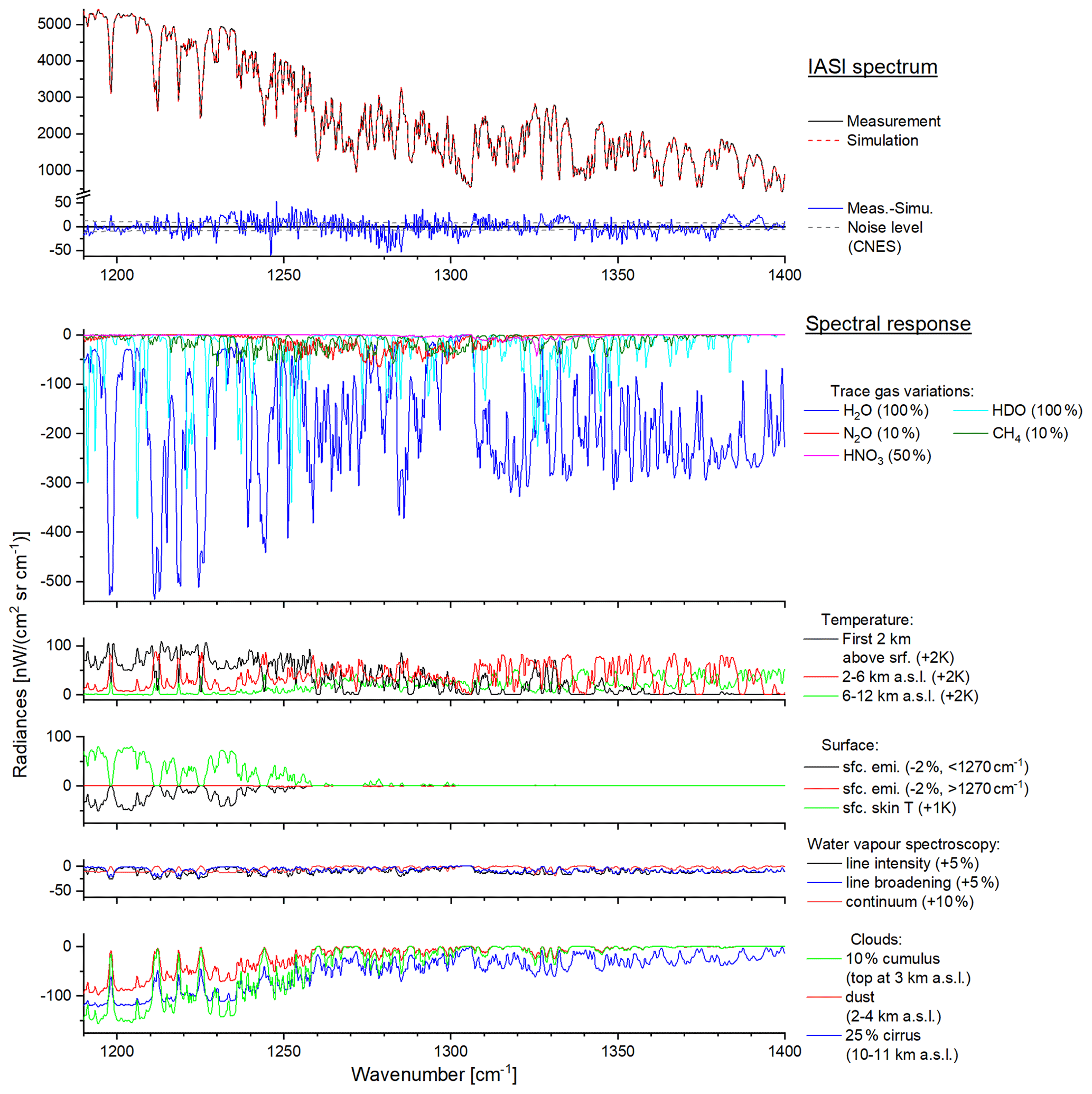
Figure 4Example for a spectrum, residual (difference between the measured and simulated spectrum) and different spectral responses (Jacobians multiplied by parameter change) for an observation over the mid-latitudinal site of Lindenberg on 30 August 2008 (satellite nadir angle: 43.7∘; surface skin temperature: 292.3 K; precipitable water vapour: 31.8 mm).
We show trace gas spectral responses for a uniform increase in the trace gases throughout the whole atmosphere: 100 % for H2O and HDO, 10 % for N2O and CH4, and 50 % for HNO3. The respective values are reasonable approximations of the typical atmospheric variabilities of these trace gases. We see that the measured radiances are most strongly affected by the water isotopologues. The variations in N2O and CH4 are also recognisable (larger than the spectral residuals, i.e. the difference between measured and simulated radiances). The spectral responses of HNO3 are very close to the noise level.
The atmospheric temperature spectral responses are depicted for a uniform 2 K temperature increase over three different layers: surface–2, 2–6, and 6–12 km a.s.l. (a.s.l. means above sea level). In the analysed spectral region (1190–1400 cm−1), the atmospheric temperature variations close to the surface affect mainly the radiances below 1300 cm−1 and variations at higher altitudes mainly the radiances above 1300 cm−1. In Fig. 4 we depict the spectral responses for 2 K because this is a reasonable approximation of the uncertainty in the EUMETSAT L2 PPF temperatures (August et al., 2012).
The spectral responses for surface emissivity and temperature reveal that surface properties hardly affect the radiances above 1250 cm−1 but have a strong impact below 1250 cm−1. We calculate the emissivity spectral responses for a −2 % change in the emissivity independently above and below 1270 −1, which is a typical uncertainty in emissivity judging from its dependency on the viewing angle and wind speed over ocean (Masuda et al., 1988) and small-scale inhomogeneities; however, this uncertainty might be significantly higher over arid areas (Seemann et al., 2008).
Concerning spectroscopy, the spectral responses calculated for the typical uncertainty range of spectroscopic parameters are relatively small. In Fig. 4 we show the spectral responses for consistent +5 % changes in the line intensity and pressure-broadening parameters of all water vapour isotopologues, which are in reasonable agreement with the uncertainty values given by HITRAN (Gordon et al., 2017). Concerning the water continuum, the spectral responses are for a water continuum that is 10 % larger than the continuum according to the model MT_CKD v2.5.2 (Delamere et al., 2010; Payne et al., 2011; Mlawer et al., 2012).
The bottom panel of Fig. 4 depicts the impact of clouds on the radiances. The thermal nadir radiance when observing over an opaque cloud can be calculated by defining the cloud top instead of the surface as the thermal background. Cirrus and mineral dust clouds are not opaque, and we have to consider partial attenuation by the cloud particles. We calculate the attenuated radiances using forward model calculations from KOPRA (Karlsruhe Optimized and Precise Radiative transfer Algorithm; Stiller, 2000) and consider single scattering. The frequency dependency of the extinction cross sections, the single-scattering albedo, and the scattering phase functions of the clouds are calculated from OPAC v4.0b (Optical Properties of Aerosol and Clouds; Hess et al., 1998; Koepke et al., 2015). For cirrus clouds we assume the particle composition as given by OPAC's “Cirrus 3” ice cloud example (see Table 1b in Hess et al., 1998) and for mineral dust clouds a particle composition according to OPAC's “Desert” aerosol composition example (see Table 4 in Hess et al., 1998). The spectral responses shown are for 10 % cumulus cloud coverage with the cloud top at 3 km, a homogeneous dust cloud between 2 and 4 km, and 25 % cirrus cloud coverage between 10 and 11 km. These are relatively weak clouds, and we assume that they might occasionally not correctly be identified by the EUMETSAT L2 cloud screening algorithm. Because the respective spectral responses are significantly above the noise level, these unrecognised clouds can have an important impact on the retrieval.
A comprehensive set of different spectral responses is provided with the extended output data file for the 74 exemplary observations at an Arctic, mid-latitudinal, and tropical site.
4.4 The state vector
In this section we discuss the MUSICA IASI state vector, which is referred to as x in Appendix A.
4.4.1 Components of the state vector
We retrieve vertical profiles of the trace gases H2O, HDO, N2O, CH4, and HNO3 and of atmospheric temperature. For all these profile retrievals we use constraints (for more details see Sect. 4.6). In addition we fit the surface skin temperature and the spectral frequency scale without any constraint. We discretise the profiles on atmospheric levels between the surface and the top of the atmosphere (which we set at 56 km). The grid is relatively fine in the lower troposphere (≈400 m) and increases in the stratosphere to above 5 km. The number of atmospheric levels (nal) depends on the surface altitude. For instance, for a surface altitude at sea level (0 m a.s.l.) nal=28 and for a surface altitude of 4000 m a.s.l. nal=21. Consequently, the state vector for an observation with surface altitude at sea level has a length of .
4.4.2 Water vapour isotopologue proxies
The water vapour isotopologues H2O and HDO vary largely in parallel. The information that HDO actually adds to H2O lies in the value of the ratio. This ratio is typically expressed as , with VSMOW being (VSMOW – Vienna Standard Mean Ocean Water). In Schneider et al. (2006b) the logarithmic-scale difference between H2O and HDO was introduced as a good proxy for δD, and Schneider et al. (2012) showed that by a transformation between the state {H2O,HDO} – needed for the radiative transfer calculations – and the proxy state {,} – where we can formulate the correct constraints – the climatologically expected variability in the atmospheric state can be described correctly.
First we have to transfer the associated mixing ratio entries in the state vector to a logarithmic scale. This means that all the derivatives provided by the radiative transfer calculations have to be transferred from the linear scale to the logarithmic scale by using . For highly variable trace gases logarithmic-scale retrievals are advantageous because they allow the consideration of the correct a priori statistics (log-normal instead of normal distributions; Hase et al., 2004; Schneider et al., 2006a). For trace gases with weak variability but still detectable spectral signatures, the statistics in logarithmic and linear scale become very similar, so logarithmic-scale retrievals have no apparent disadvantage with respect to linear-scale retrievals; instead they offer unique possibilities as outlined in the following. In the logarithmic scale the water vapour isotopologue state can be expressed in the basis of {ln [H2O],ln [HDO]} or in the basis of the proxy state . Both expressions are equally valid. Each basis has the dimension (2×nal). In the following the full water vapour isotopologue state vector expressed in the {ln [H2O],ln [HDO]} basis and the proxy basis will be referred to as x and x′, respectively. The basis transformation can be achieved by operator P:
Here the four matrix blocks have the dimension (nal×nal), I stands for an identity matrix, and the state vectors x and x′ are related by
Similarly logarithmic-scale covariance matrices can be expressed in the two basis systems, and the respective matrices S and S′ are related by
and respective averaging kernel matrices A and A′ are related by
In contrast to H2O and HDO, H2O and δD vary to a large extent independently, and we can easily set up the constraint matrix R′ for the proxy basis :
Back transformation to the {ln [H2O],ln [HDO]} basis reveals automatically the strong cross constraints between H2O and HDO:
For more details on the utility of the water vapour isotopologue proxy state please refer to Schneider et al. (2012) and Barthlott et al. (2017).
4.4.3 Summary
The atmospheric state variables that are independently constrained during the MUSICA IASI processing are the vertical profiles of the water vapour isotopologue proxies H2O and δD and the vertical profiles of N2O, CH4, HNO3, and atmospheric temperature. For all the trace gases (not only for the water vapour isotopologues) the retrieval works with the state variables in a logarithmic scale. For atmospheric temperature a linear scale is used. Surface skin temperature and the spectral frequency shift are also components of the state vector; however, they are not constrained during the retrieval procedure. The reason for this is that surface skin temperature and spectral frequency shift can be identified very clearly in the spectra. There is no need to impose a priori information and thereby constrain these retrieved quantities. Also without such constraint the retrieval converges in a very stable manner.
The variables musica_wv_apriori and musica_wv provide the a priori assumed and the retrieved values of H2O and HDO, respectively (see also Sects. 4.5 and 5.1). The output is given in parts per million as a volume fraction (ppmv) and normalised with respect to the naturally occurring isotopologue abundance. In this context, δD is calculated from the content of these variables as . Information about H2O and δD related to differentials (constraints, averaging kernels, kernel metrics, or uncertainties) is generally provided in the proxy states (variables with the term _wvp_).
4.5 A priori states
The reference for the a priori data used for the MUSICA IASI trace gas retrievals is the CESM1–WACCM (Community Earth System Model version 1 – Whole Atmosphere Community Climate Model) monthly output of the 1979–2014 time period. The CESM1–WACCM is a coupled chemistry climate model from the Earth's surface to the lower thermosphere (Marsh et al., 2013). The horizontal resolution is 1.9∘ latitude × 2.5∘ longitude. The vertical resolution in the lower stratosphere ranges from 1.2 km near the tropopause to about 2 km near the stratopause; in the mesosphere and thermosphere the vertical resolution is about 3 km. Simulations used for generating the MUSICA IASI a priori data are based on the International Global Atmospheric Chemistry–Stratosphere-troposphere Processes And their Role in Climate (IGAC–SPARC) Chemistry Climate Model Initiative (CCMI; Morgenstern et al., 2017). From the surface to 50 km the meteorological fields are “nudged” towards meteorological analysis taken from the National Aeronautics and Space Administration (NASA) Global Modeling and Assimilation Office (GMAO) Modern-Era Retrospective Analysis for Research and Applications (MERRA; Rienecker et al., 2011), and above 60 km the model meteorological fields are fully interactive, with a linear transition in between (details about the nudging approach are described in Kunz et al., 2011).
For the MUSICA IASI a priori profiles of H2O, N2O, CH4, and HNO3, we consider a mean latitudinal dependence, seasonal cycles, and long-term evolution. Therefore, the a priori data are constructed by means of a low dimensional multi-regression fit on the CESM1–WACCM data independently for each vertical grid level. We fit an annual cycle with the two frequencies 1 per year and 2 per year, and for the long-term baseline we fit a second-order polynomial. The fits are performed individually for 15 equidistant latitudinal bands between 90∘ S and 90∘ N. In order to capture the yearly anomalies in N2O and CH4 a priori data, we use the Mauna Loa Global Atmospheric Watch yearly mean data records for a correction of the WACCM parameterised time series (for more details on this correction procedure see Barthlott et al., 2015). We also use the temperature lapse rate tropopause – according to the definition of the World Meteorological Organization – from WACCM and construct a latitudinally dependent tropopause altitude by fitting a seasonal cycle and a constant baseline (no long-term dependency) and assume a transition zone between the troposphere and stratosphere with a vertical extension of 12.5 km. The MUSICA IASI δD a priori profiles between the ground and the tropopause altitude are constructed from the H2O a priori profiles by using a single global relation between tropospheric H2O concentration and δD values. This relation has been determined from simultaneous H2O and δD measurements made by high-precision in situ instruments at different ground stations located in the mid-latitudes and the subtropics and between 100 m and 3650 m a.s.l. (González et al., 2016; Christner et al., 2018) and by aircraft-based in situ measurements made between the sea surface and about 7000 m a.s.l. (Dyroff et al., 2015). Above the troposphere (where δD is close to −600 ‰) we smoothly connect the tropospheric δD values with the typical stratospheric δD value of −350 ‰.
Figure 5 depicts the MUSICA IASI a priori data derived from WACCM. It shows latitudinal cross sections for a northern hemispheric winter and summer day as well as the temporal evolution between 2014 and 2020 at a mid-latitudinal site. The H2O and δD a priori data have strong latitudinal gradients and also a marked seasonal cycle. For δD the lowest values are in the neighbourhood of the tropopause altitude (depicted as a thick violet line). The a priori values of N2O and CH4 have a strong latitudinal and seasonal variability in the tropopause region. CH4 has a strong tropospheric latitudinal gradient and seasonal cycle in the troposphere, whereas the tropospheric N2O variability is rather small. The HNO3 a priori has a maximum in the lower stratosphere (20–25 km) with the highest values at higher latitudes.
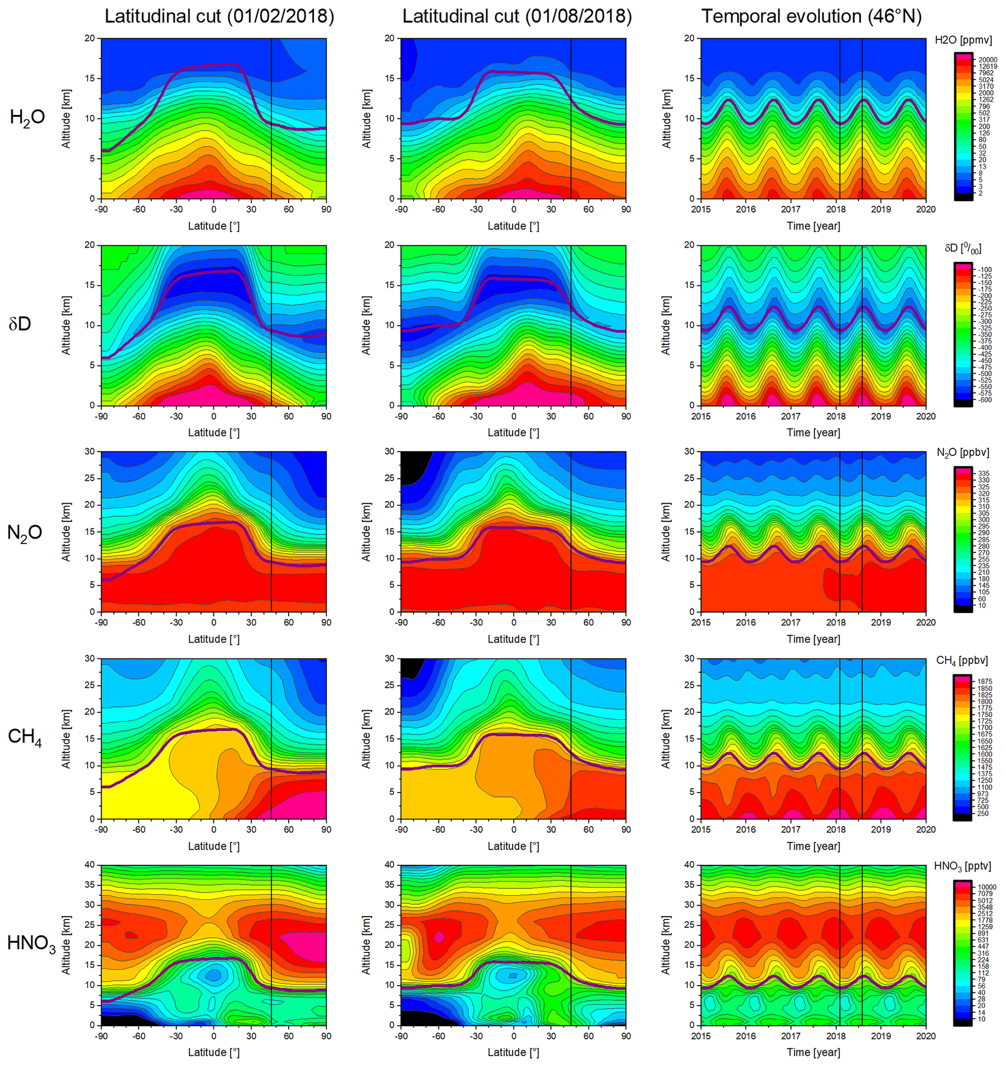
Figure 5Overview of time- and latitude-dependent a priori information (source – WACCM model simulations) used for the MUSICA IASI retrieval for all targeted atmospheric species (H2O, δD, N2O, CH4, and HNO3) and for the tropopause altitude (depicted as thick solid violet line). Shown are latitudinal cross sections for 1 February 2018 and 1 August 2018 and the temporal evolution at 46∘ N for the 2015–2020 time period. Please note the non-uniform y-axes scales.
The a priori trace gas profiles are provided in the variables musica_wv_apriori (H2O and HDO with species index 1 and 2, respectively), musica_ghg_apriori (N2O and CH4 with species index 1 and 2, respectively), and musica_hno3_apriori (HNO3). The unit is ppmv.
As a priori for the atmospheric and the surface temperatures we use the EUMETSAT L2 PPF atmospheric temperature output. These data are provided in the unit kelvin and in the variables musica_at_apriori and musica_st_apriori for atmospheric temperature and surface temperature, respectively.
4.6 A priori covariances and constraints
We set up simplified a priori covariance matrices by means of two parameters. The first parameter is the altitude-dependent amplitudes of the variability (vamp,i, with i indexing the ith altitude level). For the trace gases we work with the relative variability, i.e. with the variability on the logarithmic scale. For atmospheric temperatures the variability is given in the unit kelvin. The second parameter is the altitude-dependent vertical correlation lengths (σcl,i, for considering correlated variations between different altitudes). The elements of the a priori covariance matrix (Sa) are then calculated as
with zi being the altitude at the ith altitude level.
The values vamp,i and σcl,i are oriented to the typical covariances of in situ observations made from the ground (e.g. González et al., 2016; Gomez-Pelaez et al., 2019), aircraft (e.g. Wofsy, 2011; Dyroff et al., 2015), or balloons (e.g. Karion et al., 2010; Dirksen et al., 2014) and also aligned to the vertical dependency of the monthly mean covariances we obtain from the WACCM simulations. For the vamp,i of δD we use in addition the isotopologue-enabled version of the Laboratoire de Météorologie Dynamique (LMD) general circulation model as a reference (Risi et al., 2010; Lacour et al., 2012). For atmospheric temperature we use the uncertainty in the EUMETSAT L2 atmospheric temperature as reference (August et al., 2012). Generally, we classify three different altitude regions with specific vertical dependencies in the values of vamp,i and σcl,i: the troposphere (below the climatological tropopause altitude as depicted in Fig. 5), the stratosphere (starting 12.5 km above the climatological tropopause altitude), and the transition region between the troposphere and stratosphere.
The values of vamp,i are specific for each trace gas and for the atmospheric temperature, and they are provided in the MUSICA IASI standard output files in the variables having the suffix _apriori_amp.
As a simplification we use the same values of σcl,i for all trace gases and for the atmospheric temperature. These values are provided in the MUSICA IASI output files as the variable musica_apriori_cl.
As the constraint of the retrieval we use an approximation of the inverse of the covariance matrix. For this purpose the constraint matrix R is constructed as a sum of a diagonal constraint, and first- and second-order Tikhonov-type regularisation matrices (Tikhonov, 1963):
with
and
The diagonal elements of the diagonal matrices α0, α1, and α2 are the inverse of the absolute variabilities and the variabilities of the first and the second vertical derivatives of the profiles. These values can be calculated from the elements of the a priori matrix (Sa) as follows:
Starting the retrievals with the constraint matrix optimises the computational efficiency of the retrieval processes because according to Eqs. (A4) and (A5) the retrieval calculations work with . Furthermore, calculating the inversion of Sa approximatively as the sum of diagonal constraint and first- and second-order Tikhonov-type regularisation matrices offers the possibility of tuning the constraint according to specific user requirements with respect to smoothness or absolute deviations (e.g. Steck, 2002; Diekmann et al., 2021).
For the greenhouse gases (N2O and CH4) and HNO3 we constrain with respect to the absolute values of the profiles and the first derivative of the profile; i.e. we do not consider the term (α2L2)Tα2L2 of Eq. (8). In the case of the water vapour isotopologue proxies and the atmospheric temperature, we additionally constrain with respect to the second derivative of the profile; i.e. we consider all terms of Eq. (8). Please note that for the trace gases the constraints work on the logarithmic scale and for the atmospheric temperature on the linear scale.
Because HNO3 has only very weak spectroscopic signatures in the analysed spectral region (see Fig. 4), we loosen the absolute constraint and at the same time strengthen the constraint with respect to the first vertical derivate: α0 and α1 are calculated from an Sa constructed with the values of vamp,i increased by a factor of 1.5 and with the values of σcl,i increased by a factor of 2. Similarly and in order to avoid a negative impact of an underconstrained retrieval of the temperature profile on the trace gas products (e.g. artificial oscillatory features), we strengthen the atmospheric temperature constraint: α0, α1, and α2 are calculated from an Sa constructed with the values of vamp,i decreased by a factor of 0.5.
The diagonal entries of the diagonal matrices α0, α1, and α2 contain all information about the actual constraints used by the retrieval. They are provided in the MUSICA output files for each individual retrieval and for the different trace gases and the atmospheric temperature as variables with the suffix _reg. For the trace gases these vector elements are depicted in Fig. 6 for a northern hemispheric summer in the tropics, mid-latitudes, and polar regions. The dotted lines indicate the climatological tropopause and the altitude 12.5 km above this tropopause (transition zone between the troposphere and stratosphere).
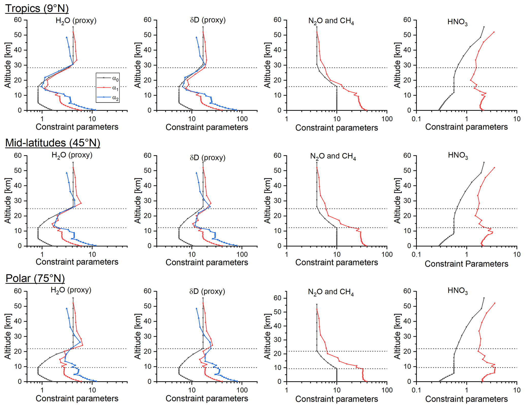
Figure 6Vertical profiles of the constraint parameter (diagonal elements of the diagonal matrices α0, α1, and α2) for the retrieval of all targeted atmospheric species (H2O, δD, N2O, CH4, and HNO3). The parameters are latitudinal and time dependent. Shown are examples for 8 July 2018 for the tropics (9∘ N), mid-latitudes (45∘), and polar regions (75∘). The area between the dotted lines indicates the transition between the troposphere and stratosphere.
In this sections we describe the variables that give information about the retrieval target products (vertical trace gas profiles) and the characteristics of these products (averaging kernels and errors). A detailed explanation of these data supports their interoperability and is also important in the context of data reusage (see examples given in Sect. 8).
5.1 Trace gas profiles and temperatures
The retrieved trace gas profiles are provided in the variables musica_wv (H2O and HDO with species index 1 and 2, respectively), musica_ghg (N2O and CH4 with species index 1 and 2, respectively), and musica_hno3 (HNO3). The unit is ppmv. The retrieved atmospheric temperature is provided in the variable musica_at and the retrieved surface temperature in the variable musica_st. The unit is kelvin.
In order to provide a brief insight into the data diversity, Fig. 7 gives examples with a priori and retrieved trace gas profiles for an observation on 30 August 2008 over Lindenberg (53∘ N). The profile data represent 28 altitude levels and are provided with detailed information on their sensitivity, vertical representativeness, and errors (see following subsections).
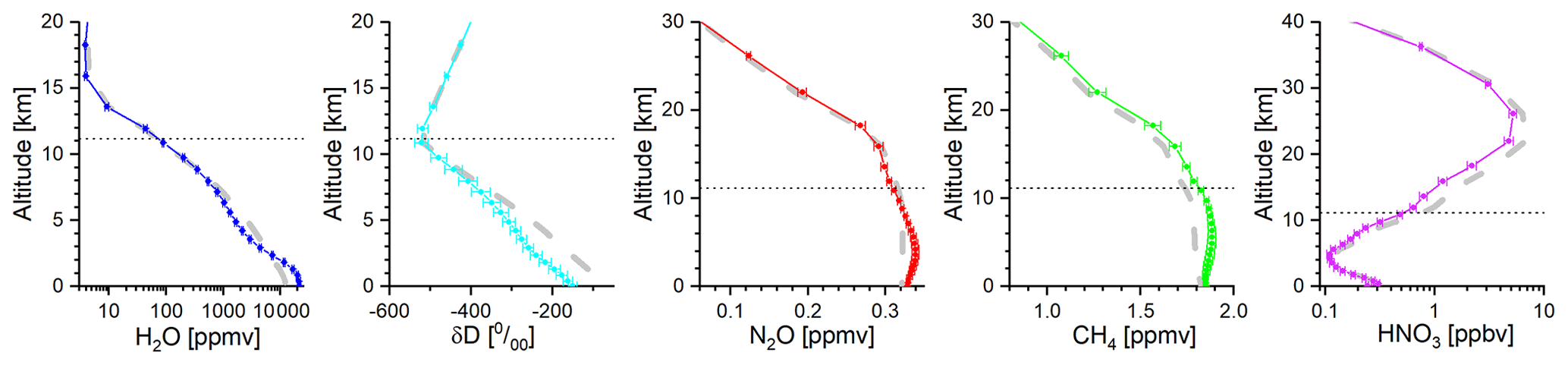
Figure 7Example of vertical profiles of the targeted atmospheric trace gas products (H2O, δD, N2O, CH4, and HNO3): thick grey dashed lines represent the a priori assumption, and the coloured line with symbols and error bars are the retrieved values and the root-square sum of the fit noise error and the estimated temperature error. The data are for the 30 August 2008 example observation over Lindenberg (53∘ N) used for Fig. 4.
5.2 Characteristics of retrieved products
For a limited number of retrievals we provide an extended netCDF output file (see Sect. 3.1). The extended output file contains the same variables as the standard output files and in addition the full averaging kernels and a large set of Jacobians (and spectral responses for surface emissivity, spectroscopic parameters, and cloud coverage) together with gain matrices. The latter allows the calculation of full error covariances for a large variety of different uncertainty sources. In the standard output files we do not provide the full averaging kernels (which would consider all the cross-correlations between the different retrieval products) or the full error covariances. The reason for this is that providing the full kernels and/or the full error covariances would strongly increase the storage needs for the data output (Weber, 2019).
Figure 8 explains the matrix blocks that are made available in the extended output file and in all standard output files. The extended file contains the full gain matrices, the Jacobian matrices for all state vector components, and Jacobians for parameters that are not retrieved but that affect the retrieval (spectroscopy, different cloud types, and surface emissivity). Using the gain matrices and the Jacobians, the full averaging kernels and the full error covariances can be calculated as indicated by Fig. 8. The full averaging kernel for the trace gas products is marked at the right side by the thick black frame (an example for these kernels is plotted in Fig. 9). The full error covariances are indicated by the yellow frame (examples of the root-mean-square values of the diagonals of these error covariances are plotted in Fig. 12).
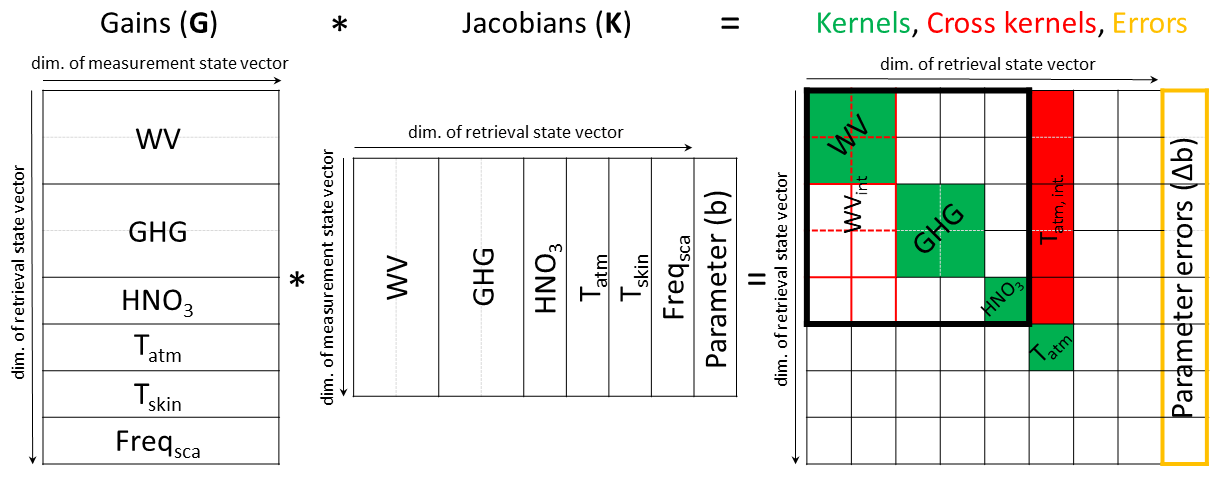
Figure 8Schematic explanation of the gain and Jacobian matrices provided in the extended netCDF output file and the kernel and cross kernel matrices (indicated as the matrix blocks filled by green and red colour, respectively) provided in all netCDF output files.
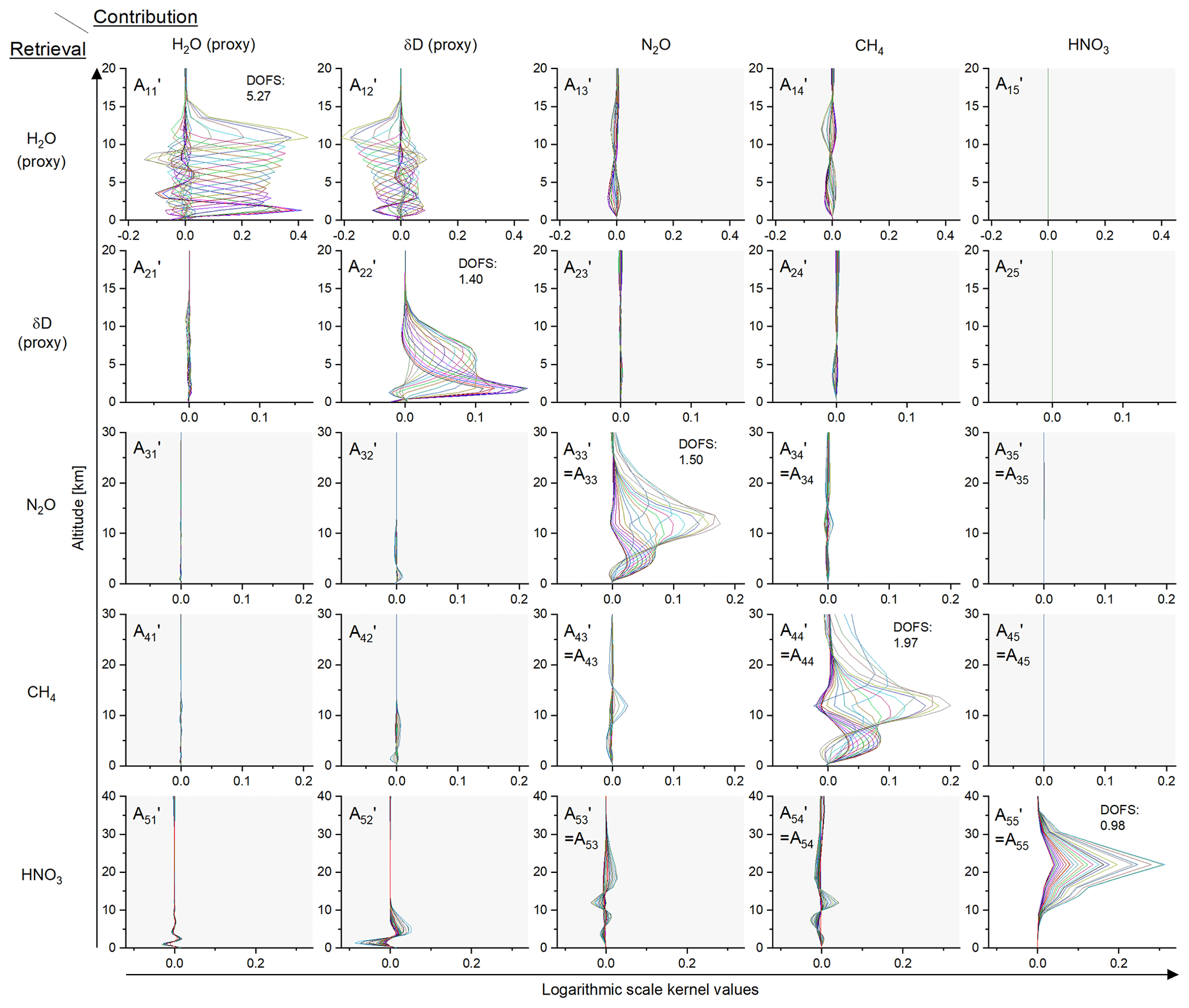
Figure 9Example of an averaging kernel for the full atmospheric composition state vector that is optimally estimated by the MUSICA IASI retrieval procedure: . The kernel is for the 30 August 2008 example observation over Lindenberg used for Fig. 4. Please note that and (ln [HDO]−ln [H2O]) are good proxies for H2O and δD, respectively.
The parts of this full matrix that are provided by the standard output files for all individual retrievals are indicated as the matrix blocks filled by green and red colour. Green represents the individual averaging kernels of the water vapour isotopologues, the greenhouse gases, HNO3, and the atmospheric temperature. Red marks the cross kernels of the trace gas products with respect to atmospheric temperature (i.e. they indicate how errors in the EUMETSAT L2 PPF atmospheric temperatures – used as MUSICA IASI a priori temperatures – affect the retrieved trace gas products). These temperature cross kernels allow the calculation of the full error covariances for the temperature uncertainty for each individual observation of the standard output file.
In addition, for all individual observations the standard output files contain square root values of the diagonal of the error covariance matrix for the most important uncertainty sources (noise and temperature uncertainty).
We always provide differential or derivatives (covariances, averaging kernels, gain matrices, and Jacobian matrices) related to the trace gas products in the logarithmic scale. Logarithmic-scale kernels are the same as the fractional kernels used in Keppens et al. (2015). Furthermore, we strongly recommend the use of the logarithmic-scale kernels for analytic calculation. Because the MUSICA IASI trace gas retrievals are made on the logarithmic scale, the assumption of a moderately non-linear case according to Rodgers (2000) can be made on the logarithmic scale (i.e. requires the use of logarithmic-scale kernels) but has limited validity on the linear scale. More details on the valid assumption of moderately non-linear problems are given in Appendix B.
5.2.1 Averaging kernels
Figure 9 depicts the averaging kernels for the full atmospheric composition state (water vapour proxy state, N2O, CH4, and HNO3) for a typical summertime observation over a mid-latitudinal land location. Shown are all the matrix blocks marked by the thick black frame in the right part of the schematic of Fig. 8. In the diagonal we see the trace gas specific kernels and in the outer diagonal blocks the cross kernels. For the H2O proxy (see Sect. 4.4.2) we achieve very high values of about 5.3 for DOFS (the degree of freedom of signal, which is calculated as the trace of the respective matrix block). Also for the δD proxy, N2O, and CH4, the DOFS values are clearly larger than 1.0, indicating the capability of the retrieval to provide some information on the trace gases' vertical distribution.
The cross kernel representing the impact of atmospheric δD on the retrieved H2O ( in Fig. 9) has the largest entries of all cross kernels; however, because variations in δD are smaller by an order of magnitude than variations in H2O, in reality this impact will be of secondary importance only. For consistency with the other data products we provide these kernels in the {ln [H2O],ln [HDO]} basis (not in the proxy basis used in Fig. 9). In the {ln [H2O],ln [HDO]} basis the cross kernels have very large and important entries, and we provide in all standard files all four blocks of the water vapour isotopologue kernels (the diagonal kernels and the cross kernels).
Similarly we also provide in all standard files all four block kernels describing the greenhouse gases (kernels A33, A34, A43, and A44 in Fig. 9). Although the respective cross kernel values are rather small, their availability supports the precise characterisation of a combined CH4–N2O product, which has a higher precision than the individual N2O and CH4 products (see discussion in García et al., 2018).
Because HNO3 has only weak spectroscopic signatures in the analysed spectral window, the respective kernel (A55 in Fig. 9) reveals a pronounced maximum, which is limited to the lower/middle stratosphere. By tuning the constraint (see discussion at the end of Sect. 4.6), we obtain DOFS values of generally close to 1.0. We also provide atmospheric temperature profile kernels (not shown in Fig. 9), for which we typically obtain a DOFS value of about 2.0.
Because we want to provide averaging kernels for each individual observation, we developed a compression procedure, which is necessary for keeping the size of the data files in an acceptable range. Section 5.2.4 describes the compression method, the format, and the variables in which the averaging kernels are provided.
5.2.2 Metrics for sensitivity and resolution
Table 2 gives an overview of metrics that can be calculated from the averaging kernel elements. In the previous section the DOFS metric has been introduced as the trace of the averaging kernel matrix. Figure 10 depicts the typical geographical distribution of the DOFS values for the different trace gas products. The largest values are generally achieved at low latitudes, except for HNO3, where we obtain the largest values at middle and high latitudes. The high values for H2O indicate that we can detect H2O profiles everywhere around the globe but in particular at low latitudes. For δD and CH4 we can also detect two independent altitude layers in the tropics and summer hemispheric subtropics. There is limited profiling capability for N2O and almost no profiling capability for HNO3. For the latter we occasionally find DOFS values of below 0.8 over the tropics, arid subtropical areas, and the central Antarctic. The DOFS values are provided in the variables with the suffix _dofs.
Table 2Metrics for sensitivity and resolution calculated from the elements of the averaging kernel matrix (Ai,j).
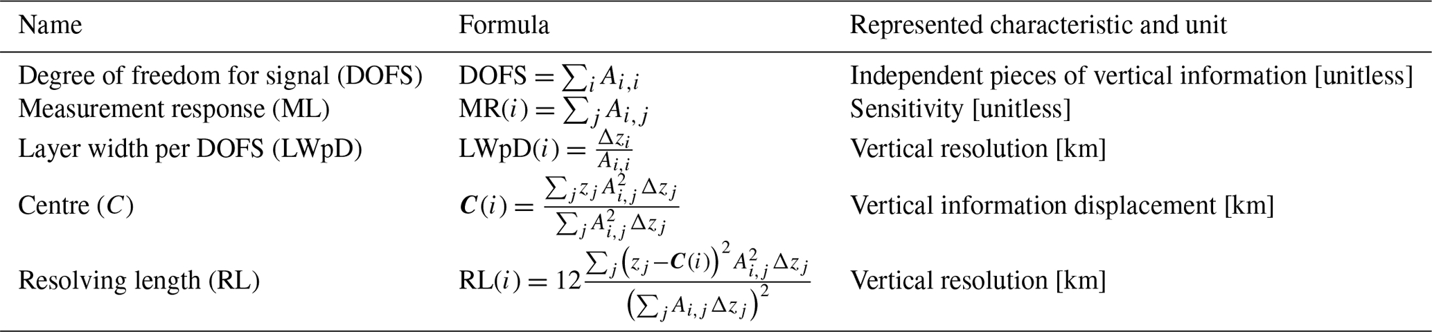
For : ; ; .
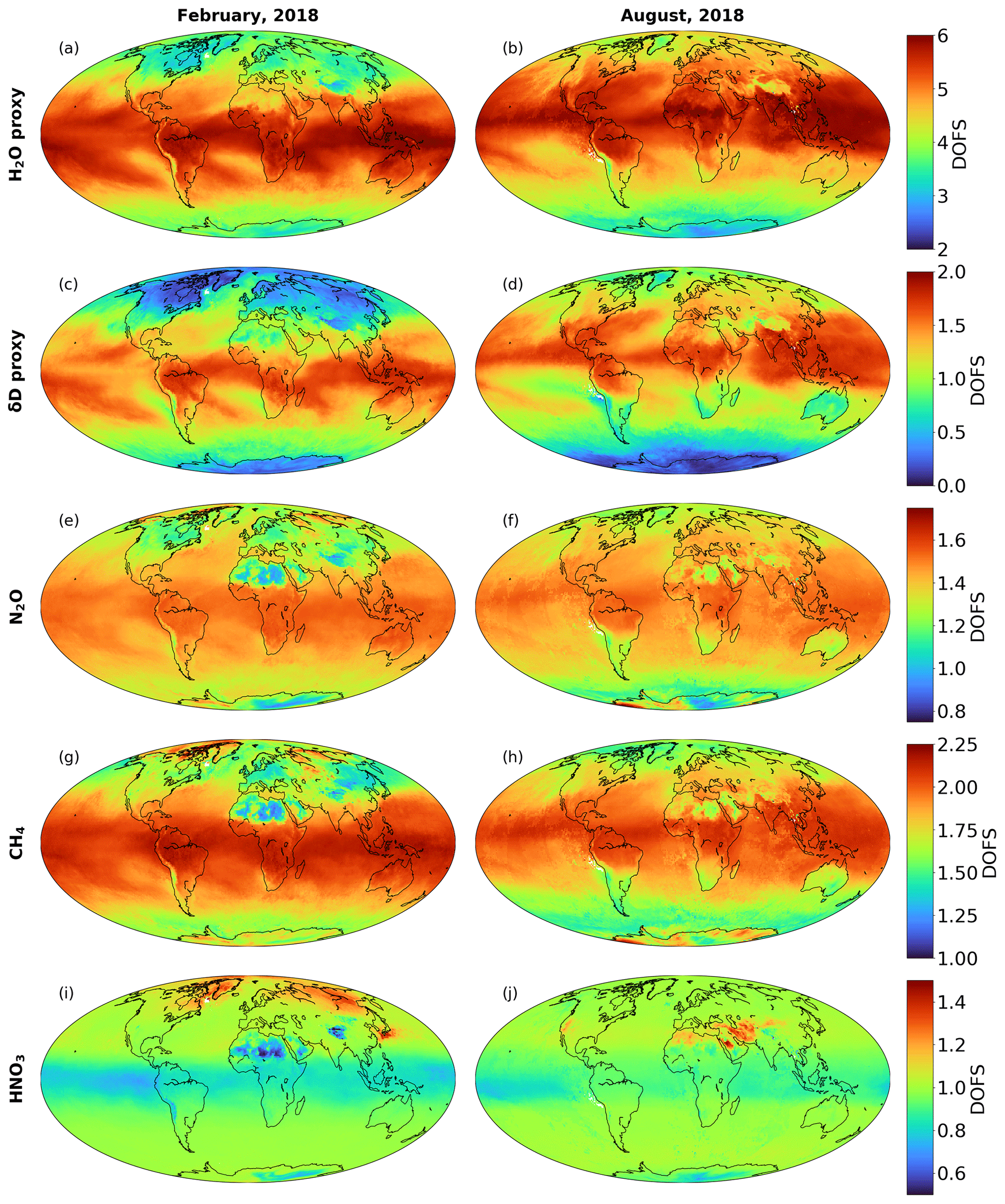
Figure 10Monthly averaged maps of degree of freedom for signal (DOFS) values for February and August 2018 for all targeted atmospheric species: H2O, δD, N2O, CH4, and HNO3.
Figure 11 shows vertical profiles of the averaging kernel metric measurement response (MR), layer width per DOFS (LWpD), information displacement (difference between the centre altitude, C, and nominal altitude, Alt), and resolving length (RL). The depicted profiles are for the averaging kernels of Fig. 9. The metrics are vectors, and each element of the vector represents a certain altitude. The equations for calculating the elements of these vectors are given in Table 2.
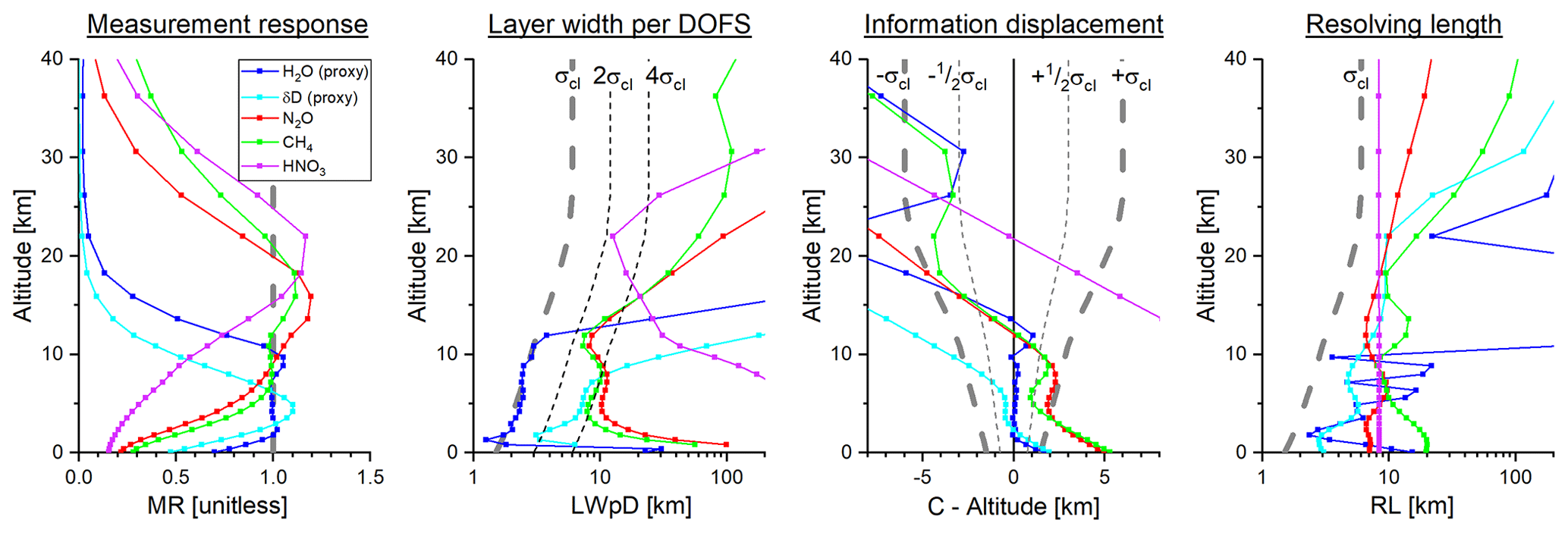
Figure 11Profiles with averaging kernel metrics for the 30 August 2008 example observation over Lindenberg used for Fig. 9. For orientation the thick dashed grey lines indicate the 100 % value (for the panel showing the measurement response) and the a priori assumed vertical correlation length (for the panels showing the layer width per DOFS, information displacement, and resolving length).
The measurement response (MR) is the sum along the row of the averaging kernel matrix (Eriksson, 2000; Baron et al., 2002). It is provided in the variables with the suffix _response. If a retrieval provides a smoothed version of the truth, without systematically pushing results towards greater or smaller values, the sum of the elements over each row of the averaging kernel should be unity. Any deviation of the row sums from unity thus hints at an influence of the constraint that is beyond pure smoothing (von Clarmann et al., 2020). Depending on the trace gas we observe different altitudes with MR values close to unity (1±0.2): tropospheric altitudes for H2O and δD, altitudes between the free troposphere and the lower stratosphere for N2O and CH4, and lower stratospheric altitudes for HNO3.
Layer width per DOFS is calculated as the local grid width divided by the respective diagonal value of the averaging kernel matrix (Purser and Huang, 1993; Keppens et al., 2015). It is a reasonable measure for vertical resolution. For our example observation we see a very good vertical resolution for H2O almost throughout the troposphere. For δD the resolution is reasonable in the lower and middle troposphere, for N2O and CH4 in the middle troposphere and upper troposphere–lower stratosphere, and for HNO3 only in a very limited altitude region in the stratosphere. Maximum values in a row of the kernel matrix away from the diagonal means that the nominal altitude and the altitude of the maximum kernel values are different. For these altitudes LWpD values strongly increase, even if the MR value is still in a reasonable range (e.g. for CH4 at about 15 km).
The centre altitude (C) indicates the atmospheric altitude region by which the retrieved values are mostly affected. In an optimal case this altitude region should correspond to the nominal altitude of the retrieval. A difference between the centre altitude and the nominal altitude (C−Alt) reveals a vertical information displacement; i.e. the signals reported by the retrieval for the nominal altitude are real atmospheric signals of a systematically different altitude. We observe very low information displacements for tropospheric H2O and middle tropospheric δD. For N2O and CH4 the values are reasonable between the middle/upper troposphere and the lowermost stratosphere. For HNO3 the centre value is almost the same for all altitudes; i.e. the signals retrieved at different altitudes reflect all the signals of the same real atmospheric altitude region.
The resolving length (RL) indicates the vertical resolution at the centre altitude, i.e. the breadth of the atmospheric altitude layer by which the retrieved value is significantly affected. As briefly discussed in Rodgers (2000) resolving length is not a satisfactory definition of resolution for slowly decaying averaging kernels or for averaging kernels that have strong side lobes, for instance the MUSICA IASI kernels for H2O (see top left panel of Fig. 9).
Resolving length and the centre altitude are calculated according to Eqs. (7) and (8) of Keppens et al. (2015). These parameters were originally introduced by Backus and Gilbert (1970) and are also discussed in chap. 3 of Rodgers (2000).
The variables with the suffix _resolution provide the vertical information displacement and resolution metrics for each individual observation. As parameters 1 and 2 these variables provide the centre altitude (C) and the resolving length (RL), respectively, and as parameter 3 the layer width per DOFS value (LWpD).
5.2.3 Errors
For the 74 observations provided in the extended output file (see Sect. 3.1) calculations of a large variety of Jacobians (and spectral responses for surface emissivity, spectroscopic parameters, and cloud coverage) and full gain matrices are available for a polar, mid-latitudinal, and tropical site (Borger et al., 2018). Figure 12 presents the errors calculated for a mid-latitudinal summer observation using the gain matrices and Jacobians (or spectral responses) according to Eqs. (A10) and (A11). The uncertainty assumption Δb and Sb used for these calculations are summarised in Table 3. The measurement noise error is calculated according to Eq. (A12) with Sy,noise being a diagonal matrix with diagonal values set to the mean-square value calculated from the spectral residuals (measured − simulated spectra).
Hess et al., 1998Hess et al., 1998Table 3List of uncertainty assumptions used for the error estimations as shown in Fig. 12.
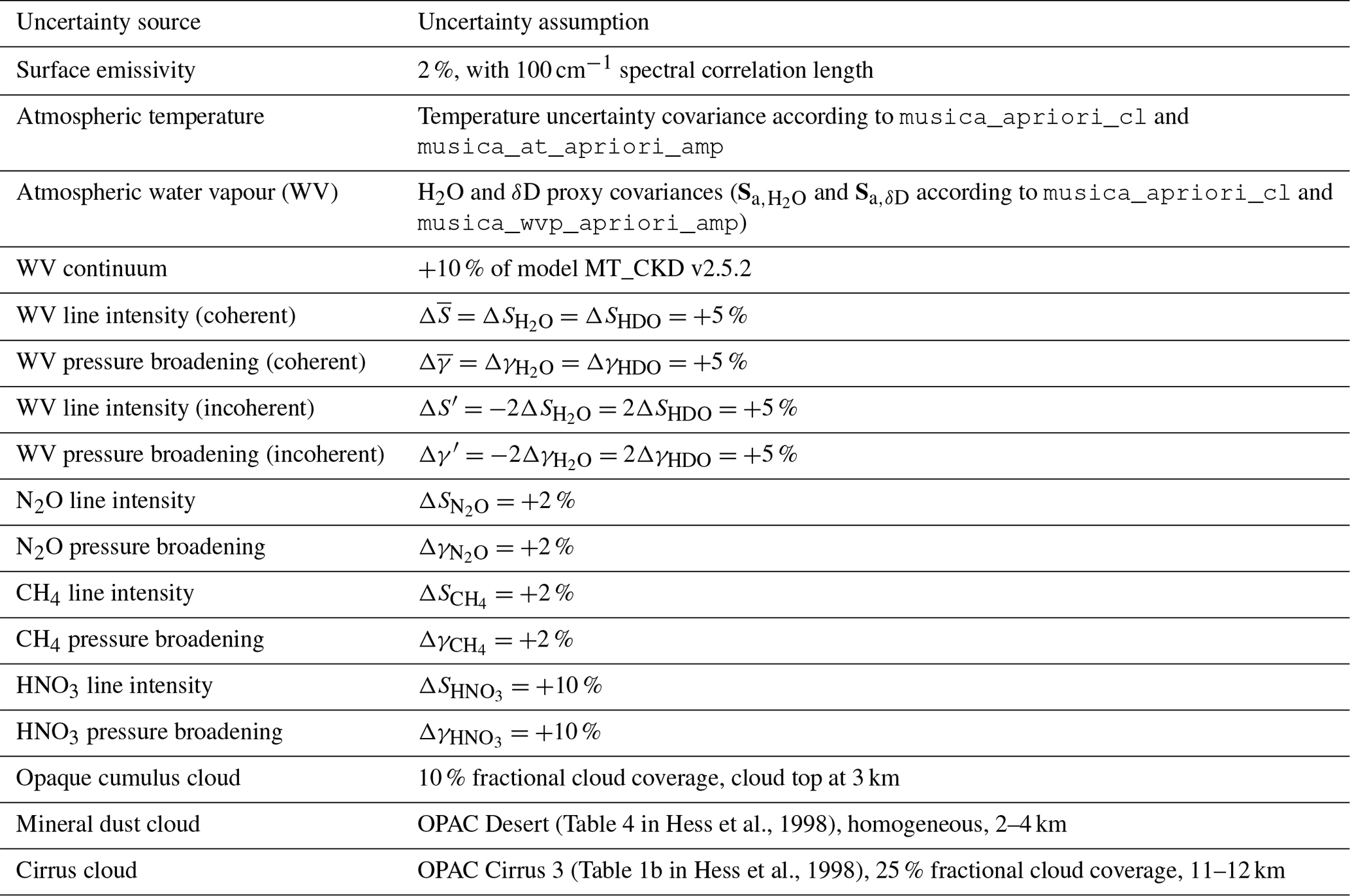
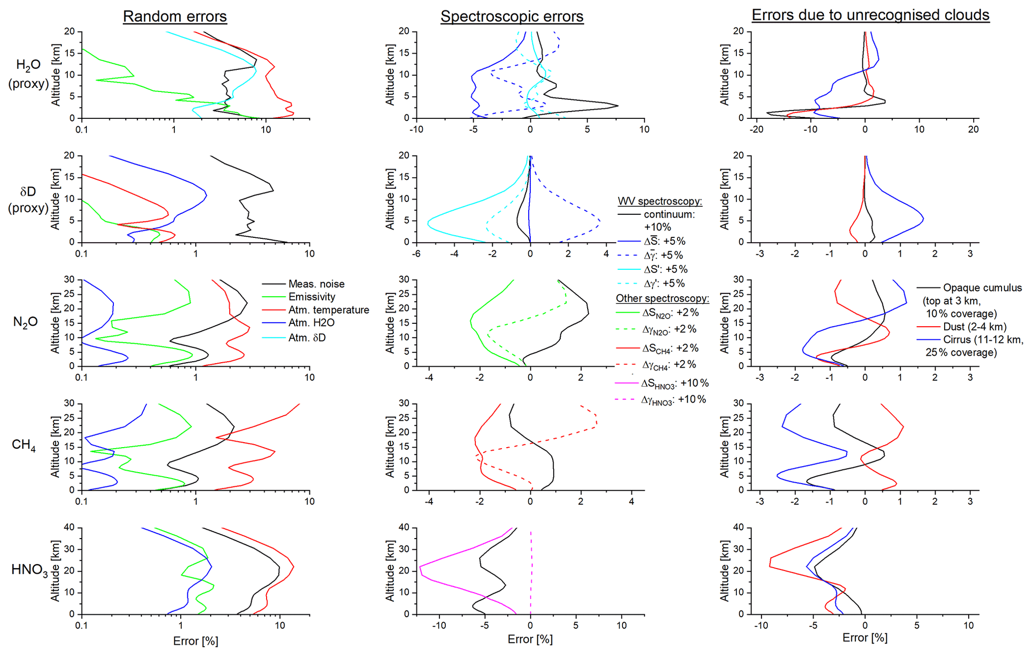
Figure 12Example of error profiles estimated for all targeted atmospheric species: H2O, δD, N2O, CH4, and HNO3. Please note that for the species H2O and δD the estimation is made for the respective proxies and (ln [HDO]−ln [H2O]). The errors are calculated according to the uncertainty assumptions of Table 3 and for the 30 August 2008 example observation over Lindenberg used for Figs. 4 and 9.
We organise the errors in three categories: random errors (measurement noise, uncertainties in emissivity and atmospheric temperature, and interferences from atmospheric humidity and δD variations), spectroscopic errors (uncertainties in the water continuum modelling and uncertainties in the intensity and pressure-broadening parameters of all target trace gases), and errors due to unrecognised clouds.
Concerning random errors, we find that atmospheric temperature uncertainties dominate the error budget for all retrieval products except for δD (because temperature uncertainties have similar impacts on H2O and HDO, they cancel out in their ratio). Measurement noise is the second most important error contributor (and the dominating error source for δD). Estimations of the dominating temperature error (assuming atmospheric temperature uncertainty covariances in line with August et al., 2012) and the measurement noise error are provided in standard files in the variables with the suffix _error, for all trace gas products (for the water vapour isotopologue in the proxy state basis) and for atmospheric temperature.
By providing the cross averaging kernels with respect to atmospheric temperature (see matrix blocks filled by red colour at the right side of the schematics of Fig. 8) we can calculate the propagation of any assumed temperature profile uncertainty ΔT individually for all observations in the standard files, according to Eq. (A10):
with KT being the Jacobians for atmospheric temperature and AT being the temperature cross kernel provided for all observations in the standard data file.
For all observations we can also reconstruct the full error covariance matrix due to the spectral noise used for constraining the solution state. For the MUSICA IASI processing we use a diagonal matrix with the mean-square values of the spectral residual (difference between the simulated and measured spectrum) as the spectral noise covariance Sy,noise. According to Eqs. (A5) to (A8) and (A12) we can write
H2O interferences from atmospheric δD and δD interferences from atmospheric H2O are also significant (blue and cyan lines in the random-error plots of Fig. 12). For this reason we provide in the standard file the four blocks of the water vapour isotopologues averaging kernels, which enables us to estimate these interferences for each individual observation. The error covariance due to interference of δD on H2O can be calculated by
and the error due to interference of H2O on δD by
Here Sa,δD and are covariances of the δD and H2O proxy states, respectively, and and are the cross kernels of the proxy states. Please note that the water vapour isotopologue kernels provided in the standard files are for the {ln [H2O],ln [HDO])} basis and not for the {,(ln [HDO]−ln [H2O])} proxy state basis; i.e. to be used according to Eqs. (17) and (18) the provided kernels have to be transformed according to Eq. (4).
Spectroscopic uncertainties cause mainly systematic errors. The assumed uncertainties in line intensity ΔS and pressure-broadening Δγ (see Table 3) are in reasonable agreement with the values reported in Gordon et al. (2017). Respective error estimations can be performed for the 74 exemplary observations provided in the extended data file over a polar, mid-latitudinal, and tropical site. As shown in Fig. 12 they are typically within 5 %, except for HNO3, where we estimate errors in the lower stratosphere due to spectroscopic uncertainties of up to 12 % (mainly reflecting the larger uncertainty budget allowed for the band intensity). The uncertainties in the spectroscopic parameters of line intensity and pressure broadening mainly affect the retrieval of the trace gas, for which the parameters are assumed to be uncertain. Cross impacts are largest for uncertainties in water vapour parameters and there mostly for the water continuum (to a lesser extent for line intensity and pressure broadening). For this reason we plot the effect of the water continuum uncertainty for all trace gases, whereas we only show the effects of the line intensity and pressure-broadening parameters of the trace gas that is examined.
MUSICA IASI retrievals are only executed when the EUMETSAT L2 PPF flag flag_cldnes is set to 1 (the IASI instrumental field of view, IFOV, is clear) or 2 (the IASI IFOV is processed as cloud-free, but small cloud contamination is possible). This means that in particular for MUSICA IASI retrievals made with a cloud flag value of 2, clouds can have an impact, which should be examined. For this reason we calculated a variety of different cloud spectral responses for our 74 exemplary observations over polar, mid-latitudinal, and tropical sites and provide them in the extended data files. Examples of the obtained errors are depicted on the right of Fig. 12. We find that clouds with the properties as described in Table 3 have a significant effect on the retrievals. The impact of a cirrus cloud is particularly strong, and the H2O and HNO3 data products seem to be the most affected. However, in this context we also have to consider the natural variability in the different trace gas products. Because the natural variability in δD, N2O, and CH4 is very small, uncertainties due to clouds of 1 % can already be a large problem. In summary this estimation of errors due to unrecognised clouds indicates that we should be careful when using MUSICA IASI data products corresponding to an EUMETSAT L2 PPF cloud flag value of 2 (see also discussion in Sects. 6 and 7).
5.2.4 Matrix compression
In order to reduce the storage needs of the output files, we compress the averaging kernel matrices. For this compression we perform a singular value decomposition of the original averaging kernel
and a subsequent filtering for the leading eigenvalues. We only keep the most important eigenvalues and eigenvectors; i.e. we only keep a small part of the matrices U, D, and V. The variables that store this leading information on the averaging kernels have specific suffixes in their names. The variable with suffix _avk_rank stores the number (r) of the leading eigenvalues and eigenvectors that are kept. Suffix _avk_val identifies the variable containing the eigenvalues. The variables with suffixes _avk_lvec and _avk_rvec store the leading left and right eigenvectors. The reconstruction of the averaging kernel is made according to Eq. (19), whereby we setup the r×r diagonal matrix D consisting of the leading eigenvalues and the n×r matrices U and V consisting of the leading left and right eigenvectors. Here n is the numbers of elements in the considered state vector. When reconstructing all four blocks of the water vapour or greenhouse gas averaging kernels, . For the reconstruction of the HNO3 or atmospheric temperature averaging kernels n=nal. For more details on the effectiveness of this compression method please refer to Weber (2019).
The suffixes _xavkat_rank, _xavkat_val, _xavkat_lvec, and _xavkat_rvec identify the respective variables needed for the reconstruction of the temperature cross averaging kernels. In this case the right eigenvectors have the length of the atmospheric temperature state vector, which is different from the length of the atmospheric state vector in the case of the water vapour isotopologue and the greenhouse gas product (i.e. for the water vapour isotopologue and the greenhouse gas temperature cross averaging kernels, the left and right eigenvectors have different sizes).
The MUSICA IASI retrieval data are provided with detailed information on the retrieval quality, the retrieval products' characteristics, and errors, as well as variables summarising cloud conditions and the main aspects of sensitivity, vertical resolution, and errors. In this section we discuss the variables providing this information and recommend possibilities for data filtering.
6.1 Clouds
The EUMETSAT L2 PPF flag flag_cldnes is written in the MUSICA IASI variable eumetsat_cloud_summary_flag. As discussed in Sect. 5.2.3 there is some risk that the MUSICA IASI product retrieved for eumetsat_cloud_summary_flag set to 2 has significant errors due to clouds. In order to exclude this risk we can filter out these data; i.e. we can use a very stringent cloud filtering criterion by using only observations where the variable eumetsat_cloud_summary_flag is set to 1.
Another and less stringent option is to use in addition the EUMETSAT L2 fractional cloud cover, which is written in the MUSICA IASI variable eumetsat_cloud_area_fraction. If eumetsat_cloud_summary_flag is set to 2 we require in addition that the determination of a cloud area fraction has not been successful; i.e. we require that eumetsat_cloud_area_fraction is set to NaN. No clear determination of a value for fractional cloud cover means that the cloud signals are rather weak (the contrast between cloud and surface signals is smaller than the instrument noise).
6.2 Quality of the spectral fit
The spectral noise level considered in the cost function Eq. (A2) during the MUSICA IASI processing is the root-mean square (rms) of the spectral fit residual (difference between the simulated and measured spectrum). By this retrieval setting we use the degree to which the spectra can be understood by the forward model as the spectral noise level. The so-defined spectral noise level is generally larger than the pure instrumental noise level because it is a sum of the instrumental noise and the signatures that are not understood by the forward model. In the MUSICA IASI retrieval this rms value is treated as white noise; i.e. for Sy,noise of the cost function Eq. (A2) we use a diagonal matrix filled by the mean-square values according to the spectral residuals.
As long as the residual is close to white noise, this kind of processing ensures a correct weighting of the measured spectra, on the one hand, and the a priori information, on the other hand. However, occasionally the measured spectra are very poorly simulated by the forward model and the residuals cannot be described as white noise; instead the residuals show systematic signatures. This happens, for instance, if incorrect surface emissivities are used or if the retrieval is made for an observation that is affected by a cloud. In order to identify the systematic part of the residuals we smooth the residuals using a ±2 cm−1 running mean. The smoothed residuals are the systematic residuals, and the difference between the original residuals and the smoothed residuals can then be interpreted as the random (or white noise) residuals. Residuals, systematic residuals, and random residuals are provided in the standard files for each observation in the variable
musica_fit_quality.
In order to facilitate the filtering of data corresponding to a poor spectral fit quality, we set up a flag (provided as variable musica_fit_quality_flag) that works with the rms values of the systematic residuals and the random residuals. The flag is set to 0 (poor quality) if the systematic residuals have an rms value of larger than 40 nW/(cm2 sr cm−1). For all other observations we analyse the ratio between the rms of the systematic residuals and the rms of the random residuals. If this ratio is larger than 1.0, the flag is set to 1 (restricted quality); if it is between 0.5 and 1.0, the flag is set to 2 (fair quality); and if it is smaller than or equal to 0.5, the flag is set to 3 (good quality). Figure 13 depicts residuals corresponding to different values of this fit quality flag. All observations are made during the same orbit, at close-by locations (northern Africa), and for very similar surface temperatures. It is very likely that the poor spectral fit quality is due to incorrect surface emissivity values used for the respective retrievals (over arid areas like northern Africa, surface emissivity data have an increased uncertainty; Seemann et al., 2008). Our recommendation is to use data that belong to the quality groups fair and good.
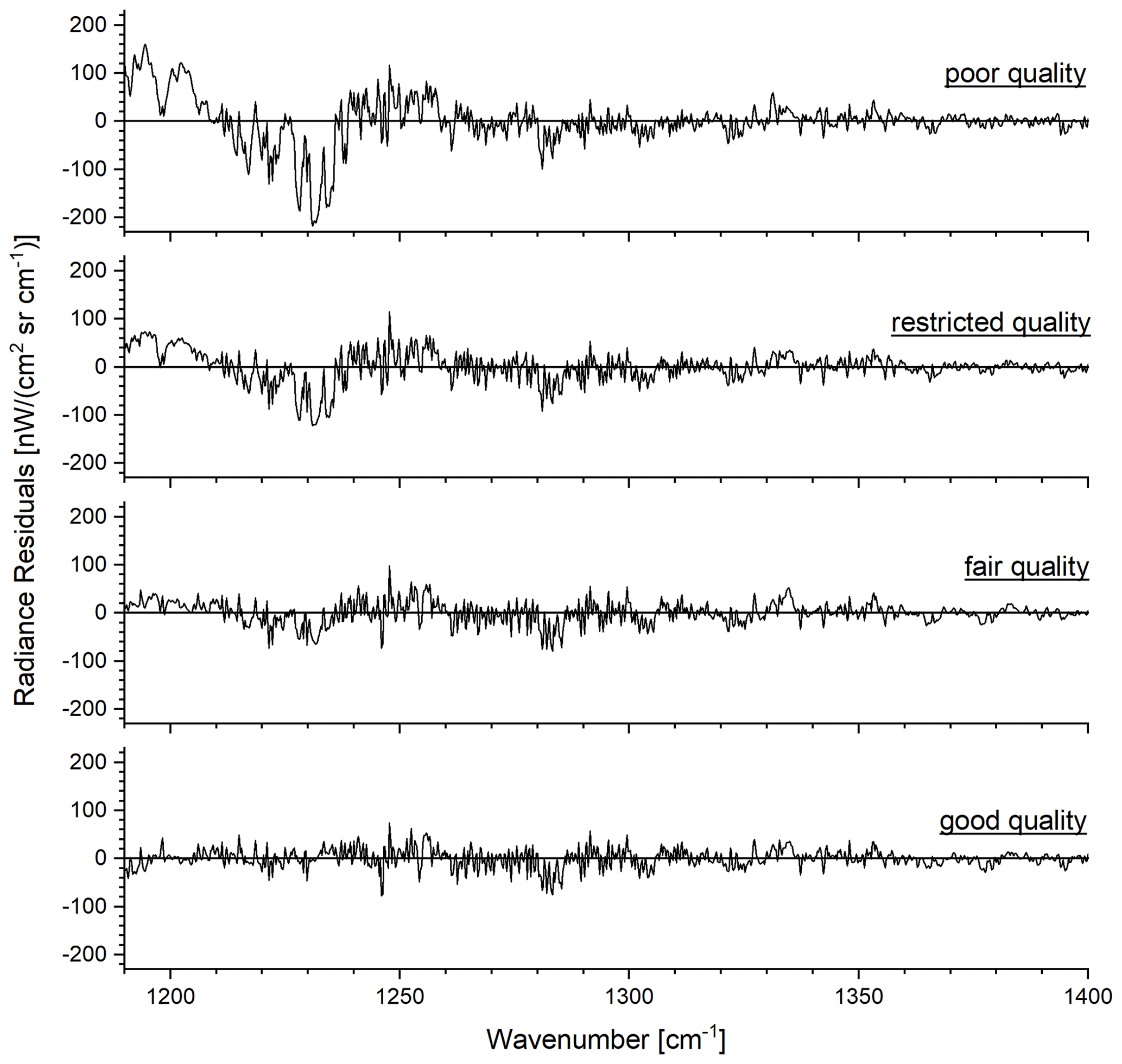
Figure 13Example of residuals (simulated − measured spectra) belonging to the different quality groups as documented by the variable musica_fit_quality_flag: poor, restricted, fair, and good. The retrievals correspond to observations over northern Africa with relatively high but very similar surface skin temperature (319.1–319.3 K) made during the Metop-A orbit no. 51267 as shown on the left of Fig. B1.
6.3 Errors
For all observations and all trace gas products, the standard files provide estimations of the errors dominating the random-error budget: errors due to noise in the spectra and errors due to uncertainties in the atmospheric temperature a priori data (the EUMETSAT L2 PPF temperatures). The noise error and estimations of atmospheric temperature error are given in the error variable (variable with suffix _error; see Sect. 5.2.3) for all trace gas products and can be used for filtering out data with anomalously high errors.
Incorrect spectroscopic parameters (line intensity, pressure-broadening coefficients, or water continuum modelling) can be responsible for large errors. Although these uncertainty sources are systematic, the errors they cause depend on the sensitivity of the remote sensing system, which in turn is affected by the geometry of the observation. In the first order the optical path of the measured radiances depends on the platform zenith angle (PZA, provided as the variable platform_zenith_angle). In order to avoid that systematic uncertainties in the spectroscopic parameters cause artificial signals, we can set threshold values for the PZA and limit the PZA to angles close to nadir (e.g. by requiring ).
6.4 Sensitivity and resolution
The standard files provide the averaging kernels in a compressed format for all observations (see Sect. 5.2.4) as well as metrics that capture the most important aspects of the sensitivity and vertical resolution (see Sect. 5.2.2). These metrics are provided in the variables with the suffixes _response and _resolution and allow analyses of the sensitivity and vertical resolution for each individual observation without the need for reconstructing the averaging kernels. We can use the metrics for filtering out data where the response to the real atmospheric variability is low or where the vertical representativeness is irregular.
In order to ensure a good sensitivity (retrieval product being mainly affected by the real atmosphere and not by the a priori assumption), the measurement response (MR) should be close to unity. Layer width per DOFS (LWpD), centre altitude displacement (C−Alt), and resolving length (RL) can be used to filter out data that do not fulfil the requirements in terms of the vertical representativeness needed for a dedicated study. Respective filter threshold values depend on the objective of the scientific study. If processes within vertically well confined layers shall be examined, rather small vertical displacement and very good vertical resolution are required, and thus very stringent thresholds should be set.
In addition to filtering according to absolute values of LWpD, C−Alt, or RL, the respective metrics can also be used for the identification of groups of data that have a similar vertical representativeness. For instance, we can robustly analyse time series of data that have a stable vertical information displacement and a stable vertical resolution. For data where these conditions are not fulfilled, time series signals might be significantly affected by the time-variant data characteristics. The same is true when analysing horizontal patterns, which might partly be due to the pattern in the data characteristics and not a real atmospheric pattern.
Each Metop satellite accomplishes about 14 orbits per day, which makes about 5100 orbits per year. For our MUSICA IASI retrieval period there are two or even three orbiting IASI instruments making operational measurements. Until the end of October 2019 there were IASI-A and IASI-B, and since November 2019 there has been in addition IASI-C. So we have more than 10 000 Metop–IASI orbits and in consequence MUSICA IASI netCDF output files per year with useful measurements (see Sect. 3.1 for information on output data file nomenclature and format).
As an average about 30 % of all measurements are made for cloud-free conditions (EUMETSAT L2 PPF cloudiness assessment summary flag set to 1 or 2; see also Sect. 4.1). This makes about 25 000 individual retrievals per orbit/output file. In the following we present examples of this large number of data. We select example altitudes where the respective products have generally a good sensitivity and reasonable vertical representativeness. According to Figs. 9 and 11 a good altitude choice is 4.2 km for H2O and δD and 10.9 km for N2O and CH4. For HNO3 the MUSICA IASI processor does not provide profile information; instead the kernels for all altitudes show a similar vertical dependence and reveal retrieval sensitivity for a broad lower stratospheric layer. For this reason we aggregate the HNO3 data in the form of partial column-averaged mixing ratios for the layer between 10 and 35 km. Details on this resampling are given in Appendix C.
7.1 Filtering
We filter the data according to the settings and threshold values of Table 4. For all data we require “fair” and “good” for the MUSICA IASI spectral fit quality (flag variable musica_fit_quality_flag is required to be set to 2 or 3), and we filter the data using the EUMETSAT L2 PPF cloudiness assessment flag (provided as the variable eumetsat_cloud_summary_flag).
For the N2O and CH4 data we apply a more stringent cloud filter and further inspect data where the EUMETSAT L2 PPF cloudiness assessment summary flag indicates a possibility of small cloud contamination. For respective data we require that the EUMETSAT L2 processing cannot clearly attribute a value for fractional cloud cover, which means that the cloud signals are rather weak (see Sect. 6.1). We use this more stringent cloud filtering for N2O and CH4 because both species have relatively weak atmospheric variabilities that are very similar to the errors estimated for a small cloud coverage (10 % coverage with opaque cumulus clouds or 25 % coverage with cirrus clouds).
Table 4Filters applied for the time series and global daily maps of different species and for different altitudes (Alt) as shown in Figs. 14 and 15: EUMETSAT L2 PPF cloudiness assessment summary flag, MUSICA spectral fit quality flag, platform, zenith angle, MUSICA noise and temperature error, and MUSICA averaging kernel metrics (measurement response: MR; diagonal value of the partial column averaging kernel: ; altitude layer width per DOFS: LWpD; vertical information displacement: C−Alt).
a Only if variable eumetsat_cloud_area_fraction is set to NaN. b For dry-air mixing ratios averaged for partial column 10–35 km a.s.l. c Here the bottom thresholds are set to be below the lowest actually occurring positive value.
Furthermore, we filter according to the retrieval fit noise and estimated atmospheric temperature errors. The respective errors are provided for each observation in the MUSICA IASI standard file output variables with the suffix _error. For HNO3 we calculate the retrieval fit noise and the estimated temperature errors for the 10–35 km partial column-averaged mixing ratios according to Eq. (C7), whereby we reconstruct the noise covariance matrix for HNO3 according to Eq. (16) and generate the atmospheric temperature covariance according to Eq. (7) using the MUSICA IASI standard file output variables musica_at_apriori_amp and musica_apriori_cl for setting up the values of
vamp,i and σcl,i, respectively.
In order to ensure that the time series signals or horizontal patterns are not significantly affected by varying sensitivity and vertical resolution, we filter H2O, δD, N2O, and CH4 data according to the averaging kernel metrics MR, LWpD, and C−Alt. This filters out data with anomalous vertical sensitivities. For HNO3 we calculate the 10–35 km partial column-averaged mixing ratio averaging kernels according to Eq. (C6) and filter for good sensitivity by requiring a diagonal entry close to unity.
The filter threshold values of LWpD and C−Alt are defined relative to the a priori assumed vertical correlation length (provided in the variable musica_apriori_cl). We use threshold values for these ratios that are constant for all altitudes, which allows for increased LWpD and C−Alt values in the case of an increased vertical correlation length (for altitudes with a larger correlation length, higher values of LWpD andC−Alt can be accepted).
7.2 Continuous time series
In this section we give an example of the temporal continuity of the data. Figure 14 depicts a time series at the mid-latitudinal site of Karlsruhe, Germany, between October 2014 and June 2021 of MUSICA IASI trace gas retrieval products. For all trace gases, except for δD, we have good temporal coverage with no significant data gaps caused by the comprehensive data filtering. Concerning δD, there is a reduced data volume in winter mainly due to filtering out data with reduced sensitivity (measurement response below 0.8). It is worth noting that for the {H2O, δD} pair optimal estimation product – generated a posteriori according to Diekmann et al. (2021) – we achieve a significantly better measurement response.
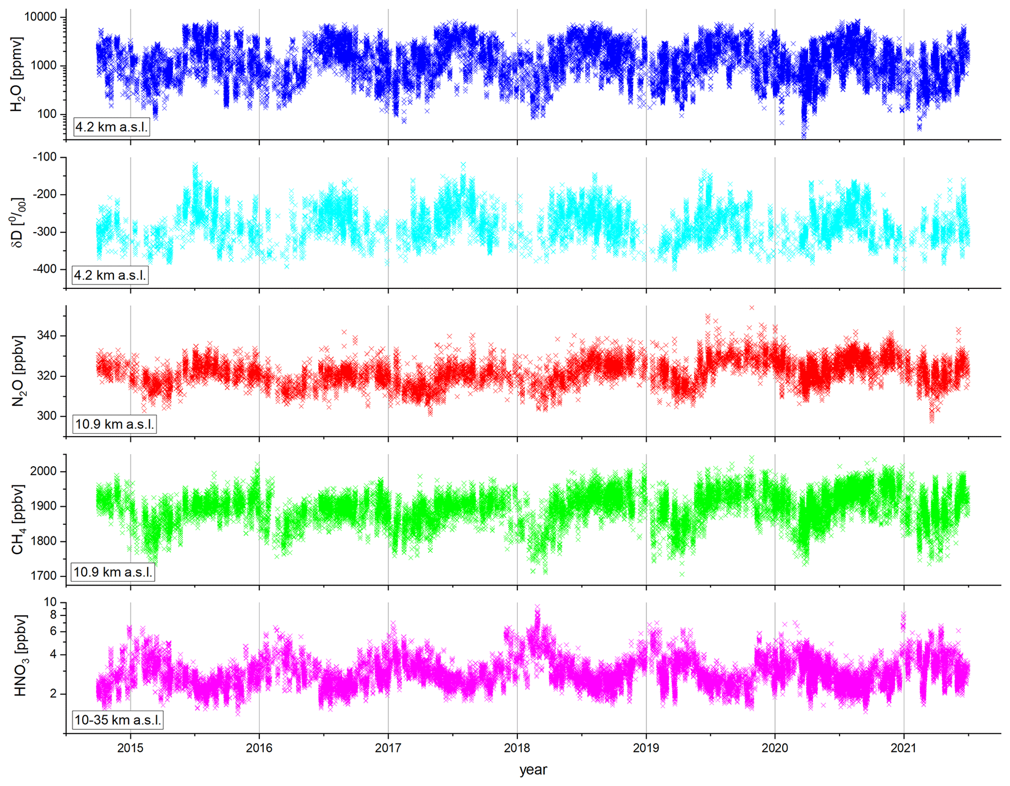
Figure 14Time series of MUSICA IASI trace gas products at selected altitudes above Karlsruhe (48–49∘ N, 8–9∘ E): 4.2 km a.s.l. for H2O and δD, 10.9 km a.s.l. for N2O and CH4, and 10–35 km a.s.l. for HNO3. Data have been filtered according to the settings given in Table 4.
We observe typical seasonal cycles for all species. The seasonal cycles of H2O and δD follow the seasonal cycle of temperature. In winter H2O concentrations can be as low as 100 ppm and δD values can be below −350 ‰. In summer the maximum values are about 8000 ppm and −150 ‰. The concentrations of N2O and CH4 at 10.9 km a.s.l. are lowest in winter–spring and highest in summer–autumn. This cycle is linked to the vertical shift of the tropopause altitude: in winter–spring the 10.9 km altitude is much more strongly affected by the stratosphere (where N2O and CH4 are decreasing with height) than in summer–autumn. Concerning HNO3 we observe the highest values in winter–spring, which might indicate the detection of air masses with an Arctic stratospheric history (Arctic winter stratospheric HNO3 mixing ratios are particularly large).
7.3 Daily global maps
In this section we give an example of the good daily global coverage achieved by high-quality MUSICA IASI products. Figure 15 depicts the data retained during 24 h when using the filter setting listed in Table 4. For our example we choose 1 February and 1 August 2018 and plot the data for the same altitudes as in Fig. 14. For all data products, except for δD, we have very dense global coverage. Areas with missing data are mostly linked to the cloud filtering. The reduced data coverage for δD in the middle and high latitudinal winter hemispheres is due to δD measurement response values lying below 0.8 (we achieve a significantly better measurement response and thus horizontal coverage for the optimal estimation {H2O,δD} pair product generated according to Diekmann et al., 2021).
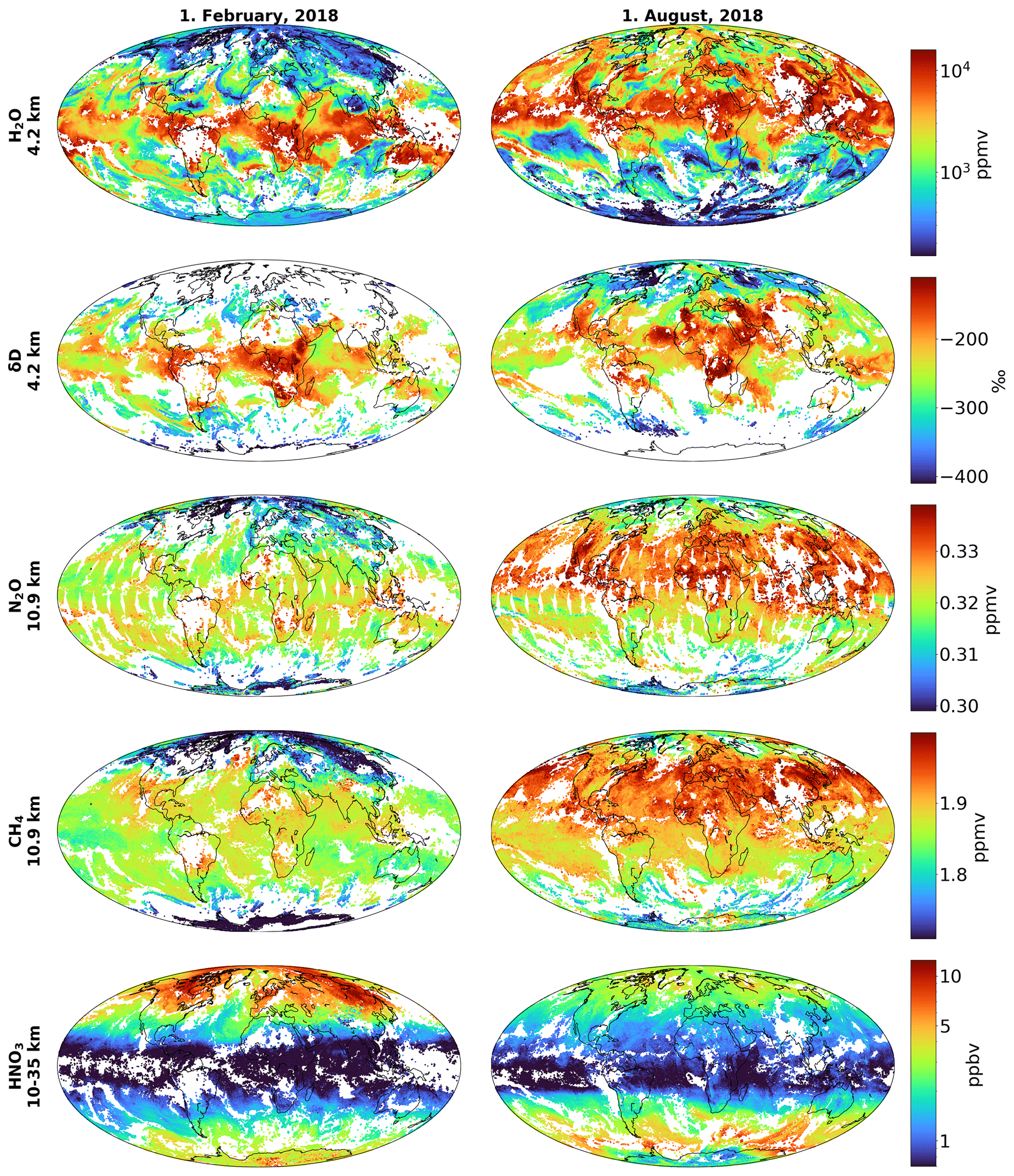
Figure 15Daily maps for 1 February and 1 August 2018 of the trace gas products for the same altitudes as in Fig. 14. Altitude 4.2 km a.s.l. for H2O and δD, 10.9 km a.s.l. for N2O and CH4, and 10–35 km a.s.l. for HNO3. Data have been filtered according to the filter settings given in Table 4 (same as for Fig. 14).
The highest H2O concentrations at 4.2 km are observed at low latitudes where temperatures are generally highest. However, there are also low latitudinal areas with rather low H2O concentrations, for instance in the eastern Pacific on 1 August 2018, which indicates a region where large-scale subsidence is prevailing. The δD values at 4.2 km are also highest at low latitudes but with a stronger zonal variability. For high tropical H2O concentrations, δD values can be relatively high (for instance on 1 February 2018 in the tropical Atlantic) or relatively low (for instance on 1 February 2018 in the tropical Indian Ocean). This indicates that δD data contain information that is complementary to the H2O data.
For N2O and CH4 at 10.9 km we observe maximum concentrations at low latitudes and rather low values in the polar regions. The reason for this is that at high latitudes the 10.9 km altitude is strongly influenced by low stratospheric concentrations, whereas in the tropics the 10.9 km altitude is representative of the upper troposphere, where concentrations are higher. This means that the concentrations observed at 10.9 km reflect to a large extent the altitude of the tropopause. On 1 August 2018 we observe for both trace gases a clear gradient between the Northern Hemisphere and Southern Hemisphere, whereas there is no significant gradient on 1 February 2018. This is caused by higher tropospheric concentrations of both trace gases in the Northern Hemisphere. On 1 August 2018 the stratosphere affects the 10.9 km altitude more strongly in the Southern Hemisphere than in the Northern Hemisphere and we observe particularly strong gradients. On 1 February 2018 it is the other way round and the tropospheric concentration gradients are counterbalanced by the tropopause altitude effect.
The global maps of the HNO3 10–35 km partial column-averaged mixing ratios show very low values in the tropics and the highest values in polar regions. However, in the Antarctic low values are also found in winter because at very low temperatures (<195 K) polar stratospheric clouds (PSCs) are formed on which HNO3 condensates. In the Arctic winter temperatures are generally not that low and PSCs and consequently low HNO3 values are mainly restricted to areas with a local mountain lee wave occurrence.
For each individual observation, the MUSICA IASI full retrieval product provides detailed information on retrieval settings (a priori and constraints) and retrieval characteristics (error covariances and averaging kernels). This comprehensive set of information ensures ultimate interoperability and offers the possibility of a variety of data reuse applications, in particular, because the MUSICA IASI inversion problem is a moderately non-linear problem (see Appendix B). In the following we briefly list some data reusage possibilities.
For interoperability (the common use of different data sets or their inter-comparison) the impact of different a priori data should be assessed or eliminated. Assuming that the MUSICA IASI data (generated using a priori state xa) should be commonly used with (or inter-compared to) another remote sensing data set whose retrieval processor used the a priori state xa,m, then we can calculate the MUSICA IASI retrieval state that would result from an xa,m a priori usage according to Eq. (B1). For these calculations we need, from the MUSICA IASI data, the originally retrieved state, the a priori state, and the averaging kernels, which are all provided by the MUSICA IASI full retrieval product.
For comparisons to atmospheric model simulation or for data assimilation applications, a remote sensing product has to be made available together with full information about its error covariances and measurement operator. This is the case for the MUSICA IASI full retrieval product data set. For each individual observation the averaging kernels are made available and the full a posteriori covariances and the error covariances due to the fit residuals can be reconstructed from the provided constraint and the averaging kernel matrices according to Eqs. (A7) and (16), respectively.
As shown in Sect. 7 and Appendix C the MUSICA IASI trace gas profiles can be easily resampled according to user-specific needs in the form of partial column-averaged mixing ratios with corresponding averaging kernels and error covariances. This is possible because the data set provides full information on pressure profiles, constraints (for reconstructing the error covariances due to the corresponding fit residuals, see Eq. 16), temperature cross kernels AT (in order to calculate the error covariances due to atmospheric temperature uncertainties, see Eq. 15), and averaging kernels.
Worden et al. (2012) and García et al. (2018) discussed the advantages of a ratio product. García et al. (2018) showed that this ratio product has a theoretically higher precision than the individual N2O and CH4 products. Because N2O is chemically more stable than CH4 in the troposphere, it is also more homogeneously distributed than CH4. García et al. (2018) argued that by combining ratio observations with a model of the N2O climatology, it should be possible to determine tropospheric CH4 concentration with relatively high precision. The MUSICA IASI full retrieval product provides information on constraints and the averaging kernels (including the cross averaging kernels between N2O and CH4); thus it offers all that is needed for calculating the ratio product as well as the corresponding averaging kernels and error covariances.
Another interesting data reuse possibility is that the retrievals' a priori data or the retrievals' constraints can be modified a posteriori in accordance to particular user requirements. According to Eq. (18) of Rodgers and Connor (2003), we can calculate the retrieval result () for a modified constraint (Rm) by
Here xa, A, , and are the a priori state, the averaging kernel, the error covariance due to retrieval fit noise, and the originally retrieved state, respectively. All this information is made available in (or can be reconstructed from the information provided by) the MUSICA IASI full retrieval product. Diekmann et al. (2021) present an optimal estimation {H2O,δD} pair product, which among others makes use of such a posteriori constraint modification.
Schneider et al. (2021c) present another possibility for MUSICA IASI data reuse. They apply the extensive information provided in the MUSICA IASI full retrieval product for optimally combining MUSICA IASI CH4 data with the total column XCH4 retrieval products of the sensor TROPOMI (TROPOspheric Monitoring Instrument) aboard the satellite Sentinel-5P (Lorente et al., 2021) without the need for running new retrievals. This a posteriori product combination can be achieved by Kalman filter calculations (Kalman, 1960; Rodgers, 2000), which have large similarities to Eq. (20). The method optimally combines the MUSICA IASI retrieval state (vector ) with the information provided by the TROPOMI XCH4 product (the scalar ; we use index n for new observation):
Here the vector is the optimally combined state, the row vector is the column averaging kernel of the TROPOMI XCH4 observation, the scalar xa is the a priori XCH4 data, and the vector xa is the a priori CH4 profile. is the a posteriori covariance of the MUSICA IASI data, which can be reconstructed with averaging kernel and constraint matrices being available according to Eq. (A7). The scalar is the measurement noise error variance of the TROPOMI XCH4 product. Optimal means here that the uncertainties and sensitivities of the MUSICA IASI CH4 product and the TROPOMI XCH4 product are correctly taken into account.
The MUSICA IASI data can be freely downloaded at http://www.imk-asf.kit.edu/english/musica-data.php (last access: 25 January 2022). We offer two data packages with DOIs. The first data package has a data volume of about 17.5 GB and is linked to via https://doi.org/10.35097/408 (Schneider et al., 2021b). It contains example standard output data files for all MUSICA IASI retrievals made for a single day (more than 0.6 million) and a description of how to access the total data set (2014–2019, data volume 25 TB) or parts of it. This data package is for users interested in the typical global daily data coverage and in information about how to download the large data volumes of global daily data for longer periods. The second data package contains the extended output data file, is only about 73 MB, and is linked to via https://doi.org/10.35097/412 (Schneider et al., 2021a). It contains retrieval products for only 74 observations made at a polar, mid-latitudinal, and tropical location. It provides the same variables as the standard output files and in addition the variables with the prefixes musica_jac_ and musica_gain_, which are Jacobians (or spectral responses) for many different uncertainty sources and gain matrices (due to these additional variables it is called the extended output file). Because this data package is rather small, it is recommended to potential reviewers and to users for having a quick look at the data.
MUSICA IASI data processing is ongoing. For IASI observations after June 2019 the MUSICA IASI processing versions 3.3.0 and 3.3.1 instead of 3.2.1 are used (the differences between the versions 3.2.1 and 3.3.x are of a technical nature and not noticeable by the data user). Data representing observations after 2019 will soon be made available to the public in the same format as the data presented here (such data are already depicted in Fig. 14).
Measurements of the IASI instruments on the three satellites Metop-A, Metop-B, and Metop-C have been processed by the MUSICA IASI processor. The processing has been made globally for all measurements that are declared as likely cloud-free by the EUMETSAT L2 PPF cloud detection procedure. Here we report on the full retrieval product of the MUSICA IASI processing version 3.2.1 used for the observation time period between October 2014 and June 2019. This report is equally valid for version 3.3.x data (in use for observations after June 2019.)
The full retrieval product is the comprehensive output of the main MUSICA IASI processing chain. It contains the simulated and the residual radiances (the difference between measured and simulated radiances), some flags and retrieval outputs provided by the EUMETSAT L2 PPF processing, full information on the MUSICA IASI retrieval settings, and the full MUSICA IASI retrieval output. For each observation we provide information on the MUSICA IASI a priori settings and constraints so that the data are very easily reproducible. The retrieval outputs are the trace gas profiles of H2O, HDO, N2O, CH4, and HNO3 as well as the atmospheric temperature profiles. Concerning H2O and HDO the retrieval is optimised for H2O and the ratio of . All products are provided with a very extensive characterisation. For each individual retrieval the leading errors are made available together with the averaging kernels. In order to reduce the data volume, the kernels are provided in a compressed data format and can be reconstructed by simple matrix calculations. In addition we provide variables with averaging kernels metrics that capture the most important characteristics of the vertical representativeness (sensitivity and vertical resolution). These variables can be used for identifying data with an acceptable vertical representativeness without the need for reconstructing the averaging kernels. We give some suggestions on how to use different flags, error information, and averaging kernel metrics for data filtering recommendable for the study of global distribution maps or time series.
The output of a priori states and averaging kernels for each individual observation guarantees ultimate interoperability (the common use of different data sets or their inter-comparison). Furthermore, the additional supply of constraint matrices for each individual observation together with the averaging kernels enables us to reconstruct the a posteriori covariances and the retrieval fit noise error covariance. Having all this information available offers excellent data reuse possibilities. We can a posteriori adjust the a priori or the constraints to specific user needs or optimally combine the MUSICA IASI products with other remote sensing products without the need for running new retrievals.
MUSICA IASI data processing is ongoing. For IASI observations starting after June 2019 the MUSICA IASI processing versions 3.3.x instead of 3.2.1 are used. In version 3.2.1 there are some very minor inconsistencies in setting up the vertical gridding and in setting the a priori of δD and the constraints for N2O, CH4, and HNO3, which are accounted for during the postprocessing step. In versions 3.3.x these inconsistencies have already been addressed before running the retrievals. This is the only difference between the processing versions, and it is actually not noticeable by the data user. The report provided here on version 3.2.1 data is equally valid for versions 3.3.x data. MUSICA IASI data for observations after June 2019 (processed using versions 3.3.x) will soon be made available for the public in the same format as the data presented here.
This appendix gives an overview of the theoretical basics and notations of optimal estimation remote sensing retrieval methods. It is meant as a compilation of the most important equations that are related to the discussions provided in this paper. Although it is similar to Sect. 2.1 of Borger et al. (2018), we think it is a very helpful support here for readers that are no experts in the field. Further details on remote sensing retrievals can be found in Rodgers (2000).
Atmospheric remote sensing means that the atmospheric state is retrieved from the radiation measured after having interacted with the atmosphere. This interaction of radiation with the atmosphere is modelled by a radiative transfer model (also called the forward model, F), which enables relating the measurement vector and the atmospheric state vector by
We measure y (the measurement vector, e.g. a thermal nadir spectrum in the case of IASI) and are interested in x (the atmospheric state vector). Vector b represents auxiliary parameters (like surface emissivity) or instrumental characteristics (like the instrumental line shape), which are not part of the retrieval state vector. However, a direct inversion of Eq. (A1) is generally not possible because there are many atmospheric states x that can explain one and the same measurement y.
For solving this ill-posed problem a cost function J is set up that combines the information provided by the measurement with a priori known characteristics of the atmospheric state:
Here, the first term is a measure of the difference between the measured spectrum (represented by y) and the spectrum simulated for a given atmospheric state (represented by x) while taking into account the actual measurement noise (Sy,noise is the measurement noise covariance matrix). The second term of the cost function Eq. (A2) constrains the atmospheric solution state (x) towards an a priori most likely state (xa), whereby the kind and strength of the constraint are defined by the constraint matrix R, for which we use an approximate inversion of the a priori covariance matrix Sa (for more details see Sect. 4.6):
The constrained solution is reached at the minimum of the cost function Eq. (A2). Due to the non-linear behaviour of F(x,b), the minimisation is generally achieved iteratively. For the (i+1)th iteration it is
K is the Jacobian matrix (derivatives that capture how the measurement vector will change for changes in the atmospheric state x). G is the gain matrix (derivatives that capture how the retrieved state vector will change for changes in the measurement vector y). G can be calculated from K, Sy,noise, and R as
with the a posteriori covariance matrix ():
which can also be written as
where I is the identity operator and A the averaging kernel matrix.
The averaging kernel is an important component of a remote sensing retrieval, and it is calculated as
The averaging kernel A reveals how a small change in the real atmospheric state vector x affects the retrieved atmospheric state vector :
The propagation of errors due to parameter uncertainties Δb can be estimated analytically with the help of the parameter Jacobian matrix Kb (derivatives that capture how the measurement vector will change for changes in the parameter b). According to Eq. (A4), using the parameter b+Δb (instead of the correct parameter b) for the forward model calculations will result in an error in the atmospheric state vector of
The respective error covariance matrix is
where Sb is the covariance matrix of the uncertainties Δb.
Noise in the measured radiances also affects the retrievals. The error covariance matrix for noise can be analytically calculated as
where Sy,noise is the covariance matrix for noise on the measured radiances y.
Note that Eqs. (A5) to (A12) are only valid for a moderately non-linear inversion problem (see chap. 5 of Rodgers, 2000). In Appendix B we show that our inversion problem is of such a kind.
As outlined in Sect. 4 the MUSICA IASI processor uses a logarithmic scale for constraining the trace gas retrievals. We strongly recommend working on the logarithmic scale for the analytic treatment of the trace gas states. This is very obvious in the context of the water vapour isotopologue proxy introduced in Sect. 4.4.2 (a transformation to the proxy state is only possible on the logarithmic scale). In addition, the analytic treatment of the states is important for characterising the data in the context of Eqs. (A9)–(A12) or Eqs. (15)–(18), and it can also be used for modifying the retrieval settings without the need for performing new computationally expensive retrieval calculations (see chap. 10 of Rodgers, 2000). However, a requirement for the analytic treatment is that the problem is moderately non-linear (linearisation is adequate for the analytic treatment but not for finding the solution; see chap. 5 of Rodgers, 2000). In this Appendix we demonstrate that our problem is indeed moderately non-linear as long as we perform the calculations on the logarithmic scale.
B1 Setup of the linearity test
We test the validity of assuming linearity for the analytic treatment by performing retrievals with different a priori settings. The standard setting is described in Sect. 4.5. It has a dependence on latitude as well as on seasonal and interannual timescales. For the test we perform additional retrievals with a priori data that have no latitudinal dependence; i.e. for all latitudes we use a latitudinal mean a priori profile. The additional retrievals are made for the Metop-A orbit no. 51267, whose footprints are depicted on the left of Fig. B1. We choose this orbit because it has a good global representativeness: the first part consists of observations over land and covers many different latitudes (western Asia to South Africa) and the second part of observation over sea from pole to pole (Pacific Ocean). The right panels of Fig. B1 show the differences between the modified latitudinal mean a priori profile and the a priori profiles used for the standard retrieval (a priori from Sect. 4.5). We investigate here retrievals of H2O and CH4. For H2O the standard a priori profiles have a large latitudinal dependence, and the difference from the latitudinal mean a priori profile is occasionally even outside ±200 %. For CH4 there is also a clear latitudinal dependence in the standard a priori profiles, which is, however, much smaller than for H2O: below the stratosphere the difference with respect to the latitudinal mean CH4 profile is within ±10 %.
According to Eq. (A9) we can also simulate the retrieval for the modified a priori by
Here is the retrieval results that would be obtained using the modified a priori, is the original retrieval result, I is the identity matrix, A is the averaging kernel matrix, xa,m is the modified a priori, and xa the original a priori.
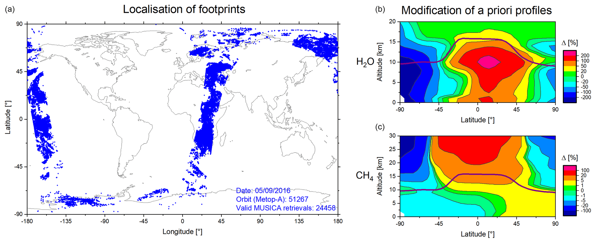
Figure B1Setup of the linearity test using modified a priori data. (a) The localisation of the footprints of the exemplary orbit used and (b, c) latitudinal cross sections documenting the modification of the H2O and CH4 a priori data (modified − original; the thick solid violet line indicates the tropopause altitude).

Figure B2Results of the individually performed linearity tests for H2O and CH4. Shown are the following three latitudinal cross sections: (1) rms values between the original retrieval (retrieval results using the original a priori data) and the modified retrieval (retrieval results using the modified a priori data), (2) rms values between the modified retrieval and the original retrieval after performing the a posteriori adjustment according to Eq. (B1) on a logarithmic scale, and (3) same as (2) but for the a posteriori adjustment performed on a linear scale. The thick solid violet line indicates the tropopause altitude.
The linearity test consists in comparing the results obtained by the full retrieval using the modified a priori data and the results obtained by using the analytic treatment according to Eq. (B1).
B2 Test results for logarithmic and linear scale
The results of the linearity test are shown in Fig. B2. We demonstrate the impact of the modified a priori by calculating the differences between the original retrieval and the additional retrieval using the modified a priori profiles. We make a latitudinally dependent characterisation of these differences by calculating root-mean-square (rms) values of the differences within 5∘ latitude bands. Latitudinal cross sections of these rms differences are depicted on the left of Fig. B2 and reveal that the impact of the modified a priori on the retrieval is largest at the winter polar regions (high southern latitudes). This is where we find large differences between the original and the modified a priori (see Fig. B1) and where at the same time the retrieval sensitivity is relatively low (see DOFS maps in Fig. 10).
The centre and right columns of Fig. B2 show the 5∘ latitude band rms values for differences between the additional retrieval using the modified a priori profiles and the modification according to the analytic calculations of Eq. (B1). The centre column shows the results when performing the calculations of Eq. (B1) on the logarithmic scale. We observe that with the analytic calculations we can almost achieve the same results as with the full retrieval calculations. This indicates that the assumption of linearity for such analytic calculation is indeed valid. The right column shows the results when performing the calculations of Eq. (B1) on the linear scale; i.e. state vectors as well as derivatives (here the averaging kernel entries) are used on the linear scale (). The linearity assumption is not valid when performing the analytic calculation for H2O on the linear scale. We see very large differences between the full retrieval results and the results obtained by Eq. (B1). For CH4 the linear-scale analytic calculations have worse agreement with the full retrievals than the logarithmic-scale calculations; however, they are not that pronounced as in the case of H2O. The reason for this is the setup of the linearity test (see Fig. B1 and the corresponding discussion): for the test the modification of the CH4 a priori is weak, but for H2O the a priori modification is rather strong.
In summary, the test shows that the assumption of linearity needed for an analytic treatment of the MUSICA IASI trace gas data is valid. Nevertheless, we have to be careful. Because the retrievals are performed in the logarithmic scale, the analytic calculation that uses the averaging kernels, gain matrices, or constraint matrices should also be performed on the logarithmic scale. On this scale the linearity assumption is valid, which is contrary to the linear scale, where the linearity assumption is not valid, meaning that an analytic treatment on the linear scale can lead to large errors.
For converting mixing ratio profiles into amount profiles we set up a pressure weighting operator Z as a diagonal matrix with the following entries:
Using the pressure pi at atmospheric grid level i we use , , and for . Furthermore, gi is the gravitational acceleration at level i; mair and the molecular mass of dry air and water vapour, respectively; and the retrieved water vapour mixing ratio at level i.
We define an operator WT for resampling fine gridded atmospheric amount profiles into coarse gridded atmospheric partial column amount profiles. It has the dimension c×nal, where c is the number of the resampled coarse atmospheric grid levels and nal the number of atmospheric levels of the original fine atmospheric grid. Each line of the operator has the value 1 for the levels that are resampled and 0 for all other levels:
We can combine the operators Z and WT and calculate a pressure-weighted resampling operator by
This operator resamples linear-scale mixing ratio profiles into linear-scale partial column-averaged mixing ratio profiles.
With operator we can calculate a coarse gridded partial column-averaged state from the fine gridded linear mixing ratio state by
Furthermore, we introduce an operator L for transferring the differentials from the logarithmic mixing ratio scale to differentials in linear mixing ratio scale. It is a diagonal matrix having the elements of the linear-scale atmospheric mixing ratios' state as the diagonal elements:
The averaging kernel of the partial column-averaged state can be calculated from the averaging kernel of the fine gridded logarithmic scale (A) by
This kernel describes how a change in the partial column-averaged mixing ratios affects the retrieved partial column-averaged mixing ratios. This is an approximation because on the right side the diagonal values of L should be the actual mixing ratios instead of those retrieved. The matrix W is an interpolation matrix that resamples the coarse gridded partial column-averaged mixing ratio profiles as a fine gridded mixing ratio profile without modifying the partial columns. It is , which can be easily seen by using from Eq. (C3).
The covariances of the partial column-averaged mixing ratio state can be calculated from the corresponding covariance matrices of the fine gridded logarithmic scale (S) by
Here the approximation is because Δx≈xΔln x.
MS set up the MUSICA IASI retrieval, designed the netCDF CF conform MUSICA IASI output files, made the calculations in the context of the extended output file, developed and performed the compression of the averaging kernel output, and wrote this paper. BE developed the efficient MUSICA IASI processing chain and ran the processing at the supercomputer ForHLR. CJD supported the paper with several graphics. FK, CJD, and BE helped in preparing the MUSICA IASI output files with the compressed averaging kernels. AW developed the software tool for compressing the averaging kernels. FH developed the PROFFIT-nadir retrieval code. MH provided the code use for the MT_CKD water continuum calculations and helped with the scattering calculation needed for the cloud spectral responses. OEG and ES provided the MUSICA IASI processed data product generated at the Teide supercomputer. DK provided the CESM1–WACCM data used for generating the MUSICA IASI trace gas a priori data. All authors contributed with corrections and comments to the final version of the manuscript.
The contact author has declared that neither they nor their co-authors have any competing interests.
Publisher’s note: Copernicus Publications remains neutral with regard to jurisdictional claims in published maps and institutional affiliations.
This work has strongly benefited from the project MUSICA (funded by the European Research Council under the European Community's Seventh Framework Programme (FP7/2007-2013), ERC grant agreement number 256961), from financial support in the context of the projects MOTIV and TEDDY (funded by the Deutsche Forschungsgemeinschaft under project IDs [Geschäftszeichen] 290612604/GZ:SCHN1126/2-1 and 416767181/GZ:SCHN1126/5-1, respectively), and from INMENSE (funded by the Ministerio de Economía y Competividad from Spain, CGL2016-80688-P).
Retrieval calculations for this work were performed on the supercomputer ForHLR funded by the Ministry of Science, Research and the Arts Baden-Württemberg and by the German Federal Ministry of Education and Research. Furthermore, we acknowledge the contribution of Teide High Performance Computing (TeideHPC) facilities. TeideHPC facilities are provided by the Instituto Tecnológico y de Energías Renovables (ITER), S.A (https://teidehpc.iter.es, last access: 25 January 2022).
This research has been supported by the European Research Council, FP7 Ideas (MUSICA (grant no. 256961)); the Deutsche Forschungsgemeinschaft (grant nos. 290612604, project MOTIV, and 416767181, project TEDDY); the Ministerio de Economía y Competitividad (grant no. CGL2016-80688-P, project INMENSE); the Bundesministerium für Bildung und Forschung (ForHLR supercomputer); and the Ministerium für Wissenschaft, Forschung und Kunst Baden-Württemberg (ForHLR supercomputer).
This paper was edited by Nellie Elguindi and reviewed by Leonid Yurganov and one anonymous referee.
August, T., Klaes, D., Schluessel, P., Hultberg, T., Crapeau, M., Arriaga, A., O'Carroll, A., Coppens, D., Munro, R., and Calbet, X.: IASI on Metop-A: Operational Level 2 retrievals after five years in orbit, J. Quant. Spectrosc. Ra., 113, 1340–1371, https://doi.org/10.1016/j.jqsrt.2012.02.028, 2012. a, b, c, d
Backus, G. E. and Gilbert, F.: Uniqueness in the Inversion of inaccurate Gross Earth Data, Philos. T. R. Soc. A, 266, 123–192, 1970. a
Baldridge, A., Hook, S., Grove, C., and Rivera, G.: The ASTER spectral library version 2.0, Remote Sens. Environ., 113, 711–715, https://doi.org/10.1016/j.rse.2008.11.007, 2009. a
Baron, P., Ricaud, P., de la Noë, J., Eriksson, J. E., Merino, F., Ridal, M., and Murtagh, D. P.: Studies for the Odin sub-millimetre radiometer. II. Retrieval methodology, Can. J. Phys., 80, 341–356, https://doi.org/10.1139/p01-150, 2002. a
Barthlott, S., Schneider, M., Hase, F., Wiegele, A., Christner, E., González, Y., Blumenstock, T., Dohe, S., García, O. E., Sepúlveda, E., Strong, K., Mendonca, J., Weaver, D., Palm, M., Deutscher, N. M., Warneke, T., Notholt, J., Lejeune, B., Mahieu, E., Jones, N., Griffith, D. W. T., Velazco, V. A., Smale, D., Robinson, J., Kivi, R., Heikkinen, P., and Raffalski, U.: Using XCO2 retrievals for assessing the long-term consistency of NDACC/FTIR data sets, Atmos. Meas. Tech., 8, 1555–1573, https://doi.org/10.5194/amt-8-1555-2015, 2015. a
Barthlott, S., Schneider, M., Hase, F., Blumenstock, T., Kiel, M., Dubravica, D., García, O. E., Sepúlveda, E., Mengistu Tsidu, G., Takele Kenea, S., Grutter, M., Plaza-Medina, E. F., Stremme, W., Strong, K., Weaver, D., Palm, M., Warneke, T., Notholt, J., Mahieu, E., Servais, C., Jones, N., Griffith, D. W. T., Smale, D., and Robinson, J.: Tropospheric water vapour isotopologue data (, , and HD16O) as obtained from NDACC/FTIR solar absorption spectra, Earth Syst. Sci. Data, 9, 15–29, https://doi.org/10.5194/essd-9-15-2017, 2017. a
Blumstein, D., Chalon, G., Carlier, T., Buil, C., Hebert, P., Maciaszek, T., Ponce, G., Phulpin, T., Tournier, B., Simeoni, D., Astruc, P., Clauss, A., Kayal, G., and Jegou, R.: IASI instrument: technical overview and measured performances, in: Infrared Spaceborne Remote Sensing XII, edited by: Strojnik, M., vol. 5543, International Society for Optics and Photonics, SPIE, 196–207, https://doi.org/10.1117/12.560907, 2004. a
Borger, C., Schneider, M., Ertl, B., Hase, F., García, O. E., Sommer, M., Höpfner, M., Tjemkes, S. A., and Calbet, X.: Evaluation of MUSICA IASI tropospheric water vapour profiles using theoretical error assessments and comparisons to GRUAN Vaisala RS92 measurements, Atmos. Meas. Tech., 11, 4981–5006, https://doi.org/10.5194/amt-11-4981-2018, 2018. a, b, c
Boynard, A., Hurtmans, D., Garane, K., Goutail, F., Hadji-Lazaro, J., Koukouli, M. E., Wespes, C., Vigouroux, C., Keppens, A., Pommereau, J.-P., Pazmino, A., Balis, D., Loyola, D., Valks, P., Sussmann, R., Smale, D., Coheur, P.-F., and Clerbaux, C.: Validation of the IASI FORLI/EUMETSAT ozone products using satellite (GOME-2), ground-based (Brewer–Dobson, SAOZ, FTIR) and ozonesonde measurements, Atmos. Meas. Tech., 11, 5125–5152, https://doi.org/10.5194/amt-11-5125-2018, 2018. a
Christner, E., Aemisegger, F., Pfahl, S., Werner, M., Cauquoin, A., Schneider, M., Hase, F., Barthlott, S., and Schädler, G.: The Climatological Impacts of Continental Surface Evaporation, Rainout, and Subcloud Processes on δD of Water Vapor and Precipitation in Europe, J. Geophys. Res.-Atmos., 123, 4390–4409, https://doi.org/10.1002/2017JD027260, 2018. a
Clerbaux, C., Boynard, A., Clarisse, L., George, M., Hadji-Lazaro, J., Herbin, H., Hurtmans, D., Pommier, M., Razavi, A., Turquety, S., Wespes, C., and Coheur, P.-F.: Monitoring of atmospheric composition using the thermal infrared IASI/MetOp sounder, Atmos. Chem. Phys., 9, 6041–6054, https://doi.org/10.5194/acp-9-6041-2009, 2009. a, b
Delamere, J. S., Clough, S. A., Payne, V. H., Mlawer, E. J., Turner, D. D., and Gamache, R. R.: A far-infrared radiative closure study in the Arctic: Application to water vapor, J. Geophys. Res.-Atmos., 115, D17106, https://doi.org/10.1029/2009JD012968, 2010. a, b
De Wachter, E., Barret, B., Le Flochmoën, E., Pavelin, E., Matricardi, M., Clerbaux, C., Hadji-Lazaro, J., George, M., Hurtmans, D., Coheur, P.-F., Nedelec, P., and Cammas, J. P.: Retrieval of MetOp-A/IASI CO profiles and validation with MOZAIC data, Atmos. Meas. Tech., 5, 2843–2857, https://doi.org/10.5194/amt-5-2843-2012, 2012. a
De Wachter, E., Kumps, N., Vandaele, A. C., Langerock, B., and De Mazière, M.: Retrieval and validation of MetOp/IASI methane, Atmos. Meas. Tech., 10, 4623–4638, https://doi.org/10.5194/amt-10-4623-2017, 2017. a
Diekmann, C. J., Schneider, M., Ertl, B., Hase, F., García, O., Khosrawi, F., Sepúlveda, E., Knippertz, P., and Braesicke, P.: The global and multi-annual MUSICA IASI {H2O, δD} pair dataset, Earth Syst. Sci. Data, 13, 5273–5292, https://doi.org/10.5194/essd-13-5273-2021, 2021. a, b, c, d, e
Dirksen, R. J., Sommer, M., Immler, F. J., Hurst, D. F., Kivi, R., and Vömel, H.: Reference quality upper-air measurements: GRUAN data processing for the Vaisala RS92 radiosonde, Atmos. Meas. Tech., 7, 4463–4490, https://doi.org/10.5194/amt-7-4463-2014, 2014. a
Dyroff, C., Sanati, S., Christner, E., Zahn, A., Balzer, M., Bouquet, H., McManus, J. B., González-Ramos, Y., and Schneider, M.: Airborne in situ vertical profiling of HDO in the subtropical troposphere during the MUSICA remote sensing validation campaign, Atmos. Meas. Tech., 8, 2037–2049, https://doi.org/10.5194/amt-8-2037-2015, 2015. a, b
Eriksson, P.: Analysis and comparison of two linear regularization methods for passive atmospheric observations, J. Geophys. Res.-Atmos., 105, 18157–18167, https://doi.org/10.1029/2000JD900172, 2000. a
Franco, B., Clarisse, L., Stavrakou, T., Müller, J.-F., Van Damme, M., Whitburn, S., Hadji-Lazaro, J., Hurtmans, D., Taraborrelli, D., Clerbaux, C., and Coheur, P.-F.: A General Framework for Global Retrievals of Trace Gases From IASI: Application to Methanol, Formic Acid, and PAN, J. Geophys. Res.-Atmos., 123, 13963–13984, https://doi.org/10.1029/2018JD029633, 2018. a
Gamache, R. R., Lamouroux, J., Blot-Lafon, V., and Lopes, E.: An intercomparison of measured pressure-broadening, pressure shifting parameters of carbon dioxide and their temperature dependence, J. Quant. Spectrosc. Ra., 135, 30–43, https://doi.org/10.1016/j.jqsrt.2013.11.001, 2014. a
García, O. E., Schneider, M., Ertl, B., Sepúlveda, E., Borger, C., Diekmann, C., Wiegele, A., Hase, F., Barthlott, S., Blumenstock, T., Raffalski, U., Gómez-Peláez, A., Steinbacher, M., Ries, L., and de Frutos, A. M.: The MUSICA IASI CH4 and N2O products and their comparison to HIPPO, GAW and NDACC FTIR references, Atmos. Meas. Tech., 11, 4171–4215, https://doi.org/10.5194/amt-11-4171-2018, 2018. a, b, c, d, e, f
Gomez-Pelaez, A. J., Ramos, R., Cuevas, E., Gomez-Trueba, V., and Reyes, E.: Atmospheric CO2, CH4, and CO with the CRDS technique at the Izaña Global GAW station: instrumental tests, developments, and first measurement results, Atmos. Meas. Tech., 12, 2043–2066, https://doi.org/10.5194/amt-12-2043-2019, 2019. a
González, Y., Schneider, M., Dyroff, C., Rodríguez, S., Christner, E., García, O. E., Cuevas, E., Bustos, J. J., Ramos, R., Guirado-Fuentes, C., Barthlott, S., Wiegele, A., and Sepúlveda, E.: Detecting moisture transport pathways to the subtropical North Atlantic free troposphere using paired H2O-δD in situ measurements, Atmos. Chem. Phys., 16, 4251–4269, https://doi.org/10.5194/acp-16-4251-2016, 2016. a, b
Gordon, I., Rothman, L., Hill, C., Kochanov, R., Tan, Y., Bernath, P., Birk, M., Boudon, V., Campargue, A., Chance, K., Drouin, B., Flaud, J.-M., Gamache, R., Hodges, J., Jacquemart, D., Perevalov, V., Perrin, A., Shine, K., Smith, M.-A., Tennyson, J., Toon, G., Tran, H., Tyuterev, V., Barbe, A., Császár, A., Devi, V., Furtenbacher, T., Harrison, J., Hartmann, J.-M., Jolly, A., Johnson, T., Karman, T., Kleiner, I., Kyuberis, A., Loos, J., Lyulin, O., Massie, S., Mikhailenko, S., Moazzen-Ahmadi, N., Müller, H., Naumenko, O., Nikitin, A., Polyansky, O., Rey, M., Rotger, M., Sharpe, S., Sung, K., Starikova, E., Tashkun, S., Auwera, J. V., Wagner, G., Wilzewski, J., Wcisło, P., Yu, S., and Zak, E.: The HITRAN2016 molecular spectroscopic database, J. Quant. Spectrosc. Ra., 203, 3–69, https://doi.org/10.1016/j.jqsrt.2017.06.038, 2017. a, b, c
Hase, F., Hannigan, J. W., Coffey, M. T., Goldman, A., Höpfner, M., Jones, N. B., Rinsland, C. P., and Wood, S.: Intercomparison of retrieval codes used for the analysis of high-resolution, J. Quant. Spectrosc. Ra., 87, 25–52, 2004. a, b, c
Hess, M., Koepke, P., and Schult, I.: Optical Properties of Aerosols and Clouds: The Software Package OPAC, B. Am. Meteorol. Soc., 79, 831–844, https://doi.org/10.1175/1520-0477(1998)079<0831:OPOAAC>2.0.CO;2, 1998. a, b, c, d, e
Kalman, R. E.: A new approach to linear filtering and prediction problems, J. Basic Eng., 82, 35–45, https://doi.org/10.1115/1.3662552, 1960. a
Karion, A., Sweeney, C., Tans, P., and Newberger, T.: AirCore: An Innovative Atmospheric Sampling System, J. Atmos. Ocean. Tech., 27, 1839–1853, https://doi.org/10.1175/2010JTECHA1448.1, 2010. a
Keim, C., Eremenko, M., Orphal, J., Dufour, G., Flaud, J.-M., Höpfner, M., Boynard, A., Clerbaux, C., Payan, S., Coheur, P.-F., Hurtmans, D., Claude, H., Dier, H., Johnson, B., Kelder, H., Kivi, R., Koide, T., López Bartolomé, M., Lambkin, K., Moore, D., Schmidlin, F. J., and Stübi, R.: Tropospheric ozone from IASI: comparison of different inversion algorithms and validation with ozone sondes in the northern middle latitudes, Atmos. Chem. Phys., 9, 9329–9347, https://doi.org/10.5194/acp-9-9329-2009, 2009. a
Keppens, A., Lambert, J.-C., Granville, J., Miles, G., Siddans, R., van Peet, J. C. A., van der A, R. J., Hubert, D., Verhoelst, T., Delcloo, A., Godin-Beekmann, S., Kivi, R., Stübi, R., and Zehner, C.: Round-robin evaluation of nadir ozone profile retrievals: methodology and application to MetOp-A GOME-2, Atmos. Meas. Tech., 8, 2093–2120, https://doi.org/10.5194/amt-8-2093-2015, 2015. a, b, c
Koepke, P., Gasteiger, J., and Hess, M.: Technical Note: Optical properties of desert aerosol with non-spherical mineral particles: data incorporated to OPAC, Atmos. Chem. Phys., 15, 5947–5956, https://doi.org/10.5194/acp-15-5947-2015, 2015. a
Kohlhepp, R., Ruhnke, R., Chipperfield, M. P., De Mazière, M., Notholt, J., Barthlott, S., Batchelor, R. L., Blatherwick, R. D., Blumenstock, Th., Coffey, M. T., Demoulin, P., Fast, H., Feng, W., Goldman, A., Griffith, D. W. T., Hamann, K., Hannigan, J. W., Hase, F., Jones, N. B., Kagawa, A., Kaiser, I., Kasai, Y., Kirner, O., Kouker, W., Lindenmaier, R., Mahieu, E., Mittermeier, R. L., Monge-Sanz, B., Morino, I., Murata, I., Nakajima, H., Palm, M., Paton-Walsh, C., Raffalski, U., Reddmann, Th., Rettinger, M., Rinsland, C. P., Rozanov, E., Schneider, M., Senten, C., Servais, C., Sinnhuber, B.-M., Smale, D., Strong, K., Sussmann, R., Taylor, J. R., Vanhaelewyn, G., Warneke, T., Whaley, C., Wiehle, M., and Wood, S. W.: Observed and simulated time evolution of HCl, ClONO2, and HF total column abundances, Atmos. Chem. Phys., 12, 3527–3556, https://doi.org/10.5194/acp-12-3527-2012, 2012. a
Kunz, A., Pan, L. L., Konopka, P., Kinnison, D. E., and Tilmes, S.: Chemical and dynamical discontinuity at the extratropical tropopause based on START08 and WACCM analyses, J. Geophys. Res.-Atmos., 116, D24302, https://doi.org/10.1029/2011JD016686, 2011. a
Lacour, J.-L., Risi, C., Clarisse, L., Bony, S., Hurtmans, D., Clerbaux, C., and Coheur, P.-F.: Mid-tropospheric δD observations from IASI/MetOp at high spatial and temporal resolution, Atmos. Chem. Phys., 12, 10817–10832, https://doi.org/10.5194/acp-12-10817-2012, 2012. a, b
Lorente, A., Borsdorff, T., Butz, A., Hasekamp, O., aan de Brugh, J., Schneider, A., Wu, L., Hase, F., Kivi, R., Wunch, D., Pollard, D. F., Shiomi, K., Deutscher, N. M., Velazco, V. A., Roehl, C. M., Wennberg, P. O., Warneke, T., and Landgraf, J.: Methane retrieved from TROPOMI: improvement of the data product and validation of the first 2 years of measurements, Atmos. Meas. Tech., 14, 665–684, https://doi.org/10.5194/amt-14-665-2021, 2021. a
Marsh, D. R., Mills, M. J., Kinnison, D. E., Lamarque, J.-F., Calvo, N., and Polvani, L. M.: Climate Change from 1850 to 2005 Simulated in CESM1(WACCM), J. Climate, 26, 7372–7391, https://doi.org/10.1175/JCLI-D-12-00558.1, 2013. a
Masuda, K., Takashima, T., and Takayama, Y.: Emissivity of pure and sea waters for the model sea surface in the infrared window regions, Remote Sens. Environ., 24, 313–329, https://doi.org/10.1016/0034-4257(88)90032-6, 1988. a, b, c
Mlawer, E. J., Payne, V. H., Moncet, J.-L., Delamere, J. S., Alvarado, M. J., and Tobin, D. C.: Development and recent evaluation of the MT_CKD model of continuum absorption, Philos. T. R. Soc. A, 370, 2520–2556, https://doi.org/10.1098/rsta.2011.0295, 2012. a, b
Morgenstern, O., Hegglin, M. I., Rozanov, E., O'Connor, F. M., Abraham, N. L., Akiyoshi, H., Archibald, A. T., Bekki, S., Butchart, N., Chipperfield, M. P., Deushi, M., Dhomse, S. S., Garcia, R. R., Hardiman, S. C., Horowitz, L. W., Jöckel, P., Josse, B., Kinnison, D., Lin, M., Mancini, E., Manyin, M. E., Marchand, M., Marécal, V., Michou, M., Oman, L. D., Pitari, G., Plummer, D. A., Revell, L. E., Saint-Martin, D., Schofield, R., Stenke, A., Stone, K., Sudo, K., Tanaka, T. Y., Tilmes, S., Yamashita, Y., Yoshida, K., and Zeng, G.: Review of the global models used within phase 1 of the Chemistry–Climate Model Initiative (CCMI), Geosci. Model Dev., 10, 639–671, https://doi.org/10.5194/gmd-10-639-2017, 2017. a
Payne, V. H., Mlawer, E. J., Cady-Pereira, K. E., and Moncet, J. L.: Water Vapor Continuum Absorption in the Microwave, IEEE T. Geosci. Remote, 49, 2194–2208, https://doi.org/10.1109/TGRS.2010.2091416, 2011. a, b
Purser, R. J. and Huang, H.-L.: Estimating Effective Data Density in a Satellite Retrieval or an Objective Analysis, J. Appl. Meteorol., 32, 1092–1107, https://doi.org/10.1175/1520-0450(1993)032<1092:EEDDIA>2.0.CO;2, 1993. a
Rienecker, M. M., Suarez, M. J., Gelaro, R., Todling, R., Bacmeister, J., Liu, E., Bosilovich, M. G., Schubert, S. D., Takacs, L., Kim, G.-K., Bloom, S., Chen, J., Collins, D., Conaty, A., da Silva, A., Gu, W., Joiner, J., Koster, R. D., Lucchesi, R., Molod, A., Owens, T., Pawson, S., Pegion, P., Redder, C. R., Reichle, R., Robertson, F. R., Ruddick, A. G., Sienkiewicz, M., and Woollen, J.: MERRA: NASA’s Modern-Era Retrospective Analysis for Research and Applications, J. Climate, 24, 3624–3648, https://doi.org/10.1175/JCLI-D-11-00015.1, 2011. a
Risi, C., Bony, S., Vimeux, F., and Jouzel, J.: Water-stable isotopes in the LMDZ4 general circulation model: Model evaluation for present-day and past climates and applications to climatic interpretations of tropical isotopic records, Journal of Geophysical Research: Atmospheres, 115, https://doi.org/10.1029/2009JD013255, 2010. a
Rodgers, C.: Inverse Methods for Atmospheric Sounding: Theory and Praxis, Series on Atmospheric, Oceanic and Planetary Physics – Vol. 2, edited by: Taylor, F. W. (University of Oxford), World Scientific Publishing Co., Singapore, ISBN 981-02-2740-X, 2000. a, b, c, d, e, f, g, h, i
Rodgers, C. and Connor, B.: Intercomparison of remote sounding instruments, J. Geophys. Res., 108, 4116–4129, https://doi.org/10.1029/2002JD002299, 2003. a
Ronsmans, G., Langerock, B., Wespes, C., Hannigan, J. W., Hase, F., Kerzenmacher, T., Mahieu, E., Schneider, M., Smale, D., Hurtmans, D., De Mazière, M., Clerbaux, C., and Coheur, P.-F.: First characterization and validation of FORLI-HNO3 vertical profiles retrieved from IASI/Metop, Atmos. Meas. Tech., 9, 4783–4801, https://doi.org/10.5194/amt-9-4783-2016, 2016. a
Schneider, M. and Hase, F.: Improving spectroscopic line parameters by means of atmospheric spectra: Theory and example for water vapour and solar absorption spectra, J. Quant. Spectrosc. Ra., 110, 1825–1839, https://doi.org/10.1016/j.jqsrt.2009.04.011, 2009. a
Schneider, M. and Hase, F.: Optimal estimation of tropospheric H2O and δD with IASI/METOP, Atmos. Chem. Phys., 11, 11207–11220, https://doi.org/10.5194/acp-11-11207-2011, 2011. a, b
Schneider, M., Hase, F., and Blumenstock, T.: Water vapour profiles by ground-based FTIR spectroscopy: study for an optimised retrieval and its validation, Atmos. Chem. Phys., 6, 811–830, https://doi.org/10.5194/acp-6-811-2006, 2006a. a
Schneider, M., Hase, F., and Blumenstock, T.: Ground-based remote sensing of ratio profiles: introduction and validation of an innovative retrieval approach, Atmos. Chem. Phys., 6, 4705–4722, https://doi.org/10.5194/acp-6-4705-2006, 2006b. a
Schneider, M., Barthlott, S., Hase, F., González, Y., Yoshimura, K., García, O. E., Sepúlveda, E., Gomez-Pelaez, A., Gisi, M., Kohlhepp, R., Dohe, S., Blumenstock, T., Wiegele, A., Christner, E., Strong, K., Weaver, D., Palm, M., Deutscher, N. M., Warneke, T., Notholt, J., Lejeune, B., Demoulin, P., Jones, N., Griffith, D. W. T., Smale, D., and Robinson, J.: Ground-based remote sensing of tropospheric water vapour isotopologues within the project MUSICA, Atmos. Meas. Tech., 5, 3007–3027, https://doi.org/10.5194/amt-5-3007-2012, 2012. a, b, c
Schneider, M., González, Y., Dyroff, C., Christner, E., Wiegele, A., Barthlott, S., García, O. E., Sepúlveda, E., Hase, F., Andrey, J., Blumenstock, T., Guirado, C., Ramos, R., and Rodríguez, S.: Empirical validation and proof of added value of MUSICA's tropospheric δD remote sensing products, Atmos. Meas. Tech., 8, 483–503, https://doi.org/10.5194/amt-8-483-2015, 2015. a
Schneider, M., Ertl, B., and Diekmann, C.: MUSICA IASI full retrieval product extended output (processing version 3.2.1), KIT [data set], https://doi.org/10.35097/412, 2021a. a, b, c
Schneider, M., Ertl, B., and Diekmann, C.: MUSICA IASI full retrieval product standard output (processing version 3.2.1), KIT [data set], https://doi.org/10.35097/408, 2021b. a, b, c
Schneider, M., Ertl, B., Diekmann, C. J., Khosrawi, F., Röhling, A. N., Hase, F., Dubravica, D., García, O. E., Sepúlveda, E., Borsdorff, T., Landgraf, J., Lorente, A., Chen, H., Kivi, R., Laemmel, T., Ramonet, M., Crevoisier, C., Pernin, J., Steinbacher, M., Meinhardt, F., Deutscher, N. M., Griffith, D. W. T., Velazco, V. A., and Pollard, D. F.: Synergetic use of IASI and TROPOMI space borne sensors for generating a tropospheric methane profile product, Atmos. Meas. Tech. Discuss. [preprint], https://doi.org/10.5194/amt-2021-31, in review, 2021c. a, b
Seemann, S. W., Borbas, E. E., Knuteson, R. O., Stephenson, G. R., and Huang, H.-L.: Development of a Global Infrared Land Surface Emissivity Database for Application to Clear Sky Sounding Retrievals from Multispectral Satellite Radiance Measurements, J. Appl. Meteorol. Clim., 47, 108–123, https://doi.org/10.1175/2007JAMC1590.1, 2008. a, b, c, d
Siddans, R., Knappett, D., Kerridge, B., Waterfall, A., Hurley, J., Latter, B., Boesch, H., and Parker, R.: Global height-resolved methane retrievals from the Infrared Atmospheric Sounding Interferometer (IASI) on MetOp, Atmos. Meas. Tech., 10, 4135–4164, https://doi.org/10.5194/amt-10-4135-2017, 2017. a
Steck, T.: Methods for determining regularization for atmospheric retrieval problems, Appl. Opt., 41, 1788–1797, https://doi.org/10.1364/AO.41.001788, 2002. a
Stiller, G. P. (Ed.): The Karlsruhe Optimized and Precise Radiative transfer Algorithm (KOPRA), Vol. FZKA 6487 of Wissenschaftliche Berichte, Forschungszentrum Karlsruhe, 2000. a
Tikhonov, A. N.: Solution of Incorrectly Formulated Problems and the Regularization Method, Soviet Mathematics Doklady, 4, 1035–1038, 1963. a
von Clarmann, T., Degenstein, D. A., Livesey, N. J., Bender, S., Braverman, A., Butz, A., Compernolle, S., Damadeo, R., Dueck, S., Eriksson, P., Funke, B., Johnson, M. C., Kasai, Y., Keppens, A., Kleinert, A., Kramarova, N. A., Laeng, A., Langerock, B., Payne, V. H., Rozanov, A., Sato, T. O., Schneider, M., Sheese, P., Sofieva, V., Stiller, G. P., von Savigny, C., and Zawada, D.: Overview: Estimating and reporting uncertainties in remotely sensed atmospheric composition and temperature, Atmos. Meas. Tech., 13, 4393–4436, https://doi.org/10.5194/amt-13-4393-2020, 2020. a
Weber, A.: Storage-Efficient Analysis of Spatio-Temporal Data with Application to Climate Research, Master Thesis, Karlsruhe Institute of Technology, https://doi.org/10.5281/ZENODO.3360021, 2019. a, b
Wiegele, A., Schneider, M., Hase, F., Barthlott, S., García, O. E., Sepúlveda, E., González, Y., Blumenstock, T., Raffalski, U., Gisi, M., and Kohlhepp, R.: The MUSICA MetOp/IASI H2O and δD products: characterisation and long-term comparison to NDACC/FTIR data, Atmos. Meas. Tech., 7, 2719–2732, https://doi.org/10.5194/amt-7-2719-2014, 2014. a
Wilkinson, M. D., Dumontier, M., Aalbersberg, I. J., Appleton, G., Axton, M., Baak, A., Blomberg, N., Boiten, J.-W., da Silva Santos, L. B., Bourne, P. E., Bouwman, J., Brookes, A. J., Clark, T., Crosas, M., Dillo, I., Dumon, O., Edmunds, S., Evelo, C. T., Finkers, R., Gonzalez-Beltran, A., Gray, A. J., Groth, P., Goble, C., Grethe, J. S., Heringa, J., 't Hoen, P. A., Hooft, R., Kuhn, T., Kok, R., Kok, J., Lusher, S. J., Martone, M. E., Mons, A., Packer, A. L., Persson, B., Rocca-Serra, P., Roos, M., van Schaik, R., Sansone, S.-A., Schultes, E., Sengstag, T., Slater, T., Strawn, G., Swertz, M. A., Thompson, M., van der Lei, J., van Mulligen, E., Velterop, J., Waagmeester, A., Wittenburg, P., Wolstencroft, K., Zhao, J., and Mons, B.: The FAIR Guiding Principles for scientific data management and stewardship, Sci Data, 3, 2052–4463, https://doi.org/10.1038/sdata.2016.18, 2016. a
Wofsy, S. C.: HIAPER Pole-to-Pole Observations (HIPPO): fine-grained, global-scale measurements of climatically important atmospheric gases and aerosols, Philos. T. R. Soc. A, 369, 2073–2086, https://doi.org/10.1098/rsta.2010.0313, 2011. a
Worden, J., Kulawik, S., Frankenberg, C., Payne, V., Bowman, K., Cady-Peirara, K., Wecht, K., Lee, J.-E., and Noone, D.: Profiles of CH4, HDO, H2O, and N2O with improved lower tropospheric vertical resolution from Aura TES radiances, Atmos. Meas. Tech., 5, 397–411, https://doi.org/10.5194/amt-5-397-2012, 2012. a
- Abstract
- Introduction
- The IASI instruments on Metop satellites
- MUSICA IASI data format
- MUSICA IASI retrieval setup
- MUSICA IASI retrieval output
- Data filtering options
- Data examples
- Interoperability and data reusage
- Data availability
- Summary and outlook
- Appendix A: Basics of retrieval theory and notations
- Appendix B: Linearity
- Appendix C: Partial column-averaged mixing ratios
- Author contributions
- Competing interests
- Disclaimer
- Acknowledgements
- Financial support
- Review statement
- References