the Creative Commons Attribution 4.0 License.
the Creative Commons Attribution 4.0 License.
 | 17 Feb 2022
Rainfall erosivity mapping over mainland China based on high-density hourly rainfall records
Tianyu Yue
Shuiqing Yin
Yun Xie
Bofu Yu
Baoyuan Liu
Rainfall erosivity quantifies the effect of rainfall and runoff on the rate of soil loss. Maps of rainfall erosivity are needed for erosion assessment using the Universal Soil Loss Equation (USLE) and its successors. To improve erosivity maps that are currently available, hourly and daily rainfall data from 2381 stations for the period 1951–2018 were used to generate new R-factor and 1-in-10-year event EI30 maps for mainland China (available at https://doi.org/10.12275/bnu.clicia.rainfallerosivity.CN.001; Yue et al., 2020b). One-minute rainfall data from 62 stations, of which 18 had a record length > 29 years, were used to compute the “true” rainfall erosivity against which the new R-factor and 1-in-10-year EI30 maps were assessed to quantify the improvement over the existing maps through cross-validation. The results showed that (1) existing maps underestimated erosivity for most of the south-eastern part of China and overestimated for most of the western region; (2) the new R-factor map generated in this study had a median absolute relative error of 16 % for the western region, compared to 162 % for the existing map, and 18 % for the rest of China. The new 1-in-10-year EI30 map had a median absolute relative error of 14 % for the central and eastern regions of China, compared to 21 % for the existing map (map accuracy was not evaluated for the western region where the 1 min data were limited); (3) the R-factor map was improved mainly for the western region, because of an increase in the number of stations from 87 to 150 and temporal resolution from daily to hourly; (4) the benefit of increased station density for erosivity mapping is limited once the station density reached about 1 station per 10 000 km2.
- Article
(8620 KB) - Full-text XML
- BibTeX
- EndNote


Soil erosion has been a major threat to soil health, soil and river ecosystem services in many regions of the world (Pennock, 2019). Soil erosion has on-site impacts, such as the reduction of soil and water, the loss of soil nutrients, the decrease of land quality and food production, as well as off-site impacts, such as excessive sedimentation and water pollution.
Soil erosion models are tools to evaluate the rate of soil loss and can provide policymakers useful information for taking measures in soil and water conservation. The Universal Soil Loss Equation (USLE; Wischmeier and Smith, 1965, 1978) and the Revised USLE (RUSLE; Renard et al., 1997; USDA-ARS, 2013) have been widely used to estimate soil erosion in at least 109 countries over the past 40 years (Alewell et al., 2019). Rainfall erosivity is one of the factors in the USLE and RUSLE to represent the potential ability of rainfall and runoff to affect soil erosion.
In the USLE, erosivity of a rainfall event is identified as the EI value, also denoted as EI30, which is the product of the total storm energy (E) and the maximum 30 min intensity (I30) (Wischmeier, 1959). The erosivity factor (R-factor) in the USLE is the mean annual total EI values of all erosive events. To recognize interannual rainfall variability, rainfall data of long periods are required (Wischmeier and Smith, 1978). In the original isoerodent maps generated by Wischmeier and Smith (1965), stations with rainfall data of at least 22 years were used.
To use the USLE, two additional input parameters are required. One is the seasonal distribution of the R-factor. To compute the soil erodibility factor (K-factor) and cover-management factor (C-factor), seasonal distribution of EI (monthly, Wischmeier and Smith, 1965; or half-month percentage of EI, Wischmeier and Smith, 1978; Renard et al., 1997) is needed. In addition, 1-in-10-year storm EI value (called “10-yr EI” in Renard et al., 1997) is needed to compute the support practice factor (P-factor) for the contour farming (Renard et al., 1997).
Kinetic energy generated by raindrops can be calculated based on raindrop disdrometer data and estimated based on breakpoint or hyetograph data via KE-I equations, while I30 is expected to be prepared using breakpoint or hyetograph data with an observed interval ≤ 30 min. In the original study of event rainfall erosivity, the recording-rain-gauge chart was used (Wischmeier and Smith, 1958). However, these data were usually in shortage not only in the length but also in the spatial coverage.
Methods to estimate rainfall erosivity based on more readily available data have been developed widely, such as daily (Richardson et al., 1983; Haith and Merrill, 1987; Sheridan et al., 1989; Selker et al., 1990; Bagarello and D'asaro, 1994; Yu and Rosewell, 1996b, c; Zhang et al., 2002; Capolongo et al., 2008; Angulomartínez and Beguería, 2009; Xie et al., 2016), monthly (Arnoldus, 1977; Ferro et al., 1991; Renard and Freimund, 1994), and annual rainfall (Yu and Rosewell, 1996a; Ferrari et al., 2005; Bonilla and Vidal, 2011; Lee and Heo, 2011). Yin et al. (2015) evaluated a number of empirical models to estimate the R-factor using rainfall data of temporal resolutions from daily to average annual and showed that the most accurate prediction was based on data at the highest temporal resolution.
Once values of the erosivity factor are obtained with site observations, spatial interpolation methods can be used to estimate rainfall erosivity for sites without rainfall data based on surrounding sites to produce the erosivity maps or isoerodent maps. Local values of erosivity can be taken from these maps (Wischmeier and Smith, 1978). Rainfall erosivity maps can also be meaningful in various fields such as soil erosion, sediment yield, environment and ecology. In the original version of the USLE, 181 stations with breakpoint data plus 1700 stations with annul averaged precipitation, 1-in-2-year 1 h rainfall amount and 1-in-2-year 24 h amount were used to generate the erosivity map for the eastern part of the US (Wischmeier and Smith, 1965). In the successor of the USLE (Wischmeier and Smith, 1978), the erosivity map for the western part of the US was generated based on 1-in-2-year, 6 h rainfall amount data (P) using the equation of R=27.38P2.17. In Revised USLE (RUSLE), Renard et al. (1997) released the erosivity map using the same data as Wischmeier and Smith (1965) for the eastern part, and 60 min rainfall data at 790 stations for the western part in the US. In RUSLE2, monthly erosivity maps based on 15 min data from 3700 stations were generated (USDA-ARS, 2013). Erosivity maps based on spatial interpolation have been widely produced globally (Lu and Yu, 2002; Oliveira et al., 2012; Liu et al., 2013; Klik et al., 2015; Panagos et al., 2015a, b; Borrelli et al., 2016; Qin et al., 2016; Panagos et al., 2017; Sadeghi et al., 2017; Yin et al., 2019; Riquetti et al., 2020; Silva et al., 2020).
Recently, the Food and Agriculture Organization (FAO) proposed to produce a Global Soil Erosion Map (GSERmap) which encouraged scientists around the world to generate their own national level maps making the most of the country knowledge, locally available methods and input data (FAO, 2019). Rainfall erosivity maps for China were reviewed, and relevant information on how they were generated is presented in Table 1, which shows that current R-factor maps for mainland China typically used readily available daily rainfall data from about 500–800 stations (e.g. Zhang et al., 2003; Liu et al., 2013; Qin et al., 2016; Yin et al., 2019; Liu et al., 2020), which were recorded by simple rain gauges. However, daily rainfall data are not enough to derive sub-daily intensities, which reduced the accuracy of estimated rainfall erosivity (Yin et al., 2015). One-minute data are the finest-resolution data measured by automatic tipping bucket rain gauges we can obtain up to now; therefore they are one of the best datasets for deriving precipitation intensity and estimating rainfall erosivity. However, 62 stations with 1 min data collected were inadequate for the spatial interpolation of rainfall erosivity over mainland China. Hourly data were believed to reflect the temporal variation of precipitation intensity better than daily data, which can be used to improve the estimation of at-site rainfall erosivity with precipitation observations. In addition, the increase of station density for the interpolation can better describe the spatial variation of rainfall erosivity and improve the estimation of rainfall erosivity for areas without observations together with the improvement of interpolation models and procedures.
Therefore hourly and daily data for more than 2000 stations were collected, together with the 1 min data for 62 of them to do the following: (a) develop high-quality maps of the R-factor and 1-in-10-year EI30 over the mainland China; (b) quantify the improvement of the new erosivity maps using precipitation data in a higher temporal resolution and from more weather stations, and better interpolation techniques compared to those used to generate erosivity maps that are currently available (Yin et al., 2019). New R-factor and 1-in-10-year EI30 maps were produced in this study may improve the estimation of the soil loss in mainland China. The meaning and rationale of the study is to (1) present and share high-precision maps of the R-factor and 1-in-10-year EI30 over the mainland China with related Earth system science communities and (2) provide some insights into the improvement of rainfall erosivity maps for other regions.
Table 1Studies on the mapping of R-factor for or involving China
* Map of 1-in-10-year EI30 in China was also generated.
2.1 Data
2.1.1 Rainfall data
Rainfall data were obtained at the daily, hourly and 1 min intervals.
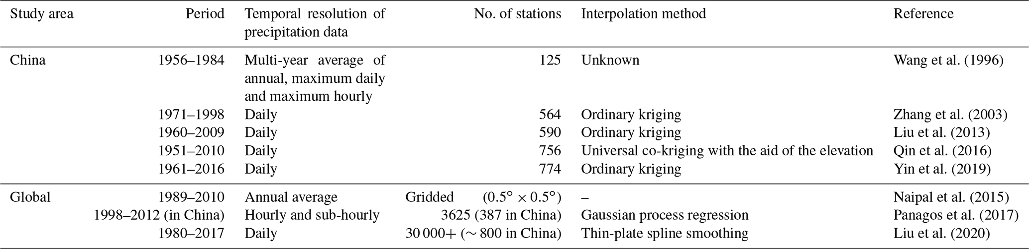
Daily rainfall data from 2381 meteorological stations over mainland China (Fig. 1) over the period of 1951–2014 were measured with simple rain gauges. The data were collected and quality controlled by the National Meteorological Information Center of China Meteorological Administration. Daily data were collected all year around at these stations. An effective year of the daily data was defined as a year when there were no missing data for 1 or more months in the year, and a missing month was defined as a month when there were more than 6 missing days in the month. The missing records in the effective years were input as zero. Based on this definition, the number of effective years ranged from 18 to 54 years. Most of the stations (88 %) have data for more than 50 years.
Hourly rainfall data from the same 2381 stations with daily data (Fig. 1) were collected by siphon rain gauges or tipping bucket rain gauges and also quality controlled by the National Meteorological Information Center of China Meteorological Administration. The period of record for hourly data was from 1951 to 2018. The start year of the data varied because data collection commenced in different years. Observation was suspended in the snowy season, which resulted in some missing months in winter for stations in the northern part of China. There were 932 (39 %) stations with data for the whole year, 550 (23 %) stations from April to October and 421 (18 %) stations from May to September.
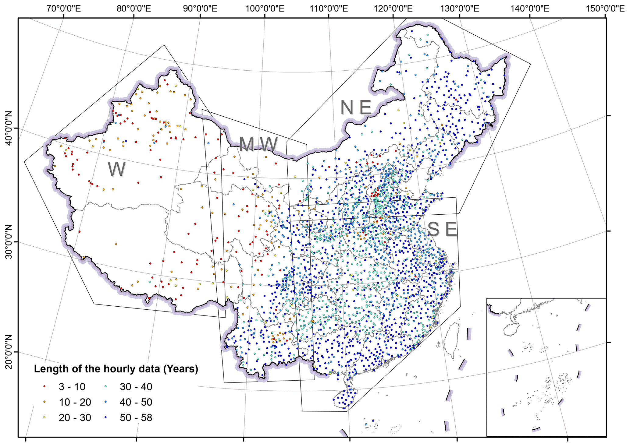
Figure 1Spatial distribution of stations with daily and hourly rainfall data and the length of the hourly data. Western, mid-western, north-eastern and south-eastern regions were abbreviated as W, MW, NE and SE, respectively.
The missing data were handled according to the following criteria: (a) a day with more than 4 missing hours was defined as a missing day; (b) a month with more than 6 missing days was defined as a missing month; (c) a year with any missing month in its wet season was defined as a missing year. The wet season for stations north of 32∘ N was from May to September, and for those south of 32∘ N was from April to October. Missing years were removed, and missing hours in the remaining effective years were input into two categories: (a) the missing period is followed by a non-zero record, which recorded the accumulated rainfall amount in the missing period based on data notes; (b) the missing period is followed by zero. In the first case, each missing hour and the following non-zero hour were assigned the mean value of the non-zero record in these hours. For the second case, the missing hours were input as zero value.
Data at 1 min intervals were collected from 62 stations in mainland China (Fig. 2; and were used in Yue et al., 2020a). Data from station No. 1–18 have effective years of 29–40 and cover the period of 1961(1971)–2000. Data from stations No. 19–62 have effective years of 2–12 and cover the period of 2005–2016. The missing data in the effective years were assumed to be zero.
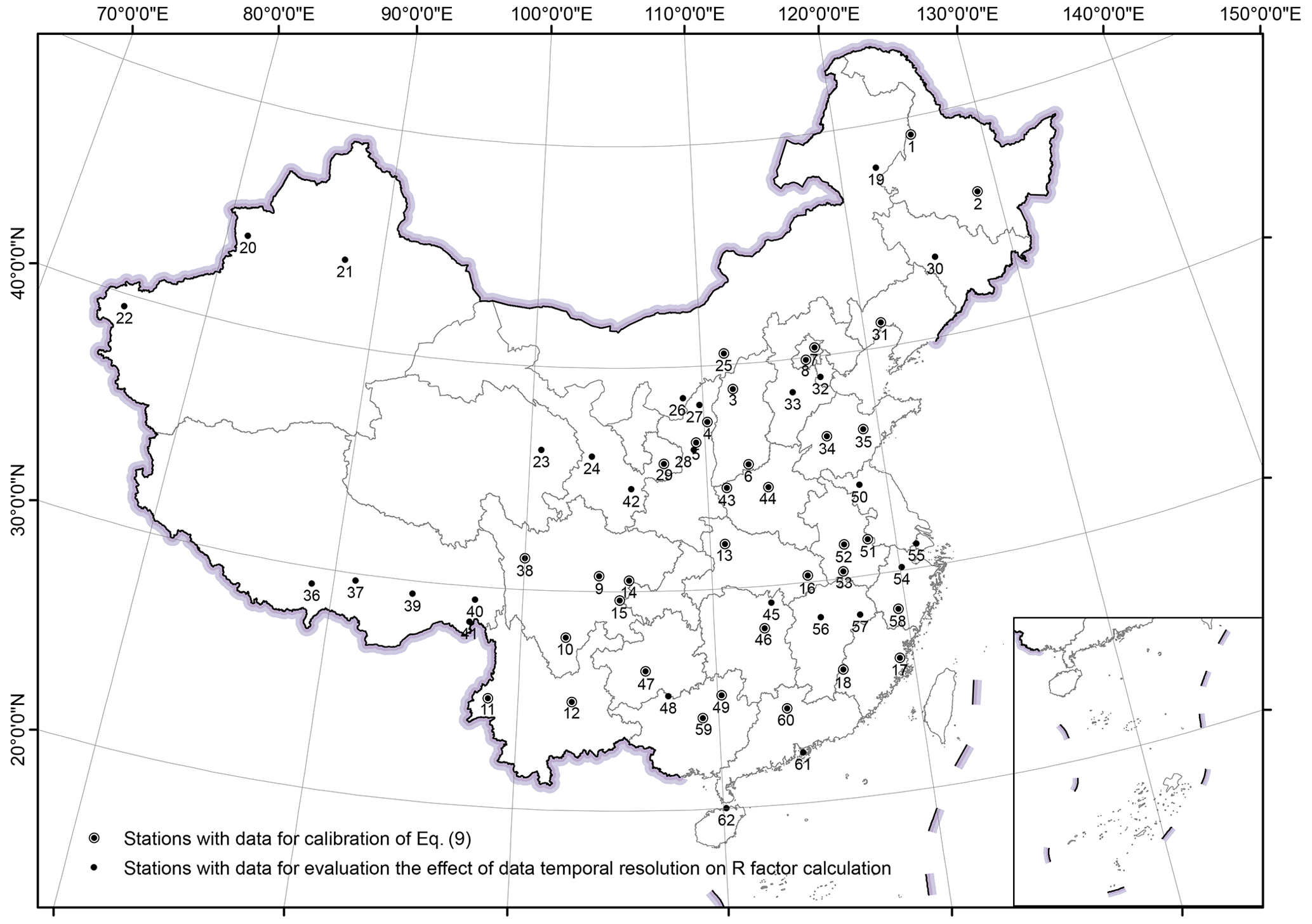
Figure 2Spatial distribution of the stations with 1 min rainfall data.
2.1.2 Published rainfall erosivity maps for China
The existing rainfall erosivity maps were collected and compared with the maps generated in this study. The current national R-factor map and 1-in-10-year EI30 map are based on daily rainfall data only over the period from 1961 to 2016 from 774 stations in China (Yin et al., 2019). Another R-factor map shown in the discussion section of this study (Fig. 12) was based on the global rainfall erosivity dataset published by Joint Research Centre – European Soil Data Centre (ESDAC; Panagos et al., 2017).
2.2 Calculation of rainfall erosivity using 1 min, hourly and daily data
One-minute and hourly data were first separated into storm events. A continuous period of ≧ 6 h of no-precipitation was used to separate storms (Wischmeier and Smith, 1978). Storms with the amount of ≧ 12 mm were defined as erosive events (Xie et al., 2000) and were used to calculate the rainfall erosivity factors.
The R-factor was calculated using Eqs. (1)–(3) (USDA-ARS, 2013):
where EI30 (event rainfall erosivity, MJ mm ha−1 h−1) is the product of the total storm energy E (MJ ha−1) and the maximum 30 min intensity I30 (mm h−1); , where N is the number of effective years, and means there are m erosive storm events in the ith year. For each storm event, rainfall was divided into l time intervals depending on the temporal resolution of rainfall data. The total storm energy E was the sum of the energy for each time interval r, which was the unit energy er (energy per mm of rainfall, MJ ha−1 mm−1) multiplied by the rainfall amount Pr (mm) for each time interval. And ir was the intensity (mm h−1) of the rth interval. I30 (mm h−1) was the maximum intensity over 30 consecutive minutes for each storm event. For hourly data, the I30 was assumed to be the same as the maximum 1 h intensity.
The 1-in-10-year EI30 with 1 min or hourly data was obtained by fitting the generalized extreme value distribution (GEV). The GEV distribution is a family of probability distributions of Gumbel, Fréchet and Weibull, and it can be denoted as G (μ, σ, ξ) with parameters μ (location), σ (scale), and ξ (shape) (Coles, 2001):
where x is the annual maximum storm EI30 (MJ mm ha−1 h−1), , σ>0 and . The extreme quantiles of the annual maximum EI30 (Xp) can be obtained by inverting Eq. (4):
where . The 1-in-10-year EI30 was the value of Xp when p was .
Parameter values for the GEV distribution were estimated using the L-moments method (Hosking, 1990).
Since hourly data aggregation of 1 min data and temporal variation in rainfall intensity is reduced, erosivity factor values computed with hourly data would be underestimated. Therefore, the R-factor and 1-in-10-year EI30 values computed with hourly data need to be adjusted by multiplying conversion factors of 1.871 and 1.489 (SI units), which were fitted by 1 min rainfall data from 62 stations over mainland China (Yue et al., 2020a). Erosivity factors from daily data were also obtained as described in Sect. 2.3. The R-factor using daily data was the mean annual daily erosivity. Daily rainfall erosivity was obtained by the following equation developed by Xie et al. (2016):
where Pdaily is the daily precipitation (≥ 10 mm) and parameter α is 0.3937 in the warm season (May to September) and 0.3101 in the cold season (October to April).
The 1-in-10-year EI30 using daily data was the 1-in-10-year daily erosivity adjusted with a conversion factor of 1.17 based on 1 min data from 18 stations in China (Yin et al., 2019). And the 1-in-10-year daily erosivity was obtained by calibrating the GEV distribution parameters as Eqs. (4)–(5) and the x in the functions was replaced by the annual maximum daily erosivity.
2.3 Rainfall erosivity for individual stations
Hourly data from 2381 stations were used to produce the R-factor and the 1-in-10-year EI30 maps. Due to the annual variability of rainfall erosivity, stations with less than 22 effective years should be excluded (Wischmeier and Smith, 1978). However, 133 out of 150 stations in western China have less than 22 effective years (Fig. 1). Once these stations are removed, the western stations would be too sparse, which would reduce the interpolation accuracy of the rainfall erosivity map. To fill the gap due to the insufficient number of years, daily rainfall data with longer periods of record were used to adjust erosivity values based on hourly data at the same station.
When the effective years of hourly data were not less than those of daily data for 871 out of 2381 station, no adjustment of the R-factor was made. For the remaining 1510 stations, the R-factor from hourly data was then adjusted by a relationship between the mean annual rainfall and the R-factor computed with hourly data as follows (Zhu and Yu, 2015):
where Rh_adj is the adjusted R-factor, Rhour is the estimated R-factor using hourly rainfall data, Pd is the mean annual precipitation of longer period (period of the daily data), and Ph is the mean annual precipitation of shorter period (period of the hourly data).
The exponent value of 1.481 was estimated based on a power relationship between the mean annual precipitation and the R-factor, and the latter was determined using 1 min and daily rainfall data of 35 stations in China (Fig. 2). All the daily and 1 min data shared common periods of record of more than 10 years.
where Rmin is the R-factor (MJ mm ha−1 h−1 a−1), and Pm is the mean annual precipitation (mm) using 1 min data. The coefficient of determination (R2) is 0.776 for Eq. (8).
The 1-in-10-year EI30 for the stations was adjusted in a similar fashion. No adjustment is needed for 89 % of the stations where the effective years of the hourly data were not less than 22 years. For the remaining 11 % of the station, the 1-in-10-year EI30 was estimated with daily data.
The record length was 22 to 29 years for 16 (0.7 %) stations, 30 to 39 years for 44 (1.8 %) stations, 40 to 49 years for 216 (9.1 %) stations, more than 50 years for 2105 (88.4 %) stations when these adjustments were made.
2.4 Spatial interpolation and cross-validation
The erosivity maps were obtained using the method of universal kriging with the annual rainfall as a co-variable. The mean annual rainfall was computed using daily rainfall data and was interpolated using ordinary kriging, and interpolated mean annual rainfall was then used to interpolate the R-factor value using universal kriging. Both the mean annual precipitation and the erosivity factor were interpolated first for each of the four regions separately (Fig. 1; Li et al., 2014) and then combined to obtain annual precipitation and erosivity maps over China. Buffer areas were used to avoid discontinuity along region boundaries (Li et al., 2014).
To evaluate the efficiency of interpolation models, a leave-one-out cross-validation method was applied to each region. Symmetric mean absolute percentage error (sMAPE) and Nash–Sutcliffe coefficient of efficiency (NSE) were used for the assessment:
where n is the number of stations, Fi is the estimated value through universal kriging for the ith station using data from surrounding stations and Ai is the observed value at the ith station.
2.5 Accuracy assessment of erosivity maps
To evaluate the accuracy of the new erosivity maps, erosivity factors using 1 min data were assumed as the “true” values to calculate relative errors since they are most accurate. For the R-factor, 1 min data for 62 stations were used. For 1-in-10-year EI30, 1 min data for 18 stations (No. 1–18; Fig. 2) of the 62 stations with more than 22 years were used. The cross-validation results for these stations from the interpolation of the two erosivity maps were compared to the values from 1 min data to calculate relative errors. Since the relative error tends to be high for stations with small R-factor values, the overall relative error for erosivity maps was represented with the median of the absolute value of the relative error for all the stations.
2.6 Comparative evaluation of the existing and new erosivity maps
Existing erosivity mapping at the national scale in mainland China usually uses daily rainfall data from about 500–800 stations. The R-factor and 1-in-10-year EI30 maps of Yin et al. (2019) were taken as references to evaluate the improvement in the accuracy of the erosivity maps generated in this study. Their relative errors were also obtained with 1 min data as described above.
New erosivity maps in this study followed a procedure that is different from Yin et al. (2019) mainly in three aspects: (1) temporal resolution (hourly vs. daily); (2) number of stations (2381 stations vs. 744 stations); (3) interpolation method (universal kriging vs. ordinary kriging).
To evaluate the effect of the temporal resolution on R-factor and 1-in-10-year EI30, data from the same set of stations were used, and the only difference was that in temporal resolution. Hourly and daily rainfall data with the same period as the 1 min data at the 62 stations were used to calculate R-factors and 1-in-10-year EI30 respectively. Erosivity factors from 1 min data are regarded as the most accurate values. The relative errors of erosivity factors from daily and hourly data were computed for evaluating accuracy.
To evaluate the effect of station density, maps were compared with the only difference in the number of stations. Hourly data from 774 stations (the same set of stations in Yin et al., 2019) and from 2381 stations (used in this study) were used to generate two separate erosivity maps. R-factor and 1-in-10-year EI30 values were compared using a leave-one-out cross-validation method region by region. The sMAPE was calculated for accuracy assessment.
To evaluate the effect of interpolation methods, maps were compared with the only difference in interpolation methods. Ordinary kriging and universal kriging with the mean annual rainfall as the co-variable were applied for the R-factor and 1-in-10-year EI30 computed using hourly data from 2381 stations. Both interpolation methods were applied to each of four different regions as shown in Fig. 1, and leave-one-out cross-validation results were compared. The sMAPE was calculated to evaluate the accuracy of interpolated values.
The framework of this study is shown in Fig. 3.
3.1 Accuracy evaluation on erosivity maps
With erosivity maps from Yin et al. (2019) as references, this study shows improvement in the accuracy of estimated R-factor and 1-in-10-year EI30 (Figs. 4 and 5; Table 2). The spatial distribution of the absolute relative errors of the maps from this study is shown in Fig. 6.
The R-factor values in the map of Yin et al. (2019) were underestimated where the R-factor was relatively high and overestimated where the R-factor was relatively low. The improvement was particularly noticeable for western China (R < 1000 MJ mm ha−1 h−1 a−1) and the south-eastern coastal region (R > 10 000 MJ mm ha−1 h−1 a−1).
Relative errors of erosivity factors at the stations from the two maps are shown in Fig. 5a and b. Those with the relative error of more than 100 % were all in the western (W) or mid-western (MW) region. The absolute relative error for the R-factor in this study and Yin et al. (2019) was no more than 19 % for mid-western (MW), north-eastern (NE) and south-eastern (SE) regions (Table 2). However, there are some extremely high relative error values in Yin's map which were found to be located in the MW region (Fig. 5a). The median values of the absolute relative error in the R-factor in western (W) region were 16.2 % and 161.6 %, respectively, for this study and Yin et al. (2019). For 1-in-10-year EI30, the median values of the absolute relative error were 13.5 % for this study and 20.6 % for Yin et al. (2019), indicating a smaller improvement in the mid-western and eastern regions compared to the improvement for the R-factor map (Table 2, Fig. 5b). The relative errors of the 1-in-10-year EI30 in this study were concentrated in the range of −10 % to +10 %, whereas those in Yin et al. (2019) were concentrated in the range of −25 % to −15 % and +15 % to +25 % (Fig. 5c). The western region was excluded in the evaluation of the 1-in-10-year EI30 map because the record length of the 1 min data was too short to estimate 1-in-10-year event erosivity.
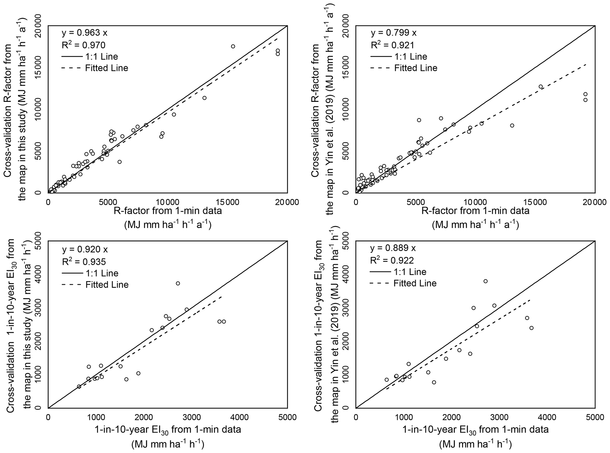
Figure 4Comparison of the R-factors and 1-in-10-year EI30 of the cross-validation values at the station of the maps and the values from 1 min data. The graphs on the left are the evaluation of the maps generated in this study, and those on the right are the evaluation of the maps generated by Yin et al. (2019).
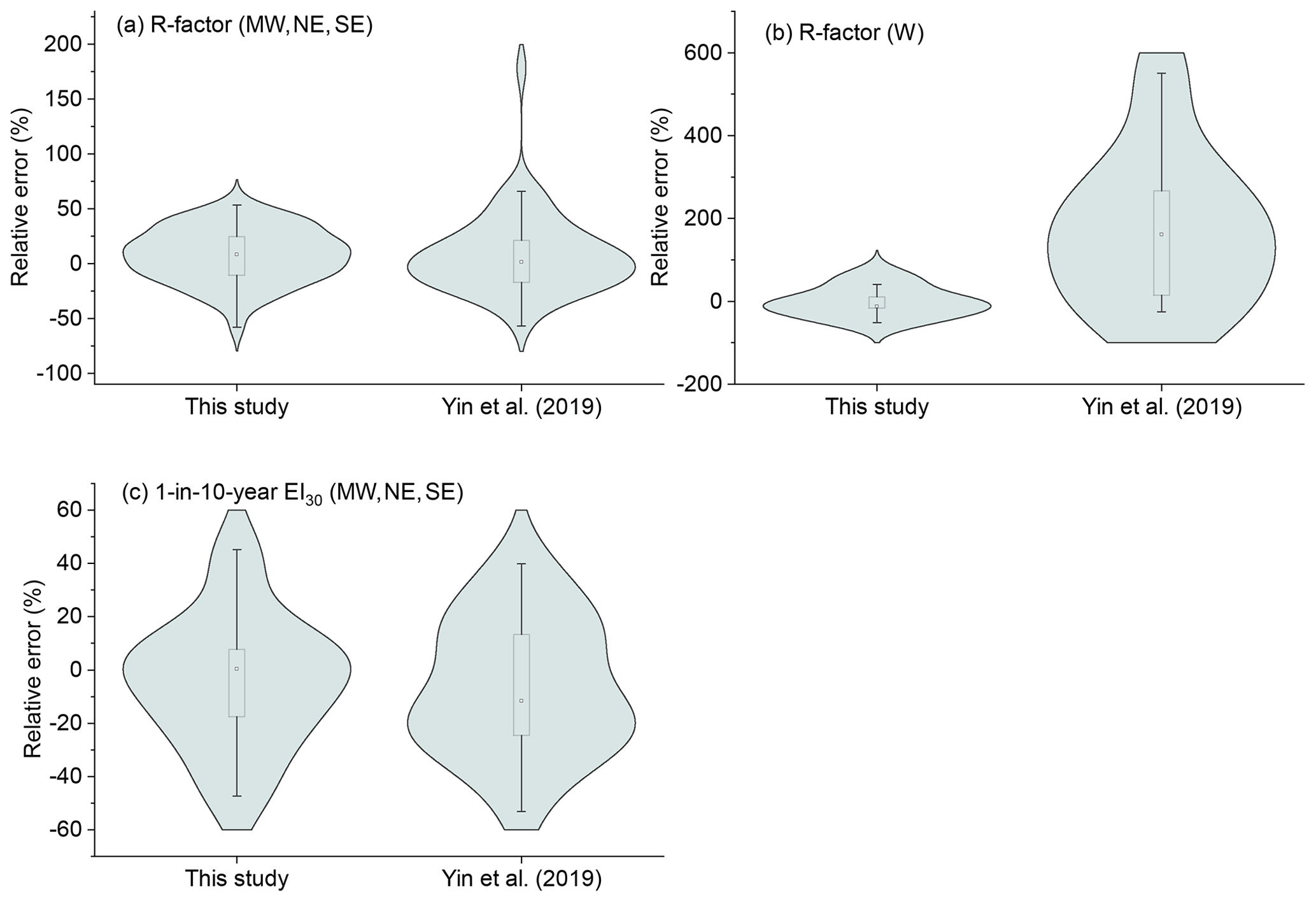
Figure 5The relative errors of the R-factor (a for regions MW, NE, SE; b for region W) and 1-in-10-year EI30 (c for regions ME, NE, SE) maps.
Table 2The statistical characteristics of the absolute relative errors of the erosivity factors from the maps.
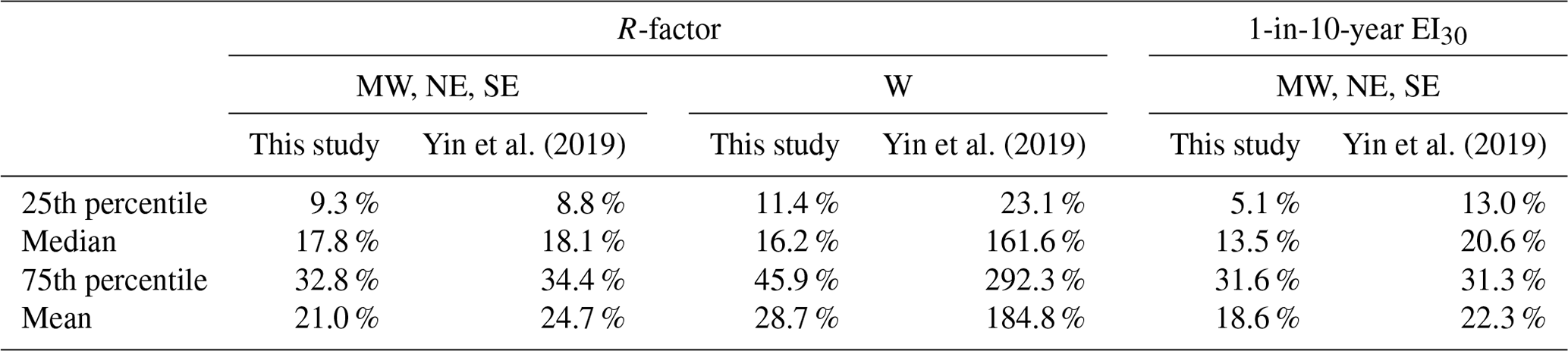
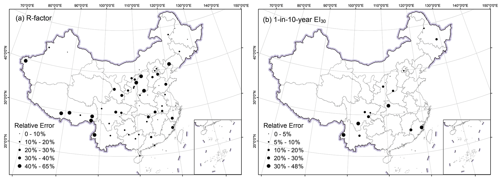
Figure 6Spatial distribution of the absolute relative errors in the map of R-factor for 62 stations (a) and in the map of 1-in-10-year EI30 for 18 stations (b) with 1 min observation data.
3.2 Erosivity maps and improvements over previous studies
The R-factor in China generally decreased from the south-eastern to the north-western region (Fig. 7a), ranging from 0 to 25 300 MJ mm ha−1 h−1 a−1. The map of 1-in-10-year EI30 shows a similar spatial pattern as that of the R-factor (Fig. 7b), ranging from 0 to 11 246 MJ mm ha−1 h−1. Zero R-factor value is found at Turpan, Xinjiang Uygur Autonomous Region, where the mean annual rainfall is only 7.8 mm. The maximum of the R-factor (more than 20 000 MJ mm ha−1 h−1 a−1) is found in the southern part of the Guangxi and Guangdong provinces, along the South China Sea, where the mean annual rainfall is more than 2500 mm.
In addition to the overall trend, some local-scale characteristics could be identified. For the R-factor map, in the western region, the wetter region in north-western China was located in the west of Dzungaria Basin and along Tian Shan, which has been captured on the map. Some statistical characteristics of the new maps of the erosivity factors are shown in Table 3 based for soil erosion and hydrological zones in China (Fig. 8).
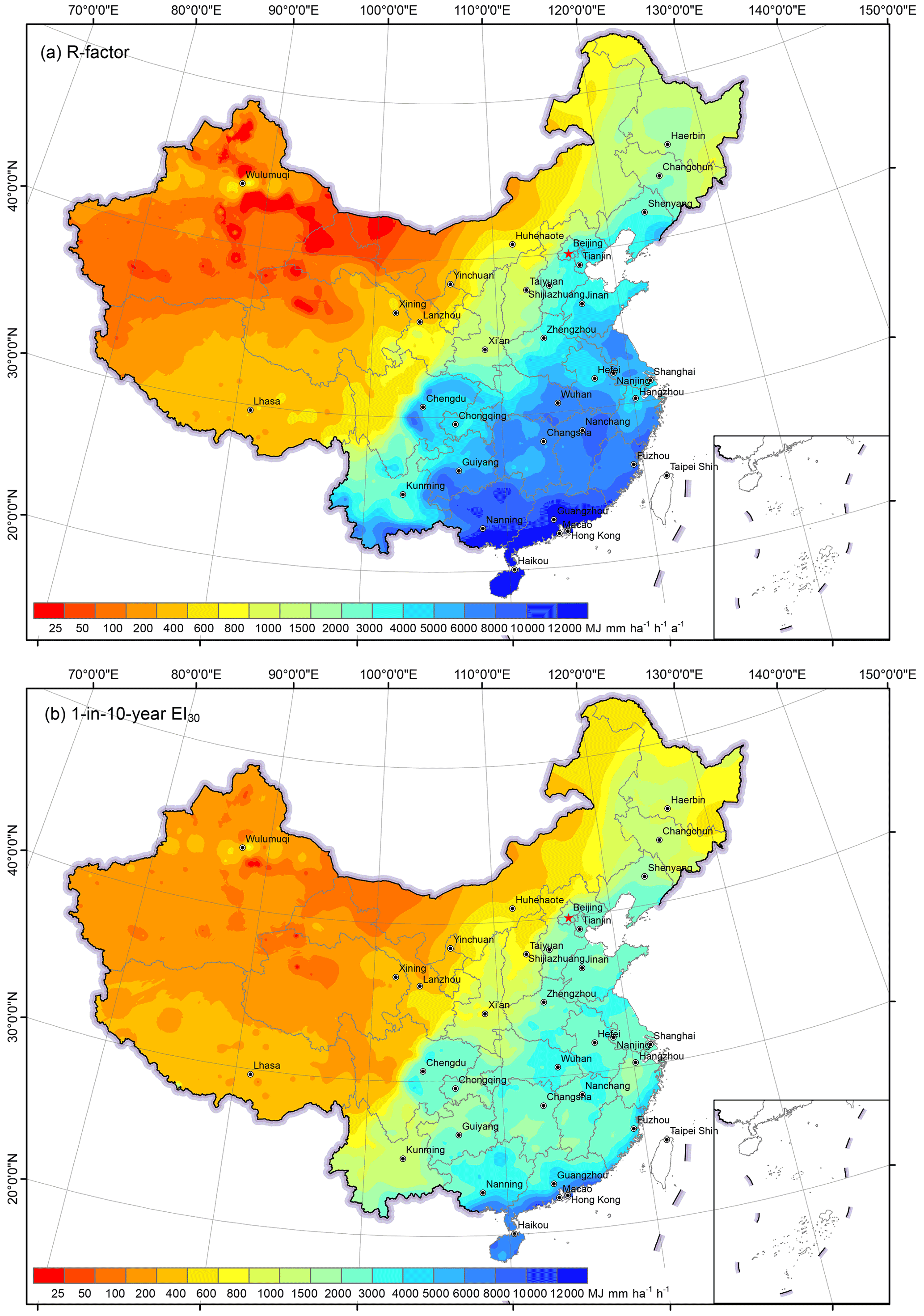
Figure 7R-factor (a) and 1-in-10-year EI30 (b) over the study area based on hourly data from 2381 stations.

Figure 8Zoning schemes.
Table 3Statistical characteristics of R-factor and 1-in-10-year EI30 in soil erosion and hydrological zonings.
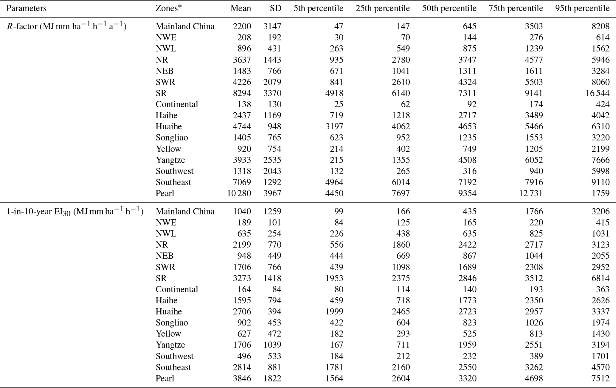
* The zonings are shown in Fig. 8.
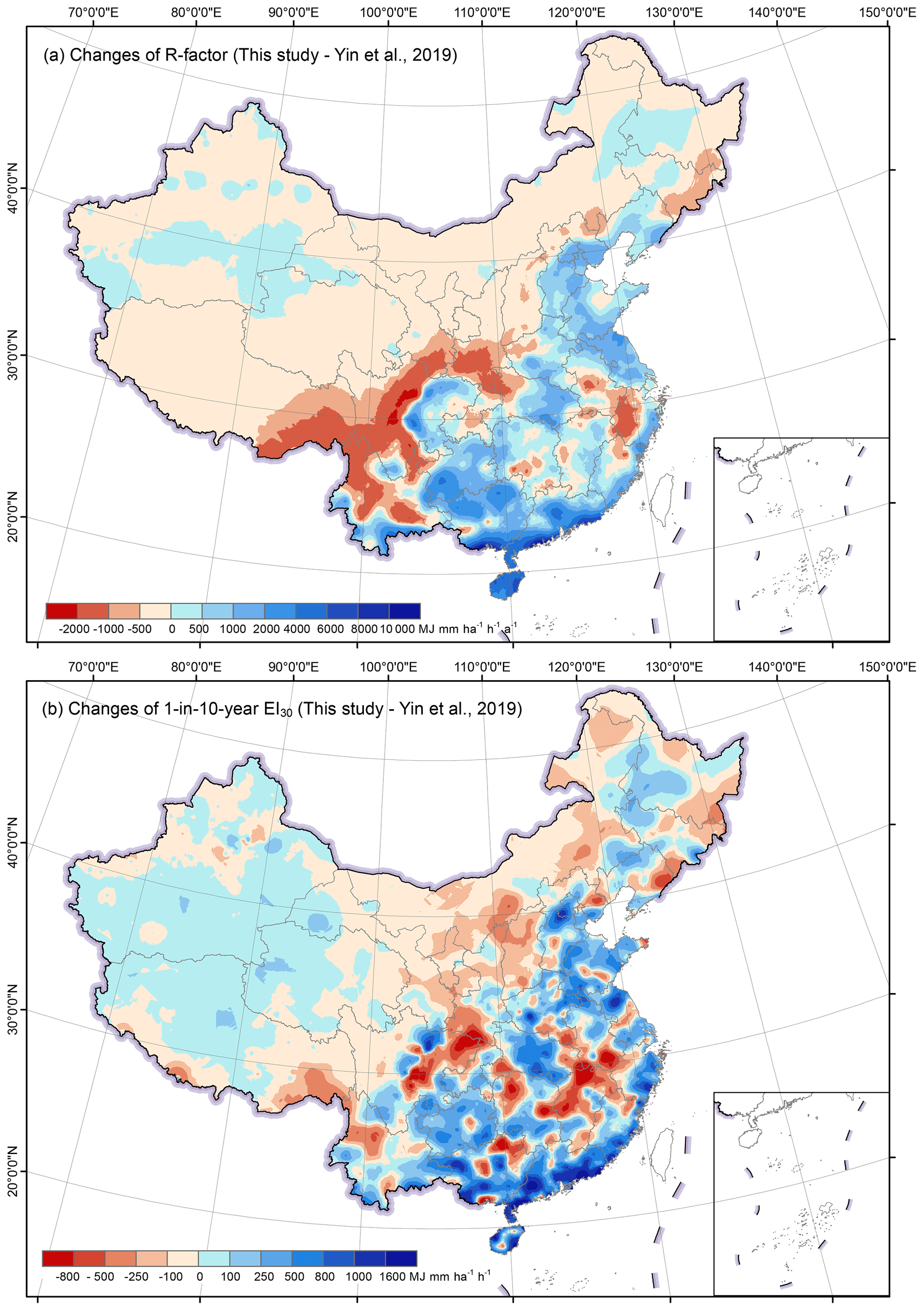
Figure 9Differences of the R-factor (a) and the 1-in-10-year EI30 (b) comparing with the previous study.
Comparing with the maps in Yin et al. (2019), the new maps can be quite different at some local areas (Fig. 9a and b). The R-factor in the new map was higher for most of the south-eastern region and lower for most of the middle and western regions, especially for the south-western area (Fig. 9a). However, the 1-in-10-year EI30 map shows a similar pattern as that of R-factor, and the overestimation in Yin et al. (2019) seems to be more pronounced for some hilly regions in southeastern China (Fig. 9b).
3.3 Evaluation on the improvement of the erosivity maps
3.3.1 Effect of data temporal resolution
Figure 10 shows that the R-factor estimated from daily data (Eq. 6) is underestimated when the R value is higher than 10 000 MJ mm ha−1 h−1 a−1 and slightly overestimated when the value is lower than 2000 MJ mm ha−1 h−1 a−1. The model using hourly data improved the accuracy by about 11.1 % (median value of the relative error) compared to that from daily data (Fig. 10). Estimated 1-in-10-year EI30 would be underestimated using hourly and daily data, and the underestimation is greater if daily data were used (Fig. 10). Unlike the R-factor, the 1-in-10-year EI30 was not noticeably improved with an increase in the temporal resolution from daily to hourly data, probably due to the fact that the 1-in-10-year EI30 values estimated using daily data in Yin et al. (2019) had already been multiplied by a conversion factor of 1.17 to correct the 1-in-10-year daily erosivity to approximate the 1-in-10-year event EI30 from 1 min data.
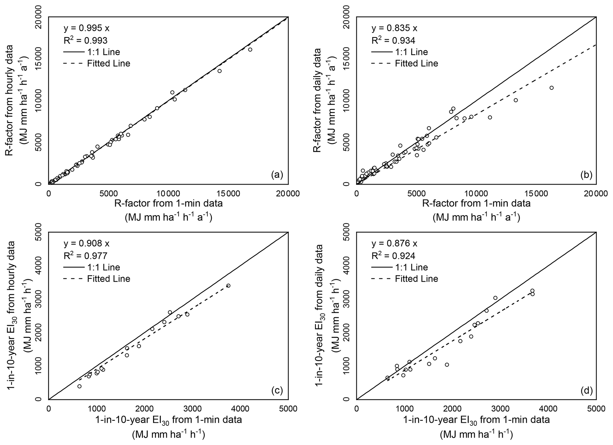
Figure 10Comparison of the R-factor (a, b) and 1-in-10-year EI30 (c, d) estimated from hourly (a, c) and daily (b, d) rainfall data at the stations.
3.3.2 Effect of the station density
Interpolation for the western (W) region had the lowest NSE value compared to other regions, which may be caused by the low station density (Fig. 1) and the lower spatial correlation of rainfall. The fitted semivariogram for the R-factor in the western region had a range of 35 km, whereas the ranges for mid-western (MW), north-eastern (NE) and south-eastern (SE) regions were 288, 261 and 1235 km, respectively.
A comparison of cross-validation between the two maps with different station densities shows that the interpolation with denser stations can improve the accuracy by 2.6 %–15.4 % for the R-factor based on the sMAPE index and by 1.4 %–31.8 % for 1-in-10-year EI30 (Table 4) when the station density increased. The NSE can increase by 0.013 to 0.110 for the R-factor. For the 1-in-10-year EI30, the NSE decreased by 0.001 to 0.096 for western (W), mid-western (MW) and south-eastern (SE) regions and increased by 0.038 for the north-eastern (NE) region.
For the R-factor, in the western (W) region, the station density doubled (increased from 36 600 to 21 200 km2 per station), and the accuracy improved by 15.4 %, whereas the sMAPE of 53.3 % was still high with this increase in station density. In the mid-western (MW) region, the station density tripled (from 13 900 to 4800 km2 1 station) and the accuracy was improved by 11.1 % based on the sMAPE index from 30.7 % to 19.6 %. In north-eastern (NE) and south-eastern (SE) regions, the station density tripled and quadrupled, respectively, and the accuracy increased about 2.5 %. For 1-in-10-year EI30, the improvement was 31.8 % in the western (W) region and 19.6 % in the mid-western (MW) region. The improvement was mainly in western regions, and the station density in the eastern China before the increase is enough to describe the spatial variation of the R-factor and the 1-in-10-year EI30. It can be inferred that when there were less than about 10 000 km2 per station, the increase of the site density has little impact on the improvement of the interpolation (Fig. 11).
Table 4Comparison of cross-validation results for erosivity maps interpolated based on data from 774 and 2381 stations.
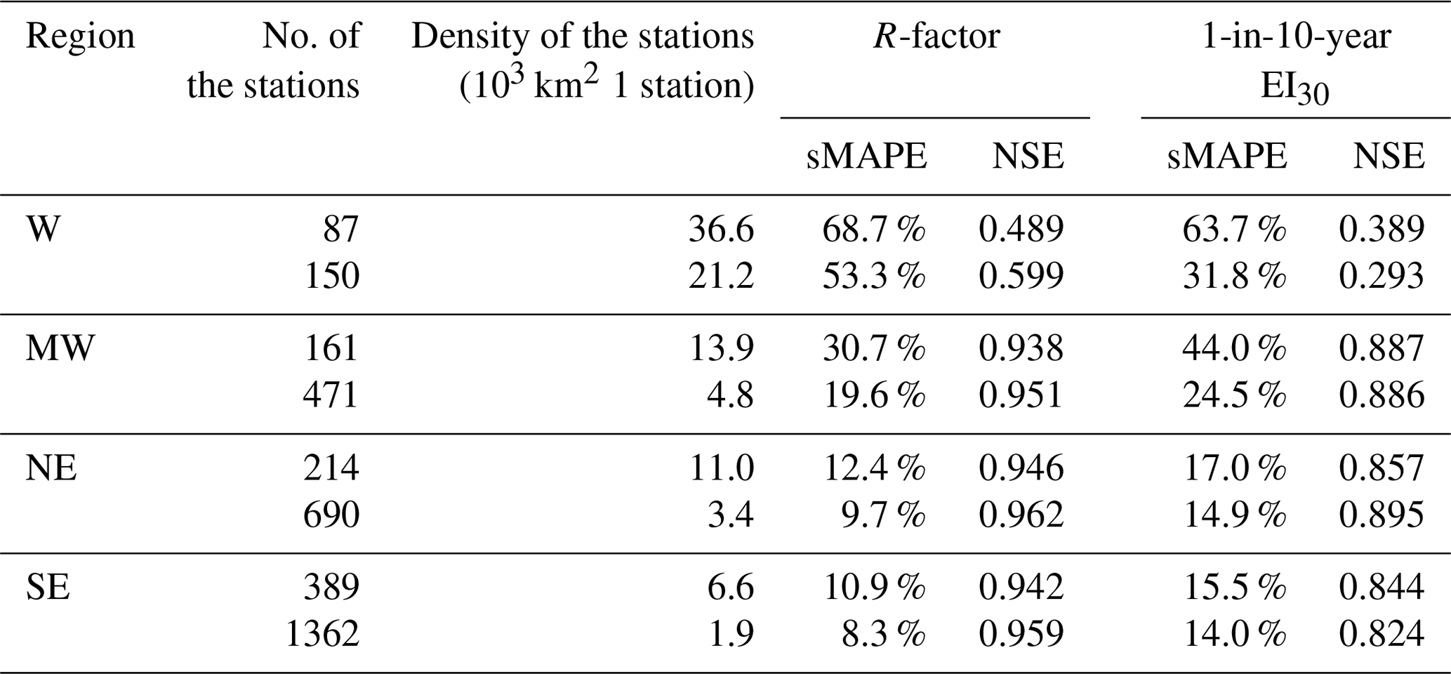

Figure 11Improvement of the interpolation with the increase of station density. Data were from the 774 and 2381 stations in the 4 different regions.
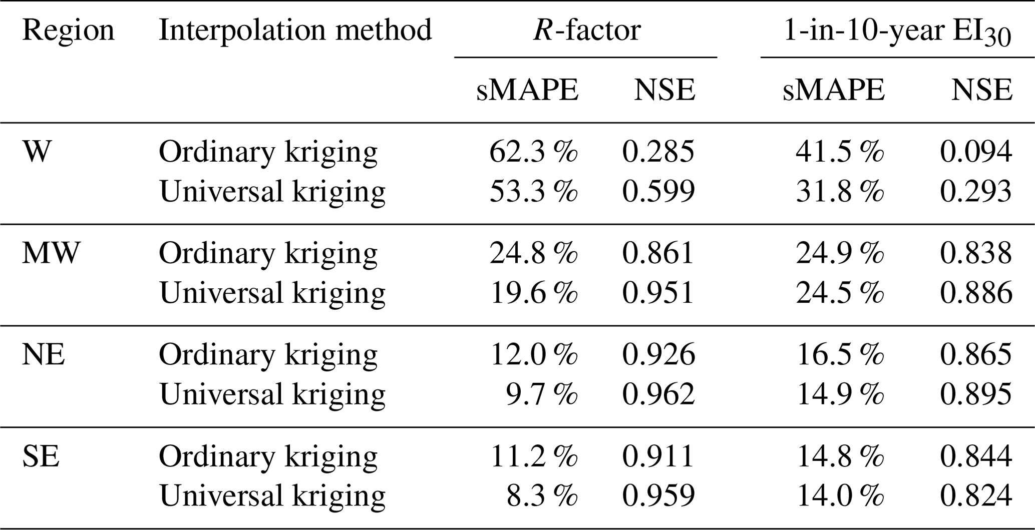
3.3.3 Effect of the interpolation method
For the R-factor, cross-validation of ordinary kriging and universal kriging with the mean annual rainfall as the co-variable (Table 5) shows that universal kriging improved the interpolation accuracy by 2.3 %–9.0 % (sMAPE) compared to ordinary kriging. In the western (W) region, the NSE increased from 0.285 (ordinary kriging) to 0.599 (universal kriging). Therefore, it is better to use universal kriging instead of ordinary kriging when generating the R-factor map, especially in western China where the station density is low. For the 1-in-10-year EI30, universal kriging improved the accuracy by 0.4 %–9.7 % (sMAPE). In the western (W) region, the accuracy improved by 9.7 % and the NSE increased from 0.094 (ordinary kriging) to 0.293 (universal kriging).
Table 5Cross-validation of the interpolated R-factor and 1-in-10-year event EI30 using ordinary kriging and universal kriging.
This study has produced quality R-factor and 1-in-10-year EI30 maps with hourly data from 2381 stations over mainland China, which are shown to be a noticeable improvement over the maps that are currently available for China (Yin et al., 2019; Table 1). The improvement of the R-factor map over previously published R-factor maps can be attributed to the increase in the temporal resolution from daily to hourly data, whereas that of 1-in-10-year EI30 map to the increase of the station density in comparison with those of Yin et al. (2019). There are mainly two reasons for this. First, 1-in-10-year event EI30 values estimated from the daily data had already been adjusted to those from the 1 min data by multiplying a conversion factor of 1.17 (Yin et al., 2019), which resulted in no obvious improvement from the daily data to the hourly data. Second, the 1-in-10-year event EI30 associated with extreme rainfall event intrinsically has a high spatial variability in comparison to the R-factor as shown in Table 4. The accuracy of spatially interpolated rainfall erosivity was more sensitive to the station density when the station density is low. Hence the improvement of the map of the 1-in-10-year EI30 was mainly a result of the increase of the station density, especially for the western (W) and the mid-western (MW) regions with a low station density.
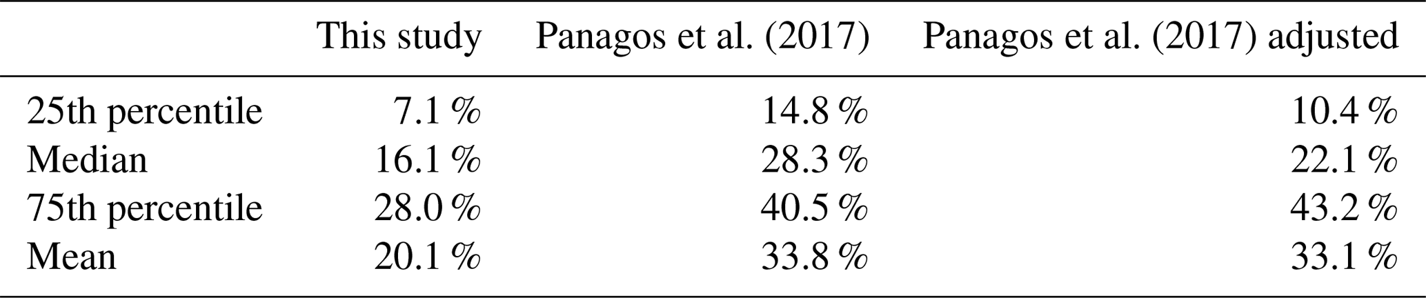
Comparison with a world map of rainfall erosivity was also undertaken for mainland China. Panagos et al. (2017) produced the Global Rainfall Erosivity Database with hourly and sub-hourly rainfall data from 3625 stations from 63 countries. This database could be used for comparison of rainfall erosivity among different regions in the world. In their study, hourly data from 387 stations in China were used. Figure 12 shows that the R-factor for China extracted from Panagos et al. (2017) is systematically underestimated by about 30 % for most areas in China, whereas it is overestimated in the Tibetan Plateau (cf. Fig. 7a). The reason for the underestimation may be that the R-factor calculated from hourly data applied a conversion factor (CF30) that was developed from the R-factor values computed with 60 min data to those with 30 min data in Panagos et al. (2015b), rather than using an adjustment factor based on breakpoint data (CFbp) or 1 min data (CF1). Breakpoint data were used for the USLE (Wischmeier and Smith, 1965, 1978), RUSLE (Renard et al., 1997) and 1 min data for this study. Previous research has shown the difference between CF30 and CFbp (CF1) can result in an underestimation of R-factor by about 20 % (Auerswald et al., 2015; Yue et al., 2020a). Table 6 shows that the relative error of the map from Panagos et al. (2017) could reduce by about 6.2 % after multiplying by a conversion factor of 1.253, which was calibrated by Yue et al. (2020a) for converting the R-factor from 30 min data to 1 min data. Because the cross-validation values from the map of Panagos et al. (2017) were not available, values extracted from the maps were used instead to compare with the values from 1 min data at the 62 stations. Erosivity values based on the adjusted maps are still generally underestimated. The reason could be that the equation for estimating the storm energy (E) from rainfall intensity used in Panagos et al. (2017) was from the RUSLE (Renard et al., 1997), and the equation is known to cause underestimation of the storm energy up to 10 % in previous studies (McGregor et al., 1995; Yin et al., 2017). Because of this, the equation for estimating the storm energy (E) in RUSLE (Renard et al., 1997) was then modified in RUSLE2 (USDA-ARS, 2013), which was adopted in this study.
The R-factor in the Tibetan Plateau varies from 0 to 12 326 MJ mm ha−1 h−1 a−1 in Panagos et al. (2017) and from 5 to 4442 MJ mm ha−1 h−1 a−1 in this study. The former was derived from a Gaussian process regression (GPR) model and a number of monthly climate variables from the WorldClim database, such as the mean monthly precipitation, mean minimum, and average and maximum monthly temperature. The GPR model was calibrated using the site-specific R-factor values and these climate variables, which may not applicable for sites at high altitude, as none of the observation sites was located in the Tibetan Plateau region. The GPR model might be the main reason for the overestimation of the R-factor in the Tibetan Plateau where the R-factor was expected to be underestimated just like any other regions.

Figure 12R-factor map of the study area extracted from Panagos et al. (2017) and the evaluation of the map based on 62 stations with 1 min data.
Table 6Comparison of the statistical characteristics of the relative errors of the R-factor extracted from the map generated in this study and extracted from Panagos et al. (2017) (original and adjusted). The adjusted map of Panagos et al. (2017) was the original map multiplying by a conversion factor of 1.253, which was calibrated by Yue et al. (2020a) for converting the R-factor from 30 min data to 1 min data.
Although this study provides improved erosivity maps in comparison with previous studies, errors remain inevitably. The uncertainty of the estimated R-factor and 1-in-10-year erosivity values from this study mainly comes from the following sources: first, the KE–I model for estimating kinetic energy (KE) from the precipitation intensity (I). The KE–I model used in this study is from RUSLE2 (USDA-ARS, 2013), and raindrop disdrometer observation data need to be collected to calibrate the KE–I relationship. Second, estimation of the erosivity factors was based on hourly data, and conversion factors were developed based on 1 min rainfall data from 62 stations (Fig. 2). Hourly data bring information loss in the estimation of instant precipitation intensity comparing with breakpoint data. Third, there is an adjustment of the R-factor for the stations with a small number of effective years (Eq. 7). This was based on a power function relationship (Eq. 8) between the mean annual precipitation and rainfall erosivity using 1 min and daily rainfall data of 35 stations. The magnitude of uncertainty mainly depends on the variation of annual rainfall erosivity. The fourth source is station distribution and density. In western China, the stations were sparsely and unevenly distributed, which affect the interpolation accuracy. The final sources are spatial interpolation technique (universal kriging in this study) and the interpolation procedures, i.e. the division of regions before the interpolation and the mergence of regions after the interpolation. These five sources of uncertainty need to be addressed for any further improvement in erosivity estimation in China.
The rainfall erosivity maps (R-factor and 1-in-10-year EI30) are available at: https://doi.org/10.12275/bnu.clicia.rainfallerosivity.CN.001 (Yue et al., 2020b).
This study has generated new R-factor and 1-in-10-year EI30 maps using hourly and daily rainfall data for the period from 1951 to 2018 from 2381 stations over mainland China. The improvement in the accuracy of these erosivity maps over what are currently available was evaluated in terms of the median absolute relative error and was explained in terms of temporal resolution of data used, station density, and interpolation methods. The following conclusions can be drawn from this study:
-
Comparing with the existing maps for the 62 reference sites, the median absolute relative error in the R-factor map generated in this study was reduced from 18.1 % to 17.8 % for the mid-western and eastern regions, from 161.6 % to 16.2 % for the western region, and for the 1-in-10-year EI30, and from 20.6 % to 13.5 % in the mid-western and eastern regions.
-
The R-factor value varied from 0 to 25 300 MJ mm ha−1 h−1 a−1, and the 1-in-10-year EI30 value was from 0 to 11 246 MJ mm ha−1 h−1. In comparison with the existing maps, new maps of the R-factor and 1-in-10-year event EI30 show a clear decreasing trend from south-eastern to north-eastern China.
-
Improvement in the R-factor map can be mainly attributed to an increase in the temporal resolution from daily to hourly, whereas that in the 1-in-10-year EI30 map to an increase of the station density. The increased station density has led to an improved R-factor and 1-in-10-year EI30 maps for the western regions primarily. The benefit from an increased station density is limited once the station density reached about 1 station per 10 000 km2. As for the interpolation method, universal kriging with the mean annual rainfall as the co-variable performed better than ordinary kriging for all regions, especially for the western regions with sparse weather stations.
TY did the formal analysis, visualization, and original draft writing. SY did the methodology, formal analysis, review, and editing. YX, BY, and BL did the review and editing.
The contact author has declared that neither they nor their co-authors have any competing interests.
Publisher's note: Copernicus Publications remains neutral with regard to jurisdictional claims in published maps and institutional affiliations.
We would like to thank the high-performance computing support from the Center for Geodata and Analysis, Faculty of Geographical Science, Beijing Normal University (https://gda.bnu.edu.cn/, last access: 4 February 2022).
This research has been supported by the National Natural Science Foundation of China (grant no. 41877068) and the National Key Research and Development Program of China (grant no. 2018YFC0507006).
This paper was edited by Min Feng and reviewed by Seyed Hamidreza Sadeghi and four anonymous referees.
Alewell, C., Borelli, P., Meusburger, K., and Panagos, P.: Using the USLE: Chances, challenges and limitations of soil erosion modelling, International Soil and Water Conservation Research, 7, 203–225, https://doi.org/10.1016/j.iswcr.2019.05.004, 2019.
Angulomartínez, M. and Beguería, S.: Estimating rainfall erosivity from daily precipitation records: A comparison among methods using data from the Ebro Basin (NE Spain), J. Hydrol., 379, 111–121, https://doi.org/10.1016/j.jhydrol.2009.09.051, 2009.
Arnoldus, H.: Methodology used to determine the maximum potential average annual soil loss due to sheet and rill erosion in Morocco, FAO Soils Bulletins (FAO), 34, 39–51, 1977.
Auerswald, K., Fiener, P., Gomez, J. A., Govers, G., Quinton, J. N., and Strauss, P.: Comment on “Rainfall erosivity in Europe” by Panagos et al. (Sci. Total Environ., 511, 801–814, 2015), Sci. Total Environ., 532, 849–852, https://doi.org/10.1016/j.scitotenv.2015.05.019, 2015.
Bagarello, V. and D'Asaro, F.: Estimating single storm erosion index, T. ASAE, 37, 785–791, https://doi.org/10.13031/2013.28141, 1994.
Bonilla, C. A. and Vidal, K. L.: Rainfall erosivity in central Chile, J. Hydrol., 410, 126–133, https://doi.org/10.1016/j.jhydrol.2011.09.022, 2011.
Borrelli, P., Diodato, N., and Panagos, P.: Rainfall erosivity in Italy: a national scale spatio-temporal assessment, Int. J. Digi. Earth, 9, 835–850, https://doi.org/10.1080/17538947.2016.1148203, 2016.
Capolongo, D., Diodato, N., Mannaerts, C., Piccarreta, M., and Strobl, R.: Analyzing temporal changes in climate erosivity using a simplified rainfall erosivity model in Basilicata (southern Italy), J. Hydrol., 356, 119–130, https://doi.org/10.1016/j.jhydrol.2008.04.002, 2008.
Coles, S. G.: An introduction to statistical modeling of extreme values, Springer, Series in Statistics, https://doi.org/10.1007/978-1-4471-3675-0, 2001.
FAO: Outcome document of the Global Symposium on Soil Erosion, Food and Agriculture Organization of the United Nations, Rome, 24 pp., 2019.
Ferrari, R., Pasqui, M., Bottai, L., Esposito, S., and Di Giuseppe, E.: Assessment of soil erosion estimate based on a high temporal resolution rainfall dataset, Proc. 7th European Conference on Applications of Meteorology (ECAM), Utrecht, the Netherlands, 12–16, 2005.
Ferro, V., Giordano, G., and Iovino, M.: Isoerosivity and erosion risk map for Sicily, Hydrolog. Sci. J., 36, 549–564, https://doi.org/10.1080/02626669109492543, 1991.
Haith, D. A. and Merrill, D. E.: Evaluation of a daily rainfall erosivity model, T. ASAE, 30, 90–93, https://doi.org/10.13031/2013.30407, 1987.
Hosking, J. R. M.: L-Moments: Analysis and Estimation of Distributions Using Linear Combinations of Order Statistics, J. Roy. Stat. Soc., 52, 105–124, https://doi.org/10.2307/2345653, 1990.
Klik, A., Haas, K., Dvorackova, A., and Fuller, I. C.: Spatial and temporal distribution of rainfall erosivity in New Zealand, Soil Res., 53, 887–901, https://doi.org/10.1071/SR14363, 2015.
Lee, J. H. and Heo, J. H.: Evaluation of Estimation Methods for Rainfall Erosivity Based on Annual Precipitation in Korea, J. Hydrol., 409, 30–48, https://doi.org/10.1016/j.jhydrol.2011.07.031, 2011.
Li, T., Zheng, X., Dai, Y., Yang, C., Chen, Z., Zhang, S., Wu, G., Wang, Z., Huang, C., and Shen, Y.: Mapping near-surface air temperature, pressure, relative humidity and wind speed over Mainland China with high spatiotemporal resolution, Adv. Atmos. Sci., 31, 1127–1135, https://doi.org/10.1007/s00376-014-3190-8, 2014.
Liu, B., Tao, H., and Song, C.: Temporal and spatial variations of rainfall erosivity in China during 1960 to 2009, Geograph. Res., 32, 245–256, 2013.
Liu, Y., Zhao, W., Liu, Y., and Pereira, P.: Global rainfall erosivity changes between 1980 and 2017 based on an erosivity model using daily precipitation data, Catena, 194, 104768, https://doi.org/10.1016/j.catena.2020.104768, 2020.
Lu, H. and Yu, B.: Spatial and seasonal distribution of rainfall erosivity in Australia, Soil Res., 40, 887–901, https://doi.org/10.1071/SR01117, 2002.
McGregor, K., Bingner, R., Bowie, A., and Foster, G.: Erosivity index values for northern Mississippi, T. ASAE, 38, 1039–1047, https://doi.org/10.13031/2013.27921, 1995.
Naipal, V., Reick, C., Pongratz, J., and Van Oost, K.: Improving the global applicability of the RUSLE model – adjustment of the topographical and rainfall erosivity factors, Geosci. Model Dev., 8, 2893–2913, https://doi.org/10.5194/gmd-8-2893-2015, 2015.
Oliveira, P. T. S., Rodrigues, D. B. B., Sobrinho, T. A., Carvalho, D. F. D., and Panachuki, E.: Spatial variability of the rainfall erosive potential in the State of Mato Grosso do Sul, Brazil, Engenharia Agrícola, 32, 69–79, https://doi.org/10.1590/S0100-69162012000100008, 2012.
Panagos, P., Ballabio, C., Borrelli, P., and Meusburger, K.: Spatio-temporal analysis of rainfall erosivity and erosivity density in Greece, Catena, 137, 161–172, https://doi.org/10.1016/j.catena.2015.09.015, 2015a.
Panagos, P., Ballabio, C., Borrelli, P., Meusburger, K., Klik, A., Rousseva, S., Tadić, M. P., Michaelides, S., and Hrabalíková, M.: Rainfall erosivity in Europe, Sci. Total Environ., 511, 801–814, https://doi.org/10.1016/j.scitotenv.2015.01.008, 2015b.
Panagos, P., Borrelli, P., Meusburger, K., Yu, B., Klik, A., Lim, K. J., Yang, J. E., Ni, J., Miao, C., and Chattopadhyay, N.: Global rainfall erosivity assessment based on high-temporal resolution rainfall records, Sci. Rep., 7, 4175, https://doi.org/10.1038/s41598-017-04282-8, 2017.
Pennock, D.: Soil erosion: the greatest challenge to sustainable soil management, Food and Agriculture Organization of the United Nations, Rome, 100 pp., 2019.
Qin, W., Guo, Q., Zuo, C., Shan, Z., Ma, L., and Sun, G.: Spatial distribution and temporal trends of rainfall erosivity in mainland China for 1951–2010, Catena, 147, 177–186, https://doi.org/10.1016/j.catena.2016.07.006, 2016.
Renard, K. G. and Freimund, J. R.: Using monthly precipitation data to estimate the R-factor in the revised USLE, J. Hydrol., 157, 287–306, https://doi.org/10.1016/0022-1694(94)90110-4, 1994.
Renard, K. G., Foster, G. R., Weesies, G. A., Mccool, D. K., and Yoder, D. C.: Predicting soil erosion by water: a guide to conservation planning with the Revised Universal Soil Loss Equation (RUSLE), Agricultural Handbook, USDA-Agricultural Research Service, Washington, D.C., 1997.
Richardson, C., Foster, G., and Wright, D.: Estimation of erosion index from daily rainfall amount, T. ASAE, 26, 153–156, https://doi.org/10.13031/2013.33893, 1983.
Riquetti, N. B., Mello, C. R., Beskow, S., and Viola, M. R.: Rainfall erosivity in South America: Current patterns and future perspectives, Sci. Total Environ., 724, 138315, https://doi.org/10.1016/j.scitotenv.2020.138315, 2020.
Sadeghi, S. H., Zabihi, M., Vafakhah, M., and Hazbavi, Z.: Spatiotemporal mapping of rainfall erosivity index for different return periods in Iran, Nat. Hazards, 87, 35–56, https://doi.org/10.1007/s11069-017-2752-3, 2017.
Selker, J. S., Haith, D. A., and Reynolds, J. E.: Calibration and testing of a daily rainfall erosivity model, T. ASAE, 33, 1612, https://doi.org/10.13031/2013.31516, 1990.
Sheridan, J., Davis, F., Hester, M., and Knisel, W.: Seasonal distribution of rainfall erosivity in peninsular Florida, T. ASAE, 32, 1555–1560, https://doi.org/10.13031/2013.31189, 1989.
Silva, R. M., Santos, C., Silva, J., Silva, A. M., and Neto, R.: Spatial distribution and estimation of rainfall trends and erosivity in the Epitácio Pessoa reservoir catchment, Paraíba, Brazil, Nat. Hazards, 102, 829–849, https://doi.org/10.1007/s11069-020-03926-9, 2020.
USDA-ARS: Science documentation: Revised Universal Soil Loss Equation Version 2 (RUSLE2), USDA-Agricultural Research Service, Washington, D.C., 2013.
Wang, W., Jiao, J., Hao, X., Zhang, X., and Lu, X.: Distribution of rainfall erosivity R value in China, Journal of Soil Erosion and Soil Conservation, 2, 29–39, 1996.
Wischmeier, W. H.: A Rainfall Erosion Index for a Universal Soil-Loss Equation 1, Soil Sci. Soc. Am. J., 23, 246–249, https://doi.org/10.2136/sssaj1959.03615995002300030027x, 1959.
Wischmeier, W. H. and Smith, D. D.: Rainfall energy and its relationship to soil loss, T. Am. Geophys. Un., 39, 285–291, https://doi.org/10.1029/tr039i002p00285, 1958.
Wischmeier, W. H. and Smith, D. D.: Predicting rainfall-erosion losses from cropland east of the Rocky Mountains: Guide for selection of practices for soil and water conservation, Agricultural Handbook, USDA-Agricultural Research Service, Washington, D.C., 1965.
Wischmeier, W. H. and Smith, D. D.: Predicting rainfall erosion losses – a guide to conservation planning, Agricultural Handbook, USDA-Agricultural Research Service, Washington, D.C., 1978.
Xie, Y., Liu, B. Y., and Zhang, W. B.: Study on standard of erosive rainfall, J. Soil Water Conserv., 14, 6–11, https://doi.org/10.13870/j.cnki.stbcxb.2000.04.002, 2000.
Xie, Y., Yin, S. Q., Liu, B. Y., Nearing, M. A., and Zhao, Y.: Models for estimating daily rainfall erosivity in China, J. Hydrol., 535, 547–558, https://doi.org/10.1016/j.jhydrol.2016.02.020, 2016.
Yin, S., Nearing, M. A., Borrelli, P., and Xue, X.: Rainfall Erosivity: An Overview of Methodologies and Applications, Vadose Zone J., 16, 1–16, https://doi.org/10.2136/vzj2017.06.0131, 2017.
Yin, S., Xie, Y., Liu, B., and Nearing, M. A.: Rainfall erosivity estimation based on rainfall data collected over a range of temporal resolutions, Hydrol. Earth Syst. Sci., 19, 4113–4126, https://doi.org/10.5194/hess-19-4113-2015, 2015.
Yin, S., Xue, X., Yue, T., Xie, Y., and Gao, G.: Spatiotemporal distribution and return period of rainfall erosivity in China, Transactions of the Chinese Society of Agricultural Engineering, 35, 105–113, https://doi.org/10.11975/j.issn.1002-6819.2019.09.013, 2019.
Yu, B. and Rosewell, C. J.: Technical notes: a robust estimator of the R-factor for the universal soil loss equation, T. ASAE, 39, 559–561, https://doi.org/10.13031/2013.27535, 1996a.
Yu, B. and Rosewell, C. J.: Rainfall erosivity estimation using daily rainfall amounts for South Australia, Soil Res., 34, 721–733, https://doi.org/10.1071/SR9960721, 1996b.
Yu, B. and Rosewell, C. J.: An assessment of a daily rainfall erosivity model for New South Wales, Austr. J. Soil Res., 34, 139–152, https://doi.org/10.1071/SR9960139, 1996c.
Yue, T., Xie, Y., Yin, S., Yu, B., Miao, C., and Wang, W.: Effect of time resolution of rainfall measurements on the erosivity factor in the USLE in China, International Soil and Water Conservation Research, 8, 373–382, https://doi.org/10.1016/j.iswcr.2020.06.001, 2020a.
Yue, T., Yin, S., Xie, Y., Yu, B., and Liu, B.: Rainfall erosivity mapping over mainland China based on high density hourly rainfall records, Rainfall erosivity [data set], https://doi.org/10.12275/bnu.clicia.rainfallerosivity.CN.001, 2020b.
Zhang, W., Xie, Y., and Liu, B.: Rainfall Erosivity Estimation Using Daily Rainfall Amounts, Scientia Geographica Sinica, 22, 53–56, https://doi.org/10.13249/j.cnki.sgs.2002.06.012, 2002.
Zhang, W., Xie, Y., and Liu, B.: Spatial distribution of rainfall erosivity in China, J. Mt. Sci., 21, 33–40, https://doi.org/10.16089/j.cnki.1008-2786.2003.01.005, 2003.
Zhu, Z. and Yu, B.: Validation of Rainfall Erosivity Estimators for Mainland China, T. ASABE, 58, 61–71, https://doi.org/10.13031/trans.58.10451, 2015.