Forest structure and individual tree inventories of northeastern Siberia along climatic gradients

We compile a data set of forest surveys from expeditions to the northeast of the Russian Federation, in Krasnoyarsk Krai, the Republic of Sakha (Yakutia), and the Chukotka Autonomous Okrug (59–73^∘ N, 97–169^∘ E), performed between the years 2011 and 2021. The region is characterized by permafrost soils and forests dominated by larch (Larix gmelinii Rupr. and Larix cajanderi Mayr).

Our data set consists of a plot database describing 226 georeferenced vegetation survey plots and a tree database with information about all the trees on these plots. The tree database, consisting of two tables with the same column names, contains information on the height, species, and vitality of 40 289 trees. A subset of the trees was subject to a more detailed inventory, which recorded the stem diameter at base and at breast height, crown diameter, and height of the beginning of the crown.

We recorded heights up to 28.5 m (median 2.5 m) and stand densities up to 120 000 trees per hectare (median 1197 ha⁻¹), with both values tending to be higher in the more southerly areas. Observed taxa include Larix Mill., Pinus L., Picea A. Dietr., Abies Mill., Salix L., Betula L., Populus L., Alnus Mill., and Ulmus L.

In this study, we present the forest inventory data aggregated per plot. Additionally, we connect the data with different remote sensing data products to find out how accurately forest structure can be predicted from such products. Allometries were calculated to obtain the diameter from height measurements for every species group. For Larix, the most frequent of 10 species groups, allometries depended also on the stand density, as denser stands are characterized by thinner trees, relative to height. The remote sensing products used to compare against the inventory data include climate, forest biomass, canopy height, and forest loss or disturbance. We find that the forest metrics measured in the field can only be reconstructed from the remote sensing data to a limited extent, as they depend on local properties. This illustrates the need for ground inventories like those data we present here.

The data can be used for studying the forest structure of northeastern Siberia and for the calibration and validation of remotely sensed data. They are available at https://doi.org/10.1594/PANGAEA.943547 (Miesner et al., 2022).

1 Introduction

In total, 20 % of the world's forests are located in Russia (FAO, 2020), with the majority of these forests located in the sparsely populated north and east of the country. As the high latitudes are warming at a much faster rate than the global average, these forests are experiencing, and will face, further massive, abrupt changes (Scheffer et al., 2012). The threat of feedback loops to the global climate system (Bonan, 2008), possibly through the thawing of permafrost (Schuur et al., 2015) or changes in biosphere and soil carbon stocks (Walker et al., 2019), make it crucial to understand these ecosystems.

While the major portion of the world's boreal forests are made up of evergreen coniferous forest, northeastern Asia is dominated by summergreen coniferous trees of the species Larix gmelinii and Larix cajanderi (Abaimov, 2010). This vegetation type covers an area of several million square kilometres and stretches from the northern China in the south and the central Siberian Plateau in the west, where mixed stands occur with evergreen coniferous trees, to the northern treeline near the Arctic Ocean, where sparse forest tundra and stunted growth forms prevail (Wieczorek et al., 2017; Kruse et al., 2020a). Much of the geographical range is underlain by continuous permafrost (Osawa and Zyryanova, 2010). Recurrent forest fires also play a vital role in the ecosystem (Payette, 1992).

There has been no comprehensive forest inventory and planning in Russia in the post-Soviet era, and thus estimations on the volume of wood in the nation's forests vary widely (Schepaschenko et al., 2021). A national forest inventory, conducted between 2006 and 2020, aimed to shed light on this, but no definite results have been published as of May 2022. There are several studies that deal explicitly with larch-dominated ecosystems in Russia, for example, Kharuk et al. (2019) and Dolman et al. (2004) and the comprehensive volume by Osawa and Zyryanova (2010), but there are only a few that come with forest inventory data. The range of Larix gmelinii extends into the northernmost provinces of China, where it is used for afforestation. In this area, there has been much research on this species, e.g. Jia and Zhou (2018), Widagdo et al. (2020), and Xiao et al. (2020), but the properties of the species – and thus the ecosystems formed – vary widely, depending on growing conditions, which are a lot harsher in the northern parts of its range (Wang et al., 2005).

Remote sensing data can give insight into many forest-related parameters, such as aboveground biomass, growing stock volume, or canopy height (Simard et al., 2011; Santoro et al., 2018), and in the past decade, there has been a massive increase in detailed, freely available remote sensing data products. The ground-truthing that is necessary for such products tends to have a bias towards more accessible forest areas where previous forest surveys have been conducted (e.g. Yang and Kondoh, 2020). Another issue is that sparsely forested ecosystems at the tundra–taiga ecotone are often not understood as forests, e.g. by the influential Food and Agriculture Organization (FAO) definition (FAO, 2000), and therefore, they may be excluded from such data. Other aspects, such as the compositional complexity of forest in terms of height, age, and species distribution, are still difficult to capture from space, meaning that it is necessary to take on-site measurements in order to understand these ecosystems.

To meet this demand, joint Russian–German expeditions to Siberia have been conducted since 2011 to the Russian Federation subjects of Krasnoyarsk Krai, the Republic of Sakha (Yakutia), and the Chukotka Autonomous Okrug. In this study, we present the collected forest measurement data of the combined expeditions, both at the level of single trees and at the plot level, which can potentially be further upscaled. The central questions that motivate this study are as follows: what are the patterns of forest composition in northeast Asian larch ecosystems? How much growing stock of wood do they hold? How strong is the role of climate as a driver for these variables? How well do available remote sensing products describe what we see on the ground?

2 Methodology

2.1 Area of interest

The areas of interest are the larch-dominated forests in northeastern Asia, including the transition zones to the tundra and to evergreen deciduous forest (see Fig. 1). The area is characterized by permafrost soils and strongly continental climate (Kajimoto et al., 1999). Precipitation is generally below 300 mm yr⁻¹, although this is sometimes exceeded towards the boundaries of the area. Winter temperatures are mostly below −30 ^∘C, while the warmest months average between 20 ^∘C in central Yakutia to 8 ^∘C near the Arctic Ocean (Fig. 2). The forests of the region are sparse and slow-growing. Recurring fires are an important driver for this ecological system (Kharuk et al., 2011).

2.2 Forest inventories

Eight summer expeditions were led to different destinations in the Russian Federation, i.e. to the tundra–taiga transition zone in 2011, 2012, 2013, 2014, 2016, and 2018, to the mountainous tundra treeline in 2016 and 2018, and to the boreal forest in 2018 and 2021 (Overduin et al., 2017; Kruse et al., 2019). The main goals varied between the expeditions but all included forest inventories using the same methodology. The expedition plots are not evenly distributed across the area, as the focus was on transition zones, especially the tundra–taiga ecotone at the northern limit of the range of Larix, and the transition to evergreen forests in the southwest of its range.

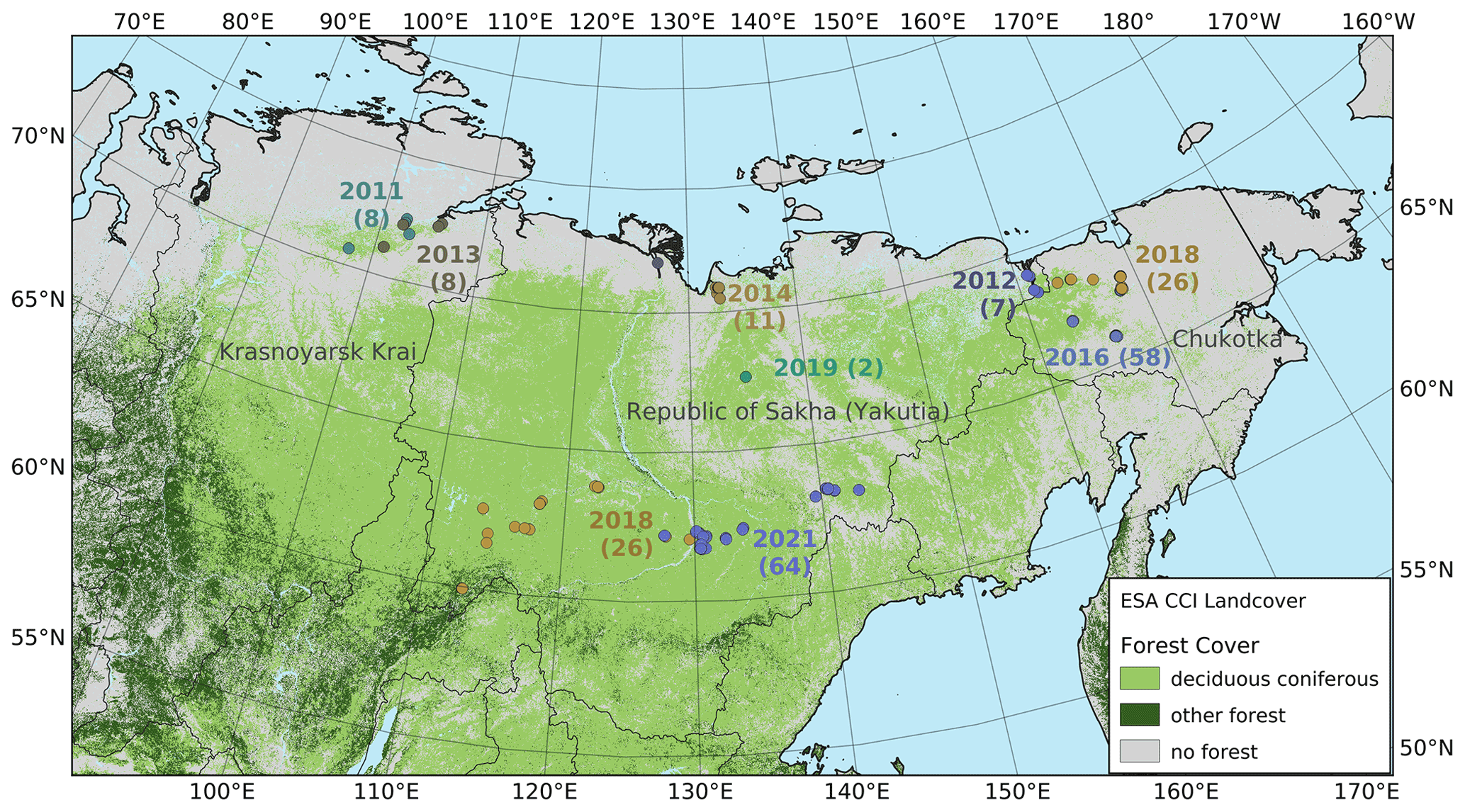
Figure 1 The vegetation in the larch-dominated forests of northeastern Russia. Numbers indicate the year and the number of vegetation plots on each expedition.

Figure 2 The climate on the plots according to CHELSA (Climatologies at high resolution for the Earth’s land surface areas) data. Mean January temperature is shown on the y axis, mean July temperature is shown on the x axis, and mean annual precipitation as coloured dots.

The sites at which the surveys were performed were chosen beforehand, with the consideration of remote sensing data. The goal was to cover a wide range of conditions such as tree cover percentage and reflectance values in the region of each expedition. The exact positioning of the survey plot was finalized on site, with the aim to have each plot representing a homogeneous vegetation type. Not all vegetation survey plots contain forest or even single trees; some were used to record ground vegetation and tree recruitment, while taller trees were absent.

The geographic coordinates of the plot centre were recorded with a GPS device, using the datum WGS 84 (World Geodetic System). Plots were either rectangular or circular. Rectangular plots were more commonly used in the tundra–taiga ecotone. They would typically be squares of 20 m × 20 m, but their size was sometimes increased in areas with very few trees per hectare or decreased in size if the vegetation or topography demanded it. A grid of 2 m × 2 m was laid out over the plot in order to locate trees precisely inside of it. In a rectangular plot, every tree was recorded in detail and the following variables were noted: species, height, vitality estimate (on a discrete scale, from very vital, vital, mediocre, low, and very low to dead), growth form, basal diameter, diameter at breast height (DBH), maximum crown diameter, and the smaller crown diameter, which was measured perpendicular to the maximum.

Circular plots had a diameter of 15 m, except for occasions in which the forest was too dense to record all trees in this range; in these cases, the diameter was reduced to 10 m. Of the trees in the circular plot area, a minimum of 10 trees was chosen for the detailed inventory as above. The goal was to choose 10 trees per species so that they covered the entire range of height and diameter variation present on the plot. If there were more than two species, then the number of chosen trees per species was reduced due to time constraints, with the focus on coniferous trees. After making the detailed inventory of the chosen trees, all trees on the plot were recorded, noting only the species, estimated height, and general remarks, for example, whether the tree had low vitality, was dead, inclined, or not of upright growth form. Based on this, the variable growth type can take the values of tree (T), shrub (S), tree lying (TL for lying deadwood), multistem (M, if several shoots emerged from the same base), and krumholz (K). Larix can occur both in the tree form and in the krumholz form. The criterion for the latter is the lack of a straight, upright stem (Kruse et al., 2020b). The variable survey protocol tells us if the tree was recorded on a rectangular plot (PLOT), outside of a plot (EXTRA), or on a circular plot. In the latter case, the variable takes the value PLOTHEIGHT, if only height was measured, and CIRCLEPLOT, if it is the detailed inventory. Those trees were recorded twice, with different IDs, i.e. once as PLOTHEIGHT and once as CIRCLEPLOT. In order to avoid duplicate entries, the data set was later split up into two tables, so that, within each table, any tree would only be mentioned once.

Tree height was measured with a clinometer for some trees and, for others, visually estimated by making a comparison with the measured trees or objects of known height. According to experience, the error in this method was below 10 % for smaller trees or below 1 m for larger ones. Generally, all trees at least 40 cm in height were measured. Additionally, for many plots along the treeline, where recruitment was the focus of the research, smaller individuals were recorded on subplots. Stem diameters were measured either with a measuring tape (as circumference) or a calliper, recording the basal diameter just above the root collar and DBH at 1.3 m above the ground. Crown diameters were estimated from below, with the help of ground measurements using a measuring tape.

Parts of the data set presented here has already been published in other data publications and are available individually:

• Wieczorek et al. (2017) (including data of the 2011 and 2013 expeditions) at https://doi.org/10.1594/PANGAEA.874615,

• Kruse et al. (2020a) at https://doi.org/10.1594/PANGAEA.923638, and

• van Geffen et al. (2021) at https://doi.org/10.1594/PANGAEA.932821.

2.3 Processing of the data

In the two tables of the tree database, i.e. tree heights and tree measurements, every entry contains information about one tree. Some processing was done prior to the analysis to derive variables that were not present in the original data set. The entire list, displaying which variables were recorded directly on site and which were derived from other measurements, can be found in Appendix B.

The species of each tree was recorded differently, depending on the surveyor. This led to differences in the naming convention, for example, Betula pendula on some plots and Betula spec. on others. Therefore, the 23 taxa entries were harmonized into 10 species groups, as identified by the genus name. The species Larix gmelinii and Larix cajanderi were grouped together in the species group Larix. An exception is the genus Pinus, where Pinus pumila (Pall.) Regel was excluded from the Pinus group due to its shrub-like growth form.

Height was recorded for all trees, but diameters only for selected ones, and the existing diameters were used to calculate allometries from which the diameters were then reconstructed from the height for those trees where they were not measured. For each species group, a power function of the form

$$D_{\mathrm{BS}}=a_{\mathrm{1}}\cdot H^{a_{\mathrm{2}}}$$

was fitted with the least squares method (where D_BS is the diameter at base, H is the height, and a₁ and a₂ are the optimization coefficients). For diameter at breast height (D_BH), the function is as follows:

$$D_{\mathrm{BH}}=a_{\mathrm{1}}\cdot (H-\mathrm{1.3}{)}^{a_{\mathrm{2}}}.$$

Initial analyses with this function revealed that the diameter estimations were biased on some plots. On densely forested plots, trees tended to have smaller diameters at the same height compared to sparsely forested plots, especially in the lower half of the height range. As the power functions computed for the different stand density groups (measured in trees per hectare) differed both in exponent and in factor, we used the adjusted power function,

$$D_{\mathrm{BS}}=(a_{\mathrm{1}}+a_{\mathrm{3}}\cdot S)\cdot H^{(a_{\mathrm{2}}+a_{\mathrm{4}}\cdot S)},$$

where the stand density S was computed from T_ha, the number of trees per hectare, as follows:

$$S=max\left({\log }_{\mathrm{10}}\right(T_{\mathrm{ha}}),\mathrm{2})).$$

The formula for D_BH was analogous, replacing H with (H−1.3). The latter formulas were only applied to the species group Larix, as all other species were not present on enough different plots to prevent overfitting. For all other species groups, the former, simpler formulas were used.

Having thus obtained the variables for the predicted diameter at base (DBS) and predicted DBH for all trees, it was possible to calculate further metrics, including the basal area (BA),

$$\mathrm{BA}={\displaystyle \frac{\mathit{\pi }}{\mathrm{4}}}{D_{\mathrm{BH}}}^{\mathrm{2}},$$

and stem volume (V), which was obtained using the Smalian volume formula (Cailliez and Alder, 1980) for trees taller than breast height,

$$V={\displaystyle \frac{{D_{\mathrm{BS}}}^{\mathrm{2}}+{D_{\mathrm{BH}}}^{\mathrm{2}}}{\mathrm{2}}}\cdot {\displaystyle \frac{\mathit{\pi }}{\mathrm{4}}}\cdot \mathrm{1.3}+{\displaystyle \frac{{D_{\mathrm{BH}}}^{\mathrm{2}}}{\mathrm{2}}}\cdot {\displaystyle \frac{\mathit{\pi }}{\mathrm{4}}}\cdot (H-\mathrm{1.3}),$$

and for trees smaller than breast height, respectively, and

$$V={\displaystyle \frac{{D_{\mathrm{BS}}}^{\mathrm{2}}}{\mathrm{2}}}\cdot {\displaystyle \frac{\mathit{\pi }}{\mathrm{4}}}\cdot H.$$

After calculating these variables for the individual trees, the database was split up into two tables to avoid a situation in which individual trees would appear twice in the same table under two different survey protocols. The table of tree heights includes all standing trees inside of the plots with heights from 0.4 m upwards. From the circular plots, the table includes only the PLOTHEIGHT measurements. The table of the tree measurements includes all other entries, including all CIRCLEPLOT and PLOT measurements, even though the PLOT measurements are also included in the table of tree heights. This was done so that all entries with diameter measurements would be included in the tree measurements table. Of the information in the tree heights table, several variables were aggregated at the plot level by calculating mean and selected quantiles of height in addition to the sum of the basal area and stem volume. The latter variables were then divided by the plot area to obtain the respective values per hectare.

Another measure we calculated for the height distributions of each plot is the Gini coefficient (Gini, 1912). It ranges between 0 and 1, assuming a value of 0 if all trees have the same height and approaching 1 if there are a few very big trees alongside many very small ones. Let h_i be a collection of height measurements in ascending order and i in $\mathit{\{}\mathrm{1},\mathrm{\dots },n\mathit{\}}$. Then, the Gini coefficient is defined as follows:

$$\mathrm{1}-\mathrm{2}{\displaystyle \frac{{\sum }_{i=\mathrm{1}}^n(h_i\cdot (n-i+\mathrm{0.5}\left)\right)}{{\sum }_{i=\mathrm{1}}^n(h_i\cdot n)}}.$$

2.4 Data products for comparison

In the study, we used several gridded, mostly remote-sensing-derived data products on climate, biomass, height, forest cover loss, and stand age to compare with and relate to the forest inventory.

2.4.1 Climate

CHELSA (Climatologies at high resolution for the Earth’s land surface areas; Karger et al., 2017, 2021) is a global raster data set containing many different variables, like monthly mean temperatures and precipitation sums, and several different bioclimatic variables. This study uses the temperature means for the months of January and July, the sum of the monthly precipitation, and the growing degree days above 0 ^∘C (GDD0).

All values are means for the period 1981–2010, with a spatial resolution of 30 degree seconds, which is less than 1 km.

2.4.2 Forest biomass

The GlobBiomass data set (Santoro et al., 2018, 2021) covers the Earth's land surface with a pixel size of 1 ha. It provides values for the aboveground biomass (AGB) and growing stock volume (GSV) for the year 2010, in addition to the standard errors derived from satellite-based synthetic aperture radar, and an extensive set of ground measurements. The authors note that their data set is not precise at the pixel level but is better when aggregated over larger areas.

2.4.3 Forest height

The forest canopy height product (Simard et al., 2011) is a raster data set with a resolution of 1 km². It estimates the maximum canopy height in each pixel from the Geoscience Laser Altimeter System (GLAS) satellite-borne lidar, using additional data about climate, elevation, and canopy cover. All values are for the year 2005.

2.4.4 Tree cover loss

We used the tree cover loss product from the Global Forest Watch project (Hansen et al., 2013), which is based on yearly observations of Landsat images (30 m resolution). The project publishes various related data sets, e.g. a product about forest cover gain, and most products are updated regularly. The tree cover loss product detects, for each pixel, if it has been converted from containing tree cover (yes/no) to not containing tree cover in the time from 2000 to 2019. It assigns the year of the loss to a given pixel or 0 if no loss has taken place since the year 2000.

2.4.5 Siberian larch stand age

The Distribution of Estimated Stand Age Across Siberian Larch Forests (Chen et al., 2017) is related to the former data set and is also mainly based on Landsat images with 30 m resolution. It incorporates some more analysis to detect stand-replacing forest fires, but it only covers a part of eastern Siberia, including 54 of our vegetation survey plots, and spans the years 1989–2012. For every pixel, it gives the age of the forest stand as if it has experienced a stand replacing fire since 1989, a value of 100 if there has been no fire between 1989–2012, or no data if the pixel does not contain larch forest.

2.5 Analysis methods

The remote sensing products that were used all consisted of raster data. The values at the locations of the plot centres were extracted using QGIS 3.16 (QGIS, 2021).

From the CHELSA climate data set, four variables were chosen for further analyses, namely annual precipitation sum (Prec.), January mean temperature (T01), July mean temperature (T07), and growing degree days above 0 ^∘C (GDD0). Univariate linear regressions were calculated between every single variable and four forest inventory variables.

To compare the GlobBiomass product and the forest height product with our data, linear regressions were calculated between the remote-sensing-derived variables and suitable variables of our forest plot data, like stem volume.

We compared the quotient of the living basal area over the total basal area for plots with recent tree cover loss and plots without recent tree cover loss as assessed by a two-sided t test. All analysis was performed in R 4.1.0 (R Core Team, 2021).

3 Results

3.1 Description of the data

3.1.1 Descriptive statistics

The tree database comprises 42 675 entries, describing 40 289 trees. This is due to the fact that, on circular plots, the trees that were subject to detailed inventory are also recorded again in the height-only inventory. Of these, 33 513 individuals were used for aggregation at the plot level. The rest were excluded for being smaller than 40 cm, because such trees were not recorded on every plot, or for being located outside of the vegetation plots listed in the plot database.

The plot database includes 226 vegetation plots, of which 162 contain trees taller or equal to 40 cm. Of the 40 289 trees, 4660 (11.6 %) were dead and 35 629 (88.4 %) living at the time of recording. All entries in the tree database have a recorded height, which ranges up to 28.5 m. The species is recorded for all but 31 entries. The most frequent species are Larix cajanderi (44.4 % of database) and Larix gmelinii (25.7 %). The two Larix species never occur together on the same plot. Other frequent taxa are Betula pendula Roth (13.9 %), Picea obovata Ledeb. (5.8 %), Pinus sylvestris L. (5.0%), and the genus Salix spec. (3.2 %). Among the less frequent taxa are Populus tremula L., Alnus spec., Pinus pumila Regel, Pinus sibirica Du Tour, and Abies sibirica Ledeb.

Values for basal diameter are present for 2583 entries. They range from 0 to 97.7 cm, with the median at 6.99 cm and mean at 11.08 cm. For diameter at breast height (DBH), there are 2095 values in the data set, almost all of which are trees for which the basal diameter is also given. DBH is almost always lower than basal diameter, on average by the factor 0.628. DBH ranges up to 71.6 cm, with the median at 6.4 cm and mean at 9.02 cm. Maximum crown diameter and smaller crown diameter (measured perpendicular to maximum) are given for 2079 entries and range from 0 to 16 m. The quotient of the two diameters is, on average, 0.81. Tree crown area, which is the product of the two values and the factor $\frac{\mathit{\pi }}{\mathrm{4}}\cdot \frac{\mathrm{1}{\mathrm{m}}^{\mathrm{2}}}{\mathrm{10}\mathrm{000}{\mathrm{cm}}^{\mathrm{2}}}$ is, on average, 4.77 m², with a median of 1.43 m².

3.1.2 Diameter–height allometry

The power function allometries for the different species differ notably, as can be seen in Fig. 3. The basal diameter of birches (Betula), for example, is obtained from height with an exponent of a₁ = 1.15 and a factor of a₂ = 0.91, while for Abies, the exponent is a₁ = 0.66 and the factor is a₂ = 2.69. The genus Populus differs strongly from the other species groups, with an exponent of a₁ = 2.29 and a factor of a₂ = 0.06. In the DBH-model Populus differs remarkably from the others, too, even if not that strongly. All factors and exponents are displayed in Appendix C.

The graphs in Fig. 3k and u show the diameter–height allometries for the genus Larix when taking into account the number of trees per hectare. When tree measurements are grouped by stand density, the resulting power functions differ by more than the respective standard errors for the coefficients, especially for heights between 4 and 12 m, where a higher number of trees on the plot have smaller diameters.

Figure 3 Diameter at base (DBS; left) and diameter at breast height (DBH; right) against the height per species. Power function allometries per species are shown. Panels (k) and (u) show Larix only, coloured by trees per hectare. The regression lines illustrate the allometry for three different stand densities (300, 3000, and 30 000 trees per hectare), while, in the actual allometric formula, the stand density is a continuous variable.

3.1.3 Height distributions

Tree heights show a nearly exponential distribution, with the exception that values from approximately 15 m upward occur slightly more frequently than expected under an exponential distribution (Fig. 4). However, at the level of individual plots, the distribution patterns vary widely. This can be seen in Fig. 5. Although the tree heights on plot EN21-260 are close to an exponential distribution, suggesting a continuous recruitment rate, in EN21-253 the larger trees are overrepresented. Plot EN21-230 is missing the smallest cohort, and plot EN21-246 is an example of dense regrowth after a stand-replacing fire, where older trees taller than 7 m are absent. Plot EN21-226 is dominated by a cohort of middle-sized trees, lacking both small and very large ones. In EN21-219, some large and many small individuals are present, while medium-sized ones are missing.

The Gini coefficient is normally distributed with a mean of 0.363 and standard deviation of 0.123. Plot EN21-258 is an example of a plot with a high Gini value (0.679), and plot EN21-226 is at the lower end, with a Gini coefficient of 0.166. The Gini coefficients are negatively correlated with the geographic latitude of the plot (Fig. 5). The linear regression has a p value of 0.021, and R² = 0.33.

Figure 4 Height distribution of all trees on plots.

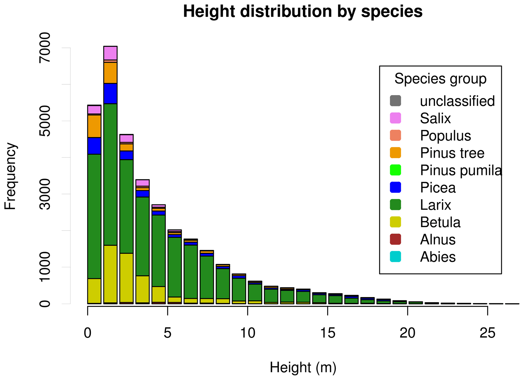
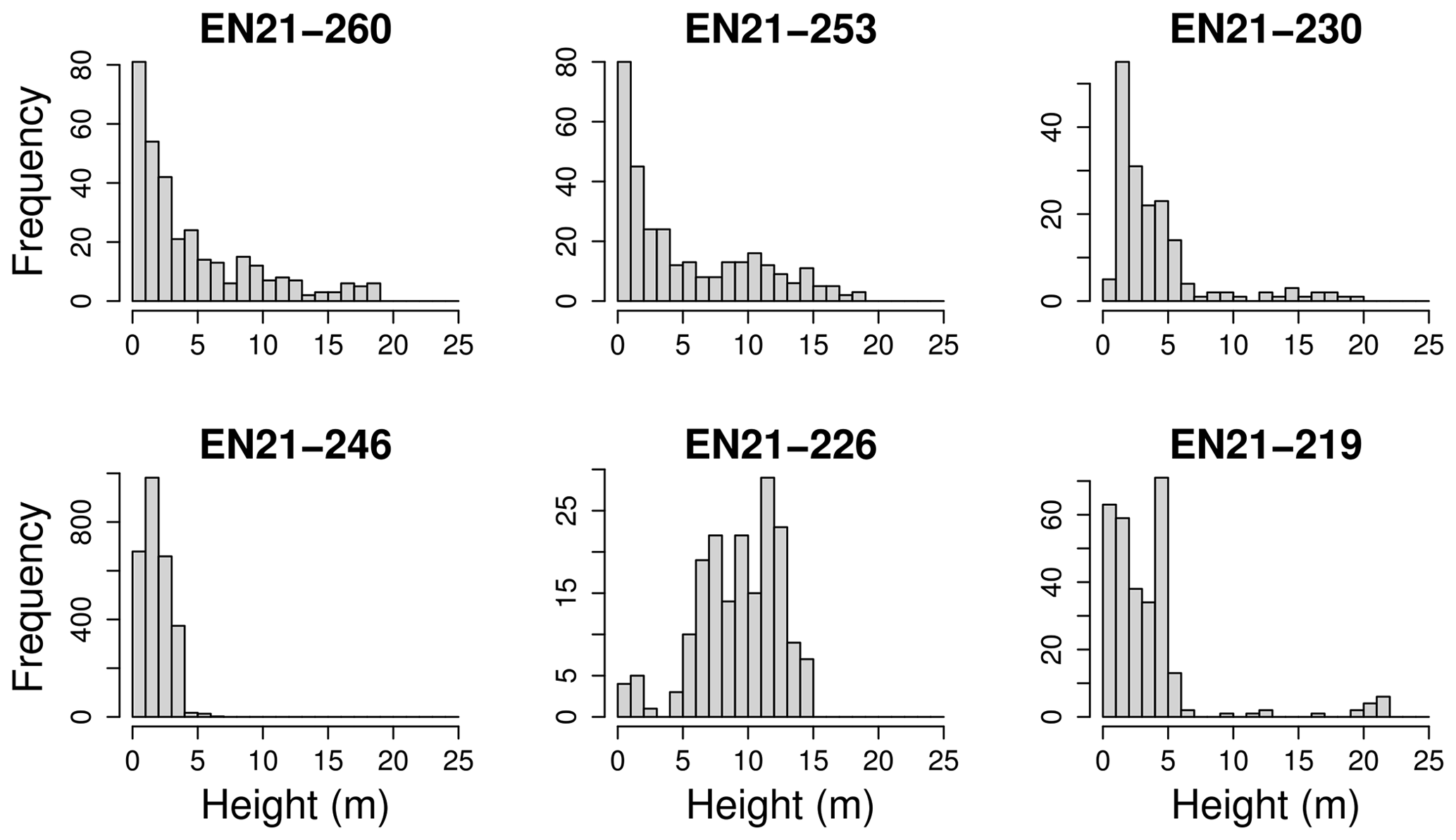
Figure 5 The height classes among all species for six different plots of the Yakutia 2021 expedition, which were chosen as examples for differing height distributions.

Figure 6 Gini coefficients for height against latitude, coloured by most frequent species on plot. (Plots with more diverse height distributions have higher Gini coefficients.)

3.1.4 Species distribution

In accordance with the known ranges of the different species, we observe that species diversity tends to be higher on the plots in central and western Yakutia, which experience warmer summers and longer growing seasons than the plots near the northern treeline. All plots north of 70^∘ N have only one species (larch), while, for the plots south of 65^∘ N, there are, on average, 3.11 species, with a maximum of 9 tree species from 7 species groups.

The species Pinus sylvestris, Picea obovata, Abies sibirica, Ulmus spec., and Populus tremula only occur on the plots south of 65^∘ N, with a July temperature of at least 17 ^∘C. More predominant among the southerly plots are Betula pendula and Alnus spec., but they are also found at one and three plots, respectively, in Chukotka. The taxa Pinus pumila and Salix spec. occur frequently between 65 and 70^∘ N. Of the plots with trees, all but one have Larix individuals. For the plots to the west of 130^∘ E, it is L. gmelinii, and for the plots east thereof, it is L. cajanderi.

3.2 Remote sensing products as predictors

3.2.1 CHELSA Climate

The climate on the plots is strongly continental (see also Fig. 2), with mild to warm summers and extremely cold winters. The length of the growing season is between 63 and 132 d, and the GDD0 ranges from 565 to 1974.

Weak correlations between four climate parameters (precipitation, January temperature, July temperature, and GDD0) and four forest structure parameters (mean height, log₁₀ (number of trees per hectare), basal area per hectare, and stem volume per hectare) are found (Fig. 7). The climate variables mean that the January temperature (T01) and precipitation have very low correlation coefficients with all forest metrics. The correlations between T01 and the forest metrics are even negative, although R² values are close to 0. Mean July temperature (T07) and GDD0 are more strongly correlated with several forest structure parameters, but the strength of the correlation is only intermediate and does not exceed R² = 0.321 in any combination. The predictor variables are also correlated among each other, especially T07 and GDD0 (R² = 0.993; all correlations are shown in Appendix D).

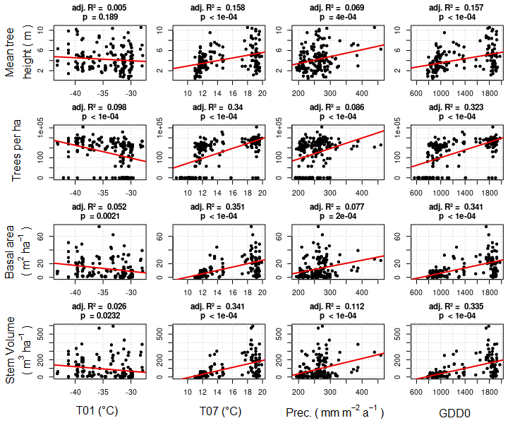
Figure 7 Comparison of forest inventory variables with climate variables. Linear regression lines are given in red.

3.2.2 GlobBiomass

The two leading variables from the GlobBiomass data set – aboveground biomass (AGB) and growing stock volume (GSV) – are themselves strongly correlated (R² = 0.989 over all plots). Therefore, we focus on just one of them – GSV – which can be derived from our data with more confidence, since we did not measure the wood density and biomass expansion factors.

Remote-sensing-derived GSV and inventory-derived GSV follow the same tendency (correlation with R² = 0.49 and residual standard error 79.9; Fig. 8). But, for some plots, the two values differ by more than an order of magnitude.

Figure 8 Stem volume calculations plotted against growing stock volume (GSV) from the GlobBiomass data set. (a) Linear scale. (b) Logarithmic scale, with zeroes removed.

3.2.3 Forest height

The values of the Simard et al. (2011) data are 0 (no forest) or have integers between 11 and 27 for the forest height in metres. On 125 of the plots, they record a value of 0, while we actually encountered trees on 60 of these plots in our inventory. A linear correlation between the Simard et al. (2011) canopy height and the maximum tree height on the plot (Fig. 9) has an intercept of 8.55, a slope of 0.298, and R² = 0.20. Other metrics, such as the 98th, 90th, or 75th percentiles of the observed tree height, have even less correlation (see Appendix E).

Figure 9 Highest tree of the inventory plots plotted against canopy height, according to the Simard et al. (2011) data set. Linear regression line in red.

3.2.4 Forest loss

The data set for the Stand Age of Siberian Larch Forests by Chen et al. (2017) has data for 54 of our vegetation plots and finds that 6 plots have experienced stand-replacing events between 1989 and 2012. The Hansen et al. (2013) data set covers a wider area and different time range. However, there are five plots for which they detect forest loss in times and places where Chen et al. (2017) find that the stand age is at maximum. We encountered clear signs of recent disturbance in the vegetation at only 50 % of the plots where either of the data products detected forest loss.

The average quotient of the basal area of living trees to overall basal area is higher for the plots without disturbance than for the plots with forest loss, according to the Hansen et al. (2013) data set, which shows that there is more standing deadwood on plots with forest loss (Fig. 10). Although a t test finds that the two groups differ very significantly (p =$\mathrm{4}\times {\mathrm{10}}^{-\mathrm{6}}$), we see that there are also individual disturbance plots in which dead trees do not constitute a relevant number for the basal area. On most of these, field observations did not find signs of recent disturbance, except for one plot where the natural succession was at a pioneer stage.

Figure 10 Living wood volume compared to overall wood volume. Plots with recent forest loss are marked red.

4 Discussion

4.1 Relevance of the data set

The data we present in this study are unique in their extent for the regions they cover. Schepaschenko et al. (2017) have compiled a vast number of forest inventories in Eurasia, but their coverage of our study region is sparse. For example, they include no data from Chukotka and the Kolyma area, where our data set has 91 plots. The same is true for the validation data set used by Yang and Kondoh (2020), who have only one location within our area of interest from the more than 400 literature sources they reviewed. This shows the lack of forest inventories from northeastern Siberia, which our data set aims to mend.

4.2 Validity of methods

The fieldwork was carried out according to scientific standards. Tree height was chosen as the leading variable because it is easy to have an overview of sparse stands, and it generally correlates well with other variables (stem diameter and biomass). Diameter at breast height (DBH), even though it is more commonly used as a predictor, is more laborious to determine for trees in sparse stands with low crowns. With frequent clinometer measurements, we assured precise height estimations, and the remaining errors can be expected to average out over the high number of observations, which were easily obtained due to the efficiency of the method. Drawbacks coming with this method are explained in the following. Since the diameter is only predicted from height, errors from this prediction propagate into derived variables like basal area and stem volume. And the initial measurement error, even if small, propagates along the same way. This error was not quantified systematically.

The correlations of the forest metrics with climate variables (Sect. 3.2.1) cannot be generalized because the distribution of the plots is not representative of the area. Even though the survey plots in each region cover the entire range of vegetation in any given zone, they are not weighed according to the occurrence of the vegetation type they represent. However, the relationships can still give us some idea of the general behaviour of the variables.

4.3 Tree species and heights distribution

We observe a higher species diversity in the more southerly stands which experience longer, warmer growing seasons. This is in accordance with the expectations and the known ranges of the observed tree species (Kuznetsova et al., 2010).

It is uncommon in the literature to record height distributions, but methodological analogues are age class or diameter distributions, which can be used to show recruitment patterns, e.g. Lin et al. (2005). While the close-to-exponential distribution of tree height suggests a continuous recruitment rate and continuous mortality throughout the age classes, a closer look at individual tree stands shows that they differ strongly from each other. This suggests that recruitment patterns are only continuous at the landscape scale, but discontinuous at the local scale, which is consistent with the well-known fact that stand-replacing fires regularly rejuvenate forests in the permafrost ecosystems of our research area (Kharuk et al., 2011).

4.4 Allometries

We see that the tree species have very different allometries. This may be partially due to the fact that they are actually different and partially due to the random effects of the plots and the small sample sizes for some species groups, like Abies (10 measurements for DBS) and Populus (27). The species groups with more than 100 measurements (Betula, Larix, Picea, and Pinus) have smaller differences among each other in the allometry coefficients. There is little literature with which to compare our results because the diameter, and not height, is commonly used as a predictor variable, as in Alexander et al. (2012) and Delcourt and Veraverbeke (2022), who both model biomass from diameter. We still chose to use height as the principal variable, as it is very easy to estimate in sparse forest stands. Nevertheless, using height as a predictor, Kajimoto et al. (1999) find a similar exponent for the Larix gmelinii stem weight as we found for volume.

4.5 Comparison of inventory and remote sensing

We find, for the examined remote sensing products, that predicting forest statistics on the plot base results in large errors. There are various factors that can lead to such a mismatch, as discussed by Houghton et al. (2007). Imprecision in the field measurements or the data processing may play a role (Picard et al., 2015). But likely another relevant factor is the coarse resolution of the remote sensing data, alongside the heterogeneity of the landscape on the scale between plot size and pixel size. The Simard et al. (2011) canopy height product, for example, has a resolution of 1 km², which is more than 1000 times our average vegetation plot size. Therefore, it cannot capture differences in canopy height below the kilometre scale, even though many landscape elements are smaller than this. This mismatch in resolution becomes especially relevant in the forest tundra, where the sparsity of the stands makes them difficult to detect in satellite images (Ranson et al., 2004; Montesano et al., 2016).

Another issue may be the lack of calibration of the remote sensing data sets, especially in the poorly researched area of northeastern Siberia. Zhang et al. (2019), who investigated numerous remote-sensing-based forest data sets, suggest that most of them suffer from a lack of validation and ground-truthing. Furthermore, Yang and Kondoh (2020) investigated the Simard et al. (2011) data set, and they find that it generally overestimates small canopy heights and underestimates large ones. When assessing the reliability of their biomass data product, Santoro et al. (2018, 2021) note that the relative AGB standard error in eastern Siberia is among the highest in the world, indicating a large uncertainty for this region.

A different source of error is the temporal mismatch between the acquisition of the inventory data and the remote sensing images. This varies throughout our data set, as the expeditions span a time range of 10 years, which is not accounted for in the comparisons, except for the comparison with the forest loss data sets. However, in the time ranges considered here, we can assume that the differences in variables such as stand height and growing stock volume are small, due to the very low growth rates of the forests in the region (Kajimoto et al., 2010). Only disturbances, such as wildfires and insect pests, could create large changes in the growing stock in a relatively short time.

We expect that all forest loss in our area is due to fire, as we did not find any signs of deforestation due to human activities on any of the surveyed plots. While the analysis of the forest loss data set led to the expected result that the plots with recent forest loss tend to have lower fractions of living basal area, it is still surprising that we saw some plots that were supposedly affected by forest loss, and thus by fire, with a large part of the stand alive, both in absolute and relative terms. This may be because many forest fires in Siberia are low-intensity fires (Ponomarev et al., 2022) which are detected as burned forest in 1 year, even though a large part of the trees recovers by the following year. Revisiting some of our survey plots in the future may help to improve the understanding of this topic.

4.6 The influence of climate on forest metrics

We find that the climate explains many of the quantitative forest metrics, albeit to a limited extent. Forest metrics such as basal area and stem volume are positively correlated with summer temperatures and growing degree days. However, the observed correlations are quite weak, and the range of the forest metrics is large. This suggests that the forest we observed is spatially heterogeneous and depends on properties which vary on smaller spatial scales than the climate.

It is counterintuitive that the investigated forest metrics are negatively correlated with January temperature in our data set, but it can be explained by the January temperature being negatively correlated with the July temperature (see Appendix D) and length of the growing season (R² = 0.31; slope is −0.107), which is another bioclimatic variable from the CHELSA data set. The plots near the Arctic Ocean have a less continental climate, meaning that they tend to have both milder winters and cooler summers than the more southerly ones. Thus, we cannot conclude that colder winters are favourable for forest growth.

There is scarcely any correlation between our observed forest metrics and precipitation, which suggests that water availability is not a limiting factor for forest growth in northeastern Siberia. Sugimoto et al. (2002) support this hypothesis by pointing out that larch forests in these regions have a good supply of water from snowmelt, rain, or thawing permafrost, depending on the weather in any given year. Opposed to this, Kharuk et al. (2019), who investigated a larch forest on the central Siberian Plateau, report that, since the 1990s, growth has been diminished by drought stress and extreme events, which are increasing under climate warming, like the 2020 Siberian heat wave (Collow et al., 2022). Kropp et al. (2017) and Walker et al. (2021) support findings that water availability is a limiting factor for Larix cajanderi.

4.7 Outlook

The analyses performed in this study do not exhaust the possibilities offered by this data set and serve purely to present the data. The fact that individual trees were measured, and related to the inventory plots, make it a very versatile data set. Some variables that were taken in the inventory can be analysed further. In particular, the crown diameters and crown base have not been assessed as yet. The forest inventory could be related to other, still unpublished data collections from the same expeditions, such as the projective crown cover estimations, ground vegetation surveys, soil profiles, genetic samples, stem increment cores, and stem discs. These additional samples were not collected for all individuals, but they could at least be related to a portion of the forest inventory data. Also, for some of the more recent expeditions, drone-based photogrammetric and lidar point clouds exist (e.g. SiDroForest) and could provide insight into the heterogeneity of the landscape and bridge the gap between survey plot size and pixel size of satellite-derived data. Furthermore, these centimetre-resolution point clouds are capable of capturing single tree measurements and bringing them to the landscape level. A different way to fill this gap and improve the predictions of the state of remote forests is with remote sensing products at a higher resolution, such as the boreal forest canopy height data set in connection with Potapov et al. (2020). They published a global canopy height data set with 30 m resolution for the tropical and temperate zones of the world, and the data for the boreal regions are expected to be released soon.

Our data set can also be used to calibrate and improve current and future remote sensing products. For this purpose, researchers can rely on the individual tree measurements, such as height, and on metrics aggregated at the plot level. The data set can serve to calculate or improve allometries for the investigated taxa, especially the two eastern Siberian larch species of Larix cajanderi and Larix gmelinii.

5 Data availability

The data are available at https://doi.org/10.1594/PANGAEA.943547 (Miesner et al., 2022).

6 Conclusions

We presented and analysed a data set resulting from forest inventories in various regions of northeast Siberia. A subset of the entries includes diameter measurements and height measurements, whereas the majority only includes height. Therefore, we computed diameter–height allometries, which are reasonably accurate overall but show a bias for some plots. It proved difficult to predict forest metrics at the plot level, for example, stem volume and basal area, from a selection of remote sensing products, as these were not strongly correlated. Among the climatic variables taken from the CHELSA data set, the mean July temperature is one of the best predictors, along with GDD0 and length of growing season, while the mean January temperature and precipitation proved almost insignificant. The GlobBiomass data set and the Simard et al. (2011) forest height product are correlated with the volume and height measurements on the survey plots but unsuitable for predicting the latter on a small scale. The data sets used for forest age and disturbance often differ from both each other and the observations made in the field. This leads us to conclude that, even in our time of widely available global remote sensing data sets, field measurements like the ones presented here are still vital for the understanding of remote ecosystems such as the larch-dominated forests of northeast Siberia.

Appendix A: Overview over all vegetation plots

Table A1 Overview over all vegetation plots. NA: not available. n/a: not applicable.

Appendix B: Overview over all variables

Table B1 List of all variables of the tree database. The spelling, capitalization, grammar and units reflect the original database.

Table B2 List of all variables of the plot database. The spelling, capitalization, grammar and units reflect the original database.

Appendix C: Coefficients of diameter–height allometries

Allometries were calculated to obtain the diameter from the height of the tree with the following formula:

$$D=(a_{\mathrm{1}}+a_{\mathrm{3}}\cdot S)\cdot H^{(a_{\mathrm{2}}+a_{\mathrm{4}}\cdot S)},$$

where D is the diameter in centimetres. H is the height, and S is the stand density, which is obtained from the number of trees per hectare (T_ha) as follows:

$$S=max\left({\log }_{\mathrm{10}}\right(T_{\mathrm{ha}}),\mathrm{2})).$$

The coefficients a₁, a₂, a₃, and a₄ resulting from fitting with the least squares method are shown in Tables B1 and B2.

Table C1 Coefficients for diameter at base allometries.

Table C2 Coefficients for diameter at breast height allometries.

Appendix D: Correlation matrix of climate variables

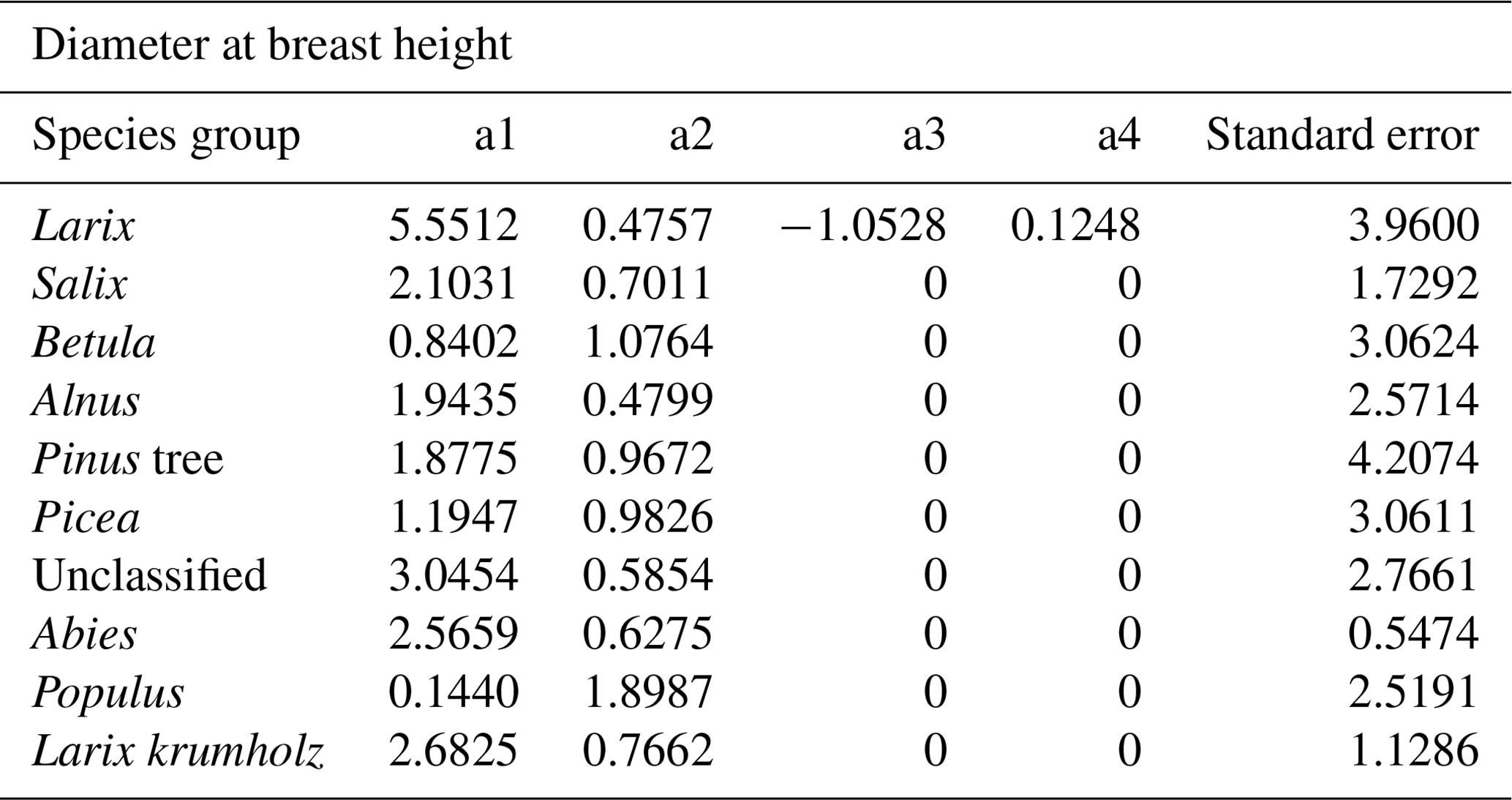
Table D1 Correlations between the four climate variables, namely the January temperature (T01), July temperature (T07), annual precipitation (Prec.), and growing degree days above 0 ^∘C (GDD0), from the CHELSA data set at the locations of our plots, calculated using the R function cor().

Appendix E: Correlation coefficients for forest canopy height

In Sect. 3.2.3, linear correlations were calculated between the Simard et al. (2011) forest height product and different forest metrics (heights in metres), with the results shown in Table E1.

Table E1 Correlation coefficients for forest canopy height. Adj. R²: adjusted R².