the Creative Commons Attribution 4.0 License.
the Creative Commons Attribution 4.0 License.
 | 20 Dec 2022
WaterBench-Iowa: a large-scale benchmark dataset for data-driven streamflow forecasting
Ibrahim Demir
Bekir Demiray
Muhammed Sit
This study proposes a comprehensive benchmark dataset for streamflow forecasting, WaterBench-Iowa, that follows FAIR (findability, accessibility, interoperability, and reuse) data principles and is prepared with a focus on convenience for utilizing in data-driven and machine learning studies, and provides benchmark performance for state of art deep learning architectures on the dataset for comparative analysis. By aggregating the datasets of streamflow, precipitation, watershed area, slope, soil types, and evapotranspiration from federal agencies and state organizations (i.e., NASA, NOAA, USGS, and Iowa Flood Center), we provided the WaterBench-Iowa for hourly streamflow forecast studies. This dataset has a high temporal and spatial resolution with rich metadata and relational information, which can be used for a variety of deep learning and machine learning research. We defined a sample benchmark task of predicting the hourly streamflow for the next 5 d for future comparative studies, and provided benchmark results on this task with sample linear regression and deep learning models, including long short-term memory (LSTM), gated recurrent units (GRU), and sequence-to-sequence (S2S). Our benchmark model results show a median Nash-Sutcliffe efficiency (NSE) of 0.74 and a median Kling-Gupta efficiency (KGE) of 0.79 among 125 watersheds for the 120 h ahead streamflow prediction task. WaterBench-Iowa makes up for the lack of unified benchmarks in earth science research and can be accessed at Zenodo https://doi.org/10.5281/zenodo.7087806 (Demir et al., 2022a).
- Article
(1641 KB) - Full-text XML
- BibTeX
- EndNote


Deep learning, a set of algorithms based on artificial neural networks (ANN) for supervised and unsupervised modeling, has been widely used and recognized as a powerful approach within many scientific disciplines for technological and predictive progress (Goodfellow et al., 2016). As conventional machine learning techniques were deemed limited in learning the representations of high-dimensional datasets from their raw form, by providing universal approximator models (Cybenko, 1989; Hornik et al., 1989; Leshno et al., 1993), deep neural networks increased scientists' ability to model both linear and non-linear problems without time-intensive data engineering processes by domain experts (LeCun et al., 2015). Deep learning's predictive modeling capabilities have led to improvements in various fields, including image recognition and synthesis (Demiray et al., 2021), speech recognition, language modeling, and time-series prediction.
Flooding is a significant concern for many areas in the world as it is on an upward trend due to climate change. The 1998 Bangladesh flood, the Iowa flood of 2008, and the 2013 North India floods show how catastrophic and both economically and psychologically devastating floods can be for populations in the respective regions. In order to maximize the preparedness for floods and minimize their effects after the disaster (Yildirim and Demir, 2021), weather and flood forecasting stands as a perennial research interest for hydrologists and data scientists. Streamflow prediction and runoff modeling are research efforts where the water from the land or channel over time is modeled and forecasted using previous data points for a location or nearby locations with similar characteristics. Although this effort is conventionally carried out with physically based models that require extensive computational (Agliamzanov et al., 2020) and data resources, it is critical for flood mitigation and decision support (Xu et al., 2020).
Being a time-series prediction task, in essence, flood forecasting takes advantage of the practicality and efficacy that deep learning brings to predictive modeling. Both time-series adaptations of deep learning models intended for natural language processing, and time-series focused deep neural network implementations make this possible by proposing methodologies that put the sequential nature of time-series datasets into good use. Recurrent neural network (RNN) architectures such as long short-term memory (LSTM) networks (Hochreiter and Schmidhuber, 1997), gated recurrent unit (GRU) networks (Chung et al., 2014), and attention-based sequence-to-sequence (S2S) networks (Vaswani et al., 2017) are pronounced starting point for deep neural network architectures for most time-series forecasting tasks.
Supervised learning, whether it be deep or not, is the most common form of machine learning (LeCun et al., 2015), and supervised learning tasks, such as flood forecasting, need a dataset of previously recorded or labeled entries for the task. That dataset typically consists of X and y values where X values are the input that the model expects, and y values are the output values the model returns. A supervised learning model is trained using a loss function that measures the similarity or difference of the y values from the dataset (actual y-values) and the outputs of the model (predicted ys). During a typical training process, predicted ys get closer to the actual ys in time, hence the name training. As a quintessential part of any supervised learning task, training neural network models on established datasets is common among deep learning practitioners and researchers (Goodfellow et al., 2016). For most tasks that deep learning researchers tackle today, there are vast amounts of benchmark datasets available freely for research. While computer vision datasets, such as Imagenet (Deng et al., 2009), Ms-celeb-1m (Guo et al., 2016), Adobe-240fps (Su et al., 2017), and Vimeo-90K (Xue et al., 2019) and similarly time-series datasets namely, automobile parts demand dataset (Seeger et al., 2016), electricity and traffic (Yu et al., 2016) have been widely used to test proposed neural network architectures, to the best of our knowledge. There are not many specific datasets that are published for geoscience studies (Ebert-Uphoff et al., 2017) and specifically for flood and streamflow forecasting.
The number of studies in hydrology and water resources, and particularly in flood forecasting that employ deep learning, has been gaining interest in the last several years (Sit et al., 2020). Flood forecasting studies in the literature, due to the aforementioned sequential nature, have vastly employed RNNs and LSTMs. Kratzert et al. (2018) utilized LSTM networks for daily runoff prediction using meteorological datasets. Furthermore, Kratzert et al. (2019) applied a similar approach for ungauged US locations. Bai et al. (2019) incorporated a stack autoencoder with LSTM for daily streamflow measurements from data for a week. Xiang et al. (2020) predicted the next 24 h of hourly streamflow rate by utilizing an encoder-decoder S2S neural network that also uses rainfall products. Xiang and Demir (2020), moreover, extended their study and developed a model that forecasts the hourly streamflow rate for the next 5 d using 3 d of historic data. They also incorporated upstream sensors into their proposed network. Using the same dataset, Xiang et al. (2021), explored the generalization of S2S encoder-decoder networks in flood forecasting. Sit and Demir (2019) predicted hourly sensor measurements for 24 h using data from the upstream sensor network and historic stage height measurements. Finally, Sit et al. (2021a), utilized graph neural networks for streamflow forecasting for a small watershed in Iowa. To sum up, deep learning models such as LSTM have been used in meteorology and hydrology studies of soil moisture modeling (Seeger et al., 2016), water table depth prediction (Zhang et al., 2018), rainfall runoff modeling (Hu et al., 2018; Kratzert et al., 2018), streamflow forecasting (Xiang et al., 2020). As represented in perspective studies (Reichstein et al., 2019), deep learning models such as LSTM can extract spatiotemporal features automatically to gain further process understanding of earth system science problems. Therefore, we pay great attention to the application of LSTM and its variant models in this research.
Most of the studies mentioned here acquired several raw data products, whether in terms of rainfall measurements, physical features of the studied area, or stage height, or discharge measurements, from authorities and build their own dataset benefiting from their expertise in the area. There are several datasets and benchmarks in other earth science studies, i.e., air quality forecast dataset, 3D cloud detection dataset, and LANL earthquake prediction dataset. One of the early user-friendly datasets in earth science is the Beijing PM2.5 data. It was published in 2017, and includes the hourly air quality PM2.5 data from the U.S. Embassy in Beijing and meteorological data from Beijing Capital International Airport. After the dataset was released, researchers developed different novel machine learning and deep learning models, including support vector machines (Zhu et al., 2018; Liu et al., 2019), recurrent neural networks (Athira et al., 2018), attention-based LSTM (Li et al., 2019), interpretable deep learning (Guo et al., 2018), hybrid deep learning (Du et al., 2019), convolutional networks (Tao et al., 2019), and stacked LSTM (Sagheer and Kotb, 2019) on this specific dataset. While knowledge of the application domain is essential to find scientifically robust ways to prepare the input data and to interpret the results of machine learning models, such knowledge is not always accessible to deep learning experts. If there are well-defined benchmark datasets with a clear description of the machine learning task to solve and have well-defined and domain-science informed evaluation metrics, then it becomes possible for non-domain experts to solve such challenges and introduce novel machine learning methods to the field. Furthermore, these papers used the same dataset and therefore the results are comparable. Thus, scientists could focus more on modeling and improving on the basis of existing papers rather than collecting their own datasets. A benchmark in hydrology will no doubt enhance the application and development speed of deep learning studies in the water resources field.
For improved generic deep learning-based flood forecasting models, scientists must expand on previous work, and this can be done with the same testing set-up and evaluation mechanism. There are some studies in the literature of hydrology in limited numbers that construct the neural network architecture around the CAMELS dataset (Newman et al., 2014). CAMELS is a vast dataset that includes meteorological and observed streamflow data points for the USA, albeit not in an easy to use and ideal format for deep learning research. It contains 671 catchments in the contiguous USA that are minimally impacted by human activities. It includes features such as topography, climate, streamflow, land cover, soil, and geology on a watershed scale, and the hydrometeorological time-series data ranges from 1980 to 2014 on a daily basis. The data are generated from different sources, including Daymet, NLDAS, and Maurer. CAMELS aggregated these datasets at the watershed level. The researchers also performed the model simulation using physically based models such as the NWS model (McEnery et al., 2005), and SNOW-17/SAC-SMA (Franz et al., 2008) which are two popular traditional models of the past decades; however, these modeling results are not shared as a benchmark. Even though there is a dataset that could be used for predictive deep learning rainfall runoff modeling, there is still a lack of accessible datasets for benchmarking purposes (Maskey et al., 2020). There remains a need for a dataset that is more convenient to use in deep learning research given that most of the deep learning researchers are not domain experts. The limited usage of CAMELS in the literature also predicates the challenges the CAMELS dataset presents for deep learning research.
Another dataset for flood forecasting is FlowDB (Godfried et al., 2020). Unlike CAMELS, there are not many studies that report their performance over FlowDB yet as the dataset was only recently published. FlowDB is an hourly precipitation and river flow dataset that also includes a subset dataset for flash floods. The subset dataset includes injury costs and damage estimations for flash flood events. FlowDB gathers river flow data from the USGS and precipitation data from many agencies, including the USGS, NOAA, and ASOS. Additionally, the data FlowDB provides regarding flash floods uses NSSL Flash by NOAA.
This study proposes a flood forecasting dataset that is prepared with a focus on convenience for utilization in data-driven and machine learning studies and provides benchmark performance for state of art deep learning architectures on the dataset for comparative analysis. Our dataset follows FAIR data principles (Wilkinson et al., 2016), which means it is findable and accessible through DOI, and the data is richly described with references. WaterBench provides data from 125 catchments in the state of Iowa. The precipitation time-series data ranges from October 2011 to September 2018 along with catchment-based features, such as topography, soil type, and slopes. Even though the dataset was designed in a way to eliminate most of the preprocessing and data engineering tasks for machine learning applications and research, it could be used in other studies with similar goals, such as physically based modeling. Similarly, the dataset could be used by combining it with other benchmark datasets such as IowaRain (Sit et al., 2021b) utilizing cloud-based rainfall products (Seo et al., 2019). WaterBench is different from CAMELS with a higher temporal resolution. In addition, it focuses on the state of Iowa, and many large catchments in WaterBench contain multiple USGS gauges, which helps to represent the river structure better, and upstream-downstream relations in deep learning algorithms. The rest of this paper is structured as follows; the dataset preparation phase and methodology employed in that phase are discussed in Sect. 2. Section 3 gives a list of tasks that could be tackled using this dataset and presents the performance of several neural network implementations in flood forecasting tasks. In the last section, conclusions are discussed.
2.1 Study area
The State of Iowa is located in the Midwest of the USA. It has abundant and diversified water resources with 115 318 km of rivers and streams from border to border (Iowa Department of Natural Resources, 2022). In 2008, eastern Iowa was devastated by flooding which caused over USD 6 billion in property losses. Streamflow monitoring and forecasting are consequently critical for Iowa for better water resources and disaster management. In addition, agricultural-based activities in Iowa have a low pavement rate with limited human influence, which makes it a suitable area for rainfall runoff studies.
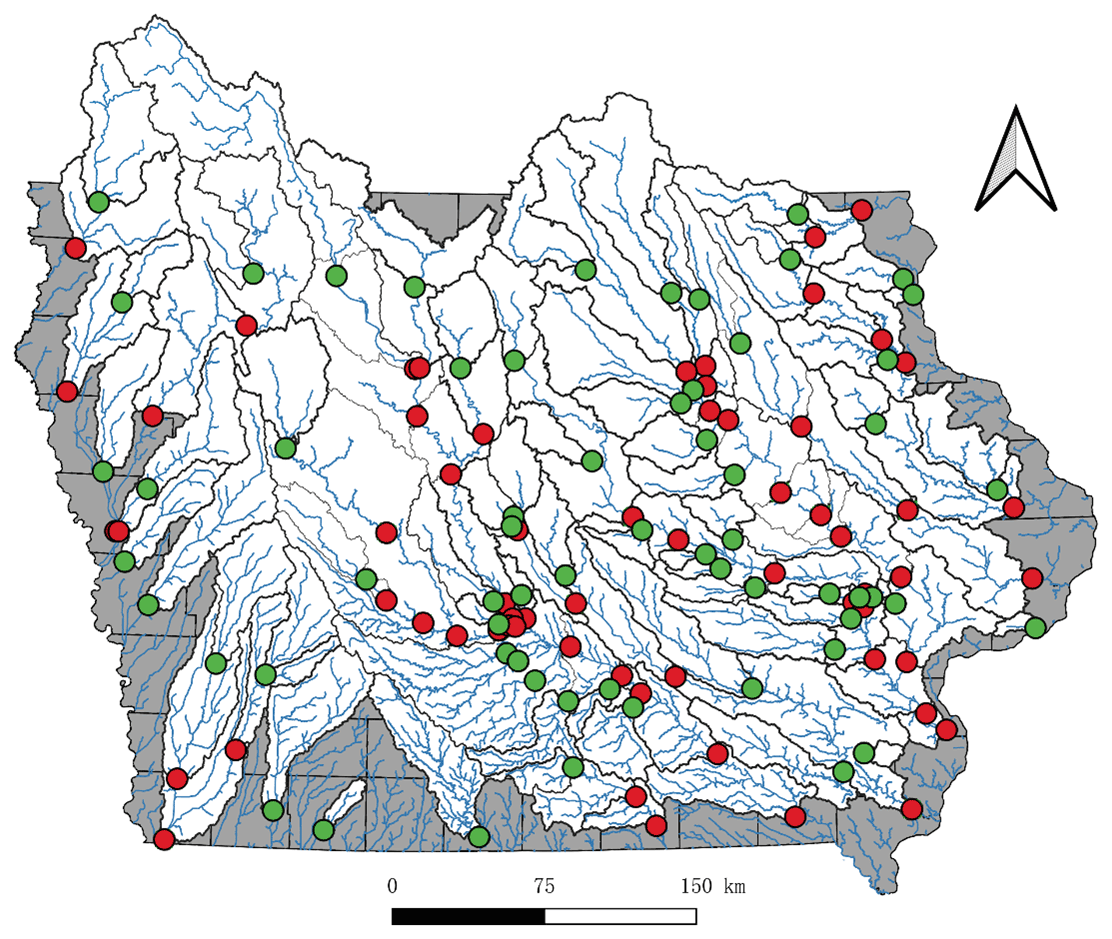
Figure 1The location of 125 USGS gauges in the State of Iowa for upstream sub-basins (green dot) and large downstream basins (red dot).
The United States Geological Survey (USGS) has over 100 streamflow gauges in the State of Iowa for monitoring the streamflow rate in different streams. The measurements from the USGS are typically recorded at 15–60 min intervals in Iowa. Due to site maintenance or shutdowns the coverage of the USGS streamflow gauges changes over the years. In this dataset, we selected all USGS gauges in the State of Iowa with available data from 1 October 2011 (the water year 2012) to 30 September 2018 (the water year 2018).
As shown in Fig. 1, red dots are located at the outlets of larger basins with multiple USGS gauges, which are divided into several smaller upstream sub-basins. The green dots are located at the outlets of the most upstream sub-basins. Thus, considering the connectivity of the streams, the relationship of these gauges in one watershed can be represented as a tree structure.
2.2 Dataset features
WaterBench includes detailed metadata and time-series features for each catchment. These datasets are available in .csv format for each catchment. The details of the datasets with data source, type, resolution and units are shown in Table 1. The statistics of the data, including the watershed size, concentration time (the longest streamflow path in the catchment), slope, and four soil types, are shown in Table 2 and Fig. 2. For each catchment, we provide static data (area, slope, travel time, etc.) as well as time series for streamflow, precipitation, and evapotranspiration (ET).
Table 1The details of datasets with data source, type, resolution and units.
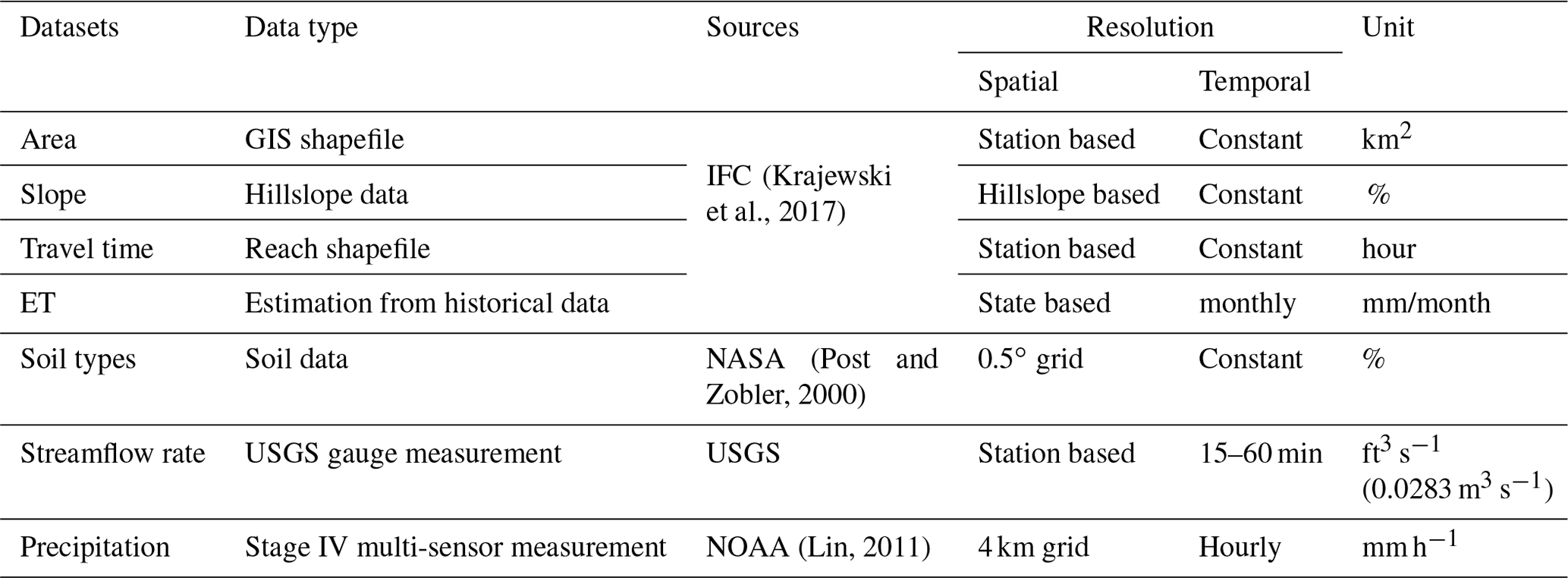
Table 2The minimum, maximum, mean, median, and standard deviation (SD) of the watershed area, concentration time, average slope, and percentage of soil types including loam, silt, sandy clay loam, and silty clay loam among 125 USGS gauges in the State of Iowa.
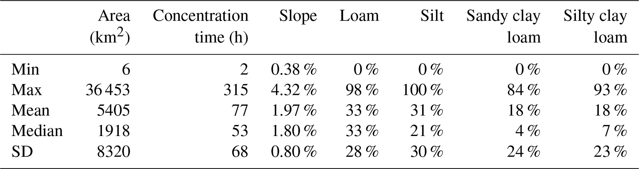
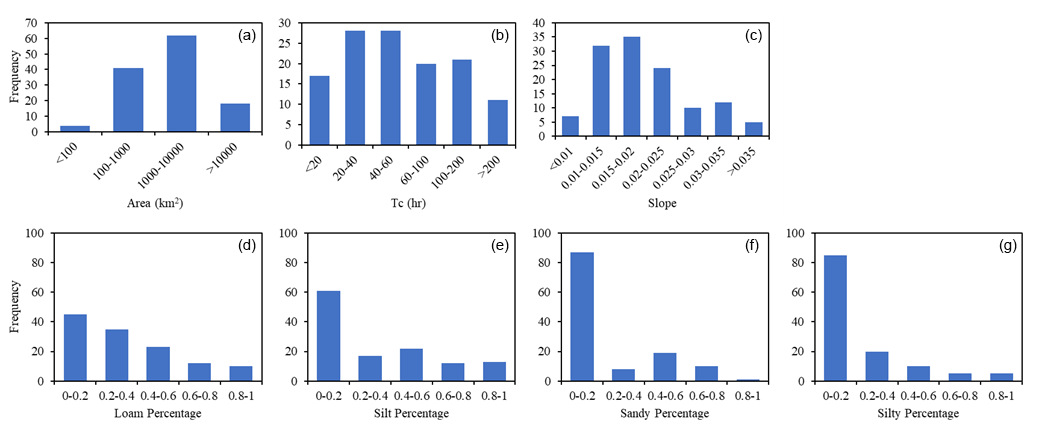
Figure 2Histograms of the catchment area (a), concentration time (b), average slope (c), and percentage of soil types including loam (d), silt (e), sandy clay loam (f), and silty clay loam (g) for 125 USGS gauges in the State of Iowa.
Table 3Summary statistics for precipitation and streamflow among 125 catchments from water year 2012–2018. Missing rate as a limitation.
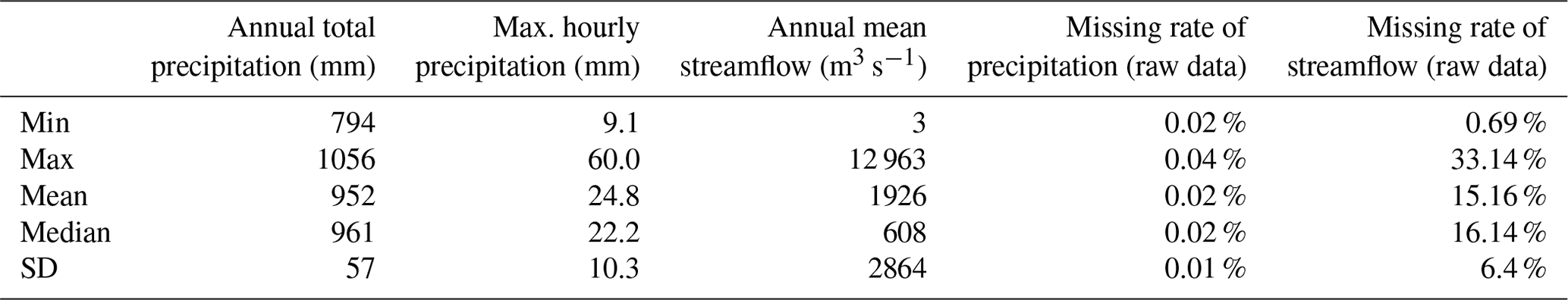
As shown in Table 3, all 125 catchments share similar precipitation ranges from 794 to 1056 mm, with a small standard deviation of 57 mm. Geologically, all the catchments are located in two HUC (hydrologic unit code) watersheds, the Upper Mississippi and Missouri rivers, and the study results may not be applicable to other regions in the USA. However, the modeling algorithms and the neural network architectures normally apply to a broad spectrum of problems, and they would be useful in other regions. WaterBench-Iowa is also subject to a relatively high missing data rate for streamflow as the reliable hourly dataset is limited by the USGS for some of the watersheds in Iowa. In the following sections, we will discuss the details of specific datasets and features.
2.2.1 Area
In the water cycle, precipitation is the main driving force of the streamflow. Based on the 90 m digital elevation model (DEM), only the precipitation in a certain area will contribute to a stream. Each measuring station has its corresponding area, which can be calculated from the watershed boundary shapefiles. Since the total precipitation amount is the product of precipitation intensity and area, in the same watersheds upstream sub-basins typically have lower streamflow rates than the larger basins. In WaterBench, the boundary shapefiles of each watershed are obtained from the Iowa Flood Information System (IFIS), a system operated by the Iowa Flood Center (IFC). Moreover, the area is calculated from the shapefiles in the unit of km2. Thus, the area contains one value per station, and it is available in the column of “area” in the “{station_id}_data.csv” files.
2.2.2 Time of concentration
The time of concentration provides the dimension of stream length for a watershed. In WaterBench, the time of concentration is defined as the longest length divided by the velocity, which is the time the water concentrates from the most distant point from the watershed outlet. The velocity used in this study is a constant value of 0.75 m s−1, which was found appropriate for Iowa catchments (Mandapaka et al., 2009; Mantilla et al., 2011), and has been successfully used in many hydrologic models (Fonley et al., 2016; Sloan et al., 2017). Thus, for a long and narrow watershed it may have a small watershed area but a large time of concentration. In WaterBench, the time of concentration is obtained from the IFIS with the unit of hours. Thus, the
time of concentration contains one value per station, and it is available in the column of “travel_time” in the “{station_id}_data.csv” files.
2.2.3 Slope
The slope is one of the topographic features that represents the slope gradient in percentage. A steep slope may cause a higher velocity and lower infiltration rate, which normally causes a larger streamflow rate during a precipitation event. The original file, hillslope map, is calculated by IFC (Sit et al., 2019), which splits the land of Iowa into over 600 000 hydrologic units using the algorithm developed by Mantilla and Gupta (2005). In WaterBench, the average slope is calculated from the mean value of the hillslopes in each catchment (Gericke and Du, 2012). Thus, the slope is a constant value per watershed, and it is available in the column of “slope” in the “{station_id}_data.csv” files.
2.2.4 Soil type
Soil type is one of the topographic features that represents the proportions of 12 different soil types on the land. Normally, the sandy soil has the largest infiltration rate, and the clay has the least infiltration rate. The original file, global soil types, is available from NASA (Post and Zobler, 2000). It is a 2-D map with a spatial resolution of 0.5∘. The soil type proportion is then calculated using the weighted average for each watershed. It should be noted that four dominant soil types, including the loam, silt, sandy clay loam, and silty clay loam, contribute to 99.91 % of the area in Iowa. Thus, only these four soil types are considered in the dataset. The percentage of each soil type is constant in the time-series dataset for each station in the columns of “loam”, “silt”, “sandy_clay_loam”, and “silty_clay_loam” in the “{station_id}_data.csv” files.
2.2.5 Streamflow rate
The streamflow rate is a variable measured by the USGS in the unit of cubic feet per second. The data was acquired from the USGS National Water Information System. There are nearly 200 real-time streamflow measuring stations in Iowa. After removing the stations established after 2011 or permanently closed before 2018, a total of 125 stations are selected, as shown in Fig. 1. For each station, streamflow data was aggregated to hourly values. The original data contains a few missing values due to station system failures or internet outages. For the stations located in the northern part of Iowa, the river may freeze and have no flow rate measurement over the winter, and all missing values were reported as −9999 by the USGS. In the dataset, each watershed has two columns, with the first column representing the timestamp from 1 October 2011 00:00 to 30 September 2018 23:00, and the second column representing the the streamflow values. Thus, the streamflow rate contains 61 368 values per station, and they are available in the column of “discharge” in the “{station_id}_data.csv” files.
2.2.6 Precipitation volume
Many station-based and satellite datasets have been measuring precipitation over the years. After comparisons, it is found that NOAA's Stage IV multi-sensor measurement is the most accurate (Seo et al., 2018) in the state of Iowa. The Stage IV multi-sensor provides the hourly precipitation amount with a 4 km-grid spatial resolution. The catchment level average precipitation is then calculated at each hour. Since there is no rainfall or snowfall most of the time, most precipitation values in the dataset are 0. In the dataset, we provide the hourly catchment-averaged precipitation data for each station from 1 October 2011 00:00 to 30 September 2018 23:00. Thus, the precipitation data contains 61 368 values per station, and they are available in the column of “precipitation” in the “{station_id}_data.csv” files.
2.2.7 Evapotranspiration (ET)
The ET represents the evaporation and plant transpiration from the land in the water cycle. It is one of the major losses of precipitated water. As no high-resolution real-time ET dataset is available, we used the monthly estimation from the historical measurement data in the past decades (Krajewski et al., 2017) as an empirical dataset. This is a monthly based dataset for the entire state of Iowa, and successfully captures the seasonal effects in the state of Iowa. In the dataset, we applied the ET value for each time stamp from 1 October 2011 00:00 to 30 September 2018 23:00. Thus, the ET data contains 61 368 values for all stations, and they are available in the column of “et” in the “{station_id}_data.csv” files.

Figure 3The median NSE and KGE among 125 watersheds in 125 different models at the prediction of the next 1–120 h.
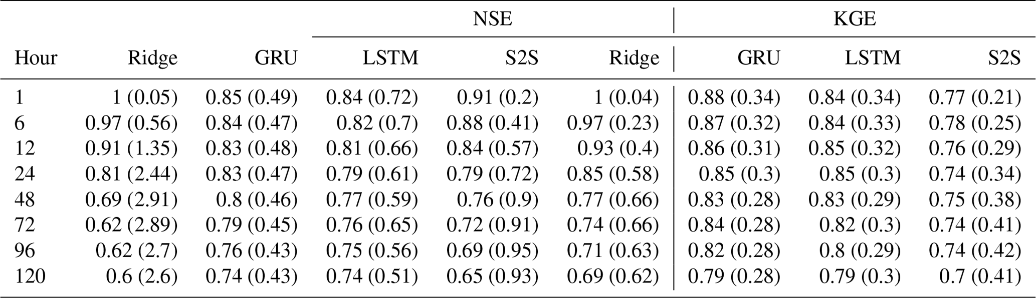
Table 4The median (standard deviation) NSE and KGE among 125 watersheds at the prediction hours 1, 6, 12, 24, 48, 72, 96, and 120 in 125 different models.
2.2.8 Watershed relationship
As many USGS measurement gauges are in the same watershed, many catchments in WaterBench-Iowa are not independent, and a relationship tree is given in the “catchment_relationship.csv”. The csv file represents a disconnected directed graph with each row representing an edge. Out of 125 catchments 63 have 1 or more upstream, as shown in the relationship, which are relatively large catchments. The remaining 62 catchments are specified as the very upstream catchments which have only 1 stream gauge. As these catchments have no overlapping areas, the catchments in our dataset form a disconnected graph. For the catchments that have overlapping areas, the watershed ID 646 has the largest connected subgraph with 27 upstream catchments. With upstream-downstream relationships, WaterBench-Iowa supports the cutting-edge studies such as graph neural networks.
In this section, we define a sample benchmark task of predicting the hourly streamflow for the next 5 d for future comparative studies. This task forecasts the future hourly floods at each hour as the National Water Model does. At each hour t, we predict the streamflow for the next 5 d from hour t+1–t+120 using all the data we can obtain at time t. In this task, we ignore the errors in the rainfall forecast, and use all the data including the topology data, the past 3 d precipitation and streamflow data, and the future 5 d precipitation data as input, to predict the streamflow for the next 120 h at the watershed outlet. Thus, we made 5 d predictions at each hour in the training and test datasets, and evaluated the results on different lead times from hour 1–hour 120. This task is a typical regression modeling of time series data. Therefore, we suggest the traditional ridge regression model and three deep learning models for modeling in this benchmark. Please refer to the recent studies for the detailed model structures such as LSTM (Kratzert et al., 2018), GRU (Gao et al., 2020) and S2S (Xiang and Demir, 2020).
We take two separate approaches to tackle this problem. The first approach involves a separate deep learning model for each of the available watersheds, while the second one involves building a single large regional model that carries out the same task for all available watersheds. For this specific task, we selected the last water year as the test set, and the rest as the training set. We further formatted the original dataset into a ready to use structure for each watershed with four files named as train_x, train_y, test_x, test_y. Thus, a total of 500 files for 125 watersheds are provided for this specific task. As general statistics, such as mean square error (MSE) and root mean square error (RMSE) are not dimensionless, the metrics for this study are Nash-Sutcliffe efficiency (NSE) and Kling-Gupta efficiency (KGE). They are both dimensionless statistics that are widely used in hydrological studies, and can be used to compare between watersheds. Both NSE and KGE range from negative infinity to 1, and the closer to 1 the better. The Eqs. (1) and (2) for NSE and KGE are shown below:
where Yi is the observation at the time i, is the model result at the time i, n is the total number of observations, r is the Pearson correlation coefficient, σ is the standard deviation, μ is the mean, σY is the standard deviation of all the observations, is the standard deviation of model forecasts, μY is the mean of all the observations and is the mean of all model forecasts.
Both NSE and KGE are dimensionless and in the range of (]. For both metrics, the closer to 1, better the model performs. We calculate the NSE and KGE based on the test year for each prediction hour. Since we predict the streamflow for the next 120 h at each hour, there will be 120 different NSE and KGE values for different hours at each watershed for the lead time from 1 to 120 h. It should be noted that since the watersheds here are not filtered, it is possible for some watersheds to be greatly affected by human activities, including mitigation, construction, irrigation, urban drainage, etc. activities in watersheds. Thus, a median value of all 125 watersheds is meaningful to report as a widely employed practice within other hydrology studies (Kratzert et al., 2018; Xiang et al., 2020). In addition, since the prediction accuracy typically decreases when the lead time increases, the median NSE and KGE of 125 stations at the 120 h forward predictions are the lowest. Thus, the 120 h ahead prediction scores are the most important metric that can represent the overall model performance on this task.
To provide baseline results over the sample benchmark task and two approaches defined in the previous section, we employed a linear regression model using ridge regression, and three deep learning models using LSTM, GRU, and S2S network architectures. For the first approach, we considered each watershed independently and trained one model for each watershed. Thus, the relationship between the watersheds is not used in this benchmark. The median NSE and KGE scores among 125 watersheds at each hour are shown in Fig. 3 and Table 4. As shown in the figure and the table, the ridge regression has a high accuracy in the first 24 h as the streamflow rates normally do not change too much in 1 d, and they are relatively easy to predict. The metrics for the medium-range show that the model using GRU has the best performance. The NSE and KGE histograms of GRU show that for most of the watersheds the GRU model performs well and the GRU model gives negative scores only in a limited number of watersheds. The standard deviations show relatively stable results in all prediction hours using deep learning models. However, the ridge model shows higher standard deviations and lower model performance than deep learning models over 48 h.
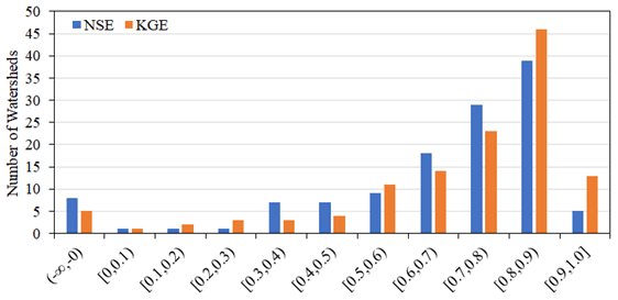
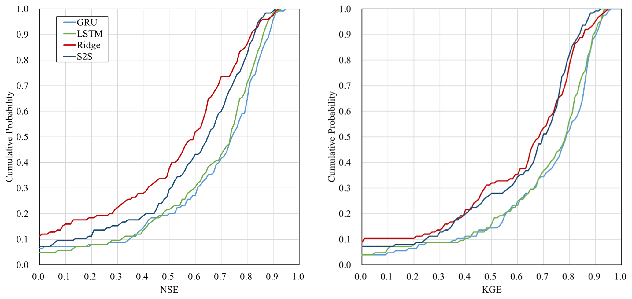
Figure 5 shows the cumulative distribution of the NSE and KGE among the 125 catchments at the lead time of 120 h in addition to the median value for all 125 catchments. The results suggest that there is a large standard deviation between catchments, and that negative NSE and KGE values occur in 10 % of the catchments. These catchments with negative NSE or KGE values are small (Fig. 7), so it is very challenging to predict the streamflow over 5 d.
As for the second approach, we attempted to develop single regional models for all 125 watersheds as they share similar physical attributes. As shown in Fig. 6, a single model of all 125 watersheds is possible with the physical features including area, slope, travel time, and soil types using the customized NSE loss function (Xiang et al., 2021). Among four models, similar to the first approach, the performance of ridge regression is hard to beat at first. Nevertheless, the deep learning model S2S starts to show a better performance starting the second day. Table 5 shows the detailed results of the regional model. Regional modeling using deep learning is more difficult as seen by the decline in model performance and greater standard deviations compared to the watershed modeling results in Table 4.
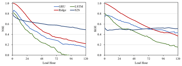
Figure 6The median NSE and KGE among 125 watersheds using one regional model at the prediction of the next 1–120 h.
Table 5The median (standard deviation) NSE and KGE among 125 watersheds at the prediction hour 1, 6, 12, 24, 48, 72, 96, and 120 using one regional model.
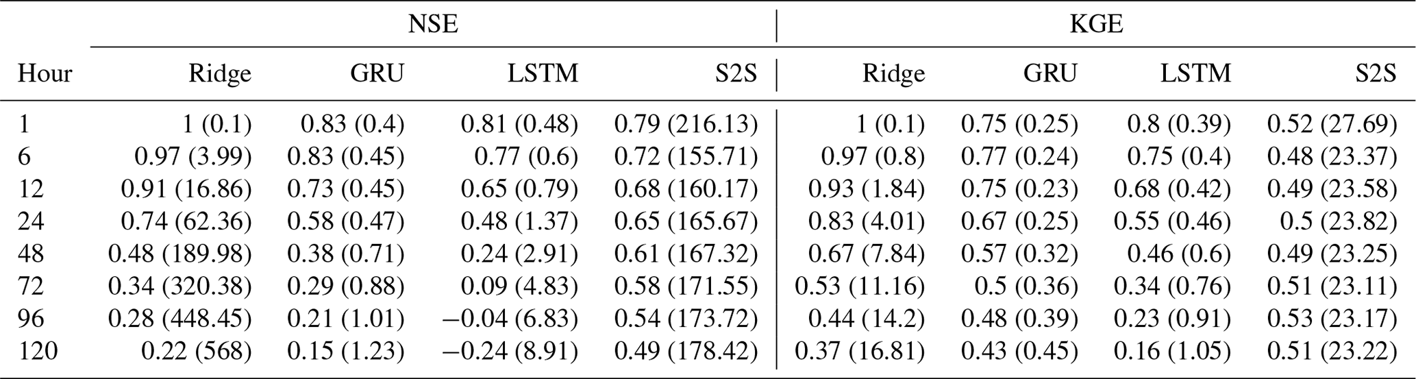
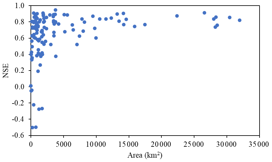
Figure 7The distribution of the 120 h ahead prediction using the best model in our benchmark (GRU for the single station).
As shown in the results, there are two major limitations. First, the model efficiency is low on the first day. It is shown in Fig. 3 and Table 4 that the deep learning models do not show a higher accuracy in the first several hours compared to the ridge model. Some hydrological studies have also shown that the basic persistence model (Streamflow t+n = Streamflow t) is hard to beat for short-range predictions when n is smaller than 12 h (Krajewski et al., 2020). Thus, it is hard to make both short-range and medium-range predictions accurately in one model. The second limitation is the scale effect, where the large basins have better model performance on the streamflow forecast and the small basins are hard to predict. The results show that as watersheds get larger the predictions become easier and better. This means the small watersheds, typically representing the middle and upper reaches, are harder to predict. Figure 7 shows the drainage area and 120 h ahead prediction performance in NSE for 125 watersheds. The scale effect observed in our benchmark indicates that the prediction in small watersheds is still a challenge.
Although a lot of metadata are provided in our dataset, as a benchmark our study does not consider complex pretreatment or models with domain knowledge in hydrology. Some recent studies have shown that the moving average for smoothing, the consideration of time lag, the consideration of watershed upstream-downstream connections, and other deep learning model architectures may be effective for a better prediction. However, these studies were based on their own datasets, and the results cannot be directly compared. We encourage researchers to conduct comparisons based on the WaterBench-Iowa.
The data and codes that support this study are openly available in Zenodo at https://doi.org/10.5281/zenodo.7087806 (Demir et al., 2022a). The dataset covers the 125 catchments in Iowa, USA with 7 different features, including precipitation, streamflow rate and ET with available data from 1 October 2011 (the water year 2012) to 30 September 2018 (the water year 2018). The original files of the dataset, metadata, and sample codes can be downloaded from archive files. The four different models, including ridge, LSTM, GRU, S2S, used in our paper are provided with ready-to-run Python Jupyter Notebooks as well (Demir et al., 2022b). The most recent code version can be found at https://github.com/uihilab/WaterBench (Demir et al., 2022b). Feedback by filing an issue on the repository would be welcomed.
In this study, by aggregating the datasets of watershed area, slope, soil types, streamflow, precipitation, and ET from NASA, NOAA, USGS, and IFC, we present a dataset, namely WaterBench-Iowa, that is prepared for an hourly streamflow forecast task. This dataset has a high temporal resolution with abundant geographic and relational information, which can be used for a variety of deep learning and machine learning application research. We defined a sample streamflow forecasting task for the next 120 h and provided example benchmark results on this task with a traditional linear and three customized deep learning models.
WaterBench-Iowa is not filtered and thus represents an actual streamflow forecast problem as much as possible. Although the data are limited to the Midwest, we believe that any studies on this dataset could provide insights into other streamflow forecasting and rainfall runoff modeling studies in other watersheds. With the open-source release of WaterBench-Iowa (https://github.com/uihilab/WaterBench, last access: 17 September 2022), this work provides a comparable benchmark, which to some extent makes up for the lack of a unified benchmark in hydrological and water resources research. We highly encourage other researchers to use the WaterBench-Iowa in their hydrological modeling research studies.
ID contributed to the conceptualization, project supervision and administration, funding acquisition, and review and editing. ZX contributed to the data curation, methodology, writing of method, results, and discussion. BD contributed to the software, validation, data analysis, dataset submission, and review and editing. MS contributed to conceptualization, investigation, supervision, writing of introduction and conclusion, and review and editing.
The contact author has declared that none of the authors has any competing interests.
Publisher's note: Copernicus Publications remains neutral with regard to jurisdictional claims in published maps and institutional affiliations.
This article is part of the special issue “Benchmark datasets and machine learning algorithms for Earth system science data (ESSD/GMD inter-journal SI)”. It is not associated with a conference.
The work reported in this study was made possible by the support of members of the Iowa Flood Center and the Department of Civil and Environmental Engineering at the University of Iowa. This research received no external funding. We sincerely appreciate all the valuable comments and suggestions from the editors and reviewers, which helped us improve the quality of the manuscript.
This paper was edited by Martin Schultz and reviewed by three anonymous referees.
Agliamzanov, R., Sit, M., and Demir, I.: Hydrology@ Home: a distributed volunteer computing framework for hydrological research and applications, J. Hydroinform., 22, 235–248, 2020.
Athira, V., Geetha, P., Vinayakumar, R., and Soman, K. P.: Deepairnet: Applying recurrent networks for air quality prediction, Proc. Comput. Sci., 132, 1394–1403, 2018.
Bai, Y., Bezak, N., Sapač, K., Klun, M., and Zhang, J.: Short-term streamflow forecasting using the feature-enhanced regression model, Water Resour. Manage., 33, 4783–4797, 2019.
Chung, J., Gulcehre, C., Cho, K., and Bengio, Y.: Empirical evaluation of gated recurrent neural networks on sequence modeling, arXiv [preprint], https://doi.org/10.48550/arXiv.1412.3555, 2014.
Cybenko, G.: Approximation by superpositions of a sigmoidal function, Math. Control Signal., 2, 303–314, 1989.
Deng, J., Dong, W., Socher, R., Li, L. J., Li, K., and Fei-Fei, L.: Imagenet: A large-scale hierarchical image database, in: 2009 IEEE conference on computer vision and pattern recognition, Miami, FL, USA, 20–25 June 2009 248–255, https://doi.org/10.1109/CVPR.2009.5206848, 2009.
Demir, I., Xiang, Z., Demiray, B. Z., and Sit, M.: WaterBench-Iowa: A Large-scale Benchmark Dataset for Data-Driven Streamflow Forecasting, Zenodo [data set and code], https://doi.org/10.5281/zenodo.7087806, 2022a.
Demir, I., Xiang, Z., Demiray, B. Z., and Sit, M.: WaterBench, GitHub [data set], https://www.github.com/uihilab/WaterBench, last access: 10 June 2022.
Demiray, B. Z., Sit, M., and Demir, I.: D-SRGAN: DEM > super-resolution with generative adversarial networks, SN Comput. Sci., 2, 1–11, 2021.
Du, S., Li, T., Yang, Y., and Horng, S. J.: Deep Air Quality Forecasting Using Hybrid Deep Learning Framework, IEEE T. Knowl. Data En., 33, 2412–2424, https://doi.org/10.1109/TKDE.2019.2954510, 2019.
Ebert-Uphoff, I., Thompson, D. R., Demir, I., Gel, Y. R., Karpatne, A., Guereque, M., Kumar, V., Cabral-Cano, E., and Smyth, P.: A vision for the development of benchmarks to bridge geoscience and data science, in: 17th International Workshop on Climate Informatics, Boulder, CO, USA, 20–22 September 2017, https://par.nsf.gov/servlets/purl/10143795 (last access: 10 June 2022), 2017.
Fonley, M., Mantilla, R., Small, S. J., and Curtu, R.: On the propagation of diel signals in river networks using analytic solutions of flow equations, Hydrol. Earth Syst. Sci., 20, 2899–2912, https://doi.org/10.5194/hess-20-2899-2016, 2016.
Franz, K. J., Hogue, T. S., and Sorooshian, S.: Operational snow modeling: Addressing the challenges of an energy balance model for National Weather Service forecasts, J. Hydrol., 360, 48–66, 2008.
Gao, S., Huang, Y., Zhang, S., Han, J., Wang, G., Zhang, M., and Lin, Q.: Short-term runoff prediction with GRU and LSTM networks without requiring time step optimization during sample generation, J. Hydrol., 589, 125188, https://doi.org/10.1016/j.jhydrol.2020.125188, 2020.
Gericke, O. J. and Du Plessis, J. A.: Catchment parameter analysis in flood hydrology using GIS applications, J. S. Afr. Inst. Civ. Eng., 54, 15–26, 2012.
Godfried, I., Mahajan, K., Wang, M., Li, K., and Tiwari, P.: FlowDB a large scale precipitation, river, and flash flood dataset, arXiv [preprint], https://doi.org/10.48550/arXiv.2012.11154, 2020.
Goodfellow, I., Bengio, Y., Courville, A. and Bengio, Y.: Deep learning, Vol. 1, Cambridge, MIT press, ISBN 978-0262035613, 2016.
Guo, T., Lin, T., and Lu, Y.: An interpretable LSTM neural network for autoregressive exogenous model, arXiv [preprint], https://doi.org/10.48550/arXiv.1804.05251, 2018.
Guo, Y., Zhang, L., Hu, Y., He, X., and Gao, J.: Ms-celeb-1m: A dataset and benchmark for large-scale face recognition, in: European conference on computer vision, ECCV2016 conference, Amsterdam, 8–16 October 2016, Springer, Cham, 87–102, https://doi.org/10.48550/arXiv.1607.08221, 2016.
Hochreiter, S. and Schmidhuber, J.: Long short-term memory, Neural Comput., 9, 1735–1780, 1997.
Hornik, K., Stinchcombe, M., and White, H.: Multilayer feedforward networks are universal approximators, Neural Networks, 2, 359–366, 1989.
Hu, C., Wu, Q., Li, H., Jian, S., Li, N., and Lou, Z.: Deep learning with a long short-term memory networks approach for rainfall-runoff simulation, Water, 10, 1543, https://doi.org/10.3390/w10111543, 2018.
Iowa Department of Natural Resources: Chapter 1 Iowa's Water Resources, http://www.iowadnr.gov/portals/idnr/uploads/water/watershed/files/nonpoint plan/nps04.pdf, last access: 10 June 2022.
Krajewski, W. F., Ceynar, D., Demir, I., Goska, R., Kruger, A., Langel, C., Mantilla, R., Niemeier, J., Quintero, F., Seo, B., Small, S., Weber, L., and Young, N.: Real-time flood forecasting and information system for the state of Iowa, B. Am. Meteorol. Soc., 98, 539–554, https://doi.org/10.1175/BAMS-D-15-00243.1, 2017.
Krajewski, W. F., Ghimire, G. R., and Quintero, F.: Streamflow Forecasting without Models, J. Hydrometeorol., 21, 1689–1704, 2020.
Kratzert, F., Klotz, D., Brenner, C., Schulz, K., and Herrnegger, M.: Rainfall–runoff modelling using Long Short-Term Memory (LSTM) networks, Hydrol. Earth Syst. Sci., 22, 6005–6022, https://doi.org/10.5194/hess-22-6005-2018, 2018.
Kratzert, F., Klotz, D., Herrnegger, M., Sampson, A. K., Hochreiter, S., and Nearing, G. S.: Toward improved predictions in ungauged basins: Exploiting the power of machine learning, Water Resour. Res., 55, 11344–11354, 2019.
LeCun, Y., Bengio, Y., and Hinton, G.: Deep learning, Nature, 521, 436–444, 2015.
Leshno, M., Lin, V. Y., Pinkus, A., and Schocken, S.: Multilayer feedforward networks with a nonpolynomial activation function can approximate any function, Neural Networks, 6, 861–867, 1993.
Li, Y., Zhu, Z., Kong, D., Han, H., and Zhao, Y.: EA-LSTM: Evolutionary attention-based LSTM for time series prediction, Knowl.-Based Syst., 181, 104785, https://doi.org/10.1016/j.knosys.2019.05.028, 2019.
Lin, Y.: GCIP/EOP Surface: Precipitation NCEP/EMC 4KM Gridded Data (GRIB) Stage IV Data, version 1.0, UCAR/NCAR Earth Observing Laboratory [data set], https://data.eol.ucar.edu/dataset/21.093 (last access: 10 June 2022), 2011.
Liu, W., Guo, G., Chen, F., and Chen, Y.: Meteorological pattern analysis assisted daily PM2.5 grades prediction using SVM optimized by PSO algorithm, Atmos. Pollut. Res., 10, 1482–1491, 2019.
Mandapaka, P. V., Krajewski, W. F., Mantilla, R., and Gupta, V. K.: Dissecting the effect of rainfall variability on the statistical structure of peak flows, Adv. Water Resour., 32, 1508–1525, 2009.
Mantilla, R. and Gupta, V. K.: A GIS numerical framework to study the process basis of scaling statistics in river networks, IEEE Geosci. Remote S., 2, 404–408, 2005.
Mantilla, R., Gupta, V. K., and Troutman, B. M.: Scaling of peak flows with constant flow velocity in random self-similar networks, Nonlin. Processes Geophys., 18, 489–502, https://doi.org/10.5194/npg-18-489-2011, 2011.
Maskey, M., Alemohammad, H., Murphy, K. J., and Ramachandran, R.: Advancing AI for Earth science: A data systems perspective, EOS, 101, https://doi.org/10.1029/2020EO151245, 2020.
McEnery, J., Ingram, J., Duan, Q., Adams, T., and Anderson, L.: NOAA's advanced hydrologic prediction service: building pathways for better science in water forecasting, B. Am. Meteorol. Soc., 86, 375–386, 2005.
Newman, A., Sampson, K., Clark, M., Bock, A., Viger, R., and Blodgett, D.: A large sample watershed-scale hydrometeorological dataset for the contiguous USA, UCAR/NCAR, Boulder, CO, https://doi.org/10.5065/D6MW2F4D, 2014.
Post, W. M. and Zobler, L.: Global Soil Types, 0.5-Degree Grid (Modified Zobler), ORNL DAAC [data set], Oak Ridge, Tennessee, USA, https://doi.org/10.3334/ORNLDAAC/540, 2000.
Reichstein, M., Camps-Valls, G., Stevens, B., Jung, M., Denzler, J., and Carvalhais, N.: Deep learning and process understanding for data-driven Earth system science, Nature, 566, 195–204, 2019.
Sagheer, A. and Kotb, M.: Unsupervised pre-training of a Deep LStM-based Stacked Autoencoder for Multivariate time Series forecasting problems, Sci. Rep., 9, 1–16, 2019.
Seeger, M., Salinas, D., and Flunkert, V.: Bayesian intermittent demand forecasting for large inventories, in: Proceedings of the 30th International Conference on Neural Information Processing Systems, 4653–4661, ISBN 9781510838819, 2016.
Seo, B. C., Krajewski, W. F., Quintero, F., ElSaadani, M., Goska, R., Cunha, L. K., and Petersen, W. A.: Comprehensive evaluation of the IFloodS radar rainfall products for hydrologic applications, J. Hydrometeorol., 19, 1793–1813, 2018.
Seo, B. C., Keem, M., Hammond, R., Demir, I., and Krajewski, W. F.: A pilot infrastructure for searching rainfall metadata and generating rainfall product using the big data of NEXRAD, Environ. Modell. Softw., 117, 69–75, 2019.
Sit, M. and Demir, I.: Decentralized flood forecasting using deep neural networks, arXiv [preprint], https://doi.org/10.48550/arXiv.1902.02308, 2019.
Sit, M., Sermet, Y., and Demir, I.: Optimized watershed delineation library for server-side and client-side web applications, Open Geospatial Data, Software and Standards, 4, 1–10, 2019.
Sit, M., Demiray, B. Z., Xiang, Z., Ewing, G. J., Sermet, Y., and Demir, I.: A comprehensive review of deep learning applications in hydrology and water resources, Water Sci. Technol., 82, 2635–2670, 2020.
Sit, M., Demiray, B., and Demir, I.: Short-term hourly streamflow prediction with graph convolutional gru networks, arXiv [preprint], https://doi.org/10.48550/arXiv.2107.07039 2021a.
Sit, M., Seo, B. C., and Demir, I.: Iowarain: A statewide rain event dataset based on weather radars and quantitative precipitation estimation, arXiv [preprint], https://doi.org/10.48550/arXiv.2107.03432 2021b.
Sloan, B. P., Mantilla, R., Fonley, M., and Basu, N. B.: Hydrologic impacts of subsurface drainage from the field to watershed scale, Hydrol. Process., 31, 3017–3028, 2017.
Su, S., Delbracio, M., Wang, J., Sapiro, G., Heidrich, W., and Wang, O.: Deep video deblurring for hand-held cameras, in: Proceedings of the IEEE Conference on Computer Vision and Pattern Recognition, 1279–1288, 2017.
Tao, Q., Liu, F., Li, Y., and Sidorov, D.: Air pollution forecasting using a deep learning model based on 1D convnets and bidirectional GRU, IEEE Access, 7, 76690–76698, 2019.
Vaswani, A., Shazeer, N., Parmar, N., Uszkoreit, J., Jones, L., Gomez, A. N., Kaiser, Ł., and Polosukhin, I.: Attention is all you need, arXiv [preprint], https://doi.org/10.48550/arXiv.1706.03762, 2017.
Wilkinson, M. D., Dumontier, M., Aalbersberg, I. J., Appleton, G., Axton, M., Baak, A., and Mons, B.: The FAIR Guiding Principles for scientific data management and stewardship, Sci. Data, 3, 1–9, 2016.
Xiang, Z. and Demir, I.: Distributed long-term hourly streamflow predictions using deep learning – A case study for State of Iowa, Environ. Modell. Softw., 131, 104761, https://doi.org/10.1016/j.envsoft.2020.104761, 2020.
Xiang, Z., Yan, J., and Demir, I.: A rainfall-runoff model with LSTM-based sequence-to-sequence learning, Water Resour. Res., 56, e2019WR025326, https://doi.org/10.1029/2019WR025326, 2020.
Xiang, Z., Demir, I., Mantilla, R., and Krajewski, W. F.: A Regional Semi-Distributed Streamflow Model Using Deep Learning, EarthArXiv, https://doi.org/10.31223/X5GW3V, 2021.
Xu, H., Windsor, M., Muste, M., and Demir, I.: A web-based decision support system for collaborative mitigation of multiple water-related hazards using serious gaming, J. Environ. Manage., 255, 109887, https://doi.org/10.1016/j.jenvman.2019.109887, 2020.
Xue, T., Chen, B., Wu, J., Wei, D., and Freeman, W. T.: Video enhancement with task-oriented flow, Int. J. Comput. Vis., 127, 1106–1125, 2019.
Yildirim, E., and Demir, I.: An Integrated Flood Risk Assessment and Mitigation Framework: A Case Study for Middle Cedar River Basin, Iowa, US, Int. J. Disast. Risk Re., 56, 102113, https://doi.org/10.1016/j.ijdrr.2021.102113, 2021.
Yu, H. F., Rao, N., and Dhillon, I. S.: Temporal Regularized Matrix Factorization for High-dimensional Time Series Prediction, in: Proceedings of Advances in Neural Information Processing Systems, 29, 847–855, ISBN 9781510838819, 2016.
Zhang, J., Zhu, Y., Zhang, X., Ye, M., and Yang, J.: Developing a Long Short-Term Memory (LST) based model for predicting water table depth in agricultural areas, J. Hydrol., 561, 918–929, https://doi.org/10.1016/j.jhydrol.2018.04.065, 2018.
Zhu, S., Lian, X., Wei, L., Che, J., Shen, X., Yang, L., and Li, J.: PM2.5 forecasting using SVR with PSOGSA algorithm based on CEEMD, GRNN and GCA considering meteorological factors, Atmos. Environ., 183, 20–32, 2018.