OpenMRG: Open data from Microwave links, Radar, and Gauges for rainfall quantification in Gothenburg, Sweden

Accurate rainfall monitoring is critical for sustainable societies and yet challenging in many ways. Opportunistic monitoring using commercial microwave links (CMLs) in telecommunication networks is emerging as a powerful complement to conventional gauges and weather radar. However, CML data are often inaccessible or incomplete, which limits research and application. Here, we aim to reduce this barrier by openly sharing data at 10 s resolution with true coordinates from a pilot study involving 364 bi-directional CMLs in Gothenburg, Sweden. To enable further comparative analyses, we also share high-resolution data from 11 precipitation gauges and the Swedish operational weather radar composite in the area. This article presents an overview of the data, including the collection approach, descriptive statistics, and a case study of a high-intensity event. The results show that the data collection was very successful, providing near-complete time series for the CMLs (99.99 %), gauges (100 %), and radar (99.6 %) in the study period (June–August 2015). The bandwidth consumed during CML data collection was small, and hence, the telecommunication traffic was not significantly affected by the collection. The gauge records indicate that total rainfall was approximately 260 mm in the study period, with rainfall occurring in 6 % of each 15 min interval. One of the most intense events was observed on 28 July 2015, during which the Torslanda gauge recorded a peak of 1.1 mm min⁻¹. The variability in the CML data generally followed the gauge dynamics very well. Here we illustrate this for 28 July, where a nearby CML recorded a drop in received signal level of about 27 dB at the time of the peak. The radar data showed a good distribution of reflectivities for mostly stratiform precipitation but also contained some values above 40 dBZ, which is commonly seen as an approximate threshold for convective precipitation. Clutter was also found and was mostly prevalent around low reflectivities of −15 dBZ. The data are accessible at https://doi.org/10.5281/zenodo.7107689 (Andersson et al., 2022). We believe this Open sharing of high-resolution data from Microwave links, Radar, and Gauges (OpenMRG) will facilitate research on microwave-based environmental monitoring using CMLs and support the development of multi-sensor merging algorithms.

1 Introduction

Monitoring rainfall is of critical importance to society in many different ways, e.g. for the design of infrastructure, for post-analysis of rainfall-induced problems and disasters, for hydrological modelling and flood forecasting, and for assessing climate variability and change. Heavy precipitation is already intensifying as a function of global warming, e.g. in northern Europe (Masson-Delmotte et al., 2021), and this intensification is expected to continue (e.g. Olsson et al., 2017). Monitoring is, however, highly challenging due to the extreme spatiotemporal variability in rainfall. Rain gauges are still considered the most reliable, even though these are also known to give erroneous measurements (Habib et al., 2001; Sieck et al., 2007). Additionally, gauge networks are typically small or sparse (or both) and will therefore inevitably miss spatial information outside the network and between the gauges.

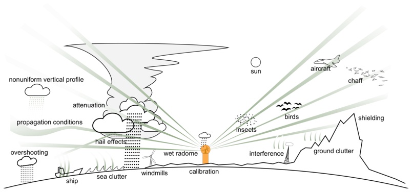
Figure 1 Example of error sources effecting weather radar measurements. Figure provided by Markus Peura, Finnish Meteorological Institute (FMI), and used with permission.

In the last few decades, weather radar has emerged as a key complementary rainfall observation technique. Radar pulses are transmitted in all directions, and rainfall intensity may be estimated from their echoes. The key advantage is full spatial coverage in a circle around the radar. However, rainfall intensity is uncertain due to a range of error sources, e.g. clutter, attenuation, and anomalous propagation (Battan, 1973; Zawadzki, 1984; van de Beek et al., 2016). An illustration of error sources can be found in Fig. 1. There is a need to also explore other techniques for rainfall monitoring, especially in developing countries where gauge networks are often insufficient and expensive radar systems are scarce.

The concept of using commercial microwave links (CMLs) in operational telecommunication networks for the monitoring of rainfall and other environmental variables has been explored for about 15 years (Messer et al., 2006; Leijnse et al., 2007). The methodology to measure rainfall using microwave links exploits the power attenuation of an electromagnetic wave when it propagates through water drops. The physical foundations have been studied theoretically and empirically since the 1970s, and it is today well established that radio signals above 10 GHz are sensitive to rain, and the resulting power attenuation increases as frequency increases (ITU, 2005; Atlas and Ulbrich, 1977; Olsen et al., 1978). Even if the conversion from attenuation to spatiotemporal rainfall fields is not trivial and requires a number of processing steps, estimating rainfall based on microwave links is a highly promising complement to gauges and radars, particularly when considering the very high resolutions in space and time attainable through the existing infrastructure, and their widespread operational use globally (Messer et al., 2006; Overeem et al., 2016; Fencl et al., 2015; Graf et al., 2021; Doumounia et al., 2014; Nebuloni et al., 2022; van de Beek et al., 2020; Ericsson, 2018).

A major constraint for research on CMLs in operational networks concerns data access (Chwala and Kunstmann, 2019). CML data are typically only available to mobile network operators and the research groups they collaborate with. Given the potential of CMLs to act as opportunistic rainfall sensors, the data are, however, of general scientific interest, which is underlined by the recently established OPENSENSE network (https://www.cost.eu/actions/CA20136/, last access: 29 November 2022). A few research groups have been able to share some CML data openly. Špačková et al. (2021) provided a 1-year data set for one dual-polarized microwave link sampled every ∼ 4 s, along with disdrometers, rain gauges, and conventional weather variables in Switzerland. Fencl et al. (2020, 2021) shared data from six E-band CMLs sampled every ∼ 10 s, along with conventional gauge measurements of rainfall, temperature, and humidity during 4 and 7 months, respectively, in the Czech Republic. Overeem (2019) presented aggregated signal strength statistics at 15 min and ± 1 dB resolution from ∼ 2500 CMLs (derived from standard operational network management systems) and radar data covering the Netherlands. Habi (2020) shared data from two CMLs in Israel, and van Leth et al. (2018) provided data for three research links in the Netherlands.

In order to significantly extend the open CML database available for research and benchmarking, the main objective of this paper is to make available a set of CML data collected during a pilot project in Sweden. It consists of transmitted and received signal levels from an operational network of 364 CMLs around Gothenburg during the summer months of 2015. The data are provided at a high temporal resolution (10 s) and with true coordinates. To enable comparative analyses and algorithm development, we also include data from a set of precipitation gauges, one meteorological station, and weather radar. Together, this makes the Open data from Microwave links, Radar, and Gauges (OpenMRG) unique, providing data for many operational CMLs at high temporal resolution and with precise coordinates, along with gauge and radar data.

In Sect. 2, the origin and collection approach of the included data sets are described. In Sect. 3, we proceed to describe the methods applied to present and analyse the data. Subsequently, Sect. 4 presents the results of the data collection and the characteristics of the data. After some discussion about known challenges and potential applications in Sect. 5, information on data availability is given in Sect. 6 and some concluding remarks in Sect. 7. We hope this effort will encourage cross-disciplinary research in different related fields, e.g. environmental monitoring, sensor networks, big data analytics, machine learning, and hydrometeorological forecasting.

2 Study area and data collection

The data sets presented here stem from a pilot project involving the Swedish Meteorological and Hydrological Institute (SMHI), the telecom company Ericsson, and the mobile network operator Hi3G Sweden, which was initially reported at the 15th International Conference on Environmental Science and Technology (Bao et al., 2017; Andersson et al., 2017). The data cover the city of Gothenburg, Sweden, and its surroundings (Fig. 2) for the period 1 June to 31 August 2015 (JJA 2015). The OpenMRG data set consists of data from three types of rainfall sensors (CMLs, rainfall gauges, and weather radar) and standard meteorological parameters (temperature, humidity, pressure, and wind).

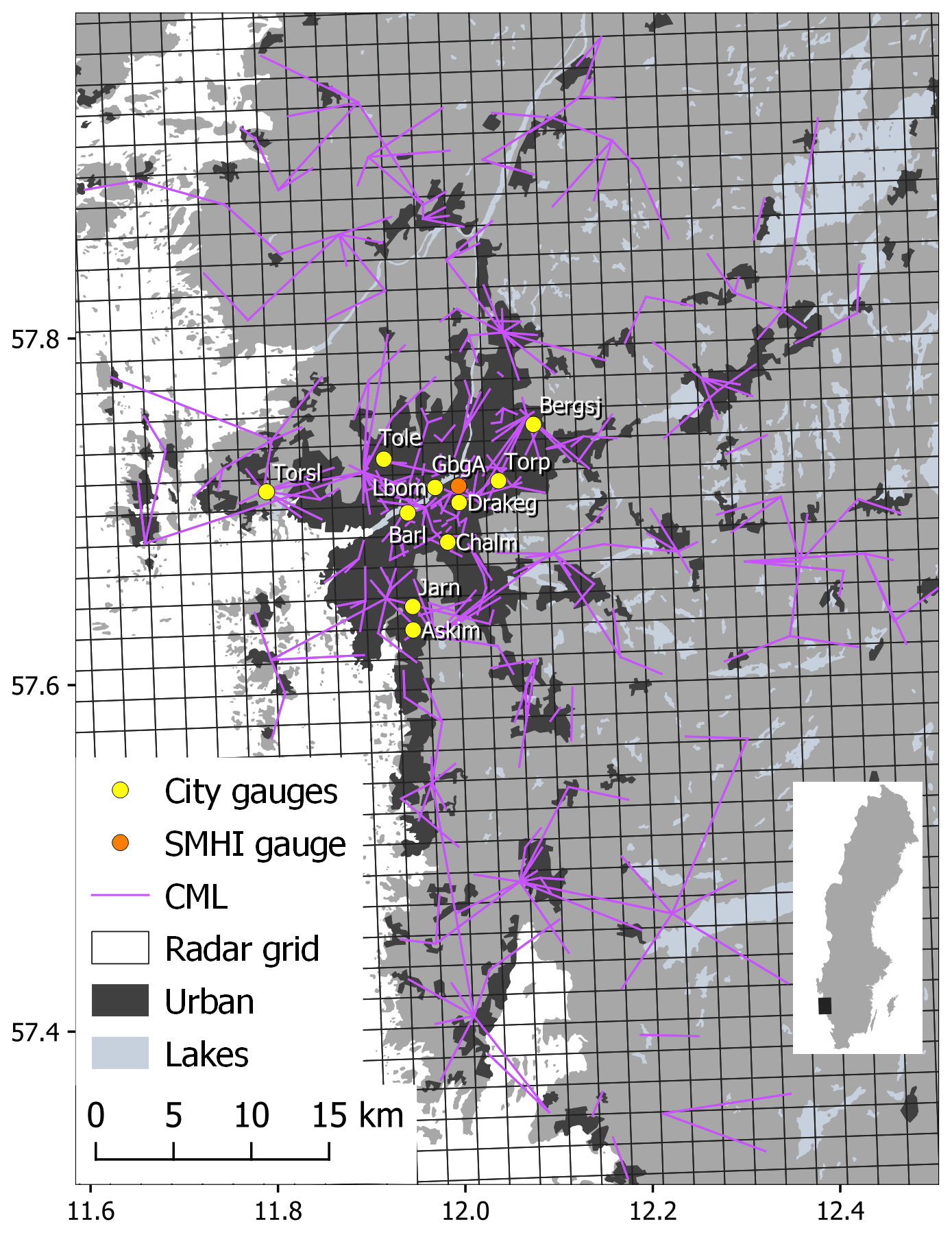
Figure 2 Map of Gothenburg, Sweden, showing an overview of the data sets presented in this study. The inset map of Sweden shows the study area as a black square.

2.1 Microwave links

For clarity, a set of terms are used to describe the CML data in this article. A “node” is the location at which the antenna of one or more microwave radios is installed (typically a telecommunication mast). A “sub-link” is a specific connection between two nodes, from a transmitting antenna (providing transmitted signal level data, TSL) to a receiving antenna (providing received signal level data, RSL). A “link” consists of all sub-links operating between two antennas. A link usually consists of two paired sub-links (one in each direction) but can consist of more, depending on the design. Finally, a “hop” consists of all links operating between two specific nodes (e.g. one link operating at 18 GHz and another at 32 GHz). Figure 3 illustrates these terms. Here we use the term “signal level”, which is sometimes alternatively called “signal strength” or “signal power”. For consistency, we also use “TSL” and “RSL” instead of “TX” and “RX”, respectively, which are also sometimes used. Equally, what we here refer to as a “node” is sometimes called a “site”.

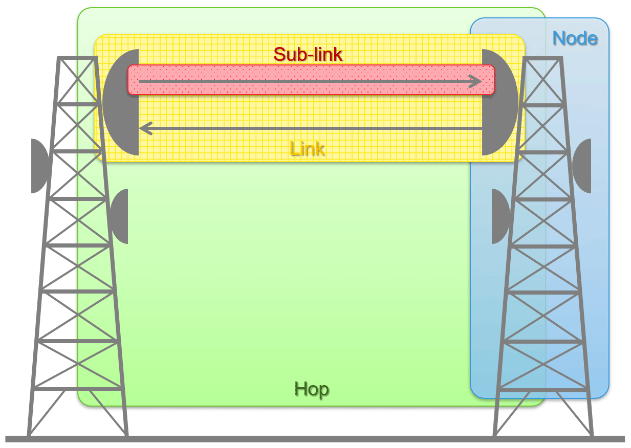
Figure 3 Conceptual representation of a “node”, “sub-link”, “link”, and “hop”, respectively, as used to describe CML network features in this study. One “link” is here equivalent to one “CML”.

Table 1 General characteristics of the microwave link network.

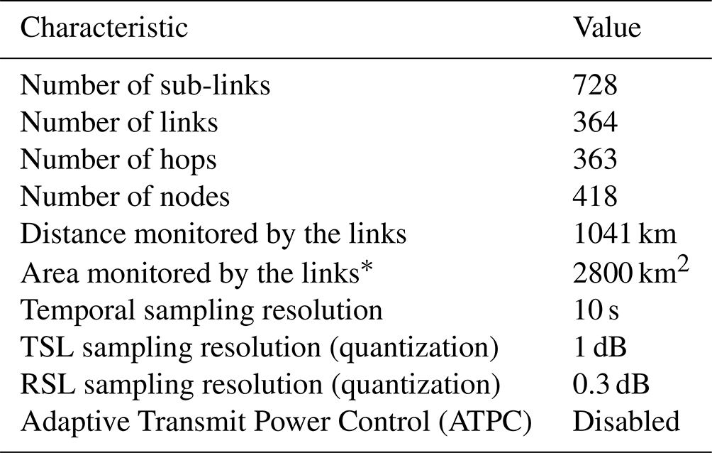
^∗ Approximated by a convex hull around the CML network.

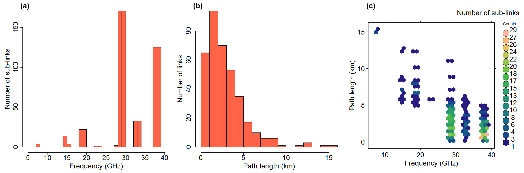
Figure 4 CML network characteristics. (a) Distribution of carrier frequencies. (b) Distribution of path lengths. (c) Relationship between path length, frequency, and number of sub-links.

The CML data originate from a subset of the operational microwave mobile backhaul network of the telecom operator Hi3G, specifically 728 sub-links operating using Ericsson MINI-LINK radios (Table 1). More background is also provided by Ericsson (2022) and Morais (2021; see particularly chapter 7 on the “Transceiver Architecture, Link Capacity, and Example Specification”). For each sub-link, a set of metadata were compiled (ID, coordinates, frequency, polarization, and antenna diameter) which were extracted from the operator's network planning database. The network consists primarily of vertically polarized sub-links, operating at carrier frequencies between 7 and 38 GHz, with a majority above 25 GHz (Fig. 4a). Paired sub-links typically operate at similar frequencies (differing up to 1.5 GHz in the forward and reverse direction), which is the reason for the pairs in the histogram in Fig. 4a. The path lengths of the links vary between 100 m and 15 km, with a median of approximately 2 km (Fig. 4b). Higher-frequency sub-links are typically installed at shorter distances (Fig. 4c) to ensure robust operations despite increasing rainfall attenuation. The antenna diameters vary between 20 cm and 1.2 m, with a corresponding antenna gain ranging between 31 and 47 dBi. In general, the antenna gain increases as antenna size and carrier frequency increase. The antennas were installed at approximately 30 m above ground on average, and altitude variations in the area are negligible.

Figure 5 Map of the microwave link network in Gothenburg, Sweden, showing the (a) carrier frequency and (b) sub-link density.

The CML network in Gothenburg has a star-shaped topology, i.e. with several links originating from the same node (Fig. 5). Relatively short and higher-frequency links are more prevalent in the city centre, while longer, low-frequency links are more common in the peripheral areas (Fig. 5a). The network density is highest in the heart of Gothenburg, with at least 10 sub-links per square kilometre (Fig. 5b). This can be advantageous from several perspectives, including accuracy (using multiple crossing links of varying frequencies to estimate rainfall), resolution (providing spatial information at sub-kilometre resolution), and operational robustness (rainfall can be estimated even if some links are non-operational). The network density rapidly declines as the distance from urban areas increases, with large areas being covered only by one link.

The collection of CML data from the Hi3G network was carried out by Ericsson. The CML monitoring system consisted of a data collection service (DC) and a data mediation service (DM). The DC was located inside Hi3G's network and utilized the Simple Network Management Protocol (SNMP) to sample and store transmitted and received signal levels every 10 s from a predefined set of nodes in the network. A software package, using standard SNMP, was developed and applied to obtain this temporal resolution, but no firmware changes at the nodes were required. The sampling was carried out toward 150 nodes in parallel, and then sequentially until all nodes had been sampled. This procedure was initiated every 10 s, and continued during a 7 s sampling window, which means that the exact sampling time varied slightly between nodes (and hence also between TSL and RSL values for a single sub-link). However, our analysis of the sampling indicates that all nodes were likely sampled within ± 1 s in this network. The subsequent sampling of nodes followed the same sequence to stay as close as possible to the target 10 s sampling interval.

Every minute, the collected data were transferred to the DM located at Ericsson. The DM compiled the data for further processing, e.g. mapping transmitting and receiving nodes, synchronizing time stamps (i.e. to be the start of each sampling window for all nodes), and assigning suitable IDs. In this process, values representing specific error codes or values that were outside of expected ranges were filtered out; specifically, TSL ≤ −99, TSL = 255, RSL ≤ −99.9, and RSL > −20 were set to missing. Such values appear due to radio timeout issues, when no signal was received, or due to other hardware impairments. Ericsson forwarded the data to SMHI in zipped TXT format. To obtain a regular time series, SMHI rounded the time steps to the nearest 10 s. This affected 67 % of the time steps, for which the sampling window originally started on second 59, 09, 19, 29, 39, and 49 instead of 00, 10, 20, 30, 40, and 50, respectively. Finally, SMHI calculated link lengths (great circle distance) and structured the data into a netCDF file to facilitate further processing. The collection system was designed in a flexible manner to enable a varying temporal sampling resolution and link network and to enable potential extensions in the future.

The OpenMRG data set consists of TSL and RSL time series. These can be converted to rainfall intensity using different methods, each with their own assumptions, advantages, and disadvantages. However, most methods are based on the following general approach building on, for example, Olsen et al. (1978) and ITU (2005). First, the time series are scrutinized to filter out any erroneous or dubious data. The signal attenuation is subsequently derived by calculating the difference between TSL and RSL. Each time step is classified as wet or dry, e.g. using average conditions, signal variability, or pattern recognition. A baseline attenuation is defined for the wet time steps that is typically based on the attenuation levels during adjacent dry time steps. Subsequently, the specific attenuation (i.e. normalized by link length) exceeding the baseline during wet time steps is derived (k; dB km⁻¹). Rainfall intensity (R; mm h⁻¹) is then calculated from k using an inverted power law equation, as follows:

$$\begin{array}{}\text{(1)}& k=c{R}^d,\end{array}$$

where parameters c and d depend on the frequency and polarization, for which ITU (2005) provide standard values. Normally, one or more steps are also introduced to compensate for non-rain signal fluctuations, e.g. accounting for wet-antenna attenuation. The resulting rainfall intensity time series (one for each sub-link) can finally be combined using spatial interpolation methods to produce complete spatiotemporal fields. The pycomlink software package by Chwala et al. (2022) provides a useful implementation of this general approach.

2.2 Gauges

Two sets of observations from rainfall gauges are included in the OpenMRG data set. The first set is a time series of 15 min observations from station “GbgA” in the national network of automatic weather stations operated by SMHI (these data are hereafter denoted “SMHI gauge”). The gauge, located in central Gothenburg (Fig. 2), is of a weighing type (by Geonor), with a 0.1 mm resolution which uses a precision vibrating wire transducer to weigh the precipitation collected. A thin layer of oil is added to impede any evaporation, which can essentially eliminate evaporation even during long periods without maintenance. The gauge is equipped with a wind screen in the form of metal or plastic plates that minimize precipitation losses, but still some wind-induced undercatch is likely to occur, e.g. caused by wind gusts and updrafts associated with intense convective activity. Several other meteorological parameters are collected at the GbgA station, and we here include hourly observations of air temperature, relative humidity, air pressure, wind speed (average and gust), and wind direction. The observations have been quality controlled in the database system of SMHI.

The second set of rainfall observations comes from a gauge network operated by Gothenburg city (these data are hereafter denoted “City network”). The network comprises 10 gauges well distributed over the entire city (Fig. 2). Seven of these gauges are Geonor weighing gauges, i.e. the same type as the SMHI gauge. The other three are of a tipping-bucket type with a 0.2 mm resolution. The altitude of the City network gauges is unknown, but typically, such sensors are placed approximately 1.5 m above ground. Originally, the City network data were stored and provided with entries only for time steps with some recorded rainfall (i.e. without zeros or data quality flags). In the OpenMRG data set, we transformed all observations from the City network to complete 1 min time series by accumulating the recorded volumes from second 01 in the preceding minute until second 00 of the minute given in the timestamp. Some known errors in the data were also removed, but the data did not go through the same rigorous quality control procedure as the SMHI gauge data.

Table 2 Metadata of the radar data set with a 5 min temporal resolution. Here the x and y scale represents the number of grid points in each direction and x and y size the spatial resolution of each grid cell. The upper left (UL) and lower right (LR) latitude (lat) and longitude (lon) coordinates are provided by the final four parameters. The projection is given as a “proj” string (https://proj.org/, last access: 29 November 2022).

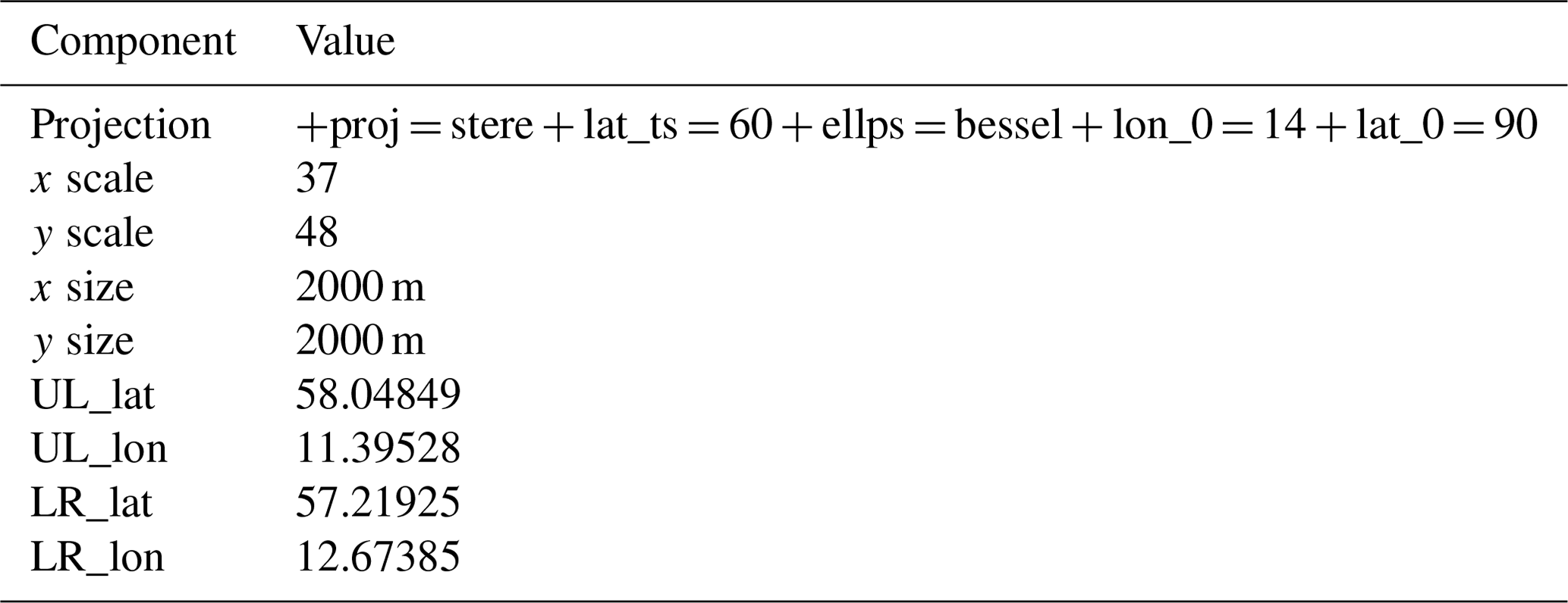
Table 3 Characteristics of radars contributing to the NORDRAD composite.

2.3 Radar

The included radar data set is a subset of one of the operational NORDRAD composite radar products. NORDRAD was the operational radar product at the time for Sweden, and the composite selected is based only on Swedish radars. This subset covers the Gothenburg area, with an extent of around 10 km beyond the maximum extent of the microwave links. The projection parameters of the radar data can be found in Table 2. NORDRAD (Carlsson, 1995) is a set of operational products that are created within a close collaboration between different countries in the Nordic–Baltic region, and more information on NORDRAD can be found in Berg et al. (2016). This composite is created from all available radars at the lowest elevation (0.5^∘). The Gothenburg area is covered by three Swedish radars during this period, i.e. Vara, Karlskrona, and Vilebo. Vara is the closest radar at 78 km. The other two are backups in case Vara does not provide data, but they cover only part of the domain, as the other radars are at their extreme scan ranges. Details of the radar can be found in Table 3. More details of the Swedish radars can be found in Norin (2015). The radar composite is also gauge-corrected by a distance-dependent gauge–radar ratio estimation (Michelson and Koistinen, 2000).

Radar reflectivity (Z) is usually expressed in decibels (dBZ). The data contain radar reflectivity in pseudo-dBZ, meaning dBZ is converted to values between 0 and 255 for efficient storage (255 represents missing data). The data values can be converted back to actual dBZ values with Eq. (2), which is automatically applied when reading the provided netCDF file.

$$\begin{array}{}\text{(2)}& \mathrm{dBZ}=\mathrm{0.4}\cdot \text{value}-\mathrm{30}.\end{array}$$

Equation (3) is needed for conversion of the dBZ to reflectivity Z, as follows:

$$\begin{array}{}\text{(3)}& Z={\mathrm{10}}^{\left(\frac{\mathrm{dBZ}}{\mathrm{10}}\right)}.\end{array}$$

Finally, the rainfall intensity, R (mm h⁻¹), can be found from the following Z–R power law relation in Eq. (4):

$$\begin{array}{}\text{(4)}& Z=a{R}^b,\end{array}$$

where a and b describe the power law coefficient and exponent. The coefficient a is 200, and the exponent b is 1.6 for a standard Marshall–Palmer equation (Marshall et al., 1955). SMHI employs a slightly different exponent value during summer, i.e. b=1.5. The SMHI exponent value is used for the calculations represented in this paper, and its use is also recommended for validation purposes.

3 Methods

The methods employed in this paper focus on presenting the characteristics of the data and the performance of the data collection process. As the gauge data included in the OpenMRG data set are intended to represent the “ground truth”, a limited comparative description is included to highlight key characteristics and some differences. No further in-depth analyses are included, since the main objective of the paper is to share data.

Two approaches were applied to assess the reliability of the data collection. First, we calculated the overall number and percent of time steps for which data were successfully collected for at least one sub-link, rain gauge, or radar pixel compared with the total number of 10 s time steps in the study period. Second, we calculated the data collection hit rate for every sub-link, i.e. the percent and number of time steps with valid data for each specific sub-link relative to all 10 s time steps in the study period. For TSL, we also analysed the stability of the signal by calculating the range (i.e. difference between minimum and maximum TSL) observed across the valid time steps for every sub-link.

Standard descriptive statistics (minimum, maximum, mean, and standard deviation) were derived for each variable, and histograms plotted to show the distribution of the data. Moreover, the rain gauge observations were characterized in terms of the type of descriptive statistics that are commonly used in the analyses of high-resolution rainfall observations, as follows:

• Total rainfall, PTOT. This refers to the total accumulated rainfall over the period (mm).

• Wet fraction, WF^ap. This refers to the fraction of all available time steps having a rainfall amount p≥ 0.1 mm at the aggregation period ap (min).

• Standard deviation, SD^ap. This refers to the standard deviation of the wet fraction depths (i.e. from all time steps with p≥ 0.1 mm) at the aggregation period ap (min).

• Maximum rainfall, PMAX^ap. This refers to the maximum rainfall (mm) at the aggregation period ap (min).

The last three statistics were calculated for aggregation periods (ap) 15 and 1440 min (1 d). In these calculations, the 1 min observations from the City network were firstly aggregated into 15 min time steps, to correspond with the SMHI gauge.

To gain a general overview of the rainfall events that occurred during the study period (JJA 2015), the gauge observations were plotted as time series and cumulative sums. We then analyse a high-intensity event to better understand the correspondence between the gauge, CML, and radar data sets. RSL time series were plotted along with gauge observations as a means of quality control by checking whether the expected behaviour – decreasing RSL levels with increasing rainfall intensity – could be observed. Similarly, the time series of the radar pixel overlying the Torslanda gauge and a set of radar-based maps were plotted to illustrate its correspondence with the gauge and CML data.

4 Results

In this section, we present the results of the data collection and provide some fundamental characteristics of the data. We then plot the rainfall dynamics in the study area during the 2015 summer and illustrate the correspondence between the different sensor observations through an intense rainfall event.

Table 4 Overview of data collection results.

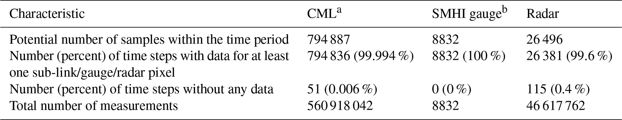
^a For CML, the values refer to valid pairs of RSL and TSL values. ^b Values represent the precipitation gauge at station GbgA.

Figure 6 CML data collection performance. (a) Distribution of the data collection hit rate (percent of time steps with valid RSL and TSL measurements) across all sub-links. In total, 93 % of sub-links have both RSL and TSL data for ≥ 99 % of all time steps in the sampling period. (b) Stability of the transmitted signal level (TSL) across all sub-links. TSL does not vary at all for a majority of the sub-links (68 %).

4.1 Data collection performance

The collection of data from the CMLs, gauges, and radars was generally very successful (Table 4). Overall, 99.99 % of the time steps were monitored by at least one sub-link in the CML network. For 93 % of the sub-links, the data collection was successful ≥ 99 % of the time (Fig. 6a). Of the 728 sub-links, 16 lack either RSL or TSL data for the entire period. Typically, this is a result of failure to access specific nodes (e.g. because of maintenance), and it always affected the same links (i.e. eight links in total). The sporadic missing data at the other sub-links can be caused by a variety of sources, e.g. blockages of the signal to the extent that no received signal was recorded, or due to radio timeout issues. The transmitted signal level (TSL) was constant for a majority of the sub-links (Fig. 6b) because the network was operated without Adaptive Transmit Power Control (ATPC). This stability of the TSL signal facilitates further analysis, since it becomes less sensitive to TSL fluctuations and quantization error. Nevertheless, some effects of the TSL resolution (± 1 dB) are still present in the data, manifested by occasional TSL jumps. These are typically caused by temperature variations (in turn caused by, for example, variations in radio load and air temperature) which are only sometimes captured at the ± 1 dB encoding resolution.

No negative impacts on the CML network operations were observed due to the data collection. The collection load was approximately 10 B s⁻¹ per node on average, and collection from the entire network scaled linearly with the number of nodes sampled (418 × 10 B s⁻¹ = 4180 B s⁻¹), which is very small compared with the total network capacity that is often of the order of 100 Mb s⁻¹ or more. The data could also be collected with a very small time lag. The data collection step took only a few seconds. By design, the system then waited until the entire minute was collected before passing on the data to archive storage and for further processing. Overall, this led to just over a minute in lag between observed event and data available, which is faster than most conventional rainfall monitoring systems. It can clearly be optimized further, but these results already indicate that CMLs are suitable for real-time applications (as demonstrated at https://www.smhi.se/memo, last access: 29 November 2022).

Table 5 Descriptive statistics of the collected CML and radar data. SD refers to standard deviation.

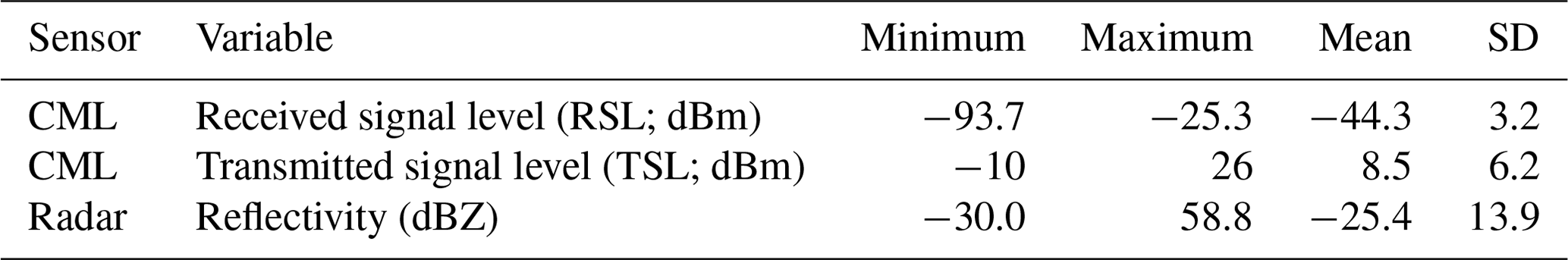
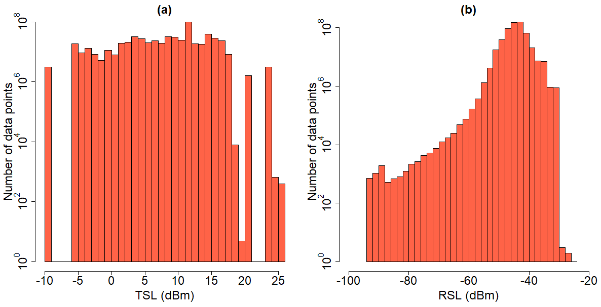
Figure 7 Histograms of (a) transmitted signal level (TSL) and (b) received signal level (RSL). Note that a logarithmic scale is used for the y axis.

The weight-based SMHI gauge GbgA recorded data for 99.95 % of the 15 min intervals in the study period (Table 4), i.e. providing a near-complete record of precipitation events at that location. The completeness of the data collection for the City gauges is not known since they only store data when rainfall occurs (i.e. it is not possible to distinguish zero from missing data). However, the similarity of their records to the SMHI gauge (see below) indicates that the completeness of the City gauge records is likely high. The radar data also display a high completeness, with only about 0.4 % of the potentially available time steps missing data (Table 4). All in all, the data collection was successful, providing near-complete time series for the CMLs, gauges, and radars available in the area.

4.2 Descriptive statistics

Table 5 and Figs. 7 and 8 present the distribution and descriptive statistics of the collected CML and radar data. The TSL measurements have a relatively even distribution, from −6 to 18 dBm, except for a peak at 12 dBm. This reflects the design and authorized operating conditions of the CML network. The RSL measurements are concentrated around the mean, which likely represents the prevalence of dry stable conditions for the vast majority of time steps. Still, there are some significant deviations from the mean, especially at the left tail, which is where the information relevant for rainfall estimation lies (Fig. 7b). To illustrate this, we calculated the difference between the median RSL and the minimum RSL for each sub-link. For the OpenMRG data set, this yields a dynamic RSL range of about 30 dB on average (varying between 0 and 54.6 for individual sub-links). This variability stems from a range of factors, of which signal attenuation due to rainfall is one of the most important. At very low RSL (below approximately −90 dBm), no signal remains, and what is recorded is only sporadic noise. This is reflected in the elevated number of data points at the far left of the histogram.

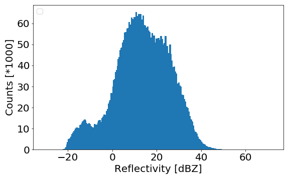
Figure 8 Histogram of radar reflectivity (dBZ). Note that the counts of the minimum values at −30 dBZ (representing the lowest measured reflectivity) were removed (i.e. 41 691 984 counts).

Table 6 Key rainfall statistics for the rain gauge observations during June–August 2015. For gauge locations, see Fig. 2.

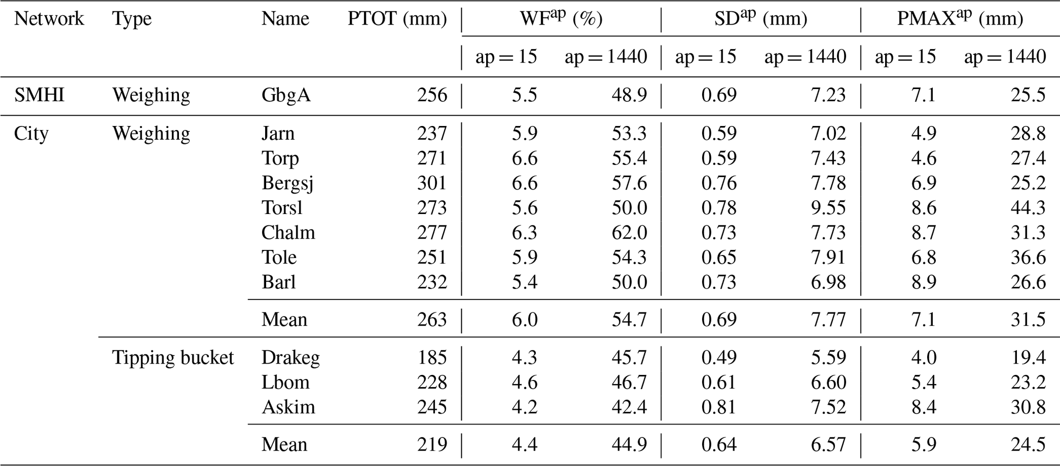
Figure 8 and Table 5 provide basic statistics and a histogram of the reflectivity distribution in dBZ for the entire radar data set (all data points contained in the data set). As can be seen, there are few reflectivities that are above 40 dBZ, which is a common threshold for convective precipitation (Steiner et al., 1995). It is also interesting to note the small peak around −15 dBZ, which might be caused by clutter. The minimum value in Table 5 of −30 dBZ represents the lower limit of the measured reflectivity by the radar. As a general guide, all values below 0 dBZ could be considered to be zero rainfall. This corresponds to around 0.03 mm h⁻¹, using the SMHI Z–R relation. The low mean illustrates the high amount of zero precipitation.

Table 6 provides key descriptive statistics for all rain gauge observations. Based on a limited climatological analysis of observations since 1996 (not shown), it has been found that the period under study (JJA 2015) overall represents an “average summer” well with respect to rainfall in Gothenburg, although the maximum values (PMAX) are somewhat on the low side. Looking first at total rainfall during the period, PTOT, it is 256 mm in the SMHI gauge. The mean value from the weighing stations in the City network (263 mm) is very close to the SMHI gauge, indicating that the SMHI gauge well represents the city in aggregate terms, as also suggested in Fig. 10. The tipping-bucket gauges, however, have a distinctly lower mean value (219 mm), which may be caused by, for example, shielding and excessive undercatch due to suboptimal placement, evaporation losses, or occasional clogging. Much of the difference can be attributed to single periods with high-intensity rainfall affecting only parts of the city.

At the accumulation period (ap) 15 min, the wet fraction (WF) in the SMHI gauge is 5.5 %. Whereas the weighing gauges in the City network generally have a slightly higher WF, the WF for the tipping-bucket gauges are distinctly lower. The highest WF value among the tipping-bucket gauges (4.6 %) is almost 1 percentage point lower than the lowest WF value among the weighing gauges (5.4 %). In the SMHI gauge WF¹⁴⁴⁰ = 48.9 %, i.e. it rained on average every second day. Also, in this case, WF is higher for the weighing gauges in the City network and distinctly lower for the tipping-bucket gauges. In the City network, overall the WF values at different accumulation periods are similarly ranked, i.e. a high value at ap = 15 min implies a high value also at ap = 1440 min, although minor deviations from this pattern exist.

In the SMHI gauge, the standard deviation SD ranges from 0.69 mm at 15 min to 7.23 mm at the 1440 min accumulation period. These values are overall well matched by the City network gauges, regardless of type. In the SMHI gauge, the maximum value PMAX¹⁵ = 7.1 mm and PMAX¹⁴⁴⁰ = 25.5 mm. Also, these values are well matched overall by the City network gauges. A distinct spatial variation in the seasonal maximum values is expected, particularly at short durations, considering the small-scale convective rainfall processes that are generally involved in generating these extremes.

Figure 9 Rainfall time series in the SMHI gauge at 15 min (a) and 1 d (b) temporal resolution.

4.3 Rainfall dynamics during summer 2015, as observed by the gauges

Figure 9 shows the time series plots of rainfall in the SMHI gauge during the study period (JJA 2015). The highest 15 min accumulations (up to 6–7 mm) were recorded on 28–29 July, but the highest daily accumulation (25.5 mm) was on 17 June. Whereas the former event was dominated by isolated very high 15 min intensities, the daily maximum was caused by a nearly 10 h long low-intensity event. Several short high-intensity events occurred surpassing the national 1 min cloudburst threshold of 1 mm (e.g. 9 times at station Bergsj), although no events were recorded surpassing the national 1 h cloudburst threshold (50 mm in 1 h).

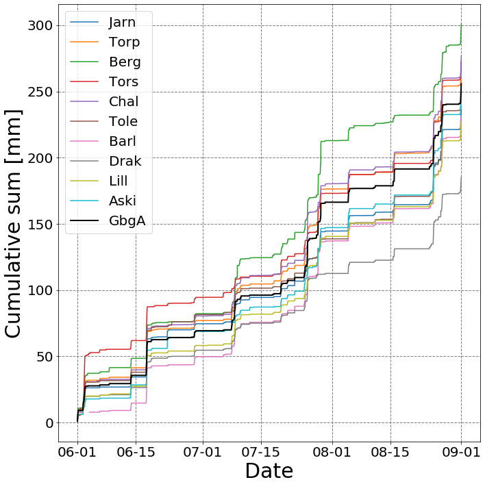
Figure 10 Comparison of the SMHI gauge and the City network gauges. The figure shows the cumulative rainfall sum in each gauge over the study period.

The cumulative sum during the period shows that the rainfall in the City network gauges (i) follows the pattern in the SMHI gauge well and (ii) is rather evenly distributed around the SMHI gauge (Fig. 10). Differences in rainfall during two periods are responsible for most of the spread between the gauges, namely the first one on 1–2 June and the second one on 28–29 July. Both periods were characterized by large spatial variability, with some gauges recording only a few millimetres and others up to 50 mm.

Figure 11 (a) An intense rainfall event at the Torslanda gauge on 28 July 2015, (b) the corresponding RSL signal fade for a nearby microwave link (link 10227 and sub-links 115 and 118), and (c) the reflectivity of the overlying radar pixel. The locations of the gauge and link are shown in Fig. 12. Sub-link 115 is vertically polarized, with a frequency of 28.23 GHz, covering a 1.8 km distance. Sub-link 118 is identical, except for operating at 29.24 GHz. An interactive version of this figure is available together with the data set (see Sect. 6).

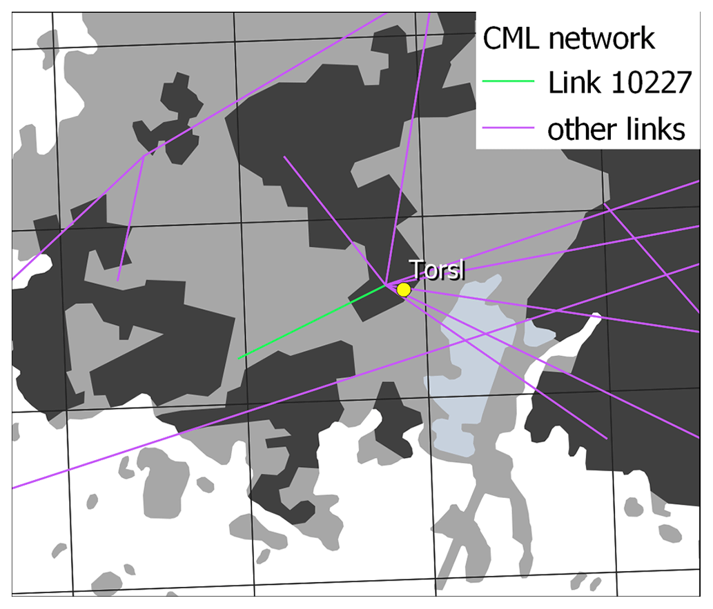
Figure 12 Map of the Torslanda gauge (Torsl) and surrounding CMLs, with link 10227 highlighted, as used in Fig. 11.

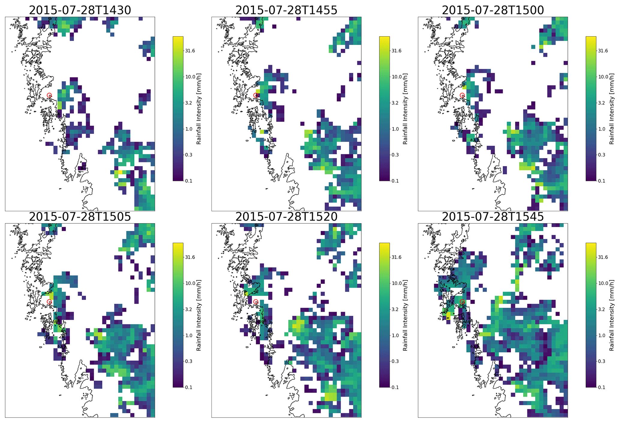
Figure 13 Estimated rainfall intensity based on the radar data at key time steps during 28 July 2015. The red circle indicates the location of the Torslanda gauge.

4.4 Case study: the high-intensity event on 28 July 2015

The intense rainfall event recorded on 28 July at Torslanda (Figs. 2 and 12) serves to illustrate the strong correspondence between gauge and CML data. The event lasted for 2 h, with a peak 1 min intensity of 1.1 mm min⁻¹ and a total accumulation of 18.5 mm. The expected behaviour is that received signal level (RSL) will decrease when rainfall intensity increases, and vice versa (ITU, 2005). This was observed on many occasions and is here illustrated during 28 July (Fig. 11). The event also serves to illustrate how radar data are useful for mapping the overall spatial pattern of an event but sometimes fail to represent the local details observed on the ground (Figs. 13 and 11). Before the event (14:30 to 14:55; all times here and below are in UTC), rainfall intensity at the gauge and radar is zero, and the RSL range is small (around −46.5 ± 0.5 dB). The first gauge record of the event is between 14:58 and 14:59, while the sub-links record the first RSL decrease at 14:57:20. The small difference in time is likely caused by the movement of the storm coupled with the difference in geographic position and monitored area of the links and the gauge. At this time, the radar indicates zero rainfall at Torslanda but also some rainfall a few kilometres away. The peak intensity (1.1 mm min⁻¹) is recorded between 15:04 and 15:05 at the gauge, while the deepest RSL fade is at 15:06:00. At this stage, the RSL has dropped significantly, about 27 dB down to −73.6 dBm. The intensity then goes down at the gauge, and the RSLs follow suit by increasing again toward their starting values. During this peak, the radar indicated that no rainfall occurred at the grid cell overlying Torslanda but also that some higher-intensity rainfall occurred several kilometres further north. The reason for the failure of the radar to capture the event at Torslanda is unknown, but it could be due to, for example, spatial misalignment (placing the peak too far north), advection, low temporal sampling frequency (one snapshot every 5 min), or overshoot (giving no echo at Torslanda). Some neighbouring radar grid cells display elevated reflectivities around 15:05, which suggests horizontal and/or vertical misalignment is the most likely cause in this case. At 15:22, the gauge again reports zero rainfall, while at the same time the RSL recession is still ongoing (i.e. RSL is still not back to the initial pre-event levels). This is likely an effect of wet-antenna attenuation, difference in geographic position, or the spatially integrated nature of CMLs (recording signal fluctuations across the entire link path). What then follows is a lighter shower peaking at 15:45, which is observed by the gauge, the CMLs, and the radar. At the end of this, the gauge displays a jerky behaviour with alternating records of 0 and 0.1 mm min⁻¹. This is probably a result of the measurement resolution of the gauge. The CML data here provide a smoother representation, which is more realistic.

In general, the sub-links display similar temporal dynamics to the gauges, but there are also exceptions. For example, the last peak observed at Torslanda during this event (0.7 mm min⁻¹ at 16:22; Fig. 11) resulted in a smaller RSL drop when compared with the same intensity during the first peak. One potential reason could be differences in the spatial alignment between the location of the most intense rainfall and the gauge and sub-link locations, respectively, for the two events. Another reason could be that the antenna was wetter during the first peak than during the second, resulting in less wet-antenna attenuation during the second peak. The open publication of this data set provides a good opportunity to further analyse the correspondence between RSL dynamics, gauges, and radar more comprehensively.

5 Discussion

The above comparative description of rain gauge observations in Gothenburg during summer 2015 well illustrates the very high spatial and temporal small-scale variability in rainfall, also found in numerous other studies worldwide (e.g. Krajewski et al., 2003). Consequently, accurate observation requires very high resolutions in space and time, and CML networks offer a unique possibility of performing such high-resolution observations. A key advantage is that the CML infrastructure is already in place; the number of operational CML hops in Sweden is more than 20 000, in Europe there are more than 400 000, and several millions exist globally (Ericsson, 2018).

The primary intended use of the OpenMRG data set is to allow a wider research community to develop and refine algorithms for rainfall retrieval from CML networks. A number of data processing challenges have been identified. The first set of challenges concern separating rainfall information from other factors affecting the microwave signal, such as refractivity-induced multipath fading, wet-antenna attenuation, intermittent disturbances due to human activities (e.g. construction cranes, ferry crossings, and maintenance), canopy foliage dynamics, antenna misalignments, multipath fading over waterbodies, random noise, etc. (Bao et al., 2017). Several of these factors are also present in the OpenMRG data set (visible, for example, in RSL jumps, diurnal cycles, high-frequency oscillations, and the delayed return to baseline conditions). A second set of challenges concern estimating rainfall intensities accurately for links with different frequencies, polarization, lengths, temporal resolution, signal quantization, and unstable baseline conditions and operating in different climatic, physiographic, and management conditions. A third category of challenges concerns the integration of different links and potentially also gauges, radars, and other information sources into high-resolution maps and spatiotemporally complete data sets. Significant progress has been made by a number of research groups on many of these challenges over the past decade. Conceivably, the extensive data included in the OpenMRG data set will make it possible to further improve our capacity to meet these challenges and to help scrutinize the general applicability of existing methods.

There are several applications of up-to-date high-resolution rainfall data. One key application is the real-time mapping of current and past events, which are used, for example, in operational meteorological forecasting, model evaluation, and post-event insurance analyses. CML networks can be used to create near-real-time high-resolution rainfall maps, as demonstrated at https://www.smhi.se/memo (last access: 29 November 2022). Another key potential application is hydrological modelling and forecasting, as demonstrated by, for example, Fencl et al. (2013). Frequent initialization of the hydrological model, i.e. model state update to reflect current hydrological conditions, is crucial for accurate performance (Hapuarachchi et al., 2011). Furthermore, hydrological response to rainfall always has a delay, which may be days or weeks in large rural basins but below 1 h in small urban basins. Using the most recent rainfall observations is thus a very fundamental prerequisite for accurate hydrological forecasts. Considering the particularly dense CML networks in cities, urban applications are of obvious significance, such as for the real-time control of sewer systems for quantitative and qualitative water management, but also rural hydrological forecasting in poorly or ungauged regions is a motivating prospect. These possibilities are already being explored (e.g. in Stockholm; von Scherling et al., 2021), and the open sharing of OpenMRG aims to further such research and applications.

6 Data availability

The OpenMRG data set is openly available at https://doi.org/10.5281/zenodo.7107689 (Andersson et al., 2022) under the Creative Commons Attribution Share Alike 4.0 licence. More details on the data structure and files are provided in the data repository. The OpenMRG data covers the period June–August 2015. More data for the GbgA station are available at https://opendata.smhi.se/ (last access: 29 November 2022) (specifically, https://opendata-download-metobs.smhi.se/explore, last access: 29 November 2022). In addition to the data, we also include scripts to read the data, an interactive version of Fig. 11, and a radar animation covering the 2015 event at Torslanda (Fig. 13).

7 Concluding remarks

Technical development, e.g. information technology and digitalization, occasionally brings unexpected and unintentional opportunities for additional benefits. Rainfall monitoring through processing of microwave network signals is a good example of such an opportunity. Although development remains in terms of both data handling and conversion algorithms, the step to large-scale and widespread operational monitoring using CMLs is relatively small from a technical perspective, since the infrastructure is essentially already in place. Rather, the main challenge to overcome concerns enabling access to CML data. Key to this endeavour is to develop mutually beneficial collaborations and viable business models involving key actors, such as mobile network operators, CML manufacturers, hydrometeorological agencies, municipalities, and researchers. It is our hope that rainfall monitoring by CML networks will soon reach widespread operational implementation and thereby provide a distinct added value in a sustainable and climate-proof society.