A high-resolution Antarctic grounding zone product from ICESat-2 laser altimetry

The Antarctic grounding zone, which is the transition between the fully grounded ice sheet to freely floating ice shelf, plays a critical role in ice sheet stability, mass budget calculations, and ice sheet model projections. It is therefore important to continuously monitor its location and migration over time. Here we present the first ICESat-2-derived high-resolution grounding zone product of the Antarctic Ice Sheet, including three important boundaries: the inland limit of tidal flexure (Point F), inshore limit of hydrostatic equilibrium (Point H), and the break in slope (Point I_b). This dataset was derived from automated techniques developed in this study, using ICESat-2 laser altimetry repeat tracks between 30 March 2019 and 30 September 2020. The new grounding zone product has a near-complete coverage of the Antarctic Ice Sheet with a total of 21 346 Point F, 18 149 Point H, and 36 765 Point I_b locations identified, including the difficult-to-survey grounding zones, such as the fast-flowing glaciers draining into the Amundsen Sea embayment. The locations of newly derived ICESat-2 landward limit of tidal flexure agree well with the most recent differential synthetic aperture radar interferometry (DInSAR) observations in 2018, with a mean absolute separation and standard deviation of 0.02 and 0.02 km, respectively. By comparing the ICESat-2-derived grounding zone with the previous grounding zone products, we find a grounding line retreat of up to 15 km on the Crary Ice Rise of Ross Ice Shelf and a pervasive landward grounding line migration along the Amundsen Sea embayment during the past 2 decades. We also identify the presence of ice plains on the Filchner–Ronne Ice Shelf and the influence of oscillating ocean tides on grounding zone migration. The product derived from this study is available at https://doi.org/10.5523/bris.bnqqyngt89eo26qk8keckglww (Li et al., 2021) and is archived and maintained at the National Snow and Ice Data Center.

1 Introduction

With a global sea level rise equivalent of 58 m (Fretwell et al., 2013), the Antarctic Ice Sheet has been losing ice at an accelerated pace (Shepherd et al., 2018). This mass loss is largely driven by the ice dynamics of the marine ice sheet due to sustained and accelerated thinning of the ice shelves (Bamber et al., 2009; Paolo et al., 2015; Pattyn and Morlighem, 2020; Favier et al., 2014; Gardner et al., 2018) and rapid retreat of the grounding line (hereinafter referred to as the GL) (Point G in Fig. 1) (Christie et al., 2018; Milillo et al., 2019; Rignot et al., 2014; Scheuchl et al., 2016), which is the boundary between the grounded ice sheet and the floating ice shelves (Rignot et al., 2011a). The grounding line is identified as an essential climate variable that is critical in understanding Earth's climate by the Global Climate Observing System. Knowledge of its location is important in ice sheet numerical modelling and mass budget estimation as it controls the rates of ice flux from the grounded ice sheet into the ocean (Schoof, 2007), and it is a key indicator of the marine ice sheet instability (DeConto and Pollard, 2016; Joughin et al., 2014; Ritz et al., 2015). Therefore, continuous long-term monitoring of the GL location and its temporal migration is crucial for understanding ice sheet stability and assessing the Antarctic Ice Sheet's contribution to future sea level rise.

Figure 1 Schematic diagram of the ice shelf grounding zone (GZ) structure adapted from Fricker and Padman (2006). Point G is the true grounding line where the grounded ice first comes into contact with the ocean, Point F is the landward limit of ice flexure caused by ocean tidal movement, Point H is the seaward limit of ice flexure and the inshore limit of hydrostatic equilibrium, Point I_b is the break in surface slope, and Point I_m is the elevation minimum inside the GZ.

The GL is located inside the grounding zone (hereinafter referred to as the GZ; Fig. 1). The GZ is defined as the region between the landward limit of tidal flexure (Point F in Fig. 1), where the ice is not influenced by ocean tides, and the inshore limit of hydrostatic equilibrium (Point H in Fig. 1) where the ice is floating in full hydrostatic equilibrium (Brunt et al., 2010b; Fricker and Padman, 2006). Inside the GZ, there is often a surface elevation minimum (Point I_m in Fig. 1) and an inflection point in ice surface slope where the slope changes most rapidly (Point I_b in Fig. 1) (hereinafter referred to as the break in slope). As the GL is a subglacial feature, it is difficult to directly identify from in situ measurements or satellite observations (Horgan and Anandakrishnan, 2006). Instead, previous methods used satellite-observable GZ features (Points F and I_b) as proxies for the GL (Brunt et al., 2010b). Additionally, Point H is usually mapped as it can provide a measure of the GZ width and is valuable in calculating ice thickness based on hydrostatic equilibrium (Dawson and Bamber, 2020; Rignot et al., 2011a).

There are two established approaches for estimating the GL location using remote sensing techniques: (a) directly detect the break in slope (hereinafter referred to as the “static method”); (b) use observations of surface elevation change due to variations in ocean-tide-induced tidal flexure (hereinafter referred to as the “dynamic method”). The break in slope is mapped by identifying the inflection of the ice surface slope from a digital elevation model (DEM) (Brunt et al., 2010b, 2011; Fricker and Padman, 2006; Hogg et al., 2018; Horgan and Anandakrishnan, 2006) or the change in brightness in satellite optical imagery (Bindschadler et al., 2011; Christie et al., 2016, 2018). The satellite-optical-imagery-based approaches are able to provide complete coverage of the Antarctic Ice Sheet (Bindschadler et al., 2011; Scambos et al., 2007). However, they work best only when the ice thickness increases rapidly inland from the GZ and often fail to map the GL in areas of fast ice flow where the subglacial bed and surface slope are shallow (Christie et al., 2016, 2018).

Repeat-track and crossover analysis of satellite altimetry (Brunt et al., 2010b, 2011; Dawson and Bamber, 2017, 2020; Fricker and Padman, 2006; Li et al., 2020) and differential synthetic aperture radar interferometry (DInSAR) (Brancato et al., 2020; Mohajerani et al., 2021; Rignot et al., 2016; Rignot, 1998; Scheuchl et al., 2016) use the dynamic method to detect Points F and H. In general, DInSAR has been the most successful method of capturing Point F accurately and providing overall good spatial coverage. However, there are relatively few regions that have been measured repeatedly by DInSAR (Friedl et al., 2020; Hogg et al., 2018), while some areas have not been mapped at all due to orbital limitations of the satellites (Mohajerani et al., 2018). Satellite altimetry, therefore, can provide valuable information where DInSAR measurements are not available. The existing satellite-altimetry-derived GZ products from ICESat (Brunt et al., 2010a) and CryoSat-2 (Dawson and Bamber, 2020) suffer from poor temporal and spatial coverage and are not suitable to monitor changes in the GZ. ICESat-2, launched on 15 September 2018, however, has higher along-track resolution and better spatial coverage compared with ICESat (Markus et al., 2017). It can be used to map the Antarctic GZ with greater accuracy and spatio-temporal coverage than previous satellite-altimetry-derived products. Here we generated the first ICESat-2-derived Antarctic GZ product with high spatio-temporal coverage using 18 months of ICESat-2 laser altimetry data (Li et al., 2021), including three GZ features: Points F, H, and I_b. This will be a valuable resource for comparison with other methods and can provide high-resolution GZ coverage in regions where DInSAR measurements of Point F are not available (either spatially or in time). The new dataset also provides state-of-the-art knowledge of GZ locations and is useful in understanding Antarctic Ice Sheet instability.

This paper provides a detailed description of the ICESat-2-derived GZ product and the methodologies used to derive the dataset. We also discuss the associated uncertainties and validate the new GZ product with ICESat-2 crossover measurements and previous GZ products.

2 Data and methodology

2.1 ICESat-2 data and processing

ICESat-2 measures the ice sheet surface elevation at a repeat cycle of 91 d. The Advanced Topographic Laser Altimeter System (ATLAS) onboard ICESat-2 has three beam pairs in comparison with the single beam of the Geoscience Laser Altimeter System (GLAS) onboard ICESat. The across-track spacing between each beam pair is approximately 3.3 km, with a pair spacing of 90 m. The along-track sampling interval of each beam is 0.7 m with a nominal 17 m diameter footprint (Markus et al., 2017; Smith et al., 2019).

In this study, we used version 3 of the ATL06 Land Ice Along-Track Height Product (Smith et al., 2019) from 30 March 2019 to 30 September 2020 (Scheick et al., 2019; Smith et al., 2020a) to map three different GZ features, including the landward limit of tidal flexure (Point F), the inshore limit of hydrostatic equilibrium (Point H), and the break in slope (Point I_b) (Fig. 1). The ATL06 elevation is calculated by averaging individual photon data over 40 m length segments with an along-track resolution of 20 m (Smith et al., 2019); the elevation accuracy is estimated to be better than 3 cm (Brunt et al., 2019). There are seven repeat cycles (3–9) in the study period, among which, cycles 4 and 9 are not complete.

We processed the ATL06 elevation data using the same methods described in Li et al. (2020). We did not apply the ocean tide correction to ICESat-2 ATL06 elevation, and we “re-tided” the ocean loading tide. Poor-quality elevation measurements caused by clouds or background photon clustering were removed by applying the ATL06_quality_summary flag (Smith et al., 2019). A neighbouring surface elevation consistency check was applied by using the along-track slope of each ground track. We only kept elevation measurements where differences between the original elevations and the estimated elevations from along-track slope were lower than 2 m. The reference segment locations of each ground track were also derived from the “segment_quality” group to calculate a reference track, which will later be used in the GZ calculation.

2.2 Repeat-track preparation

Our method of estimating GZ features utilizes ICESat-2 repeat tracks from different cycles (Fig. 2, Box 1). Following the steps of repeat-track generation described in Li et al. (2020), the surface elevation, elevation measurement geolocations, and the reference segment geolocations of 6 ground tracks along each of the 1387 reference ground tracks (RGTs) were categorized into 9 distinct repeat-track data groups, including 6 single-beam repeat-track data groups and 3 beam pair repeat-track data groups (Fig. 4a and b in Li et al., 2020). For each repeat-track data group, a “nominal reference track” was calculated by averaging the locations of reference segments from all repeat tracks inside this data group. A reference GL was also calculated as the intersection between the nominal reference track and a composite GL which was generated by merging the Depoorter et al. (2013) GL with the most recent GLs from different sources (Table A1). Allowing for a possible GL change between the current GZ location and the composite GL, we defined a 15 km calculation window landward and seaward of the reference GL along the nominal reference track; only ATL06 elevation measurements located within this calculation window were used in the GZ calculation (Li et al., 2020). This is to ensure the pre-defined calculation window can capture the GZ adequately in our study period due to potential GL changes during the past decade, especially for the fast-flowing glaciers.

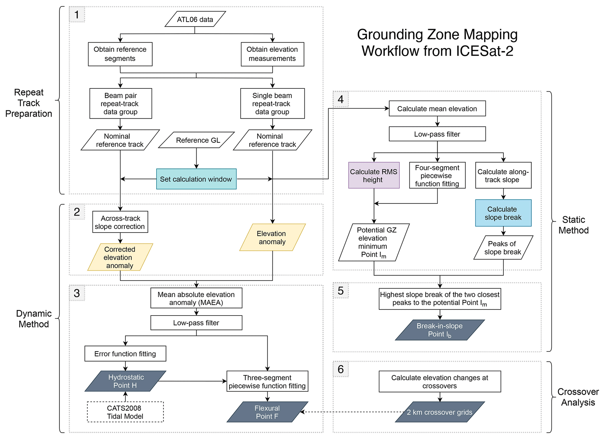
Figure 2 The automatic workflow of identifying the grounding zone (GZ) features from ICESat-2 data. Box 1: ICESat-2 repeat-track preparation; Boxes 2 and 3: estimation of the landward limit of tidal flexure (Point F) and the inshore limit of hydrostatic equilibrium (Point H) from the dynamic method; Boxes 4 and 5: estimation of the break in slope Point I_b from the static method; Box 6: ICESat-2 crossover analysis. Grey parallelograms denote the grounding zone features. Boxes with other colours denote key steps in the GZ estimation.

We removed ATL06 data points with elevation higher than 400 m and data points located in open water based on the coastline mask provided in the SCAR Antarctic Digital Database (ADD) (https://data.bas.ac.uk/items/ed0a7b70-5adc-4c1e-8d8a-0bb5ee659d18/, last access: 6 July 2020) to only include data in the GZ. We also only included repeat tracks inside the calculation window where at least 50 % of the elevation measurements are valid as any track where fewer than 50 % of the data were valid was regarded as insufficient for GZ calculation and was removed.

2.3 Dynamic method: identify the limits of tidal flexure

The key feature of the dynamic method is to identify the temporal changes in ice surface elevation due to ocean tides between Points F and H from different repeat tracks (Brunt et al., 2010b, 2011; Fricker and Padman, 2006). The temporal ice surface elevation changes were derived from a set of “elevation anomalies” (Fig. 2, Box 2). For each single-beam repeat-track data group, the reference elevation profile along the nominal reference track was first calculated by averaging the elevations of each repeat track at the nominal reference track; then elevation anomalies were calculated by differencing the elevation profile of each individual repeat track and this reference elevation profile (Li et al., 2020) (Fig. 3c, h, m). For the beam pair repeat-track data group, the elevation profile of each individual repeat track was first corrected for the across-track slope onto the nominal reference track (Eqs. 1 and 2 in Li et al., 2020). The average of all across-track slope-corrected elevations from each track at the nominal reference track was then taken as the reference elevation profile. The elevation anomalies were calculated by subtracting this reference elevation profile from the across-track slope-corrected elevation profile of each repeat track inside the beam pair repeat-track data group.

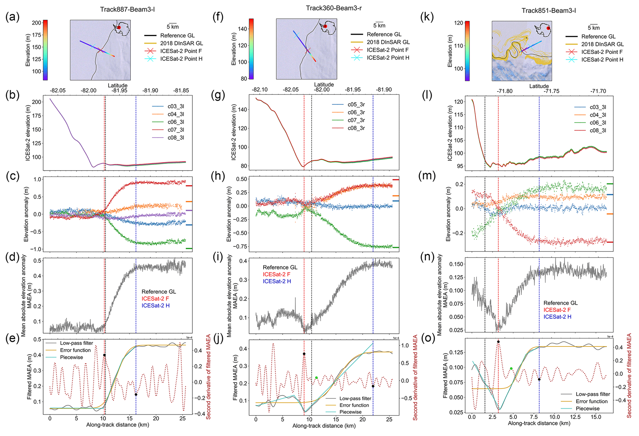
Figure 3 Examples of repeat-track analysis for track 887 (a–e) and track 360 (f–j) on the Filchner–Ronne Ice Shelf and track 851 (k–o) on the Amery Ice Shelf. (a, f, k) The locations of ICESat-2-derived inland limit of tidal flexure Point F (red cross) and the inland limit of hydrostatic equilibrium Point H (cyan cross), along with the reference elevation of the nominal reference track (colour-coded), the composite grounding line (GL) (black line) used to calculate the reference GL in the repeat-track analysis, and the DInSAR-derived Point F in 2018 (yellow line) (Mohajerani et al., 2021). All data are overlaid on the Landsat Image Mosaic of Antarctica (Bindschadler et al., 2008). (b, g, l) ICESat-2 “re-tided” elevation profiles. (c, h, m) The elevation anomalies of all repeat tracks inside each repeat-track data group. The horizontal lines at the right are the zero mean tide height predictions from the CATS2008 tidal model (Padman et al., 2002). (d, i, n) The mean absolute elevation anomaly (MAEA). (e, j, o) Low-pass-filtered MAEA is shown as a solid grey line; error function fitting of the MAEA is shown as a solid yellow line, the three-segment piecewise function fitting of the landward part of the Point H of the MAEA is shown as a solid green line; the second derivative of low-pass-filtered MAEA is shown as a dotted maroon line; the piecewise-function-derived Point F is shown as the black dot on the left; the wrong Point F picks from error function fitting are shown as the green dots in (j) and (o); Point H is shown as the black dot on the right of each panel. Locations of Point F, Point H, and the reference GL are marked as the vertical dashed red line, vertical dashed blue line, and vertical dashed black line in all panels apart from (a), (f), and (k).

The estimation of GZ features Points F and H are based on extracting the transition points from the mean absolute elevation anomaly (MAEA) (Fig. 3d, i, n), which is defined as the average of the absolute value of all elevation anomaly profiles. The inland limit of tidal flexure, Point F, is identified as the point where the elevation anomaly of each repeat track exceeds a noise threshold (Brunt et al., 2010b, 2011; Fricker et al., 2009). The region where the MAEA is close to zero is regarded as the fully grounded ice (the region to the left of Point F in Fig. 1) as it is not influenced by tidal motion. Point F was then estimated to be the point where the gradient of the MAEA first increases from zero, and the second derivative of the MAEA reaches its positive peak (Li et al., 2020). The inshore limit of hydrostatic equilibrium, Point H, is identified as the location where the elevation anomaly of each repeat track reaches its maximum and becomes stable. It was estimated as the transition point where the gradient of the MAEA finally decreases to zero, and the second derivative of the MAEA reaches its negative peak (Li et al., 2020).

To select the correct transition points from the second derivative of the MAEA curve as Points F and H, previously we used an error function fit to the MAEA as a guide (Li et al., 2020). While the error function can reliably estimate Point H because the gradient of the elevation anomaly always changes smoothly to zero, it is unreliable in identifying Point F where there is a sharp transition on the MAEA curve, or the across-track slope-related noise on land ice is high (green dots in Fig. 3j and o). To solve the inaccurate picks of Point F under these circumstances, instead of using error function fitting, we used a three-segment piecewise function fitting only to the landward part of the Point H on the MAEA profile (Fig. 2, Box 3) (green lines in Fig. 3e, j, o). The closest positive peak of the second derivative of this piecewise function to the reference GL was taken as a guide point to find Point F. As a final step, all results are visually inspected due to the complex nature of the GZs, and ICESat-2 crossover measurements are used as a reference on the Filchner–Ronne and Ross ice shelves (Sect. 2.5). In the final GZ product, we also recorded the number of repeat cycles used and the ocean tide range calculated as the maximum elevation anomaly deviation from all repeat tracks at Point H.

2.4 Static method: identify the break in slope

The break in slope Point I_b and elevation minimum Point I_m are the points where the slope changes most rapidly and where the slope is zero inside the GZ (Bindschadler et al., 2011), respectively. Previous studies using ICESat laser altimetry selected the break in slope by hand (Brunt et al., 2010b; Fricker and Padman, 2006); however given the increased data volume available for ICESat-2, this manual approach is no longer feasible. Here we developed an automated technique to select the break in slope (Fig. 2, Boxes 4 and 5) by solving the problem of complex surface morphologies of the GZ, such as crevasses and ice plains, which used to impose difficulty in interpreting the break in slope (Brunt et al., 2010b, 2011; Fricker et al., 2009; Horgan and Anandakrishnan, 2006). We only used the single-beam repeat-track data groups to determine the break in slope since we do not need to calculate elevation changes between repeat tracks, which can be influenced by across-track slope-induced errors.

The break in slope Point I_b is often associated with a local topographic minimum Point I_m inside the GZ (Brunt et al., 2010b). According to this, we first estimated the potential Point I_m using the along-track rms height R and then used this potential Point I_m to derive the break in slope Point I_b. The rms height of the along-track topography, also referred to as the standard deviation in the elevation, has proven to be a robust way of estimating the surface roughness at a finer scale (Cooper et al., 2019). It is more sensitive to identifying the local topographic extremes compared with using the reference elevation profile itself.

After obtaining the reference elevation profile on the nominal reference track of each single-beam repeat-track data group (Fig. 4b, h, n), we first linearly interpolated the reference elevation based on sequential segments at an along-track distance of 20 m to fill the data gaps (cyan lines in Fig. 4c, i, o). To remove noise caused by small-scale topographic features such as crevasses, we applied a Butterworth low-pass filter with a normalized cut-off frequency of 0.032 and an order of 5 to the interpolated reference elevation profile (black lines in Fig. 4c, i, o). The low-pass filter removed the high-frequency noise without changing the shape of the reference elevation profile, therefore retaining the locations of GZ features.

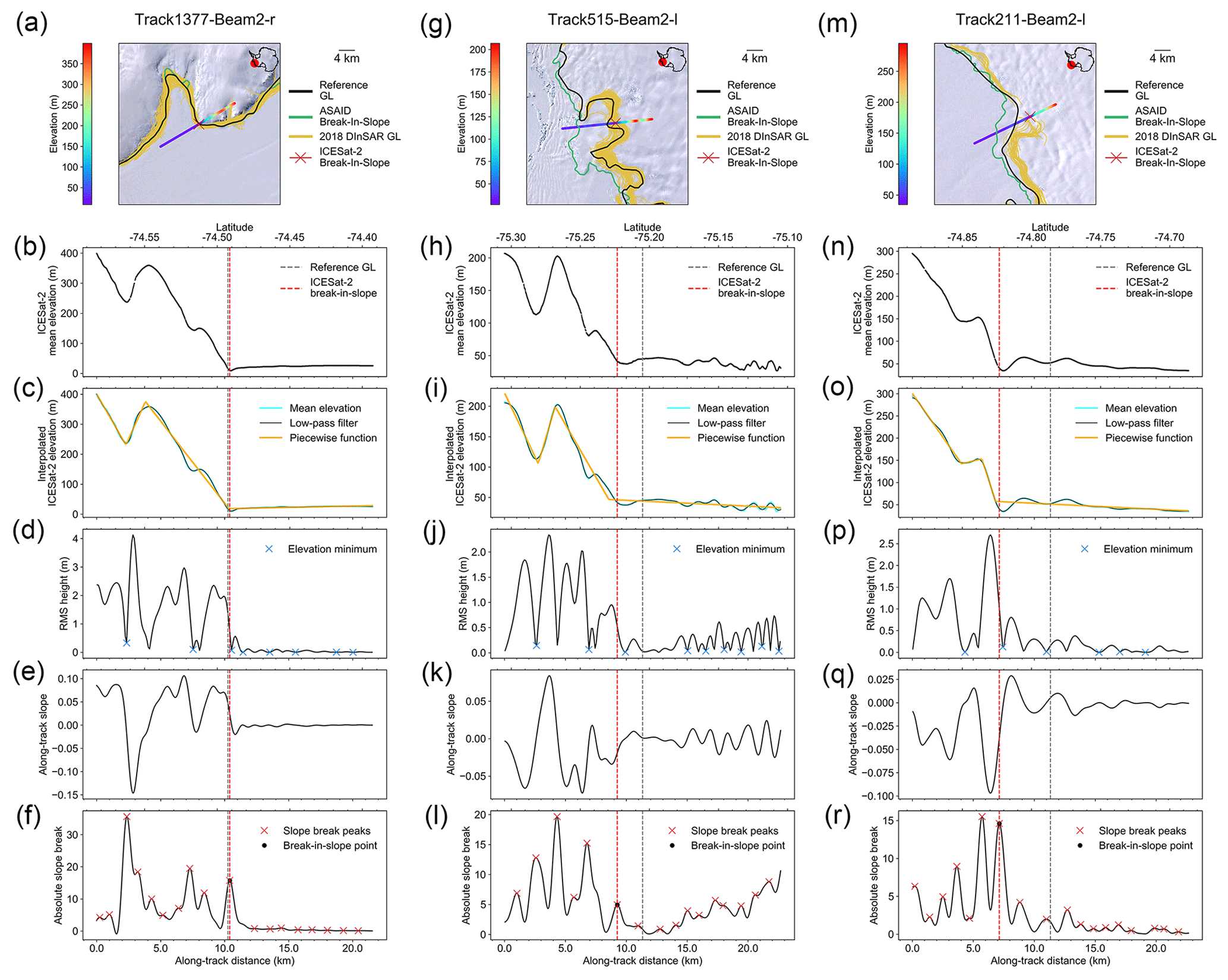
Figure 4 Estimation of break in slope (Point I_b) from ICESat-2 repeat tracks on the Amundsen Sea embayment. (a–f) Track 1377 on Bear Peninsula, (g–l) track 515 in the “butterfly” region of Thwaites Glacier, (m–r) track 211 on an unnamed glacier of Getz Ice Shelf. Geolocations and elevations of ICESat-2 elevation profiles for three different ground tracks are shown in (a), (g), and (m) superimposed on the Landsat Image Mosaic of Antarctica (Bindschadler et al., 2008); the reference grounding line (GL) is shown as a black line, the ASAID break in slope is shown as the green line (Bindschadler et al., 2011); the Sentinel-1a/b DInSAR-derived GL is shown as the yellow line (Mohajerani et al., 2021); the ICESat-2-derived break in slope is shown as a red cross. (b, h, n) The reference elevation profile along the nominal reference track. (c, i, o) The interpolated reference elevation profile is shown as the solid cyan line; the low-pass-filtered interpolated reference elevation profile is shown as the solid black line; the four-segment piecewise function fitting is shown as the solid yellow line. (d, j, p) The along-track rms height of the reference elevation profile; local elevation minima are shown as the blue crosses. (e, k, q) The along-track slope of the reference elevation profile. (f, l, r) The absolute slope break along the reference elevation profile; peaks of the slope break are shown as red crosses, and the final break in slope Point I_b is shown as the black dot. Locations of Point I_b and the reference GL are marked as the vertical dashed red line and the vertical dashed black line in all panels apart from (a), (g), and (m).

We calculated the along-track rms height R with a bin size of 100 m (five elevation measurements) of the low-pass-filtered reference elevation profile using Eq. (1) (Cooper et al., 2019),

$$\begin{array}{}\text{(1)}& R={\left[{\displaystyle \frac{\mathrm{1}}{n-\mathrm{1}}}{\sum }_{i=\mathrm{1}}^n\left(z\right(x_i)-\stackrel{\mathrm{‾}}{z}{)}^{\mathrm{2}}\right]}^{\frac{\mathrm{1}}{\mathrm{2}}},\end{array}$$

where n is the number of sample elevation points, z(x_i) is the elevation of each point, and $\stackrel{\mathrm{‾}}{z}$ is the average elevation of all data points in the calculation window. R is given for the mid-point of each calculation window. The examples of the along-track rms height for three different tracks located in the Amundsen Sea embayment are shown as black lines in Fig. 4d, j, and p. The negative peaks of rms height with a value less than 0.5 m were taken as local topographic extremes. They were further filtered to only keep the elevation minima based on the elevation peaks of the reference elevation profile. To find the potential Point I_m, we first fitted a four-segment piecewise function to the reference elevation profile (yellow lines in Fig. 4c, i, and o). The closest positive peak of its second derivative to the reference GL was taken as a guide point to find the potential Point I_m from local elevation minima.

The along-track surface slope (Fig. 4e, k, and q) and the slope break (Fig. 4f, l, and r), which is the gradient of the along-track slope, were calculated from the low-pass-filtered reference elevation profile. A group of peaks were identified from the absolute values of the slope break as potential break-in-slope features (red crosses in Fig. 4f, l, and r) as they are the locations where the along-track slopes change most rapidly. The break in slope Point I_b (black dots in Fig. 4f, l, and r) was then taken as the highest slope break between the two closest slope breaks to the potential Point I_m identified in the previous step. We visually checked all the break-in-slope estimations as a final step. The complete algorithm workflow was tested over three typical regions – slow-moving region with steep slope (track 1377 on the western flank of Bear Peninsula; Fig. 4a–f), highly crevassed fast-flowing glacier (track 515 on the “butterfly” region of Thwaites Glacier; Fig. 4g–l), and the ice plain of a fast-flowing glacier (track 211 on an unnamed fast-flowing glacier at Getz Ice Shelf; Fig. 4m–r) – proving our method can reliably detect the break in slope of GZs with different surface morphologies.

2.5 Crossover analysis

To validate the repeat-track-derived GZ features, we calculated the elevation changes at crossovers from ICESat-2 ascending and descending tracks (Fig. 2, Box 6). This can be used to measure the grounding line (Li et al., 2020), which is the boundary between high elevation changes on floating ice due to tidal movement and low elevation changes on land ice not influenced by ocean tides. In this study, the crossover analysis was performed at the two largest ice shelves in Antarctica with the highest crossover densities, the Filchner–Ronne and Ross ice shelves. To calculate the elevation changes at crossovers, we closely follow the methodology developed in Li et al. (2020). When removing the crossovers with time stamps of the ascending and descending tracks in the same tidal phase on floating ice, we set a minimum threshold of elevation change due to ocean tides on floating ice to be 20 cm as the minimum detectable tidal amplitude from repeat-track analysis is around 10 cm over the two ice shelves. After deriving the mean elevation difference at each crossover, we interpolated them onto a 2 km regular polar stereographic grid using a distance-weighted Gaussian kernel. The correlation length of the Gaussian kernel is 5 km, and it uses the nearest 100 measurements. For the final gridded crossover elevation changes, we set a threshold of 20 cm for the location where the ice starts to be affected by ocean tides, which is Point F. We are aware that the elevation change threshold of Point F is not constant across all the regions of these two ice shelves. However the 20 cm threshold represents the most conservative estimation of Point F location, such that a crossover with an elevation change less than 20 cm should be grounded ice.

2.6 Uncertainty assessment

The highest absolute precision in identifying the GZ features Points F, H, and I_b from ICESat-2 repeat tracks is constrained by the 20 m along-track separation along each beam. However, the measurement error varies with different track locations as the geophysical conditions are different, and several factors need to be considered when evaluating the uncertainty in each GZ feature identified using the techniques developed in this study. (1) The selection of specific repeat tracks used in the GZ calculation will result in different tidal amplitudes; low tidal amplitude will decrease the signal-to-noise ratio of the elevation anomaly and thus influence the estimation of Points F and H. (2) The across-track slope-induced elevation change will be large in some high-relief regions, although the typical across-track separation of ICESat-2 repeat tracks is approximately 10 m in Antarctica (Li et al., 2020), and an across-track slope correction is applied at the nominal reference track. (3) If melt ponds exist, ATL06 will normally identify the flat water surface instead of the underlying ice surface (Fricker et al., 2021). This will result in a high elevation anomaly due to changes in melt pond surfaces across different melt seasons captured by different repeat cycles. (4) Orientation of the repeat tracks relative to the GZ will impact the reconstruction of different ocean tidal amplitudes from the elevation anomaly. Generally, if the repeat tracks are perpendicular to the GZ, the elevation anomaly will reflect the vertical movements of the floating ice shelf more accurately. (5) Ice surface roughness such as crevasses and rifts can introduce noises into the elevation anomaly profiles (Brunt et al., 2010b), compromising the ability to identify limits of tidal flexure inside the GZ. In addition, the high slopes inside the crevasses and rifts can contaminate the break-in-slope signal (Horgan and Anandakrishnan, 2006). (6) Ice surface feature advection across the GZ due to high ice surface velocity will also introduce noise in elevation anomaly (Fricker et al., 2009).

To estimate the positional uncertainty in the GZ features, we compare the results calculated along the left and right beams as well as the nominal reference track in each beam pair. As the left and right beams are only separated by approximately 90 m, and the GZ identified from the repeat-track analysis for a beam pair is often located in the middle between the left and right beams (∼ 45 m in either direction), we do not expect large deviations between these three GZs (Li et al., 2020). The standard deviation between the locations of Point F at the left and right beams for the whole Antarctic Ice Sheet is 66.27 m, while the standard deviation in Point F between the single beam and the nominal reference track in the middle of the beam pair is 84.67 m (Table 1). For Point H, the standard deviations for these two comparisons are 519.12 and 560.59 m, respectively (Table 1). Since the static method of calculating the break in slope does not use the beam pair repeat-track data group, we calculated the separations of the break in slope derived along the left beam and the right beam inside the same beam pair, and the standard deviation for Point I_b is 12.3 m (Table 1). Thus, we assign the typical uncertainties for the ICESat-2-derived Points F, H, and I_b to be 80, 560, and 10 m.

Table 1 Mean absolute separations and standard deviations between the grounding zone features calculated from the single-beam repeat-track data group and beam pair repeat-track data group.

3 Results

3.1 Antarctic grounding zone distributions

Using the GZ mapping techniques developed in this study, we produced a new high-resolution GZ product (Li et al., 2021) by identifying 21 346 Point F (Fig. 5a), 18 149 Point H (Fig. 5b), and 36 765 Point I_b (Fig. 5c) locations over the Antarctic Ice Sheet from 18 months of ICESat-2 repeat tracks. The dataset is comprised of three CSV files, one for each GZ feature. Every file contains columns “lat”, “lon”, “track”, “beam_pair”, “beam”, and “repeat_cycle_no” to denote the latitude and longitude of the GZ feature, the track number, beam pair number, beam number, and the number of repeat cycles used in the GZ calculation. For Points F and H, they contain an additional column “tide_range”, which is the tidal range derived at the Point H from elevation anomalies.

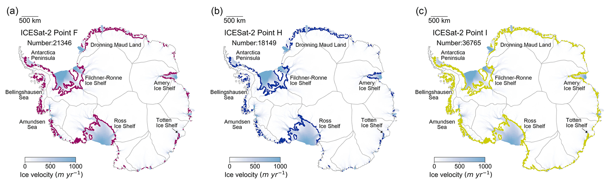
Figure 5 Spatial distributions of ICESat-2-derived grounding zone features of the Antarctic Ice Sheet. (a) ICESat-2-derived inland limits of tidal flexure (Point F; purple dots). (b) ICESat-2-derived inland limit of hydrostatic equilibrium (Point H; blue dots). (c) ICESat-2-derived break in slope (Point I_b; yellow dots). In all subplots, data are superimposed over recent ice velocity magnitudes (Rignot et al., 2017) and IMBIE basin boundary (Shepherd et al., 2018; Rignot et al., 2011b).

Compared with the ICESat-derived GZ product (Brunt et al., 2010a), which has 1497 Point F, 1470 Point H, and 1493 Point I_b locations, the ICESat-2-derived GZ features in this study have greatly improved the GZ density and coverage, including previously poorly mapped regions such as fast-flowing ice streams in the Amundsen Sea embayment. For Points F and H, we obtained near-complete coverage on the Larsen C Ice Shelf, Filchner–Ronne Ice Shelf, Dronning Maud Land, Ross Ice Shelf, and Sulzberger Ice Shelf, including numerous ice rises and ice rumples (Fig. 5a and b). Compared with Points F and H, the ICESat-2-derived Point I_b further improves the GZ coverage (Fig. 5c). It is able to recover the GZ of the fast-flowing glaciers that are difficult to map with the dynamic method, including Pine Island, Thwaites, Kohler, Smith, and Pope glaciers located in the Amundsen Sea embayment as well as the mountainous regions in Victoria Land. In addition, the ICESat-2-derived Point I_b also provides complete coverage for the ice rises and ice rumples across the Antarctic ice shelves, which are not available from the ASAID product (Bindschadler et al., 2011).

3.2 Validation of the inland limit of tidal flexure Point F

3.2.1 Comparison with ICESat-2 crossover measurements

Elevation changes at crossovers on the Filchner–Ronne and Ross ice shelves were mapped in our study (Figs. 6, 7). The transitions from land ice (low $\left|\mathrm{dh}\right|$) to floating ice (high $\left|\mathrm{dh}\right|$) at the crossovers can show the approximate location of the GL (Li et al., 2020), with which we compared our repeat-track-derived GZ results. In general, the crossover-derived GL, where the $\left|\mathrm{dh}\right|$ is 20 cm, which is the minimum detectable tidal range in these two regions, shows good agreement with the ICESat-2-derived Point F (Figs. 6a and 7a).

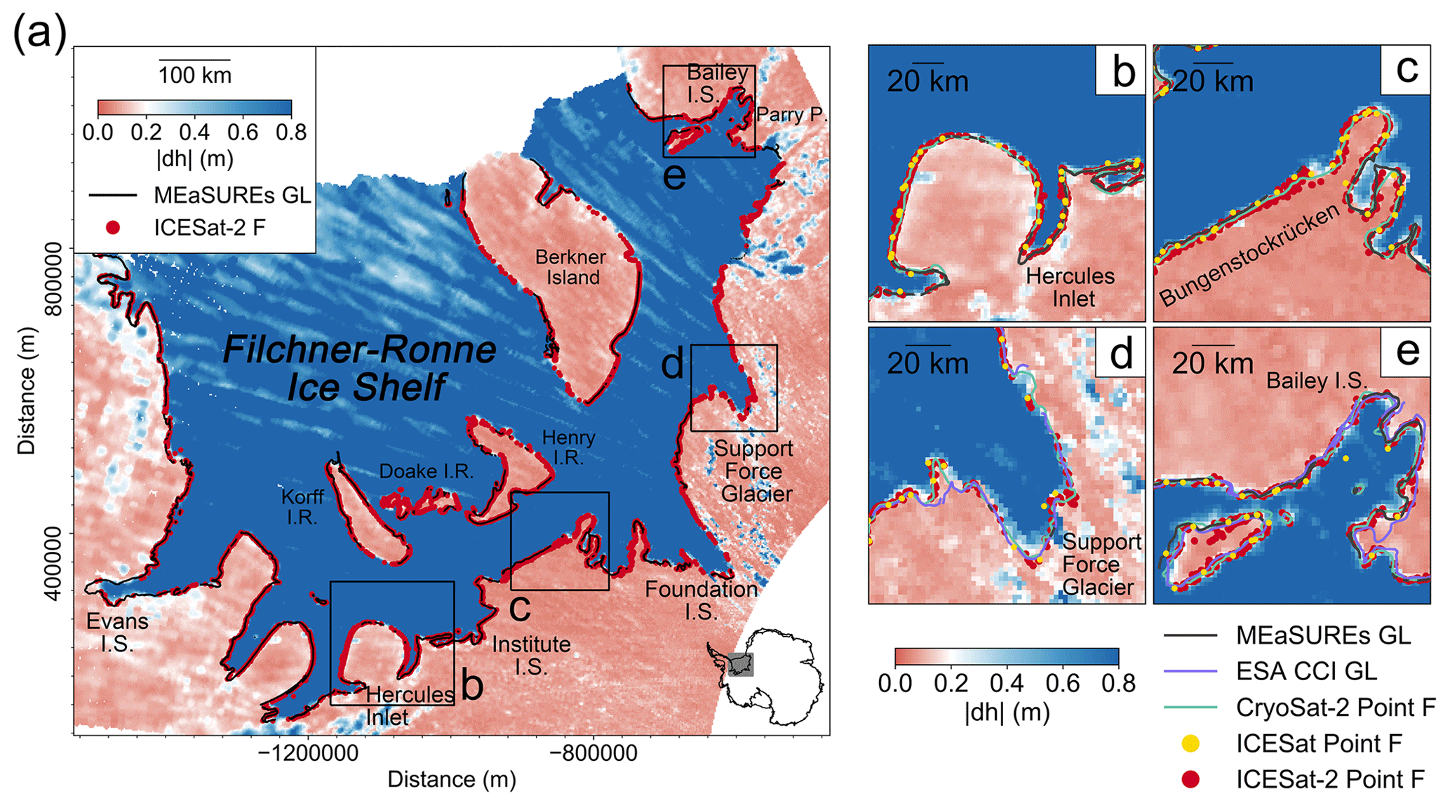
Figure 6 (a) Spatial distribution of the absolute elevation change at ICESat-2 crossovers per 2 km grid cell across the Filchner–Ronne Ice Shelf; the four black boxes denote the individual regions plotted in (b)–(e)​​​​​​​. (b) Hercules Inlet, (c) Bungenstockrücken, (d) Support Force Glacier, (e) Bailey Ice Stream. In subplots (b)–(e), the ICESat-2-derived inland limits of tidal flexure (Point F) are shown as red dots. The ICESat-derived Point F locations are shown as the yellow dots. The MEaSUREs DInSAR-derived Point F (Rignot et al., 2016) is shown as the black line. The ESA CCI DInSAR-derived Point F is shown as the purple line. The CryoSat-2-derived Point F is shown as the green line (Dawson and Bamber, 2020).

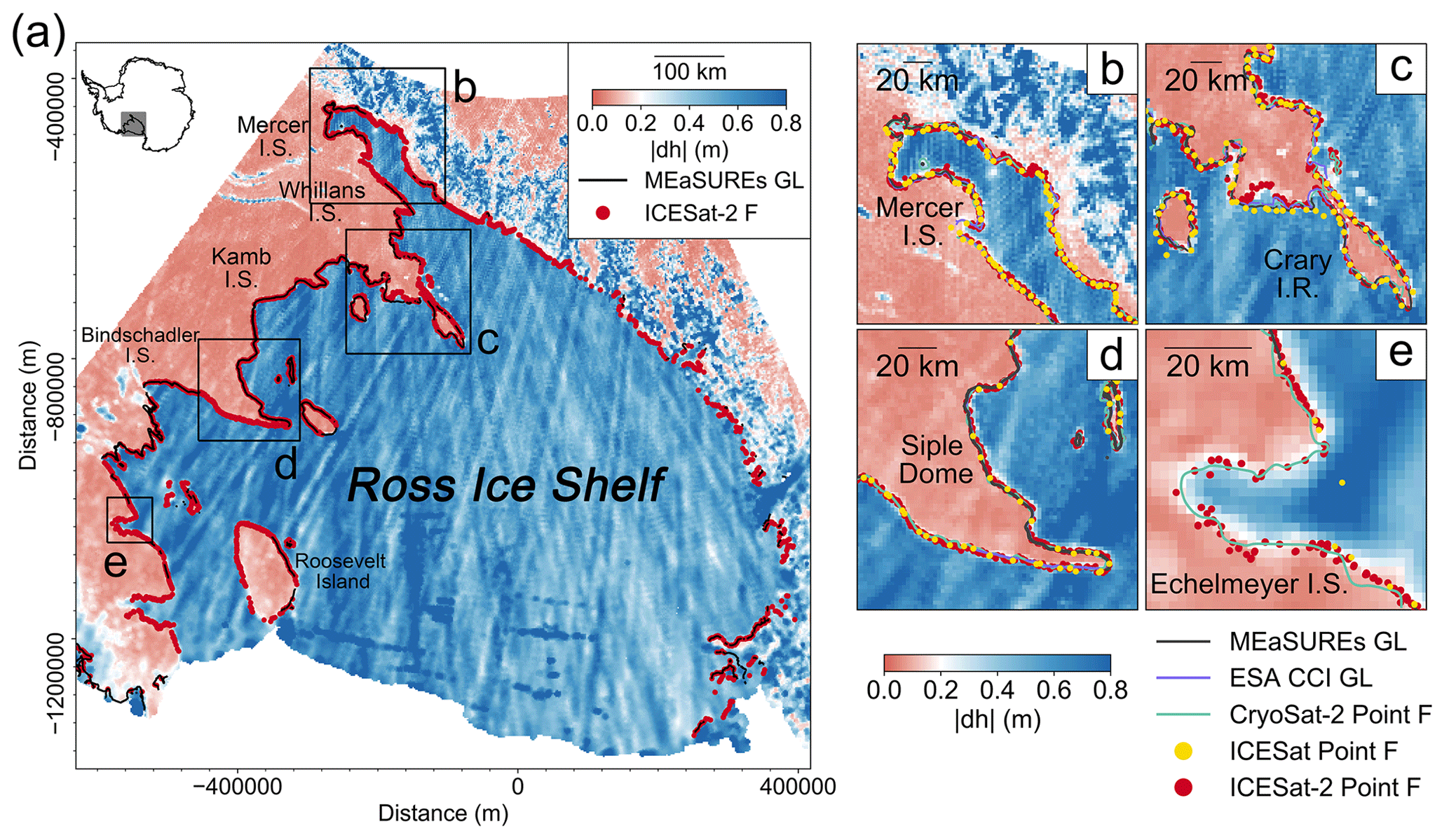
Figure 7 (a) Spatial distribution of the absolute elevation change at ICESat-2 crossovers per 2 km grid cell across the Ross Ice Shelf; the four black boxes denote the individual regions plotted in (b)–(e). (b) Mercer Ice Stream, (c) Crary Ice Rise, (d) Siple Dome, (e) Echelmeyer Ice Stream. In subplots (b)–(e), the ICESat-2-derived inland limits of tidal flexure (Point F) are shown as red dots. The ICESat-derived Point F locations are shown as the yellow dots. The MEaSUREs DInSAR-derived Point F (Rignot et al., 2016) is shown as the black line. The ESA CCI DInSAR-derived Point F is shown as the purple line. The CryoSat-2-derived Point F is shown as the green line (Dawson and Bamber, 2020).

On the main glacier trunk of the Support Force Glacier (Fig. 6d), the crossover-derived GL and ICESat-2-derived Point F align well with the ESA Climate Change Initiative (CCI) DInSAR-mapped Point F in 2016 and the CryoSat-2-derived Point F in 2017. On the western side of the glacier, the ICESat-2-derived Point F, crossover-derived GL, and the CryoSat-2-derived Point F show an approximately 10 km seaward migration compared with the ESA CCI DInSAR-derived Point F in 2016. On the main glacier trunk of Bailey Ice Stream, the crossover-derived GL, ICESat-2-derived Point F, CryoSat-2-derived Point F, MEaSUREs DInSAR-derived Point F, and the ESA CCI DInSAR-derived Point F in 2014 agree well with each other (Fig. 6e). However, on the northern flank of the Parry Peninsula (Fig. 6e), the ESA CCI DInSAR-derived Point F shows an approximately 10 km retreat compared with all the other GL measurements.

On Crary Ice Rise (Fig. 7c), ICESat-2-derived Point F locations agree well with the crossover-derived GL distribution but show a retreat of up to 15 km compared with all the previous GL measurements. On Mercer Ice Stream and Siple Dome, the ICESat-2-derived Point F and crossover-derived GL have good agreement with the previous GL products (Fig. 7b and d). On Echelmeyer Ice Stream, where there is only one ICESat-derived Point F, the ICESat-2-derived Point F locations show an approximately 30 km retreat compared with ICESat-derived Point F but agree well with the CryoSat-2-derived Point F in 2017 and the ICESat-2-crossover-derived GL (Fig. 7e), further confirming the conclusion that ICESat picked the wrong Point F in this region (Dawson and Bamber, 2017).

3.2.2 Comparison with Sentinel-1a/b DInSAR measurements

In addition to comparing the ICESat-2-derived Point F with ICESat-2 crossover measurements and the historic GLs on the Filchner–Ronne and Ross ice shelves, we compared the ICESat-2-derived Point F to the latest pan-Antarctic DInSAR-derived GL product, which was estimated from a deep-learning-based approach by using Sentinel-1a/b synthetic aperture radar (SAR) images in 2018 (Mohajerani et al., 2021). With its acquisition time close to ICESat-2 (up to 1 year apart), we do not expect large separations in GL locations between these two products due to any changes in the GL. The Sentinel-1a/b DInSAR-derived GL has a precision of 200 m (Mohajerani et al., 2021); however due to limitation of Sentinel's coverage in polar regions, this product does not fully cover the Filchner–Ronne and Ross ice shelves. The absolute separations between 2018 DInSAR-derived Point F with ICESat-2-derived Point F are shown in Figs. 8a and A3. Despite the relatively small difference in measurement time, there may still be changes in Point F. In general, the rapid retreat of the grounding line happens in fast ice flow (Konrad et al., 2018). Therefore, we also divided the GL separations into two categories: slow-moving regions where the ice velocity is less than 100 m yr⁻¹ (Fig. 8b) and fast-flowing regions where the ice velocity is higher than 100 m yr⁻¹ (Fig. 8c).

Figure 8 (a) Absolute separations between the ICESat-2-derived landward limit of tidal flexure (Point F) and Sentinel-1a/b DInSAR-derived Point F in 2018 (Mohajerani et al., 2021). (b) Absolute separations in areas where the ice velocity is lower than 100 m yr⁻¹ (Rignot et al., 2017), (c) absolute separations in areas where the ice velocity is higher than 100 m yr⁻¹ (Rignot et al., 2017). In all subplots, data are superimposed over the recent mass change map (Smith et al., 2020b) and IMBIE basin boundary (Shepherd et al., 2018; Rignot et al., 2011b).

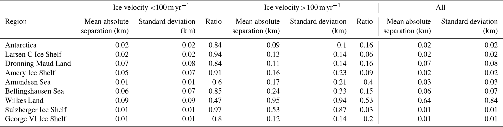
In total, the mean absolute separation and standard deviation across the ice sheet between the two products are 0.02 and 0.02 km, respectively, comparable to the precision of the DInSAR GL product (Table 2). This indicates that the ICESat-2-derived Point F can achieve the same level of precision compared to DInSAR measurements. A total of 84 % of the surveyed GZ is located in slow-moving regions. As expected, the overall mean separations and standard deviations in slow-moving regions, where the GL is normally stable, are lower than in fast-flowing regions. The increase in GL separation in fast-flowing regions between the two products is possibly due to the reduced ICESat-2 GL measurements caused by low signal-to-noise ratio in elevation anomalies of repeat tracks and the fact that DInSAR often suffers from poor signal coherence due to high ice velocity. In the Amundsen Sea embayment and Bellingshausen Sea sector, which have been experiencing substantial mass loss and rapid GL retreat during the past 2 decades (Bamber and Dawson, 2020; Milillo et al., 2017, 2019; Rignot et al., 2014, 2019; Scheuchl et al., 2016), the mean absolute separations in fast-flowing regions are 0.17 and 0.24 km, respectively. The highest mean absolute separation and standard deviation, however, are located in Wilkes Land, East Antarctica (Table 2, Figs. 8a and A3). The Moscow University and Totten Glacier ice shelves in Wilkes Land are both narrow embayments with fast ice flow, where the ice may not be in full hydrostatic equilibrium, and the high ice velocity can often lead to DInSAR measurement errors.

Table 2 Mean absolute separation (km) and standard deviation (km) between ICESat-2-derived landward limit of tidal flexure (Point F) and 2018 DInSAR-derived Point F (Mohajerani et al., 2021) in individual regions.

In slow-moving regions, we observed large deviations between the two products such as the Dronning Maud Land (Figs. 8b and 9a). They are possibly caused by the ephemeral grounding of ice on the scale of kilometres across the ice plain with low surface slope as the ocean tide rises and falls (Bindschadler et al., 2011; Brunt et al., 2011; Milillo et al., 2017). Here we took two examples to demonstrate the short-term GZ feature migration induced by ocean tide oscillation. On the Novyy Island of Dronning Maud Land, the distance between the ICESat-2-derived Point F along the right beam of track 145 is about 2 km compared with the 2018 DInSAR-derived Point F (Mohajerani et al., 2021) (Fig. 9a), while the ICESat-2-derived Point F along the left beam of track 153 in the same region is less than 100 m away from the DInSAR-derived Point F (Fig. 9f). The large difference in Point F location is not caused by errors in methodology but is due to the tidal variations on a lightly grounded ice plain in this region. The tidal range at Point F along track 145 is 0.41 m, while it is 1.03 m at Point F along track 153. The observation suggests that the ice shelf is grounded at low tide and floating at high tide (Brunt et al., 2011).

Figure 9 Comparison between the inland limit of tidal flexure (Point F) from repeat-track analysis for two tracks located in the same region on the Dronning Maud Land under different ocean tidal amplitude ranges. Same as Fig. 3, (a)–e) show ICESat-2 repeat-track analysis for three right beams from repeat cycles 6, 7, and 8 in beam pair 2 of track 145. (f–j) ICESat-2 repeat-track analysis for three left beams from repeat cycles 3, 7, and 8 in beam pair 3 of track 153.

3.3 Validation of the break in slope Point I_b

3.3.1 Comparison with ICESat-2 crossover measurements

Although Point F and Point I_b are two different GZ features derived from different techniques, these two features should be close in location (apart from where there is the presence of an ice plain) (Brunt et al., 2011; Christie et al., 2016). To validate the ICESat-2-derived Point I_b, we first compared them with the crossover-derived GL from ICESat-2 ascending and descending tracks at the Filchner–Ronne and Ross ice shelves (Figs. A1 and A2). Similar to ICESat-2-derived Point F, the ICESat-2-derived Point I_b shows good agreement with the crossover-derived GL in these two regions. In addition, the ICESat-2-derived Point I_b and crossover-derived GL are able to capture the complex inlets, such as the eastern flank of Hercules Inlet of Filchner–Ronne Ice Shelf (Fig. A1b) and the Mercer Ice Stream of Ross Ice Shelf (Fig. A2b), where ASAID Point I_b failed to do so. On Bungenstockrücken of Filchner–Ronne Ice Shelf, there exists an approximately 3 km deviation between the ICESat-2-derived Point I_b and the crossover-derived GL (Fig. A1c). This directly confirms the existence of an ice plain, which is defined as grounded ice with low surface slope adjacent to the GL and where the Point I_b is several kilometres landward of Point F (Brunt et al., 2011). In comparison, the ephemeral grounding of ICESat-2-derived Point F shown in Fig. 6c is likely to be caused by tidal variations inside this ice plain (Brunt et al., 2011).

3.3.2 Comparison with the ASAID product and Sentinel-1a/b DInSAR measurements

We also compared the ICESat-2-derived Point I_b directly with the break in slope from the ASAID product (Figs. 10 and A4, Table 3), which was delineated from Landsat-7 optical images obtained during 1999 and 2003 based on image brightness, also called shape from shading (Bindschadler et al., 2011). The positional accuracies of ASAID Point I_b range from ±52 m for land and ocean terminating to ±502 m for outlet glaciers (Bindschadler et al., 2011). The mean absolute separation and standard deviation for the whole Antarctic Ice Sheet between ICESat-2-derived Point I_b and ASAID Point I_b are 0.43 and 0.43 km, respectively (Table 3). On Larsen C Ice Shelf, the mean absolute separation and standard deviation are lowest, which are 0.19 and 0.17 km, respectively. Larsen C Ice Shelf in general is a slow-moving mountainous region, and the ASAID Point I_b is a good representation of the grounding line (Li et al., 2020). In similar regions with slow ice flow and steep surface gradients such as Sulzberger Ice Shelf and George VI Ice Shelf, the GL separations are also small (Table 3, Fig. A4). The highest separations are located in the fast-flowing regions of the Amundsen Sea embayment; the mean absolute separation and standard deviation are 1.42 and 1.23 km, respectively. For comparison, we also calculated the separations between the ICESat-2-derived Point I_b and the DInSAR-derived Point F in 2018 (Figs. 11 and A5, Table 4). The mean absolute separation and standard deviation between ICESat-2-derived Point I_b and DInSAR-derived Point F in 2018 over the Antarctic Ice Sheet are 0.02 and 0.02 km (Table 4), respectively, which are of the same magnitudes as the ICESat-2-derived Point F. Over the fast-flowing ice streams of the Amundsen Sea embayment, the mean absolute separation and standard deviation are 0.04 and 0.04 km, respectively, much lower than the ASAID Point I_b.

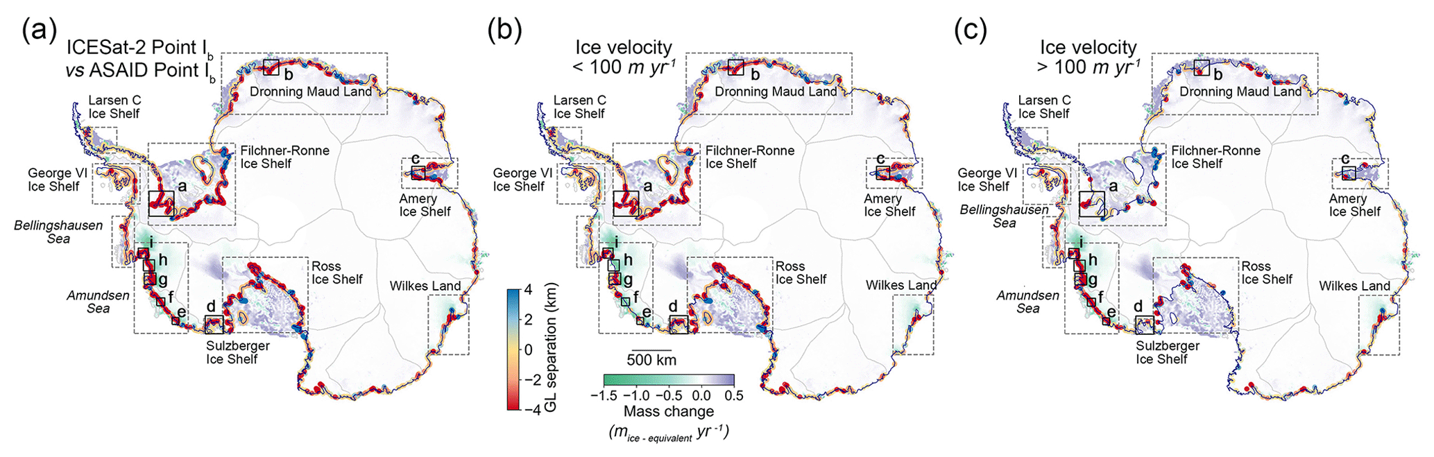
Figure 10 (a) Separations between the ASAID-derived break in slope and ICESat-2-derived break in slope (negative value is retreating while positive value is advancing). (b) Regions with ice velocity (Rignot et al., 2017) less than 100 m yr⁻¹, (c) regions with ice velocity larger than 100 m yr⁻¹. The black boxes denote the spatial extents of regions mapped in Fig. 12. In all subplots, data are superimposed over the recent mass change map (Smith et al., 2020b) and IMBIE basin boundary (Shepherd et al., 2018; Rignot et al., 2011b).

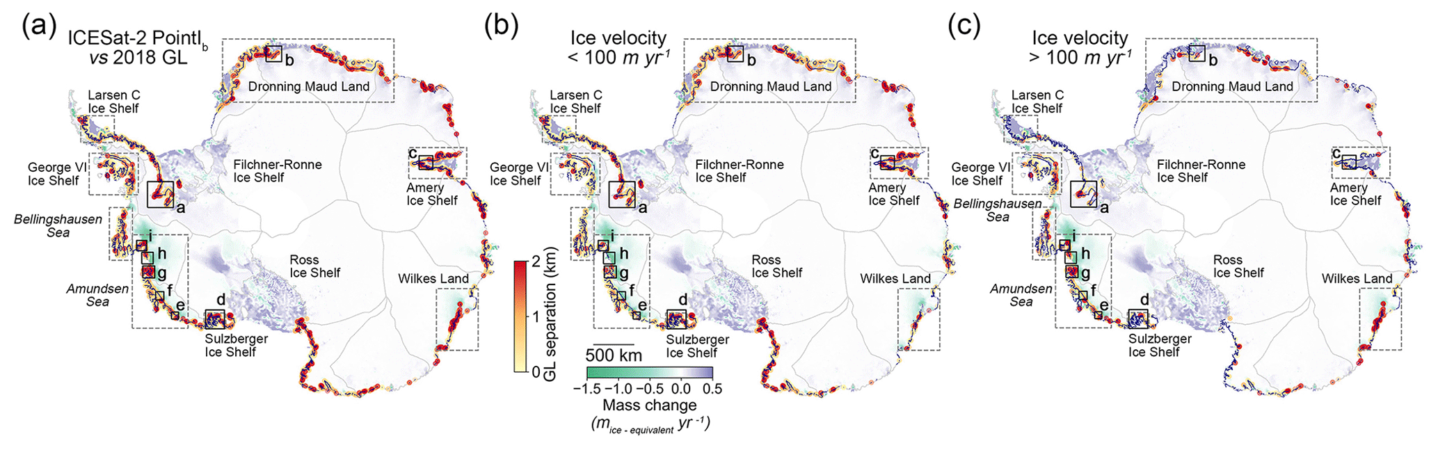
Figure 11 (a) Absolute separations between the ICESat-2-derived break in slope (Point I_b) and 2018 DInSAR-derived Point F (Mohajerani et al., 2021). (b) Regions with ice velocity (Rignot et al., 2017) less than 100 m yr⁻¹, (c) regions with ice velocity larger than 100 m yr⁻¹. The black boxes denote the spatial extents of regions mapped in Fig. 12. In all subplots, data are superimposed over the recent mass change map (Smith et al., 2020b) and IMBIE basin boundary (Shepherd et al., 2018; Rignot et al., 2011b).

Table 3 Mean absolute separation (km) and standard deviation (km) between ICESat-2-derived break in slope (Point I_b) and ASAID break-in-slope product (Bindschadler et al., 2011) in individual regions.

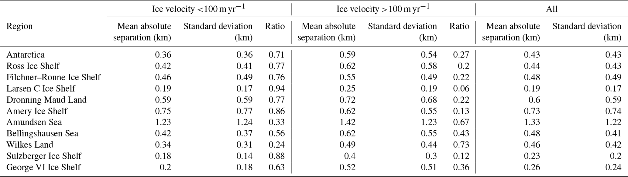
Table 4 Mean absolute separation (km) and standard deviation (km) between ICESat-2-derived break in slope (Point I_b) and 2018 DInSAR-derived Point F (Mohajerani et al., 2021) in individual regions.

Detailed spatial distribution maps of the ICESat-2-derived Point I_b, as well as four other GZ products, including the DInSAR-derived Point F in 2017 for Thwaites Glacier (Milillo et al., 2019), the DInSAR-derived Point F in 2018 (Mohajerani et al., 2021), the ASAID Point I_b during 1999 and 2003 (Bindschadler et al., 2011), and the ICESat-derived Point I_b (Brunt et al., 2010a), are shown in Fig. 12. In mountainous regions with a stable GL, such as the Sulzberger Ice Shelf (Fig. 12d), different GZ products match well with each other. On fast-flowing glaciers where the subglacial bed and surface slopes are shallow, Point I_b is difficult to identify from satellite imagery based on a change in image brightness (Bindschadler et al., 2011; Christie et al., 2016, 2018). This is evident on the Pope and Smith glaciers (Fig. 12g), where Point I_b from the ASAID product cannot identify the correct ice sheet boundary. In addition, on the fast-flowing Jutulstraumen Glacier (ice velocity >700 m yr⁻¹) at Dronning Maud Land (Fig. 12b), there exists a deviation of up to 15 km between the ICESat-2-derived Point I_b and ASAID Point I_b. In contrast, in regions which have been experiencing ice dynamical thinning and rapid grounding line retreats along the Amundsen Sea embayment (Chuter et al., 2017; Smith et al., 2020b​​​​​​​; Bamber and Dawson, 2020), the ICESat-2-derived Point I_b has good agreement with the latest DInSAR-derived Point F in 2018 (Fig. 12e–i). Moreover, they both show a pervasive retreat compared with the ASAID Point I_b identified between 1999 and 2003, especially on the fast-flowing glaciers of sustained GL retreat, such as the Berry Glacier in Fig. 12e; the unnamed glaciers along Getz Ice Shelf in Fig. 12f; the Pope, Smith, and Kohler glaciers in Fig. 12g; the Thwaites Glacier in Fig. 12h; and the Pine Island Glacier in Fig. 12i. In the “butterfly” region of Thwaites Glacier, which is featured by rapid ice thinning and grounding line retreat during the past 2 decades (Milillo et al., 2019), there is an almost 10 km landward migration between the ASAID Point I_b and the ICESat-2-derived Point I_b (Fig. 4g). Similar to Thwaites Glacier, Getz Ice Shelf has also been experiencing ice dynamical thinning (Selley et al., 2021) and GL retreat (Christie et al., 2018; Konrad et al., 2018). The ICESat-2-derived Point I_b at an unnamed fast-flowing glacier shows an approximately 6 km landward migration compared with the ASAID break in slope (Fig. 4m).

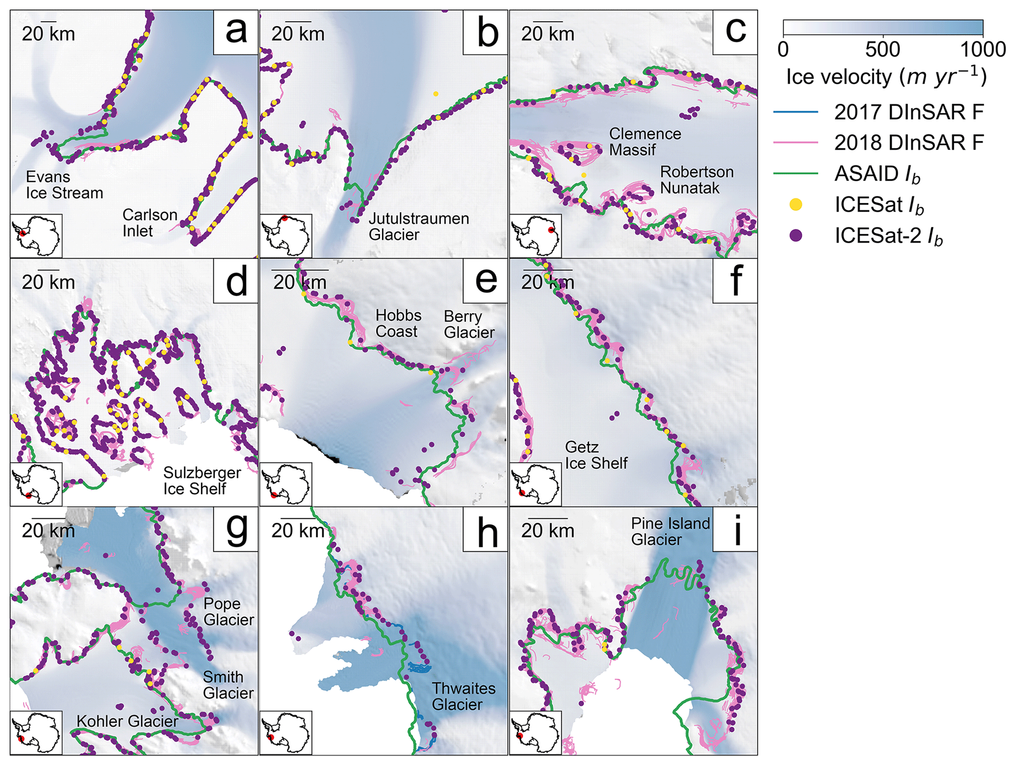
Figure 12 Spatial distributions of ICESat-2-derived break in slope (Point I_b) in each individual region (black boxes in Figs. 10 and 11). For comparison, ICESat-derived Point I_b locations are shown as the yellow dots (Brunt et al., 2010a), ASAID-derived Point I_b is shown as the green line (Bindschadler et al., 2011), DInSAR-derived Point F in 2018 is shown as the pink line (Mohajerani et al., 2021), and DInSAR-derived Point F in 2017 on Thwaites Glacier (panel h) is shown as the blue line (Milillo et al., 2019). In all subplots, data are superimposed over recent ice surface velocity magnitudes (Rignot et al., 2017) in Antarctica polar stereographic projection (EPSG:3031).

3.4 Validation of the inshore limit of hydrostatic equilibrium Point H

The inshore limit of hydrostatic equilibrium, mapped from the ASAID project, is the most complete product for Point H to date and was derived from ICESat-derived Point H and Landsat-7 imagery (Bindschadler et al., 2011). The positional error in Point H from the ASAID product is about 2 km. The absolute separation between the ICESat-2-derived Point H and ASAID Point H is shown in Fig. 13. The overall mean absolute separation and standard deviation for the whole Antarctic Ice Sheet between the two products are 1.65 and 1.29 km (Table 5), respectively, which are within the 2 km geolocation error in ASAID Point H. However, they vary by region (Fig. 13 and Table 5). The Larsen C Ice Shelf has the smallest mean absolute separation and standard deviation, while the Amery Ice Shelf has the highest mean absolute separation and standard deviation of 2 and 1.62 km, respectively.

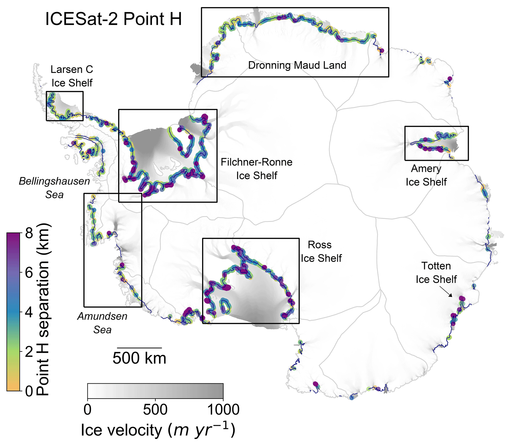
Figure 13 The absolute separations between the ICESat-2-derived Point H and the Point H from the ASAID grounding line project (Bindschadler et al., 2011). Data are superimposed over recent ice surface velocity magnitudes (Rignot et al., 2017) and the IMBIE basin boundary (Shepherd et al., 2018; Rignot et al., 2011b) in Antarctic polar stereographic projection (EPSG:3031).

Table 5 The mean absolute separation and standard deviations between ICESat-2-derived Point H and ASAID-derived Point H (Bindschadler et al., 2011).

The location of Point H is not stagnant but changes with ocean tides. On the western flank of the Skytrain Ice Rise on the Filchner–Ronne Ice Shelf (Fig. 14), the ICESat-2-derived Point F locations along the left (Fig. 14a–e) and right beams (Fig. 14f–j) of track 1071 are separated by 158 m. However, the distance between the ICESat-2-derived Point H locations is 6 km. The tidal range at the seaward Point H along the left beam of track 1071 is 3.3 m, while it is only 0.8 m at the landward Point H along the right beam of track 1071. This indicates that the ocean tide oscillation will not only influence the grounding point of the ice but will also change the point of hydrostatic equilibrium. More examples will be used to fully investigate the influence of ocean tides on the GZ width in future research.

Figure 14 Comparison between the inshore limit of hydrostatic equilibrium (Point H) from repeat-track analysis for left and right beams of track 1071 located on the Skytrain Ice Rise under different ocean tidal amplitude ranges. Same as Fig. 3, (a)–e) show ICESat-2 repeat-track analysis for three left beams from repeat cycles 3, 5, and 7 in beam pair 3 of track 1071. (f–j) ICESat-2 repeat-track analysis for three right beams from repeat cycles 5, 6, and 7 in beam pair 3 of track 1071.

4 Discussion

Although good agreement exists between the ICESat-2-derived Point F and DInSAR-derived Point F in 2018, large deviations have been observed in slow-moving regions due to short-term GL migrations over ice plains caused by ocean tides. The DInSAR-derived Point F using Sentinel-1a/b interferograms in 2018 sampled different GL positions with changes in ocean tides; however, it fails to capture the ephemeral grounding observed in this study (Fig. 9). This indicates that 1 year's worth of DInSAR data may not be fully adequate to address the migration of GL in different ocean tide amplitudes within a tidal cycle (Mohajerani et al., 2018).

By comparing the ICESat-2-derived Point F with ICESat-2 crossovers, as well as with several published GZ products on the Filchner–Ronne and Ross ice shelves, we are able to detect possible errors in different GZ products. The large landward deviations in the ESA CCI DInSAR-derived Point F on the western flank of Support Force Glacier in 2016 and the northern flank of Parry Peninsula in 2014, compared with all the other GZ products, indicate that the ESA CCI DInSAR-derived Point F locations are likely to be in error. A landward GL migration of up to 15 km was identified for ICESat-2-derived Point F at Crary Ice Rise compared with previous GL products, which is coincident with high mass loss in this region (Smith et al., 2020b), indicating that it can be a possible region of GL retreat. Further research is needed to fully understand the reason why the GL has been retreating in this region.

In highly crevassed and fast-flowing glaciers with low tidal amplitudes (Padman et al., 2002), such as Pine Island Glacier and Thwaites Glacier located in the Amundsen Sea embayment, it is difficult to capture both Points F and H based on the dynamic method, which samples elevation changes at different tidal phases using repeat-track analysis. The fast movement of the glaciers can cause extensive advection of ice surface features on the floating ice, such as crevasses and surface undulations (Moholdt et al., 2014; Khazendar et al., 2013). This will result in high elevation anomalies not associated with ocean tides, making it difficult to identify the limit of ice flexure. A Lagrangian framework has been used to reduce the elevation change anomalies caused by feature advection (Moholdt et al., 2014; Dutrieux et al., 2013). This method, however, requires the movement of ice features synchronized with the ice flow, which is only applicable on floating ice shelves (Marsh et al., 2016). Thus it is not suitable for this study as we are only interested in the transition between grounded ice and floating ice. Unlike the limit of tidal flexure Points F and H that directly depend on the tidal variations, the break-in-slope point is the location where the ice “feels” the bed sufficiently to react to the stresses associated with this contact, and it is not influenced by the temporal tidal variations (Bindschadler et al., 2011). Also the elevation differences measured by Points F and H are always noisier than the absolute surface elevation measured by Point I_b. The static method developed in this study is able to reliably detect the break in slope even in highly crevassed fast-flowing glaciers, such as Thwaites Glacier and Getz Ice Shelf, where the break in slope is less prominent, and the optical imagery approaches are normally unable to interpret the correct break in slope (Bindschadler et al., 2011; Rignot et al., 2011a).

Compared with the ASAID break-in-slope delineation from Landsat-7 images, ICESat-2-derived Point I_b and the latest DInSAR-derived Point F in 2018 both show large landward deviations in the Amundsen Sea embayment. These landward deviations can possibly be attributed to the GL retreat, given the fact that dynamical mass loss has been taking place in this region (Smith et al., 2020b). However, as the ICESat-2-derived Point I_b and ASAID Point I_b are calculated based on two different methods, there will always be differences between these two boundaries due to data quality or incorrect interpretation (Bindschadler et al., 2011); therefore caution is needed when identifying the true GL retreat. The Antarctic GZ product produced in this study uses only 18 months of ICESat-2 ATL06 datasets; with more repeat cycles available in future, we will be able to map the GZ over the same region repeatedly and efficiently using the same techniques. This could reduce the errors in interpreting GL migrations.

5 Data availability

The​​​​​​​ dataset produced in this study is available at the University of Bristol data repository, data.bris, at https://doi.org/10.5523/bris.bnqqyngt89eo26qk8keckglww (Li et al., 2021). It is also archived and maintained at the National Snow and Ice Data Center (NSIDC). The ICESat-2 data used in this study are available from the NSIDC (https://doi.org/10.5067/ATLAS/ATL06.003, Smith et al., 2020a).​​​​​​​

6 Summary and conclusion

We present the first ICESat-2-derived high-resolution Antarctic GZ product using 18 months of data, including three GZ features (Li et al., 2021). This product has been derived using automated techniques developed in this study based on ICESat-2 repeat tracks and has been validated using a crossover analysis of ICESat-2 data over the Filchner–Ronne and Ross ice shelves and against the recent DInSAR measurements. A total of 21 346 Point F (the landward limit of ice flexure), 18 149 Point H (the inshore limit of hydrostatic equilibrium), and 36 765 Point I_b (the break in slope) locations were identified for the Antarctic Ice Sheet. This represents a significant increase in GZ density compared with ICESat measurements. The mean absolute separation and standard deviation between the ICESat-2-derived Point F and the DInSAR-derived GL product in 2018 are 0.02 and 0.02 km, respectively, comparable to the precision of the DInSAR product. While the dynamic method can have difficulties defining the GZ in highly crevassed fast-flowing glaciers with low tidal range, such as the fast-flowing glaciers in the Amundsen Sea embayment, the static method is able to retrieve the break in slope reliably in these regions. The mean absolute separation and standard deviation between the ICESat-2-derived Point I_b and the DInSAR-derived Point F in 2018 over the fast-flowing regions in the Amundsen Sea embayment are 0.04 and 0.04 km, respectively. Additionally, both ICESat-2-derived Point I_b and the DInSAR-derived Point F show pervasive landward migrations compared with the ASAID product. This coincides with the contemporaneous mass loss and GL retreat in this region.

Although our study period only covers 18 months, we are able to detect short-term GZ migration due to ocean tidal oscillation. Examples of repeat-track analysis in Dronning Maud Land and the Filchner–Ronne Ice Shelf show that the influence of ocean tide variations will not only change the grounding location of the ice but will also influence the point of full hydrostatic equilibrium for the floating ice. A more detailed analysis of the relationship between ocean tide variations, GZ width, and different geophysical factors is needed in the future. With more repeat cycles coming out in the next few years, we will be able to map the GZ features based on the same techniques developed in this study repeatedly and efficiently. This will allow for tracking GL migration at higher accuracy and provide more comprehensive insights into ice sheet instability, which is valuable for both the cryosphere and sea level science communities.

Appendix A

Figure A1 (a) Spatial distribution of the absolute elevation change at ICESat-2 crossovers per 2 km grid cell across the Filchner–Ronne Ice Shelf overlaid with ICESat-2-derived break in slope (Point I_b); the four black boxes denote the individual regions plotted in (b)–(e). (b) Hercules Inlet, (c) Bungenstockrücken, (d) Foundation Ice Stream, (e) Bailey Ice Stream. In all subplots, the ICESat-2-derived breaks in slope (Point I_b) are shown as red dots. The ICESat-derived Point I_b locations are shown as the yellow dots. The ASAID Point I_b is shown as the black line (Bindschadler et al., 2011).

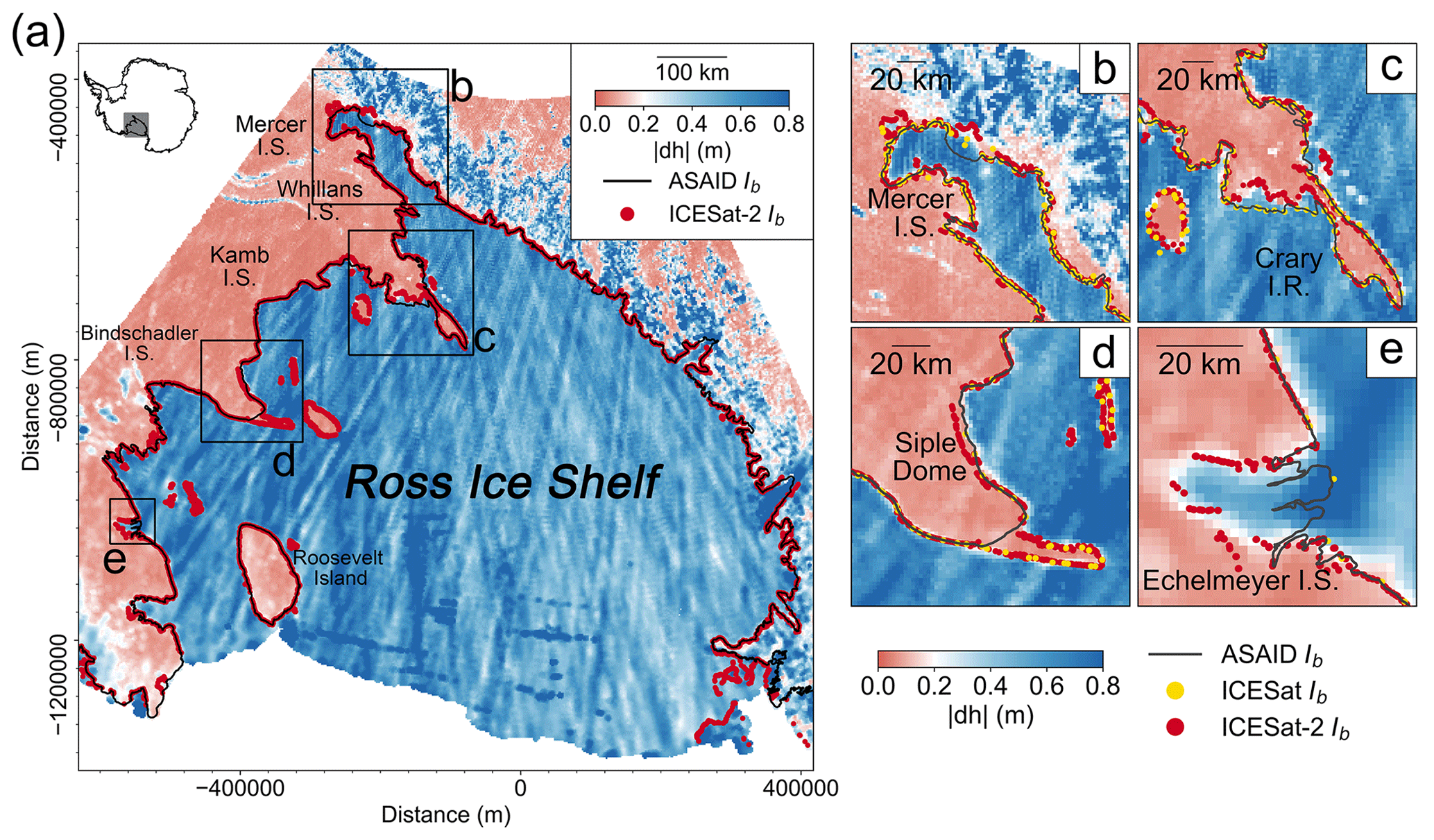
Figure A2 (a) Spatial distribution of the absolute elevation change at ICESat-2 crossovers per 2 km grid cell across the Ross Ice Shelf overlaid with ICESat-2-derived break in slope (Point I_b); the four black boxes denote the individual regions plotted in (b)–(e). (b) Mercer Ice Stream, (c) Crary Ice Rise, (d) Siple Dome, (e) Echelmeyer Ice Stream. In all subplots, the ICESat-2-derived breaks in slope (Point I_b) are shown as red dots. The ICESat-derived Point I_b locations are shown as the yellow dots. The ASAID Point I_b is shown as the black line (Bindschadler et al., 2011).

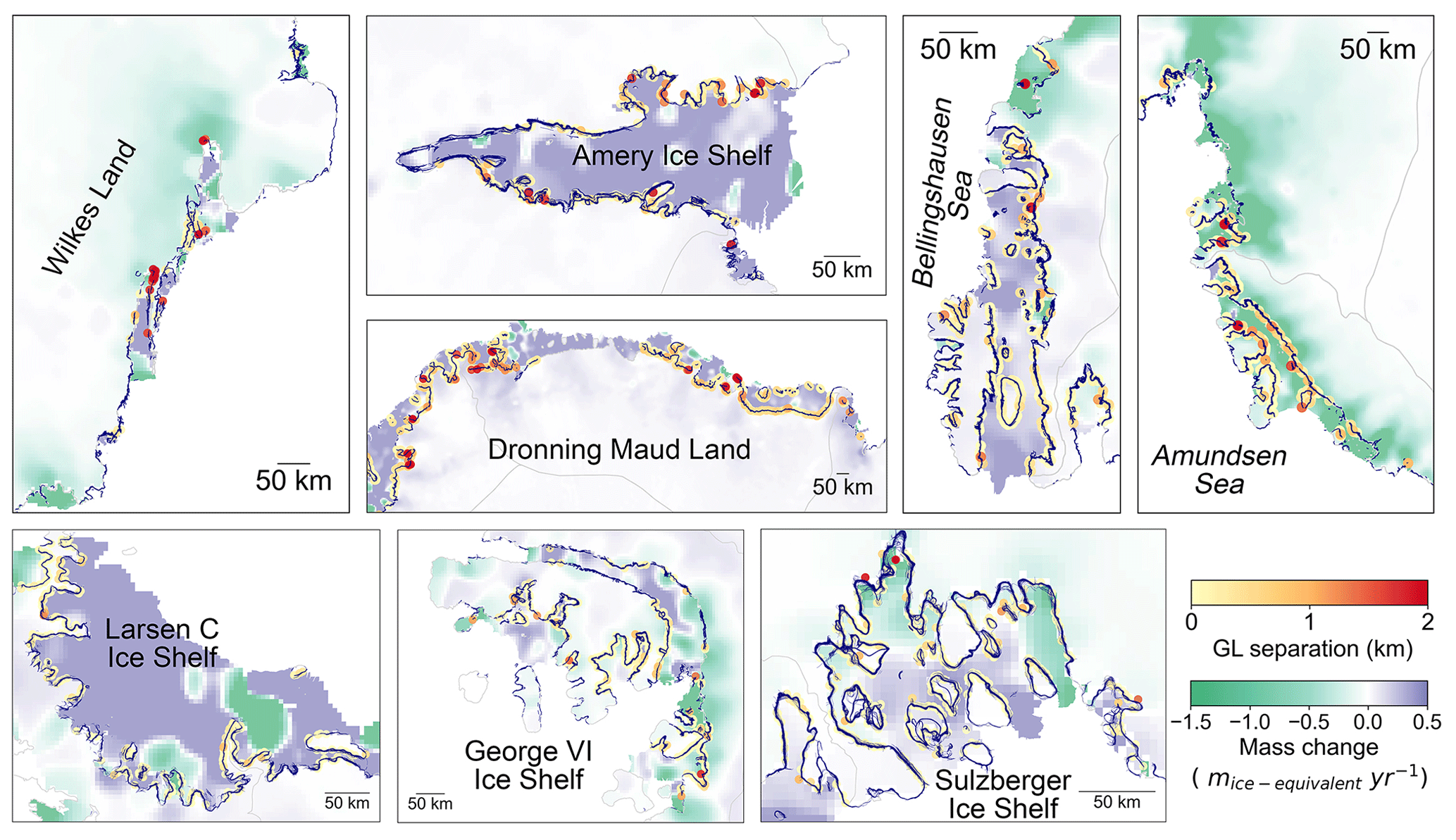
Figure A3 Spatial distributions of the absolute separations between the ICESat-2-derived landward limit of tidal flexure (Point F) and Sentinel-1a/b DInSAR-derived Point F in 2018 of individual regions in Table 2; the spatial extents of each region are shown as black boxes in Fig. 8. In all subplots, data are superimposed over the recent mass change map (Smith et al., 2020b); the blue line is the Sentinel-1a/b DInSAR-derived Point F in 2018 (Mohajerani et al., 2021), and the light-grey line is the IMBIE basin boundary (Shepherd et al., 2018; Rignot et al., 2011b).

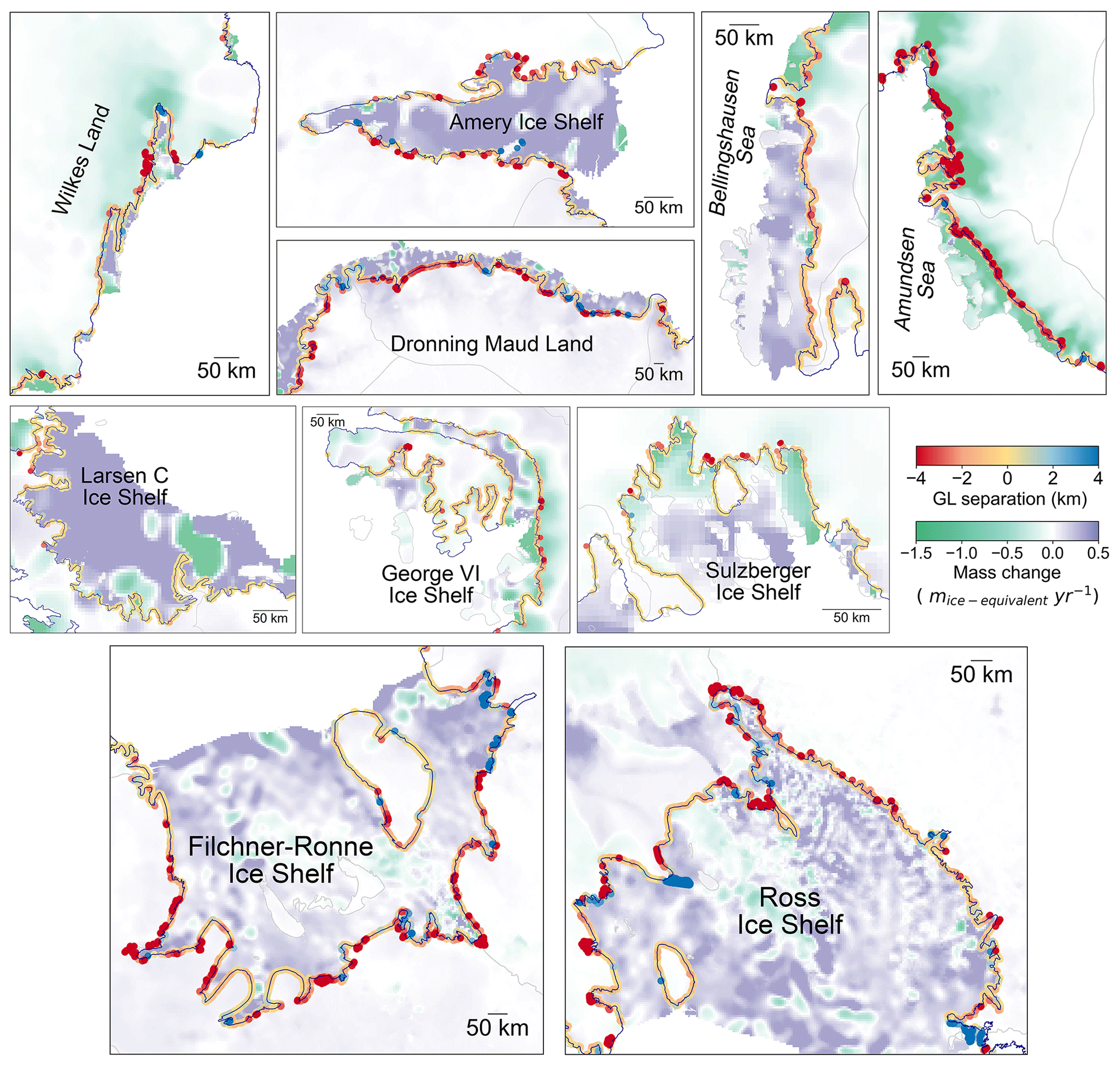
Figure A4 Spatial distributions of the separations between the ASAID-derived break in slope and ICESat-2-derived break in slope (Point I_b) (the negative value is retreating, while the positive value is advancing) in individual regions in Table 3; the spatial extents of each region are shown as dashed grey boxes in Fig. 10. In all subplots, data are superimposed over the recent mass change map (Smith et al., 2020b); the black line is the ASAID-derived break in slope (Bindschadler et al., 2011), and the light-grey line is the IMBIE basin boundary (Shepherd et al., 2018; Rignot et al., 2011b).

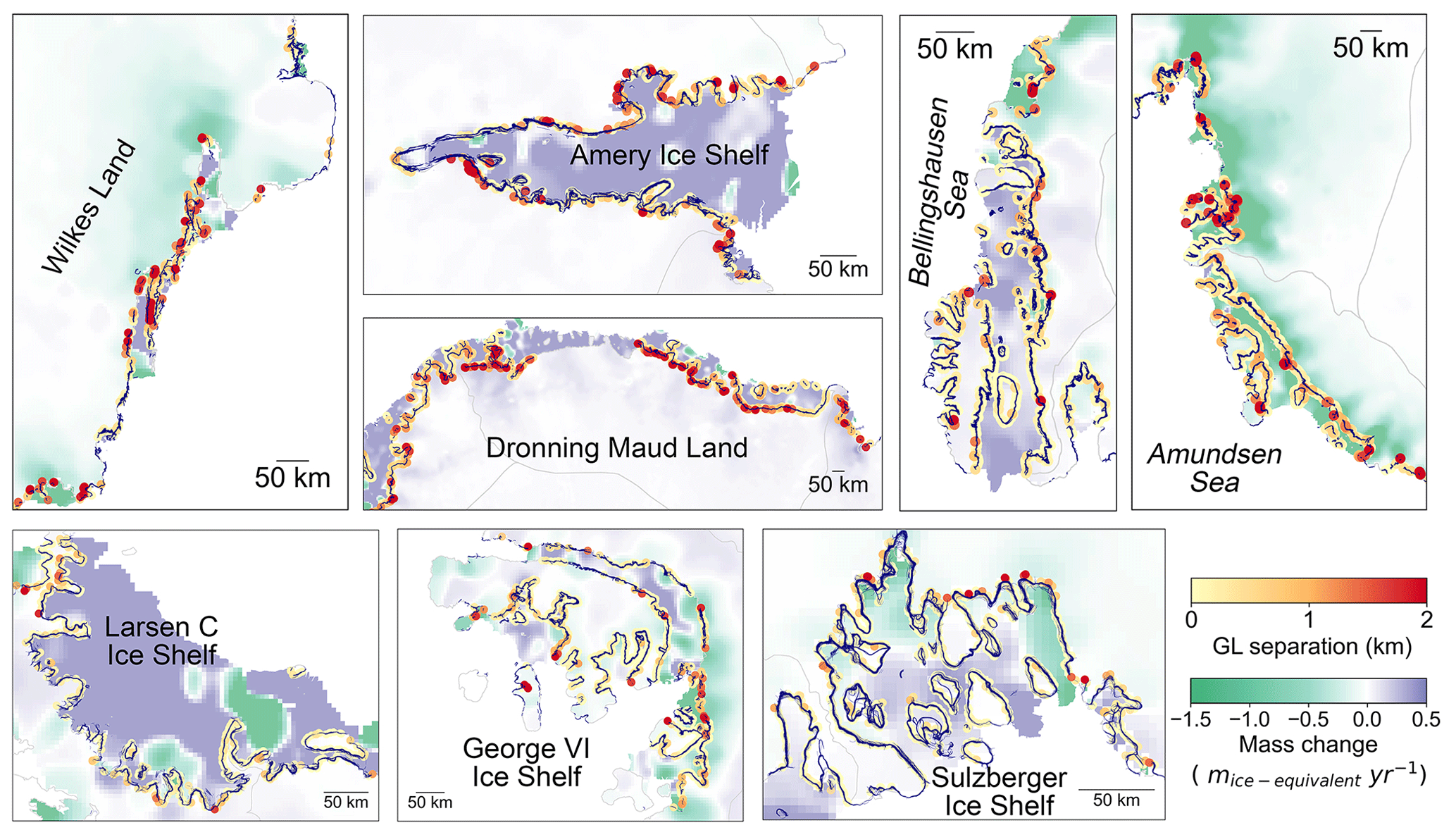
Figure A5 Spatial distributions of the absolute separations between the ICESat-2-derived break in slope (Point I_b) and Sentinel-1a/b DInSAR-derived Point F in 2018 of individual regions in Table 4; the spatial extents of each region are shown as dashed grey boxes in Fig. 11. In all subplots, data are superimposed over the recent mass change map (Smith et al., 2020b); the blue line is the Sentinel-1a/b DInSAR-derived Point F in 2018 (Mohajerani et al., 2021), and the light-grey line is the IMBIE basin boundary (Shepherd et al., 2018; Rignot et al., 2011b).

Table A1 List of different grounding line (GL) products used to update the Depoorter et al. (2013) grounding line for the composite grounding line generated in Sect. 2.2.