Long-term ash dispersal dataset of the Sakurajima Taisho eruption for ashfall disaster countermeasure

A large volcanic eruption can generate large amounts of ash which affect the socio-economic activities of surrounding areas, affecting airline transportation, socio-economics activities, and human health. Accumulated ashfall has devastating impacts on areas surrounding the volcano and in other regions, and eruption scale and weather conditions may escalate ashfall hazards to wider areas. It is crucial to discover places with a high probability of exposure to ashfall deposition. Here, as a reference for ashfall disaster countermeasures, we present a dataset containing the estimated distributions of the ashfall deposit and airborne ash concentration, obtained from a simulation of ash dispersal following a large-scale explosive volcanic eruption. We selected the Taisho (1914) eruption of the Sakurajima volcano, as our case study. This was the strongest eruption in Japan in the last century, and our study provides a baseline for a worst-case scenario. We employed one eruption scenario (OES) approach by replicating the actual event under various extended weather conditions to show how it would affect contemporary Japan. We generated an ash dispersal dataset by simulating the ash transport of the Taisho eruption scenario using a volcanic ash dispersal model and meteorological reanalysis data for 64 years (1958–2021). We explain the dataset production and provide the dataset in multiple formats for broader audiences. We examine the validity of the dataset, its limitations, and its uncertainties. Countermeasure strategies can be derived from this dataset to reduce ashfall risk. The dataset is available at the DesignSafe-CI Data Depot: https://www.designsafe-ci.org/data/browser/public/designsafe.storage.published/PRJ-2848v2 or through the following DOI: https://doi.org/10.17603/ds2-vw5f-t920 by selecting Version 2 (Rahadianto and Tatano, 2020).

1 Introduction

A volcanic eruption emits dangerous pollutants including tephra in the form of very fine ash. These affect human lives over vast areas (Bonadonna et al., 2021).

When a large volcanic eruption occurs, volcanic ashes can travel far from the volcano source, disrupting socio-economic activities in many ways. Fast-travelling ash endangers a larger population and significantly disrupts airline transportation (Folch et al., 2012; Peng and Peterson, 2012; Tanaka and Iguchi, 2019). Settled volcanic ash (i.e. ashfall) directly affects human health and livelihoods, destroys vegetation, crops, and pastures, and physically damages infrastructure by clogging drainage systems, contaminating water supplies, disrupting traffic, and damaging vehicles on roads (Barsotti et al., 2010; Ayris and Delmelle, 2012; Wilson et al., 2012; Damby et al., 2013; Poulidis et al., 2018). The cumulative weight of ashfall on the roof can collapse buildings and short circuit electricity inside them (Zuccaro et al., 2013; Hampton et al., 2015). Evidence from large eruption events (e.g. St. Helens in 1980, Mt. Pinatubo in 1991, Eyjafjallajökull in 2010) demonstrates the cataclysmic consequences of ashfall in wide areas (Tilling et al., 1990; Fero et al., 2008, 2009; Folch et al., 2012; Peng and Peterson, 2012). Ashfall hazards are uncertain and depend on the eruption magnitude and intensity and the wind condition at the time of eruption. Because socio-economic activities have dynamically changing exposures to ashfall hazards, we believe that estimating the risk of finding effective countermeasures is critical.

Currently, densely populated and modernised cities require volcanic risk reduction strategies (Miyaji et al., 2011) to lessen the impacts of ashfall. Assessing the risks to infrastructure, human lives, and economic systems allows better response plans to be developed. Hazard and risk assessment for ashfall mostly relies on quantifying accumulated ashfall on the ground, then extending the analysis by combining appropriate social data (e.g. population or building data, or others). Many researchers used this approach to determine the probability of impacts of future eruption events (Jenkins et al., 2014, 2015, 2018; Wilson et al., 2012; Biass et al., 2017). An ashfall risk assessment requires long-term weather data for statistical analysis and simulations of typical and exceptional conditions (Hattori et al., 2013, 2016). Long-term ashfall deposit data encompassing vast impact areas during an extended period is an important requisite for conducting such a study. This paper presents a generated dataset of ash dispersal over a vast region of Japan for 64 years (1958–2021). Using the Taisho eruption of the Sakurajima volcano, the largest and the strongest eruption in Japan during the last century (Todde et al., 2017; Poulidis et al., 2018) as a case study, we simulated a volcanic ash transport and dispersion model (VATDM) to demonstrate an ash dispersal process over entire Japan. We adapt an OES (one eruption scenario) strategy as a baseline for a worst-case scenario (Bonadonna, 2006; Barsotti et al., 2018). We used long-term weather reanalysis data to provide an extensive dataset to give input to volcanic disaster response plans.

Sakurajima volcano was selected as an area of interest because of its high explosivity and potential for large-scale explosive eruptions within the next 20–25 years, due to the recurrence of magma supply rates as similar phenomena that led to the last eruption (Yamasato et al., 2013; Hickey et al., 2016; Biass et al., 2017; Poulidis et al., 2018). To address such an urgent issue, the authorities have been preparing disaster response plans utilising volcano hazard maps. These hazard maps contain information about the impacts of historical eruptions, potential locations of ash deposition in municipalities, and volcanic alerts and warnings, along with guidelines on evacuation directions and procedures (Kagoshima City, Crisis Management Division, 2010; Kyushu Regional Development Bureau and Osumi Office of the Rivers and National Highways, 2017).

Recently, some studies assessed the impacts of continuous Vulcanian activities and scenarios for an explosive eruption of Sakurajima volcano, providing insights into how volcanic ash could disperse and affect livelihoods (Biass et al., 2017; Poulidis et al., 2018). However, those studies only discussed the proximal impacts in short to medium terms, with no further analysis available for impacts on distal locations. Furthermore, previous large-scale explosive eruptions brought calamities across almost all of Japan. Economic losses amounted to billions because obstructed air transportation was one of the more significant repercussions. These losses were not realised by the authorities during the Taisho eruption event that occurred more than a century ago. Moreover, the Japanese airspace would suffer worse implications if a similar explosive eruption occurred in the near present. At least 40 % of the air traffic in the Japanese airspace would be affected if Sakurajima volcano had a large-scale explosive eruption in the present day, almost 4 times higher than the number of people affected by the devastating Typhoon Jebi back in 2018 (Takebayashi et al., 2021). It is urgent to learn how large the catastrophic effect would be on contemporary Japan if the same event occurred in present times. Therefore, it is crucial to develop a risk analysis for a potentially broader range of ashfall, because when a future ashfall arrives in major socio-economic centres of Japan, such as Fukuoka, Osaka, and Tokyo, a large population will be exposed.

The primary aim of this study was to develop a dataset for input to an ashfall risk assessment for development of an emergency management plan. The dataset will be useful to simulate ashfall impacts from the Taisho eruption to contemporary Japan, understand the ash dispersal over an extensive region following a large-scale explosive eruption at Sakurajima volcano, and discover the condition that exacerbates the consequences. The size of the dataset, and its data on ground deposits and airborne concentrations will enable users to prepare responses by creating conditional ashfall risk maps, enhancing early warning systems, planning for ash clean-up operations, and preparing for closures of air and land transportation and for long-term long-distance evacuation. This paper is structured as follows: Sect. 1 introduces the general background and motivation for this study. Section 2 presents the process and impacts of ashfall dispersal from the Taisho eruption in 1914 derived from previous studies and historical reports of the eruption. Section 3 describes the methodology for producing the dataset, and Sect. 4 describes the format and gives examples of usage of the dataset. Section 5 addresses the validation and limitations of the dataset. Finally, Sect. 6 concludes the paper. Unless otherwise specified, all time dimensions in this study use the Japan Standard Time (JST, UTC+09).

2 Ashfall dispersal during the Taisho eruption

The Taisho eruption has been extensively studied by researchers all over the world, mainly because of the following three factors:

1. Detailed historical reports in English were compiled and available shortly after the eruption (Omori, 1914; Koto, 1916).

2. The current unrest of the Sakurajima volcano (Iguchi, 2016; Iguchi et al., 2020; Poulidis et al., 2017, 2018).

3. The probability of a large-scale explosive eruption in the next decades that would be likely to resemble the past event (Hickey et al., 2016).

This section focuses on how volcanic ash spread across Japan, especially to distal locations, during the Taisho eruption. The complete evidence and chronology of the Taisho eruption are provided in the chronicles cited above and the studies conducted by Kobayashi (1982), Yasui et al. (2006, 2007), and Todde et al. (2017). Unless specified otherwise, the explanation here refers to the historical chronicles and the study by Todde et al. (2017). The Taisho eruption was a large-scale explosive eruption with a volcanic explosivity index (VEI) (Newhall and Self, 1982) of 4. An enormous volume of volcanic materials was ejected from the two main active vents during the explosive phases of the eruption, which began on 12 January 1914 10:00 and lasted 48 h. The tephra mostly ejected from the western vent (Nabeyama) and mixed with those from the eastern vent (Yokoyama), producing plumes estimated to be between 10 and 18 km high. The plume height, upper altitude westerlies, and surface winds influenced the pattern of ash dispersal and were significant drivers of the ash deposition over a very wide area.

Most tephra dispersed eastward during the first several days of the eruption, leaving Kagoshima City with only minor ash deposits. In contrast, locations close to the eastern vent had ashfall deposit of 4 m deep. Three days after the eruption started, ashfall deposits were reported in Kyushu, Shikoku, western Japan, and Sendai in northern Japan. Village offices, tobacco plantations, and local meteorological observatories kept a record of the exact time of ash arrival and sightings, showing that volcanic ash reached the major cities of Fukuoka at 08:00 and Osaka at midnight on 13 January 1914, Tokyo on the morning of 14 January 1914, and finally Sendai in the afternoon of the same day. Heavy ash fallout (approximately 1.5 × 10⁶ km²) was reported at Ogasawara (Bonin Islands), approximately 1222 km away from the vent. Dispersal of very fine ashes during the first 13 h of eruption before it reached the climactic phase may have caused this phenomenon. Meanwhile, the activity of the eruption in the following days was largely minor in intensity, and ashfall continued within 200 km from the volcano until 19 January 1914.

Unfortunately, despite an abundance of Japan-wide ashfall reports, no measurements of ashfall extent could be obtained. Most recent research focused on the proximal impacts, and there remains little analysis of the distal impacts. To the best of our knowledge, only one study attempted to draw all ashfall-affected areas completely. Dispersal maps at proximal regions have recently updated (Todde et al., 2017; Mita et al., 2018), but the map of wider exposure (Fig. 1) has not been modernised. The maps showing the eruption impacts in the southern Kyushu region contain complete information regarding the ground measurement of ash deposits, but the map for all of Japan did not. The information provided in Fig. 1 is limited but vital, as at least the distance travelled by the ashfall is known.

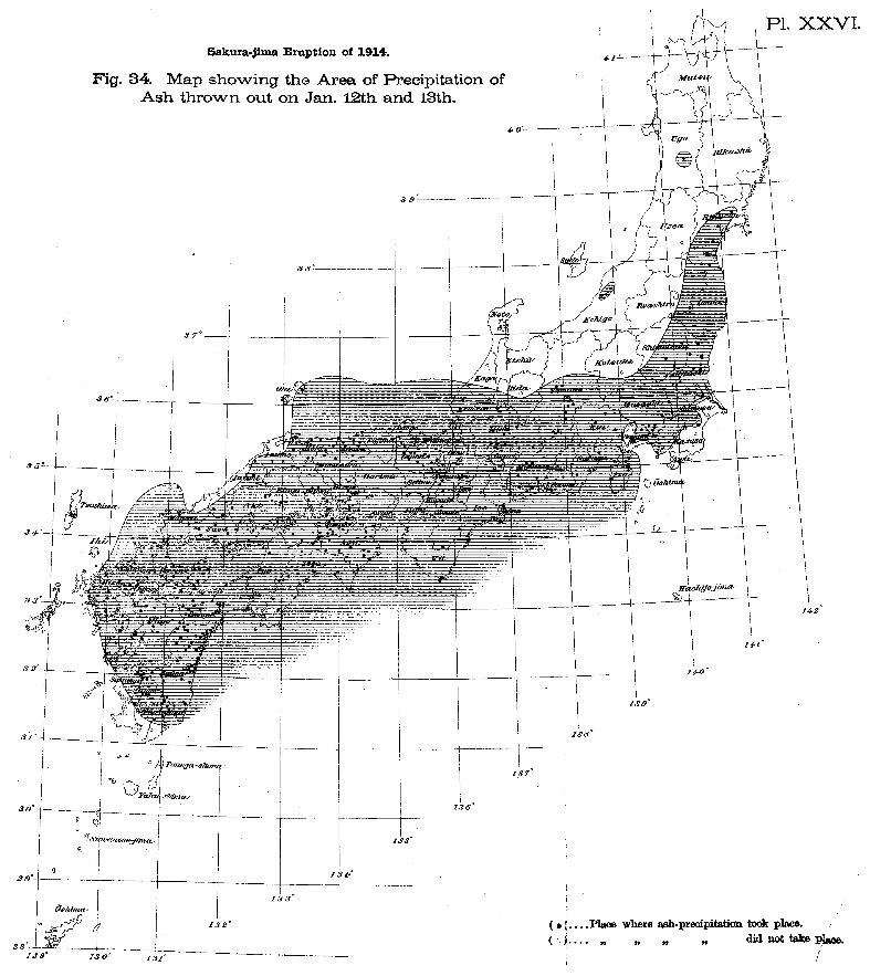
Figure 1 Map of ash dispersal over all of Japan following the Taisho eruption (Omori, 1914).

3 Methods of data generation

3.1 Simulation of selected eruption scenario

We used a fixed volcanological scenario over an extended contemporary period recorded in the meteorological reanalysis dataset to capture the extended daily variability of ash dispersal from the Taisho eruption. The PUFF model is an ash tracking model developed during the Redoubt volcano eruption in 1989, and is known for its high resolution and accuracy results (Tanaka, 1994; Searcy et al., 1998; Scollo et al., 2011; Folch, 2012). We ran the PUFF model for 23 376 d from 1 January 1958 to 31 December 2021. This model considers ash as a collection of a finite number of virtual particles and computes their motion over time. It works best within the first 48 h of the eruption (Searcy et al., 1998; Tanaka, 1994). The PUFF model is a Lagrangian-based model with several advantages over other (Eulerian) approaches. Eight of the nine Volcanic Ash Advisory Centers (VAACs) worldwide, including Tokyo VAAC, operate models based on the Lagrangian approach (Folch, 2012; Lin et al., 2012). A recent study used the PUFF model to simulate the explosive eruptions of Sakurajima volcano 2017 and 2018 to assess its utility in forecasting real-time ash fallout, and produced satisfactory results.

Simulations agreed well with measurements recorded by instruments at several points near the volcano (Tanaka and Iguchi, 2019). Here, we construct the model using many random variables r_i(t), where $i=\mathrm{1}\sim M$ and M is the total number of particles. $r_i\left(t\right)=\left(x,y,z\right)$ represents the position vector for the i^th particle at time t with its origin at the volcano vent. Using the discrete-time increment Δt=300 s, the governing equation can be written as

$$\begin{array}{}\text{(1)}& \left\{\begin{array}{ll}{r}_i\left(\mathrm{0}\right)=S_i,& i=\mathrm{1}\sim M,\text{for}t=\mathrm{0},\\ r_i\left(t+\mathrm{\Delta }t\right)=r_i\left(t\right)& i=\mathrm{1}\sim M,\text{for }t>\mathrm{0}\\ +V\mathrm{\Delta }t+Z\mathrm{\Delta }t+G\mathrm{\Delta }t,& \end{array}\right.,\end{array}$$

where S_i is the initial location of all the particles at the vent, $V=(u,v)$ is a vector for the wind velocity moving the particles and $Z=(c_h,c_h,c_v)$ is a vector for the diffusion velocity containing the diffusion speeds generated by Gaussian random numbers. $G=(\mathrm{0},\mathrm{0},-w_t)$ is the gravitational fallout velocity obtained by approximating the extended Stokes law for various particle sizes (Tanaka, 1994; Tanaka and Yamamoto, 2002). The movement of particles steers the diffusion Z Z-direction, and the size of the particles affects the gravitational fallout G (Searcy et al., 1998; Tanaka, 1994). The diffusion speed c (c_h or c_v) was obtained by the random walk process related to the diffusion coefficient K as $c=\sqrt{\mathrm{2}K}/\mathrm{\Delta }t$ (Tanaka et al., 2016; Tanaka and Iguchi, 2019). Tanaka and Yamamoto (2002) conducted several diffusion tests with various values of K, and compared the results with satellite images of actual dispersals from several volcanic eruptions in the past. Based on this research, we assigned a suitable horizontal diffusion coefficient K_h= 150 m² s⁻¹ and vertical diffusion coefficient K_v= 1.5 m² s⁻¹ (Table 1).

Table 1 Input values for the simulations used in this study.

These diffusion coefficients are consistent with the in situ observations documented by Eliasson et al. (2014) and adjusted for the Sakurajima volcano. The values used here follow those reported by Tanaka et al. (2016) and Tanaka and Iguchi (2019) but are smaller than those reported by Fero et al. (2008, 2009) and Kratzmann et al. (2010). To further investigate the ash dispersal process to distal locations in all Japan, we extended the simulation period of the PUFF model to 96 h after the eruption began. Following Eq. (1), by modelling the source location of the volcano vent as $S\left(x,y,z\right)$, we can adjust the number of particles released at each time step to obtain the optimal statistical information from the model.

For each time step, we assigned a Gaussian random number for each particle (M₀) and scaled it according to the emission rate, making the value of the total number of particles (M) change linearly with the emission rate (Tanaka et al., 2016). We assigned the initial number of particles to 5000 due to constraints in the available computational power. The size of volcanic ash varies from fine ash to boulders. Large particles tend to settle out quickly so airborne particle size decreases over time. Therefore, each ash particle will have a different grain size (Bonadonna et al., 1998), and we assume that each particle has an initial grain size following a logarithmic Gaussian distribution with a standard deviation of 2.0 centred at −3.0. Thus, the average particle size was approximately 1.0 mm on a log scale, with 68 % of the particles within the range of 10 µm–10 cm (Table 1). Given the initial vertical velocity of the emission with specified damping (e-folding) time τ₀, the particles are distributed randomly in a vertical manner from the vent z₁ to the plume's peak z₂ continually. Then, using time integration for the vertical velocity in the momentum equation, we obtained the final form as z(0)=z₁ and z(t)=z₂ during time step Δt (Tanaka et al., 2016).

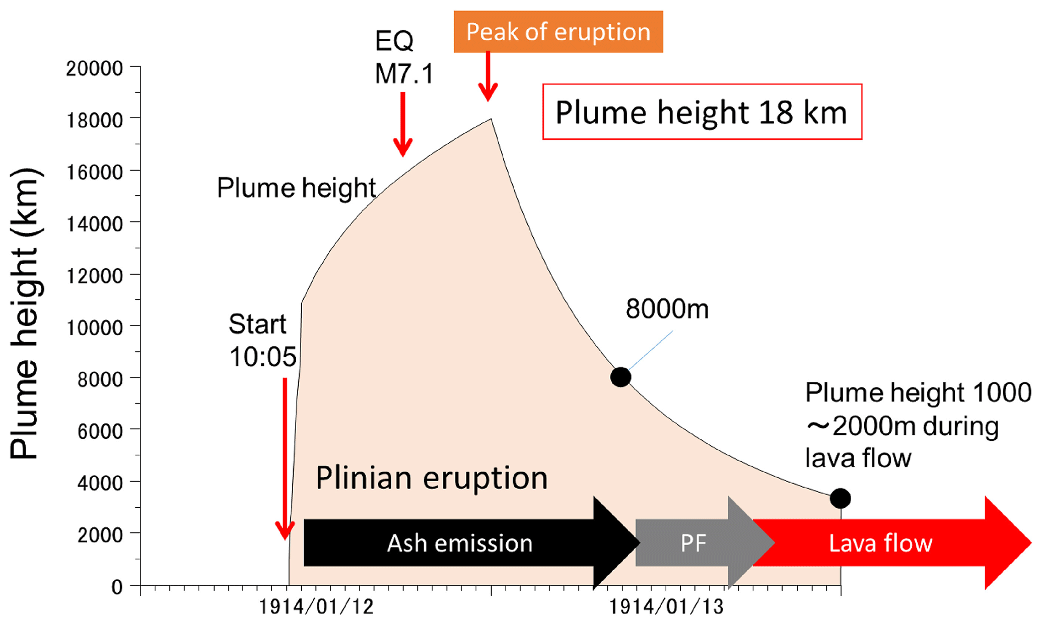
Figure 2 Plume height progression during the Taisho eruption on 12–13 January 1914 with information on both subsequent events and materials ejected. PF means pyroclastic flows that occurred from 13 January 1914 (Takebayashi et al., 2021).

3.2 Estimation of mass eruption rate based on plume height transitions

We used the estimated emission rate of Iguchi (2014), based on a previous study (Kobayashi, 1982). We consider the maximum estimated plume height as 17 890 m around midnight on 13 January 1914, which is close to the range of plume heights in the historical chronicles (Sect. 2; Fig. 2). We obtained the value of the mass eruption rate (ε) and the mean eruption mass (Table 1) with the help of temporal change in plume height. The obtained values agreed well with a recent observation (Todde et al., 2017). The pressure of a reservoir that ejects gas through a nozzle (P_(t)) at time t decays exponentially with time (Nishimura, 1998) following Eq. (2):

$$\begin{array}{}\text{(2)}& P_{\left(t\right)}=\mathrm{\Delta }{P}_{\mathrm{0}}{\left[\mathrm{1}+{\displaystyle \frac{\mathit{\gamma }-\mathrm{1}}{\mathrm{2}}}{\left({\displaystyle \frac{\mathrm{2}}{\mathit{\gamma }+\mathrm{1}}}\right)}^{\frac{\mathit{\gamma }+\mathrm{1}}{\mathrm{2}\left(\mathit{\gamma }-\mathrm{1}\right)}}{v}_{\mathrm{0}}{\displaystyle \frac{A}{\mathrm{Vol}}}t\right]}^{\frac{-\mathrm{2}\mathit{\gamma }}{\mathit{\gamma }-\mathrm{1}}},\end{array}$$

where Vol is the volume of the reservoir, A is the cross-sectional area of the nozzle, v₀ is the initial ejection velocity, P₀ is the initial pressure, and γ is the specific heat ratio (values within the range 1.01–1.4). Because the Taisho eruption is a Plinian eruption, the plume height (H) is proportional to a quarter of the power of the heat discharge rate $\left(\frac{\mathrm{d}Q}{\mathrm{d}t}\right)$ (Morton et al., 1956). Assuming that the volume of the reservoir is much larger than the ejected gas volume, the mass eruption rate (ε) is equivalent to the decay rate of the pressure ($\frac{\mathrm{d}P}{\mathrm{d}t}$), which can be estimated from the changes in plume height as follows:

$$\begin{array}{}\text{(3)}& H\propto {\left({\displaystyle \frac{\mathrm{d}Q}{\mathrm{d}t}}\right)}^{\mathrm{1}/\mathrm{4}}\propto {\left(\mathit{\epsilon }\right)}^{\mathrm{1}/\mathrm{4}}=k{\left({\displaystyle \frac{\mathrm{d}P}{\mathrm{d}t}}\right)}^{\mathrm{1}/\mathrm{4}}.\end{array}$$

3.3 Long-term wind field

Long-term weather data from meteorological reanalysis are necessary inputs to long-term ash transport simulation, as the wind strongly affects the sedimentary properties of volcanic ashfall (Hattori et al., 2013, 2016; Poulidis et al., 2018). One available long-period historical dataset is the JRA-55 reanalysis dataset, which includes the global meteorological reanalysis dataset from 1958 to the present, developed by the Japan Meteorological Agency (JMA) to study long-term variations in atmospheric and climate phenomena. The JRA-55 employs a reduced Gaussian horizontal grid system and applies a vertically conservative semi-Lagrangian advection scheme (Kobayashi et al., 2015). We utilised the JRA-55 data for the PUFF model, considering the horizontal wind grid to be 1.25^∘ × 1.25^∘. We employed 16 vertical layers from 1000 to 10 hPa atmospheric pressure, and we used these data at four time points (00:00, 06:00, 12:00, and 18:00 UTC) daily. The 3D wind field consisted of zonal wind (U), meridional wind (V), and geo-potential height (gph), which were interpolated to the position of each ash particle in space and time using the cubic spline method.

The ash dispersal from the Taisho eruption was controlled by the westerlies (250 hPa) and surface winds (1000 hPa) (See Sect. 2). The most frequent directions at upper altitude winds are from W and SW, which are strongest during winter and weakest in summer. During winter and spring, winds mostly come from west, and the southwesterlies are more prominent in summer and autumn. Meanwhile, weaker winds dominate on the surface with distinct directions during cold seasons (autumn and winter), which blow from WSW–SW and NNE–NE direction, and warm seasons (spring and summer), where the winds are just southwesterly. Wind conditions depend on season (Fig. 3) so ash deposition depends on season of the eruption (Biass et al., 2017; Poulidis and Takemi, 2017; Poulidis et al., 2018).

3.4 Recording ashfall location and thickness

This study considers the ashfall deposits on the ground as particles with non-positive altitudes, with their location marked as a longitude–latitude pair. For each simulation, as the computation progressed, the particles with a negative value in the altitude dimension were subset to other files before being compiled when the simulation was completed. During this process, we captured the rest of the flowing particles as airborne ash concentrations, copied them to different files, and saved them using time marking every 90 min.

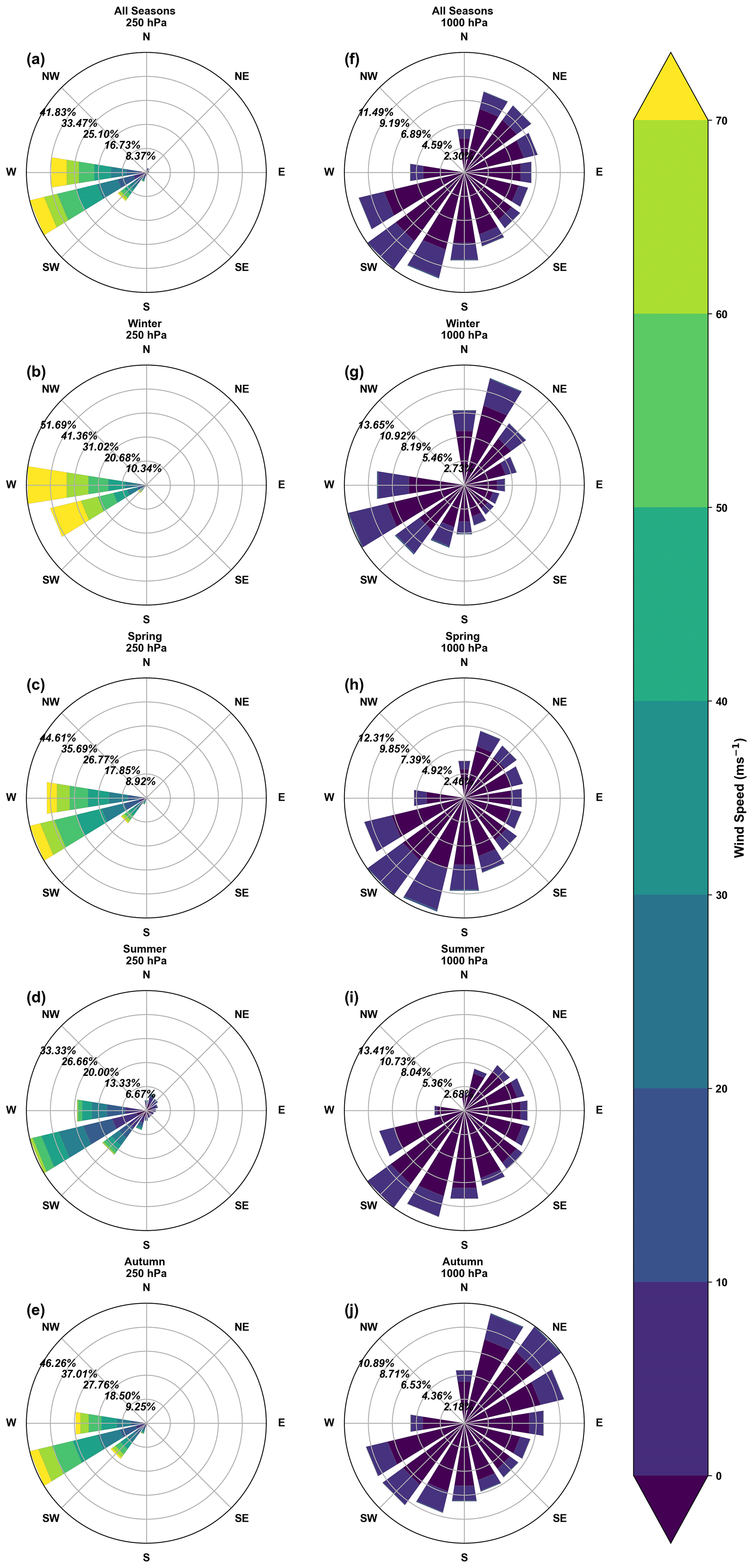
Figure 3 Ten wind roses illustrating wind conditions inferred from the JRA-55 Reanalysis dataset (Kobayashi et al., 2015) for upper altitude winds (first column) and surface winds (second column). (a, f) 1958–2021; (b, g) winter, (c, h) spring, (d, i) summer, and (e, j) autumn. Roses indicate the probability of the provenance and sequential colours indicate the speed gradients.

We separated the measurement of the ashfall deposit and airborne ash concentrations into two files using this mechanism. Furthermore, we measured the ashfall thickness (ashfall depth) by dividing the surface area by the ashfall density according to its particle size. First, we allocated the ashfall particles to grids according to their location. Then, we set all ashfall particles in those grids according to their average values. We considered all the adjacent grids and the pre-assigned mass values multiplied by the number of particles to obtain the total mass of the ashfall deposit. It is possible to obtain the mass of each particle based on the particle size. However, because we deliberately designate the total initial number of particles as a constant number and smaller than the actual number in the real case, the total mass of all particles is less than the actual mass, and the difference may increase as the scale of the eruption increases. Therefore, considering the particle size under total mass conservation, the virtual mass of each particle is necessary (Shimbori et al., 2009). When the eruption reached its peak, each ash particle contained approximately 450 tons of virtual mass. This method alleviated the uncertainty that appears when assigning a small number of particles in the simulation (Scollo et al., 2011). After assigning the virtual mass to each particle in one grid, the thickness of the ashfall χ_ij at grid i,j obtained from the following equation:

$$\begin{array}{}\text{(4)}& {\mathit{\chi }}_{ij}={\sum }_n{\displaystyle \frac{\stackrel{\mathrm{̃}}{m}\left(D_n\right)}{\mathrm{\Delta }x\mathrm{\Delta }y}},\end{array}$$

where $\stackrel{\mathrm{̃}}{m}$ is the total virtual mass for the total n particles within the grid i,j of area ΔxΔy corresponding to the particle size D_n (Shimbori et al., 2009). All computations (running the simulation, processing wind fields, and computing the total ashfall accumulation on the ground) were performed by a workstation with 32 GB RAM, dual 16-cores Intel Xeon E5-2620V4 2.10 GHz processors, and 4 GB NVIDIA Quadro P1000 GPU.

4 Dataset overview and usage examples

4.1 Data description and availability

The dataset contains three data series:

1. Ashfall deposit measurements from 128.5 to 148.6^∘ E and 30.0 to 45.9^∘ N in 0.1^∘ × 0.1^∘ grid (approximately 10 km²) (1958–2021).

2. Ashfall deposit measurements from 129 to 132^∘ E and 30.5 to 32.5^∘ N in 0.01^∘ × 0.01^∘ grid (approximately 1 km²) (1958–2021).

3. The time series of the total airborne ash concentrations in the air every 90 min (1958–2021).

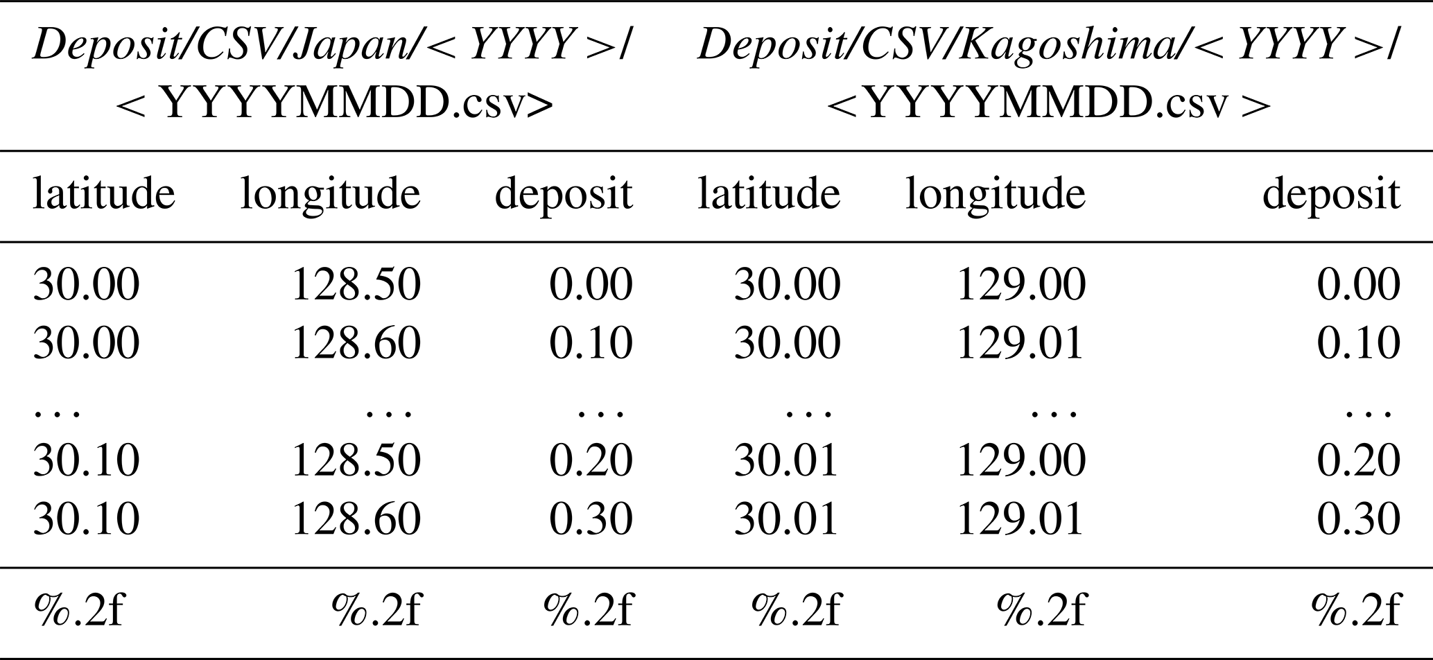
To ensure maximum availability for diverse users of the dataset, we prepared it in two formats: a space-separated ASCII table in comma-separated value (CSV) format (Table 2) and a multi-dimensional array structure in the Network Common Data Format (NetCDF).

NetCDF is useful for supporting access to diverse types of scientific data, and its files are self-describing, network-transparent, directly accessible, and extensible (Unidata, 2021). We developed the NetCDF files using the Xarray library in Python using the NETCDF4 package (Hoyer and Hamman, 2017). Owing to the high dimensionality of the airborne ash concentrations, we only provided these data in the NetCDF format. Ashfall deposit data are available in CSV and NetCDF formats. The name of each file was set to the simulation date in ISO-8601 format (YYYYMMDD≪.csv, .nc≫), and files were stored inside a directory named by year (YYYY) within each region (Japan and Kagoshima). Each dataset contains an ordered set of location markings (longitude, latitude) and ashfall depth (in cm), which are stored in two decimal floating-point formats. The location markings are the coordinates of the ashfall deposit in NetCDF data format. The airborne ash concentrations are the total number of particles at a specific location and time. The tracking period of the ash particles began 90 min after the simulation and was completed after 96 h. As the three-dimensional shape of the affected area and the total number of particles change throughout the time dimension, we assigned date_time as the primary coordinate. The dataset directory consists of two folders based on the data observations: Airborne and Deposit. The Deposit folder contains two child directories based on the data format and observation range, which break down to every year from 1958 to 2021. The Airborne dataset has a straightforward directory structure (year, YYYY) because it consists of one data format without a separate observational range. Detailed structure of the dataset for both the ground deposits and airborne concentrations is provided in the Appendix A.

Table 2 Tabular view of sample deposit data for two regions: Japan and Kagoshima. Each column is separated by a comma, corresponding to CSV format.

The dataset is available at the DesignSafe-CI Data Depot (https://www.designsafe-ci.org, last access: 31 July 2020) hosted at the Texas Advanced Computing Center (TACC). This data depot is provided by the Natural Hazards Engineering Research Infrastructure (NHERI), which provides the natural hazards engineering community and researchers with state-of-the-art cyberinfrastructure (Rathje et al., 2017).

The dataset can be accessed directly at https://www.designsafe-ci.org/data/browser/public/designsafe.storage.published/PRJ-2848v2 or through the DOI: https://doi.org/10.17603/ds2-vw5f-t920 (Rahadianto and Tatano, 2020). When accessing the dataset from the DOI, the link will direct to Version 1 instead of Version 2; please select an appropriate version for the latest updates. Users can access the dataset without prior registration and may choose any data to download. Data can be downloaded as a single file or a collection of multiple files.

4.2 Usage examples of the dataset

The dataset comprises ash deposits on the ground and airborne concentrations of a typical large-scale eruption at Sakurajima volcano (Sect. 2) for an extended period. The data can be used to prepare a response for an ashfall disaster. Here, we demonstrate how to use these data to create conditional ashfall hazard maps. The information in such maps serve as a reference for designing an early warning system, planning ash clean-up operations, managing closures of air and land transportation, and preparing long-term long-distance evacuation strategies. The maps describe the probability distribution of exceeding a selected hazard threshold based on the statistical distribution of the wind profiles (Bonadonna, 2006).

Figure 4 Probability distribution of ash dispersal with the threshold for airport closure risk (≥ 0.02 cm). Airport locations are marked by black aeroplane icons and the busiest airports by larger red icons. The colour gradient shows the probability of ash deposits exceeding the threshold. Human geography base (ESRI, 2022) provided the basemap for this figure.

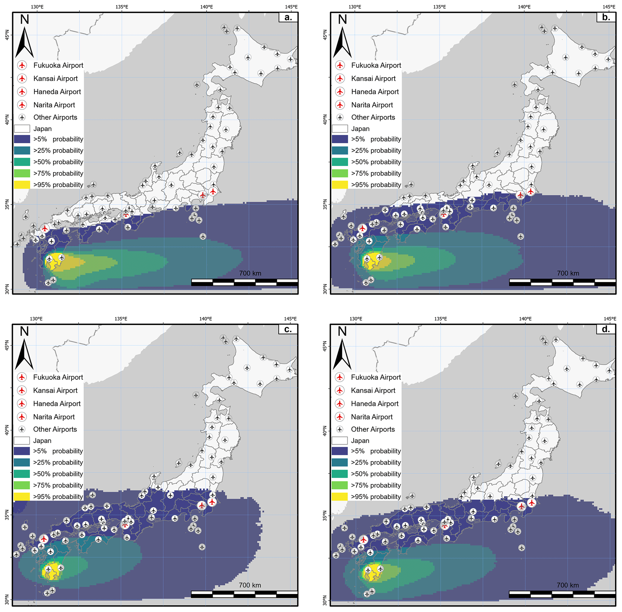
Figure 5 Seasonal probability distribution of ash dispersal with the threshold for airport closure risk (≥ 0.02 cm). The panels show the probability distribution of ash dispersal during (a) winter, (b) summer, (c) spring, and (d) autumn. Airport locations are marked by black aeroplane icons and the busiest airports by larger red icons. The colour gradient shows the difference in the probability of ash deposits exceeding the threshold. Human geography base (ESRI, 2022) provided the basemap for this figure.

Several researchers used such maps to illustrate hazard assessments of a specific volcanic eruption scenario, identify the possible impacts of the assumed maximum expected events, and quantify the probability of first-order impacts on built environments (Bonadonna, 2006; Biass et al., 2014, 2016). One example is a conditional ashfall hazard map showing airport closure risk of all of Japan for all the wind profiles used in the simulation (Fig. 4). The threshold, or hazardous limit, of all hazard maps in this subsection is defined the Cabinet Office's Working Group on Wide-Area Ashfall Countermeasure at the time of Large Eruptions, Central Disaster Management Council, Executive Committee for Disaster Prevention (2020). We used a 0.02 cm threshold for ash on the airport's runway that would disrupt the take-offs and landing sequence of aeroplanes (Figs. 4 and 5). The busiest airports in Japan are Fukuoka, Kansai, Haneda, and Narita (Ministry of Land, Infrastructure, and Tourism, 2022).

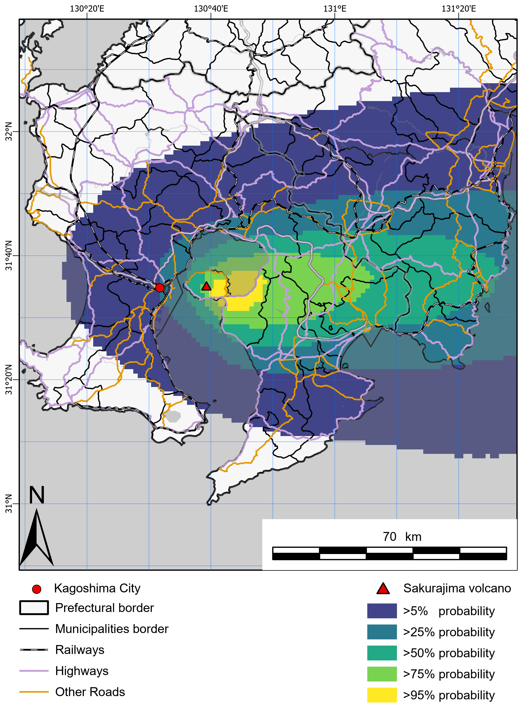
Figure 6 Probability distribution of ash dispersal with the threshold for road closure risk (≥ 3 cm). Black and white stripes mark railways, and highways and other roads are coloured lines. The colour gradient shows the probability of ash deposits exceeding the threshold. Human geography base (ESRI, 2022) provided the basemap for this figure.

Figure 7 Seasonal probability distribution of ash dispersal with the threshold for road closure risk (≥ 3 cm). The panels show the probability distribution of ash dispersal during (a) winter, (b) summer, (c) spring, and (d) autumn. Black and white stripes mark railways on the map, and highways and other roads are coloured lines. The colour gradient shows the probability of ash deposits exceeding the threshold. Human geography base (ESRI, 2022) provided the basemap for this figure.

In average, a large-scale eruption in Sakurajima volcano would affect many airports from south to east, with the busiest airports having more than 5 % probability of closure after an eruption, possibly displacing numerous passengers and inflicting economic losses. The dataset can also be used to portray the seasonal variations in the airport closure risk (Fig. 5). For example, a large eruption during summer would have greatest impact on the number of airports, and an eruption during autumn would also disrupt traffic at Japan's busiest airports. Further analysis of the airborne concentration data can inform the timing of ash arrival in some airports that would inform how to protect or evacuate aircraft if there was sufficient time. The variety of geographical dimensions offered by the dataset also allows investigation of the immediate consequences of ground ashfall deposits in urban areas surrounding the Sakurajima volcano. Analogous conditional ashfall hazard maps can be made for the risk of disruption to land transportation network (Figs. 6 and 7). We used a 3 cm threshold as the hazard limit for closing roads and railways when they would be impassable by cars and trains. The figures illustrate how a large-scale eruption of Sakurajima volcano could severely affect the eastern parts of Kagoshima City (located downwind of the volcano) with more than 25 % probability, regardless of eruption time. The data also show how the seasonal patterns determine the extent of the ash deposits in the western parts of South Kyushu, with a large-scale eruption in summer would be escalating the damage to almost the entire Kagoshima Prefecture. The projected intensity of the ashfall hazards to the transportation networks provide insights for preparing responses and countermeasures. These preparations include scheduling roads and highway blockages, designing evacuation strategies, and managing the ash cleaning process shortly after the eruption.

5 Validation and limitations

5.1 Validation

Simulation results have been validated using methods that include comparison to post-event reports, matching the ash cloud trajectory with satellite images, and adjusting the model's input to find the best-fit values (Webley and Mastin, 2009; Folch, 2012); for example, PUFF model simulations of the 1980 eruption of St. Helens, 1991 eruption of Hudson volcano, 1991 eruption of Mt. Pinatubo in the Philippines, 2001 eruption of Mt. Etna in Italy, 2006 eruption of Mt. Augustine, and all eruptions of North Pacific volcanoes from 1970–2010 (Fero et al., 2008, 2009; Kratzmann et al., 2010; Webley et al., 2008; Scollo et al., 2011; Webley et al., 2012). Several past studies validated ash dispersal simulations using the PUFF model for smaller-scale eruption of the Sakurajima volcano (Tanaka and Iguchi, 2019; Tanaka et al., 2020). The PUFF model has never been validated for historical large-scale eruptions of Sakurajima volcano, with its great plume height, eruption volume, and range of ash deposition. Ideally, if precise wind data at the time of the selected eruption are available, we can replicate the eruption; therefore, simulation results with similar wind patterns to the eruption would resemble the historical reports. The dataset presented here offered an opportunity to validate the simulation of ash dispersal from a large-scale eruption of Sakurajima volcano over all Japan. We directly compared selected simulation results with the available reports of the Taisho eruption. However, making a direct comparison with the ground truth data was challenging owing to the following:

1. A lack of complete ground reports. Available reports from cities and tobacco plantations across Japan mentioned subjective ash deposit observations without a quantitative measurement, e.g. “frost-like ash”, “house roof become white”, and “slight deposit”.

2. A lack of complete wind data at the time of eruption. Only surface observations are available at limited observation points, and it is not possible to completely replicate the ash transport process.

Despite these limitations, we attempted to utilise an innovative approach to use all available information to validate the dataset. The ash dispersal map (Fig. 1) provided locations of ash deposition across all of Japan, and the detailed weather conditions that control the ash dispersal process are available. We utilised these data for validation as follows:

1. We manifested the ground data in the same dimension as the simulation output by digitally redrawing the ash distribution map for all of Japan, provided by Omori (1914), using geographic information software (GIS). The resultant ground observation data resembled the original ash distribution of the Taisho eruption (Fig. 8).

2. We found wind pattern in the wind data of the JRA-55 Reanalysis that are equivalent to the day of the eruption. We expected that the similarity in weather features would also match a similar wind profile across multiple atmospheric levels. We subset the number of simulation results for validation checking with the data produced in the previous step.

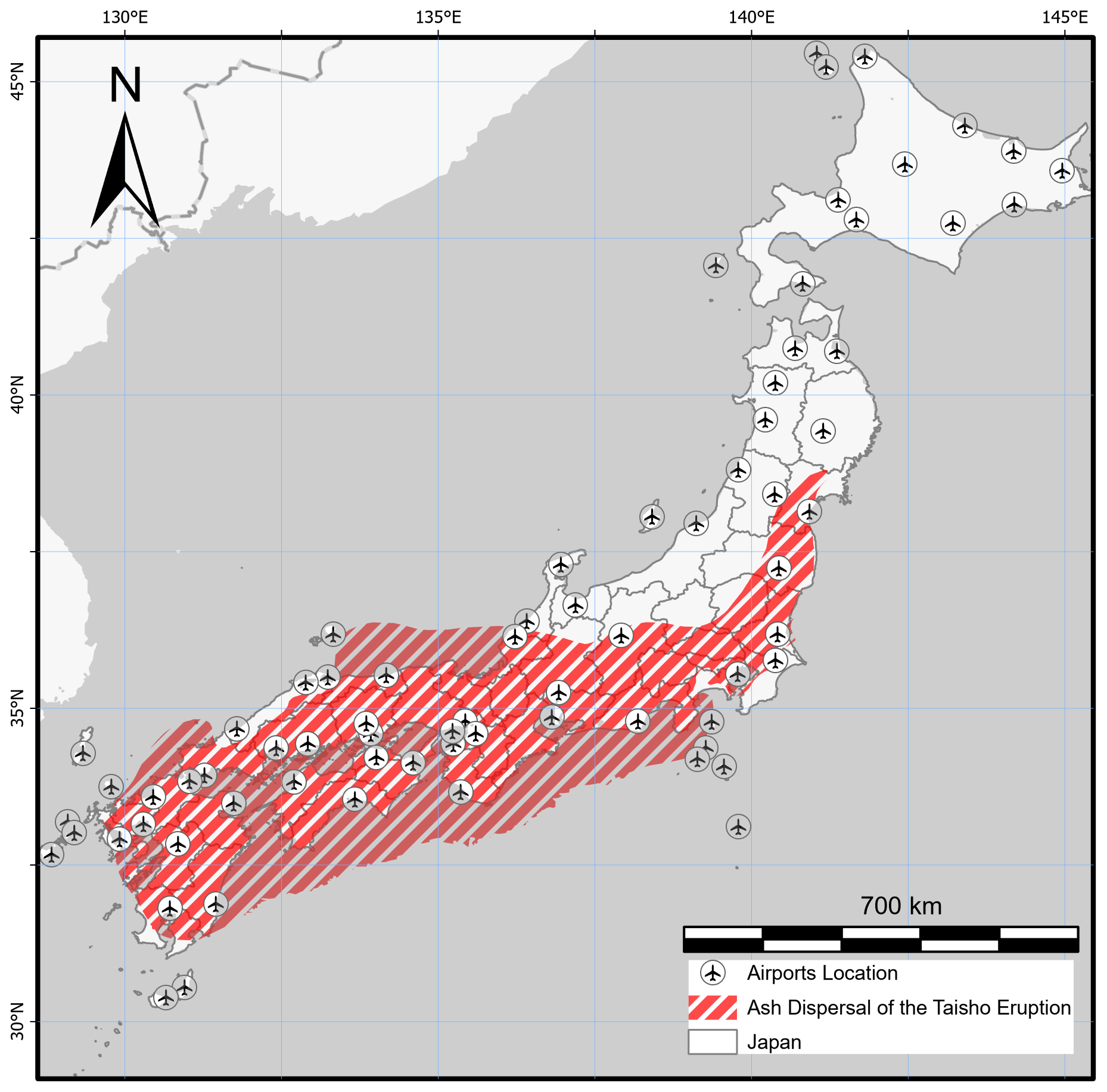
Figure 8 Transformed ash dispersal map using ArcGIS software with airport icons for impacts reference. Human geography base (ESRI, 2022) provided the basemap for this figure.

Appendix B provides the detailed explanation of each step. The simulation result of the chosen date was matched with the new ground data using a binary contingency matrix (Table 3). The evaluation focused on measuring how the ash dispersal map produced from the simulation on selected dates would cover an equivalent region of interest to the ground data. We limited the evaluation to all ash deposits on the land and omitted ash deposits on the sea. We quantified the hit rate score, Hit, of the simulation matching in the binary contingency table as follows:

$$\begin{array}{}\text{(5)}& \mathrm{Hit}={\displaystyle \frac{\mathrm{TP}+\mathrm{TN}}{\mathrm{TP}+\mathrm{TN}+\mathrm{FP}+\mathrm{FN}}}.\end{array}$$

For brevity, we chose only the top date of the semantic textual similarity (STS) scores list in Appendix B (5 March 1997) in the matching process. The simulation for the chosen date reached satisfactory performance with a high Hit score (0.832), indicating that the selected date with weather conditions similar to those of the Taisho eruption had a reasonably similar ash dispersal pattern. Figure 9 exhibits further evidence of similarities in the ash dispersal map for the selected simulation results.

Table 3 Binary contingency table for the validation.

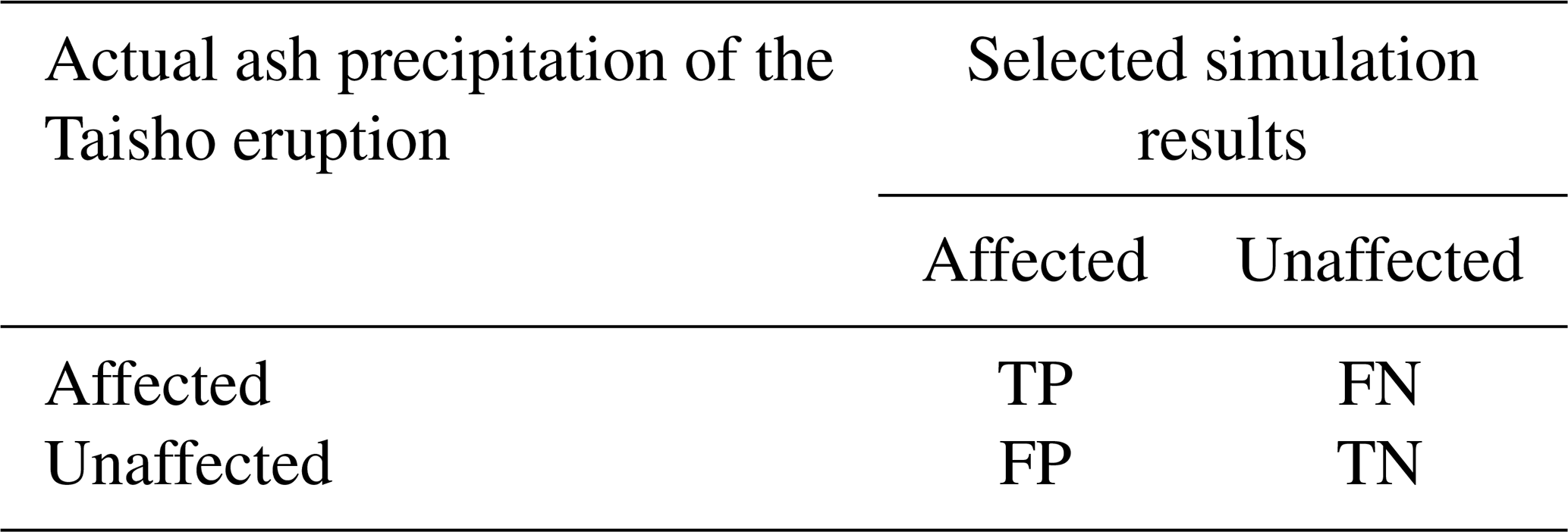
TP, true positive; TN, true negative; FP, false positive; FN, false negative.

5.2 Dataset limitations

Generally, results from the simulation of volcanic ash dispersal and transport models depend on the initial values of parameters of eruption source and wind conditions during the eruption. These parameters are critical in determining the impacts of ashfall on proximal and distal locations (Bonadonna et al., 2012; Folch, 2012; Macedonio et al., 2016; Mastin et al., 2009; Webley and Mastin, 2009). We used deterministic values of plume height, erupted mass, and mass eruption rate as the eruption source parameters. We utilised the calculation by Iguchi (2014), incorporating the study by Morton et al. (1956) for the relationship between the observed plume height in the historical reports and studies (Kobayashi, 1982; Koto, 1916; Omori, 1914; Todde et al., 2017) to produce the mass eruption rate. The change in plume height over time was positively correlated with the total eruption mass and eruption rate. However, the method introduces a significant bias in the mean height value. The eruption rate is roughly proportional to the fourth power of height.

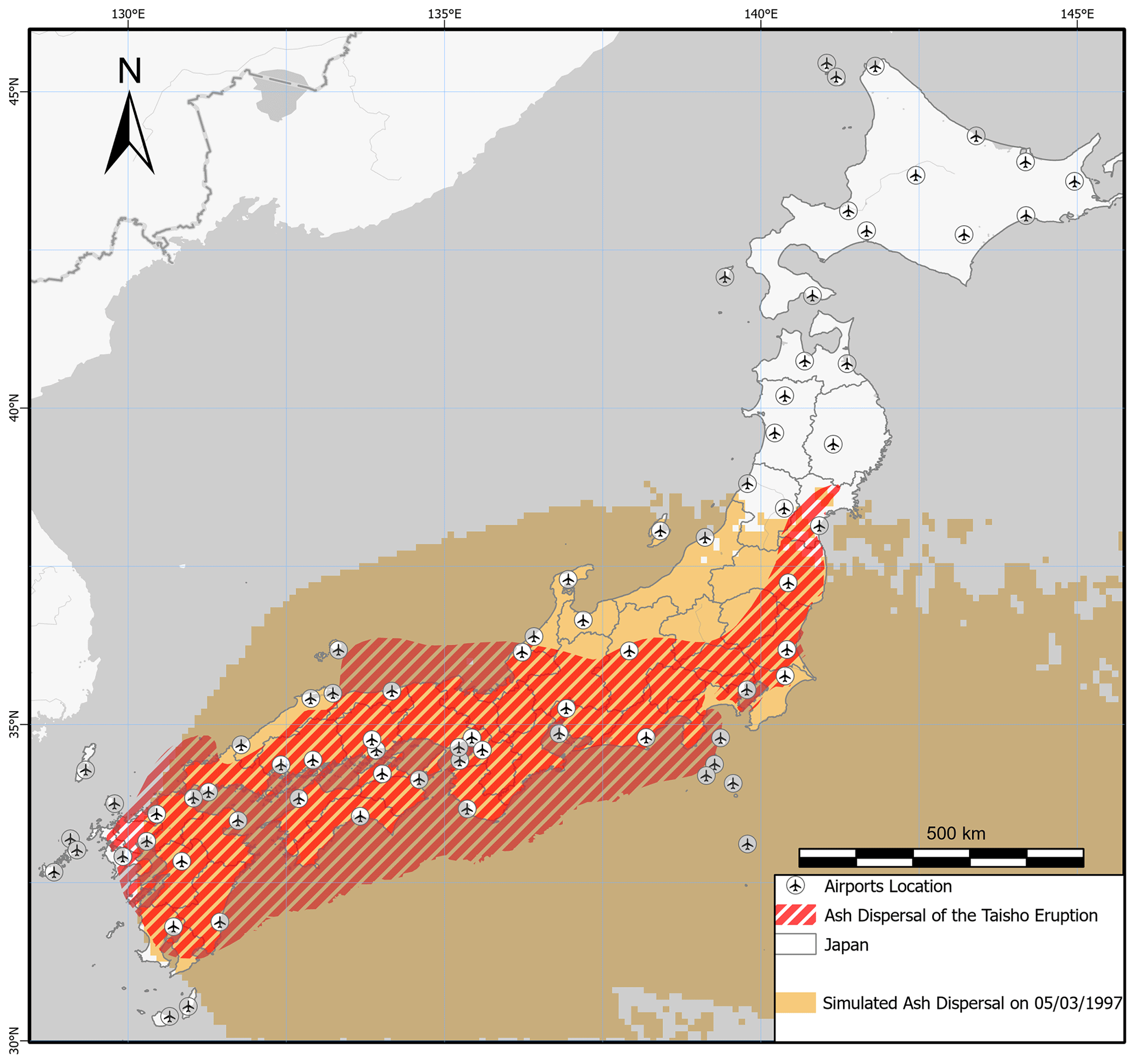
Figure 9 Comparison of ash distribution on the selected date (5 March 1997) according to the original ash dispersal map and simulation results. Human geography base (ESRI, 2022) provided the basemap for this figure.

Therefore, error in assigning the precise height will significantly affect its conversion to the eruption rate; and therefore, to the outcome of the simulation (Folch et al., 2012; Mastin et al., 2009). We assigned the parameters of the largest eruption size or plume height of the last eruption as a baseline of a conservative safety factor, although we recognise that the variability could change the significance of the implied hazard. The values used here agreed fairly well with the past observations, and the bias in the eruption source parameter should be small and not significantly affect the ash dispersal mechanism. However, variations in these parameters result in different eruption rates and total mass, resulting in different ashfall footprints. Future vent location and eruption style, size, and duration significantly affect the ashfall in proximal and distal areas (Bonadonna et al., 2012; Mastin et al., 2009; Selva et al., 2018). Furthermore some parameters, such as the diffusion coefficient, settling particle velocity law (see Table 1), orographic effects, and the lack of topographical data, need to be set arbitrarily causing discrepancies when using different variations depending on the model (Macedonio et al., 2016; Poulidis et al., 2017, 2018; Scollo et al., 2011). Finally, the distributions of total grain size and particle density and shape, and the chosen aggregation method, also affect the accuracy of model outputs (Bonadonna et al., 2012; Folch et al., 2010, 2012; Mastin et al., 2009; Selva et al., 2018). Here, the aim of the simulation was to characterise the Taisho eruption, eliminating variations in those variables because we used a fixed scenario as the worst case. Using fixed values for the eruption source parameters to precisely replicate the transition in the Taisho eruption is a limitation which restricts the possibilities of future events.

Hickey et al. (2016) illustrated how the current uplift situation is similar to that of the preceding eruption event, so our results could provide valuable input to authorities and stakeholders. The dataset provides a guideline for understanding how such a large explosive eruption would affect contemporary Japan. Inaccuracies also occur due to the effects of winds and atmospheric humidity and other factors (Folch et al., 2012; Mastin et al., 2009). Meteorological conditions determine the ashfall dispersion trajectory and deposit location (Macedonio et al., 2016). Reanalysis datasets are favourable because they have better accuracy than the forecast dataset (Folch et al., 2012). The variability in the meteorological databases (ERA-Interim, JRA-55, NARR, etc.) is relatively insignificant (Selva et al., 2018). This dataset, intended to provide guidance for a worst case scenario, may remain helpful in extending the present study toward ashfall risk analysis and decision-making. We argue that the dataset here is vital to support future researchers and emergency managers in analysing and planning responses to crises that may occur under a variety of conditions. These risk assignments are rough estimates applying to the most likely future eruption size and type at Sakurajima volcano. There might be inconsistencies in the dataset that introduce bias in the ashfall hazard and risk analyses, so future users should consider all these sources of uncertainty.

6 Data availability

The dataset contains ashfall deposit measurement (in CSV and NetCDF) and airborne ash concentrations (in NetCDF) at various spatial resolutions across Japan from January 1958 to December 2021. The dataset is publicly available at https://doi.org/10.17603/ds2-vw5f-t920 (Rahadianto and Tatano, 2020). When accessing the dataset from the DOI, the link will direct to Version 1 instead of Version 2; please select an appropriate version for the latest updates.

7 Conclusion

Ash dispersal products from large eruptions have devastating impacts on various sectors, in areas near the volcano and in distal locations. Emergency managers and crisis response planners need to acknowledge the compounded effect of ashfall deposits on the infrastructures to manage losses appropriately. This study presents a dataset that is useful for research and planning, focusing on the context of the entire country. This paper describes the process of generating a dataset based on the recent large eruption of Sakurajima volcano (the Taisho eruption) by simulating the eruption process over an extended period from 1958 to 2021. We validated the simulation of ash dispersal over all Japan following a large-scale eruption of Sakurajima volcano within some limiting constraints. Finally, although it contains some degree of inaccuracies, the dataset can be used for further studies in ashfall risk analysis and decision-making, and will support future researchers and emergency managers in devising disaster responses for different conditions.

Appendix A

The structure of the dataset in NetCDF format is shown in Fig. A1 (ground deposits data) and Fig. A2 (airborne concentrations data).

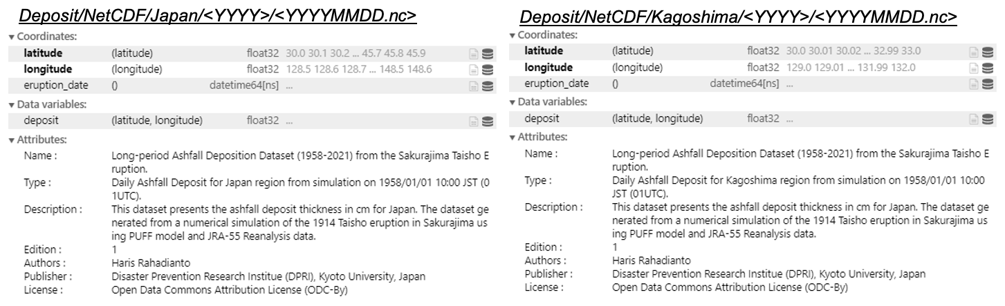
Figure A1 Structures of sample deposit data in NetCDF format. Left: all Japan, Right: Kagoshima region.

Figure A2 Structures of sample airborne data in NetCDF format.

Appendix B

A diagram explaining the flow of the validation procedure for this study is portrayed in Fig. B1.

B1 Transforming the original ash precipitation map

To transform ground data to the same area dimension as the model output to enable its directly comparison with simulation results, we digitised the 1914 ash dispersal map of Fig. 1 by placing binary markings to indicate the affected regions; i.e. 1 for red-striped grids and 0 for the rest.

All the binary values have a pair of longitude–latitude values to represent their positions on the map (Fig. B1. We added current airport locations to emphasise the impacts of ​​​​​​​​ ​​​​​​​​ very fine ashfall across all Japan. We used ArcGIS software with a WGS 84 projection (ESRI, 2017).

B2 Finding the identical weather characteristics

The weather at the time of eruption determines the ash fallout trajectory. At the time of the Taisho eruption the weather was unusual, which explains why the ashfall moved unpredictably to distal locations. Previous analyses have not adjusted for the anomalous weather conditions that day (e.g. Biass et al., 2017, among many others). The Taisho eruption occurred in winter when mid-latitude cyclones were active. Stationary planetary waves generated by the land–sea contrasts and the flow over the Himalayas reinforce the tropospheric jet stream and the baroclinic wave. In Japan, the reinforced jet streams cause the westerlies at 250 hPa pressure to exceed 70 ms⁻¹. The winds in the tropospheric jet stream blow from the west throughout the year; they are strongest in winter and weakest in summer (Wallace and Hobbs, 2006). The Meteorological Research Institute of the JMA (JMA-MRI) further clarifies how the westerly wind traverses above the Sakurajima volcano all year long from west to east. The westerlies reach their peak velocity in January and then continue to weaken until their lowest speed in summer, before rising again (Maeda et al., 2012). This cycle runs for the entire year and is a determining factor for the ash dispersal pattern.

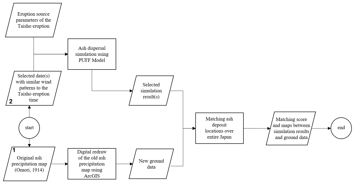
Figure B1 Flowchart of validation of the dataset. (1) Digitising the original ash precipitation map to become new ground data, and (2) selecting a simulation result for matching with ground observation data.

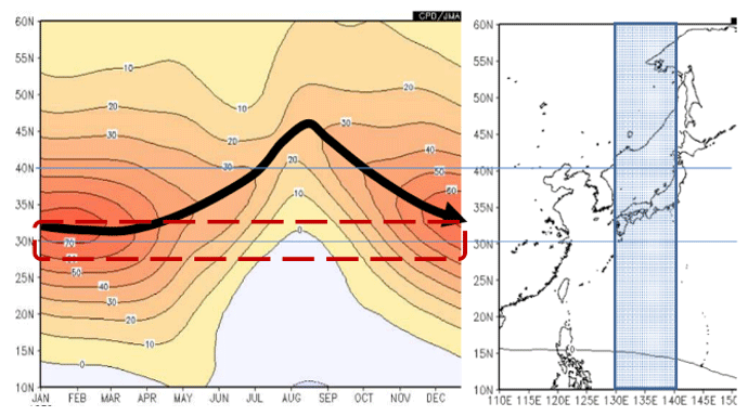
Figure B2 Seasonal progression of the westerlies over Japan at 12 km from the surface (Maeda et al., 2012). The red dashed square indicates the region covering Sakurajima volcano and Kagoshima city. The vertical axis shows the latitude of the wind position. The horizontal axis shows monthly changes of the wind velocity (left) and the longitude of the winds (right). The thick black arrow from left to right indicates the location of maximum velocity of westerlies based on seasonal progression. The straight blue lines indicate all regions in Japan affected by the westerlies. The small numbers inside the left image indicate the wind contour.

Figure B2 shows a time–latitude cross-section of the east–west wind at the 200 hPa (approximately 12 km from the surface), averaged at 130 to 140^∘ E based on the 30-year survey (Maeda et al., 2012; Mita et al., 2018). The Sakurajima volcano and its vicinity are situated around 31^∘ N (red dashed square), including Kagoshima City. Therefore, westerlies would usually bring most of the ashfall eastwards from the eruption. Instead, chronicles reported that ash traversed to the north, west, and southwest (Omori, 1914; Todde et al., 2017). This pattern contrasted with the preceding eruption (An'ei eruption – November 1779) that followed the pattern of the westerlies (Tsukui, 2011). Investigation of past patterns of ash dispersal from Sakurajima volcano also reaffirm the differences arising from seasonal features, agreeing that during winter, tephra should mostly go eastward and mostly fall in the Pacific (Biass et al., 2017; Poulidis et al., 2018; Mita et al., 2018).

When the Taisho eruption occurred, the vicinity of Kagoshima City and Sakurajima volcano experienced a maximum atmospheric pressure during the first 4 d, providing a unique characteristic of the Taisho eruption. From 9 January 1914 to the morning of 13 January 1914 atmospheric pressure in Japan was consistently recorded as unusually high, resulting in stable sea waves and low-velocity winds, indicating calm and clear weather in most places (Omori, 1914). Unexpectedly, the weak winds helped many people living near the volcano to evacuate by boat (Kitagawa, 2015). The eruption seemed to play a significant role in increasing the temperature in Kagoshima, but apparently the opposite was true (Omori, 1914). The leading cause of the high temperature at the time of eruption time was a sudden increase in southerly winds, as observed in Okinawa, 373 km from the vent (Omori, 1914). Furthermore, the chronicles of the tri-daily general weather conditions during the eruption reported that similar weather phenomena also occurred on 17 January 1914 (Omori, 1914). This vital information helped us derive a method for validating our simulation results. We concluded that clear, sunny weather with weak winds played a major role in transporting ashfall to all Japan.

Such conditions, although rare (less than 11 % as winds during winter are usually strong, see Fig. 3c), can recur. We assumed that the wind pattern would be similar on days with identical weather as irregular as the day of the Taisho eruption. We obtained wind data at various atmospheric pressure heights that matched the wind data during the eruption. Thus, the simulation on the dates with similar weather is expected to produce a similar ash distribution to all of Japan, comparable with the transformed ash dispersal map in Fig. 8. The Taisho eruption occurred in winter, so we searched for winter day(s) with weather conditions like the eruption day (12 January 1914). We searched the available weather information (from the chronicles and historical weather information provided by the JMA on their website) for clear sunny days with weak winds with high atmospheric pressure (anti-cyclonic) and higher temperatures during December, January, February, and March from 1 January 1958 to 31 December 2021. These features are quite distinct and rarely occur in Japanese winter. However, the Japanese authority only maintained surface weather data (temperature, pressure, humidity, precipitation, and wind speed) in a major meteorological observatory located in the capital of selected prefectures. These past data consist of daily and hourly observations. No other measurements were recorded at different atmospheric pressure levels. The surface weather chart on the day of the eruption (12 January 1914) and all simulation dates is available. Therefore, we utilised a surface weather chart for a clearer description of weather phenomena on a particular day. Weather charts consist of symbols and features that describe a particular meteorological pattern in a specific space–time dimension. Weather charts were created by plotting measurements including mean sea level pressure, wind barbs, and cloud cover, and identifying synoptic-scale features such as weather fronts. A meteorologist usually performs an isobaric analysis of the maps by constructing lines of equal mean sea level pressure (Wallace and Hobbs, 2006).

The weather chart at 06:00:00 on 12 January 1914 (Fig. B3) displays the high-pressure condition centred over central Honshu and covering almost all Japan. These local maxima in the pressure field explain the common weather characteristics in that specific region. The wind becomes stronger when the pressure gradient between the high- and low-pressure systems increases. Land friction weakens the wind coming from high-pressure systems. Hence, high-pressure systems typically result in weaker winds with clear skies and relatively warm weather (Wallace and Hobbs, 2006); thus, the interpretation of the weather chart corroborates the weather reports of the eruption day. Accordingly, searching for similarities in surface weather charts is appropriate for identifying identical weather conditions.

B2.1 Weather report commentary on the surface weather charts

To search for identical weather by comparing features in pairs of weather charts for similarity, we initially employed an image similarity method. However, this was very difficult, as the weather chart on the eruption day differed greatly from the modern weather chart used in Japan. The current daily weather chart differed from the weather chart on 12 January 1914 in the measurement time and scale of barometric pressure, dimension and projection of the map, and area included in the map. The format of daily weather charts in Japan has changed several times after World War II. In 1883 the JMA began producing daily surface weather charts for the Asia–Pacific region, which consisted of Japan and Japanese-occupied areas pre-World War II.

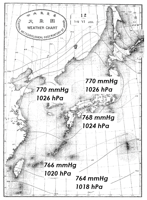
Figure B3 Weather chart at 06:00:00 on 12 January 1914, the time of the Taisho eruption, with additional markings of pressure measurement converted to the latest convention (mmHg → hPa). Modified from Omori (1914).

Since August 1958, the JMA has provided daily weather charts at various upper levels (500, 700, and 850 hPa) for the Asia–Pacific and 500 hPa for the Northern Hemisphere region. Since March 1996, the JMA added a daily surface weather chart for the Northern Hemisphere and a 300 hPa level for the Asia–Pacific region. Finally, in February 1999 the JMA updated all the weather charts and added a specific surface weather chart for the regions of Japan. These changes were accompanied by changes in the weather chart format to that currently in daily use. Owing to the ever-changing formats of past weather charts, identifying image similarity was time-consuming because of the need for multiple training data for every format to decide whether the two images are similar and was not feasible. Instead we utilised other information available in the daily weather charts, namely the general weather report commentary. Experts in meteorology developed this commentary as a guide to weather conditions during a particular day. Figure B4a portrays the weather report commentary on 12 January 1914.

All historical daily weather charts from 1883 to March 1938 have a written commentary explaining the weather conditions. However, this feature was omitted from April 1938 until December 1995. The JMA resumed the commentary feature in the monthly compilation of historical daily weather charts from January 1996 to date (Database of Weather Charts for Hundred Years, 2022) (Fig. B4b) (Japan Meteorological Agency, 2022).

The daily commentary usually includes the important weather characteristics such as high- or low-pressure centres or fronts, extreme weather phenomena such as typhoons, heavy rains, or heavy snow, and other special events such as disasters. This description enabled us to find weather similar to the day of the eruption during the dates used in the simulation (1996–2021, 3120 d). Several initial conversions were required to overcome a minor distinction between the old and modern commentaries, namely:

1. The old commentary on the weather chart on the day of the eruption was based on old Japanese syntax.

2. The old commentary addressed the weather in Japan and in Japanese-occupied areas.

We converted the old commentary to contemporary Japanese syntax (Table B1) and removed all observation areas outside the modern Japan region. The old commentary consists of three parts: the location of high- or low-pressure centres, the weather on the main islands of Japan (Honshu, Kyushu, and Hokkaido), and the weather in other parts of the Asia–Pacific under Japanese occupation. This commentary agrees with the meteorological reports provided in the chronicles (Omori, 1914). We focused on the weather on the main islands of Japan, and converted the old commentary to a form similar to that in the current daily weather charts.

The new phrases in the last column give more brief comments that match with the contemporary style in the modern weather charts while still maintaining the important features (high-pressure all over Japan, clear/sunny weather in the main islands, Kyushu is cloudy, and Hokkaido is either clear or cloudy with strong south-westerly winds). Then, we compared these phrases in contemporary Japanese with all the commentaries in the modern weather chart (from 1 January 1996 to 31 March 2021) provided by the JMA in winter (from January 1996 to March 2021), in the historical archive collected by the National Institute of Informatics (Database of Weather Charts for Hundred Years, 2022). These commentaries explain the weather conditions on a particular day in a random sequence; that is, not in a similar order to the processed commentary phrases (from 12 January 1914). Finally, we utilised the natural language processing (NLP) method to find semantic textual similarity between all commentaries with sentence embedding using SentenceBERT (Reimers and Gurevych, 2019).

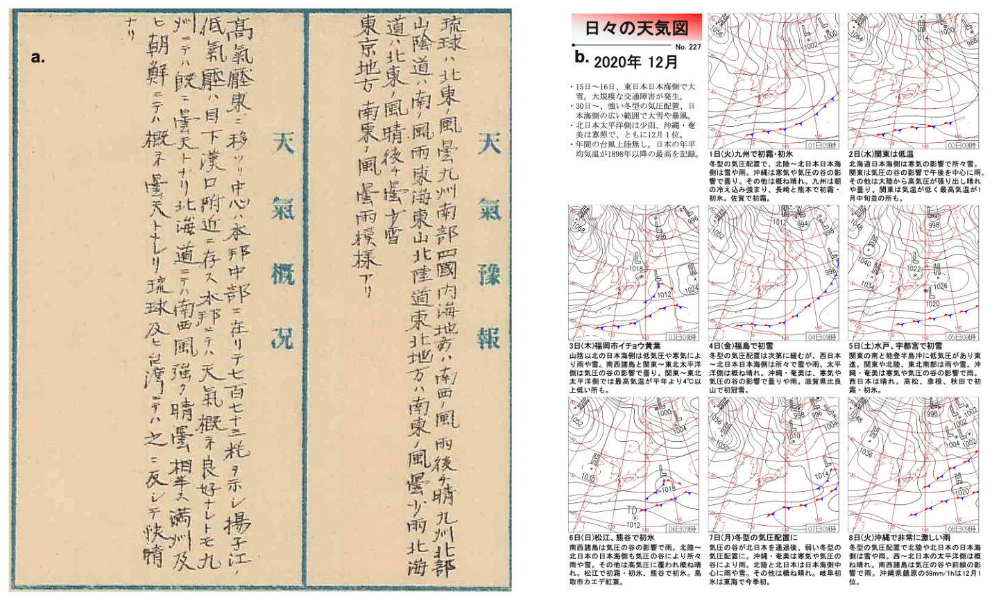
Figure B4 General weather report commentary on the weather condition inside the weather chart. (a) Old weather chart included the commentary on the bottom of the second page on the day of the Taisho eruption (Database of Weather Charts for Hundred Years, 2022). (b) Modern weather chart: the first page of the daily weather chart compilation for December 2020. The commentary is placed at the bottom of the monthly compilation of daily weather charts (Japan Meteorological Agency, 2022).

Table B1 Conversion of the general weather commentary in the weather chart of 12 January 1914.

B2.2 Semantic textual similarity of weather report commentary using SentenceBERT (SBERT)

To find similar weather, both commentaries should have a meaning that is semantically similar, regardless of the sentence structures and words used to form the sentence. The vast improvements in machine learning (ML) and artificial intelligence (AI) applied to NLP tasks allowed us to find the similarity between two sentences using semantic textual similarity (STS) by embedding all sentences first. Word embedding represents words in the form of real-valued vectors which encode the meaning of a word such that the words that are closer in the vector space will be similar in meaning (Jurafsky and James, 2000). Sentence embedding is the sum of individual word embedding (Cer et al., 2017). STS scores semantic similarity on a continuous scale (e.g. a vehicle and a car are more similar than a wave and a car) rather than binary (e.g. a vehicle and a car are the same, and a wave and a car are not the same). STS provides a unified framework that allows for the extrinsic evaluation of multiple semantic components.

This framework includes word sense disambiguation and induction, lexical substitution, semantic role labelling, multi-word expression detection and handling, anaphora and co-reference resolution, time and date resolution, named-entity handling, under-specification, hedging, semantic scoping, and discourse analysis (Agirre et al., 2012). Here, we considered a pair of sentences to be similar (in this case, the weather condition) if they were located close to each other, as both sentences are mapped to a dense vector space (Reimers and Gurevych, 2019, 2020). Google led the current state-of-the-art NLP development with its technology, Bidirectional Encoder Representations from Transformers (BERT), which can handle various NLP tasks accurately, including question answering, sentence classification, and sentence-pair regression (Devlin et al., 2019). However, BERT is not optimal for handling tasks such as large-scale semantic similarity comparison, clustering, and information retrieval via semantic search (Reimers and Gurevych, 2020). To alleviate this issue, Reimers and Gurevych (2019) developed SentenceBERT (SBERT), which is a modification of the BERT network using Siamese and Triplet networks that can derive semantically meaningful sentence embedding.

The Siamese network architecture enables input sentences to be fixed-sized vectors. We used SBERT to find weather conditions similar to those of 12 January 1914 (query) from all the corpora available (general weather report commentary on daily weather charts 1996–2021) (Fig. B5) We defined the corpora as a collection of commentaries, which may contain one or more sentences explaining the weather conditions in a non-uniform sequence. SBERT embeds each sentence in both query and corpus with models pre-trained specifically to handle the Japanese language. The result of the sentence embedding is vectors of length 768 values, specific to each sentence, representing the sentence in vector space (Reimers and Gurevych, 2019).

We employed pre-trained models for the Japanese language available from the Hugging Face model hub (Hugging Face, 2022). Sentence embedding resources for the Japanese language are limited, and we used an appropriate pre-trained model exclusively developed for Japanese sentences, sbert-base-ja (Abe, 2021), CC-BY-SA 3.0 (Colorful Scoop, 2022). We encoded queries and corpora into the vector space and then conducted a semantic search to find the commentary with most similarity between the query and corpora.

Semantic search offers an advantage of finding synonymous sentences, even when the sentences are constructed using different words and order, as the search process focuses on understanding the query's content. We performed a symmetric semantic search because the query and corpus have similar lengths and numbers of sentences (Reimers and Gurevych, 2019). We used cosine similarity to compute the similarity scores between the query and all corpora. Cosine similarity is a popular similarity metric used to identify a pair of sentences with overlapping meanings, as these sentences are likely to be located next to each other in the vector space (Cer et al., 2017; Reimers and Gurevych, 2019; Arsov et al., 2019).

$$\begin{array}{}\text{(B1)}& {\mathrm{sim}}_v\left(q,c\right)={\displaystyle \frac{\mathit{v}\left(q\right)\cdot \mathit{v}\left(c\right)}{{∥\mathit{v}\left(q\right)∥}_{\mathrm{2}}{∥\mathit{v}\left(c\right)∥}_{\mathrm{2}}}}.\end{array}$$

Given a pair of sentence vectors v(q) and v(c), cosine similarity sim_v is computed by the dot product and the magnitude between two vectors, where q and c are the components of vector v(q) and vector v(c), respectively. Here, q is each sentence in the queries, which is the feature we want to find, and c is each sentence in all the commentaries collected from 1996 to 2021.

Table B2 Top 10 weather similarities scores of the selected dates.

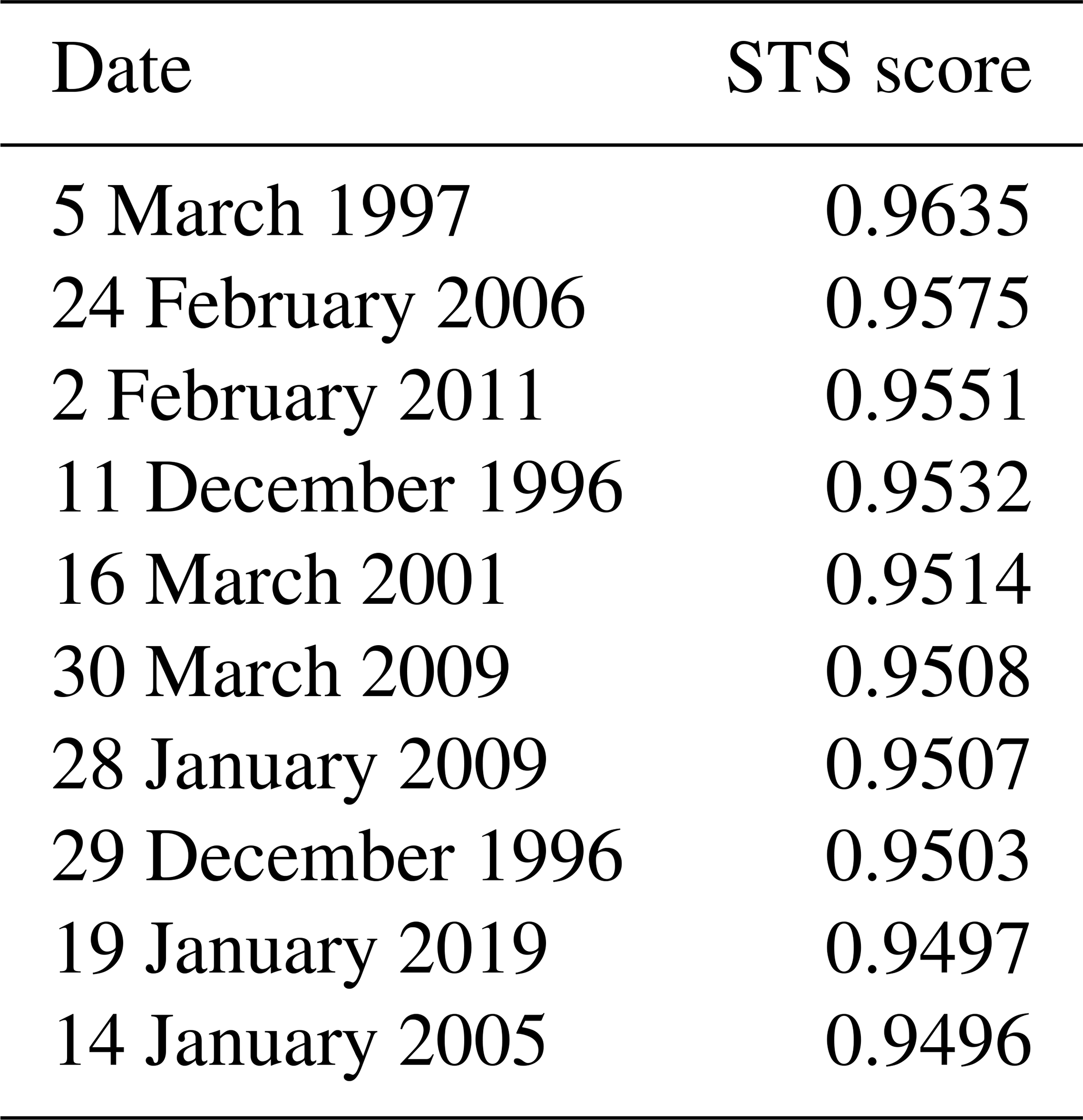
STS: semantic textual similarity.

The results of the comparison are between {0} for the most dissimilar sentences, and {1} if a pair of sentences is very similar (Singhal, 2001). Similar weather conditions were found by ranking all corpora based on their similarity scores (their similarity with the query). We selected only the highest result from the top 10 results of the search process (Table B2). Table B3 presents the weather commentary on the top result of the semantic search.

B2.3 Weather on the selected date

The date with the highest STS scores (5 March 1997) agreed well with the weather features mentioned in the chronicles. The weather on the selected date was generally clear and sunny because of the high-pressure covering Japan's main islands, with the exception of some rain that the chronicles did not mention, demonstrating it may not be possible to observe exactly similar weather. This slight difference may slightly affect the simulated distribution of ashfall.

Figure B6 depicts the weather chart for the chosen date, illustrating more apparent features analogous to the weather chart published during the eruption. The chosen date and the eruption date exhibit the same weather: high-pressure covering all Japan with a low-pressure centred in the north. On the selected date, the high-pressure centre moved from the south to cover Japan at night. The general weather report commentary, accompanied by a daily weather chart, provide critical information that clarified the weather conditions on the respective dates. Another feature, not mentioned in the commentary, was the wind conditions on the selected date. The chronicles reveal that the wind was weak, making it possible to evacuate by boat to escape the eruption (Omori, 1914; Kitagawa, 2015).

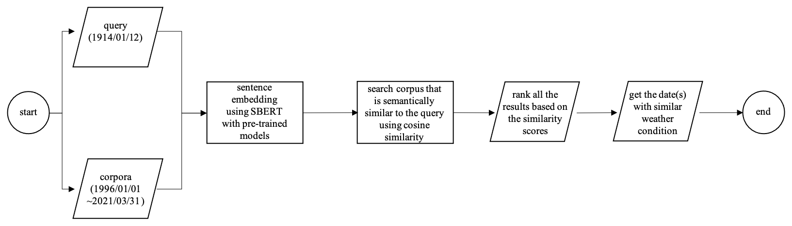
Figure B5 Flowchart for finding dates with weather report commentaries similar to the day of eruption, using a semantic search, based on semantic textual similarity between the old and the modern commentaries, by SentenceBERT (SBERT).

Table B3 Top result of the semantic search with its weather description from the commentary.

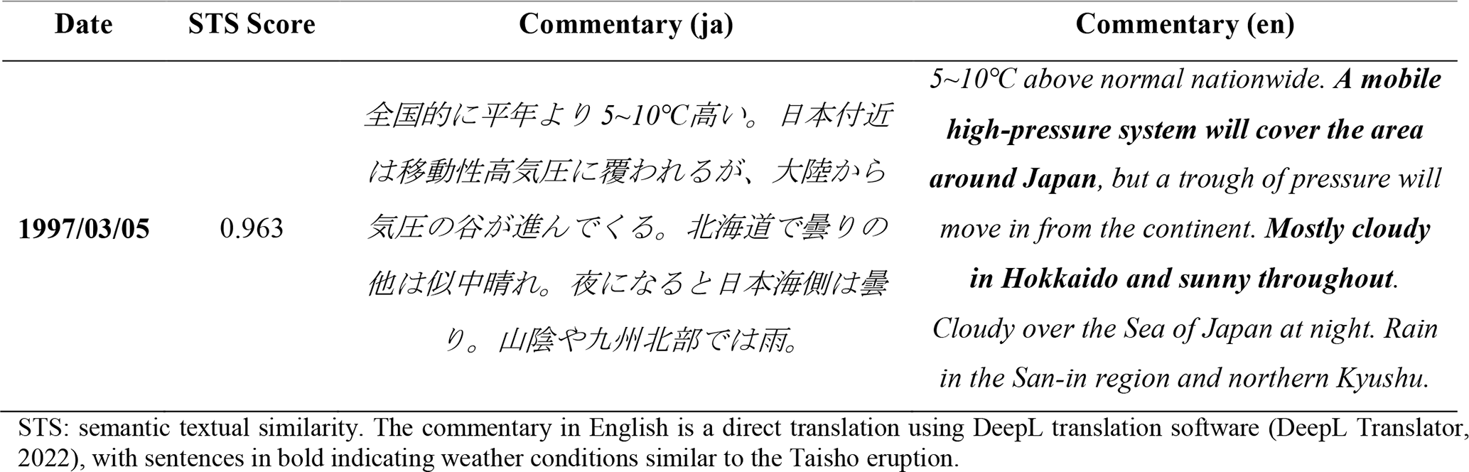
Figure B6 Surface weather chart for Asia Pacific region at 00:00 UTC 5 March 1997. Weather chart image was obtained from the Japan Meteorological Agency (Database of Weather Charts for Hundred Years, 2022; Japan Meteorological Agency, 2022).