Harmonized gap-filled datasets from 20 urban flux tower sites

A total of 20 urban neighbourhood-scale eddy covariance flux tower datasets are made openly available after being harmonized to create a 50 site–year collection with broad diversity in climate and urban surface characteristics. Variables needed as inputs for land surface models (incoming radiation, temperature, humidity, air pressure, wind and precipitation) are quality controlled, gap-filled and prepended with 10 years of reanalysis-derived local data, enabling an extended spin up to equilibrate models with local climate conditions. For both gap filling and spin up, ERA5 reanalysis meteorological data are bias corrected using tower-based observations, accounting for diurnal, seasonal and local urban effects not modelled in ERA5. The bias correction methods developed perform well compared to methods used in other datasets (e.g. WFDE5 or FLUXNET2015). Other variables (turbulent and upwelling radiation fluxes) are harmonized and quality controlled without gap filling. Site description metadata include local land cover fractions (buildings, roads, trees, grass etc.), building height and morphology, aerodynamic roughness estimates, population density and satellite imagery. This open collection can help extend our understanding of urban environmental processes through observational synthesis studies or in the evaluation of land surface environmental models in a wide range of urban settings. These data can be accessed from https://doi.org/10.5281/zenodo.7104984 (Lipson et al., 2022).

1 Background

Tower mounted instruments allow the measurement of land–atmosphere fluxes (e.g. energy, momentum, water, carbon) and local meteorological conditions. These observations are one of the fundamental ways of improving both our understanding and ability to predict biogeophysical and weather-related processes at local scales. Regional and global networks of flux tower sites have helped extend our knowledge of ecosystem and climate science (Novick et al., 2018; Beringer et al., 2016; Yamamoto et al., 2005; Valentini, 2003). Over the last 25 years, networks such as FLUXNET have progressively increased access to flux data through open-source collections (Pastorello et al., 2020), extending the reach and impact of individual site observations through synthesis studies (Baldocchi, 2020) and multi-site environmental modelling and model evaluation projects (Best et al., 2015; Ukkola et al., 2022). However, with few urban sites included, urban areas have not benefited from the improved understanding or more extensive model evaluations that these collections can facilitate.

Urban areas are unique ecosystems, distinct from natural or rural landscapes. First, most people live in cities (UN, 2019) and infrastructure is concentrated within them. Therefore, climate-related health and economic impacts fall disproportionately within urban areas. Second, urban infrastructure (e.g. buildings and roads) along with transient human activities (e.g. energy consumption and irrigation) fundamentally alter surface energy, water and mass exchanges with the atmosphere, modifying local and larger-scale environmental conditions (Oke et al., 2017). Third, as built environments, urban areas are uniquely capable of actively mitigating and adapting to climate change.

Establishing and maintaining long-term flux sites in cities is particularly challenging because of the rarity of appropriate sites with homogenous fetch, the difficulty in gaining approval to access existing towers (e.g. for telecommunications), the cost of constructing tall towers over an aerodynamically rough surface and extremely limited long-term funding opportunities (Arnfield, 2003; Grimmond, 2006; Velasco and Roth, 2010; Feigenwinter et al., 2012; Grimmond and Ward, 2021). Thus, despite the diversity and importance of urban areas across the globe, urban flux tower data are relatively scarce, generally of short duration and rarely open source. Databases identifying urban observational programmes exist (e.g. the Urban Flux Network (Grimmond and Christen, 2012)), however urban flux tower datasets have not previously been brought together into a harmonized, gap-filled, open access collection.

We bring together quality-controlled data from 20 urban sites in an open collection that includes 50 observation years (Lipson et al., 2022). The sites are chosen to be diverse in both regional climates and urban characteristics. As evaluating land surface models is one key application for these data, we create continuous forcing datasets (i.e. with incoming radiation fluxes and other meteorological data) that are gap filled using site specific, bias corrected reanalysis data. Observations are also prepended with 10 years of site-specific reanalysis-derived meteorological data to allow modelled soil moisture and other conditions to equilibrate with local climate conditions during model spin up. These data can be used to drive land surface models offline at a single grid point. Other variables (turbulent and upwelling radiation fluxes) can be used to evaluative models in simulating land–atmosphere energy exchanges, or in observational synthesis studies.

Along with the meteorological data, site characteristics and metadata are provided in a common format. The metadata include tower location, land cover fractions, building heights and morphology, aerodynamic roughness parameter estimates, population density, estimated anthropogenic heat fluxes, site photos and satellite imagery. This collection can help extend our ability to model and understanding of environmental processes in different urban settings.

2 Methods

2.1 Site selection

The initial motivation for collating these flux tower and site data is for use in the Urban-PLUMBER multi-site model evaluation project, currently underway (Lipson, 2021). Urban-PLUMBER draws on methods from the first international urban land surface model comparison (Grimmond et al., 2010, 2011) and the Protocol for the Analysis of Land Surface Models Benchmarking Evaluation Project (PLUMBER (Best et al., 2015)). The latter evaluated land surface models in non-urban (vegetated) areas, while Urban-PLUMBER evaluates land surface models at 20 urban sites (Fig. 1, Table 1).

There is a two-fold use of these observational data in the model evaluation of Urban-PLUMBER:

1. To provide local-scale meteorological input forcing to drive land surface models;

2. To evaluate the performance of models, primarily assessing the local-scale exchange of radiant and turbulent heat fluxes between the surface and lower atmosphere.

With these objectives in mind, the following criteria are used to select flux tower sites:

• appropriately sited for neighbourhood-scale conditions – i.e. within the inertial sub-layer, typically 2–5 times above the average building height and with relatively homogenous fetch (Grimmond, 2006; Barlow, 2014; Grimmond and Ward, 2021);

• requested observations available at 30 or 60 min resolution (Table 2);

• local site characteristics available for description and configuring models;

• a preference for longer datasets (as this allows seasonal and inter-annual variability to be included);

• collectively represent a diverse range of site characteristics and climates.

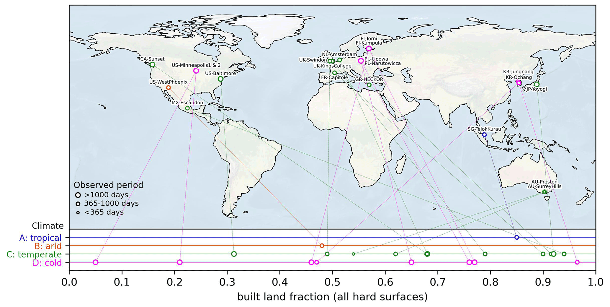
Figure 1 Location of flux tower sites in this collection. Each site Köppen–Geiger climate classification (Beck et al., 2018) and the built land fraction around the tower are indicated at the bottom of the figure.

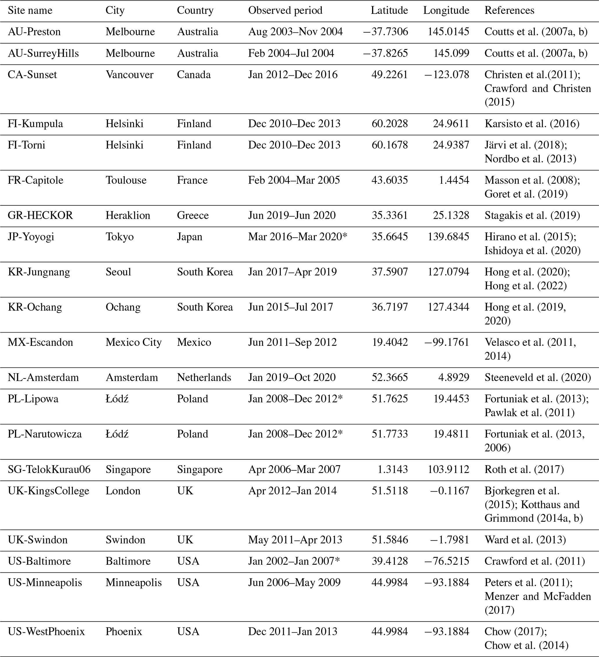
Table 1 Site location and included observation (focus) period. Data providers may have longer observation periods available than are in this collection. Resolution is 30 min (or 60 min if denoted by ^*). All periods in universal time coordinated (UTC). US-Minneapolis data are split based on wind direction and fetch (Sect. 4.5).

Potential sites are identified from published site lists (Grimmond and Christen, 2012; Oke et al., 2017) and open calls for data (e.g. community newsletters (Lipson et al., 2020a), international conferences ((Lipson et al., 2020b, c) and social media professional networks). We deemed 20 sites sufficient for the evaluation project (Table 1), together covering 50 site–years. Included sites have built fractions (i.e. plan area fraction of all impervious surfaces including roofs, roads, other paving etc.) from 0.05 to 0.965, and are located in four major Köppen–Geiger (Beck et al., 2018) climate classes (Fig. 1). Eleven sites are in temperate climates, eight in cold (or continental) climates, and one in each of tropical and arid climates.

Sites are reasonably distributed across mean temperature and precipitation for global urban locations, but gaps remain, particularly in warm, wet and very cold climates (Fig. 2). Some urban flux observations in understudied regions were not included (e.g. Ouagadougou (Offerle et al., 2005), São Paulo (Ferreira et al., 2013), Guangzhou (Shi et al., 2019), Beijing (Dou et al., 2019)) because they do not meet the model evaluation project needs because of the relatively short observed periods for the available data. These regions and climates have large urban populations with significant environmental challenges and have few urban flux tower sites compared with Northern Hemisphere temperate or continental locations (Grimmond, 2006; Roth et al., 2017). Understudied regions and climates should be included in future collections when appropriate time series become available.

Figure 2 Climatology of included sites compared with more than 70 000 global urban areas. Mean temperature and annual precipitation at the 20 tower sites (red, truncated site name, Table 1) from tower observations; global urban locations (grey) from ERA5 surface data (Hersbach et al., 2020, 2018) (2000–2010) from grid nearest to locations identified in the Global Rural–Urban Mapping Project (GRUMP) (Center for International Earth Science Information Network – CIESIN – Columbia University et al., 2017). Locations with rainfall above 3000 mm yr⁻¹ (1.3 % of locations) and mean temperature below −3 ^∘C (0.2  % of locations) are not shown.

2.2 Flux tower data

The observed data are provided in 30 or 60 min periods (Table 1), processed from high-frequency samples by individual observing groups. In the harmonized collection, timestamps are in coordinated universal time (UTC) indicating the end of the measurement period. Variables names and units use ALMA (Assistance for Land-surface Modelling Activities) conventions, a format used in previous land surface model comparisons.

Data are cleaned (Sect. 2.3: Quality control), forcing variables are gap filled (Sect. 2.4) and prepended with data derived from ERA5 (Sect. 2.5), after site-specific corrections (Sect. 2.6). An example of final prepended and gap filled data is shown in Fig. 3 for one site (UK-KingsCollege). Plots for all other variables and sites are also available in the collection (Lipson et al., 2022). Turbulent fluxes and upwelling radiation fluxes are not gap filled (Table 2).

Data are split into forcing and analysis variable sets (Table 2) to allow the forcing variables to be provided to modelling groups as input to run their models. The withheld analysis data are used by the coordinating group to assess the model outputs.

Some additional observed variables (Table 3) have, where practical, been included in the datasets after passing through the quality control steps. Missing forcing variables are obtained using bias corrected reanalysis data (Sect. 2.4). No gap filling is applied to analysis data or additional variables.

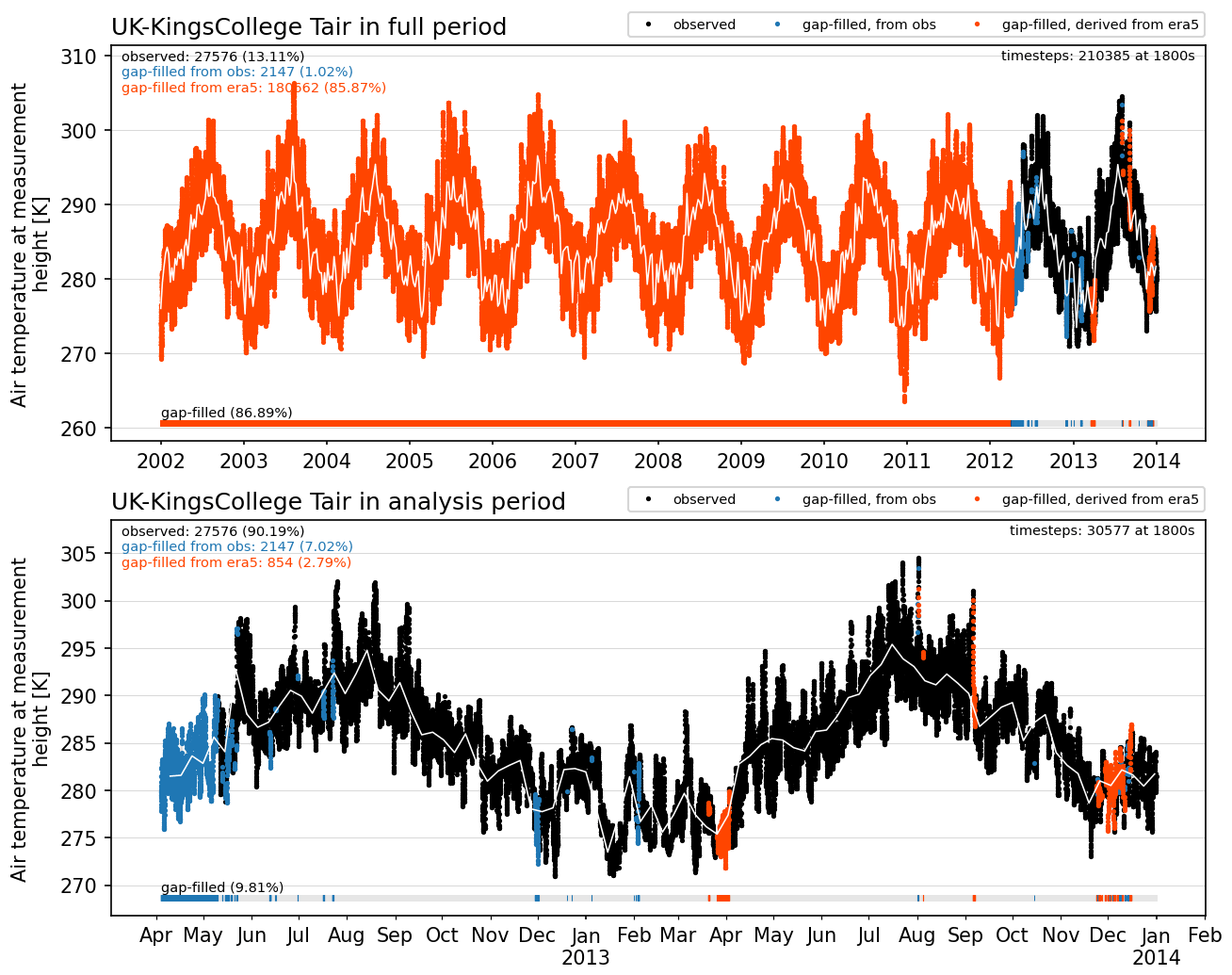
Figure 3 Forcing time series with gap filling. Example shown for air temperature (Tair) at Kings College, London (UK-KingsCollege); (a) full forcing period, including 10 years of ERA5-derived data (red) prior to observations (black) used for model spin up, and (b) focus period used for analysis. Gaps are first filled from nearby tower measurements where available and short gaps (<=2 h) are linearly interpolated (blue). Remaining gaps are filled using the ERA5-derived time series which is seasonally and diurnally bias corrected using site observations. White lines show 7 d mean values. Similar plots are available for other sites within the site data collection (Lipson et al., 2022).

Table 2 Forcing and analysis flux tower data variables. Short name description, units and positive direction use ALMA data conventions. Mean annual estimates of anthropogenic heat flux are included as site metadata. Analysis and additional data are not gap filled. Ground heat flux (Qg) is the heat flux into soil rather than total storage heat flux which is difficult to measure in urban areas (Grimmond and Oke, 1999).

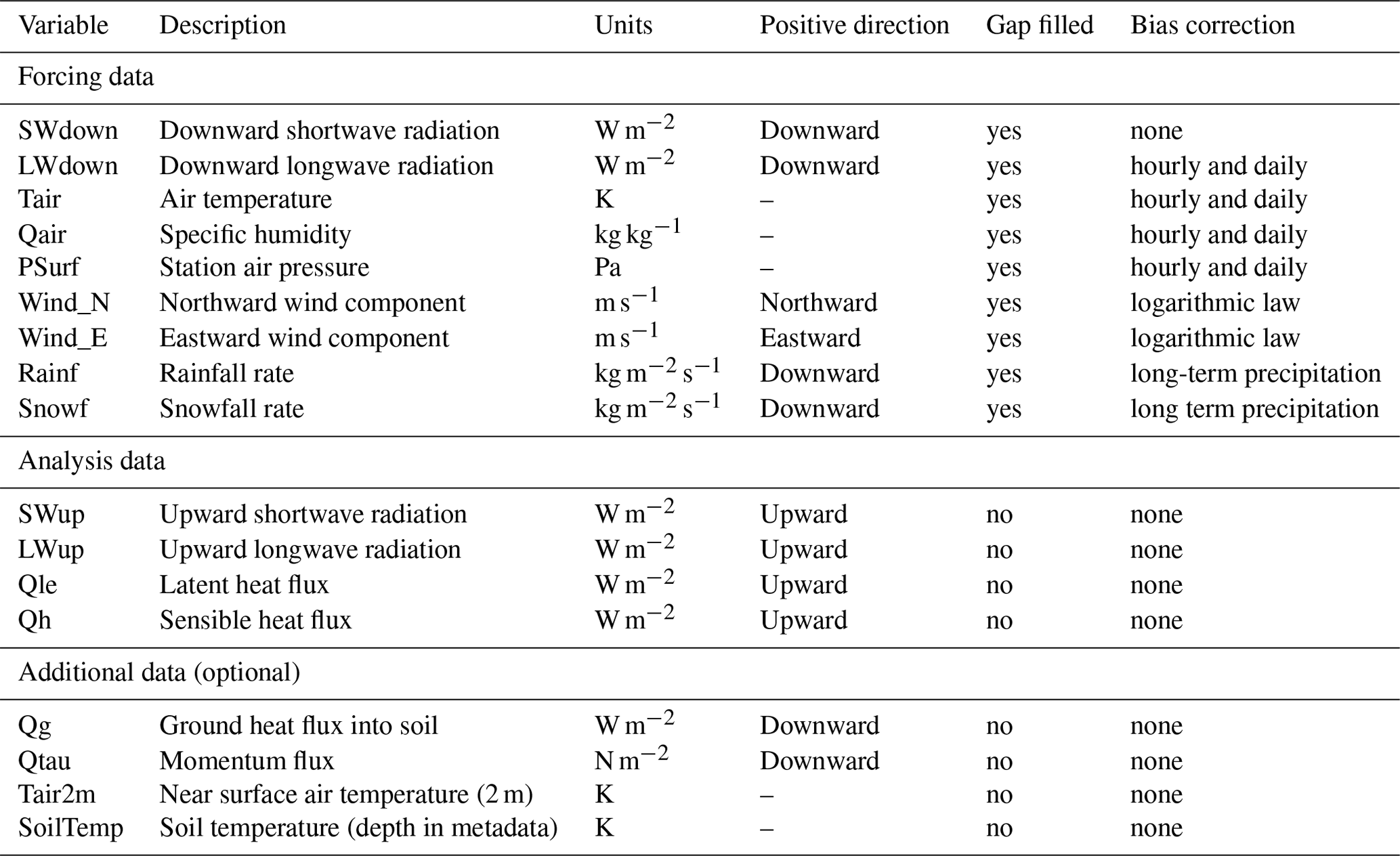
Table 3 Site climate classification missing and additional variables. Climate classification from Köppen–Geiger global dataset (Beck et al., 2018). Table 2 gives variable definitions.

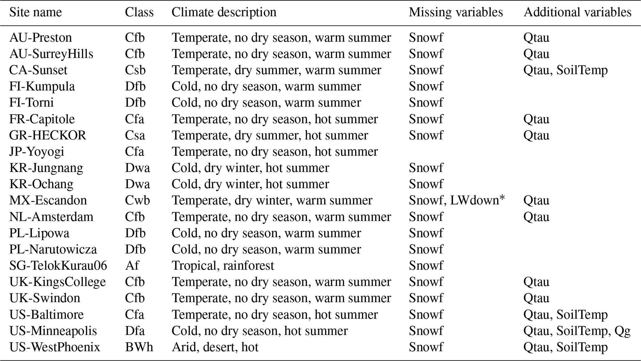
^* Note: as MX-Escandon LWdown data are unavailable during the 2011–2012 focus period, but were available in 2006, this earlier period is used to determine bias correction for ERA5 LWdown data.

2.3 Quality control and assurance

For each site the 30 or 60 min variables are calculated by data providers from high-frequency samples after applying their own quality control measures (e.g. Aubinet et al., 2012; Feigenwinter et al., 2012; Kotthaus and Grimmond, 2012; Vitale et al., 2020). The harmonized collection consists of the data retained after undergoing five additional quality control steps, in the following order:

1. Out-of-range. Removal of unphysical values (e.g. negative shortwave radiation) using the ALMA expected range protocol (Bowling and Polcher, 2001).

2. Night. Nocturnal shortwave radiation set to zero, based on civil twilight (when the sun is 6^∘ below the horizon (Forsythe et al., 1995)).

3. Constant. Four or more time steps with identical values (excluding zero values for shortwave radiation, rainfall and snowfall) are removed as suspicious.

4. Outlier. Values outside ±4 standard deviations for each hour in a rolling 30 d window (to account for diurnal and seasonal variations) removed. Repeat with a larger tolerance (±5 SD, standard deviations) until no outliers remain (Schmid et al., 2000; Vickers and Mahrt, 1997). The outlier test is not applied to precipitation.

5. Visual. Remaining suspect readings are removed manually via visual inspection.

These steps are undertaken in the processing script qc_observations.py (see Sect. 5: Code availability), including periods identified through visual inspection (21 instances across all data). Data removed through quality control are indicated in plots of each variable at each site included in the data collection (Lipson et al., 2022). Note that quality control steps which eliminate observations at particular times (e.g. at night or after rainfall) can introduce biases (Grimmond, 2006). In addition, the outlier check values (step 4) are somewhat arbitrary (as noted in Vickers and Mahrt, 1997). Therefore, we also provide the “raw” observations (prior to quality control discussed here) in the collection as they may be more appropriate for some types of analyses.

Communication, or human errors, also have the potential to degrade or invalidate data (Menard et al., 2021). As part of quality assurance, project coordinators prepared an observational data protocol (Lipson et al., 2021) to explicitly set out requirements for data providers prior to submission of their data. The protocol documented instrument siting requirements, variables and data formats, dataset length and resolution, necessary site characteristic information and metadata, as well as the expectations for data handling, use and authorship. On receiving data, coordinators undertook further checks and identified errors that were not picked up by automated quality control. Identified errors included mislabelled variables and metadata, inconsistent timestamps and unit discrepancies. Many of the errors were identified by comparing provided data with secondary sources such as ERA5, nearby meteorological stations or previous publications. Errors were corrected collaboratively with data providers, some leading to corrections in primary data sources.

2.4 Gap filling

Three gap filling methods are used to create a continuous dataset for forcing variables, in the following order:

• contemporaneous and nearby flux tower or weather observing sites (where available from data providers);

• small gaps (≤2 h) are linearly interpolated from the adjoining observations;

• larger gaps and a 10-year spin up period are filled with bias corrected ERA5 data (Sect. 2.6).

As only one site provided observed snowfall rate (JP-Yoyogi), ERA5 snowfall rates are used for all periods at other sites. At those sites the additional water equivalent from ERA5 snowfall is removed from subsequent observed rainfall until mass balance of observed total precipitation is achieved. This corrects melting snow being recorded as rainfall.

2.5 ERA5 reanalysis data

The ERA5 reanalysis product (Hersbach et al., 2020) assimilates global satellite, atmospheric and ground-based observations to constrain numerical weather prediction simulations, producing global output at 0.25^∘ spatial and hourly temporal resolutions from 1959 to the present. It is therefore useful as a globally consistent and accessible source of meteorological data across space and time. ERA5, and its lower resolution predecessor ERA-Interim (Dee et al., 2011), have been used extensively to provide meteorological forcing data to drive land surface models and gap fill flux tower observations (Vuichard and Papale, 2015; Kokkonen et al., 2018; Pastorello et al., 2020; Ukkola et al., 2017, 2022).

The ERA5 hourly single level (Hersbach et al., 2018) dataset (retrieved from NCI Australia (Druken, 2020)) is used for gap filling missing observations within the focus periods (Table 1) and for the 10-year model spin up period. However, combining ERA5 data directly with urban flux tower observations has several deficiencies.

Grid-scale ERA5 data are not directly compatible with point-scale urban flux tower observations. This incompatibility is three-fold:

1. Horizontally. The ERA5 grid cell area (of the order of 500 km²) does not match the flux footprint from tower observations (of order 1 km²). The ERA5 surface characteristics, including elevation, are based on an average description for the grid which may differ from surface characteristics around the observing tower, particularly in coastal or mountainous regions (Martens et al., 2020) in which many cities are located.

2. Vertically. ERA5 provide near-surface variables (2 or 10 m above ground level), aligning with World Meteorological Organization (WMO) guidelines for standard regional observations taken over short grass (World Meteorological Organization, 2008). As the urban roughness elements (e.g. buildings) are much taller than grass, instruments are mounted on towers at heights greater than 2–5 times average building height in order to be located within the inertial sub layer or constant flux layer (Velasco and Roth, 2010; Barlow, 2014; Grimmond and Ward, 2021).

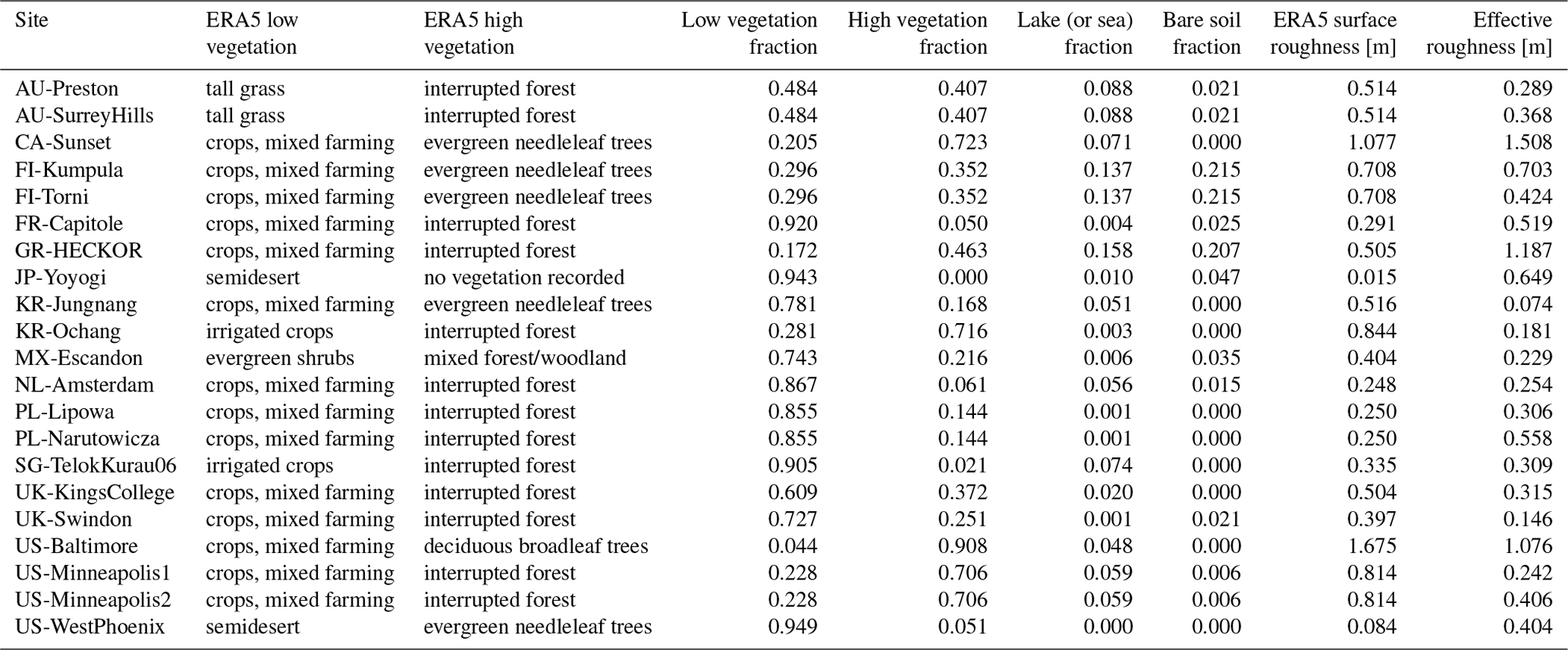
3. Land surface. As the current operational ERA5 modelling systems do not include an urban land surface scheme (Boussetta et al., 2013; McNorton et al., 2021), other land types (grass, crops, shrubs, trees etc.) are used to characterize the grid cell (Table 4). Urban land surfaces are well known to alter local meteorological conditions (Oke et al., 2017), therefore ERA5 output will likely differ from locally observed conditions.

Outside of cities there are known diurnal and seasonal biases between the ERA5 near-surface variables and observations (Haiden et al., 2018; Betts et al., 2019; Nogueira, 2020; Martens et al., 2020; Jiang et al., 2021). These biases are an outcome of simplifying assumptions made in model parameterizations and inadequacies of modelling frameworks in general (Cucchi et al., 2020). Various approaches to reduce ERA5 biases in non-urban areas have been proposed. For example, the Water and Global Change (WATCH) Forcing Data (WFD) project use gridded observations to bias correct ERA-Interim data (Weedon et al., 2011), and more recently ERA5 data, creating the global WFDE5 dataset for impact studies (Cucchi et al., 2020). WFDE5 relies on the Climate Research Unit (CRU) monthly time series of gridded observations with resolution courser than ERA5 (New et al., 1999), requiring ERA5 to be regridded to a lower resolution. This may reduce the representativeness of the ERA5 data, particularly in heterogenous or complex terrain.

Alternatively, local observations can be used to bias correct ERA data, e.g. the linear regression corrections using tower observations applied to FLUXNET datasets (Vuichard and Papale, 2015; Pastorello et al., 2020). However, linear methods neither conserve the variability of observations (Vuichard and Papale, 2015) (Sect. 3), nor can they correct diurnal timing differences within ERA5 data (e.g. out of phase from urban temporal profiles, which are typically delayed compared with non-urban surfaces used in ERA5, Fig. 4).

To account for the mischaracterization of sites (Table 4) and other listed deficiencies in ERA5, we develop a novel set of methods to bias correct ERA5 data to better represent observed urban conditions (Sect. 2.6).

Table 4 Surface cover information as specified in ERA5 differs from actual tower site characteristics (see Table 6), and so ERA5 data are corrected (Sect. 2.6). Given the ERA5 surface roughness values vary slightly through time, the values listed are indicative (from 1 January 2000). Effective roughness is our correction accounting for observed urban mean wind speeds.

2.6 Bias correction methods

Bias correction approaches used in the collection depend on the forcing variable (Table 2) and are described below.

2.7 Hourly and daily corrections

For incoming longwave radiation, air temperature, specific humidity and air pressure, the mean bias between ERA5 and local flux tower observations are calculated for each hour (h) and each day of a year (D) in a 60 d rolling window of a representative year (Fig. 4a). The calculated bias η_bias(D, h) is subtracted from the complete ERA5 time series η_ERA5(t) to create a new corrected time series:

$$\begin{array}{}\text{(1)}& \mathit{\eta }\left(t\right)={\mathit{\eta }}_{\mathrm{ERA}\mathrm{5}}\left(t\right)-{\mathit{\eta }}_{\mathrm{bias}}\left(D,h\right).\end{array}$$

The ERA5 data are from the grid nearest the observation site with at least 50 % land. The resulting corrected time series (e.g. Fig. 4b) is used for gap filling site observations and for the spin up period. The subroutine rolling_hourly_bias_correction in the file pipeline_functions.py (Sect. 5) undertakes corrections with the following steps:

1. If observations have a 30 min resolution, average to 60 min to match ERA5 periods;

2. Remove ERA5 data for time periods where site observations are missing;

3. Calculate mean for each hour with both data sets to create a “representative” year of 366 d;

4. Extend to a 3-year period by duplication to provide smoother transitions at year end;

5. Calculate hourly means in a 60 d rolling window across the repeating time series, excluding data in windows with less than 30 observations. Repeat mean calculation for greater smoothing;

6. Calculate a time series of the bias between observed and ERA5 rolling means;

7. Fill gaps in the bias time series by linear interpolation through each hour separately;

8. Remove first and last year in the bias time series, using only the central year to bias correct each hour in the original ERA5 time series.

A 60 d rolling window is selected to smooth out individual weather events while still capturing seasonal variation. Repeating the representative year three times prior to smoothing ensures bias corrections match at the start and end of the year. The resulting set of bias correction curves (Fig. 4a) has greater robustness when multiple years are available.

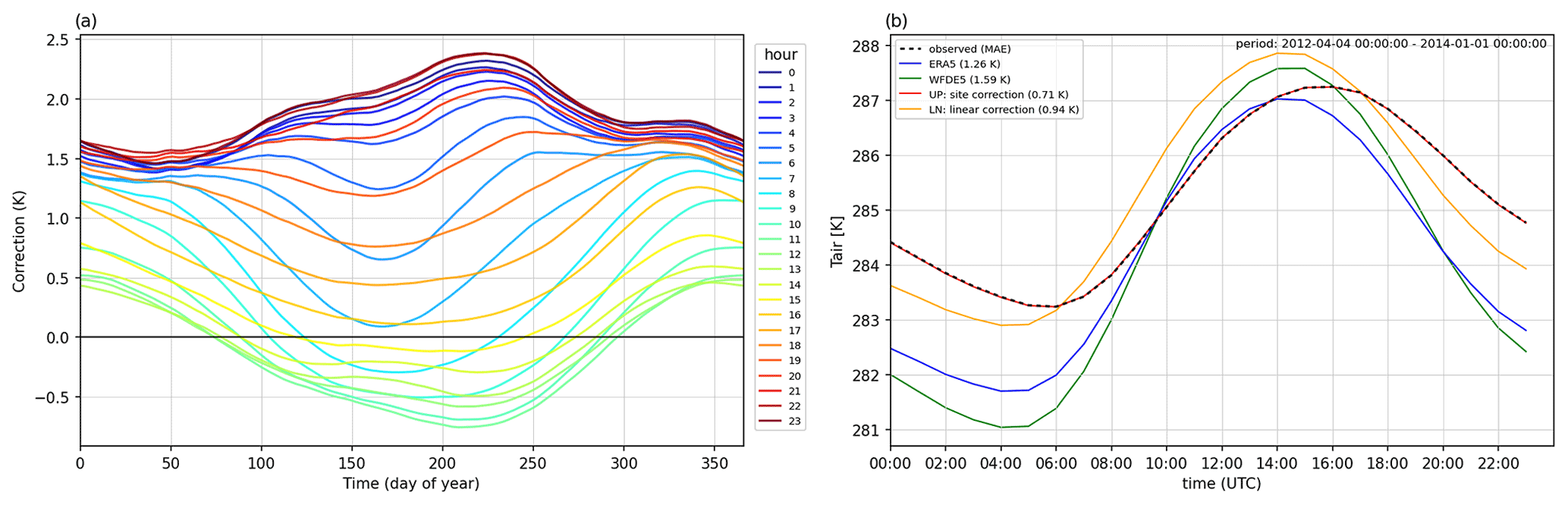
Figure 4 Urban-PLUMBER reanalysis bias correction methods. Demonstrated using air temperature (Tair) for the grid containing the King's College London site (UK-KingsCollege). (a) Hourly (colour) bias calculated for each day of a “representative” year and applied to entire ERA5 time series; (b) diurnal hourly mean Urban-PLUMBER correction (UP, red), observations (black), original ERA5 data (blue), WFDE5 bias corrected data (green) and linear bias correction method used in FLUXNET (LN, yellow). Our new UP method has smaller mean absolute errors (MAE) overall, and can correct both pattern and phase errors of ERA5 (Sect. 3).

2.7.1 Logarithmic wind profile correction

Wind speed differences between ERA5 and site observations can result from errors in modelled synoptic-scale speeds, differences in representative heights, and differences in surface aerodynamic properties like roughness and displacement height. To correct bias and maintain standard deviations of the wind components (U, V) of observations at sensor height (z_site), the following correction to ERA5 data is undertaken assuming both a logarithmic wind profile and neutral conditions (Goret et al., 2019):

$$\begin{array}{}\text{(2)}& u_{\mathrm{corr}}=u_{\mathrm{ERA}\mathrm{5}}{\displaystyle \frac{\ln \left(\frac{z_{\mathrm{site}}-d_{\mathrm{site}}}{z_{\mathrm{0},\mathrm{site}}}\right)}{\ln \left(\frac{z_{\mathrm{grid}}-d_{\mathrm{grid}}}{z_{\mathrm{0},\mathrm{grid}}}\right)}},\end{array}$$

where u_corr is the corrected wind speed at z_site. The ERA5 wind (u_ERA5) at 10 m (z_grid) is used with the site surface roughness (z_0,site) and displacement height (d_site), and grid roughness (z_0,grid) (Table 4) while assuming grid displacement height (d_grid) is zero for simplicity. If the resulting mean value of u_corr differs from observed mean value by more than 0.01 m s⁻¹, then z_0,grid is iteratively adapted until this threshold accuracy in mean wind speed is achieved. Derived z_0,grid values are given in Table 4 (last column). Note this approach ignores seasonal effects from vegetation phenology and directional effects but ensures mean wind speeds are appropriate at the urban z_site while conserving variability within the ERA5 derived wind data.

2.7.2 Long-term precipitation correction

Total precipitation is an important variable in urban land surface models because of the effect on soil moisture which evolves over multi-year periods (Best and Grimmond, 2014). Most of the observational datasets included are not long enough to capture interannual variations. We therefore use longer term total precipitation (P) from nearby stations from the Global Historical Climatology Network – Daily (GHCND) (Menne et al., 2012) over a 10 year period to correct ERA5 rain and snow fluxes (ϕ) at each time step:

$$\begin{array}{}\text{(3)}& {\mathit{\varphi }}_{\mathrm{corr}}={\displaystyle \frac{{\sum }_{i=\mathrm{1}}^{\mathrm{10}\mathrm{yrs}}{P}_{\mathrm{GHCND}}}{{\sum }_{i=\mathrm{1}}^{\mathrm{10}\mathrm{yrs}}{P}_{\mathrm{ERA}\mathrm{5}}}}{\mathit{\varphi }}_{\mathrm{ERA}\mathrm{5}}\left(t\right).\end{array}$$

Gaps in the nearest GHCND station data are progressively filled by the next nearest station until no gaps are present. If gaps could not be filled with GHNCD stations within 2^∘ of latitude and longitude from the flux tower, and no alternative records are found (e.g. from national meteorological and hydrological services), then ERA5 rates are used unadjusted (viz., KR-Ochang and KR-Jungnang). This assumes precipitation occurs on the same dates and at the same times in ERA5 and observed datasets, which may become less valid under increasingly convective conditions.

2.7.3 Linear bias correction

The FLUXNET2015 collection of 212 flux tower sites (Pastorello et al., 2020) bias correction method uses linear regression between site observations and reanalysis data to derive one slope (s) and intercept (b) per site, hence “unbiasing” all ERA time steps (i):

$$\begin{array}{}\text{(4)}& {\mathrm{LN}}_i=s\cdot \mathrm{ERA}{\mathrm{5}}_i+b.\end{array}$$

Following FLUXNET2015, global radiation and wind fields are assigned an intercept of zero, and precipitation is not linearly modified (Vuichard and Papale, 2015). FLUXNET2015 uses the coarser resolution ERA-Interim (spatial: 0.5^∘ cf. 0.25^∘; temporal 3 h cf. 1 h) than ERA5. In this evaluation we use ERA5, which is found to be a consistent improvement over ERA-Interim (Albergel et al., 2018). However, after assessment we chose not to use a linear method (LN) for correcting variables in this collection. Its description is retained here for comparison purposes (Sect. 3).

3 Gap filling evaluation

Site observations are quality controlled by individual data providers and collectively for this project (Sect. 2.3). The observed data required for forcing land surface models are then gap filled using a novel method of bias correcting reanalysis data. In this section, four methods which draw on ERA5 data are evaluated:

1. ERA5. Nearest land-based 0.25^∘ resolution ERA5 (Hersbach et al., 2018) grid without bias correction.

2. W5. Nearest WFDE5 (Cucchi et al., 2020) grid (which uses bias correction from 0.5 ^∘ CRU monthly gridded observations).

3. UP. The Urban-PLUMBER methods described here (using site observations for bias correction).

4. LN. Linear methods based on FLUXNET2015 (Vuichard and Papale, 2015; Pastorello et al., 2020) (using site observations for bias correction).

To evaluate the methods available for gap filling, quality-controlled tower site observations (O_i) are used to assess the calculated value (η) at timestep i using three metrics:

• a.

  Mean bias error (MBE): $\frac{{\sum }_{i=\mathrm{1}}^n{\mathit{\eta }}_i-O_i}{n}$

• b.

  Mean absolute error (MAE): $\frac{{\sum }_{i=\mathrm{1}}^n\left|{\mathit{\eta }}_i-O_i\right|}{n}$

• c.

  Normalized standard deviation (nSD): $\sqrt{{\frac{{\sum }_{i=\mathrm{1}}^n\left({\mathit{\eta }}_i-\stackrel{\mathrm{‾}}{\mathit{\eta }}\right)}{n-\mathrm{1}}}^{\mathrm{2}}}/\sqrt{{\frac{{\sum }_{i=\mathrm{1}}^n\left(O_i-\stackrel{\mathrm{‾}}{O}\right)}{n-\mathrm{1}}}^{\mathrm{2}}}$.

Where $\stackrel{\mathrm{‾}}{O}$ and $\stackrel{\mathrm{‾}}{\mathit{\eta }}$ are time-averaged over n data points. The timestamps for each variable are made consistent between the data sources: ERA5 are hourly time ending or instantaneous data (Hersbach et al., 2018); 60 min site observations are hour ending; 30 min site observations are converted to 60 min time ending by averaging; whereas as the WFDE5 SWdown, LWdown and Rainf are natively 60 min time beginning (Cucchi et al., 2020), they are shifted forward to match the time ending timestamps; and WFDE5 Tair, Qair, Psurf and Wind are instantaneous samples on the hour so their timestamp remains unchanged.

To summarize each metric for the 20 sites, we use boxplots (Fig. 5) for the seven forcing variables. The evaluation inherently considers the net differences associated with both the spatial (vertical and surface cover) differences and errors (model and observation) from the two datasets. Uncorrected ERA5 (blue, Fig. 5) biases are generally negative for Tair, LWdown and Wind, and generally positive for Qair and SWdown. These biases can be partly explained by the ERA5 framework not including an urban surface model. For example, the well-documented warmer air temperature in cities (urban heat island) are not modelled in ERA5 because natural land surfaces are assumed in simulations (Table 4), although ERA5 can include an urban signal if the data assimilated are from within urban areas (Tang et al., 2021). Qair shows a general positive bias as evapotranspiration will be overestimated in ERA5 without an urban land surface representation. Likewise, ERA5 SWdown are overestimated and LWdown underestimated possibly because urban air pollution effects are not included (Oke, 1988).

Other discrepancies between ERA5 data and site data arise from elevation differences in height above sea level (a.s.l.) of the ERA5 grid and site. For example, the MX-Escandon tower in Mexico City measurement height is 2277 m a.s.l., whereas the ERA5 grid cell is assigned a surface elevation of 2540 m a.s.l. because the cell includes nearby mountains. This 263 m difference causes a negative bias to Psurf of 2594 Pa and contributes to a Tair difference of −2.15 K. Additionally, orographic uplift increases the grid cell rainfall, leading to positive ERA5 bias of 2.25 × 10⁻⁵ kg m⁻² s⁻¹ (+710 mm yr⁻¹) compared with the MX-Escandon site observations. The ERA5 rainfall bias is even more pronounced at CA-Sunset in Vancouver, Canada, with a +1178 mm yr⁻¹ bias. These results are consistent with other studies highlighting discrepancies between reanalysis and local data in mountainous regions (Kokkonen et al., 2018).

The other three methods (WFDE5 (W5), linear debiasing (LN) and the Urban-PLUMBER corrections (UP)) apply bias corrections to ERA5 data, and so may be expected to reduce ERA5 errors. However, W5 does not reduce errors at these sites, most likely because the observations used for W5 bias correction are at very different spatial scales to the flux tower footprints (2500 km² versus 1 km²) and include observations from non-urban locations. The LN and UP methods eliminate spatial mismatches by drawing on local site or nearby rain gauge observations. As such, they do reduce the mean bias error to near zero for most variables. Notably, the UP methods outperform LN methods in normalized standard deviation. As Vuichard and Papale (2015) noted, linear methods do not conserve the variability of observations, nor can they correct for diurnal phase shifts of some variables observed in urban areas (Fig. 4). Therefore, we consider the UP methods to be the most appropriate at these urban sites. However, we apply no bias corrections to SWdown because the hourly and daily corrections (i.e. UP methods applied to other variables) adversely impact the standard deviation errors, as does the LN method for SWdown.

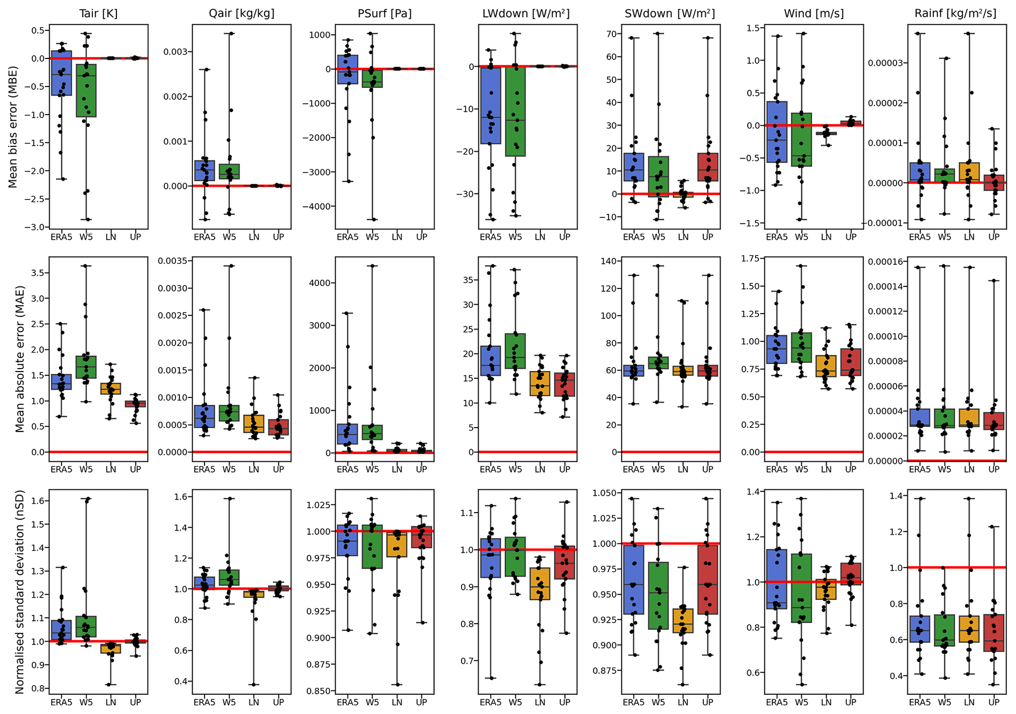
Figure 5 Evaluation of bias correction methods. Four methods (colour) to create gap filled observed time series data: ERA5 (blue), WFDE5 (W5, green), linear debiasing (LN, orange), UP (red, this study) using (row 1) mean bias error, (row 2) mean absolute error, (row 3) normalized standard deviation, with the 20 individual sites (dots), and ideal agreement with observations (red line) and boxplot showing distribution. The UP corrections (selected for use in this study) have lower overall errors (cf. other methods) except SWdown, where no corrections to ERA5 are applied.

4 Data availability

Data described in this manuscript can be accessed from https://doi.org/10.5281/zenodo.7104984 (Lipson et al., 2022) under a Creative Commons Attribution licence (CC-BY-4.0).

We recommend data users consult with site contributing authors and/or the coordination team early (i.e. planning stage) in projects that plan to use these data. Relevant contacts are included in site metadata.

5 Code availability

Code used to process datasets are available at https://doi.org/10.5281/zenodo.7108466 (Lipson, 2022a).

Code used to create paper figures are available at https://doi.org/10.5281/zenodo.6590941 (Lipson, 2022b).

6 Data records

6.1 Data format

Time series data and site descriptive metadata are recorded in both plain text and netCDF4 (Rew et al., 1989) formats. Each site folder contains the following time series:

• [sitename]_raw_observations_[version]: site observed before project-wide quality control and gap filling (Table 1 gives period)

• [sitename]_clean_observations_[version]: after project-wide quality control and gap filling (Table 1 gives period)

• [sitename]_metforcing_[version]: continuous observations with reanalysis-derived data after quality control and gap filling (Table 2; forcing data for 10-year spin up, then Table 1 periods)

• [sitename]_era5_corrected_[version]: continuous time series (1990–2020) of bias corrected ERA5 reanalysis meteorological data (as used for gap filling and prepending metforcing observations).

Each site folder also contains the following site metadata:

• [sitename]_sitedata_[version].csv: comma separated text file for site characteristics metadata e.g. latitude, longitude, surface cover fraction and morphology (Tables 5, 6). This site characteristic data are also included within the metforcing netcdf (for convenience)

• index.html: a summary page of site information in html format, including site characteristics, site images, time series, gap filling, quality control and diurnal plots.

6.2 Time series metadata

The time series files include the following metadata:

• title: short description of the file

• summary: longer description of the file

• sitename: site code (e.g. AU-Preston)

• long_sitename: site long name, including city and country information

• version: version of current file

• time_coverage_start: start of time series in UTC (includes spin up) with period ending timestamps

• time_coverage_end: end of time series in UTC with period ending timestamps

• time_analysis_start: start of observed (focus) period in UTC with period ending timestamps

• time_shown_in: time standard (always UTC)

• local_utc_offset_hours: offset in hours of local time from UTC

• timestep_interval_seconds: period of block averaging in seconds (time step)

• timestep_number_spinup: number of time steps prior to observed focus period

• timestep_number_analysis: number of time steps in observed focus period

• project_contact: contact details for the Urban-PLUMBER project coordinators

• observations_contact: contact details of the observational site data providers

• observations_reference: published references associated with the observations

• date_created: date and time of creation of this file

• source: repository for processing code

• comment: additional comments associated with this dataset (e.g. excluded wind sectors).

Text file time series include metadata headers indicated with a hash (#) at line beginnings. Columns are headed by variable names in ALMA format (Table 2). NetCDF4 files include identical data, with additional attributes for each variable:

• long_name: plain language description of variable

• standard_name: equivalent variable name under the CF (climate and forecast) conventions

• units: SI (international system) units

• ancillary_variables: name of the associated quality control flag variable.

NetCDF files also include site characteristics parameter values and descriptions (Table 5). Times in all datasets are UTC. Python programmes are provided (Lipson, 2022a) to convert UTC times to local standard time (convert_UTC_to_local_time.py), and netCDF to text (convert_nc_to_text.py).

Table 5 Site characteristic metadata description and units. Parameters are determined for the turbulent flux footprint extent (Table 6), except 1–4 which are applicable to the tower itself, and 19 which is a function of the radiometer field of view (Offerle et al., 2003) and differs from the turbulent flux footprint (Schmid et al., 1991).

6.3 Site characteristics metadata

Site characteristics (Tables 5, 6) are essential for any use of these data, and fundamental to application of land surface models. These metadata are provided in two machine readable forms (plain text in csv files and netCDF4). The metadata are primarily drawn from published sources or as advised by the data providers. If local parameters are not known, values are estimated from high-resolution global datasets or derived from empirical relations. The sources for each parameter are included within the site characteristic metadata.

There are numerous methods to estimate the probable extent and weighting of turbulent fluxes footprints relative to the eddy covariance sensors located on a flux tower (Velasco and Roth, 2010). The eddy covariance flux footprint provides a basis to identify which area (and weighting) should be used to estimate the land surface fractions impacting the measurements. Some studies in this collection determine the footprint and resulting land cover fractions dynamically (e.g. for each 30 min period based on that period's observed atmospheric variables such as stability and wind direction), whereas others used a constant radius (e.g. based on the footprint climatology or rule of thumb) (Table 6). Standardizing the method to determine land cover fractions across sites is beyond the scope of this work, so users of metadata should be mindful of these differences.

Different methods for estimating surface roughness length and zero-plane displacement height can give significantly different values (Kent et al., 2017). Given that different data providers have derived values using different methods, we also provide values using two consistent morphometric methods (Macdonald (Macdonald et al., 1998) and Kanda (Kanda et al., 2013); Table 5, parameters 26–29) derived from surface fraction and building height parameters within the measurement footprint (Table 6). The Kanda modification to the Macdonald method accounts for the variability in roughness element height, resulting in larger displacement heights which are closer to estimates made with anemometric methods (Kent et al., 2017). The Macdonald method assumes that all the buildings have the same average roughness element height. However, care must be taken when using Kanda values as some urban land surface models expect displacement height to be always lower than average building height (Hertwig et al., 2020).

Where not known, building height standard deviation (σ_H) is estimated from an empirical relation to building mean height (H_ave) (Kanda et al., 2013):

$$\begin{array}{}\text{(5)}& {\mathit{\sigma }}_{\mathrm{H}}=\mathrm{1.05}{H}_{\mathrm{ave}}-\mathrm{3.7}.\end{array}$$

Similarly, unknown local wall to plan area ratios (λ_w) are derived from roof area fraction (λ_p) and canyon height to width ratio ($H/W$) assuming an infinite canyon geometry (Masson et al., 2020):

$$\begin{array}{}\text{(6)}& {\mathit{\lambda }}_{\mathrm{w}}=\mathrm{2}\left(\mathrm{1}-{\mathit{\lambda }}_{\mathrm{p}}\right)H/W.\end{array}$$

Frontal area index (λ_f) is sometimes reported in site literature without $H/W$ or λ_w, in which case these are estimated (again assuming an infinite canyon geometry) with (Porson et al., 2010):

$$\begin{array}{}\text{(7)}& {\mathit{\lambda }}_{\mathrm{f}}={\displaystyle \frac{\mathrm{2}}{\mathit{\pi }}}\left(\mathrm{1}-{\mathit{\lambda }}_{\mathrm{p}}\right)H/W.\end{array}$$

Where not known or provided, mean annual anthropogenic heat flux (Varquez et al., 2021) or soil characteristics (Hengl, 2018a, b, c) are estimated from global datasets at 1 km or lower resolutions.

Table 6 Select site characteristic values (see Table 5 for definitions). Other site characteristic values and sources are provided within the collection (Lipson et al., 2022). Areas analysed for land cover fractions and roughness parameters are based on either a static radius around the flux tower (value given) or a dynamic footprint model (fpm). For the latter, the spatial extents are the order of a few hundred metres but are dynamic varying for example with atmospheric stability and wind direction (Grimmond and Ward, 2021).

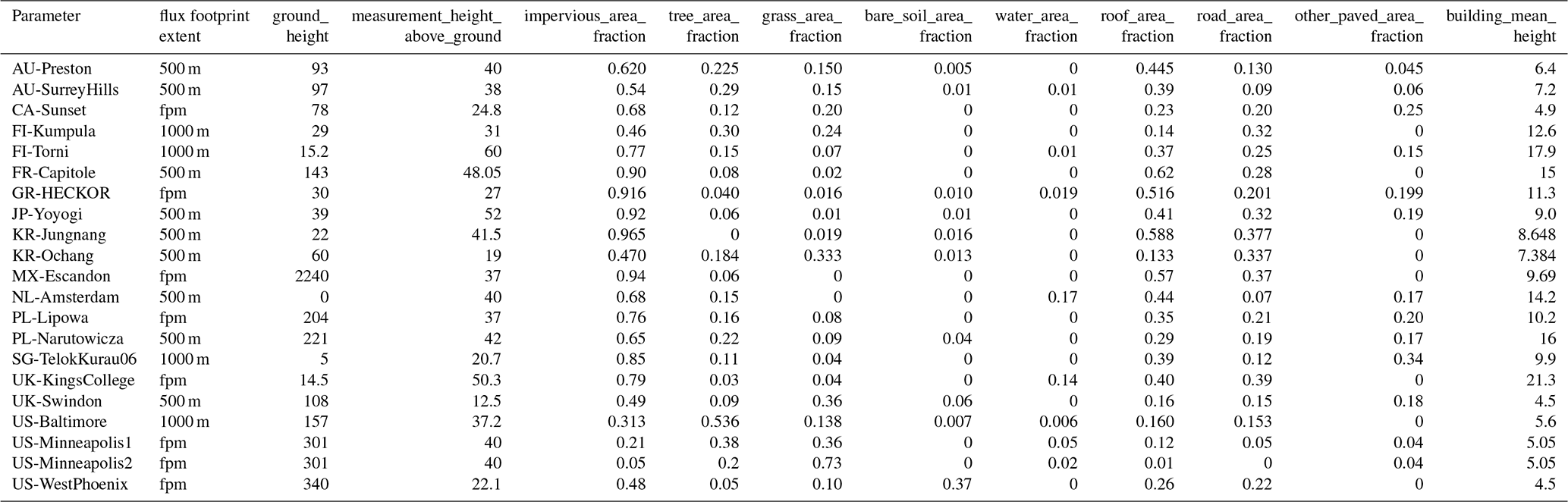
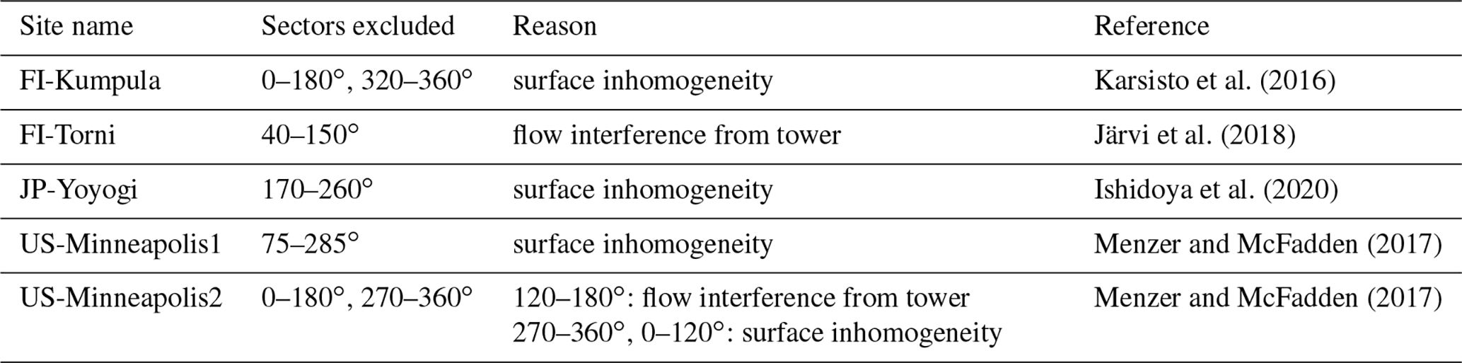
Table 7 Site wind sector exclusions. Sites with sensible and latent heat fluxes excluded because of land cover or land use differences by wind sectors as described in the reference provided. Maps of these sectors are provided in the site data collection (Lipson et al., 2022).

Table 8 Funding acknowledgements for individual sites.

6.4 Data flags

Each variable for each time step has a quality control (qc) flag. For example, LWdown_qc lists qc flags for LWdown at each time step. Flag numbers are consistent across all variables:

• 0.

  observed by measurement at site and passes project quality control tests

• 1.

  filled by observation; interpolated from site observations over short (2 h) periods OR filled by observations from nearby (<10 km) stations over longer periods

• 2.

  filled by ERA5; derived from ERA5 with site specific bias correction

• 3.

  missing or removed through quality control (occurs only in time series without gap filling).

6.5 Wind sector exclusions

Turbulent flux data are excluded from certain wind directions (Table 7) because of

• interference on flow from tower structure (as identified by data providers);

• markedly different land cover characteristics from sectors of interest (with guidance from data providers).

The US-Minneapolis site has different surface cover by wind direction but is retained in the collection because of both a long observation period and its distinct land cover characteristics. Following previous studies (Menzer and McFadden, 2017) we subdivide these data into low density residential area (northern sectors, US-Minneapolis2) and irrigated grassland with few built structures (south, US-Minneapolis1). Each are given their own site time series and metadata, resulting in 21 datasets.