the Creative Commons Attribution 4.0 License.
the Creative Commons Attribution 4.0 License.
 | 04 Nov 2022
Mesoscale observations of temperature and salinity in the Arctic Transpolar Drift: a high-resolution dataset from the MOSAiC Distributed Network
Ivan Kuznetsov
Ying-Chih Fang
Benjamin Rabe
Measurements targeting mesoscale and smaller-scale processes in the ice-covered part of the Arctic Ocean are sparse in all seasons. As a result, there are significant knowledge gaps with respect to these processes, particularly related to the role of eddies and fronts in the coupled ocean–atmosphere–sea ice system. Here we present a unique observational dataset of upper ocean temperature and salinity collected by a set of buoys installed on ice floes as part of the Multidisciplinary drifting Observatory for the Study of Arctic Climate (MOSAiC) Distributed Network. The multi-sensor systems, each equipped with five temperature and salinity recorders on a 100 m long inductive modem tether, drifted together with the main MOSAiC ice camp through the Arctic Transpolar Drift between October 2019 and August 2020. They transmitted hydrographic in situ data via the iridium satellite network at 10 min intervals. While three buoys failed early due to ice dynamics, five of them recorded data continuously for 10 months. A total of four units were successfully recovered in early August 2020, additionally yielding internally stored instrument data at 2 min intervals. The raw data were merged, processed, quality controlled, and validated using independent measurements also obtained during MOSAiC. Compilations of the raw and processed datasets are publicly available at https://doi.org/10.1594/PANGAEA.937271 (Hoppmann et al., 2021i) and https://doi.org/10.1594/PANGAEA.940320 (Hoppmann et al., 2022i), respectively. As an important part of the MOSAiC physical oceanography program, this unique dataset has many synergies with the manifold co-located observational datasets and is expected to yield significant insights into ocean processes and to contribute to the validation of high-resolution numerical simulations. While this dataset has the potential to contribute to submesoscale process studies, this paper mainly highlights selected preliminary findings on mesoscale processes.
- Article
(9466 KB) - Full-text XML
- BibTeX
- EndNote


Oceanic mesoscales host a variety of important features and processes that have been extensively studied during the past 4 decades, pioneered by the Mid-Ocean Dynamics Experiment in the 1970s (MODE, Bretherton et al., 1976; Jochum and Murtugudde, 2006; McWilliams, 1976). Mesoscale processes are characterized by horizontal scales of a few to several tens of kilometers and temporal scales much greater than the local inertial periods, up to the order of 1 month. An important consequence is that the vertical velocities are 103 to 104 times weaker than the horizontal velocities (Thomas et al., 2008). The mesoscales are the major contributors in terms of the kinetic energy reservoir (Ferrari and Wunsch, 2008) and usually manifest in the form of geostrophic eddies that are shown ubiquitously in present-day satellite imagery (McGillicuddy, 2016). Their occurrence has been linked to concurrently occurring tilted isopycnals (Gill et al., 1974), where baroclinic instabilities submesoscale release potential energy which generates eddies. Global estimates of mesoscale eddy variability indicate that mesoscale eddies can be correlated with the first-mode baroclinic Rossby radius (Chelton et al., 1998; Smith, 2007). In the Arctic Ocean, recent studies have highlighted the role of mesoscale eddies and the significant fraction that eddy kinetic energy contributes to total kinetic energy in observations (Zhao et al., 2014) and high-resolution numerical simulations (Wang et al., 2020). At the same time, eddies have likely been historically underestimated in key regions of the Arctic Ocean (Porter et al., 2020).
Apart from the mesoscales, recent advancements in instrumentation and computing power have allowed us to further appreciate the submesoscale regime which resides between the mesoscale and turbulence (McWilliams, 2016). Submesoscales are characterized by O(1) Rossby and Richardson numbers and evolve with relative shorter spatial O(100 m to 10 km) and temporal O(d) scales. Mesoscale and submesoscale processes both feature non-negligible vertical velocities (D'Asaro et al., 2011; Thomas et al., 2008) that make them unique in bridging the momentum exchange between the ocean surface layer and the interior underneath (e.g., Lévy et al., 2018). Numerical simulations have shown that shifts from mesoscale to submesoscale regimes (Capet et al., 2008) result in frontal instabilities (e.g., Mahadevan, 2016; Mahadevan et al., 2010) and secondary ageostrophic circulation (Thomas, 2005). In the Arctic basin, mesoscale and submesoscale variability does not only occur under seasonal ice cover and in the marginal ice zone (MIZ; e.g., Gallaher et al., 2016) but also under perennial sea ice. Although eddy activity is lower in the central Arctic than near the boundaries, the portion of total kinetic energy due to mesoscale eddies (eddy kinetic energy) is significant in the central Arctic Ocean (Zhao et al., 2014; Wang et al., 2020; von Appen et al., 2022). The local processes acting at the mesoscale and smaller scales not only alter the local hydrography and circulation but also feed back to the large scale. State-of-the-art climate and Earth system models would benefit from advancing our knowledge of these processes and improving parameterization (Hewitt et al., 2020).
Although present-day field campaigns may be able to observe mesoscale currents and features by remote sensing at lower latitudes (Gaube et al., 2015) and as part of carefully planned synoptic surveys (Huang et al., 2018), high latitudes pose a greater challenge. In the Arctic basin, mesoscales shrink to an order of 5 to 20 km (Nurser and Bacon, 2014; D'Asaro, 1988; Manley and Hunkins, 1985) from those of 50 to 100 km at mid-latitudes (e.g., Smith, 2007). Observations of the mesoscale by remote sensing are limited in the central Arctic by seasonal and perennial ice cover, though plans for dedicated satellite missions exist to cover even the submesoscale (e.g., Gommenginger et al., 2019). Ship-based surveys in the central Arctic Ocean can give a good impression of the large-scale state and interannual changes. However, observations of mesoscale processes remain a challenge due to the scales involved and the typically synoptic design of hydrographic surveys. In addition, they are limited by logistical constraints and the high cost of operation in the pack ice to the melting season and early freeze-up from about June to September. Furthermore, towed or autonomous platforms, such as autonomous underwater vehicles (AUVs) or gliders, remain difficult or impossible to operate in the central Arctic ice pack. Similar constraints apply to seafloor moorings (e.g., Zhao et al., 2016).
One way to overcome these constraints is the use of ice-tethered drifting ocean-observing platforms. During the past 3 decades, these have increasingly facilitated in situ observations to augment ship-based surveys. Examples include the Polar Ocean Profiling System (POPS; Kikuchi et al., 2007), the Ice-Tethered Profiler (ITP; Toole et al., 2006), and the Ice–Atmosphere–Ocean Observing System (IAOOS) platforms (Koenig et al., 2016; Athanase et al., 2019). Providing year-round time series in the Transpolar Drift and the Canada Basin, they are usually aimed at large-scale monitoring, with efforts such as the Marginal Ice Zone program in the Canada Basin (Lee et al., 2017) being the exception. Coordinated efforts particularly aim at vertically connecting the processes in the realms of the atmosphere, sea ice, and ocean. However, most deployments are not aimed at resolving the mesoscale in the horizontal. Several systems have contained components that were designed to measure temperature and salinity at a high frequency to capture short-term fluctuations, such as those associated with submesoscale, mesoscale and internal wave variability. Examples are again the Woods Hole Oceanographic Institution (WHOI) ITP (Toole et al., 2006), the Japan Marine Science and Technology Center (JAMSTEC) Compact Arctic Drifter buoys (J-CAD; Hatakeyama et al., 2012), and the UpTempO (Steele, 2017) and WARM buoys (Hill et al., 2019) .
The details of mesoscale processes and their effect on water mass formation, local circulation, and fluxes need to be known to understand changes on an Arctic-wide scale, particularly with respect to the variety of feedbacks between the ocean and the sea ice and the atmosphere (e.g., Zhao et al., 2016). The current lack of knowledge and incorrect representation of vertical mixing processes in climate models result in large biases in Arctic Ocean temperature and salinity (Ilicak et al., 2016) and limit our knowledge of their effect on large-scale circulation (Timmermans and Marshall, 2020). The magnitude of the mesoscale (e.g., Nurser and Bacon, 2014; Zhao et al., 2014) indicates the potential to detect associated ocean features with novel, autonomous in situ platforms, given the quasi-synoptic character of observations from drifting sea ice.
Here we present a unique observational dataset from the central Arctic Ocean obtained as part of the physical oceanography work program during the Multidisciplinary Drifting Observatory for the Study of Arctic Climate (MOSAiC) experiment in 2019/2020 (Rabe et al., 2022). We designed and deployed an autonomous buoy array equipped with several oceanographic sensors upstream in the significantly understudied albeit crucially important Arctic Transpolar Drift that can resolve processes on the mesoscale over a full seasonal cycle. Below we outline the concept, realization, data processing, and data validation. We discuss environmental, technical, and analytical challenges. We present exemplary results to showcase the potential for an analysis of mesoscale variability and conclude with an outlook on the wider scope of this unique dataset, including the potential use for the study of submesoscale processes such as the restratification or internal waves.
2.1 General concept
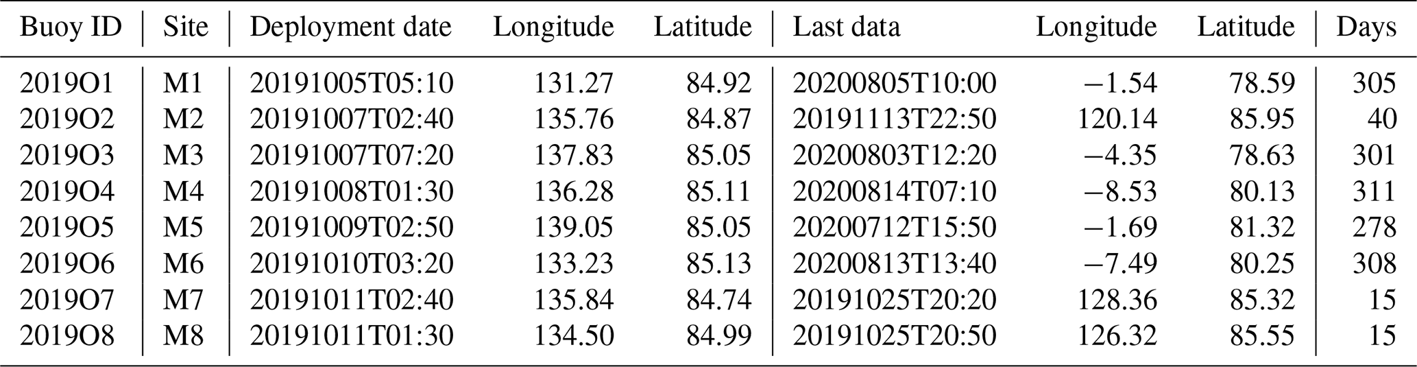
To address some of the knowledge gaps outlined above, a set of eight buoys carrying a suite of oceanographic sensors was deployed upstream in the Transpolar Drift in October 2019 as part of the MOSAiC Distributed Network (DN). The instruments were installed within ∼ 40 km of the German research icebreaker R/V Polarstern, which was planned to stay anchored to the same ice floe for an entire year and constituted the main MOSAiC ice camp (also referred to as the Central Observatory). Incorporating a diverse collection of autonomous instrumentation, the DN was intended to spatially extend and complement the extensive work program conducted by the different teams (Nicolaus et al., 2022; Shupe et al., 2022; Rabe et al., 2022) in the Central Observatory and to bridge the gap between the spot measurements and larger-scale airborne and satellite observations. The DN consisted of several complex instrument systems distributed to a dozen main sites, complemented by a large number of additional simple GPS buoys in the wider DN. Of these sites, eight were equipped with the buoys presented in this study and were each co-deployed with a handful of other instruments (see below). This distribution, together with the ice drift, covered the mesoscale (of the order of a few tens of kilometers) and, to some extent, the submesoscale (of the order of 1 km). While we were originally aiming for less spacing between the individual buoys to better resolve the submesoscale processes, the challenging ice conditions and absence of sufficiently stable floes required us to change the plan and extend the deployment area to reduce the risk of early failures. The exceptionally dynamic ice pack in winter 2019/2020 led to a failure of several other buoys in the early period of MOSAiC (including three of eight units described here; see Sect. 2.3).
Our focus was on the upper water column and, in particular, the whole upper ocean mixed layer across most of the Eurasian Basin. The primary aim of the expedition was to capture local processes in the strongly stratified region of the Transpolar Drift, which features near-surface waters that are much fresher and colder than those found in the Nansen Basin close to the inflow of water of Atlantic origin. The drift started in the Amundsen Basin, as close to the Siberian shelves as possible, where the Transpolar Drift stream originates. That allowed a continuous drift into late spring without relocating the ice camp and with a chance to recover the buoys. Placing instruments in the upper 100 m was expected to capture processes in the seasonally deepening and subsequently restratifying mixed layer and to also cover part of the upper halocline throughout much of the year.
We required a sufficient number of measurement points in the vertical to give a good indication of the structure of the mixed layer and the upper halocline. This especially aimed at resolving passing eddies or fronts, while minimizing the number of sensor packages and associated costs. Deployment alongside ocean profilers at different sites within the DN, such as the Woods Hole Ice-Tethered Profiler (Toole et al., 2006) or the Drift-Towing Ocean Profiler (DTOP; Ocean University of China, 2021), ensured that the vertical structure of the upper water column was measured to 1 dbar resolution at least once a day. At the same time, our systems aimed at capturing transient phenomena, such as internal waves or eddies, requiring measurements as frequent as 2 min.
2.2 Instrument description
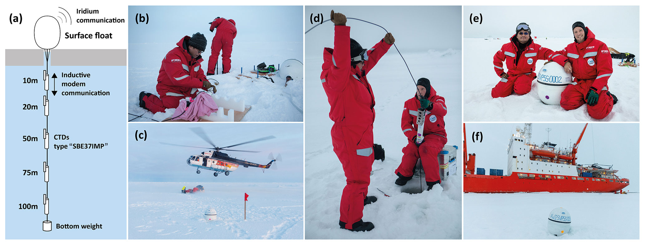
The sensor platform, hereafter referred to as Salinity Ice Tether (SIT), is a floatable buoy built by Pacific Gyre (California, USA) and comprised an oval surface float that housed the main electronics and batteries, connected to a 100 m long inductive modem cable with a 10 kg terminal weight attached to the bottom (Fig. 1a). Along this tether, five SBE37IMP MicroCAT CTD (conductivity–temperature–depth) instruments built by Sea-Bird Scientific, California, USA, and hereafter referred to as CTDs, were mounted at depths of 10, 20, 50, 75, and 100 m. Following the naming convention of the general AWI (Alfred-Wegener-Institut) buoy program, which was also implemented for all MOSAiC buoys, we identify the individual buoys with an ID consisting of the deployment year (in this case, 2019), followed by a buoy-type-specific letter (in this case, O) and a running number (from 1 to 8). The corresponding buoy IDs are 2019O1 to 2019O8 for the eight SIT systems. Furthermore, we refer to the individual CTDs by the buoy ID and the nominal CTD deployment depth, i.e., 2019O1-10m is the CTD attached to the tether of buoy 2019O1 at a nominal depth of 10 m.
To ensure an operational time of ∼ 1 year, the individual CTDs were set to record data internally at 2 min intervals, independent of the buoys' own sample and transmit intervals. The surface buoy itself recorded the GPS position and surface temperature and carried a submergence sensor. Furthermore, the buoy controller polled all CTDs for an additional measurement according to a preconfigured buoy sampling interval, which could, in principle, be adjusted by sending a reconfiguration command via iridium if necessary. However, throughout our experiment, all buoys were set to take a measurement and immediately transmit the corresponding data at a fixed 10 min interval, which was chosen to ensure an operational time of the surface buoy of at least 1 year. In summary, the internal sampling interval of the CTDs was 2 min, while an additional CTD measurement was obtained and transmitted by the buoy every 10 min together with the corresponding auxiliary (meta)data.
Upon removal of a magnet at the side of the hull after deployment, the buoy was switched on and automatically activated the internal 2 min sampling of the attached CTDs. The buoy controller sampled all of the CTDs 1 min before a scheduled transmission. After reading the auxiliary sensors, the buoy controller sampled the GPS at the scheduled transmit time to obtain a valid GPS position for transmission. The data resulting from this measurement cycle were then compressed into a file and sent via the iridium short-burst data (sbd) protocol to a shore-based server, which decoded the data and provided the data for download. In the standard buoy firmware, pressure is by default rounded to 0.1 dbar before transmission to save on data size and transmission costs. Unfortunately, this could not be changed during operation. Salinity was calculated on the server side based on the transmitted temperature, conductivity, and pressure measurements according to the Practical Salinity Scale 1978 (PSS-78). For the final dataset, however, practical salinity was recalculated from these variables using the MATLAB Gibbs–SeaWater (GSW) Toolbox version 3.05.5 (McDougall and Barker, 2011).
The SBE37 MicroCAT CTD itself (either in its normal configuration or inductive modem configuration) is a reliable and accurate sensor that has been used for studies of physical oceanography on various platforms all over the world for decades, particularly for moored operations (e.g., Beszczynska-Möller et al., 2012). The stated initial accuracy for this sensor type is ±0.003 mS cm−1 for conductivity, ±0.002 ∘C for temperature, and ±0.1 % of the full-scale range for pressure. For our instruments, the pressure rating was between 100 and 1000 m due to the limited availability of 100 m pressure sensors at the time of manufacturing. The initial accuracy for a 100 m calibrated pressure sensor (0.1 % of the full-scale range) is thereby ∼ 0.1 dbar. As stated earlier, the buoy firmware only transmitted 10 min pressure records to the first decimal, resulting in a vertical resolution of 0.1 dbar compared to 0.02 to 0.002 dbar (0.002 % full-scale range) of the CTDs themselves. Since the accuracy is of the same order of magnitude, we do not consider the transmission limitation for pressure as being significant in relation to our final dataset. For datasets that include the internally recorded data of the recovered CTDs, the pressure records as sent by the buoy have been interpolated to improve their quality (see Sect. 3). The typical sensor stability is rated as 0.003 mS cm−1 and 0.0002 ∘C per month for conductivity and temperature, respectively, and 0.05 % of the full-scale range (pressure) per year.
2.3 Field deployment and recovery
The buoys were deployed along with a suite of other platforms during the set-up phase of the MOSAiC Distributed Network by the Russian icebreaker Akademik Fedorov in early October 2019 (Fig. 1b–f). A few days before reaching the deployment destination, the instruments were successfully tested on the deck. Ice floes were selected based on an inspection of high-resolution satellite imagery and helicopter surveys. The ice conditions were challenging for permanent installations since thin ice was predominant in the deployment area (Krumpen et al., 2020). The station work was either done from the ship or by Mi-8 helicopters. The instruments were co-installed on selected ice floes together with SIMBA-type ice mass balance buoys (Jackson et al., 2013), snow buoys (Nicolaus et al., 2021a), and DTOPs.
The snow buoy, SIMBA, and SIT buoys were installed close to each other, while the DTOP was installed at a distance of at least 70 m away. After a deployment site with sufficiently stable level ice was chosen, the buoy tether was laid out on the ice, and the CTDs were attached to their designated depth positions along the cable. The instruments were covered with towels for protection during handling on the ice and snow. The cable and instruments were manually lowered into the ocean through a 25 cm diameter hole in the ice, and the surface float was placed on top of the hole. Air temperatures were as low as −15 ∘C. Table 1 summarizes the deployment information for each instrument.
The trajectories of the buoys during their 10-month-long drift are presented in Sect. 4.2. Buoys 2019O2, 2019O7, and 2019O8 failed within the first 5 weeks after their deployment. Buoy 2019O5 failed in July 2020, most likely due to ice ridging, having survived for 9 months. The other four buoys were recovered from the decaying ice field in the marginal ice zone of Fram Strait in August 2020 by the German and Russian icebreakers R/V Polarstern and Akademik Tryoshnikov.
In this paper, we exclusively refer to in situ temperature (T in ∘C; ITS-90) and practical salinity (S, unitless; PSS-78) if not stated otherwise. The final data collection consists of eight individual datasets, with one for each buoy. Of these, four are merged products of the initial iridium-transmitted buoy data (10 min interval) and the corresponding CTD data from recovered instruments (2 min interval). To ensure the highest possible data quality, and at the same time giving the end-user the possibility to apply his/her own quality checks, we decided to not entirely remove questionable data but instead apply a primary quality flagging scheme to the oceanographic data in a modified version of the scheme proposed in UNESCO-IOC (2013). The primary-level flagging scheme we use here is composed of five quality values which are defined as follows: 1 – good, 2 – modified, 3 – questionable, 4 – bad, and 9 – missing data. The difference from the originally proposed scheme is that “2 – not evaluated” was replaced by “2 – modified”, as we think it should be general practice to evaluate all data points. In some cases, as also described below, the quality of the data could be improved by the modification of the original record, which is indicated by the “2 – modified” flag. We applied this scheme to the oceanographic data only. We decided against using an additional, secondary flagging scheme, as further discrimination of the quality checks described below would not provide any substantial added value to our data.
Each dataset was compiled in the following way: first, the buoy data were obtained from the Pacific Gyre web server. A handful of obvious GPS outliers were removed, and the gaps were filled by linear interpolation. Buoy drift speed was calculated from the difference between adjacent GPS positions. The resulting drift speeds were consistent throughout, and no further processing was applied. Surface temperature data were controlled for plausibility mainly by a general range check, and no correction was necessary. The polled sampling of the CTDs was initiated by the buoy 1 min before the acquisition of GPS position and time. For consistency and simplicity, we used the time of the CTD sampling as the general timestamp (rather than the GPS fix 1 min later), thus accepting an additional uncertainty in the GPS position of <30 m, depending on the drift speed. If higher temporal resolution CTD data were available for a particular buoy, then both datasets were merged (see below). No quality flags for position or surface temperature are given since their quality is overall good, and the oceanographic measurements are the focus of this observational dataset. Data from the 20 recovered CTDs (corresponding buoy IDs of 2019O1, 2019O3, 2019O4, and 2019O6) were downloaded using the SeatermV2 software (version 2.8.0.119) by Sea-Bird Scientific. For logistical reasons, data from 2019O1 and 2019O3 were downloaded at sea as .cap files, whereas data from 2019O4 and 2019O6 were recovered at home after the end of MOSAiC as standard .hex, .xml, and .xmlcon files and converted to .cnv files using the Sea-Bird Scientific software SBE Data Processing (version 7.26.7).
The CTD timestamps were checked for consistency using distinct features in the pressure records of each set of CTDs installed on any given buoy (for example, when all instruments were lifted at the same time due to an increased drift speed as a result of strong winds). 2019O4-75m was mistakenly configured to a 30 s measurement interval, which led to an early power failure (see below). For this CTD, only every fourth record was used for the final dataset for consistency reasons. The full dataset is, however, still available in the raw data archive. Also, the instrument time of 2019O4-75m had an offset of 56 s, which was corrected.
For the four merged data products, the data were combined and reordered based on their timestamps. All records before the deployment have been removed from the dataset (not flagged), based on the pressure record of the instruments. In some instances, the initial conductivity values appeared suspiciously low, sometimes even with sudden jumps to higher values. There is a high probability that these are erroneous records caused by ice formation in the pump or conductivity cell. This could have been caused by the instrument being exposed to cold air temperatures before deployment through the ice. In most instances, this effect disappeared after a few days to several weeks. We tried to identify a point in the time series where the salinity data start to become reasonable (for example, after the last suspicious jump) by conducting plausibility checks and comparing against adjacent CTDs or comparing to other buoy data, and we flagged all prior records as “3 – questionable”. Temperature and pressure records were not affected by this. While the latter were generally clean and reliable, as expected from these sensors, conductivity measurements sometimes exhibited suspicious values that were potentially caused by particles in the cells. Conductivity values below 20 and above 40 mS cm−1 were flagged as “4 – bad”; most of the time, this coincided with the conductivity issue outlined above. For the five longest time series (∼ 10 months), a moving average filter was tested and tuned to identify the outliers that still fell within the allowed global range. No suitable window size was found that would exclusively catch the outliers, so we decided to rather flag the remaining suspicious records manually as “3 – questionable”. Furthermore, 2019O3-10m exhibited a small, but suspicious, conductivity drop, which was several days long, from 34.1 to 33.5 in June 2020 that was not accompanied by a change in temperature and thereby subsequently flagged as “3 – questionable”.
Buoy 2019O6 exhibited more outliers than the other buoy datasets. Since these outliers were not found on the recovered CTDs themselves, we conclude that this was caused by an issue in the inductive modem communication rather than by a problem with the CTD sensor measurement. Since these outliers were too numerous for manual flagging, a moving average filter (window size 14) was applied to determine and flag these records as “3 – questionable” (∼ 1000 total records for 2019O6). The few remaining outliers (<20) were manually flagged. Interestingly, in some instances, this inductive modem issue resulted in records being wrongly assigned, i.e., a measurement taken by 2019O6-10m was assigned by the buoy to 2019O6-20m. In these cases, the records were reassigned and flagged as “2 – modified”. Buoy 2019O6's temperature and pressure suffered the same problem. The temperature was checked using subsequent moving average filters (window sizes 14 and 11; ∼ 1900 outliers flagged as “3 – questionable”), and the remaining few outliers were manually flagged as either “3 – questionable” or “2 – modified”.
When CTD data were available, the 0.1 dbar and 10 min resolution buoy pressure records were linearly interpolated in time using the CTD pressure records to achieve a consistent pressure time series. The interpolated records were flagged as “2 – modified” accordingly. This procedure also removed the pressure outliers caused by the inductive modem issue from the 2019O6 record, so no additional filtering was necessary. Each CTD record for a given buoy was assigned a GPS position by the linear interpolation of the corresponding buoy GPS record, and drift speed was recalculated accordingly. Instrument depth was calculated from clean pressure readings and latitude using the MATLAB GSW toolbox function gsw_z_from_p (McDougall and Barker, 2011).
Although practical salinity was initially calculated and provided on the server side, we recalculated this variable from conductivity, temperature, and pressure according to the PSS-78 algorithm (MATLAB GSW toolbox function gsw_SP_from_C). Quality flags for calculated depths and salinities were inherited from T, C, and p. Finally, salinity was despiked using a moving average filter with a window size of 12 (equivalent to between 20 and 120 min), depending on whether the dataset contained 2 min or 10 min data. The final (<120) outliers identified by this filter were flagged as “3 – questionable”. An overview of the processing and flagging procedure is given in Fig. 2.
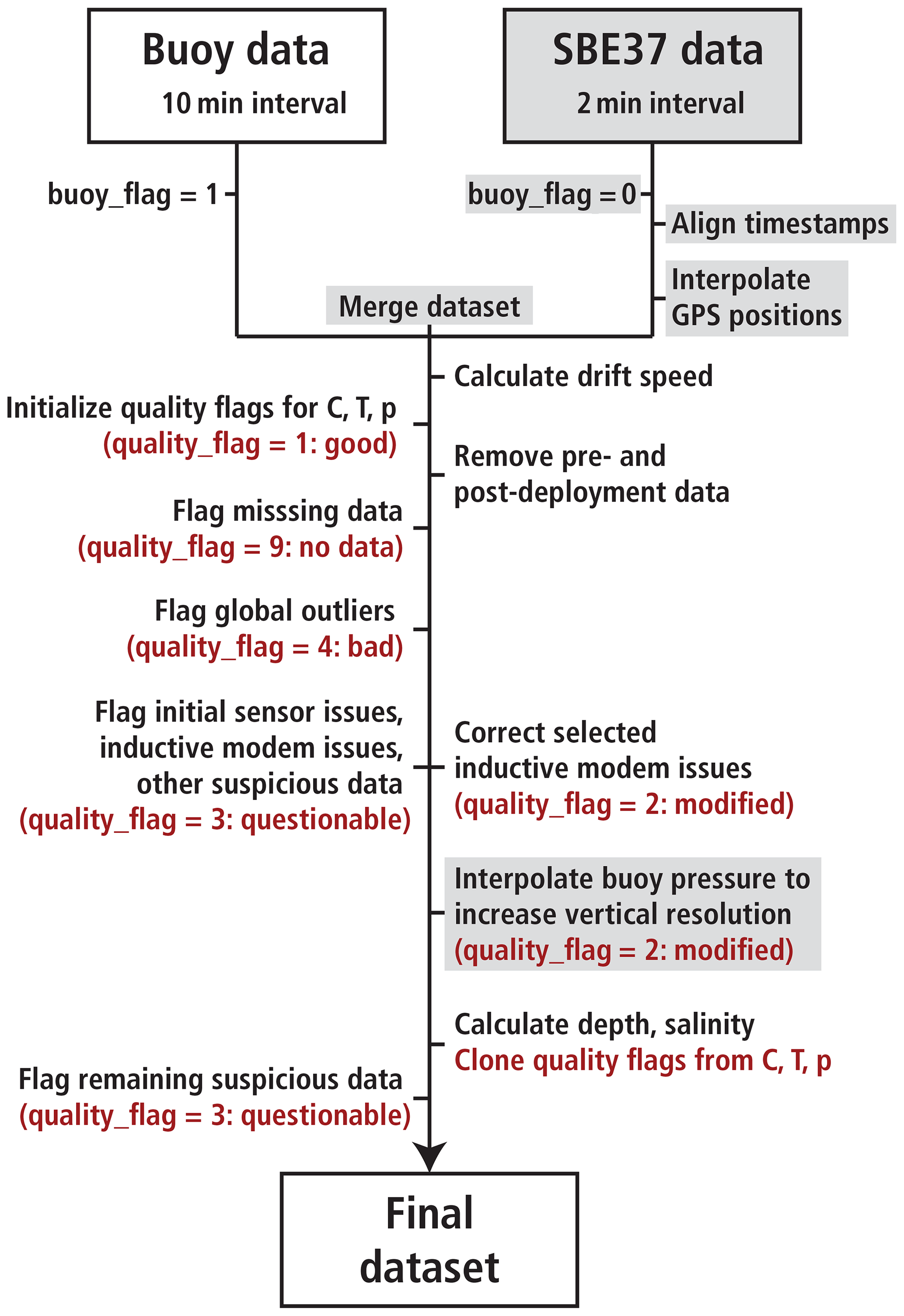
Figure 2Schematic outlining the individual steps of data processing and quality control using primary flags (indicated in red) according to a slightly modified version of UNESCO-IOC (2013). The additional processing steps required when merging buoy and recovered CTD data are indicated in gray. Procedures to the left of the processing arrow represent flagging without modification of the original data, whereas processing steps to the right involve removal and modification of original data or calculation of secondary parameters.
4.1 Dataset description
The processing described above yielded eight individual time series, with one for each buoy. Only three time series (2019O2, 2019O7, and 2019O8) comprise a few weeks, while five (2019O1, 2019O3, 2019O4, 2019O5, and 2019O6) are ∼ 10 months long. For 2019O1, 2019O3, 2019O4, and 2019O6, we supply a merged product that combines buoy and CTD data, while for 2019O2, 2019O5, 2019O7, and 2019O8, only the transmitted buoy records are available.
Table 2Variables of the processed dataset. The nominal depths of the five CTDs (represented by gear IDs 1–5) were 10, 20, 50, 75, and 100 m. The actual depths are given by the depth variable.

* The reduced pressure accuracy accounts for the rounding by the buoy controller before transmission.
The measured oceanographic variables are conductivity, in situ temperature, and pressure, and the derived variables are practical salinity and depth. A primary quality flag (1 – good, 2 – modified, 3 – questionable, 4 – bad, and 9 – missing data) is given for each of these five variables. Each measurement has a corresponding timestamp. Only the buoy measurements (indicated by a buoy_flag) initially had a GPS record, and a position was given to the higher-resolving CTD records by linear interpolation. The drift speed was calculated from the difference between GPS positions. Additionally, the buoy measured surface temperature and a submerged Boolean, which indicates whether the buoy was in seawater or not. Refer to Table 2 for a summary of all variables in each processed dataset. An overview of all individual datasets and the corresponding collections for raw and processed data are given in Table 3.
Hoppmann et al. (2021a)Hoppmann et al. (2021b)Hoppmann et al. (2021c)Hoppmann et al. (2021d)Hoppmann et al. (2021e)Hoppmann et al. (2021f)Hoppmann et al. (2021g)Hoppmann et al. (2021h)Hoppmann et al. (2021i)Hoppmann et al. (2022a)Hoppmann et al. (2022b)Hoppmann et al. (2022c)Hoppmann et al. (2022d)Hoppmann et al. (2022e)Hoppmann et al. (2022f)Hoppmann et al. (2022g)Hoppmann et al. (2022h)Hoppmann et al. (2022i)Table 3Overview of datasets described in this paper.
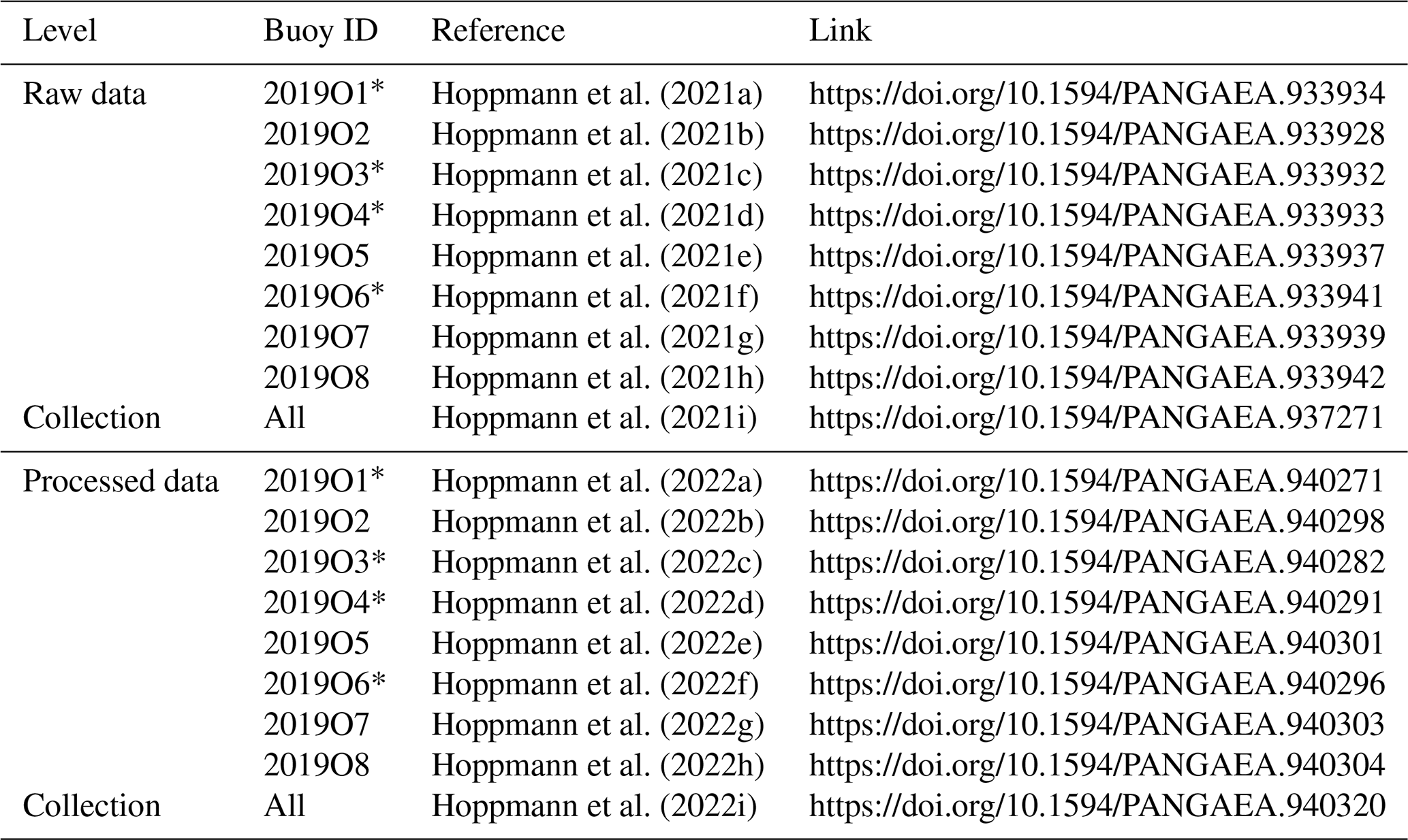
* The asterisk indicates datasets that include data from recovered SBE37 CTDs along with the transmitted buoy data.
4.2 Drift trajectories
The drift trajectories of all eight buoys are shown in Fig. 3. Their journey alongside the Central Observatory, from the deployment area north of the Laptev Sea through the Transpolar Drift until their recovery in Fram Strait, took about 10 months. The buoys traveled over the Gakkel Ridge from the Amundsen Basin to the Nansen Basin in March/April 2020. The drift accelerated strongly from June onwards upon reaching the Yermak Plateau. While a detailed discussion of the drift pattern is beyond the scope of this paper, it should be noted that the relative positions of the buoys within the array did not change much before finally entering the Fram Strait area (Fig. 3).
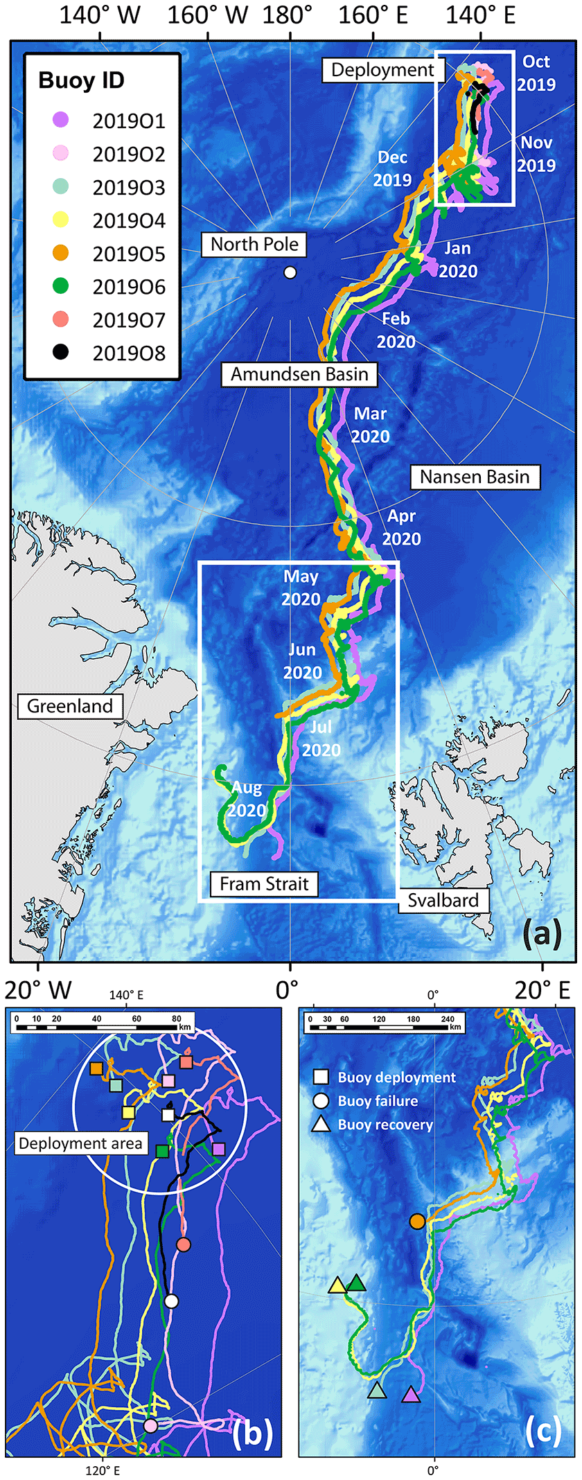
Figure 3Maps of buoy drift trajectories through the Arctic Transpolar Drift between October 2019 and August 2020. (a) Overview map. (b) Initial setup north of the Laptev Sea and the first weeks of the drift. (c) The last weeks of the drift in Fram Strait. Squares indicate deployment locations, and circles indicate locations of failure or recovery. Bathymetric data were obtained from the International Bathymetric Chart of the Arctic Ocean (IBCAO) project (Jakobsson et al., 2020). Coastline data are taken from Wessel and Smith (1996).
4.3 Oceanographic data
In the following, we take a closer look at each of the processed datasets shown as time series plots in Figs. 4 and 5. The corresponding T−S diagrams are provided as a supplement in the Appendix (Fig. A1). As stated earlier, we refer to a specific instrument time series by the buoy name with the nominal instrument depth. For simplicity, we use the buoy name and instrument references as a synonym for the time series itself.

Figure 4Time series of main variables recorded by buoys for which internal CTD data are available. (a) 2019O1, (b) 2019O3, (c) 2019O4, and (d) 2019O6. Each of the subplots in panels (a) to (d) show seawater temperature (ITS-90), seawater practical salinity (PSS-78), instrument depth, buoy drift speed (gray), and surface temperature (blue indicates submerged in seawater, and red indicates not submerged). For the oceanographic variables, we only show “1 – good” and “2 – modified” values.
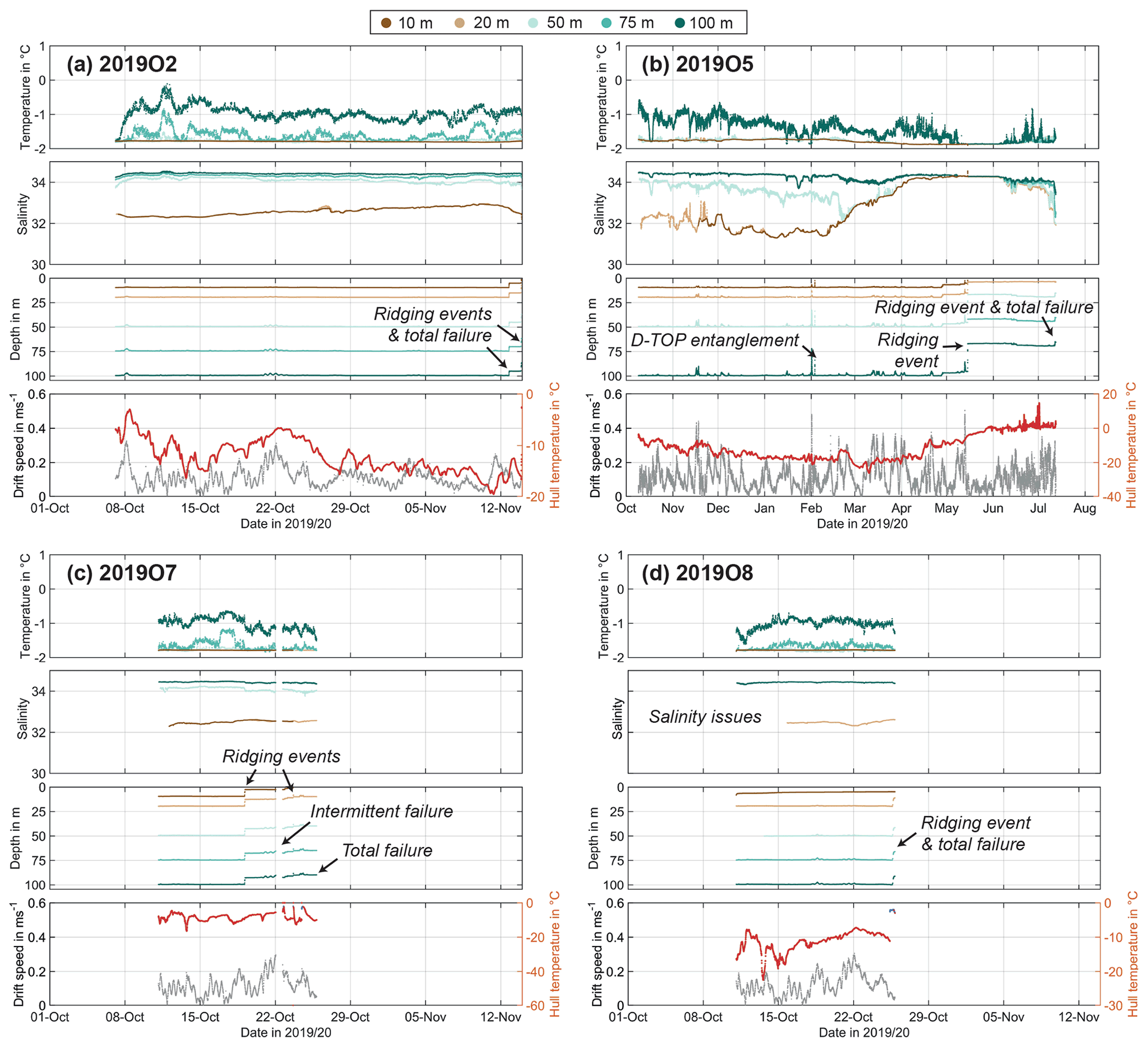
Figure 5Time series of main variables recorded by buoys for which internal CTD data are not available. (a) 2019O2, (b) 2019O5, (c) 2019O7, and (d) 2019O8. Each of the subplots in panels (a) to (d) show seawater temperature (ITS-90), seawater practical salinity (PSS-78), instrument depth, buoy drift speed (gray), and surface temperature (blue indicates submerged in seawater, and red indicates not submerged). For the oceanographic variables, we only show “1 – good” and “2 – modified” values.
Buoy 2019O1 (Fig. 4a) was generally performing well, except for some problems at the beginning of its life cycle. 2019O1-10m and 2019O1-20m show a suspiciously low salinity for the first few days after deployment, before adjusting to consistent levels. 2019O1-75m and 2019O1-100m had the same issue at the very beginning (lasting only a few hours), while it took 2019O1-50m a full 2.5 weeks before plausible salinity data were collected. We assume that these instruments were affected by ice formation in the conductivity cells, which is a known issue when instruments are submerged while still being much colder than the seawater. We acknowledge, however, that it is quite unusual that it takes an instrument such a long time to recover, even when installed in seawater at freezing point. An alternative explanation is that bubbles were trapped in the conductivity cell that were eventually able to escape the cell. This is also a known issue, especially with shallow deployments. After this initial adjustment period, 2019O1 continued to collect reasonable data throughout its operational time. The unit was recovered on 5 August 2020.
Buoy 2019O2 (Fig. 5a) started fine before all instruments were suddenly lifted by 5 m over 1 h during an event on 12 November 2019. They remained in place for 1 d before they were lifted again by 8 m in a similar event. The buoy was lost immediately afterward on 13 November 2019.
Buoy 2019O3 (Fig. 4b) was fine initially, but 2019O3-50m stopped working after several hours following the deployment and never resumed any data transmission. The other four instruments were performing well throughout their operational time. During an event on 17 February 2020, all remaining CTDs were substantially lifted although there was no particularly strong drift at that time. 2019O3-10m and 2019O3-20m were even lifted to depths as shallow as the ice base, which is unusual. The only explanation is that the buoy tether became entangled with the co-deployed DTOP free floating profiler, which possibly moved closer to the SIT as a result of converging pack ice conditions. The sensors returned to their original depths after ∼ 30 min and continued to measure correctly until the buoy was recovered on 3 August 2020.
Buoy 2019O4 (Fig. 4c) was fine from the start. Due to an unintentionally high measurement interval of 30 s, 2019O4-75m ran out of power on 20 April 2020 after a period of intermittent failures starting on 11 January 2020. The buoy and all other CTDs continued to work well until recovery on 14 August 2020.
Buoy 2019O5 (Fig. 5b) showed some moderate problems. 2019O5-75m stopped communicating upon deployment. 2019O5-10m started to exhibit inductive modem communication issues at the end of October 2019. This began with sporadic missing measurements in the buoy's transmission afterward, which subsequently became more frequent throughout November when roughly half of the measurements were blanks. In the second half of November, the issue gradually disappeared, with transmissions returning to normal on 27 November. From late December 2019 onwards, 2019O5-20m and 2019O5-50m started to exhibit similar issues, again first sporadic and then almost continuously (roughly half of the measurements affected). Interestingly, this problem never affected both sensors at the same time, and the missing transmissions were always alternating and sometimes more or less periodic. From mid-January onwards, 2019O5-50m recovered from this problem, and transmissions were completely normal from the end of January 2020 onwards. However, the issue with 2019O5-20m persisted until mid-February 2020, with failures still being somewhat periodic at times, when the blanks slowly started to decrease. In late February, the problem with 2019O5-20m was also gone, when 2019O5-100m started to exhibit blanks, with the same pattern. It was first sporadic, then much more frequently. In late April, they became only sporadic again, with a very small fraction of blanks during the remaining buoy lifetime. The reason for this behavior remains unclear. On 14/15 May 2020, a drastic event took place. 2019O5-50m and 2019O5-100m showed a sudden 30 m pressure decrease on that day, suggesting that the entire buoy was lifted by that amount, presumably in a substantial ridging event. Communication to 2019O5-10m was lost in the process, as it was probably torn off the tether. At the same time, however, 2019O5-75m started to transmit data again, at a current depth of ∼ 45 m (as expected as the event lifted the instrument from a nominal depth of 75 m). 2019O5-20m was only lifted by 16 m, to a depth of 4 m, suggesting that it was pushed down along the tether by the resistance of the ice bottom. Surprisingly, the sensor survived this incident. The buoy kept collecting reasonable data via the four remaining CTDs (2019O5-20m presumably directly from the ice base), and, interestingly, without any further inductive modem issues. There were two more events, on 13 and 16 June 2020, during which three of the four instruments suddenly moved down 1 m each, except for 2019O5-20m, which was then at 3.8 m and presumably stuck in the ice. Another event during which the buoy was lifted by 4 m occurred on 12 July 2020, shortly before the buoy stopped transmitting any more data.
Buoy 2019O6 (Fig. 4d) was generally performing well but suffered from an issue with the inductive modem link as well. 2019O6-10m had some minor conductivity cell issues in the first few days after deployment. Inductive modem issues with all instruments on the tether became worse from November 2019 onwards but significantly improved again from 13 April 2020 for unknown reasons. These issues resulted in erroneous values being recorded by the buoy (in contrast to the problems with 2019O5, where measurements were just blank), leading to a large number of outliers in the raw dataset. On 3 August 2020, all CTDs exhibited a sudden increase in pressure of 0.5 dbar, probably related to a draining melt pond (although the submergence sensor was never triggered) or a similar effect that caused the surface buoy to slightly drop. The unit was recovered on 13 August 2020.
Similar to 2019O2, buoys 2019O7 and 2019O8 (Fig. 5c, d) were also fairly short-lived. 2019O7-75m suffered from conductivity cell issues upon deployment and did not recover. All instruments were lifted by 7 m during an event on 19 October 2019. The instruments were at stable depths for a few days before they were lifted again over a few days between 22 and 24 October. 2019O7-10m was lost eventually, and the buoy stopped transmitting entirely on 26 October 2019. There were three instruments on 2019O8 that had issues with the conductivity cell upon deployment, which lasted until the end of its (short) operational time. On 25 October 2019, all instruments were lifted by 10 m over a few hours, with 2019O8-10m being stuck at the ice bottom and pushed down the tether. A few hours after that, the buoy stopped transmitting.
In this section, we assess the quality of the oceanographic data and discuss the general instrument performance. We showcase the strength of the deployment concept and potential of the dataset as a whole and discuss the wider role of the data and, in particular, the potential within the framework of MOSAiC.
5.1 Data quality and validation
In addition to a general data plausibility and consistency check among individual (independent) CTDs installed on the same tether as performed during the data processing, there are a few other methods to assess the general data reliability and quality. These will be elaborated on in this section.
5.1.1 Post-deployment calibration
The CTDs were manufactured and laboratory-calibrated by Sea-Bird only 2 months before deployment. Post-deployment calibration was performed at Sea-Bird for three sets of CTDs (2019O3, 2019O4, and 2019O6; 15 in total) in July 2021. 2019O1 was redeployed during the final MOSAiC leg a few weeks later as 2020O10 (not shown here), so the five corresponding CTDs were not available for post-deployment calibration. We decided to not apply any correction to the temperature and salinity data based on this calibration information (see below). Furthermore, the schedule of our logistics operations and tasks on board did not allow us to conduct in situ calibration for each CTD using the higher-accuracy ship-based Sea-Bird SBE 911plus system. However, there was the possibility of cross-validation to concurrent observations taken nearby during visits to the sites (see Sect. 5.1.2).
Table 4Temperature offset and conductivity drift from post-deployment calibration. Pressure (not shown) did not drift at all. This information is provided here for reference. Corrections have not been applied to the data (see text). Note: SN is the serial number, Pre-cal is the pre-calibration date, and Post-cal is the post-calibration date.
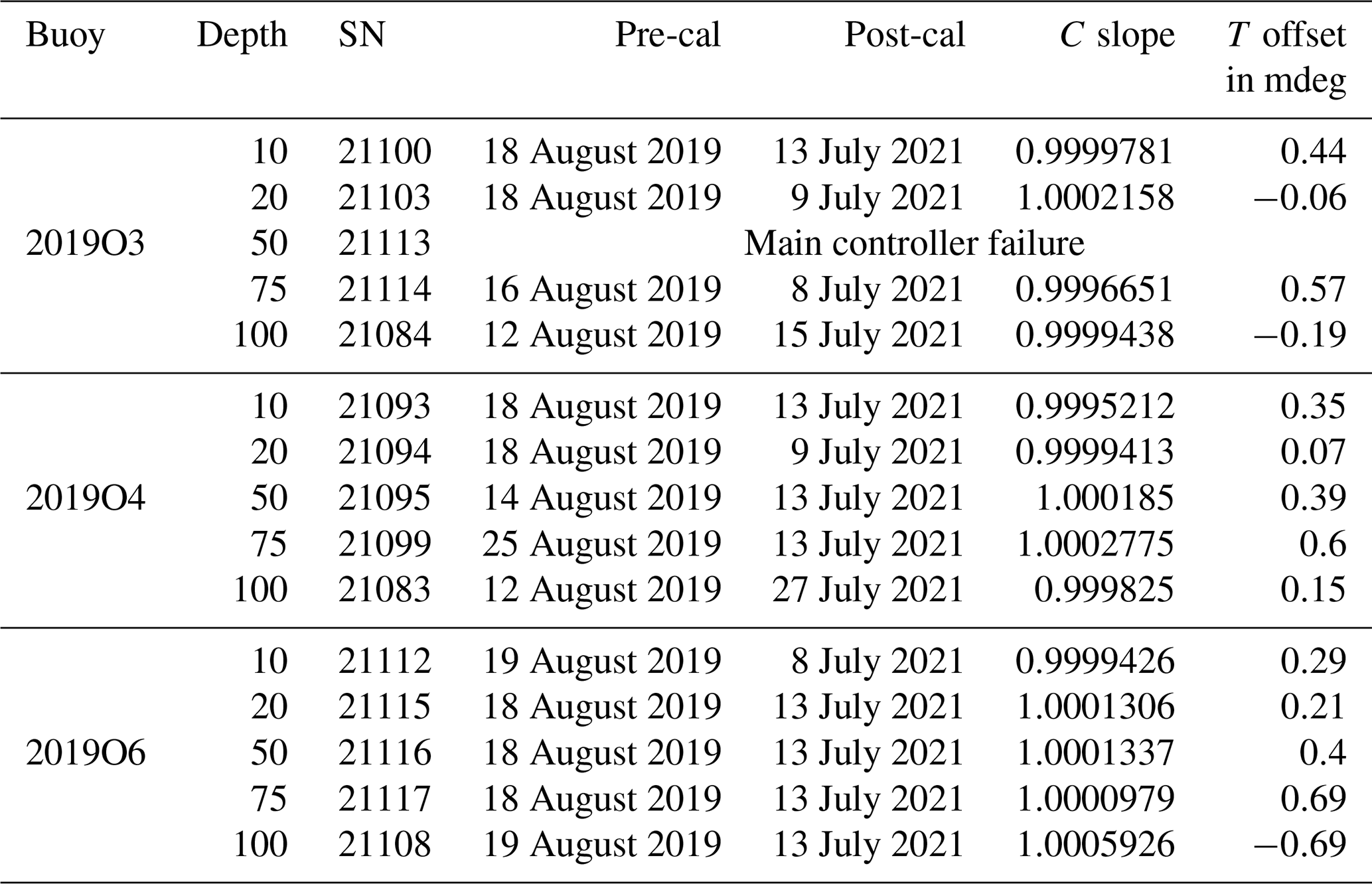
The results of the post-deployment calibration were within normal limits for this instrument type (Table 4). While a temperature offset and conductivity drift correction of the data according to Sea-Bird's Application Note 31 was considered, we decided not to apply this procedure to the present dataset for the following reasons: the offset in temperature (usually by electronic drift) was generally of the order of ±0.0005 ∘C, which is within the noise level of the instruments. In addition, the calibration sheets show that the main contribution to the calculated offset stemmed from bath temperatures >5 ∘C, which is much higher than ambient temperatures for the upper 100 m of the water column. The conductivity drift, which is usually a result of fouling processes within the conductivity cell, was also generally low. The problem with fouling is that the usual assumption of a linear change is not necessarily true. Such a change can also occur suddenly, and the calibration does not account for the timing. Assuming the fouling would lead to a linear drift of the cell, the instrument is treated in various ways and exposed to different environmental conditions between the recovery and the actual calibration. It is usually cleaned, packed, transported, and stored, so the calibration results are not necessarily reflecting the conditions under which the instrument took the measurements. Finally, an open question is whether to perform the linear correction between the calibration dates (as recommended by Sea-Bird) or between deployment and recovery, where fouling can occur. Due to these issues, we decided to not correct the values measured by each sensor and, instead, validate the measurements to estimate how reliable they are. The results from our procedure suggest that all instruments in Table 4 can be considered reliable. As a final note, 2019O3-50m was diagnosed with a main controller failure and was replaced on warranty.
5.1.2 Validation using independent measurements
A wealth of hydrographic data were collected during MOSAiC at different times and places as part of the physical oceanography program. Specifically intended to validate the buoy data in situ, several deployment sites were revisited during April and May 2020. Several water column profiles were obtained using two handheld unpumped, self-recording CTDs (SST 48M, Sea & Sun Technology GmbH, Germany; hereafter referred to as SST-CTD). The instrument was mounted on the line of a fishing rod with a battery-powered winch to measure profiles of temperature, salinity, and pressure in the upper water column. A total of five SST-CTD profiles were taken at different deployment sites (see Table A1).
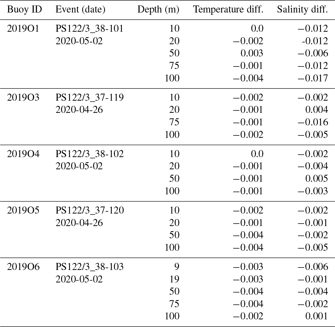
In addition to the manufacturer's calibration, the two SST-CTDs were mounted on a standard ship-based high-accuracy CTD rosette system for in situ calibration (Sea-Bird SBE 911plus, hereafter referred to as ship CTD for simplicity) to validate the sensors themselves. These intercalibration exercises were carried out in February and July 2020, close in time to the validation casts at the buoy sites, to minimize the potential influence of unaccounted sensor drift. The results of these calibration casts showed a deviation of pressure in both SST-CTDs from the ship CTD of approximately 1 m at 100 m depth. This has been taken into account for the comparison to the buoy data by smoothing the profile. SST-CTD salinity and temperature deviations were largest within the halocline and upper permanent pycnocline (e.g., Polyakov et al., 2013), as can be expected for this kind of intercalibration procedure. The average salinity and temperature offsets were 0.008 and 0.006 ∘C, respectively, and have been corrected. For comparison with the buoy data, the SST-CTD validation profiles have been smoothed using a Savitzky–Golay filter (window size of 31, corresponding to about 3.5 m). An example of the comparison is shown in Fig. 6. The average deviation values between SST-CTD and the buoy temperature and salinity are ∘C and , respectively, which is within the stated accuracy of the SST-CTD sensors (given by the manufacturer as 0.002 ∘C for T and 0.002 ms cm−1 for C). In conclusion, the CTDs on the buoys show very good agreement with the intercalibrated SST-CTDs after a measurement period of 6 months.

Figure 6Comparison between SST-CTD and 2019O3 data on 26 April 2020. Red and blue lines represent salinity and temperature recorded by the SST-CTD, respectively. Circles represent buoy data closest in time to the SST-CTD cast. The colored dots show the values of the corresponding buoy CTD within 30 min before and after the SST-CTD cast. Buoy data at 10 and 20 m are hidden below the circles.
5.1.3 Data transfer issues
An additional source of error that is not necessarily obvious is introduced by quirks in the inductive modem communication between the instruments and the surface package of the buoy. The reliability of the oceanographic data polled from the individual CTDs by the surface electronics via the inductive modem link can be assessed by comparing the buoy dataset to the data collected internally by the 20 individual CTDs that were recovered in August 2020. This comparison confirmed that the buoys generally operated as intended. However, in the case of 2019O6, this comparison helped us to identify and remove a large number of outliers that seemingly resulted from an (unknown) issue in the inductive modem communication.
The transmission of data via iridium (in this case the short-burst data protocol) may sometimes be unstable due to a variety of reasons, but this usually only leads to the unit not being able to transfer a data package in the first place or, more rarely, to the loss of individual data packages. This technique generally does not introduce errors in the recorded data itself, as far as we are aware.
5.2 Properties of an observed eddy
Here we present a prominent example of the type of features observable with the present instrumentation and overall approach – a mesoscale eddy that passed through the buoy array in February 2020. During that time, the MOSAiC observatory drifted towards the northwest at an average velocity of about 0.13 m s−1. The number of loops was considerably less than during the previous November and December (Fig. 7a). The buoys drifted along a pronounced surface salinity gradient from less saline water in the southeast to more saline in the northwest (Fig. 7). The lateral gradients of salinity and temperature are evident from both the time series along each buoy track and in the observations between different buoys.

Figure 7Preliminary observations of an eddy passing through the DN in February 2020. (a) Trajectories and observed salinity at 10 m depth of five buoys (colored) along with trajectory of R/V Polarstern (black) between 2 and 20 February 2020. Triangles indicate the buoy positions on 2 February. The black horizontal lines with numbered bars indicate the start and end positions of the times in panels (c) and (d), where changing water properties were observed by the corresponding buoy. (b) T−S diagram of buoy data at 20 and 100 m depth during 1 to 20 February 2020 (red) and 20 February to 1 March 2020 (blue). (c, d) Temperature and salinity recorded at four different depths by buoys 2019O1, 2019O4, and 2019O6. The line colors correspond to the triangle colors in panel (a).
Although our measurements are confined to discrete depths, the CTD records at 20 and 50 m can still indicate the minimum mixed-layer depth if they show equal temperature and salinity. Thereby, we infer from the records of 2019O4 and 2019O6 that the depth of the upper ocean mixed layer (ML) increased to >50 m from about mid-February onwards. This is in agreement with less frequent observations by an ocean profiler (Rabe et al., 2022).
Changes in water properties with time at 20 and 100 m depths are shown in the temperature–salinity diagram in Fig. 7b. The mixed-layer salinity increased with a corresponding decrease in temperature along the freezing line during February. At the same time, salinity and temperature at 100 m decreased. An increase in mixed-layer salinity could be partly explained by a combination of the upward mixing of deep salty water from below and salt rejection during ice formation from above, both forced by two February storms with wind speeds up to 16 m s−1 and surface air temperatures of around −15 ∘C. However, close-by, near-daily measurements of the vertical mixing properties with a dedicated microstructure probe at the central observatory did not show significant mixing underneath the halocline (Schulz et al., 2022). Further mixed-layer deepening occurred into early April (Fig. 4) when the ML depth reached 100 m. Between February and April, the drift path of the buoys was about 340 km, equivalent to a 270 km straight line distance. They drifted across the front associated with the transition from the Transpolar Drift to the warm and salty inflow of water of Atlantic origin through Fram Strait. These types of upper-ocean salinity gradients generally provide a high potential to form eddies.
During 7–10 February, rapid changes in the water properties were registered by 2019O4, 2019O6, and, to a lesser extent, 2019O1. 2019O6 (blue triangle and lines in Fig. 7) and 2019O4 (red triangle and lines in Fig. 7) registered these changes 4 and 1 d in advance of R/V Polarstern reaching the same location, respectively. The evolution of the observed salinity values shows a tendency for saltier waters appearing at depths shallower than ∼ 50 m and fresher waters deeper than 70 m. For example, the salinity decreased by 0.22 and 0.17 at 100 and 75 m, respectively, and increased by 0.5 at 50 m depth for buoy 2019O6. Temperature evolution is less conclusive since most measurements were within the range of the cold halocline layer. This feature indicates the presence of an eddy with the approximate geographical locations registered by the buoys as shown by two short lines (beginning and end) on the buoy tracks (Fig. 7a) and colored shaded areas in Fig. 7c and d, with buoy temperatures and salinities at four depths of 20, 50, 75, and 100 m. The CTDs at 10 m depth show mostly the same water properties as those at 20 m. Line colors correspond to the triangle colors of the buoys in Fig. 7a. This event was also observed by the current measurements obtained by the shipboard acoustic Doppler current profiler (ADCP). It shows the presence of the eddy between 11 and 13 February (Sandra Tippenhauer, personal communication, 2021), and the location is denoted in Fig. 7a (black dots on the dashed line). Most likely, the ship drifted close to the center of the eddy. It exhibited a rather symmetric current structure, with the minimum speed in the center and currents on the sides in opposite directions with speeds up to 20 m s−1. The estimated diameter of the eddy based on the buoy drift was about 30 km. A detailed description of the eddy properties is beyond the scope of this paper and is the subject of ongoing work.
It is important to note that the drift speed increased from 0.04 to 0.2 m s−1 between 7 and 14 February. Thereby, the time interval during which the eddy was observed by different buoys decreased, while the drifting distance (or eddy diameter) remained similar. At the same time, 2019O3 and 2019O5 do not show significant changes at a depth of 100 m. Both buoys were located to the northeast of the ship. Likely, they were too far away from the core of the eddy to register a measurable signal.
All three buoys that registered the eddy encountered similar anomalies in temperature and salinity. The salinity decreased by 0.22 and 0.17 at 100 and 75 m, respectively, and increased by 0.5 at 50 m depth, with a corresponding temperature decrease of 0.3, 0.12, and 0.05 ∘C for buoy 2019O6. We also calculated the bulk buoyancy frequency, , using measurements between 50 and 100 m. The result shows that N decreased during the passing of the eddy from ∼ 8 to 5.7 cph for 2019O6, from ∼ 7.2 to 5.1 cph for 201904, and from ∼ 6 to 4 cph for 2019O1. If we use the simplest way to calculate the first-mode baroclinic Rossby radius, using with a constant N=5 cph and H=4500 m, then LR is around 14 km (corresponding to a diameter of 28 km) and close to the estimated diameter of the eddy. The distributed nature of the buoys allows a fully synoptic assessment at different points across the array, which could not have been achieved by just one buoy.
5.3 Wider scope of the dataset
The example in Sect. 5.2 shows how our data can be used to study mesoscale features in the upper Arctic Ocean. The wider scope of science questions that could be studied with the data is broad – the seasonality could be explored further, as could the variability along the pathways of the Arctic Transpolar Drift (e.g., Stedmon et al., 2021). In particular, the buoy data fill the winter gap common to manual in situ observations that are often carried out during seasonally limited ship surveys. The high temporal resolution allows for studying passing transient and submesoscale phenomena, as the buoys acted as a quasi-stationary platform, depending on drift speed. On the other hand, during times of faster drift, the systems measured the upper ocean quasi-synoptically over submesoscales.
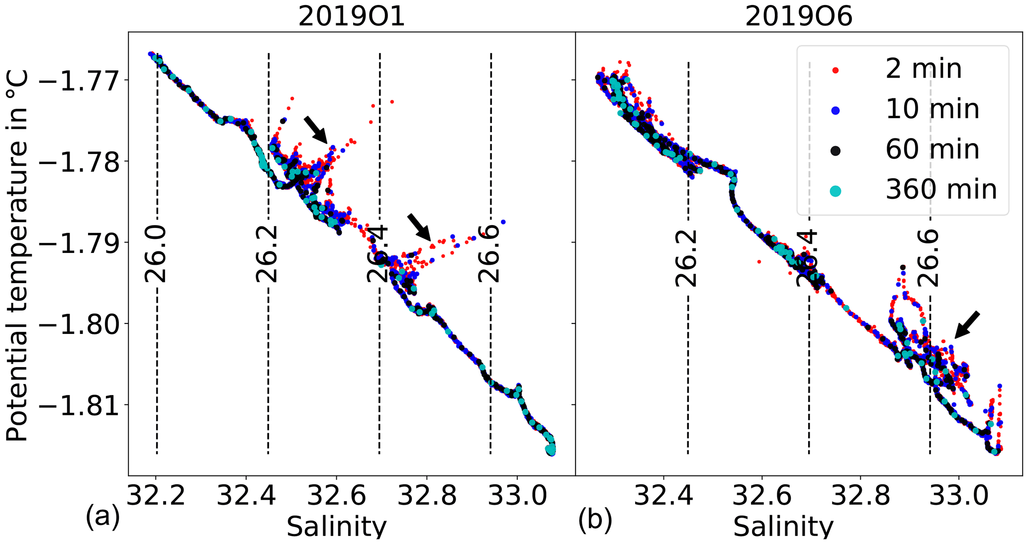
Figure 8T−S diagram of observations during 12 February–1 March 2020, at 20 m from (a) 2019O1 and (b) 2019O6. Dots with different colors denote different temporal resolutions. Black arrows highlight features that can be only resolved with high-resolution data.
This allows us to observe small-scale spatiotemporal variability in temperature and salinity that may be overlooked by traditional platforms. Measurements along a fixed isobath on a scale of hours correspond to a spatial resolution of ∼ 10 km (e.g., like those collected from ships or ITPs) and normally resolve mesoscale features. This may be illustrated by subsampling our buoy data at an interval of 60 and 360 min (Fig. 8), revealing a near-surface frontal structure in the T−S diagram with warmer (colder) and fresher (saltier) water at either side of the front. Note that the nominal capacity of our buoys allows <10 min ( km) resolution data; thus, the buoys further capture phenomena hidden in this frontal structure. For example, there appears to be a density compensation process with warmer, saline waters compensating those with lower temperature and salinity (see black arrows in Fig. 8a). Another nearby buoy sees the same large-scale front but may additionally observe a local thermohaline intrusion within the front (see black arrow in Fig. 8b).
The significance of submesoscale circulation has been shown in numerous studies, highlighting the associated strong vertical velocity (Biddle and Swart, 2020; Mahadevan et al., 2010), restratification processes (Timmermans et al., 2012; du Plessis et al., 2019), conversion of potential to eddy kinetic energy (Zhang et al., 2019), and feedback between ice and ocean currents around filaments in the MIZ (von Appen et al., 2018). These physical processes can significantly influence biogeochemical conditions and the ecosystem (Fadeev et al., 2021; Kaiser et al., 2021). Yet, the submesoscale is largely limited to regional models or idealized process simulations (e.g., Manucharyan and Timmermans, 2013; Manucharyan and Thompson, 2017) and largely out of reach for state-of-the-art numerical ocean general circulation models, thus necessitating appropriate parameterizations (e.g., Lévy et al., 2012).
Analyzing our dataset further could make use of horizontal wavenumber spectra that can give insights into the length scales of variability induced by submesoscale restratification and internal waves (Marcinko et al., 2015; Timmermans et al., 2012). Furthermore, submesoscale eddies and filaments between mesoscale features can be studied with this piecewise quasi-synoptic dataset.
The scientific results of these potential studies, and the data, could serve to validate numerical models of the ice–ocean system and the fully coupled Earth system. The observations can also serve as input to numerical models, either to initialize or force a simulation or to provide input for assimilation. Finally, the GPS data recorded by our buoys were also used to create the official drift trajectories for several of the main sites of the DN (Nicolaus et al., 2021b).
Collections of the presented raw and processed datasets are available under https://doi.org/10.1594/PANGAEA.937271 (Hoppmann et al., 2021i) and https://doi.org/10.1594/PANGAEA.940320 (Hoppmann et al., 2022i). An overview of all individual raw datasets (including unprocessed buoy and CTD data) and all fully processed and quality-controlled individual datasets is given in Table 3. The MATLAB code used to create the processed datasets is available on request.
We have shown results from a unique deployment of several ice-tethered buoy systems measuring temperature and salinity in the upper 100 m of the central Arctic Ocean. These systems were part of the MOSAiC expedition, a year-long drift of the German icebreaker R/V Polarstern in 2019/2020. The deployment concept was specifically designed to observe mesoscale and, to a lesser degree, submesoscale variability, including internal waves, in the ocean mixed layer and upper halocline throughout different seasons and across the Eurasian Basin. Additionally, the buoys provided valuable oceanographic data as a complement to various other co-located multidisciplinary ice-tethered buoy systems and the overall MOSAiC work program. The buoy systems generally performed well, with a few expected failures due to ice deformation, particularly as the sea ice environment was even more dynamic than anticipated. An added value was obtained by recovering four of the eight buoys, yielding data at an even higher temporal resolution. We have shown through a validation approach that the temperature and salinity measurements by our buoy systems are accurate and capable of showing details of an upper ocean eddy during the Arctic winter. Additionally, post-deployment calibration only showed minor sensor drift. The dataset is expected to be of significant value, for example, for future process studies, even beyond MOSAiC, and for the validation of numerical models aiming to better understand the role of the crucially important though barely studied Arctic Ocean in the Earth's climate system.
On a final note, buoy 2019O1 was redeployed in the new ice camp of MOSAiC-Leg5 close to the North Pole in August 2020 as 2020O10. As of August 2022, this buoy has reached Iceland, although the CTDs ran out of power a few months earlier. Since this deployment was not part of the array, we decided to not include it in this paper. However, we will apply a similar processing to this dataset, for consistency, and to future deployments of similar buoys that are already planned for 2022, 2023, and 2024.
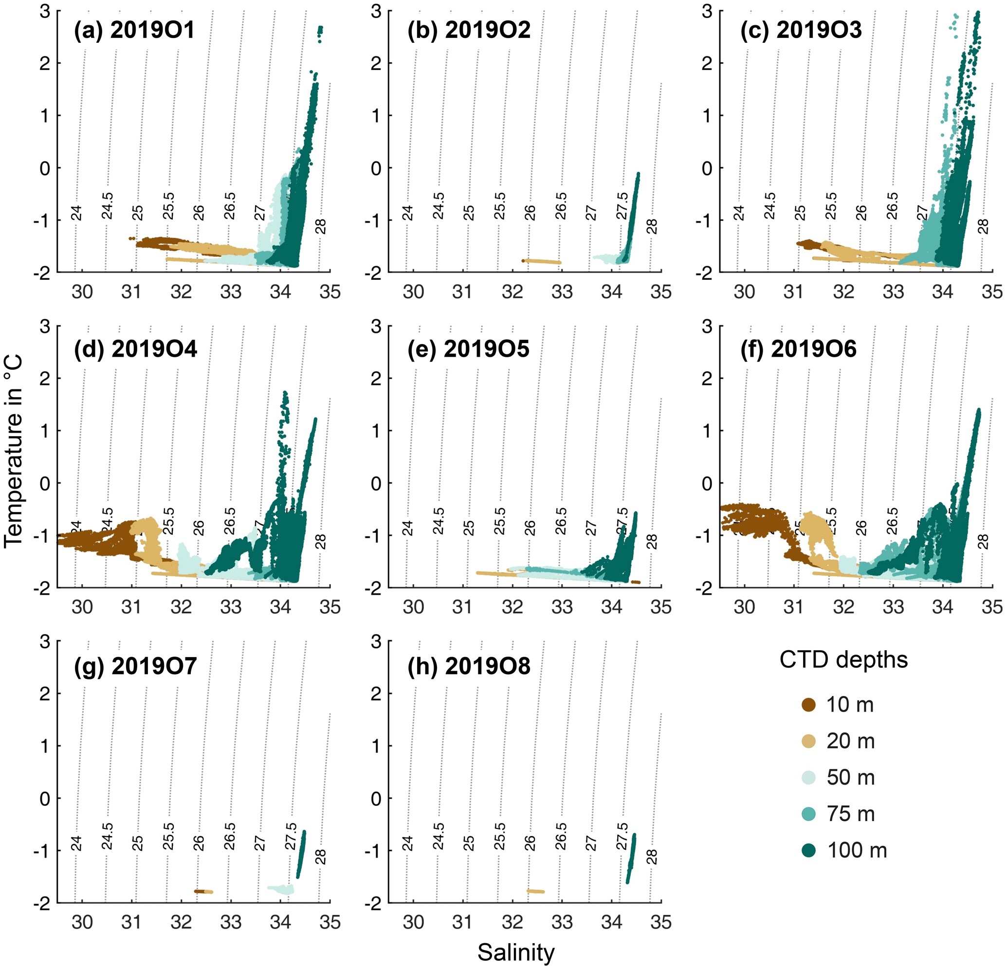
Figure A1T−S diagrams based on the processed datasets collected by all eight buoys during their drift through the central Arctic as part of the MOSAiC DN. Note that these diagrams strongly depend on the operation lifetime of the corresponding buoy.
Table A1Comparison of SST-CTD profiles with buoy measurements for validation.
BR was responsible for the initial conceptualization of the study. The methodology was proposed by BR and further enhanced by MH, YCF, and IK. BR and MH were responsible for the project administration. MH and YCF deployed the instruments in the field. MH was responsible for the data curation, prepared the original draft, and visualized the data. IK conducted the data validation and eddy studies. All authors contributed to the review and editing of the paper.
The contact author has declared that none of the authors has any competing interests.
Publisher’s note: Copernicus Publications remains neutral with regard to jurisdictional claims in published maps and institutional affiliations.
We thank Andy Sybrandy and Pacific Gyre, for building the buoys, Kathrin Riemann-Campe and Marcel Nicolaus, for their help with the intermediate data provision via https://www.meereisportal.de/ (last access: 29 September 2022), and Wilken-Jon von Appen, for his input to the introduction. We thank the crews of the research vessels Akademik Fedorov, Akademik Tryoshnikov, and R/V Polarstern, as well as the helicopter company Naryan-Marski, for their great logistical support that made this study possible. We extend our gratitude to all participants of these expeditions, particularly to the MOSAiC School, for their field assistance during the setup phase, to Janin Schaffer and the Leg3 team, for their effort to collect the validation data, and to Matthew Shupe, Julia Regnery, Kirstin Schulz and the Leg4 team, for the recovery of the instruments. Full acknowledgements are available in Nixdorf et al. (2021). Finally, we thank the three anonymous reviewers and the editor, Giuseppe M. R. Manzella, for their valuable comments which significantly improved the quality of this paper.
Data presented in this paper were produced as part of the international Multidisciplinary drifting Observatory for the Study of the Arctic Climate (MOSAiC) with the tag MOSAiC20192020 (grant nos. AWI_PS122_00 and AF-MOSAiC-1_00). The study was partly funded through the PACES II (Polar regions And Coasts in the changing Earth System) program and the FRAM (FRontiers in Arctic marine Monitoring) strategic investment by the Helmholtz Association. The instruments were funded by the Alfred-Wegener-Institut as part of the MIDO (Multidisciplinary Ice-based Distributed Observatory) infrastructure program. The study contributes to the Changing Arctic Ocean (CAO) program, jointly funded by the UKRI Natural Environment Research Council (NERC) and the German Federal Ministry for Education and Research (BMBF), as part of the project Advective Pathways of nutrients and key Ecological substances in the ARctic (APEAR; grant nos. NE/R012865/1, NE/R012865/2, and 03V01461). This research further contributes to the project EPICA in the scope of the theme MARE:N – Polarforschung/MOSAiC funded by the BMBF (grant no. 03F0889A) and the European Commission for EU H2020 (project Arctic PASSION; grant no. 101003472).
This paper was edited by Giuseppe M. R. Manzella and reviewed by three anonymous referees.
Athanase, M., Sennéchael, N., Garric, G., Koenig, Z., Boles, E., and Provost, C.: New Hydrographic Measurements of the Upper Arctic Western Eurasian Basin in 2017 Reveal Fresher Mixed Layer and Shallower Warm Layer Than 2005–2012 Climatology, J. Geophys. Res.-Oceans, 124, 1091–1114, https://doi.org/10.1029/2018JC014701, 2019. a
Beszczynska-Möller, A., Fahrbach, E., Schauer, U., and Hansen, E.: Variability in Atlantic water temperature and transport at the entrance to the Arctic Ocean, 1997–2010, ICES J. Mar. Sci., 69, 852–863, https://doi.org/10.1093/icesjms/fss056, 2012. a
Biddle, L. C. and Swart, S.: The Observed Seasonal Cycle of Submesoscale Processes in the Antarctic Marginal Ice Zone, J. Geophys. Res.-Oceans, 125, e2019JC015587, https://doi.org/10.1029/2019JC015587, 2020. a
Bretherton, F. P., Davis, R. E., and Fandry, C. B.: A technique for objective analysis and design of oceanographic experiments applied to MODE-73, Deep Sea Research and Oceanographic Abstracts, 23, 559–582, https://doi.org/10.1016/0011-7471(76)90001-2, 1976. a
Capet, X., McWilliams, J. C., Molemaker, M. J., and Shchepetkin, A. F.: Mesoscale to submesoscale transition in the California Current system. Part I: Flow structure, eddy flux, and observational tests, J. Phys. Oceanogr., 38, 29–43, https://doi.org/10.1175/2007JPO3671.1, 2008. a
Chelton, D. B., DeSzoeke, R. A., Schlax, M. G., El Naggar, K., and Siwertz, N.: Geographical Variability of the First Baroclinic Rossby Radius of Deformation, J. Phys. Oceanogr., 28, 433–460, https://doi.org/10.1175/1520-0485(1998)028<0433:GVOTFB>2.0.CO;2, 1998. a
D'Asaro, E., Lee, C., Rainville, L., Harcourt, R., and Thomas, L.: Enhanced Turbulence and Energy Dissipation at Ocean Fronts, Science, 332, 318–322, https://doi.org/10.1126/science.1201515, 2011. a
D'Asaro, E. A.: Observations of small eddies in the Beaufort Sea, J. Geophys. Res.-Oceans, 93, 6669–6684, https://doi.org/10.1029/JC093iC06p06669, 1988. a
du Plessis, M., Swart, S., Ansorge, I. J., Mahadevan, A., and Thompson, A. F.: Southern Ocean Seasonal Restratification Delayed by Submesoscale Wind–Front Interactions, J. Phys. Oceanogr., 49, 1035–1053, https://doi.org/10.1175/JPO-D-18-0136.1, 2019. a
Fadeev, E., Wietz, M., von Appen, W.-J., Iversen, M. H., Nöthig, E.-M., Engel, A., Grosse, J., Graeve, M., and Boetius, A.: Submesoscale physicochemical dynamics directly shape bacterioplankton community structure in space and time, Limnol. Oceanogr., 66, 2901–2913, https://doi.org/10.1002/lno.11799, 2021. a
Ferrari, R. and Wunsch, C.: Ocean Circulation Kinetic Energy: Reservoirs, Sources, and Sinks, Annu. Rev. Fluid Mech., 41, 253–282, https://doi.org/10.1146/annurev.fluid.40.111406.102139, 2008. a
Gallaher, S. G., Stanton, T. P., Shaw, W. J., Cole, S. T., Toole, J. M., Wilkinson, J. P., Maksym, T., and Hwang, B.: Evolution of a Canada Basin ice-ocean boundary layer and mixed layer across a developing thermodynamically forced marginal ice zone, J. Geophys. Res.-Oceans, 121, 6223–6250, https://doi.org/10.1002/2016JC011778, 2016. a
Gaube, P., Chelton, D. B., Samelson, R. M., Schlax, M. G., and O'Neill, L. W.: Satellite observations of mesoscale eddy-induced Ekman pumping, J. Phys. Oceanogr., 45, 104–132, https://doi.org/10.1175/JPO-D-14-0032.1, 2015. a
Gill, A., Green, J., and Simmons, A.: Energy partition in the large-scale ocean circulation and the production of mid-ocean eddies, Deep Sea Research and Oceanographic Abstracts, 21, 509–528, https://doi.org/10.1016/0011-7471(74)90010-2, 1974. a
Gommenginger, C., Chapron, B., Hogg, A., Buckingham, C., Fox-Kemper, B., Eriksson, L., Soulat, F., Ubelmann, C., Ocampo-Torres, F., Nardelli, B. B., Griffin, D., Lopez-Dekker, P., Knudsen, P., Andersen, O., Stenseng, L., Stapleton, N., Perrie, W., Violante-Carvalho, N., Schulz-Stellenfleth, J., Woolf, D., Isern-Fontanet, J., Ardhuin, F., Klein, P., Mouche, A., Pascual, A., Capet, X., Hauser, D., Stoffelen, A., Morrow, R., Aouf, L., Breivik, O., Fu, L.-L., Johannessen, J. A., Aksenov, Y., Bricheno, L., Hirschi, J., Martin, A. C. H., Martin, A. P., Nurser, G., Polton, J., Wolf, J., Johnsen, H., Soloviev, A., Jacobs, G. A., Collard, F., Groom, S., Kudryavtsev, V., Wilkin, J., Navarro, V., Babanin, A., Martin, M., Siddorn, J., Saulter, A., Rippeth, T., Emery, B., Maximenko, N., Romeiser, R., Graber, H., Azcarate, A. A., Hughes, C. W., Vandemark, D., Silva, J. d., Leeuwen, P. J. V., Naveira-Garabato, A., Gemmrich, J., Mahadevan, A., Marquez, J., Munro, Y., Doody, S., and Burbidge, G.: SEASTAR: A Mission to Study Ocean Submesoscale Dynamics and Small-Scale Atmosphere-Ocean Processes in Coastal, Shelf and Polar Seas, Frontiers in Marine Science, 6, 457, https://doi.org/10.3389/fmars.2019.00457, 2019. a
Hatakeyama, K., Hosono, M., Shimada, K., Kikuchi, T., and Nishino, S.: JAMSTEC Compact Arctic Drifter (J-CAD): A new Generation drifting buoy to observe the Arctic Ocean, Journal of the Japan Society for Marine Surveys and Technology, 13, 1_55–1_68, https://ui.adsabs.harvard.edu/abs/2012JJSMS..13.1.55H (last access: 29 September 2022), 2012. a
Hewitt, C. D., Golding, N., Zhang, P., Dunbar, T., Bett, P. E., Camp, J., Mitchell, T. D., and Pope, E.: The Process and Benefits of Developing Prototype Climate Services – Examples in China, Journal of Meteorological Research, 34, 893–903, https://doi.org/10.1007/s13351-020-0042-6, 2020. a
Hill, V. J., Light, B., Steele, M., and Zimmerman, R. C.: Light Availability and Phytoplankton Growth Beneath Arctic Sea Ice: Integrating Observations and Modeling, J. Geophys. Res.-Oceans, 123, 3651–3667, https://doi.org/10.1029/2017JC013617, 2018. a
Hoppmann, M., Kuznetsov, I., Fang, Y.-C., and Rabe, B.: Raw seawater temperature, conductivity and salinity obtained at different depths by CTD buoy 2019O1 as part of the MOSAiC Distributed Network, PANGAEA [data set], https://doi.org/10.1594/PANGAEA.933934, 2021a. a
Hoppmann, M., Kuznetsov, I., Fang, Y.-C., and Rabe, B.: Raw seawater temperature, conductivity and salinity obtained at different depths by CTD buoy 2019O2 as part of the MOSAiC Distributed Network, PANGAEA [data set], https://doi.org/10.1594/PANGAEA.933928, 2021b. a
Hoppmann, M., Kuznetsov, I., Fang, Y.-C., and Rabe, B.: Raw seawater temperature, conductivity and salinity obtained at different depths by CTD buoy 2019O3 as part of the MOSAiC Distributed Network, PANGAEA [data set], https://doi.org/10.1594/PANGAEA.933932, 2021c. a
Hoppmann, M., Kuznetsov, I., Fang, Y.-C., and Rabe, B.: Raw seawater temperature, conductivity and salinity obtained at different depths by CTD buoy 2019O4 as part of the MOSAiC Distributed Network, PANGAEA [data set], https://doi.org/10.1594/PANGAEA.933933, 2021d. a
Hoppmann, M., Kuznetsov, I., Fang, Y.-C., and Rabe, B.: Raw seawater temperature, conductivity and salinity obtained at different depths by CTD buoy 2019O5 as part of the MOSAiC Distributed Network, PANGAEA [data set], https://doi.org/10.1594/PANGAEA.933937, 2021e. a
Hoppmann, M., Kuznetsov, I., Fang, Y.-C., and Rabe, B.: Raw seawater temperature, conductivity and salinity obtained at different depths by CTD buoy 2019O6 as part of the MOSAiC Distributed Network, PANGAEA [data set], https://doi.org/10.1594/PANGAEA.933941, 2021f. a
Hoppmann, M., Kuznetsov, I., Fang, Y.-C., and Rabe, B.: Raw seawater temperature, conductivity and salinity obtained at different depths by CTD buoy 2019O7 as part of the MOSAiC Distributed Network, PANGAEA [data set], https://doi.org/10.1594/PANGAEA.933939, 2021g. a
Hoppmann, M., Kuznetsov, I., Fang, Y.-C., and Rabe, B.: Raw seawater temperature, conductivity and salinity obtained at different depths by CTD buoy 2019O8 as part of the MOSAiC Distributed Network, PANGAEA [data set], https://doi.org/10.1594/PANGAEA.933942, 2021h. a
Hoppmann, M., Kuznetsov, I., Fang, Y.-C., and Rabe, B.: Raw seawater temperature, conductivity and salinity obtained with CTD buoys as part of the MOSAiC Distributed Network, PANGAEA [data set], https://doi.org/10.1594/PANGAEA.937271, 2021i. a, b, c
Hoppmann, M., Kuznetsov, I., Fang, Y.-C., and Rabe, B.: Processed seawater temperature, conductivity and salinity obtained at different depths by CTD buoy 2019O1 as part of the MOSAiC Distributed Network, PANGAEA [data set], https://doi.org/10.1594/PANGAEA.940271, 2022a. a
Hoppmann, M., Kuznetsov, I., Fang, Y.-C., and Rabe, B.: Processed seawater temperature, conductivity and salinity obtained at different depths by CTD buoy 2019O2 as part of the MOSAiC Distributed Network, PANGAEA [data set], https://doi.org/10.1594/PANGAEA.940298, 2022b. a
Hoppmann, M., Kuznetsov, I., Fang, Y.-C., and Rabe, B.: Processed seawater temperature, conductivity and salinity obtained at different depths by CTD buoy 2019O3 as part of the MOSAiC Distributed Network, PANGAEA [data set], https://doi.org/10.1594/PANGAEA.940282, 2022c. a
Hoppmann, M., Kuznetsov, I., Fang, Y.-C., and Rabe, B.: Processed seawater temperature, conductivity and salinity obtained at different depths by CTD buoy 2019O4 as part of the MOSAiC Distributed Network, PANGAEA [data set], https://doi.org/10.1594/PANGAEA.940291, 2022d. a
Hoppmann, M., Kuznetsov, I., Fang, Y.-C., and Rabe, B.: Processed seawater temperature, conductivity and salinity obtained at different depths by CTD buoy 2019O5 as part of the MOSAiC Distributed Network, PANGAEA [data set], https://doi.org/10.1594/PANGAEA.940301, 2022e. a
Hoppmann, M., Kuznetsov, I., Fang, Y.-C., and Rabe, B.: Processed seawater temperature, conductivity and salinity obtained at different depths by CTD buoy 2019O6 as part of the MOSAiC Distributed Network, PANGAEA [data set], https://doi.org/10.1594/PANGAEA.940296, 2022f. a
Hoppmann, M., Kuznetsov, I., Fang, Y.-C., and Rabe, B.: Processed seawater temperature, conductivity and salinity obtained at different depths by CTD buoy 2019O7 as part of the MOSAiC Distributed Network, PANGAEA [data set], https://doi.org/10.1594/PANGAEA.940303, 2022g. a
Hoppmann, M., Kuznetsov, I., Fang, Y.-C., and Rabe, B.: Processed seawater temperature, conductivity and salinity obtained at different depths by CTD buoy 2019O8 as part of the MOSAiC Distributed Network, PANGAEA [data set], https://doi.org/10.1594/PANGAEA.940304, 2022h. a
Hoppmann, M., Kuznetsov, I., Fang, Y.-C., and Rabe, B.: Processed data of CTD buoys 2019O1 to 2019O8 as part of the MOSAiC Distributed Network, PANGAEA [data set], https://doi.org/10.1594/PANGAEA.940320, 2022i. a, b, c
Huang, X., Wang, Z., Zhang, Z., Yang, Y., Zhou, C., Yang, Q., Zhao, W., and Tian, J.: Role of Mesoscale Eddies in Modulating the Semidiurnal Internal Tide: Observation Results in the Northern South China Sea, J. Phys. Oceanogr., 48, 1749–1770, https://doi.org/10.1175/JPO-D-17-0209.1, 2018. a
Ilicak, M., Drange, H., Wang, Q., Gerdes, R., Aksenov, Y., Bailey, D., Bentsen, M., Biastoch, A., Bozec, A., Boening, C., Cassou, C., Chassignet, E., Coward, A. C., Curry, B., Danabasoglu, G., Danilov, S., Fernandez, E., Fogli, P. G., Fujii, Y., Griffies, S. M., Iovino, D., Jahn, A., Jung, T., Large, W. G., Lee, C., Lique, C., Lu, J., Masina, S., Nurser, A. J. G., Roth, C., Salas y Melia, D., Samuels, B. L., Spence, P., Tsujino, H., Valcke, S., Voldoire, A., Wang, X., and Yeager, S. G.: An assessment of the Arctic Ocean in a suite of interannual CORE-II simulations. Part III: Hydrography and fluxes, Ocean Model., 100, 141–161, https://doi.org/10.1016/j.ocemod.2016.02.004, 2016. a
Jackson, K., Wilkinson, J., Maksym, T., Beckers, J., Haas, C., Meldrum, D., and Mackenzie, D.: A Novel and Low Cost Sea Ice Mass Balance Buoy, J. Atmos. Ocean. Tech., 30, 2676–2688, https://doi.org/10.1175/jtech-d-13-00058.1, 2013. a
Jakobsson, M., Mayer, L. A., Bringensparr, C., Castro, C. F., Mohammad, R., Johnson, P., Ketter, T., Accettella, D., Amblas, D., An, L., Arndt, J. E., Canals, M., Casamor, J. L., Chauché, N., Coakley, B., Danielson, S., Demarte, M., Dickson, M.-L., Dorschel, B., Dowdeswell, J. A., Dreutter, S., Fremand, A. C., Gallant, D., Hall, J. K., Hehemann, L., Hodnesdal, H., Hong, J., Ivaldi, R., Kane, E., Klaucke, I., Krawczyk, D. W., Kristoffersen, Y., Kuipers, B. R., Millan, R., Masetti, G., Morlighem, M., Noormets, R., Prescott, M. M., Rebesco, M., Rignot, E., Semiletov, I., Tate, A. J., Travaglini, P., Velicogna, I., Weatherall, P., Weinrebe, W., Willis, J. K., Wood, M., Zarayskaya, Y., Zhang, T., Zimmermann, M., and Zinglersen, K. B.: The International Bathymetric Chart of the Arctic Ocean Version 4.0, Scientific Data, 7, 176, https://doi.org/10.1038/s41597-020-0520-9, 2020. a
Jochum, M. and Murtugudde, R. (Eds.): Physical Oceanography: Developments Since 1950, 1st Edn., Springer-Verlag New York, https://doi.org/10.1007/0-387-33152-2, 2006. a
Kaiser, P., Hagen, W., von Appen, W.-J., Niehoff, B., Hildebrandt, N., and Auel, H.: Effects of a submesoscale oceanographic filament on zooplankton dynamics in the Arctic marginal ice zone, Frontiers in Marine Research, 8, 625395, https://doi.org/10.3389/fmars.2021.625395, 2021. a
Kikuchi, T., Inoue, J., and Langevin, D.: Argo-type profiling float observations under the Arctic multiyear ice, Deep-Sea Res. I, 54, 1675–1686, https://doi.org/10.1016/j.dsr.2007.05.011, 2007. a
Koenig, Z., Provost, C., Villacieros-Robineau, N., Sennechael, N., and Meyer, A.: Winter ocean-ice interactions under thin sea ice observed by IAOOS platforms during N-ICE2015: Salty surface mixed layer and active basal melt, J. Geophys. Res.-Oceans, 121, 7898–7916, https://doi.org/10.1002/2016JC012195, 2016. a
Krumpen, T., Birrien, F., Kauker, F., Rackow, T., von Albedyll, L., Angelopoulos, M., Belter, H. J., Bessonov, V., Damm, E., Dethloff, K., Haapala, J., Haas, C., Harris, C., Hendricks, S., Hoelemann, J., Hoppmann, M., Kaleschke, L., Karcher, M., Kolabutin, N., Lei, R., Lenz, J., Morgenstern, A., Nicolaus, M., Nixdorf, U., Petrovsky, T., Rabe, B., Rabenstein, L., Rex, M., Ricker, R., Rohde, J., Shimanchuk, E., Singha, S., Smolyanitsky, V., Sokolov, V., Stanton, T., Timofeeva, A., Tsamados, M., and Watkins, D.: The MOSAiC ice floe: sediment-laden survivor from the Siberian shelf, The Cryosphere, 14, 2173–2187, https://doi.org/10.5194/tc-14-2173-2020, 2020. a
Lee, C. M., Thomson, J., Team, M. I. Z., and Team, A. S. S.: An Autonomous Approach to Observing the Seasonal Ice Zone in the Western Arctic, Oceanography, 30, 56–68, https://doi.org/10.5670/oceanog.2017.222, 2017. a
Lévy, M., Iovino, D., Resplandy, L., Klein, P., Madec, G., Tréguier, A.-M., Masson, S., and Takahashi, K.: Large-scale impacts of submesoscale dynamics on phytoplankton: Local and remote effects, Ocean Model., 43-44, 77–93, https://doi.org/10.1016/j.ocemod.2011.12.003, 2012. a
Lévy, M., Franks, P., and Smith, K. S.: The role of submesoscale currents in structuring marine ecosystems, Nat. Commun., 9, 4758, https://doi.org/10.1038/s41467-018-07059-3, 2018. a
Mahadevan, A.: The Impact of Submesoscale Physics on Primary Productivity of Plankton, Annu. Rev. Mar. Sci., 8, 161–184, https://doi.org/10.1146/annurev-marine-010814-015912, 2016. a
Mahadevan, A., Tandon, A., and Ferrari, R.: Rapid changes in mixed layer stratification driven by submesoscale instabilities and winds, J. Geophys. Res.-Oceans, 115, C03017, https://doi.org/10.1029/2008JC005203, 2010. a, b
Manley, T. O. and Hunkins, K.: Mesoscale eddies of the Arctic Ocean, J. Geophys. Res.-Oceans, 90, 4911–4930, https://doi.org/10.1029/JC090iC03p04911, 1985. a
Manucharyan, G. E. and Thompson, A. F.: Submesoscale Sea Ice-Ocean Interactions in Marginal Ice Zones, J. Geophys. Res.-Oceans, 122, 9455–9475, https://doi.org/10.1002/2017JC012895, 2017. a
Manucharyan, G. E. and Timmermans, M.-L.: Generation and Separation of Mesoscale Eddies from Surface Ocean Fronts, J. Phys. Oceanogr., 43, 2545–2562, https://doi.org/10.1175/JPO-D-13-094.1, 2013. a
Marcinko, C. L., Martin, A. P., and Allen, J. T.: Characterizing horizontal variability and energy spectra in the Arctic Ocean halocline, J. Geophys. Res.-Oceans, 120, 436–450, https://doi.org/10.1002/2014JC010381, 2015. a
McDougall, T. J. and Barker, P. M.: Getting started with TEOS-10 and the Gibbs Seawater (GSW) Oceanographic Toolbox, 28 pp., SCOR/IAPSO WG127, ISBN 978-0-646-55621-5, 2011. a, b
McGillicuddy, D. J.: Mechanisms of Physical-Biological-Biogeochemical Interaction at the Oceanic Mesoscale, Annu. Rev. Mar. Sci., 8, 125–159, https://doi.org/10.1146/annurev-marine-010814-015606, 2016. a
McWilliams, J. C.: Maps from the Mid-Ocean Dynamics Experiment: Part I. Geostrophic Streamfunction, J. Phys. Oceanogr., 6, 810–827, https://doi.org/10.1175/1520-0485(1976)006<0810:MFTMOD>2.0.CO;2, 1976. a
McWilliams, J. C.: Submesoscale currents in the ocean, P. R. Soc. A, 472, 20160117, https://doi.org/10.1098/rspa.2016.0117, 2016. a
Nicolaus, M., Hoppmann, M., Arndt, S., Hendricks, S., Katlein, C., Nicolaus, A., Rossmann, L., Schiller, M., and Schwegmann, S.: Snow Depth and Air Temperature Seasonality on Sea Ice Derived From Snow Buoy Measurements, Frontiers in Marine Science, 8, 655446, https://doi.org/10.3389/fmars.2021.655446, 2021a. a
Nicolaus, M., Riemann-Campe, K., Hutchings, J. K., Granskog, M. A., Krishfield, R. A., Lei, R., Li, T., Hoppmann, M., and Rabe, B.: Drift trajectories of the main sites of the Distributed Network of MOSAiC 2019/2020, PANGAEA [data set], https://doi.org/10.1594/PANGAEA.937204, 2021b. a
Nicolaus, M., Perovich, D. K., Spreen, G., Granskog, M. A., von Albedyll, L., Angelopoulos, M., Anhaus, P., Arndt, S., Belter, H. J., Bessonov, V., Birnbaum, G., Brauchle, J., Calmer, R., Cardellach, E., Cheng, B., Clemens-Sewall, D., Dadic, R., Damm, E., de Boer, G., Demir, O., Dethloff, K., Divine, D. V., Fong, A. A., Fons, S., Frey, M. M., Fuchs, N., Gabarró, C., Gerland, S., Goessling, H. F., Gradinger, R., Haapala, J., Haas, C., Hamilton, J., Hannula, H.-R., Hendricks, S., Herber, A., Heuzé, C., Hoppmann, M., Høyland, K. V., Huntemann, M., Hutchings, J. K., Hwang, B., Itkin, P., Jacobi, H.-W., Jaggi, M., Jutila, A., Kaleschke, L., Katlein, C., Kolabutin, N., Krampe, D., Kristensen, S. S., Krumpen, T., Kurtz, N., Lampert, A., Lange, B. A., Lei, R., Light, B., Linhardt, F., Liston, G. E., Loose, B., Macfarlane, A. R., Mahmud, M., Matero, I. O., Maus, S., Morgenstern, A., Naderpour, R., Nandan, V., Niubom, A., Oggier, M., Oppelt, N., Pätzold, F., Perron, C., Petrovsky, T., Pirazzini, R., Polashenski, C., Rabe, B., Raphael, I. A., Regnery, J., Rex, M., Ricker, R., Riemann-Campe, K., Rinke, A., Rohde, J., Salganik, E., Scharien, R. K., Schiller, M., Schneebeli, M., Semmling, M., Shimanchuk, E., Shupe, M. D., Smith, M. M., Smolyanitsky, V., Sokolov, V., Stanton, T., Stroeve, J., Thielke, L., Timofeeva, A., Tonboe, R. T., Tavri, A., Tsamados, M., et al.: Overview of the MOSAiC expedition: Snow and sea ice, Elementa: Science of the Anthropocene, 10, 000046, https://doi.org/10.1525/elementa.2021.000046, 2022. a
Nixdorf, U., Dethloff, K., Rex, M., Shupe, M., Sommerfeld, A., Perovich, D. K., Nicolaus, M., Heuzé, C., Rabe, B., Loose, B., Damm, E., Gradinger, R., Fong, A., Maslowski, W., Rinke, A., Kwok, R., Spreen, G., Wendisch, M., Herber, A., Hirsekorn, M., Mohaupt, V., Frickenhaus, S., Immerz, A., Weiss-Tuider, K., König, B., Mengedoht, D., Regnery, J., Gerchow, P., Ransby, D., Krumpen, T., Morgenstern, A., Haas, C., Kanzow, T., Rack, F. R., Saitzev, V., Sokolov, V., Makarov, A., Schwarze, S., Wunderlich, T., Wurr, K., and Boetius, A.: MOSAiC Extended Acknowledgement, Zenodo, https://doi.org/10.5281/zenodo.5541624, 2021. a
Nurser, A. J. G. and Bacon, S.: The Rossby radius in the Arctic Ocean, Ocean Sci., 10, 967–975, https://doi.org/10.5194/os-10-967-2014, 2014. a, b
Ocean University of China: The Drift-Towing Ocean Profiler, http://coas.ouc.edu.cn/pogoc/2021/0713/c9714a342585/page.htm (last access: 29 September 2022), 2021. a
Polyakov, I. V., Pnyushkov, A. V., Rember, R., Padman, L., Carmack, E. C., and Jackson, J. M.: Winter Convection Transports Atlantic Water Heat to the Surface Layer in the Eastern Arctic Ocean, J. Phys. Oceanogr., 43, 2142–2155, https://doi.org/10.1175/JPO-D-12-0169.1, 2013. a
Porter, M., Henley, S. F., Orkney, A., Bouman, H. A., Hwang, B., Dumont, E., Venables, E. J., and Cottier, F.: A Polar Surface Eddy Obscured by Thermal Stratification, Geophys. Res. Lett., 47, e2019GL086281, https://doi.org/10.1029/2019GL086281, 2020. a
Rabe, B., Heuzé, C., Regnery, J., Aksenov, Y., Allerholt, J., Athanase, M., Bai, Y., Basque, C., Bauch, D., Baumann, T. M., Chen, D., Cole, S. T., Craw, L., Davies, A., Damm, E., Dethloff, K., Divine, D. V., Doglioni, F., Ebert, F., Fang, Y.-C., Fer, I., Fong, A. A., Gradinger, R., Granskog, M. A., Graupner, R., Haas, C., He, H., He, Y., Hoppmann, M., Janout, M., Kadko, D., Kanzow, T., Karam, S., Kawaguchi, Y., Koenig, Z., Kong, B., Krishfield, R. A., Krumpen, T., Kuhlmey, D., Kuznetsov, I., Lan, M., Laukert, G., Lei, R., Li, T., Torres-Valdés, S., Lin, L., Lin, L., Liu, H., Liu, N., Loose, B., Ma, X., McKay, R., Mallet, M., Mallett, R. D. C., Maslowski, W., Mertens, C., Mohrholz, V., Muilwijk, M., Nicolaus, M., O’Brien, J. K., Perovich, D., Ren, J., Rex, M., Ribeiro, N., Rinke, A., Schaffer, J., Schuffenhauer, I., Schulz, K., Shupe, M. D., Shaw, W., Sokolov, V., Sommerfeld, A., Spreen, G., Stanton, T., Stephens, M., Su, J., Sukhikh, N., Sundfjord, A., Thomisch, K., Tippenhauer, S., Toole, J. M., Vredenborg, M., Walter, M., Wang, H., Wang, L., Wang, Y., Wendisch, M., Zhao, J., Zhou, M., and Zhu, J.: Overview of the MOSAiC expedition: Physical oceanography, Elementa: Science of the Anthropocene, 10, 00062, https://doi.org/10.1525/elementa.2021.00062, 2022. a, b, c
Schulz, K., Mohrholz, V., Fer, I., Janout, M., Hoppmann, M., Schaffer, J., and Koenig, Z.: A full year of turbulence measurements from a drift campaign in the Arctic Ocean 2019–2020, Sci. Data, 9, 472, https://doi.org/10.1038/s41597-022-01574-1, 2022. a
Shupe, M. D., Rex, M., Blomquist, B., Persson, P. O. G., Schmale, J., Uttal, T., Althausen, D., Angot, H., Archer, S., Bariteau, L., Beck, I., Bilberry, J., Bucci, S., Buck, C., Boyer, M., Brasseur, Z., Brooks, I. M., Calmer, R., Cassano, J., Castro, V., Chu, D., Costa, D., Cox, C. J., Creamean, J., Crewell, S., Dahlke, S., Damm, E., de Boer, G., Deckelmann, H., Dethloff, K., Dütsch, M., Ebell, K., Ehrlich, A., Ellis, J., Engelmann, R., Fong, A. A., Frey, M. M., Gallagher, M. R., Ganzeveld, L., Gradinger, R., Graeser, J., Greenamyer, V., Griesche, H., Griffiths, S., Hamilton, J., Heinemann, G., Helmig, D., Herber, A., Heuzé, C., Hofer, J., Houchens, T., Howard, D., Inoue, J., Jacobi, H.-W., Jaiser, R., Jokinen, T., Jourdan, O., Jozef, G., King, W., Kirchgaessner, A., Klingebiel, M., Krassovski, M., Krumpen, T., Lampert, A., Landing, W., Laurila, T., Lawrence, D., Lonardi, M., Loose, B., Lüpkes, C., Maahn, M., Macke, A., Maslowski, W., Marsay, C., Maturilli, M., Mech, M., Morris, S., Moser, M., Nicolaus, M., Ortega, P., Osborn, J., Pätzold, F., Perovich, D. K., Petäjä, T., Pilz, C., Pirazzini, R., Posman, K., Powers, H., Pratt, K. A., Preußer, A., Quéléver, L., Radenz, M., Rabe, B., Rinke, A., Sachs, T., Schulz, A., Siebert, H., Silva, T., Solomon, A., Sommerfeld, A., et al.: Overview of the MOSAiC expedition – Atmosphere, Elementa: Science of the Anthropocene, 10, 00060, https://doi.org/10.1525/elementa.2021.00060, 2022. a
Smith, K. S.: The geography of linear baroclinic instability in Earth's oceans, J. Mar. Res., 65, 655–683, https://doi.org/10.1357/002224007783649484, 2007. a, b
Stedmon, C. A., Amon, R. M. W., Bauch, D., Bracher, A., Gonçalves-Araujo, R., Hoppmann, M., Krishfield, R., Laney, S., Rabe, B., Reader, H., and Granskog, M. A.: Insights into Water Mass Circulation and Origins in the Central Arctic Ocean from in-situ Dissolved Organic Matter Fluorescence, J. Geophys. Res.-Oceans, 126, e2021JC017407, https://doi.org/10.1029/2021JC017407, 2021. a
Steele, M.: UpTempO buoys deployed in the Arctic Ocean in 2017, Arctic Data Center [data set], https://doi.org/10.18739/A2JS9H85P, 2017. a
Thomas, L. N.: Destruction of Potential Vorticity by Winds, J. Phys. Oceanogr., 35, 2457–2466, https://doi.org/10.1175/JPO2830.1, 2005. a
Thomas, L. N., Tandon, A., and Mahadevan, A.: Submesoscale Processes and Dynamics, in: Ocean Modeling in an Eddying Regime, Vol. 177, edited by: Hecht, M. W. and Hasumi, H., Geophysical Monograph Series, American Geophysical Union, https://doi.org/10.1029/177GM04, 2008. a, b
Timmermans, M.-L. and Marshall, J.: Understanding Arctic Ocean Circulation: A Review of Ocean Dynamics in a Changing Climate, J. Geophys. Res.-Oceans, 125, e2018JC014378, https://doi.org/10.1029/2018JC014378, 2020. a
Timmermans, M.-L., Cole, S., and Toole, J.: Horizontal Density Structure and Restratification of the Arctic Ocean Surface Layer, J. Phys. Oceanogr., 42, 659–668, https://doi.org/10.1175/JPO-D-11-0125.1, 2012. a, b
Toole, J., Krishfield, R., Proshutinsky, A., Ashjian, C., Doherty, K., Frye, D., Hammar, T., Kemp, J., Peters, D., Timmermans, M.-L., von der Heydt, K., Packard, G., and Shanahan, T.: Ice-tethered profilers sample the upper Arctic Ocean, Eos, Transactions American Geophysical Union, 87, 434–438, https://doi.org/10.1029/2006EO410003, 2006. a, b, c
UNESCO-IOC: Ocean Data Standards Volume 3. Recommendation for a Quality Flag Scheme for the Exchange of Oceanographic and Marine Meteorological Data, https://doi.org/10.25607/OBP-6, 2013. a, b
von Appen, W. J., Wekerle, C., Hehemann, L., Schourup-Kristensen, V., Konrad, C., and Iversen, M. H.: Observations of a Submesoscale Cyclonic Filament in the Marginal Ice Zone, Geophys. Res. Lett., 45, 6141–6149, https://doi.org/10.1029/2018GL077897, 2018. a
von Appen, W.-J., Baumann, T., Janout, M., Koldunov, N., Lenn, Y.-D., Pickart, R., Scott, R., and Wang, Q.: Eddies and the Distribution of Eddy Kinetic Energy in the Arctic Ocean, Oceanography, 35, https://doi.org/10.5670/oceanog.2022.122, 2022. a
Wang, Q., Koldunov, N. V., Danilov, S., Sidorenko, D., Wekerle, C., Scholz, P., Bashmachnikov, I. L., and Jung, T.: Eddy Kinetic Energy in the Arctic Ocean From a Global Simulation With a 1-km Arctic, Geophys. Res. Lett., 47, e2020GL088550, https://doi.org/10.1029/2020GL088550, 2020. a, b
Wessel, P. and Smith, W. H. F.: A global, self-consistent, hierarchical, high-resolution shoreline database, J. Geophys. Res.-Sol. Ea., 101, 8741–8743, https://doi.org/10.1029/96JB00104, 1996. a
Zhang, X., Dai, H., Zhao, J., and Yin, H.: Generation mechanism of an observed submesoscale eddy in the Chukchi Sea, Deep-Sea Res. Pt. I, 148, 80–87, https://doi.org/10.1016/j.dsr.2019.04.015, 2019. a
Zhao, M., Timmermans, M.-L., Cole, S., Krishfield, R., Proshutinsky, A., and Toole, J.: Characterizing the eddy field in the Arctic Ocean halocline, J. Geophys. Res.-Oceans, 119, 8800–8817, https://doi.org/10.1002/2014JC010488, 2014. a, b, c
Zhao, M., Timmermans, M.-L., Cole, S., Krishfield, R., and Toole, J.: Evolution of the eddy field in the Arctic Ocean's Canada Basin, 2005–2015, Geophys. Res. Lett., 43, 8106–8114, https://doi.org/10.1002/2016GL069671, 2016. a, b
- Abstract
- Introduction
- Material and methods
- Data processing and quality flags
- Results
- Discussion
- Code and data availability
- Conclusions and outlook
- Appendix A: Additional figures and tables
- Author contributions
- Competing interests
- Disclaimer
- Acknowledgements
- Financial support
- Review statement
- References