the Creative Commons Attribution 4.0 License.
the Creative Commons Attribution 4.0 License.
 | 16 Sep 2022
High-resolution streamflow and weather data (2013–2019) for seven small coastal watersheds in the northeast Pacific coastal temperate rainforest, Canada
Maartje C. Korver
Emily Haughton
William C. Floyd
Ian J. W. Giesbrecht
Hydrometeorological observations of small watersheds of the northeast Pacific coastal temperate rainforest (NPCTR) of North America are important to understand land to ocean ecological connections and to provide the scientific basis for regional environmental management decisions. The Hakai Institute operates a densely networked and long-term hydrometeorological monitoring observatory that fills a spatial data gap in the remote and sparsely gauged outer coast of the NPCTR. Here we present the first 5 water years (October 2013–October 2019) of high-resolution streamflow and weather data from seven small (< 13 km2) coastal watersheds. Measuring rainfall and streamflow in remote and topographically complex rainforest environments is challenging; hence, advanced and novel automated measurement methods were used. These methods, specifically for streamflow measurement, allowed us to quantify uncertainty and identify key sources of error, which varied by gauging location. Average yearly rainfall was 3267 mm, resulting in 2317 mm of runoff and 0.1087 km3 of freshwater exports from all seven watersheds per year. However, rainfall and runoff were highly variable, depending on the location and elevation. The seven watersheds have rainfall-dominated (pluvial) streamflow regimes, streamflow responses are rapid, and most water exports are driven by high-intensity fall and winter storm events. The complete hourly and 5 min interval datasets can be accessed at https://doi.org/10.21966/J99C-9C14 (Korver et al., 2021), and accompanying watershed delineations with metrics can be found at https://doi.org/10.21966/1.15311 (Gonzalez Arriola et al., 2015).
- Article
(11321 KB) - Full-text XML
- BibTeX
- EndNote


Climate and hydrology are major drivers of the physical and ecological connections between land and sea. Understanding the timing and quantities of water, sediment, nutrient, and organic matter fluxes to the ocean can provide the scientific basis for conservation and restoration of coastal environments (Fang et al., 2018), which are vulnerable to anthropogenic pressures and a warming climate (Lotze et al., 2006; Lu et al., 2018). The outer coast of the northeast Pacific coastal temperate rainforest (NPCTR) of North America is characterized by thousands of small watersheds (Gonzalez Arriola et al., 2018) with a wet and mild maritime climate, low to moderately sloped rocky terrain, and open, low productivity forests and wetland ecosystems (Banner et al., 2005). Even though total freshwater inflows to the NPCTR coast are dominated by large drainage basins that have the majority of their area located inland (Morrison et al., 2012), small coastal watersheds are thought to play an important role in supporting productive marine food webs and abundant salmon runs (Bidlack et al., 2021). However, the current network of gauging stations in the NPCTR is especially sparse among these small watersheds, due to their remote location and access limitations (Fig. 1). Consequently, estimates of weather and streamflow from that area are generally derived from models (e.g., Moore et al., 2012; Morrison et al., 2012; Hill et al., 2009; Wang et al., 2019; PRISM Climate Group, 2021). The Kwakshua Watersheds Observatory (KWO), established in 2013, helps fill this observational data gap by providing continuous and high-resolution hydrometeorological data from seven small (< 13 km2) watersheds. The KWO also monitors aquatic biogeochemistry, microbial ecology, and nearshore oceanographic conditions (Giesbrecht et al., 2021), and to date, the observatory has supported studies showing that this area of the NPCTR is a hot spot of soil organic carbon storage (McNicol et al., 2019) and that high riverine fluxes of dissolved organic matter (Oliver et al., 2017) have a significant effect on the estuarine waters of the NPCTR (St. Pierre and Oliver et al., 2020, 2021). In the regional context, the KWO is broadly representative of a rain-dominated watershed type that spans > 16 000 km2 in the NPCTR with similar climate, topography, and streamflow regimes (Giesbrecht et al., 2022).
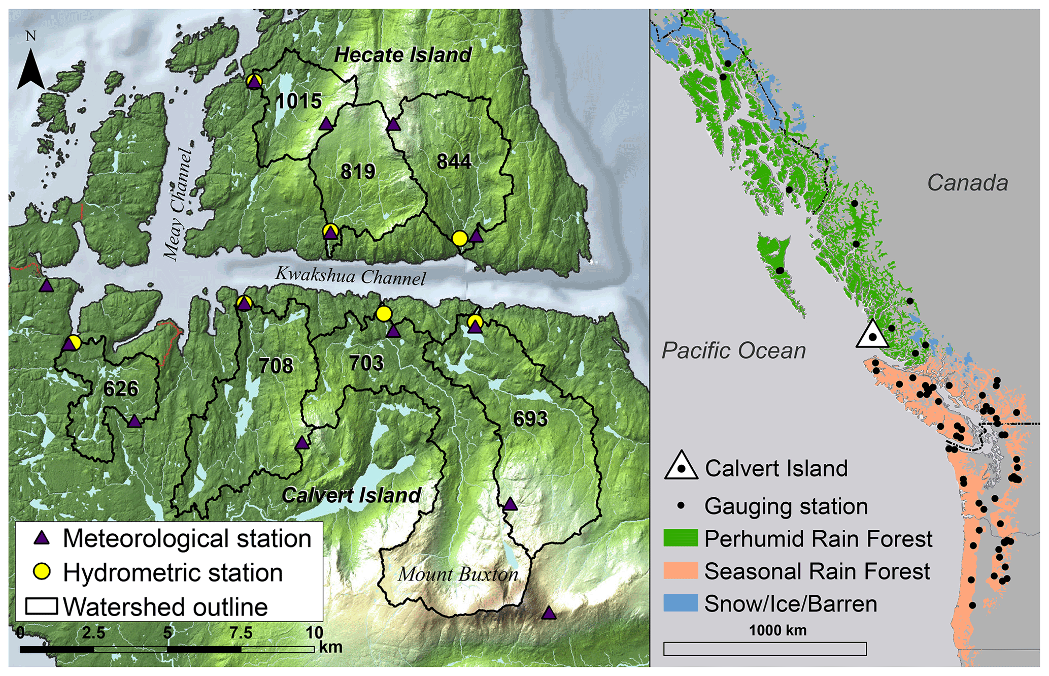
Figure 1The seven gauged watersheds at Calvert and Hecate islands on the outer coast of the northeast Pacific coastal temperate rainforest (NPCTR) of North America. Active government-operated gauging stations in small watersheds (Environment Canada stations, with a gross drainage area of < 25 km2, and United States Geological Survey (USGS) stations, with 24 h average summer flow < 1.5 m3 s−1) are shown to indicate the lack of gauging stations measuring outer coast small watersheds. The terrain relief map was created by Arriola and Holmes (2017). Regional rainforest cover is derived from the original rainforest distribution mapping of Ecotrust (1995), which reflects the rainforest subzones of Alaback (1996).
Projected changes in the NPCTR's climate – increased mean annual temperature, increased mean annual precipitation, and less precipitation as snow – are anticipated to result in a cascade of ecosystem level effects (Shanley et al., 2015; Bidlack et al., 2021) and streamflow regime changes (Déry et al., 2009). The KWO monitoring program is set up to be long term, so the hydrometeorological dataset here presented will be regularly updated to make future analyses of these anticipated system changes possible. The relatively undisturbed environment of the gauged watersheds makes the KWO particularly well suited to accommodate climate change research programs and to potentially serve within national reference hydrologic networks (Whitfield et al., 2012). In addition, the data may be useful for regional forest management decisions (e.g., Kranabetter et al., 2013; Banner et al., 2005) and engineering applications. For example, landslides triggered by heavy rain pose risks to local communities and forestry workers, but warning systems suffer from the lack of long-term quality rain gauges (Jakob et al., 2006). Landslide and flooding events are expected to increase (Sobie, 2020) as the frequency of atmospheric rivers has increased in the past few decades (Sharma and Déry, 2019) – a trend that is projected to continue (Radić et al., 2015).
This article provides a summary of streamflow and weather conditions and a characterization of catchment responses between 1 October 2013 and 30 September 2019 from the seven watersheds of the KWO. In addition, this article highlights how automation and the use of novel technologies made it possible to measure weather and streamflow in a remote environment with access limitations, complex topography, intense storms, and rapid streamflow responses, and special attention is given to the uncertainties associated with these conditions and measurement methods. It should be noted that, throughout this article, “streamflow” refers to a flow rate (m3 s−1), “discharge” describes a volume of river water (m3), and “runoff” is this volume divided by drainage area (mm). All data (continuous observations of stream discharge, rain, total precipitation, snow depth, air temperature, wind, relative humidity, and solar radiation from 7 hydrometric and 14 meteorological stations) are provided in 5 min and hourly time steps (except for snow depth data, which are exclusively provided in hourly time steps), and catchment metadata (location and catchment delineations with metrics) and calculation codes are made available (Sects. 6 and 7). High data quality is assured through systematic and thorough quality control methods.
Calvert and Hecate islands are located on the central coast of British Columbia, about 350 km northwest of Vancouver and 50 km south of Bella Bella. The islands, 325 and 46 km2, respectively, are separated by two glacially eroded sea channels, the Kwakshua and Meay channels (Fig. 1), that are connected to Fitz Hugh Sound in the east and Hakai Pass in the north. The area's relief ranges from 1012 m a.s.l. (above sea level) in the east of Calvert Island (Mount Buxton) and 495 m a.s.l. on central Hecate Island to relatively low gradient hummocky terrain in the west. The landscape is characterized by extensive wetlands, bog forests, and bog woodlands (Green, 2014; Thompson et al., 2016) on faulted and folded intrusive igneous bedrock (primarily quartz diorite; Roddick, 1996). The soils are thin (< 70 cm on average), rich in organics, and have formed in sandy colluvium and patchy morainal deposits (Oliver et al., 2017), resulting in a soil landscape with limited water storage potential. Forest stands are generally short with open canopies, and the tree composition is dominated by western redcedar, yellow cedar, shore pine, and western hemlock (Thompson et al., 2016; Hoffman et al., 2021). Understory and wetland plants include bryophytes, salal, deer fern, Sphagnum mosses, and sedges.
Calvert and Hecate islands are located within the Hakai Lúxvbálís Conservancy (protected area) and the unceded territories of the Haíłzaqv and Wuikinuxv Nations. The study watersheds have no dams or diversions, no active roads, and little evidence of historic logging, except in some shoreline areas which are now well forested. Old-growth forests are extensive, and tree ages commonly exceed 250 years (Hoffman et al., 2021). Fire is typically infrequent in the coastal temperate rainforest, yet recent work has revealed legacies of long-term cultural burning near village sites in this area (Hoffman et al., 2016). More broadly, indigenous oral history and archaeological evidence describe at least 13 000 years of human activity in the area (McLaren et al., 2015, 2018), and active stewardship is ongoing.
The KWO design captures the seven largest (3.0 to 12.8 km2) watersheds draining into Kwakshua and Meay channels, signified as 626, 708, 703, and 693 (Calvert Island) and 1015, 819, and 844 (Hecate Island). The watersheds are on average 68 % forested, 24 % non-forested but vegetated (mainly wetlands with short vegetation), 4 % non-vegetated (mainly exposed bedrock), and 4 % covered by lakes (Thompson et al., 2016; Table 1). Contrasting watershed features are summarized by the topography, the presence of lakes, and land cover. Watersheds 626, 708, and 1015 drain overall low gradient terrain, 819 and 844 reach medium elevations (465 and 495 m a.s.l.), and 693 and 703 drain Mount Buxton (1012 m a.s.l.), which is the only area experiencing permanent seasonal snow cover. Watersheds 708 and 1015 encompass a large lake (28–30 ha), located centrally and near the outlet, respectively, watershed 693 is characterized by a chain of four larger lakes (> 5 ha) near the outlet, watersheds 819 and 844 have almost no lake cover, and numerous small lakes and ponds (< 1 ha) are scattered across 626, 708, and 703. In terms of land cover, the Hecate Island watersheds are overall more forested than the watersheds on Calvert Island (more wetlands with short vegetation), 626 stands out for its relatively sparse forest cover and high amount of wetlands/unvegetated areas, and watershed 703 is largely unvegetated at high elevations (exposed bedrock; Table 1).
Table 1Main characteristics of the seven gauged watersheds.
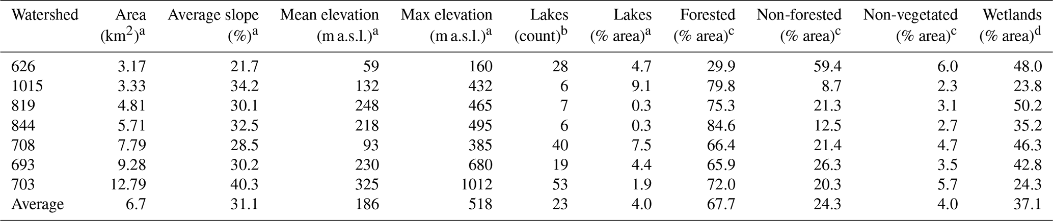
a Reproduced from Gonzalez Arriola et al. (2015). b Lakes are defined as waterbodies > 0.02 ha. Information is taken from the Freshwater Atlas, Lakes, British Columbia Ministry of Forests, Lands, Natural Resource Operations and Rural Development (https://catalogue.data.gov.bc.ca/dataset/cb1e3aba-d3fe-4de1-a2d4-b8b6650fb1f6, last access: 2 September 2020). c Forested, non-forested (mainly wetlands with short vegetation), and non-vegetated land covers (mainly exposed bedrock) were calculated as a percent of the watershed area, using the ecosystem classification maps of Thompson et al. (2016). d Reproduced from Oliver et al. (2017), who estimated wetland cover (including forested wetlands) using the province of British Columbia Terrestrial Ecosystem Mapping (TEM; Green, 2014; Gonzalez Arriola et al., 2015).
Each watershed has a hydrometric station near the outlet and a meteorological station at low-to-mid elevation. In addition, three meteorological stations have been installed at higher elevations between watershed boundaries (Fig. 1, Table A1). Photos of meteorological and hydrometric stations are shown in Figs. A1 and A2.
3.1 Instrumentation and data collection
In total, 7 hydrometric and 14 meteorological stations were installed in a tight network spanning most of the elevation gradient (Giesbrecht et al., 2021; Fig. 1), as the study area's complex topography leads to rapid changes in climatic parameters over short distances. Station details (installation date, location, and elevation) are provided in Table A1, and sensor inventory and specifications can be found in Table A2. Essential maintenance, replacement, calibration, and field checks of the sensors and station infrastructure occurred twice per year in May and September. The stations were connected to a telemetry network facilitating two-way communication and online data storage to overcome accessibility issues. Data transfer and communication between weather and stream gauging stations is controlled with CR1000 data loggers (Campbell Scientific Ltd) via 900 MHz ultra-high frequency (UHF) radios (RF401, Campbell Scientific Ltd) and custom-designed, portable, self-powered repeaters. These repeaters transmit to one of two mountain-top communication nodes with 2.4 and 5 GHz radios (Ubiquiti airMAX devices), with direct links back to station headquarters. Power is supplied to stations primarily through solar panels, with two stations using a combination of solar panels and micro-hydro power systems. Data are made available in near-real time through satellite internet. The data are managed through a distributed spatial data infrastructure developed by the Hakai Institute to manage, visualize, and share environmental data.
3.1.1 Meteorological stations
All meteorological stations were equipped with a tipping bucket rain gauge (TB4, Hydrological Services America, Lake Worth, USA, and TR-4, Texas Electronics at East Buxton) and an air temperature/relative humidity sensor (H2SC3, Campbell Scientific, Edmonton, Canada) with a solar radiation shield. Continuous measurements of snow depth were taken at three high-elevation stations (449–740 m a.s.l.; SR50A, sonic distance sensor, Campbell Scientific, Edmonton, Canada). Due to access limitations (remote environment and adverse winter weather conditions), snow density observations could not be taken. A custom-made total precipitation gauge (400 mm diameter PVC pipe, 2000 mm tall, with KPSI 700 pressure transducer) was installed at East Buxton and the Reference Station, which has an Alter shield (260-953, Campbell Scientific) to correct for wind-induced undercatch. Wind speed and wind direction were measured at stations with topographic exposure (8 of 14 stations; 05106-10, marine wind monitor, Campbell Scientific, Edmonton, Canada). Incoming solar radiation was measured at the East Buxton station (SP110, Apogee Instruments).
Air temperature, relative humidity, and rain were measured at 2 m a.g.l. (above ground level) for all stations, except East Buxton, where seasonal snowpacks necessitated the rain gauge orifice and air temperature/relative humidity sensor to be installed at 4.5 and 4 m a.g.l., respectively. Total precipitation was measured at 4 m a.g.l. at both East Buxton and Reference Station. Wind speed and direction were measured at 10 m a.g.l. at Reference Station, 8 m a.g.l. at East Buxton, and at 5 m a.g.l. at all other stations. Tipping bucket rain gauges (TBRGs) were field calibrated semi-annually using a field calibration device (FCD-653, Hydrological Services America, Lake Worth, USA) with a 200 mm h−1 nozzle rate. For the field test, the FCD was emptied into the TBRG twice, and the total number of tips were recorded. The current field specification required the TBRG to be within ±6 tips of 202, where 202 tips is the expected number of tips delivered by two applications of the FCD. If the results of the field test exceeded this threshold, then a correction factor was applied to the TBRG to adjust the volume per tip ratio. The air temperature/relative humidity sensors were replaced every 2 years. The sensors were field checked twice per year in between replacements, using a benchmark sensor (H2SC3, Campbell Scientific, Edmonton, Canada). In addition, a second temperature sensor (109, Campbell Scientific) was installed at each site as a check and backup in case of main sensor malfunction. The measurements of the main sensors were corrected if the difference between the benchmark and the main sensor measurements exceeded the sum of their accuracies (±0.2∘ and ±1.6 %).
3.1.2 Hydrometric stations
Stream water level (stage) was continuously measured at each hydrometric station (starting in fall 2013 for watershed 708 and fall 2014 for all other watersheds), and periodic discharge measurements were taken along the range of potential water levels to develop stage discharge rating curves.
Station locations were selected based on channel stability and the potential to measure discharge. Pressure transducers (OTT PLS-L), anchored to bedrock or boulders with cables armoured with steel, were used to measure the stage (0–4 m range, SDI-12). The mean, maximum, minimum, and standard deviation of 5 s sampling intervals were recorded every 5 min. Stand-alone water level recorders (Odyssey capacitance water level recorder, Data Flow Systems Ltd, replaced by HOBO Water Level Data Logger, U20L-04, in September 2018) were installed in proximity to each pressure transducer as a backup in case of sensor or data logger malfunction. The relative location of each pressure transducer was regularly surveyed to a benchmark to help identify potential sensor movements. Stream conditions and streambed morphology were monitored through time lapse cameras pointing at each station's stream cross section and through photos taken during maintenance visits.
Low flows, generally below 0.5 m3 s−1, were measured manually using the velocity area method midsection discharge equation (ISO, 2007) at least once a year during the summer season. Flow velocities, averaged over a 30 s measurement interval, were measured with the Swoffer 2100 propeller-type mechanical current meter (Swoffer Instruments Inc., Seattle, USA) or the SonTek FlowTracker acoustic Doppler velocimeter (ADV, SonTek, San Diego, USA). Manually measuring flows at moderate to high flows was a challenge for multiple reasons because of rapid streamflow responses to rain events (generally under 12 h; Table 4), late fall and winter storm occurrences when field crews were only on site periodically, and safety issues with both accessing the hydrometric stations and taking manual streamflow measurements at high water levels. Therefore, a novel discharge measurement system was designed based on the salt-in-solution method, as described by Moore (2005), in which salt in solution (5 L water to 1 kg salt) is stored in a 1000 L intermediate bulk container (IBC) tote on site, with a pump to pre-mix the salt solution before a measurement. Another pump transfers the solution to a stainless-steel cylinder used to calculate the volume, and from there, the solution is transferred to a dumping mechanism over the stream that holds up to 40 L (Fig. A2). At predefined stages – based on gaps in the stage discharge rating curve – a signal is sent to release the salt solution. The volume of the solution was predetermined (higher volumes for higher stage levels) to induce a clear signal on top of the potential natural river salinity fluctuations but never exceeding the most sensitive toxicity threshold of 400 mg L−1 (Moore, 2004a, b). Upon initiation of the salt solution pump sequence, a second command is sent to a downstream data logger to activate, at a minimum, two electrical conductivity (EC) sensors (Global Water instrumentation, Inc., College Station, USA; T-HRECS Fathom Scientific Ltd), installed at opposing sides of the stream to capture the passing salt wave. Upon completion of the dump sequence, the EC data are transmitted via the telemetry network for data storage and processing. Recharging of the salt solution reservoir was done manually, and a calibration factor (CF), needed to convert EC sensor readings to the relative salinity of the salt solution, was determined prior to refill and after refill, with a goal of two CFs per salt fill. To increase the accuracy, a triplicate reading was taken for each CF, and each salt-in-solution measurement was matched with one set of triplicate CF values based on their sampling date. Finally, discharge was calculated using the salt volume data and relative salinity (Moore, 2005) for each EC sensor and for each CF. This yielded six discharge values per measurement, which were averaged to calculate final discharge.
3.2 Data analysis and quality control
Characterization of data quality was done by two descriptors which were stored together with each observation, namely data processing levels and data quality flags. Data processing levels indicate the status of data handling, and unpublished, raw data are termed level 1, data subjected to quality control are labelled level 2, and level 3 refers to derived data products (e.g., gap-filled data). The flagging scheme consists of two tiers, where the first tier includes generic flags, e.g., accepted value (AV), estimated value (EV), suspicious value caution (SVC), and suspicious value discard (SVD; Henshaw and Martin, 2014). The second tier is a use-case-specific comment on data quality (e.g., background events affecting data values or failed individual quality tests). Any changes or corrections applied to the data are stated in the second tier, allowing data users to customize the data filling specific to their research objectives. In addition to general quality checks, a quantitative uncertainty analysis of the streamflow data was performed that focused on discharge measurement and rating curve errors. The following section provides details specific to each dataset for quality assurance and quality control.
3.2.1 Weather data
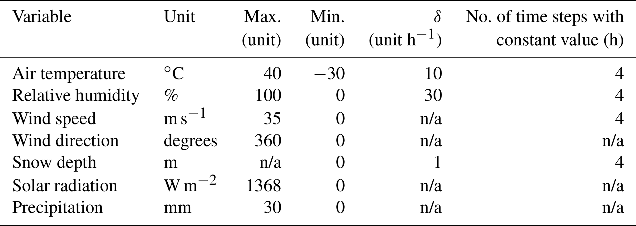
Measured weather data include air temperature (∘C), relative humidity (%), rain (mm), total precipitation (mm), snow depth (m), wind speed (m s−1), wind direction (∘), and incoming solar radiation (W m−2). Quality assurance procedures involved a combination of visual and automated inspection of the data for inconsistencies, such as sudden large increases in measurements, and outliers. Table A3 details the thresholds used to identify outliers and inconsistencies in the data. All data, except for the snow depth data, were gap-filled using linear regression from nearby station data. For instances when air temperature readings were faulty, relative humidity (RH) was first converted to vapour pressure and was then converted back to RH based on the appropriate temperature from the nearest station showing the greatest coefficient of determination.
Precipitation data required additional quality assurance procedures due to errors introduced by wind. Suspect spikes in rain intensity caused by wind-induced tips were identified through visual inspection initially but, starting from February 2016, were then done through an automated method. When three or more tips occurred within a 5 s scan interval, the data were flagged, assuming that three or more tips within 5 s would yield an extremely unlikely rainfall rate for the area (> 200 mm h−1). All suspect tips were removed and gap-filled. In addition, hourly rain data from WSN626, WSN693_703, WSN703_708, WSN819_1015, Hecate, East Buxton, SSN693, and Reference Station and hourly total precipitation data from East Buxton and Reference Station were corrected for undercatch (Yang et al., 1998) using the wind speed adjustment from Legates et al. (2005). This adjustment includes a station height variable, thus accounting for potential effects of the elevated total precipitation gauges at East Buxton and Reference Station and the rain gauge orifice at East Buxton (i.e., 4 m instead of 2 m). Please note that the precipitation data at the 5 min time step were not corrected for undercatch, as wind data at the 5 min level introduced too much noise to the corrected dataset. Further on, spikes in the snow depth data (> 1 m) that did not correspond to increases in total precipitation were removed and gap-filled, but gaps that were caused by sensor failures were generally too large and were therefore not filled.
3.2.2 Streamflow data
Stage data were quality controlled and flagged by visual inspection. Any spikes, drops, or changes in stage not associated with a rain event were further inspected and, where necessary, manually flagged and corrected. As an example, time lapse photos were used to confirm debris blockages to explain and correct unexpected small fluctuations in stage. Data gaps of < 30 min were filled using linear interpolation (computer automated), while gaps of > 30 min were filled using a relation (linear regression) between data from the backup, standalone water level sensors and pressure transducers. In the one exceptional case where both water level sensors were malfunctioning at watershed 819 (1 December 2015–17 May 2016), the stage records of watershed 844, the neighbouring watershed sharing many catchment characteristics, were used to estimate the stage by linear regression.
Discharge measurement uncertainties were calculated using the interpolated variance estimator (Cohn et al., 2013) for the velocity area method, which estimates uncertainty from the fluctuations in the flow velocity and depth profile and from calibration errors in the width, depth, and velocity measurements. Uncertainty estimations for the automated salt solution discharge measurements were recorded in both a quantitative and a qualitative manner. First, a quantitative percent error was calculated by error propagation of the uncertainty in the volume of salt solution, the EC sensor resolution, and the salt solution electrical conductivity calibration factor (Korver et al., 2018). Measurements with uncertainties higher than 20 % were excluded from further analysis. Second, the EC data were assessed for noise and spikes caused by turbulence at high flows. Where possible, spikes were removed, and noisy data were smoothed. Measurements that contained EC readings so noisy that they could not be corrected were removed. As an example, peak flows at watershed 703 were not successfully measured due to extremely turbulent flow conditions and, hence, extremely noisy EC data. Last, an assessment of salt mixing conditions at the downstream EC sensor site was performed by comparing calculated discharge from the two EC sensors placed within opposing sides of the river. If the calculated discharge differed by more than 1 %, then mixing conditions were considered poor, and unless the measurement filled an essential gap in the stage-discharge rating curve, it was excluded from further analysis.
Each discharge measurement was paired with a time-averaged measurement of the stage (recorded every second for the duration of the measurement), and rating curves were plotted for each station using locally estimated scatterplot smoothing (LOESS) regression (Fig. 2). The span widths of the LOESS fits were visually assessed and selected. Between 5 and 50 new measurements were added to each station's rating curve every year. Measurements prior to and after high-flow events were analyzed for possible shifts in the rating curves; in the case of a shift, time lapse videos and photos taken during maintenance surveys were investigated to confirm a concurrent change in streambed morphology, and a new curve was applied to the discharge time series from the onset of the high-flow event. The curves were extrapolated to minimum and maximum stage of the 5-year stage time series, estimating a zero stage to equal zero flow and estimating maximum flow by extrapolating a power law equation fitted on the upper section of the rating curves.
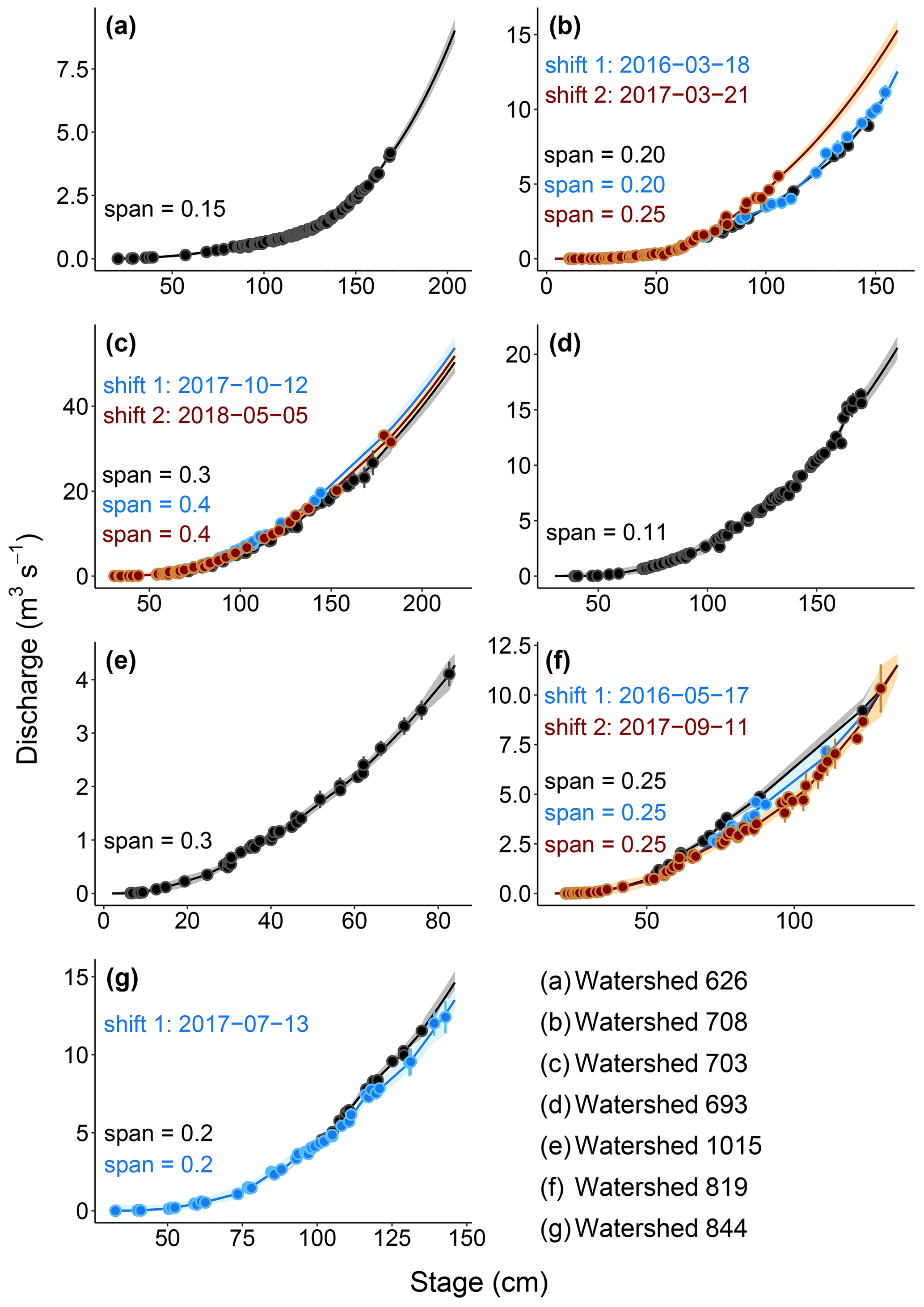
Figure 2Stage discharge rating curves, with 95 % confidence bands for the seven gauged watersheds. Large storm events caused rating curves to shift at some of the watersheds; dates are indicated for each individual shift. Rating curves were plotted using LOESS regression, and span widths (span) were visually selected for each individual curve.
Following the methodology proposed by Coxon et al. (2015), 95 % confidence intervals (CIs) were plotted around the rating curves in two steps. First, the absolute error of each stage discharge measurement was calculated by error propagation of the discharge measurement uncertainty (described above) and the stage measurement uncertainty. Stage measurement uncertainty was calculated as 2 times the standard deviation of the stage values recorded during the discharge measurement, so that measurements taken during rapidly falling or rising water levels were assigned higher uncertainties. The accuracy of the stage sensors used (±0.2 cm) was found to be inconsequential to the final calculation of discharge uncertainty, compared to flow turbulence and rapidly changing water levels. Second, CIs were derived from 500 curve fitting results of LOESS regressions on 500 randomized sets of stage discharge measurements and their maximum and minimum absolute measurement errors. For each millimetre of stage on the rating curve, 500 discharge values and 500 standard deviations were predicted and combined in a Gaussian mixed model to derive minimum and maximum absolute discharge (95 % CI). Any minimum absolute flow extending below zero was set to zero. Calculations were done in R, and the code has been made publicly available (Sect. 7). The output is a stage discharge lookup table with values of discharge, minimum discharge (95 % CI), and maximum discharge (95 % CI) for each millimetre of stage.
4.1 Weather and climate
The annual precipitation was 3246 mm (average of all stations within watershed boundaries); however, this may have been slightly underestimated as precipitation was measured as rain only, disregarding snow, at all but two locations (Table 2). Temperatures were generally mild, with mean annual temperatures of 8.2 ∘C ranging from monthly averages of 2.6 ∘C in December to 14.5 ∘C in August. Winter was characterized by intense windstorms (> 10 m s−1) from the southeast shifting to calmer winds from the south- and northwest in summer. Snowpacks were recorded at high elevations between December and May for all years and were persistent above 700 m a.s.l. and intermittent between 400 and 500 m a.s.l. However, weather conditions varied by season, year, location, and elevation, as described in more detail below.
Table 2Spatial variability of weather variables by meteorological station. Station names refer to stream sensor node (SSN) or weather sensor node (WSN), followed by the watershed ID, and are ordered by location (west to east on Calvert and then Hecate islands). Annual means (± standard deviation) were calculated for 2015/2016–2018/2019 water years. Values that are not indicated (–) are not measured at that specific station. Shown are mean annual precipitation (MAP)a, air temperature (MAT), wind speed (MAW), relative humidity (MARH), and snow depth (MASD). As MAP was measured as rain only at most stations, modelled precipitation with precipitation as snow (PAS), retrieved from ClimateNA (Wang et al., 2016) projections (2016–2019), is indicated for reference.
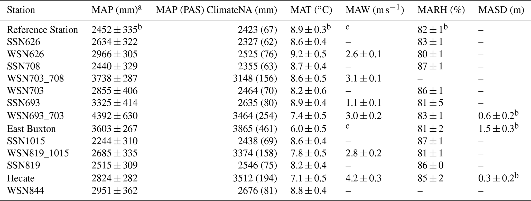
a Precipitation includes rain and snow measurements at Reference Station (∼ 5 % precipitation as snow) and East Buxton (∼ 30 % precipitation as snow) and was measured as rain only at all other stations where snowfall was assumed to be negligible. This was confirmed by the ∼ 5 % PAS at Reference Station and the ClimateNA model estimates of PAS never exceeding 5 %, except at East Buxton. b The period 2015–2016 was ignored due to data gap. c Data are available but have too many data gaps.
4.1.1 Spatial variations
Calvert Island received more precipitation (3353 mm yr−1) than Hecate Island (2676 mm yr−1). At low elevations (< 100 m a.s.l.), precipitation increased along a west-to-east gradient by about 120 mm km−1 on Calvert Island (R2=0.54, for stations between Reference Station and East Buxton) and 150 mm km−1 on Hecate Island (R2=0.88, for stations between SSN1015 and WSN844). Precipitation increased with elevation: about 70 mm per 100 m on Hecate Island (R2=0.26) and about 190 mm per 100 m on Calvert Island (R2=0.54). There was almost a 50 % increase in mean total precipitation between Reference Station on western Calvert Island (42 m a.s.l., 2452 mm) and East Buxton in the east (740 m a.s.l., 3603 mm), with 5 % versus 30 % falling as snow at the respective stations. The seasonal snowpack at East Buxton station reached an average maximum depth of 1.4 m, whereas intermittent snow cover records at lower elevation (WSN693_703; 449 m a.s.l.) and at the south-facing slope of Hecate Island (Hecate; 477 m a.s.l.) never exceeded 0.6 and 0.3 m, respectively.
Air temperature decreased with increasing elevation at a rate of approximately 0.35 ∘C per 100 m (−0.36 and −0.32 ∘C per 100 m on Calvert (R2=0.83) and Hecate (R2=0.87) islands, respectively), from 8.7 ∘C at sea level to 6.0 ∘C at 740 m a.s.l. This lapse rate varied seasonally, with small differences in temperature between low and high elevation stations during summer months (−0.1 ∘C per 100 m in August) and large differences in winter (−0.5 ∘C per 100 m in February). All stations recorded an average relative humidity (RH) between 80 % and 87 %, with high elevation stations reaching lower RH levels (e.g., minimum of 16 % daily RH at East Buxton) than low elevation stations (e.g., minimum of 37 % daily RH at SSN708). General wind directions were uniform across Calvert and Hecate islands, except for the areas around Mount Buxton which showed local variability. The highest wind speed was recorded at Hecate station (27.3 m s−1), which also recorded the highest wind speeds on average (4.4 m s−1), and station SSN693 was, despite being adjacent to a lake, the most sheltered (average of 1.1 m s−1). Station-specific annual weather parameters are summarized in Table 2.
4.1.2 Temporal variations
Seasonal variations in weather variables were analyzed for station SSN708, the station with the longest record (installed September 2013; 12 m a.s.l.), as a representative for the study region. There were wet (October–April) and comparatively dry (May–September) seasons, with the dry season starting abruptly in May but transitioning gradually into the wet season in September (Fig. 3). Although the average monthly rainfall was distinctly lower in the dry season (128 versus 320 mm in the wet season), rain events still regularly occurred; the longest dry periods never exceeded between 9 and 11 consecutive days, usually in July or August. The wet seasons were marked by large intermonthly and interannual variations (58–524 mm per month), whereas variations were comparatively small during the dry seasons (22–218 mm per month). November was the wettest and July the driest month of the year (average of 362 and 78 mm, respectively). Frequently recurring high wind storms (> 10 m s−1) from a predominantly southeasterly direction characterized the wet season, and low northwesterly and southwesterly winds (< 10 m s−1) prevailed during the dry season (Fig. 4), averaging each year to 2.7 m s−1. Monthly average air temperature followed an annual cycle ranging between 2.2 ∘C in February and 14.5 ∘C in August, with overall elevated midwinter temperatures recorded in January (4.3 ∘C). This seasonal trend was consistent between years, except for the month of February, which varied markedly from year to year (between −0.8 and 7.6 ∘C). Like air temperature, relative humidity followed an annual cycle, peaking in August (90 %) and reaching a low in February (85 %), with relatively more year-to-year variability in winter.
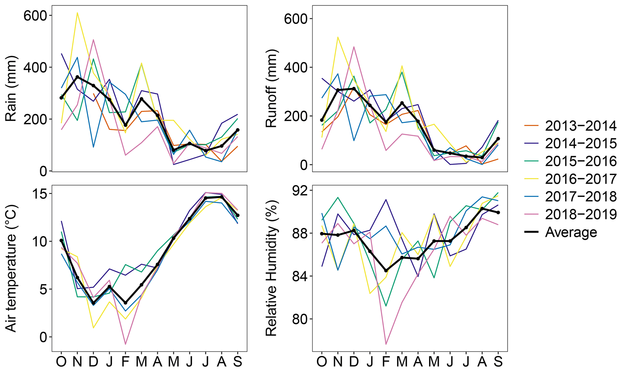
Figure 3Seasonal rain, runoff, air temperature, and relative humidity by water year. Monthly totals (rain and runoff) and monthly averages (air temperature and relative humidity) from station SSN708 are shown, as it is the station with the longest record (installed September 2013; 12 m a.s.l.).
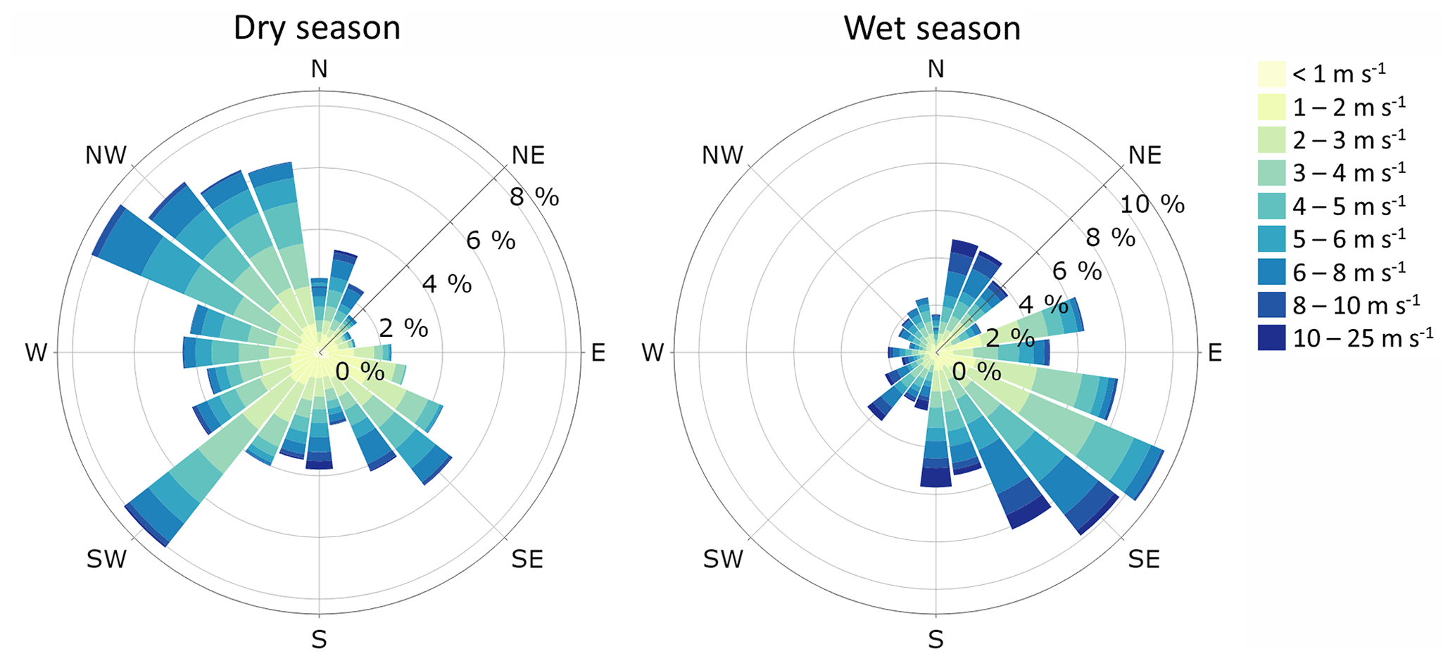
Figure 4Average hourly wind speeds and wind directions during the dry (May–September) and the wet (October–April) meteorological seasons. The frequency of occurrence is indicated in percent of time for the entire measurement record of Hecate station (October 2015–October 2019).
Between water years, average precipitation and air temperature varied, whereas wind speed and relative humidity were consistent (2.7 m s−1 and 82 %–84 %). Water year 2016–2017 was, within the short record period, relatively wet and cool (7.6 ∘C; 3681 mm), whereas 2018–2019 was drier than average (2770 mm; Table 3). Maximum air temperature was recorded in September 2016 (30 ∘C; SSN693) and minimum air temperature in February 2019 (−16.3 ∘C; East Buxton). Snowfall was highest in the winter of water year 2017–2018 and lowest in 2015–2016, with maximum snow depths measuring 1.8 and 0.2 m, respectively, at East Buxton. Maximum snow accumulation was usually reached in March.
Table 3Annual variability in precipitation, runoff, maximum snow depth, and mean air temperature (by water year; 1 October–30 September). Runoff was averaged over all seven watersheds and scaled by watershed area. Precipitation and air temperature were averaged over all meteorological stations, except for Reference Station (no data 2015–2016). The period 2014–2015 was not calculated because stations WSN6226 and WSN844 had not been installed yet. Maximum snow depth was determined from daily aggregated values of 3 h moving averages. NA represents not available.
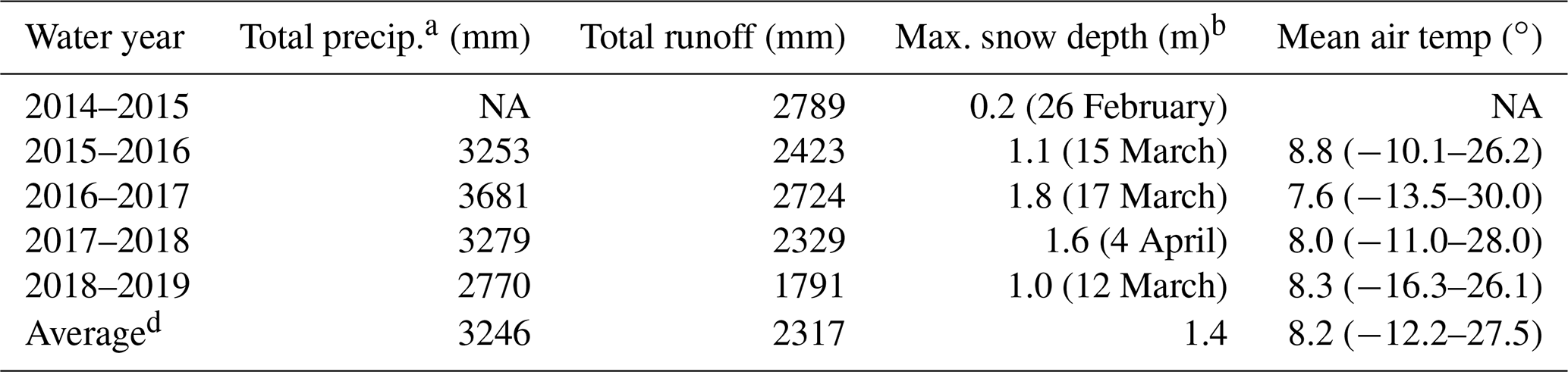
a An underestimate because all stations, except for East Buxton, only measure rain, not rain and snow. b Measured at East Buxton (740 m a.s.l.). c Measured at Hecate station. d Averaged over water years 2015–2016 to 2018–2019.
4.2 Streamflow and catchment processes
The average yearly runoff from all watersheds, scaled by watershed area, was 2317 mm, suggesting that ∼ 30 % of precipitation (3246 mm) was not accounted for in surface runoff. The average flux of freshwater from the seven watersheds was 0.1087 km3 yr−1. Seasonal runoff patterns followed the wet (October–April) and comparatively dry (May–September) patterns of rainfall, with runoff dropping abruptly in May but increasing gradually into the wet season in September and reaching the highest flows in November and December (Fig. 3). Runoff generated in the wet season accounted for 84 % of the total average yearly runoff.
Freshwater fluxes were dominated by large storm events, where 34 % of all freshwater delivered to the ocean occurred during very high flows that were only exceeded for 5 % of the record (≥ P5 flows), and although none of the rivers fully ceased to flow during the record period, baseflows were low, with P95 flows approaching zero (Table 4). The majority (92 %) of the ≥ P5 flows occurred during the wet season, with 48 % occurring in November and December. In accordance, 98 % of all days with very low flows (≤ P95) occurred during the dry season, of which 52 % occurred during the month of August. Storm events resulted in rapid streamflow responses: average lag times (the time from peak rain to the start of rise in streamflow) were less than 8 h for most watersheds, and average peak times (the start of rise in streamflow to peak discharge) were generally under 12 h (Table 4). The variation in runoff responses across the study area is illustrated by Fig. 5, which shows a hydro-hyetograph of a large rainstorm which produced 114 mm over 3 d and reached the highest rain intensity (74 mm in 24 h) on 16 October 2017. Discharge peaked at 50 and 20 m3 s−1 at watersheds 703 and 693 but never exceeded 12 m3 s−1 in the other rivers. This can only be partially explained by differences in watershed size; those watersheds draining large lakes (1015 and 708) or a chain of lakes (693) had relatively subdued peak flows and longer-lasting receding limbs. In addition, whereas peak flows generally showed a positive relation to watershed size, high flow values (P5) of watersheds 708 and 1015 were subdued compared to similar or smaller-sized watersheds (Table 4). Furthermore, lag times and peak times of watersheds 1015 and 693 (∼ 20 and ∼ 25 h) were much higher than those of the other watersheds, including watershed 708; this can be explained by the relatively small contributing watershed area upstream of watershed 708's large lake, whereas the lakes at watersheds 1015 and 693 are located close to the watershed outlets.
Table 4Hydrometeorological characteristics of the seven gauged watersheds. Shown are mean annual total precipitation (MAP)a, runoff (MAR), and streamflow (MASF) averaged over the water years with complete precipitation station records (October 2015–October 2019). Additional metrics include the flow duration exceedance probabilities for low (P95) and high (P5) flows, the percent of annual runoff originating from > P5 events, the percent of uncertainty in annual runoff, the mean lag and peak times (time from peak rain to start of rise in hydrograph and start of rise in hydrograph to peak discharge, respectively)b, and the runoff coefficient (MAR/MAP). Total precipitation was averaged over the records of the stations located inside and at the border of each watershed. Averages for watersheds 693 and 703 also include measurements from East Buxton, which is located outside the watershed boundaries but close enough to be representative of the watersheds' high elevation areas. Climate normals (1981–2010) for precipitation with precipitation as snow (PAS) were calculated by averaging station-specific, modelled ClimateNA data (Wang et al., 2016).

a Annual precipitation is calculated from rain and snowfall measurements at watersheds 693 and 703 (including total precipitation from East Buxton) but from rainfall measurements only at the other lower elevation watersheds where snowfall was assumed to be negligible. This was confirmed by the ∼ 5 % PAS at Reference Station (42 m a.s.l.; outside watershed boundaries) and the ClimateNA model estimates of PAS never exceeding 5 % (see Table 2 for station-specific PAS model estimates). b Calculated from 50 rain events of varying sizes that started from baseflow conditions and had single peak flows in all rivers that occurred throughout the record period during both wet and dry seasons.
Variations in discharge volume and streamflow responses among the seven watersheds can be explained by watershed characteristics but also by the spatial variation in precipitation (Sect. 4.1.1). For example, although freshwater fluxes (total volume) were directly related to watershed size, runoff (area-scaled yields) varied greatly between 1502 and 3066 mm yr−1 for watersheds 1015 and 693, respectively, showing a clear spatial pattern of increasing runoff from west to east, with lower overall runoff on Hecate Island. These patterns mirror those of rain and total precipitation, where inputs vary between 2465 and 3774 mm yr−1 at watersheds 1015 and 693, respectively. Potential factors that contributed to these differences include the presence of Mount Buxton, which resulted in elevated precipitation lapse rates on eastern Calvert Island, the high occurrence of large storm events, with wind directions from the southeast potentially causing a rain shadow from Mount Buxton, and the steep relief, exposed bedrock, and sparsely vegetated and shallow soils at high-elevation areas of Mount Buxton contributing to rapid runoff generation and elevated runoff coefficients of 77 % and 81 % (versus 60 % to 66 % for the other watersheds; Table 4).
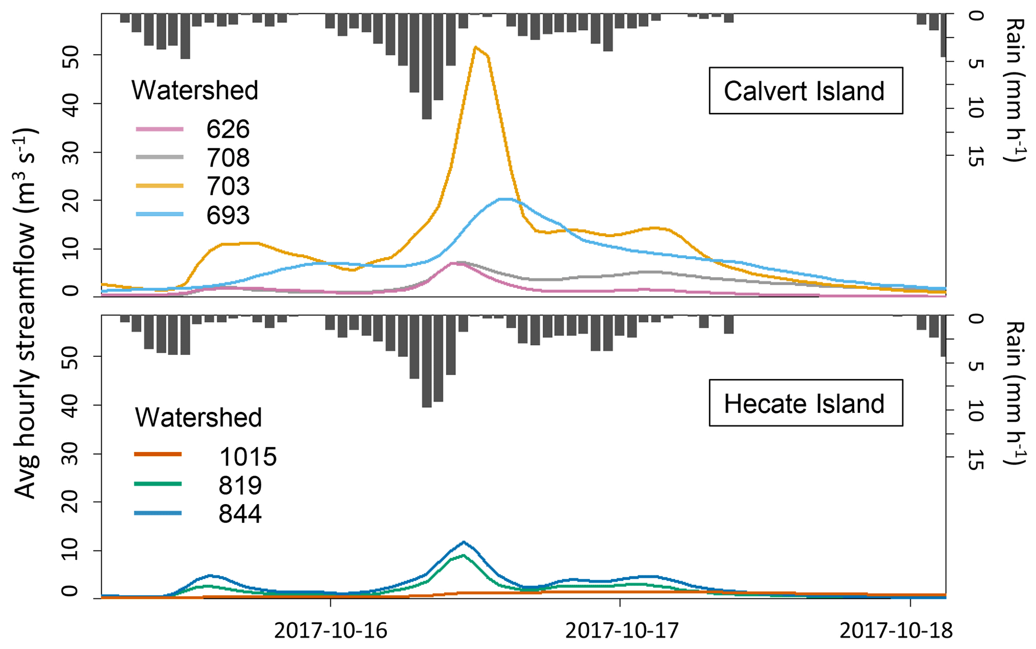
Figure 5Hydro-hyetographs for the seven gauged watersheds during a large storm event (114 mm of rain in 3 d). Rain measurements at SSN708 and SSN819 are shown.
A muted freshet from seasonal snowpacks contributed to streamflow in watersheds 703 and 693. Visual inspection of the hydrograph of watershed 703 showed daily fluctuations of streamflow during dry conditions from April to June, with peak flows occurring ∼ 12 h after maximum daily air temperature (Fig. A3). These streamflow fluctuations were, compared to peak flows after rainfall events, small (increases of a maximum of 0.2 m3 s−1 versus up to 1 to 40 m3 s−1 during rain events) and could not be distinguished during rainy periods, suggesting that snowmelt made up a small component of annual runoff generation. However, the Mount Buxton snowpack has the potential to contribute to peak flows during rain-on-snow events, especially in watersheds 703 and 693 and, to a lesser extent, 708.
Based on the general climatic conditions and hydrographs, these watersheds have rainfall-dominated (pluvial) streamflow regimes with peak flows occurring from the early fall through to midwinter and low flows in the summer months (Moore et al., 2012). This contrasts to the freshwater fluxes from one of the major drainage basins within the larger study area, i.e., the Wannock River catchment (3900 km2, ∼ 50 km east of Calvert Island), which has a snow- (nival) and glacial-melt-dominated regime, with the highest sustained flows in the summer months. Total Wannock River freshwater fluxes reached, on average, 9.5742 km3 yr−1, which is around a factor of 100 higher than the fluxes from the seven watersheds on Calvert and Hecate islands combined (0.1087 km3 yr−1). However, yields (scaled by watershed size) were comparable (2317 vs. 2455 mm; Wannock River daily discharge data, 2021). Despite these major differences in flow regimes, Wannock River peak flows generally occurred in the late fall and early winter when atmospheric rivers make landfall (Wannock River annual instantaneous extreme discharge data, 2021; Sharma and Déry, 2019). These atmospheric rivers, combined with warm temperatures and strong winds, can melt early season snow and glaciers at higher elevations. It is during such storms that freshwater discharge was likely synchronized across the region, with corresponding high material flux to the marine ecosystems. It is expected that current yields and streamflow regime will change due to accelerated glacial loss in the Wannock basin (Menounos et al., 2019), a projected increase in the region's mean annual precipitation, with less falling as snow (Shanley et al., 2015), and more frequent and intense atmospheric river events (Déry et al., 2009).
5.1 Uncertainties in the weather data
Rainfall data that were corrected for wind-induced undercatch were, on average, 12 % greater than the raw data. The largest corrections were applied at WSN693_703 (13 %), which was exposed to some of the highest recorded wind speeds. In contrast, station SSN693 was at a much lower elevation with lower exposure, resulting in overall corrections of 7 %. Some stations exposed to wind required additional anchoring and thus had increased uncertainty due to wind-induced tips between 2014 and 2018 (WSN693_703, WSN703_708, and Hecate). This was corrected using a tip threshold (> 3 tips per 5 s) to remove faulty tips. However, it was difficult to discern whether some of these tips represented real events, even when using adjacent stations as comparison. Following proper anchoring in 2018, 1 % to 2 % of the annual rainfall record was flagged as suspect and cleaned. Tipping bucket calibrations indicated that there were no shifted values over the course of the study period, but site-specific issues with tipping buckets included blown-off lids (WSN703_708), blockages from debris (WSN703 and WSN844), and wiring damage by wolves causing false tips (819_1015). Obvious spikes in the snow depth data, caused by heavy snowfall and wind, were corrected, but large data gaps due to sensor failures were not filled. It should be noted that the SR50 snow depth sensors had a high rate of failure (1 to 2 years), and thus, sensors were replaced annually. The anemometers occasionally froze in winter, causing wind direction records to become stuck. However, these issues were usually short lived, as the sensors would melt during the daytime.
The majority of weather stations only measured rainfall and not snow (12 out of 14 stations; Table A1), and thus, there was likely an underestimation of precipitation across the study area. All stations above 400 m a.s.l. measured snow depth to assess the relative contribution of snow, but these data were not used to correct rainfall at these locations. However, according to ClimateNA modelled data, snow made up less than 5 % of annual precipitation at all stations (except East Buxton at 740 m a.s.l.), including those between 400 and 500 m a.s.l. It is therefore likely that any errors associated with not measuring total precipitation at all sites is less than the variation in precipitation across the study area.
5.2 Uncertainties in the streamflow data
Streamflow measurements are affected by many sources of uncertainty, and thus, it is important to both identify and quantify these errors. One potentially major source of error which can be difficult to quantify is the lack of high-flow discharge measurements necessitating the extrapolation of a rating curve from the highest measured flow up to the highest measured stream stage (Coxon et al., 2015; Domeneghetti et al., 2012). However, the automated salt dilution measurement system enabled the collection of hundreds of measurements taken along the near-full range of stage values in the rating curve for most of the watersheds, therefore allowing us to quantify discharge uncertainty generally not reported.
Channels were stable in watersheds 626, 693, and 1015 for the duration of the data presented, but large storm events resulted in rating curve shifts in watersheds 708, 703, 819, and 844. These watersheds all experienced one to two rating curve shifts within the 5-year data record (Fig. 2). However, the automated salt dilution measurement method allowed regular and ample discharge measurements before and after big storms, and thus, shifts could be tracked with minimal rating curve data gaps. In addition, peak flows were measured at the upper end of the rating curve in most watersheds. For all watersheds, less than 0.12 % of discharge data points were calculated from the extrapolated part of the rating curve; in other words, fewer than 2.5 d of the 5-year discharge time series are estimated and not measured. On a volumetric basis, between 1 % and 3 % of total water discharge from watersheds 626, 693, and 819 was calculated from the extrapolated parts of rating curves and below 1 % for all other watersheds.
Despite having discharge measurements for the majority of stage measurements in the rating curves, there was significant error in the discharge dataset presented, with mean annual runoff from the seven watersheds potentially being overestimated by 24 % and underestimated by 43 %. Uncertainty varied by watershed (Table 4), with the amounts depending on the spread and measurement uncertainties of individual discharge data points at different positions along the rating curves (affecting the widths of confidence bands). Underlying causes were related to channel stability, turbulence, downstream mixing of salt solution, and general uncertainties introduced by equipment accuracies, which are described in more detail below.
Discharge measurement error was always below 20 % at low flows and generally under 5 % but occasionally no more than 15 % at high flows when using the automated salt dilution method. The largest factor contributing to the uncertainty of low-flow measurements using the velocity area method was the uncertainty in the velocity readings. Despite careful selection of river cross-section sites, ideal sites with minimal flow velocity variation were sparse due to the rivers' steep gradients and complex streambeds. The largest factor contributing to the salt dilution measurement uncertainty was the error associated with the salt solution electrical conductivity calibration factor, which was sensitive to the salt solution's mixing prior to transfer, temperature, and the precision of the calibration equipment (∼ 70 % of total measurement error). The next largest factor was the error associated with determining the salt solution dump volume, which, due to the system being automated, had to be determined indirectly from pressure measurements (using a pressure transducer inside a stainless-steel collector) and could therefore vary with salinity and within the limits of sensor accuracy. This uncertainty increased with decreasing volume (∼ 30 % of total measurement error). Further on, the discharge measurement error was increased by incomplete mixing of salt solution or excessive noise in the EC data at downstream sensors. However, most measurements affected were removed from further analysis, except for measurements at the upper end of the rating curves where no other data were available (e.g., high flows at watersheds 703 and 1015, reaching up to 15 % measurement uncertainty).
Selecting a stage value to match a discharge measurement for rating curve plotting was difficult when flows were either turbulent and/or the stream level was rapidly rising or falling during the discharge measurement. This error was quantified by propagating the standard deviation of stage values recorded during a discharge measurement to total discharge uncertainty. Fluctuating stage values were mostly a concern for high-flow measurements at watershed 819, where stage values could be noisy and rapidly increase or decrease within a 5 to 15 min measurement interval, increasing discharge measurement uncertainties by, on average, 2 % (range of 0 % to 9 %). This was also a concern at watershed 844 but to a lesser magnitude (uncertainty increases of 0 % to 3 %). All other watersheds were only minorly affected (typically < 1 %).
Rating curve confidence intervals are narrow, resulting in low overall discharge uncertainty, if (1) discharge measurement uncertainties are low and (2) there is little spread in the rating curve data points. These conditions were met for watersheds 626 and 708, resulting in an overall uncertainty in the yearly runoff of % (lower CI) and +23 % (higher CI; Table 4, Fig. 2). The rating curves of watersheds 703 and 1015 were of high quality at low- to mid flows, but the confidence intervals widened above 15 and 1 m3 s−1, respectively, because of increased measurement uncertainties related to incomplete salt solution mixing at the downstream sites. Measurements taken at watershed 693 all had low uncertainties (< 5 %, except at very low flows), but nonetheless, a spread in the data (> 3 m3 s−1) increased the confidence intervals, suggesting that there were sources of error unaccounted for in the quantitative uncertainty estimations. Measurements taken at mid- to high flows at watersheds 819 and 844 (> 4 and 5.5 m3 s−1, respectively) had the highest uncertainty due to incomplete salt mixing at the downstream EC sensors and a rapidly fluctuating stage during high flows. In addition, unstable channel conditions at watershed 819 caused a rating curve shift once per year, and in some instances, the complete rating curve could not be rebuilt before the next shift. All the above issues resulted in an overall uncertainty in the yearly runoff of % (lower CI) and % (higher CI) for watersheds 844 and 819, respectively.
All discharge and weather data presented in this paper are available at https://doi.org/10.21966/J99C-9C14 (Korver et al., 2021), and watershed delineations with watershed metrics can be found at https://doi.org/10.21966/1.15311 (Gonzalez Arriola et al., 2015). Both data packages include a Readme file detailing the data file content and contact information for further details.
Calculations were done in R. The rating curve script is available at https://doi.org/10.5281/zenodo.7043719 (Korver, 2022) and the scripts used for weather data quality control can be found at https://doi.org/10.5281/zenodo.7044487 (Haughton, 2022).
The hydrometeorological data of the Kwakshua Watersheds Observatory fills a critical data gap on the outer coast of the northeast Pacific coastal temperate rainforest (NPCTR) of North America and over time will help us to better understand the hydrology of the region. The hydrometeorological dataset presented is part of a greater interdisciplinary effort to better understand this region, including oceanography, biodiversity, ecology, climate, and watershed processes. High-quality data are assured using state-of-the-art technology and thorough data quality procedures. Discharge data presented here are unique because the novel method of measuring streamflow accounts for measurement error from various sources, which is often not quantified in publicly available datasets. The dataset also highlights the difficultly of measuring streamflow in small, turbulent streams and identifies key sources of uncertainty which should be included when using these data for analysis and modelling.
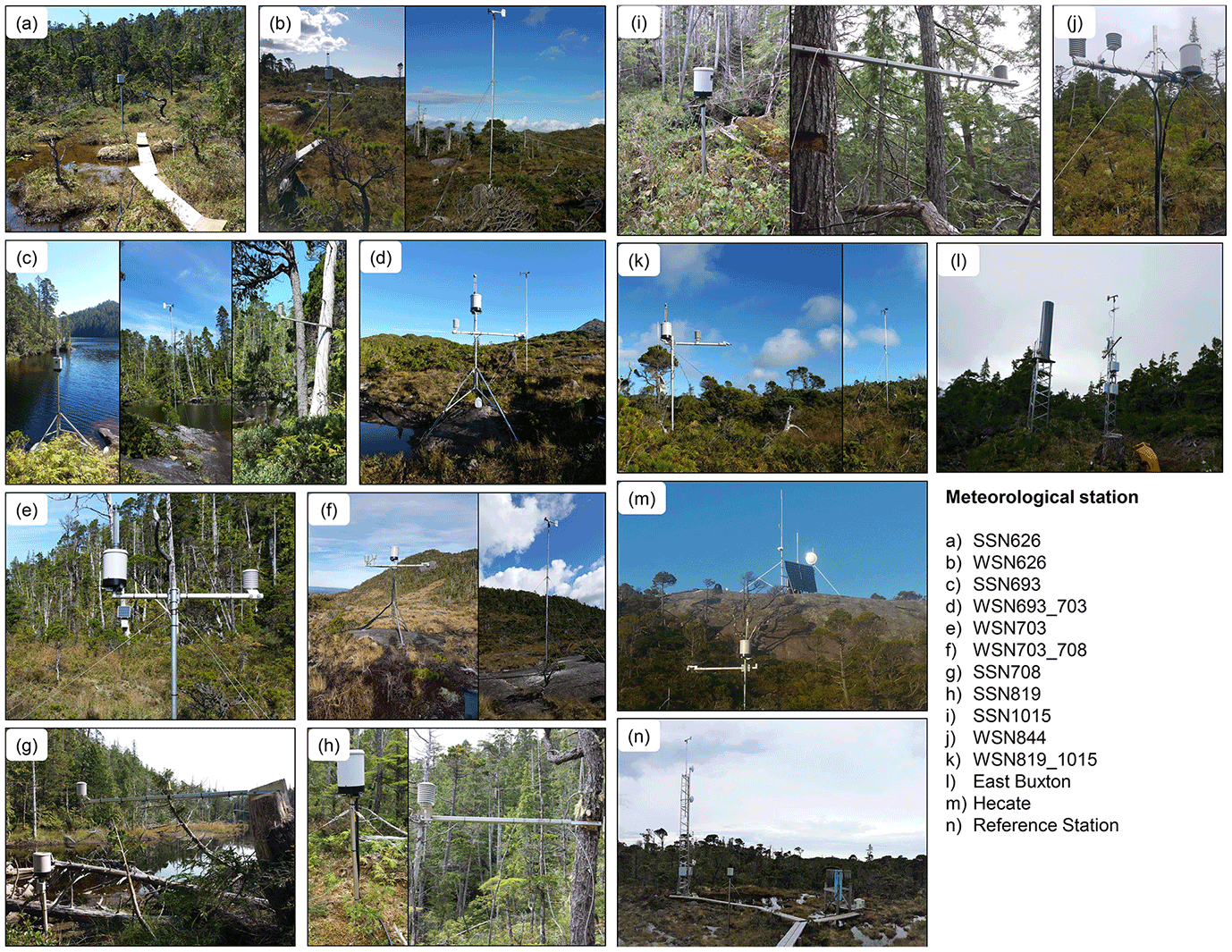
Figure A1Images of the meteorological stations. Photos by Shawn Hateley and Bill Floyd.

Figure A2Images of the seven streams near the watershed outlets. Shown are the water level gauging site (watershed 693), the downstream sites of the automated salt-in-solution discharge measurement method (watersheds 703 and 1015), and the upstream sites of the automated salt-in-solution discharge measurement method with dumping mechanism (all other watersheds). Photos by Shawn Hateley, Bill Floyd, and Maartje Korver.
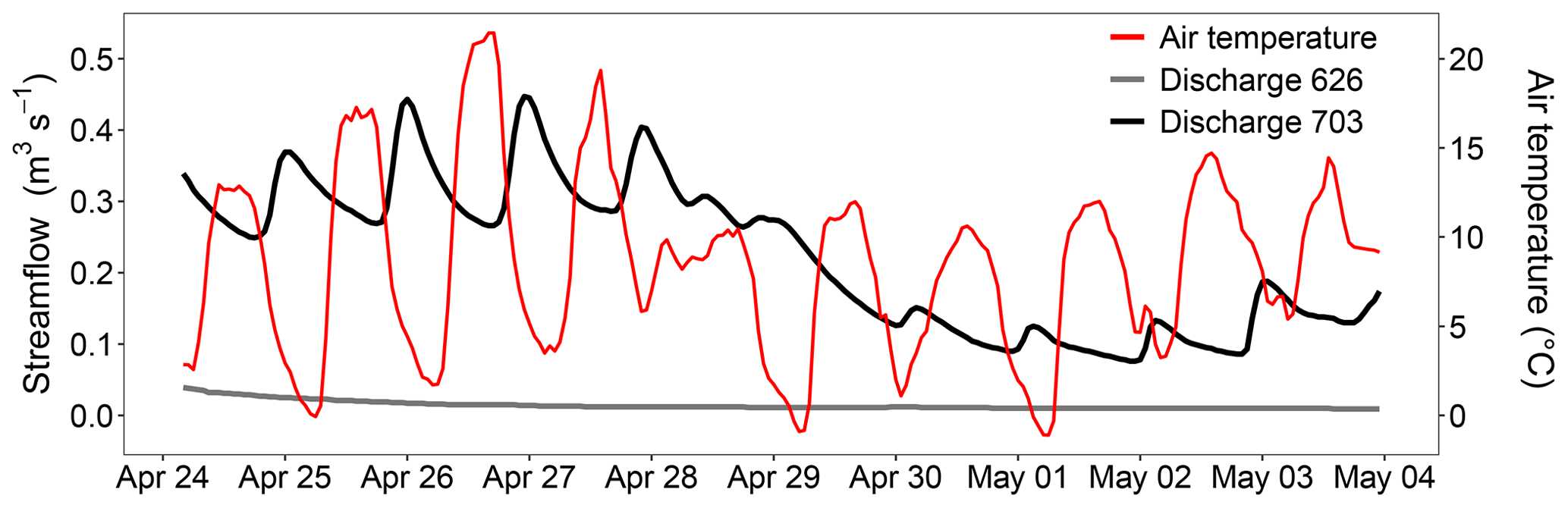
Figure A3Discharge and air temperature at watershed 703 during 10 d without rainfall in the snowmelt season (measured at SSN703 and WSN703, respectively). Daily fluctuations in 703's streamflow indicate snowmelt contributions. Peak flows occur ∼ 12 h after the daily maximum air temperatures. Discharge at watershed 626 (low elevation watershed with no snowpack) is shown for reference. The stable recession indicates no rainfall inputs during this period.
Table A1Station location and installation details. Station names refer to stream sensor node (SSN) or weather sensor node (WSN), followed by the watershed ID, and are ordered by location (west to east on Calvert and then Hecate islands). Reference Station and East Buxton are located outside watershed boundaries and Hecate is located at the boundary of watersheds 819 and 844 (Fig. 1).
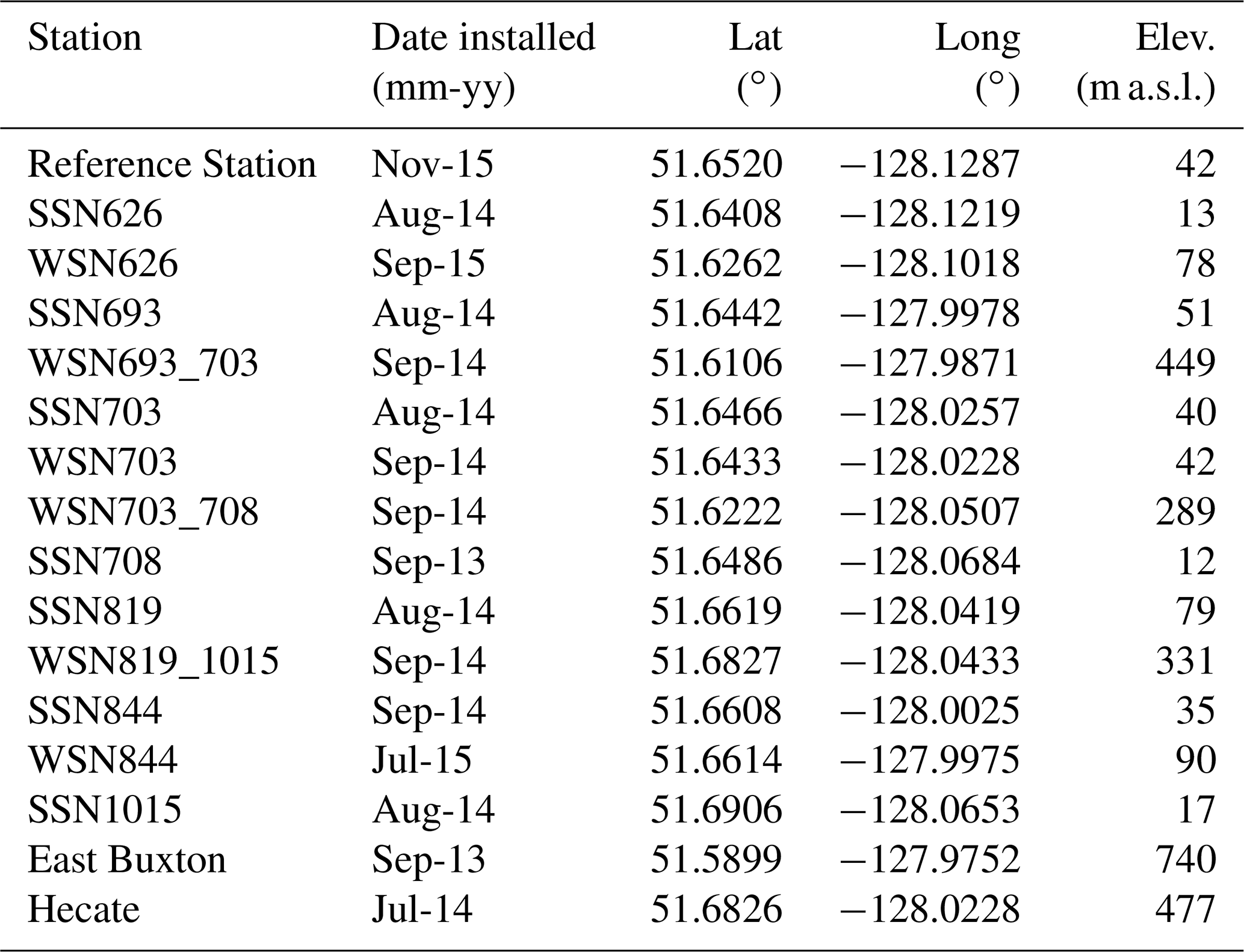
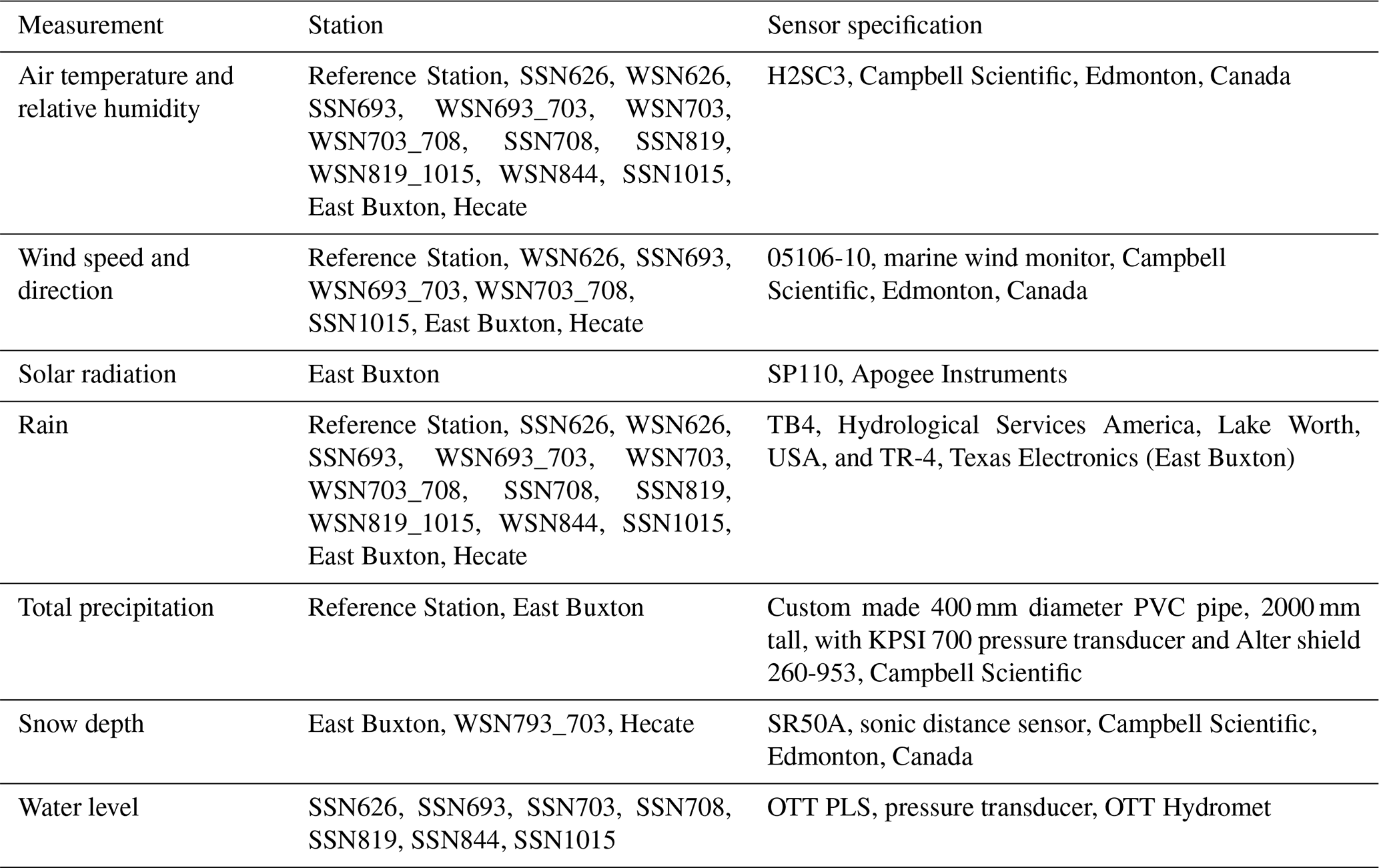
Table A3Thresholds used to instigate quality control procedures of the weather data, with the maximum and minimum values, a maximum rate of change (δ), and the maximum number of time steps with a constant value. Outlier data were flagged or, where necessary, corrected and gap-filled. n/a represents not applicable
MCK wrote the paper, with contributions from EH for the meteorology sections and overall contributions from WCF and IJWG. WCF designed the hydrometeorological station network and was responsible for installation and maintenance. MCK and EH managed, quality controlled, and conducted analysis on the streamflow and weather data, respectively, with supervision from WCF. Data collection, station installation, and maintenance was performed by WCF, MCK, and EH, among many others specified in the acknowledgements. IJWG led the watershed characterization in addition to co-conceptualizing and co-designing the broader Kwakshua Watersheds Observatory, along with WCF and others (see the acknowledgements).
The contact author has declared that none of the authors has any competing interests.
Publisher's note: Copernicus Publications remains neutral with regard to jurisdictional claims in published maps and institutional affiliations.
We gratefully acknowledge that this work was conducted on the traditional, ancestral, and unceded territories of the Haíłzaqv and Wuikinuxv Nations. We would like to sincerely thank the Hakai Institute support staff involved in operating the Kwakshua Watersheds Observatory. The installation and development of this observatory arose from research ideas first conceived by Ken Lertzman, who still acts as a primary scientific advisor. In addition, Ilja van Meerveld supervised the early stages of the development of the discharge measurement and uncertainty calculation methods. Ray Brunsting was, as head of IT, a key person in the early days of the observatory design, and he continues to aid in the management and quality assurance of the data. Hakai Energy Solutions, specifically Colby Owen and James McPhail, have been indispensable in designing, data-logger programming, and installing the extensive telemetry network enabling real-time data access. Shawn Hateley has led many field maintenance operations, and Stewart Butler has been responsible for the maintenance of the salt dilution systems. GIS calculations of watershed characteristics were done by Santiago Gonzalez Arriola. Many people assisted with the installation and maintenance operations, including Will McInnes, Jason Jackson, Rob White, Isabelle Desmarais, David Norwell, Christopher Coxson, Christian Standring, Libby Harmsworth, Ben Millard-Martin, Carolyn Knapper, Midoli Bresch, Parker Christensen, Andrew Sharrock, Darren Cashato, Michel Stitger, Mike Mearns, Dave Snow, Nelson Roberts, Lawren McNab, Ondine Pontier, Eric Courtin, and Hannah McSorely.
This research has been supported by the Tula Foundation, the Ministry of Forests, Lands, Natural Resource Operations and Rural Development and Environment and Climate Change Canada.
This paper was edited by Sibylle K. Hassler and reviewed by two anonymous referees.
Alaback, P. B.: Biodiversity patterns in relation to climate in the temperate rainforests of North America, in: High latitude rain forests of the west coast of the Americas: climate, hydrology, ecology and conservation, edited by: Lawford, R., Alaback, P. B., and Fuentes, E. R., Ecological studies, Springer, Berlin, 113, 105–133, 1996.
Arriola, S. G. and Holmes, K.: Hakai Terrain Relief, Hakai Geospatial data, ArcGIS Online [data set], http://hakai.maps.arcgis.com/home/item.html?id=711527c3469a4012bd0b25983de4b3d9 (last access: 16 September 2020), 2017.
Banner, A., LePage, P., Moran, J., and de Groot, A. (Eds.): The HyP3 Project: pattern, process, and productivity in hypermaritime forests of coastal British Columbia – a synthesis of 7-year results, B.C. Min. For., Res. Br., Victoria, B.C. Spec. Rep., 10, https://www.for.gov.bc.ca/hfd/pubs/docs/srs/Srs10.htm (last access: 10 January 2021), 2005.
Bidlack, A. L., Bisbing, S. M., Buma, B. J., Diefenderfer, H. L., Fellman, J. B., Floyd, W. C., Giesbrecht, I., Lally, A., Lertzman, K. P., Perakis, S. S., Butman, D. E., D'Amore, D. V., Fleming, S. W., Hood, E. W., Hunt, B. P. V., Kiffney, P. M., McNicol, G., Menounos, B., and Tank, S. E.: Climate-Mediated Changes to Linked Terrestrial and Marine Ecosystems across the Northeast Pacific Coastal Temperate Rainforest Margin, BioScience, 71, 581–595, https://doi.org/10.1093/biosci/biaa171, 2021.
Cohn, T. A., Kiang J. E., and Mason Jr., R. R.: Estimating Discharge Measurement Uncertainty Using the Interpolated Variance Estimator, American Society of Civil Engineers, https://doi.org/10.1061/(ASCE)HY.1943-7900.0000695, 2013.
Coxon, G., Freer, J., Westerberg, I. K., Wagener, T., Woods, R., and Smith, P. J.: A novel framework for discharge uncertainty quantification applied to 500 UK gauging stations, Water Resour. Res., 51, 5531–5546, https://doi.org/10.1002/2014WR016532, 2015.
Déry, S. J., Stahl, K., Moore, R. D., Whitfield, P. H., Menounos, B., and Burford, J. E.: Detection of runoff timing changes in pluvial, nival, and glacial rivers of western Canada, Water Resour. Res., 45, W04426, https://doi.org/10.1029/2008WR006975, 2009.
Domeneghetti, A., Castellarin, A., and Brath, A.: Assessing rating-curve uncertainty and its effects on hydraulic model calibration, Hydrol. Earth Syst. Sci., 16, 1191–1202, https://doi.org/10.5194/hess-16-1191-2012, 2012.
Ecotrust, Pacific GIS, & Conservation International: Original distribution of the Coastal Temperate Rain Forest, in: The rainforests of home: An atlas of people and place, Interrain, Portland, Oregon, https://ecotrust.org/wp-content/uploads/Rainforests_of_Home.pdf (last access: 15 February 2021), 1995.
Fang, X., Hou, X., Li, X., Hou W., Nakaoka, M., and Yu X.: Ecological connectivity between land and sea: a review. Ecol Res 33, 51–61, https://doi.org/10.1007/s11284-017-1549-x, 2018.
Fiedler, F. R.: Simple, practical method for determining station weights using Thiessen polygons and isohyetal maps, J. Hydrol. Eng., 8, 219–221, https://doi.org/10.1061/(ASCE)1084-0699(2003)8:4(219), 2003.
Giesbrecht, I. J. W., Floyd, W. C., Tank, S. E., Lertzman, K. P., Hunt, B. P. V., Korver, M. C., and Del Bel Belluz, J.: The Kwakshua Watersheds Observatory, central coast of British Columbia, Canada, Hydrol. Process., 35, e14198, https://doi.org/10.1002/hyp.14198, 2021.
Giesbrecht, I. J. W., Tank, S. E., Frazer, G. W., Hood, E., Gonzalez Arriola, S. G., Butman, D. E., D'Amore, D.V., Hutchinson, D., Bidlack, A., and Lertzman, K. P.: Watershed classification predicts streamflow regime and organic carbon dynamics in the Northeast Pacific Coastal Temperate Rainforest, Global Biogeochem. Cy., 36, e2021GB007047, https://doi.org/10.1029/2021GB007047, 2022.
Gonzalez Arriola, S., Frazer, G. W., and Giesbrecht, I.: LiDAR-derived watersheds and their metrics for Calvert Island, Hakai Data Catalogue [data set], https://doi.org/10.21966/1.15311, 2015.
Gonzalez Arriola, S., Giesbrecht, I. J. W., Biles, F. E., and D'Amore, D. V.: Watersheds of the northern Pacific coastal temperate rainforest margin, Hakai Data Catalogue [data set], https://doi.org/10.21966/1.715755, 2018.
Green, R. N.: Reconnaissance level terrestrial ecosystem mapping of priority landscape units of the coast EBM planning area: Phase 3, Prepared for British Columbia Ministry Forests, Lands and Natural Resource Ops., Blackwell and Associates, Vancouver, Canada, 2014.
Haughton E.: wx-tools v1, Zenodo [code], https://doi.org/10.5281/zenodo.7044487, 2022.
Henshaw, D. and Martin, M.: Sensor Data Quality, https://wiki.esipfed.org/Sensor_Data_Quality (last access: 1 April 2021), 2014.
Hill, D. F., Ciavola, S. J., Etherington, L., and Klaar, M. J.: Estimation of freshwater runoff into Glacier Bay, Alaska and incorporation into a tidal circulation model, Estuar. Coast. Shelf Sci., 82, 95–107, https://doi.org/10.1016/j.ecss.2008.12.019, 2009.
Hoffman, K. M., Gavin, D. G., and Starzomski, B. M.: Seven hundred years of human-driven and climate-influenced fire activity in a British Columbia coastal temperate rainforest, R. Soc. Open Scie., 3, 160608160608, https://doi.org/10.1098/rsos.160608, 2016.
Hoffman, K. M., Starzomski, B. M., Lertzman, K. P., Giesbrecht, I. J. W., and Trant, A. J.: Old-growth forest structure in a low-productivity hypermaritime rainforest in coastal British Columbia, Canada, Ecosphere, 12, 1–15, https://doi.org/10.1002/ecs2.3513, 2021.
ISO 748:2007: Hydrometery – Measurement of liquid flow in open channels using current-meters or floats, International Organization for Standardization, Geneva Switzerland, https://www.iso.org/standard/37573.html (last access: 1 June 2018), 2007.
Jakob, M., Holm, K., Lange, O., and Schwab, J. W.: Hydrometeorological thresholds for landslide initiation and forest operation shutdowns on the north coast of British Columbia, Landslides, 3, 228–238, https://doi.org/10.1007/s10346-006-0044-1, 2006.
Korver, M. C.: RatingCurve v1.0, Zenodo [code], https://doi.org/10.5281/zenodo.7043719, 2022.
Korver, M. C., van Meerveld, H.,J., Floyd, W.,C., and Waterloo, M. J.: Uncertainty analysis of stage-discharge rating curves for seven rivers at Calvert Island, British Columbia, Canada, VU University Amsterdam and Hakai Institute, MSc thesis, https://doi.org/10.21966/1.715699, 2018.
Korver, M., Haughton, E., Floyd, B., and Giesbrecht, I.: High-resolution hydrometeorological data from seven small coastal watersheds, British Columbia, Canada, 2013–2019, Hakai Data Catalogue [data set], https://doi.org/10.21966/J99C-9C14, 2021.
Kranabetter, J. M., LePage, P., and Banner, A.: Management and productivity of cedar-hemlock-salal scrub forests on the north coast of British Columbia, Forest Ecol. Manage., 308, 161–168, https://doi.org/10.1016/j.foreco.2013.07.058, 2013.
Legates, D. R., Yang, D., Quiring, S. M., Freeman, K., and Bogart, T.: Bias adjustments to Arctic precipitation: A comparison of daily versus monthly adjustments. Extended abstract of paper presented at the 8th Conference on Polar Meteorology and Oceanography, San Diego, CA, http://ams.confex.com/ams/pdfpapers/86285.pdf (last access: 21 November 2021), January 2005.
Lotze, H. K., Lenihan, H. S., Bourque, B. J., Bradbury, R. H., Cooke, R. G., Kay, M. C., Kidwell, S. M., Kirby, M. X., Peterson, C. H., and Jackson, J. B.: Depletion, degradation, and recovery potential of estuaries and coastal seas, Science, 312:1806–1809, https://doi.org/10.1126/science.1128035, 2006.
Lu, Y., Yuan, J., Lu, X., Su, C., Zhang, Y., Wang, C., Cao, X., Li, Q., Su, J., Ittekkot, V., Garbutt, R. A., Bush, S., Fletcher, S., Wagey, T., Kachur, A., and Sweijd, N.: Major threats of pollution and climate change to global coastal ecosystems and enhanced management for sustainability, Environ. Pollut., 239, 670–680, https://doi.org/10.1016/j.envpol.2018.04.016, 2018.
McLaren, D., Rahemtulla, F., Gitla, E. W., and Fedje, D.: Prerogatives, sea level, and the strength of persistent places: archaeological evidence for long-term occupation of the Central Coast of British Columbia, BC Studies, Vancouver Iss., 187, 155–192, 2015.
McLaren, D., Fedje, D., Dyck, A., Mackie, Q., Gauvreau, A., and Cohen, J.: Terminal Pleistocene epoch human footprints from the Pacific coast of Canada, PLOS ONE, 13, e0193522, https://doi.org/10.1371/journal.pone.0193522, 2018.
McNicol, G., Bulmer, C., D'Amore, D., Sanborn, P., Saunders, S., Giesbrecht, I., Gonzales Arriola, S., Bidlack, A., Butman, D., and Buma, B.: Large, climate-sensitive soil carbon stocks mapped with pedology-informed machine learning in the North Pacific coastal temperate rainforest, Environ. Res. Lett., 14, 014004, https://doi.org/10.1088/1748-9326/aaed52, 2019.
Menounos, B., Hugonnet, R., Shean, D., Gardner, A., Howat, I., Berthier, E., Pelto, B., Tennant, C., Shea, J., Noh, M. J., Brun, F., and Dehecq, A.: Heterogeneous changes in western North American glaciers linked to decadal variability in zonal wind strength, Geophys. Res. Lett., 46, 200–209, https://doi.org/10.1029/2018GL080942, 2019.
Moore, R. D.: Introduction to salt dilution gauging for streamflow measurement Part I, Streamline Watershed Management Bulletin, 7, 20–23, 2004a.
Moore, R. D.: Introduction to salt dilution gauging for streamflow measurement Part II: Constant-rate injection, Streamline Watershed Management Bulletin, 8, 11–15, 2004b.
Moore, R. D.: Introduction to salt dilution gauging for streamflow measurement part III: Slug injection using salt in solution, Streamline Watershed Management Bulletin, 8, 1–6, 2005.
Moore, R. D., Trubilowicz, J., and Buttle, J.: Prediction of Streamflow Regime and Annual Runoff for Ungauged Basins Using a Distributed Monthly Water Balance Model, J. Ame. Water Resour. As., 48, 32–42, https://doi.org/10.1111/j.1752-1688.2011.00595.x, 2012.
Morrison, J., Foreman, M. G. G., and Masson, D.: A Method for Estimating Monthly Freshwater Discharge Affecting British Columbia Coastal Waters, Atmos.-Ocean, 50, 1–8, https://doi.org/10.1080/07055900.2011.637667, 2012.
Oliver, A. A., Tank, S. E., Giesbrecht, I., Korver, M. C., Floyd, W. C., Sanborn, P., Bulmer, C., and Lertzman, K. P.: A global hotspot for dissolved organic carbon in hypermaritime watersheds of coastal British Columbia, Biogeosciences, 14, 3743–3762, https://doi.org/10.5194/bg-14-3743-2017, 2017.
PRISM Climate Group, Oregon State University, http://prism.oregonstate.edu, last access: 25 November 2021.
Radić, V., Cannon, A. J., Menounos, B., and Gi, N.: Future changes in autumn atmospheric river events in British Columbia, Canada, as projected by CMIP5 global climate models, J. Geophys. Res.-Atmos., 120, 9279–9302, https://doi.org/10.1002/2015JD023279, 2015.
Roddick, J. R.: Geology, Rivers Inlet-Queens Sound, British Columbia, Open File 3278, Geological Survey of Canada, Ottawa, Canada, 1996.
Shanley, C. S., Pyare, S., Goldstein, M. I., Alaback, P. B., Albert, D. M., Beier, C. M., Brinkman, T. J., Edwards, R. T., Hood, E., MacKinnon, A., McPhee, M. V., Patterson, T. M., Suring, L. H., Tallmon, D. A., and Wipfli, M. S.: Climate change implications in the northern coastal temperate rainforest of North America, Climatic Change, 130, 155–170, https://doi.org/10.1007/s10584-015-1355-9, 2015.
Sharma, A. R. and Déry, S. J.: Variability and trends of landfalling atmospheric rivers along the Pacific Coast of northwestern North America, Int. J. Climatol., 40, 544–558, https://doi.org/10.1002/joc.6227, 2019.
Sobie, S. R.: Future changes in precipitation-caused landslide frequency in British Columbia, Climatic Change, 162, 465–484, https://doi.org/10.1007/s10584-020-02788-1, 2020.
St. Pierre, K. A., Oliver, A. A., Tank, S. E., Hunt, B. P. V., Giesbrecht, I., Kellogg, C. T. E., Jackson, J. M., Lertzman, K. P., Floyd, W. C., and Korver, M. C.: Terrestrial exports of dissolved and particulate organic carbon affect nearshore ecosystems of the Pacific coastal temperate rainforest, Limnol. Oceanogr., 65, 2657–2675, https://doi.org/10.1002/lno.11538, 2020.
St. Pierre, K. A., Hunt, B. P. V., Tank, S. E., Giesbrecht, I., Korver, M. C., Floyd, W. C., Oliver, A. A., and Lertzman, K. P.: Rain-fed streams dilute inorganic nutrients but subsidise organic-matter-associated nutrients in coastal waters of the northeast Pacific Ocean, Biogeosciences, 18, 3029–3052, https://doi.org/10.5194/bg-18-3029-2021, 2021.
Thompson, S. D., Nelson, T. A., Giesbrecht, I., Frazer, G., and Saunders, S C.: Data-driven regionalization of forested and non-forested ecosystems in coastal British Columbia with LiDAR and RapidEye imagery, Appl. Geogr., 69, 35–50, https://doi.org/10.1016/j.apgeog.2016.02.002, 2016.
Wang, T., Hamann, A., Spittlehouse, D. L., and Carroll, C.: Locally downscaled and spatially customizable climate data for historical and future periods for North America, PLoS One, 11, e0156720, https://doi.org/10.1371/journal.pone.0156720, 2016.
Wannock River annual instantaneous extreme discharge data: 1961–2017, Wannock River at outlet of Owikeno Lake, Environment and Climate Change Canada Historical Hydrometric Data web site [data set], https://wateroffice.ec.gc.ca/report/historical_e.html, last access: 1 November 2021.
Wannock River daily discharge data: October 2015–October 2018, Wannock River at outlet of Owikeno Lake, Environment and Climate Change Canada Historical Hydrometric Data web site [data set], https://wateroffice.ec.gc.ca/mainmenu/historical_data_ index_e.html, last access: 5 February 2021.
Whitfield, P. H., Burn, D. H., Hannaford, J., Higgins, H. Hodgkins, G. A., Marsh, T., and Looser, U.: Reference hydrologic networks I. The status and potential future directions of national reference hydrologic networks for detecting trends, Hydrolog. Sci. J., 57, 1562–1579, https://doi.org/10.1080/02626667.2012.728706, 2012.
Yang, D., Goodison, B. E., and Metcalfe, J. R.: Accuracy of NWS 8” Standard non recording precipitation gauge: results and application of WMO intercomparison, J. Atmos. Ocean. Tech., 15, 54–68, https://doi.org/10.1175/1520-0426(1998)015<0054:AONSNP>,2.0.CO;2, 1998.