International Monitoring System infrasound data products for atmospheric studies and civilian applications

The International Monitoring System (IMS) was established in the late 1990s for verification of the Comprehensive Nuclear-Test-Ban Treaty (CTBT). Upon completion, 60 infrasound stations distributed over the globe will monitor the Earth's atmosphere for low-frequency pressure waves. In this study, we present advanced infrasound data products of the 53 currently certified IMS infrasound stations for atmospheric studies and civilian applications. For this purpose, 18 years of raw IMS infrasound waveform data (2003–2020) were reprocessed using the Progressive Multi-Channel Correlation (PMCC) method. A one-third octave frequency band configuration between 0.01 and 4 Hz was chosen to run this array-processing algorithm which detects coherent infrasound waves within the background noise. From the comprehensive detection lists, four products were derived for each of the certified 53 IMS infrasound stations. The four products cover different frequency ranges and are provided at the following different temporal resolutions: a very low-frequency set (0.02–0.07 Hz, 30 min; https://doi.org/10.25928/bgrseis_bblf-ifsd, Hupe et al., 2021a), two so-called microbarom frequency sets – covering both the lower (0.15–0.35 Hz, 15 min; https://doi.org/10.25928/bgrseis_mblf-ifsd, Hupe et al., 2021b) and a higher (0.45–0.65 Hz, 15 min; https://doi.org/10.25928/bgrseis_mbhf-ifsd, Hupe et al., 2021c) part – named after the dominant ambient noise of interacting ocean waves that are quasi-continuously detected at IMS stations, and observations with center frequencies of 1 to 3 Hz (5 min), called the high-frequency product (https://doi.org/10.25928/bgrseis_bbhf-ifsd, Hupe et al., 2021d). Within these frequency ranges and time windows, the dominant repetitive signal directions are summarized. Along with several detection parameters, calculated quantities for assessing the relative quality of the products are provided. The validity of the data products is demonstrated through example case studies of recent events that produced infrasound detected at IMS infrasound stations and through a global assessment and summary of the products. The four infrasound data products cover globally repeating infrasound sources such as ocean ambient noise or persistently active volcanoes, which have previously been suggested as sources for probing the winds in the middle atmosphere. Therefore, our infrasound data products open up the IMS observations also to user groups who do not have unconstrained access to IMS data or who are unfamiliar with infrasound data processing using the PMCC method. These types of data products could potentially serve as a basis for volcanic eruption early warning systems in the future.

1 Introduction

After the Comprehensive Nuclear-Test-Ban Treaty (CTBT) was opened for signature in 1996, the International Monitoring System (IMS) was established for monitoring compliance with the treaty (Dahlmann et al., 2009). The IMS was initially designed to be able to detect and locate any nuclear explosion underground, underwater, or in the atmosphere. When completed, this monitoring and verification infrastructure will consist of 337 facilities, composed of 170 seismic, 11 hydro-acoustic, and 60 infrasound stations. A total of 80 radionuclide stations and 16 radionuclide laboratories can provide evidence of the nuclear character of an explosion (e.g., Marty, 2019). Both the waveform and radionuclide technologies record the data continuously.

Infrasound is defined as pressure fluctuations in a range between the acoustic cutoff frequency (3–10 mHz) and the lower human hearing frequency threshold of sound (16–20 Hz). At low infrasonic frequencies, acoustic waves can travel long distances in the atmosphere, ranging from hundreds to several thousands of kilometers (e.g., De Groot-Hedlin et al., 2010), subject to the dynamics in the different atmospheric layers (Drob et al., 2003). Propagation distances of more than 1000 km generally require a waveguide below the stratopause at around 50 km, as the attenuation loss significantly increases in the mesosphere (∼50–90 km) and particularly the thermosphere above 90 km (e.g., Sutherland and Bass, 2004). A waveguide establishes when the effective sound speed (this adds the along-path wind speed to the speed of sound) at an altitude exceeds the speed of sound at the surface, such that upward-propagating acoustic waves are refracted downward, when the so-called effective sound speed ratio (v_eff-ratio) exceeds 1 (e.g., Wilson, 2003; Le Pichon et al., 2012). Along with the temperature maximum near the stratopause, the direction of the strong stratospheric winds is decisive as to whether a stable surface-to-stratosphere waveguide establishes. Ducting in the troposphere (<15 km) or between the surface and the thermosphere generally constrains the propagation ranges to a few hundred up to around 1000 km (Drob et al., 2003), although exceptions such as the June 2009 Sarychev Peak eruption (Matoza et al., 2011a) and the very low-frequency mountain-associated waves (MAWs; Hupe et al., 2021) were found.

Due to the efficient low-frequency ducting and highly sensitive pressure sensors – microbarometers – IMS infrasound stations are capable of recording small pressure fluctuations of a few millipascals which can originate from remote infrasound sources. At each IMS infrasound station, at least four microbarometers with a flat response from 0.02 to 4 Hz are arranged to an array of an aperture between 1 and 3 km, thus functioning as an acoustic antenna. Cross-correlation methods enable deducing the properties of waves passing the array, such as the incoming direction (back azimuth). If signatures of a source are detected at two or more stations, then the origin time, location, and potentially other source characteristics can be determined. The design goal of the IMS infrasound network targets the detection and location of any explosion in the atmosphere with a yield of at least 1 kt of trinitrotoluene (TNT; 1 kt of TNT $=\mathrm{4.185}\times {\mathrm{10}}^{\mathrm{12}}$ J) equivalent (Christie and Campus, 2010). Consequently, besides the latest (underground) nuclear tests (e.g., Assink et al., 2016; Koch and Pilger, 2019), also accidental explosions are detected by the infrasound stations (e.g., Ceranna et al., 2009; Green et al., 2011; Pilger et al., 2021a). Moreover, a variety of natural sources is captured by the sensors, including large meteorites entering the Earth's atmosphere (e.g., Arrowsmith et al., 2008; Le Pichon et al., 2013; Pilger et al., 2020), volcanic eruptions (e.g., Campus, 2006; Dabrowa et al., 2011; Matoza et al., 2013, 2019; Marchetti et al., 2019), and microbaroms from the oceans (e.g., Landès et al., 2014; De Carlo et al., 2021).

It has been demonstrated that infrasonic signatures, especially those originating from repeating or quasi-continuous sources, can be used for probing the atmosphere and assessing atmospheric models (Le Pichon et al., 2009, 2019a; Blanc et al., 2019). For instance, Smets and Evers (2014) studied the life cycle of a sudden stratospheric warming (SSW) event using microbarom observations and showed that the microbaroms' amplitude variations allow the deduction of the propagation waveguide. The authors concluded that the state of the atmosphere was well represented by the high-resolution (HRES) operational atmospheric model analysis of the European Centre for Medium-Range Weather Forecasts (ECMWF), but they also found some discrepancies related to the SSW event. Hupe et al. (2019) considered seven months of temperature profiles obtained by collocating lidar to a German infrasound station for perturbing the wind and temperature of the ECMWF model and comparing the resulting microbarom simulations with observations. They showed that the model perturbations around the stratopause enabled a better explanation of the microbarom detections and their amplitude variation during the summer. Also including lidar, Le Pichon et al. (2015) analyzed different ground-based and space-borne observation technologies, revealing systematic biases for temperature and wind in both analysis and reanalysis models. The authors concluded that such biases are critical to propagation simulations in the context of the CTBT verification. In turn, infrasound has been used to probe the middle atmosphere winds and crosswind effects along the propagation paths, based on active volcanoes as another repetitive source (Le Pichon et al., 2005).

Therefore, several of those studies concluded that infrasound measurements can be used as a passive remote sensing technique for supplementing the observational data of the middle atmosphere. Infrasound therefore has the potential to be assimilated in weather or climate models, which lack observations at those altitudes (Le Pichon et al., 2015; Blanc et al., 2018). As a demonstrator, Amezcua et al. (2020) performed offline assimilation tests using infrasound data from 370 ground-truth explosion events in Scandinavia and wind data of ECMWF's ERA5 model. They determined the largest impact of the assimilation in the stratosphere.

However, a hurdle for further exploring the potential of infrasound for enhancing the representation of winds in numerical weather prediction and analysis models is imposed by the fact that access to the IMS infrasound data is restricted. The raw waveform data are available to the National Data Centers (NDCs) of the CTBT, and data products such as the Reviewed Event Bulletin (REB) of the CTBT Organization's (CTBTO) International Data Centre (IDC) in Vienna are accessible by nominated users. Limited data access can be granted to third parties and researchers through the virtual Data Exploitation Centre (vDEC) of the IDC.

The objective of this study is to provide products derived from the detection lists of all IMS infrasound stations that can serve as observational data for the atmospheric community and for other scientific and civilian applications. A focus is on the frequency range of microbaroms (0.1–0.6 Hz), as these are a quasi-continuous, coherent ambient noise source at the majority of infrasound stations and thus convenient for probing the stratospheric circulation (e.g., Landès et al., 2012; Assink et al., 2014; Ceranna et al., 2019). We additionally provide a low-frequency product (0.02–0.07 Hz), which covers phenomena such as MAWs (e.g., Hupe et al., 2021) and aurora infrasound (e.g., Wilson et al., 2010), and a high-frequency product (1–3 Hz) that particularly covers surf and transient events. The latter product also includes signatures of volcanic eruptions, while volcano infrasound can generally feature a broad frequency range including the very low frequencies and the microbarom range (e.g., Matoza et al., 2019).

The chosen frequency ranges of the data products are a result of the comprehensive processing of all IMS infrasound data from 2003 to 2020. Details about the IMS data, the processing method, and the processing configuration are given in Sect. 2. Section 3 deals with the detection lists summarizing the processing results which have already been utilized to validate a microbarom model (De Carlo et al., 2021) and to identify signatures of rocket launches for space missions (Pilger et al., 2021b). The products are elaborated on in Sect. 4, including descriptions of the parameters that are part of the final data sets and thus relevant to users. In Sect. 5, we assess the data products based on selected explosive events and a global comparison of coherent ambient noise detections. Details on the data availability and access are described in Sect. 6.

2 Data and methods

2.1 IMS infrasound network

The infrasound network of the IMS will consist of 60 globally distributed stations, of which the CTBTO Preparatory Commission certified 53 by the end of 2020 (CTBTO Preparatory Commission, 2020), as shown in Fig. 1a. The remaining stations are planned, under construction, or even already installed but not certified. Table A1 in the Appendix A provides details on the location and geometry of the 53 certified arrays. Although the infrasound part of the IMS has not yet been completed, and the speed of certifications has languished (Fig. 1b) due to logistic, security, or political reasons (Marty, 2019), studies investigating the detection capability have shown that the infrasound network already meets the design goal of the IMS (e.g., Le Pichon et al., 2021).

IMS infrasound arrays consist of at least four sensors. Each sensor is equipped with a wind noise reduction system (WNRS); for instance, a pipe array connecting several air inlets serves as spatial filter for reducing the effect of small-scale disturbances at a sensor (e.g., Marty, 2019). Such a WNRS application is particularly efficient at frequencies above 0.5 Hz for enhancing the signal-to-noise ratio (SNR) in the differential pressure records (Alcoverro and Le Pichon, 2005). The IMS microbarometers continuously sample the differential pressure at a rate of 20 Hz. For a four-element array, which applies to 15 of the 53 certified stations, the raw data amount to more than 6.9×10⁶ samples per day; for 23 stations, this amount is even doubled (eight elements). The remainder of the arrays comprises between 5 and 10 sensors, with one exception being IS23 on the Kerguelen Islands in the southern Indian Ocean (15 sensors). As 53 IMS arrays are certified, a data availability of 100 % would imply that 357 microbarometers provided raw data ($>\mathrm{615}\times {\mathrm{10}}^{\mathrm{6}}$ samples per day). Despite strict data availability requirements being in place for the IMS network, single sensors can temporarily be down because of environmental conditions, equipment failure, or maintenance measures (e.g., Marty, 2019). Station upgrades, which are not depicted in Fig. 1b, can also lead to lacking data (e.g., power temporarily off). Such upgrading activities include the installation of additional sensors, the replacement of aged microbarometers, or the relocation of sensors to enhance the array response. In a few cases, even the entire array was relocated; for instance, this happened in 2009 when IS27 in Antarctica was moved almost 5 km southward to the new Neumayer Station III on the Ekström Ice Shelf.

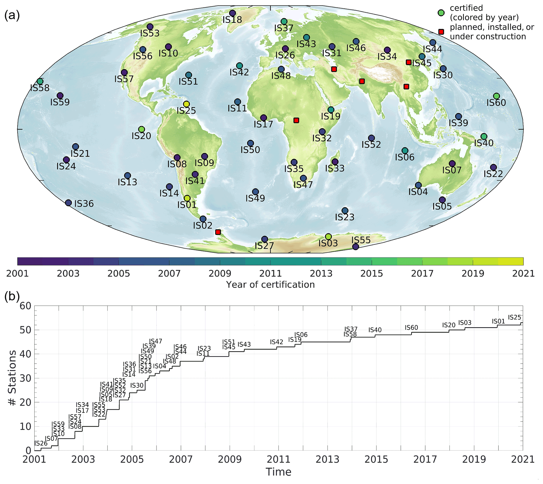
Figure 1 (a) Map of the IMS infrasound network with certified and planned stations (as of January 2021). This study covers the period from 2003 to 2020, during which the number of stations in operation was subsequently increased, as depicted by the approximate certification timeline (b). All certified stations are considered in this study, although the detection lists and products of IS25 (yellow circle) are not too expressive because of the short period during which the array was certified (end of 2020). The location of 1 of the 60 stations has not been determined yet. The map is based on the ETOPO1 Global Relief Model (NOAA National Geophysical Data Center, 2009; see also Amante and Eakins, 2009).

The temporal loss of sensor data diminishes a station's detection capability, which can also reduce the detection capability of the entire network, especially if a station consisting of only four or five sensors is affected. Extreme events such as wildfires, flooding, or lightning strikes are potential causes of data losses. Moreover, the station-specific environment creates a spatiotemporal variation in the detection capability, including incoherent wind noise and unwanted coherent infrasonic signals (e.g., Ceranna et al., 2019). While wind noise raises the detection threshold for coherent signals, unwanted but coherent signals may interfere the detection or discrimination of signals of interest. Therefore, the performance of the IMS stations is a key concern for the CTBT. Matoza et al. (2013) conducted a first comprehensive and systematic broadband analysis of historical IMS infrasound data and derived both station-specific coherent noise levels and overall performance characteristics. Ceranna et al. (2019) extended their broadband analysis by 4 years, thus covering the period from 1 April 2005 to 1 January 2015.

For this study, we reprocessed all historical IMS infrasound data from 1 January 2003 to 31 December 2020 using an advanced processing configuration.

2.2 Data processing

For automatically processing continuous waveform data of all infrasound stations, the Progressive Multi-Channel Correlation (PMCC) method (Cansi, 1995; Le Pichon and Cansi, 2003) is utilized. This array-processing algorithm proved to be efficient for detecting coherent low-amplitude acoustic waves within incoherent noise, as PMCC is routinely used for processing the IMS infrasound data at the IDC (Mialle et al., 2019). PMCC analyses the waveform data in successive, overlapping time windows and predefined frequency bands. The broadband analyses of Matoza et al. (2013) and Ceranna et al. (2019) were based on a PMCC implementation with variable window lengths and 15 logarithmically spaced frequency bands (Fig. 2a). Brachet et al. (2010) pointed out that such implementations enable the reprocessing of the full frequency range (0.01–5 Hz) in a single computational run and, thus, outperform the initial implementation that relied on linearly spaced frequency bands. An enhanced discrimination between interfering signals is envisaged with one-third octave frequency bands (Garcés, 2013). We pursue such an enhancement and apply the one-third octave frequency bands that are depicted in Fig. 2b, with second-order Chebyshev filters. The 26 bands cover the frequency range from 0.01 to around 4 Hz. The window lengths decrease with frequency from 600 to about 23 s. The time step is 10 % of the respective window length (90 % overlap).

The wavefront parameters of coherent plane waves are derived from cross-correlation functions and the arrival time delays between the sensor triplets of an array (Cansi, 1995); therefore at least three sensors need to be available. We use a consistency threshold of 0.1 s, which is in the range recommended by Runco Jr. et al. (2014). If more sensors are progressively incorporated (generally from the inside to the outside of an array), then the precision of the estimated parameters is refined while initial false detections (e.g., sub-scale correlated noise) can be discarded; overall, the localization accuracy increases with increasing array aperture (Cansi, 1995; Cansi and Le Pichon, 2008). Sub-networks (here triplets of array elements) can be predefined for the processing. It is of note that, beyond the minimum requirements for IMS infrasound arrays, not only the number of elements and the apertures but also the array geometries differ throughout the IMS (e.g., Marty, 2019), limiting the comparability of processing results between stations. For the same reasons, the sub-networks cannot be selected uniformly. However, as the frequency range of the processing reaches down to 0.01 Hz and, thus, longer periods and acoustic wavelengths, the sub-network geometries are generally chosen to exploit the maximum array element separations at each array (Matoza et al., 2013). Apart from that, the mixing of L-type and H-type sensors within a sub-network – the letter indicates the applied WNRS aperture – is avoided. Meanwhile, stations formerly equipped with mixed sensor types have been subsequently updated and homogenized. Apart from three exceptions where five sub-networks have proved to be efficient, we generally select four sub-networks for each array and thus follow the previous processing configuration by Ceranna et al. (2019). PMCC is supposed to reconfigure the sub-networks automatically in the case of a sensor failure (i.e., lack of data). Table A1 in the Appendix contains two columns with the array apertures and the chosen sub-networks, respectively.

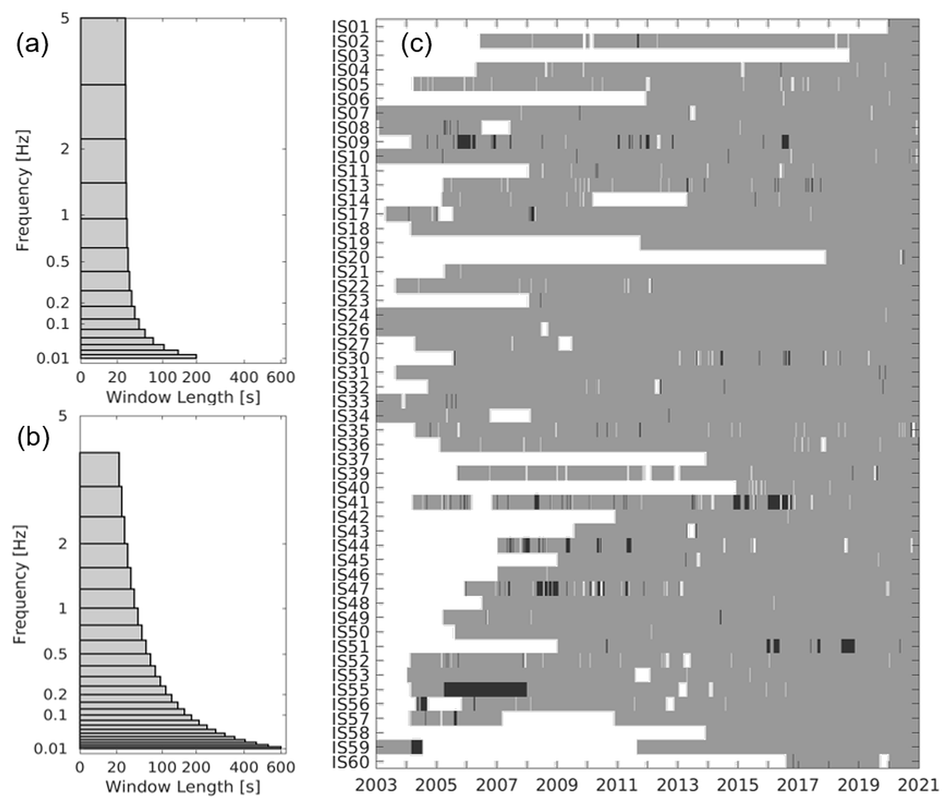
Figure 2 Comparison of the reprocessing configurations used to run the PMCC algorithm. (a) Log-spaced frequency bands as previously used by Ceranna et al. (2019). (b) One-third octave frequency bands applied in this study. The data availability (c) of the reprocessing results (gray) is depicted on a daily basis. Black lines indicate that raw waveform data were available but could not be processed, most often because the number of sensors was too low (<3). IS25 is not depicted because less than 1 month of data were available in the considered period (certified in December 2020). Note that panel (c) refers to the database available at the German NDC. As the data have subsequently been obtained from the IDC, the data coverage agrees with the data available through the vDEC; some exceptions might apply, as data gaps could be backfilled at the IDC, where available.

PMCC records a detected arrival within a frequency band and time window as a pixel. The estimated arrival parameters comprise, for instance, the back azimuth denoting the direction of origin, the frequency, the root mean square (RMS) amplitude, or the apparent velocity. The latter reflects the velocity of the wavefront in the x−y domain and is generally larger than the actual phase velocity because of the wavefront's inclination. Pixels adjacent to others in terms of frequency, time, back azimuth, and apparent velocity are grouped into detection families if at least 10 pixels contribute, i.e., PMCC assumes the same event to be the origin. Here, the chosen tolerance for the frequency criterion is a generous maximum of five bands, which is required due to the narrow bands at low frequencies. The maximum tolerances for the other parameters – 120 s, 10 to 5^∘, and 10 % to 5 % of the apparent velocity, respectively – are generally more constraining. The two latter parameters vary with the frequency bands, accounting for a potentially lower resolution of the parameters at very low frequencies, which is a result of the array response. The lower resolution may also apply to the amplitude parameters at very low frequencies because the data were not corrected for the array response, which is considered flat between 0.02 and 4 Hz (±3 dB). Hereinafter, a detection family is referred to as a detection. In the detection list for each station, a detection's wavefront parameters are averaged over all contributing pixels. PMCC neglects arrivals that are not associated with the dominant detection in a time–frequency domain (Cansi, 1995).

To our knowledge, standard thresholds for grouping pixels have not been specified, and threshold choices are a tradeoff between the probability of detection and the false alarm rate (e.g., Runco Jr. et al., 2014). The chosen minimum of 10 can be justified by significance in order to consider as many arrivals as possible (e.g., Che et al., 2019). Concerning an upper threshold, we constrain the family sizes to 200 pixels during the processing. This can split detections originating from a specific event, with a few exceptions when PMCC merges two families (i.e., >200 pixels). A higher threshold could summarize an event in only one family, which could be useful for certain applications. On the other hand, a higher threshold could result in mixing different sources (e.g., microbaroms) or in creating families with a long duration. Both could be at the expense of a parameter's detail when, for instance, the azimuth smoothly changes over time, either due to a moving source or due to propagation effects. The chosen upper limit of the number of pixels is therefore a compromise, in addition to the tolerances given above. Another potential source of splitting effects is the length of the data sequences processed at once. However, since we apply the processing to daily data files extended by ±5 min, an impact on the analysis is deemed marginal here. Nevertheless, detections of similar wavefront parameters that might have been split by PMCC could be merged to events during a dedicated post-processing.

We realized the reprocessing of all data for the period 2003 to 2020 using PMCC version 5.7.4 (CEA, 2018). This version has turned out to perform faster, and it apparently operates more reliably than previous versions, making it even more efficient. With the chosen configuration, processing the daily infrasound data of one station takes between 3 and 6 min on average (operating system is CentOS 6.10, with 32 GB RAM, 8 CPUs, and 3.4 GHz). The processing time varies with array size and the number of signal detections.

We post-process the detection lists to discard the most obvious artifacts. These include spurious signals lining up at the center frequencies of the processing bands (i.e., the mean frequency equals the center frequency) or at certain back azimuths. The majority of these signals are single-frequency-band detections (i.e., the minimum and maximum frequencies of a detection equal those of one particular frequency band). Seemingly, PMCC is sometimes unable to resolve the wavefront parameters correctly, resulting in a ringing artifact. The latter is also known from previous reprocessing configurations, and the concerned detections feature low family sizes. Here, we sort out detections exactly equaling any center frequency of the processing bands and detections of which the minimum and maximum frequencies differ by less than 6 mHz; this second criterion regards detections only covering the two lowest frequency bands. In the same context and after considering 2D histograms of mean frequency and family size, we additionally clean the detection lists by discarding detections with family sizes <40; for frequencies of <0.06 Hz, detections with <50 pixels are discarded. The applied criteria are a tradeoff between removing as many artifacts or false alarms and keeping as many actual events as possible. Effectively raising the lower family size threshold from 10 to 40 and 50 ensures the global comparability of the stations' detection lists and any derived product in terms of this parameter, even though the ringing artifact did not affect all stations to the same extent. Notwithstanding the above, the apparent velocities must range between 300 and 500 m s⁻¹ to be accepted as an infrasonic signature (e.g., Lonzaga, 2015). The availability of raw waveform data and processing results per station are shown, on a daily basis, in Fig. 2c.

3 Broadband detection lists

For the 53 IMS stations certified before the end of 2020 (see Fig. 1), the detection lists comprise a total of 81 267 602 entries over 18 years. In Fig. 3, the frequency distributions of all detections relative to the back azimuth (Fig. 3a) and the apparent velocity (Fig. 3b) as well as a 1D histogram (Fig. 3c) are shown.

3.1 Processing results

As stated by Le Pichon et al. (2010) and Ceranna et al. (2019), the detections can be roughly classified into three groups.

• (i.)

  Almost 40 % of all detections are signals with frequencies above 0.5 Hz. Many of these are of a transient nature with frequencies beyond 0.8 Hz. The sources include, for instance, volcanoes, surf, supersonic aircraft, explosions, and industrial activity. Their origin can generally be found within a few hundreds of kilometers from the station location since the transmission loss at these frequencies limits the propagation range. According to Sutherland and Bass (2004), the molecular attenuation coefficient for a 2 Hz wave is 2 orders of magnitude larger than for a 0.1 Hz wave. Therefore, the high-frequency azimuthal distribution is strongly linked to the station locations, as can be recognized by various peaks in Fig. 3a. At stations on islands or in coastal environments, surf is often the dominant source in the high-frequency infrasound range up to 20 Hz. Garcés et al. (2006) reported that surf energy can be found down to frequencies of 0.4 Hz, thus overlapping with the microbarom range. The main energy associated with surf, however, has generally been found between 1 and 5 Hz, as was demonstrated for IMS stations IS59 in Hawaii (Garcés et al., 2003), IS57 in California (Arrowsmith and Hedlin, 2005), and IS24 in Tahiti (Le Pichon et al., 2004). The 2D histogram shown in Fig. 3b indicates that the majority of high-frequency detections are tropospheric or stratospheric arrivals because they maximize at apparent velocities between 330 and 365 m s⁻¹. Following Lonzaga (2015), apparent velocities higher than ∼380 m s⁻¹ correspond to reflection altitudes in the thermosphere (>90 km), where the attenuation coefficient increases with altitude (Sutherland and Bass, 2004). Below 0.8 Hz, quasi-continuous sources, especially the growing impact of microbarom signals, lead to a smoother azimuthal distribution.

• (ii.)

  Almost 55 % of all detections have frequencies between 0.1 and 0.5 Hz. The maximum of the frequency distribution (Fig. 3c) reflects the dominant frequency of microbaroms at between 0.2 and 0.3 Hz. Explosions, meteorites, and volcanic eruptions are among the sources (Ceranna et al., 2019), but the microbaroms are the dominant signal type as every IMS infrasound station detects them in the course of the year (e.g., Landès et al., 2012; De Carlo et al., 2021). In Fig. 3a, both a pattern of easterly directions and a more dominant pattern of westerly directions with increased detection numbers reflect the characteristic annual cycle of microbarom detections, controlled by the stratospheric winds. An example of how the direction of the detected signals correlates with the middle atmosphere wind conditions is presented in Fig. 4, showing the processing results of IS27 in Antarctica. IS27 is located near the Antarctic Circumpolar Current (ACC), which is a major source of microbaroms in the Southern Hemisphere throughout the entire year, whereas high-frequency sources are rare in this region. The predominant arrival directions of microbaroms change from northwest in the austral winter to northeast in the summer.

• (iii.)

  The minority (<6 %) of the detections are characterized by frequencies lower than 0.1 Hz. At these frequencies, infrasonic waves can travel long distances through the atmosphere. The corresponding phenomena, however, are either very rare – e.g., large meteorites like the Chelyabinsk fireball (Pilger et al., 2015) – or spatially confined to middle to high latitudes – e.g., MAWs or auroras. MAWs are the most frequent source of these phenomena and are associated with strong tropospheric winds over mountainous regions (e.g., Hupe et al., 2021); hence, the station location relative to the sources becomes relevant again. Moreover, the transmission loss is reduced at these frequencies, limiting the importance of the stratospheric waveguide. Northerly and southerly directions (Fig. 3a) and higher apparent velocities (Fig. 3b) dominate the detections. It is of note that aurora infrasound is often characterized by apparent velocities above 500 m s⁻¹ (Wilson et al., 2010) and will therefore hardly be represented in the detection lists. Also, high apparent velocities can partly be caused by a reduced array response at low frequencies due to the geometry of the station, resulting in a poorer estimation of this parameter.

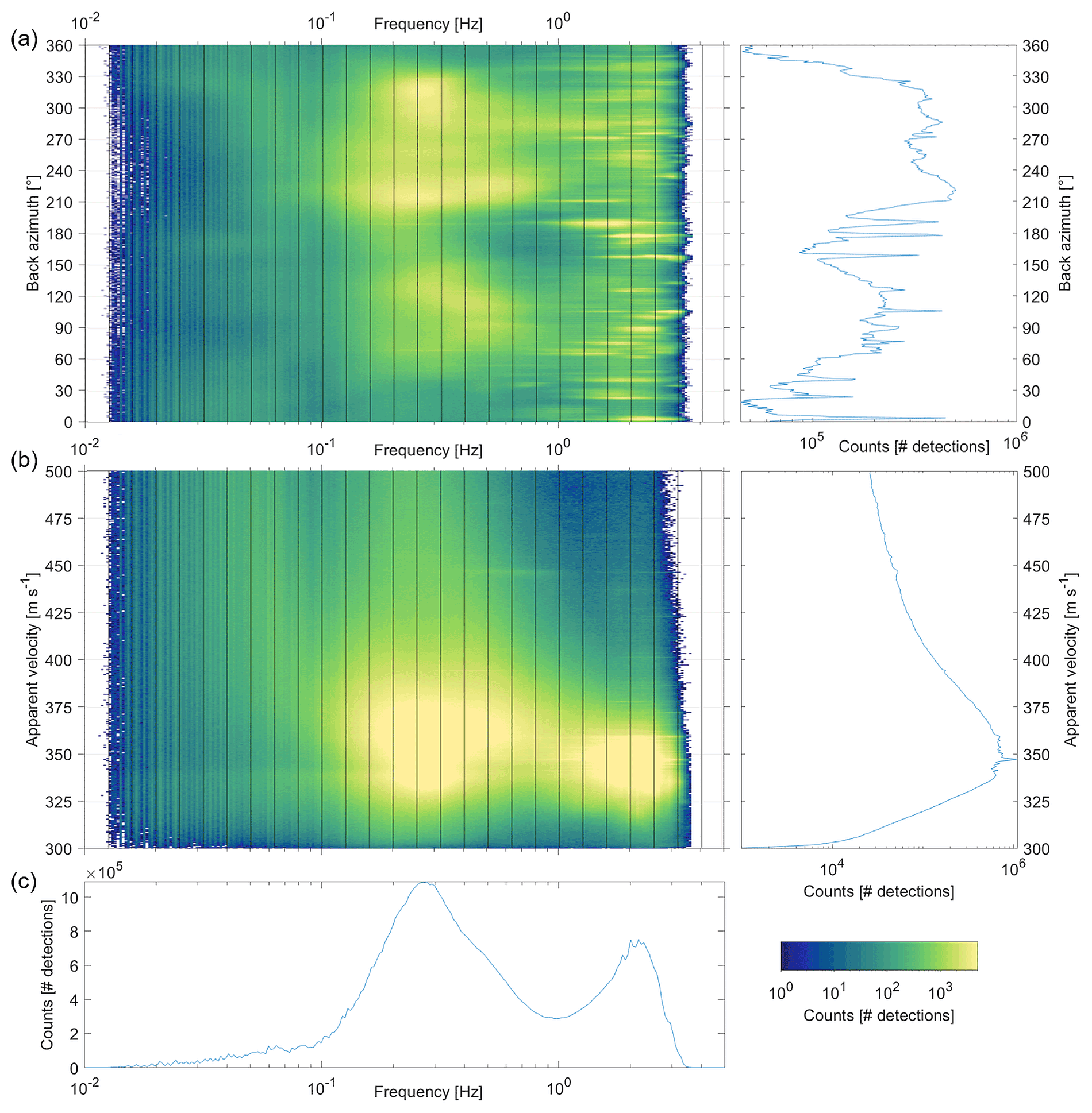
Figure 3 (a) Frequency–azimuth and (b) frequency–velocity distributions (left panels) of all detections at 53 stations from 2003 to 2020. The sub-panels of (a) and (b) on the right show the 1D histograms for azimuth and velocity, and panel (c) shows the frequency. In the 2D histograms, the solid black lines depict the frequency bands of the processing with widths of the one-third octave (see Fig. 2b). The number of detections refer to bins of approximately $\mathrm{1}/\mathrm{10}$ of the frequency bandwidths and 0.5^∘ (a) or 0.5 m s⁻¹ (b), respectively.

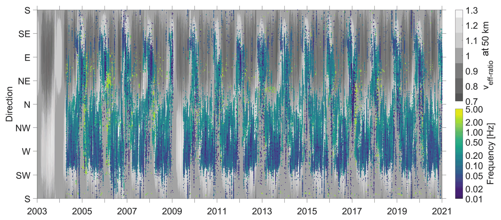
Figure 4 Detections at IS27 from 2004 to 2020, with color-coded frequency. The lack of detections in 2009 is because of the array's relocation and revalidation (see Sect. 2.1). The v_eff-ratio at around 50 km altitude (grayscale) was calculated from temperature and wind profiles obtained from ECMWF's HRES operational atmospheric model analysis as the maximum ratio between 40 and 60 km. Dark gray background colors (v_eff-ratio<0.95) indicate unfavorable propagation from the respective direction, whereas favorable conditions in light gray (v_eff-ratio≥0.95) often coincide with an increased number of detections. The majority of detections are microbaroms (0.1–0.5 Hz) originating from the Antarctic Circumpolar Current (northwesterly to northeasterly directions).

3.2 Comparison with the previously used PMCC configuration

We compare the frequency–azimuth histograms of the detection lists of the different configurations using the example of IS26 in Germany. In Fig. 5a, all detections with family sizes >20 resulting from the 15-band configuration by Ceranna et al. (2019) are processed for 12 years (2003–2014). It is noteworthy that the 15-band configuration was limited to family sizes of 100 instead of 200 (both with exceptions) and, hence, the lower threshold of 20. Ringing artifacts at the respective frequency band centers were discarded at the expense of some true detections (white lines). Although the latter might also happen when using the newer version and configuration, the cleaning from artifacts seems more successfully applicable to the respective center frequencies, as the white lines of Fig. 5a almost disappear in Fig. 5b. Hence, based on the criteria explained in Sect. 2.2, discriminating between true detections and artifacts succeeds better with the 26-band configuration. With this updated processing scheme, we obtain around 82 % more detections (in total 1.879×10⁶) within the same time. Due to the narrower frequency bands, the average difference between the minimum and maximum frequency within a family has decreased from 1.09 to 0.82 Hz. This will have contributed to the increased number of detections. On the contrary, the average family size has increased from 72 to 169 pixels and the average duration from 90 to 105 s, suggesting that the chosen one-third octave band configuration provides detections with a larger signal content. These enhanced features better highlight particular sources in the frequency–azimuth histograms, for instance a cluster at 0.3 to 0.6 Hz and 15 to 20^∘ that can hardly be recognized in Fig. 5a. More detections enable an enhanced discrimination between sources, and as the processing artifacts can be subtracted more easily using the newer configuration, low-frequency sources are better represented. At IS26, two clusters around 0.07 Hz and southerly directions become more evident. The centroids of these clusters seem to be shifted to slightly higher frequencies than before (by around 0.02 Hz). We do not observe such shifts for detection clusters at frequencies >0.1 Hz. However, compared to the low-noise models of selected IMS infrasound stations presented by Marty et al. (2021), the spectral (microbarom) peaks of Figs. 3 and 5 appear to be shifted to slightly higher frequencies by ∼0.05 Hz. We cannot rule out some frequency uncertainty in the PMCC detections resulting from leakage effects due to the configuration settings. Garcés (2013) discussed potential energy leakage when assessing the benefit of using one-third octave bands for infrasound data processing. Hanning windows, which are implemented in PMCC for tapering the time windows and which were also applied by Marty et al. (2021), should generally reduce potential energy leakage (e.g., Brachet et al., 2010). The shift in the frequency range <0.1 Hz could also result from better-constrained detection parameters using the one-third octave processing scheme.

In the high-frequency range, the newly implemented processing configuration neglects sources beyond 4 Hz (previously 5 Hz). This upper-band threshold has been adapted to reduce the amount of local clutter and rather focus on signals that have long-range propagation. Moreover, the accuracy (correlation) of the detections decreases with increasing frequency because of the corresponding wavelengths relative to the array apertures and the selected sub-networks (Sect. 2.2). A few sources might be lost due to this adaption, compared to the 15-band configuration, including small volcanic eruptions. Nevertheless, a maximum of around 4 Hz is sufficient for capturing a global picture of the coherent ambient infrasonic noise and relevant events in the context of CTBT monitoring and verification. Overall, the example of IS26 shows that the newly implemented processing configuration with PMCC version 5.7.4 outperforms the formerly used one with PMCC 4.4.

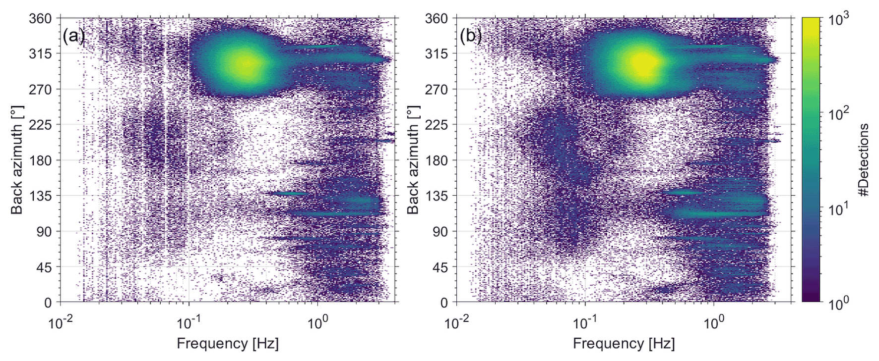
Figure 5 The 2D histograms of broadband detection lists for IS26, Germany, based on (a) 15 logarithmically spaced bands (Matoza et al., 2013; Ceranna et al., 2019) and (b) 26 one-third octave bands for the PMCC configuration. The bin sizes equal those of Fig. 3 ($\mathrm{1}/\mathrm{10}$ of the one-third octave frequency bands and 0.5^∘). The detections of panel (a) were processed using PMCC version 4.4 and cover the years 2003–2014. Panel (b) is built upon the more recent PMCC version 5.7.4, and the temporal coverage is adapted to that of panel (a) for comparability. The white vertical lines near the center frequencies in panel (a) result from cleaning the detection list of ringing artifacts. With the newer version and configuration, the cleaning is easier to narrow down to the respective center frequencies.

3.3 Data quality parameter

As stated in Sect. 2, missing sensors or other array issues can affect the processing performance and thus the detection parameters. The number of available sensors, N_avail, and the number of sensors contributing to a PMCC detection, N_contr, are crucial indicators for the quality of a detection. When comparing long-term time series, changes in the array size, N_max, also have to be taken into account. For the quality of a detection, two PMCC output parameters are considered. The correlation coefficient, r_c, denotes the correlation of an arrival between the contributing sensors; here, r_c is taken as the mean over all arrivals within a family. The Fisher ratio, F, puts the variance of noise plus the coherent signal in relation to the variance of noise; hence, F exceeds 1 only if a coherent signal is recorded (Melton and Bailey, 1957). The Fisher correlation analysis in the time domain (e.g., Fisher, 1992) can be an alternative method to PMCC for detecting coherent signals within uncorrelated noise, but PMCC computes F for each detection as an additional output parameter.

We combine all of these parameters empirically to define a single parameter as a proxy for the relative quality, Q, as follows:

$$\begin{array}{}\text{(1)}& Q={\displaystyle \frac{\mathrm{1}}{\mathrm{2}}}\left(r_{\mathrm{c}}\cdot w_{r_{\mathrm{c}}}\left(f\right)+{\displaystyle \frac{N_{\mathrm{contr}}}{N_{\max }}}\right)\cdot {\displaystyle \frac{F}{N_{\mathrm{avail}}-\mathrm{1}}},\end{array}$$

which is the arithmetic mean of the two summands in the parentheses times the Fisher ratio relative to the available sensor number. For this calculation, we weight the correlation coefficient with a frequency-dependent function, $w_{r_{\mathrm{c}}}\left(f\right)$. This function compensates for the fact that low-frequency detections have a larger correlation coefficient due to the narrower frequency bands than high-frequency detections (Fig. 6).

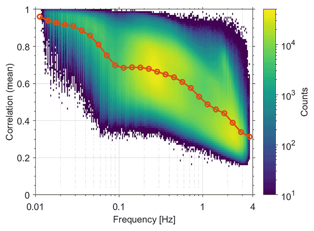
Figure 6 Correlation coefficients of all detections (2003–2020; all stations) vs. frequency. The red line depicts the mean correlation for each of the 26 frequency bands. Bin sizes are $\mathrm{1}/\mathrm{10}$ of a frequency band and 0.01, respectively. The frequency-band-dependent weighting function $w_{r_{\mathrm{c}}}$ in Eq. (1) weights the correlation coefficients of all detections, such that the mean correlation of each frequency band would equal 0.5.

Q ranges between 0 and 1, as the correlation and the relative sensor availability (i.e., the first two summands of the parentheses in Eq. 1) do. In the case of a large F, the last factor of Eq. (1) can exceed 1; if this results in Q>1, then we define Q=1. The consideration of Q enables the assessment of the quality of the detections; i.e., the lower Q is, the lower potentially at least one of the weighted correlation coefficients, the relative sensor coverage, and the Fisher ratio is. We do not implement a threshold for Q, as the cause for a reduction in any of these parameters can be manifold (e.g., GPS clock failure, flooded sensor, and background noise level). Moreover, an anomaly can affect only specific detection parameters while others remain unaffected and may still be of use. Figure 7 shows such an example for IS05 in Australia. Here, it is noteworthy that the Fisher ratio also correlates with the frequency, similar to the correlation coefficient. Nevertheless, we do not apply a weighting like for the correlation coefficient, as F seems appropriate to indicate anomalies in certain parameters. At IS05, the back azimuths (Fig. 7a) follow the annual cycle of the propagation conditions similar to Fig. 4, and these detections have generally been consistent since 2004. The amplitudes (Fig. 7b), however, exhibit anomalies until 2012, and in both 2018 and 2019, even more detections feature particularly large amplitudes (near 1 Pa) before returning to the normal range (10⁻³ to 10⁻¹ Pa). The anomalously large amplitudes correspond to relatively low values of Q (Q<0.12), which is here caused by very low Fisher ratios. Anomalies in the back azimuths or the frequencies are not recognized during that period. According to the IDC in Vienna, temporary issues with the WNRS for one of the sensors were reported in early 2019, which potentially caused the observed anomalies here.

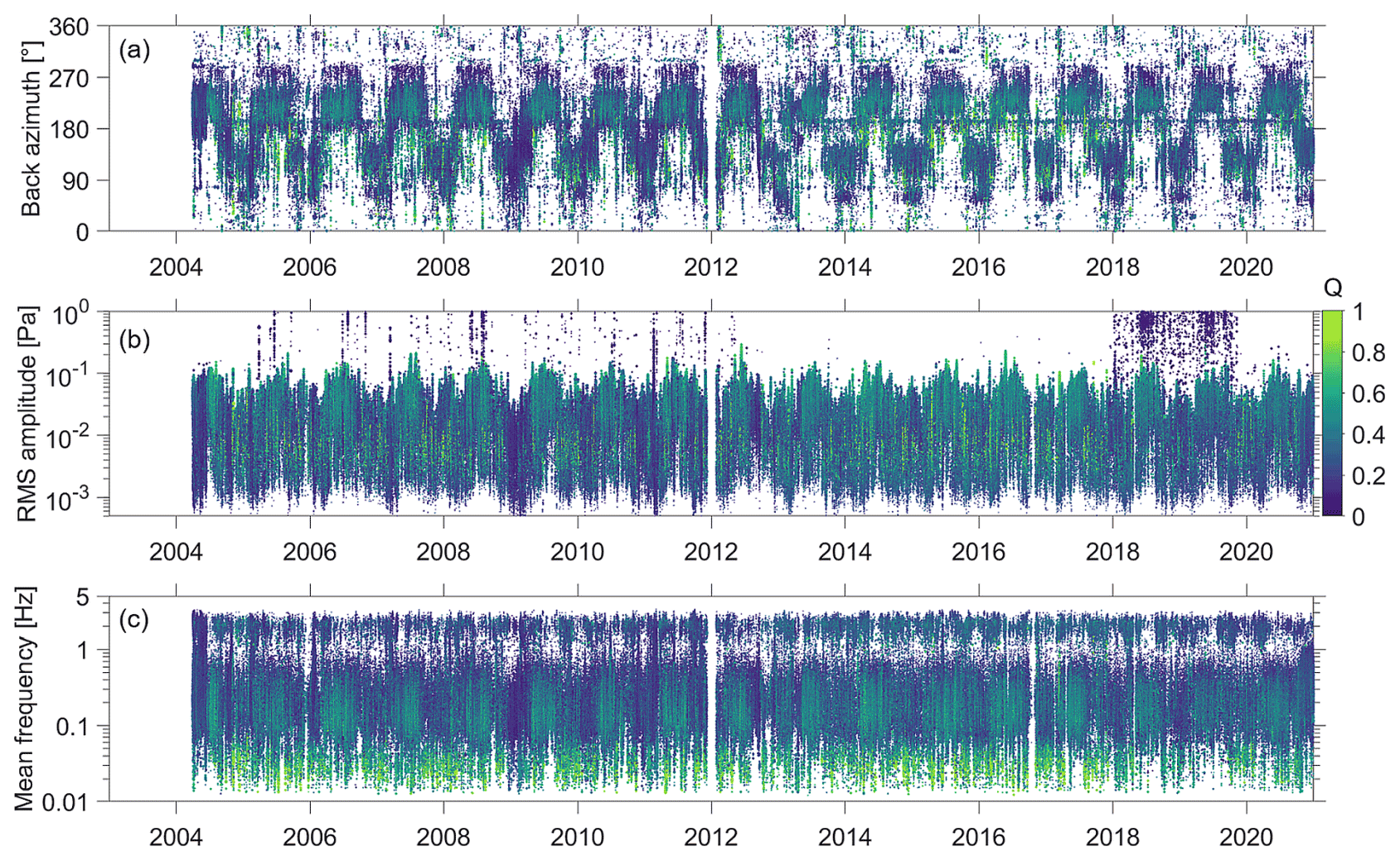
Figure 7 Time series of the detection parameters back azimuth (a), amplitude (b), and frequency (c) for IS05, Tasmania (Australia). The color bar applies to all panels and depicts the quality parameter Q, defined in Eq. (1). Figure C1 in the Appendix shows IS05 detections with Q>0.5 only.

In general, Q tends to be a bit higher at lower frequencies (Fig. 7c) because F is not weighted like r_c. Another feature in Fig. 7 is low values of Q in late 2008 and early 2009, while lacking obvious anomalies in any of the shown parameters. The congruent drop to Q<0.4 can be traced back to lower F again, accompanied by the fact that fewer sensors – temporarily only four out of eight – contributed to the PMCC detections. Overall, this parameter allows for identifying both naturally caused anomalies and station performance issues. Therefore, it is a valuable addition to the detection parameters of the data products and is potentially of interest to station operators and NDCs, for instance, if they do not have the resources to compute such a data set.

4 Data products

From the comprehensive detection lists, we define four data products that cover different time–frequency domains. Here the time reflects the temporal resolution of the data set, as we provide detection parameters at distinct, equally spaced time steps. The time step interval matches the window length; hence, there is no overlap. Note that we define the data products based on the mean frequencies of the detections. The minimum and maximum frequencies of the detections (families) are not a criterion and can thus cover the entire frequency range of the processing. The defined products are tailored to specific phenomena and spectral peaks in the mean frequency distribution (Fig. 3c). We decided to split the microbarom frequency range into two products because the peak frequency of the spectrum would generally dominate the detections within a single product. A second product potentially allows for better discrimination of the sources in this frequency range. In total, the four products cover almost 75 % of all detections.

A low-frequency product (Hupe et al., 2021a) incorporates detections with mean frequencies of between 0.02 and 0.07 Hz, which encompasses only 3.5 % of all detections. The time step and window length are 30 min. Since MAWs are likely the mostly detected source in this frequency range (e.g., Hupe et al., 2021), we name this product “maw”.

The second product covers the spectral peak near 0.25 Hz in the frequency distribution of all station detections (Fig. 3c). The frequency range of this product is 0.15 to 0.35 Hz (36 % of all detections). Since the majority of the detections are (low-frequency) microbaroms, the product is named “mb_lf” (Hupe et al., 2021b). The temporal resolution is 15 min.

The third product ranges from 0.45 to 0.65 Hz (10.1 %), which includes the upper-frequency spectrum of microbaroms, and is therefore named “mb_hf” (Hupe et al., 2021c). The temporal resolution is 15 min.

The secondary spectral peak around 2 Hz (Fig. 3c) is covered by the high-frequency (hf) product (Hupe et al., 2021d), with mean frequencies between 1 and 3 Hz and a temporal resolution of 5 min. One-quarter (25.5 %) of all detections contribute to this product, where surf is likely the mostly detected source.

For the first product, all family sizes ≥50 are considered to ensure a consistent threshold over this product's frequency range after cleaning the detection lists from artifacts. For the other products, the threshold of 40 holds, which matches the threshold for cleaning the detection lists from artifacts at frequencies beyond 0.06 Hz (see Sect. 2.2).

4.1 Parameters

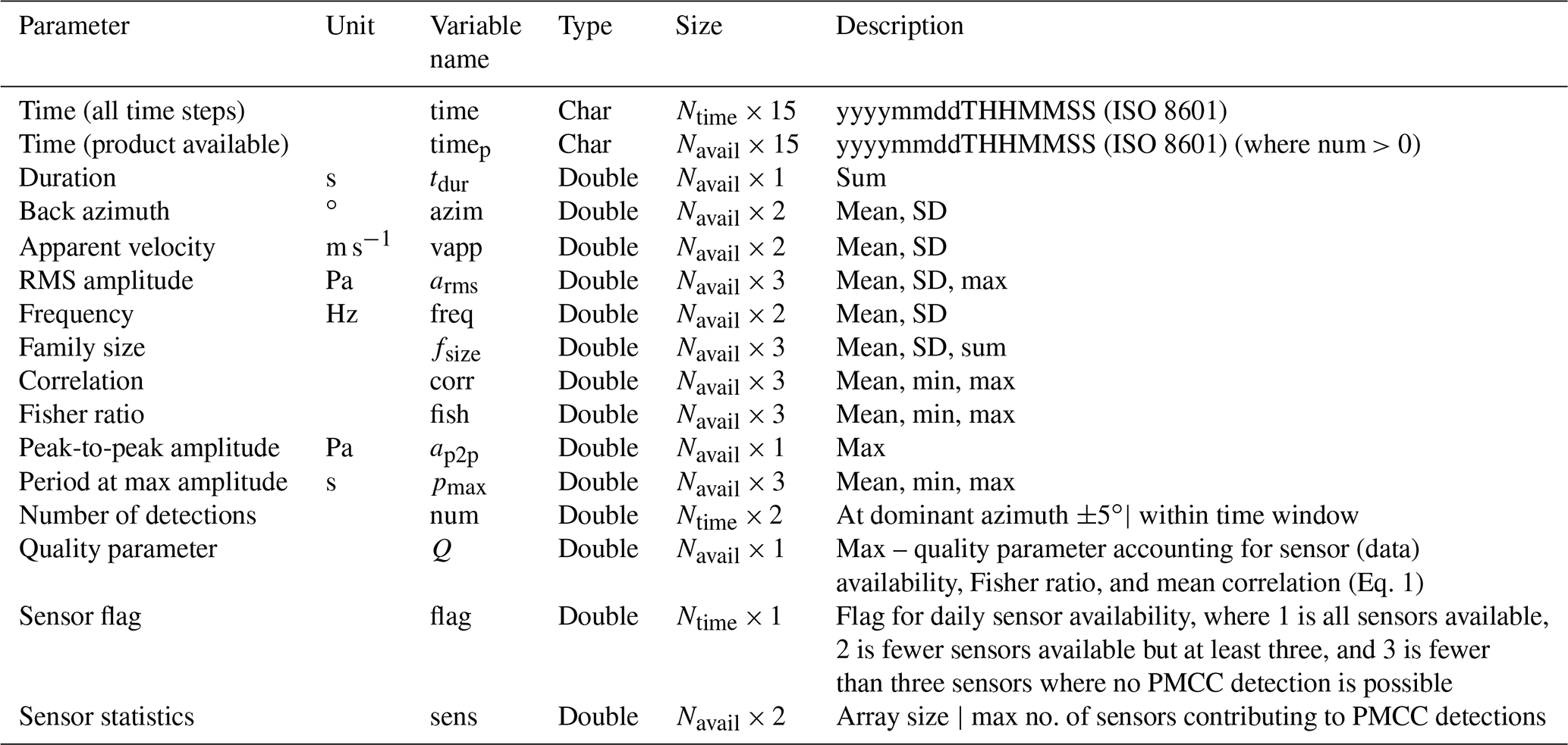
A parameter provided at a time step summarizes the parameters of dominant detections within the time window since the previous time step. To identify dominant detections, 1D back azimuth histograms are considered in which the family sizes of the detections are stacked per 1^∘. Stacking the family sizes by azimuth and over the time windows compensates a large portion of the potential split of detections caused by the processing configuration threshold of 200 (Sect. 2.2), except from the transition at the discrete time steps. The location of the maximum of the histogram defines the dominant direction (i.e., the most signal content arrived from that direction). If more than one maximum exists, then the direction with the highest Q scores off the others. All potential detections within ± 5^∘ tolerance from the dominant direction are then considered for calculating the mean back azimuth weighted by family size, which is consequently very close to the dominant direction. Based on the same detections and weighting, further selected detection parameters (see Table 1) are accordingly summarized and represent the dominant detections. The majority of the parameters contain information about the weighted standard deviation of all detections within the time window respective to the calculated (dominant) mean. This standard deviation (detection based) is detached from the one provided by PMCC (pixel based), which is not considered here. For some parameters, deviating or additional quantities are provided, as detailed below.

Table 1 Overview of the data product parameters provided in the netCDF files for each station. All mean, min, max, and sum values correspond to all detections within the dominant azimuth $\pm \mathrm{5}{}^{\circ }$. The mean values are weighted by family size of the detections. The standard deviation (SD) accounts for all detections within the considered time window and refers to the calculated mean. N_time denotes the total number of time steps, whereas N_avail denotes the number of time steps with product parameters available.

4.1.1 Time parameters

All products contain a time vector of length N_time, which is the number of equally spaced time steps from 1 January 2003 to 1 January 2021. Another time vector (time_p) is of length N_avail; it defines the time steps for which the product parameters are defined. The evaluated parameters refer to the time window since the last nominal time step (i.e., for the maw product with a resolution of 30 min, for instance, the time stamp of 1 January 2021 00:00 UTC summarizes all detections since 31 December 2020 23:30 UTC).

For the duration, neither the mean nor the standard deviation is calculated; instead, the durations of all detections with the dominant azimuth tolerance range are summed up during the time window. Implying that these detections originate from the same source, the total duration of the dominant signals is more conducive for the source characterization than the mean duration. Moreover, this method partly compensates a potential bias if detections were split by the configured family size threshold.

4.1.2 Wavefront parameters

Following the definition of the back azimuth being dominant in terms of family size, the tolerance range, and the weighting described in Sect. 4.1, the back azimuth parameter represents the dominant direction of a signal within the time window. The standard deviation is calculated with regard to the determined mean. What both quantities have in common is that they are weighted by the family size of the detections to account for the signal content and thus the significance of the single detection. As distinct to the mean, the standard deviation is calculated over all detections within the time window to illustrate the variability in the detections. Consequently, the standard deviation in back azimuth can exceed the tolerance range of $\pm \mathrm{5}{}^{\circ }$.

The mean and the standard deviation are also provided for the frequency, the apparent velocity, the RMS amplitude, and the family size. Here, the weighted mean values are again based on those detections that match the dominant azimuth $\pm \mathrm{5}{}^{\circ }$, whereas the standard deviation with regard to the respective mean accounts for all detections within the time window weighted by family size. The family size variable additionally contains the sum, analogous to the duration, as this conveys an impression of how strong or long-lasting the potential source was.

The RMS amplitude variable additionally contains the maximum amplitude of the dominant direction. The peak-to-peak amplitude variable is exclusively provided as the maximum value within the dominant direction $\pm \mathrm{5}{}^{\circ }$, as this will be of interest for yield estimations of (chemical) explosions. For instance, the Los Alamos National Laboratory (LANL) yield relation requires the wind-corrected amplitude and distance as input (e.g., Whitaker et al., 2003), and the maximum amplitude of the related detections likely results in a more realistic estimation than the mean.

The period at the maximum amplitude also serves as an input parameter to energy and yield estimations. For instance, two relations of the Air Force Technical Application Center (AFTAC; ReVelle, 1997) are commonly used to estimate the energy of fireballs entering and burning up in the atmosphere (e.g., Ott et al., 2019; Pilger et al., 2020). The product variable of this parameter contains the mean, the minimum, and the maximum of the dominant detections, enabling both lower and upper yield estimates and thus accounting for uncertainties.

4.1.3 Quality parameters and missing values

For the correlation and the Fisher ratio, the mean, minimum, and maximum are also provided. For the newly introduced Q, it is the maximum only. The additional variables of “flag” and “num” are the only parameters that are defined at each time step, even if the product is not defined, for instance, due to unavailable raw data or the lack of processing results. The variable flag provides an indication of whether the data of all sensors were available (flag =1). If at least three but not all sensors were available, then it is flag =2. If fewer than the required three sensors were available, then flag has the value 3. Then the variable num is zero. Otherwise, num indicates the number of detections per time window (first column of num) and with the dominant azimuth $\pm \mathrm{5}{}^{\circ }$ (second column), which are contributing to the standard deviations and means, respectively. The first column of the “sens” variable denotes the nominal array size (number of sensors), which remains constant or increases, but is not supposed to decrease, i.e., station revalidation periods are not accounted for. The second column is a number between 3 and the array size (N_max) denoting the maximum number of sensors contributing to the dominant PMCC detections. Overall, these variables enable an assessment of the quality of the data products or allow the comprehension of missing values.

4.1.4 Station parameters

Each product file contains the longitude, latitude, and elevation of the respective station as the variables “long” (“lon.” in netCDF), “lat”, and “elev”. The coordinates (WGS84) are rounded to the second decimal and allow users who are not familiar with the IMS network to apply the parameters, e.g., for triangulation, or to collect atmospheric model profiles of temperature and wind for the sites and along the propagation path between the infrasound station and the anticipated or determined source location.

4.2 Format

All parameters are stored in netCDF files with the extension .nc, including metadata about the parameter variables (Table 1). One file per infrasound station, year, and product is released. The file sizes depend on the number of time steps for which a product is available. They do not exceed 4 MB (maw product), 8.5 MB (mb products), or 25 MB (hf product), respectively. The file names include the IMS infrasound station, the year, the abbreviated designation of the data product and its frequency range and the temporal resolution representing the time step and window length (e.g., IS26_2013_mb_lf_0.15–0.35Hz_15min.nc). For details on how to retrieve the data products, please see Sect. 6.

4.3 Temporal coverage

The maximum number of time steps per data product (N_time in Table 1) results from the considered period (2003 to 2020) and the temporal resolution of the data products. Table B1 in the Appendix lists the portion of time steps at which a product is available per station ($N_{\mathrm{avail}}/N_{\mathrm{time}}$). Overall, and at the majority of the stations, the mb_lf product is the one covered the best, with 23.5 % on average. Due to the operational time of a station (see Figs. 1b and 2c), its detection capability, or its location relative to sources, this portion varies between 1.1 % (IS51, Bermuda) and 52.2 % (IS04, Western Australia). Such variability also applies to the other products, of which the overall coverage is lower than 10 %.

5 Case sensitivity and potential applications of the data products

To show the capability of the data products, we choose both global and event-based approaches. We focus on two major explosive events that were of special interest for demonstrating the detection capability of the IMS infrasound network and recent volcanic eruptions which are a significant natural hazard to civil security around the globe. For the coherent ambient noise, a global view of the data products is provided.

5.1 Warehouse explosion in the port of Beirut, Lebanon, on 4 August 2020

One recent event of interest is the devastating explosion in the port of Beirut on 4 August 2020, as the explosive yield was estimated in the order of the IMS network's design goal, using different waveform and remote sensing technologies (Pilger et al., 2021a). Infrasound detections were reported at five IMS arrays at distances of between 2450 and 6250 km from the source. The first signals arrived at IS48 in Tunisia and IS26 in Germany between 17:06 and 17:30 UTC. It is of note that the dominant frequencies differed at these stations, which is reflected in the mean values of 2.57 and 0.70 Hz, respectively. The frequency ranges of the multiple arrivals theoretically cover the mb and hf products, but the mean frequencies of the associated detection families do not. As the products are based on the latter, IS26 detections of the Beirut explosion are represented in the two mb products (17:15 and 17:30 UTC), whereas IS48 detections can be found in the mb_hf (17:30 UTC) and hf (17:10, 17:15, 17:20, 17:25, and 17:30 UTC) products (Fig. 8a). The maximum peak-to-peak amplitudes provided in the products correspond approximately those values found by Pilger et al. (2021a), hence enabling reasonable yield estimates using the LANL yield relation (Whitaker et al., 2003) when additionally incorporating the atmospheric wind conditions.

5.2 Fireball near Chelyabinsk, Russia, on 15 February 2013

Before the recent volcano eruption of Hunga, Tonga (e.g., Matoza et al., 2022; Vergoz et al., 2022), the large meteorite and its fragmentation at around 30 km altitude, which according to Brown et al. (2013) released an explosive energy equivalent of roughly 500 kt TNT equivalent, produced the strongest signal that has been recorded by the IMS infrasound network, with 20 out of 42 operational stations detecting it (Le Pichon et al., 2013). At the closest station (540 km), IS31 in Kazakhstan, signatures of the large fireball arrived around 30 min after the impact at 03:20 UTC and covered a broad frequency range. As illustrated in Fig. 8b, the event is represented in four data products of IS31 (maw, mb_lf, mb_hf, and hf). The first signatures from 25^∘ slightly deviated in back azimuth from the theoretical one (23.7^∘ from IS31 to 54.85^∘ N, 61.45^∘ E, i.e., south of Chelyabinsk; see Pilger et al., 2015). The back azimuth deviation increased with time, which allows the inferring of the trajectory of the fireball (e.g., Pilger et al., 2020). Combining the information of the different data products would also enable the assessment of the temporal variation in azimuth in this case, encouraging the investigation of the propagation and source characteristics. Notably, the maw product (04:30 UTC) of Fig. 8b does not align with the first low-frequency PMCC detections before 04:00 UTC. However, these are broadband detection families whose mean frequencies are higher and therefore not assigned to the maw product. Within the 30 min after 04:00 UTC, a few low-frequency detections result in the maw product signature of 04:30 UTC.

Apart from the IS31 detections, at other detecting stations, long-period infrasonic waves were the dominant ones excited by the fragmentation and traveled very long distances. At IS53 in Alaska, for instance, the signals were still recorded after circling the globe twice (Le Pichon et al., 2013). At stations more distant than IS31, such as IS43 in Russia (1510 km) or IS26 in Germany (3280 km), the explosion-like event was detected with frequencies below 0.1 Hz. The maw product includes these signatures, e.g., for IS26 at 07:30 UTC from 54.8^∘ (standard deviation 1.7^∘), with the total duration of five detections being 585 s and Q=0.94. For IS43, two entries in the maw product at 05:30 and 06:00 UTC sum up to a duration of 41 min (2461 s) distributed over 19 detections. The minimum and maximum values for the period at the maximum amplitude are of the order of those reported by Le Pichon et al. (2013). For IS26, for instance, our product gives 18.6 and 30 s (Le Pichon et al., 2013, report 20 and 35 s), respectively, and the mean is 24.8 s. Translated into yield estimates using the AFTAC relation (ReVelle, 1997), a TNT-equivalent range of between 90 and 640 kt results, while the mean corresponds to 290 kt. This range gives an impression of the uncertainty of the empirical yield relations, both at one station and when considering a set of stations. Le Pichon et al. (2013) eventually used the mean values of 14 stations to specify the yield of the fireball at roughly 460 kt TNT.

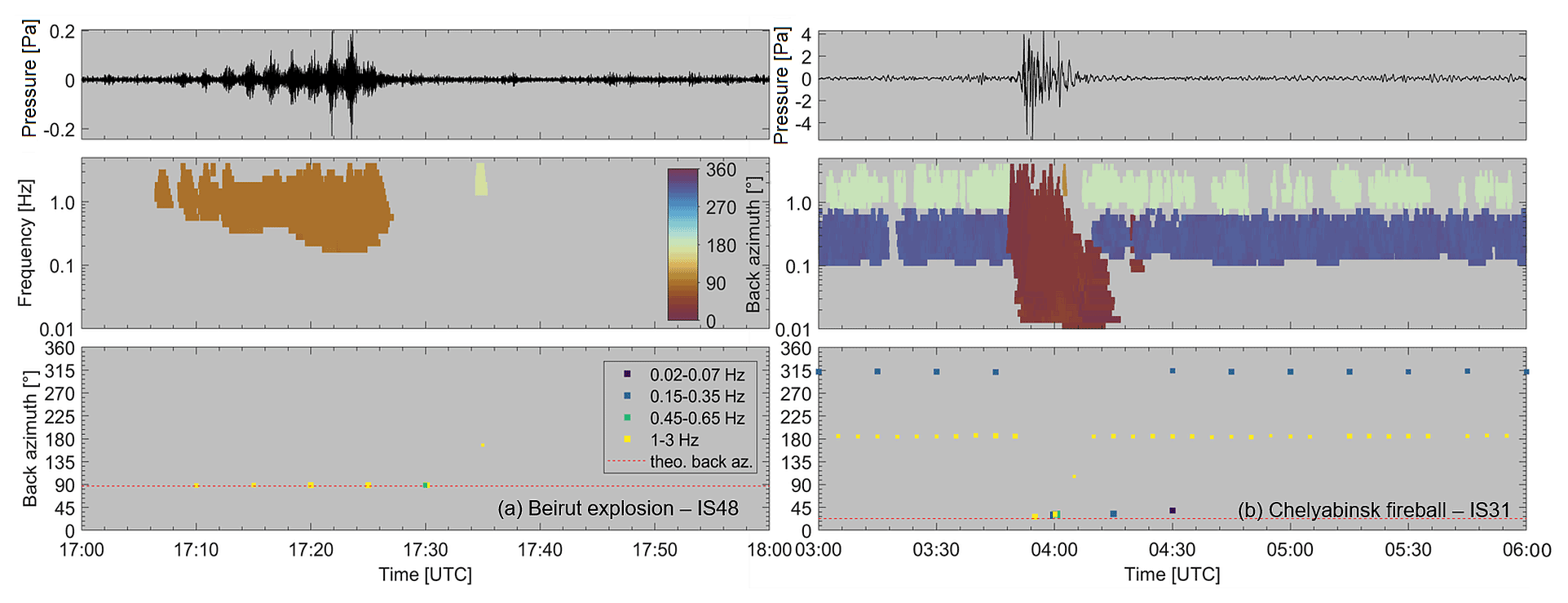
Figure 8 Waveform beam (top), PMCC result (center), and data products for (a) the Beirut explosion detected at IS48, Tunisia (2450 km distance), on 4 August 2020 and (b) the Chelyabinsk fireball detected at IS31, Kazakhstan (540 km), on 15 February 2013. The waveform beams correspond to the theoretical back azimuths and third-order Chebyshev bandpass filters (0.5–4 and 0.02–2 Hz, respectively). The legends of panel (a) apply to panel (b) too. The relative marker size of the products (bottom panels) depicts Q. The dashed red lines depict the theoretical back azimuths from an array to the source. It is of note that the mb_lf and hf signatures caused by the fireball interrupt the series of IS31 detections from a northwesterly direction ($\sim \mathrm{315}{}^{\circ }$), most likely microbaroms, and from a southerly direction.

Overall, infrasound recordings can be helpful to detect, locate, and characterize large meteorites entering uninhabited regions where they remain unnoticed by the public, such as the Bering Sea fireball on 18 December 2018 (Tillman, 2019), which was the second-strongest fireball ever detected by the IMS infrasound network (e.g., Pilger et al., 2020). Infrasound observations can serve as a primary source of information or complement observations by other technologies (e.g., Ott et al., 2019).

5.3 Volcanic eruptions

One of the recent volcanic eruptions was Taal in the Philippines, beginning on 12 January 2020 and lasting for 10 d (Global Volcanism Program, 2013). It was assigned a Volcanic Explosivity Index (VEI) of 4 and is in this respect comparable with the Eyjafjallajökull eruption on Iceland in 2010, which heavily affected global air traffic due to its ash plume. The explosive eruption phases of the Eyjafjallajökull volcano in April and May were recorded by four infrasound arrays of the IMS (IS18, IS26, IS43, and IS48) at distances between 2200 and 3700 km, plus 10 regional infrasound arrays in Europe within 2200 km of the source (Matoza et al., 2011b). As an example, we note that especially the mb_hf and hf products of IS26 in Germany contain a series of corresponding detections between 18 April and 2 May 2010.

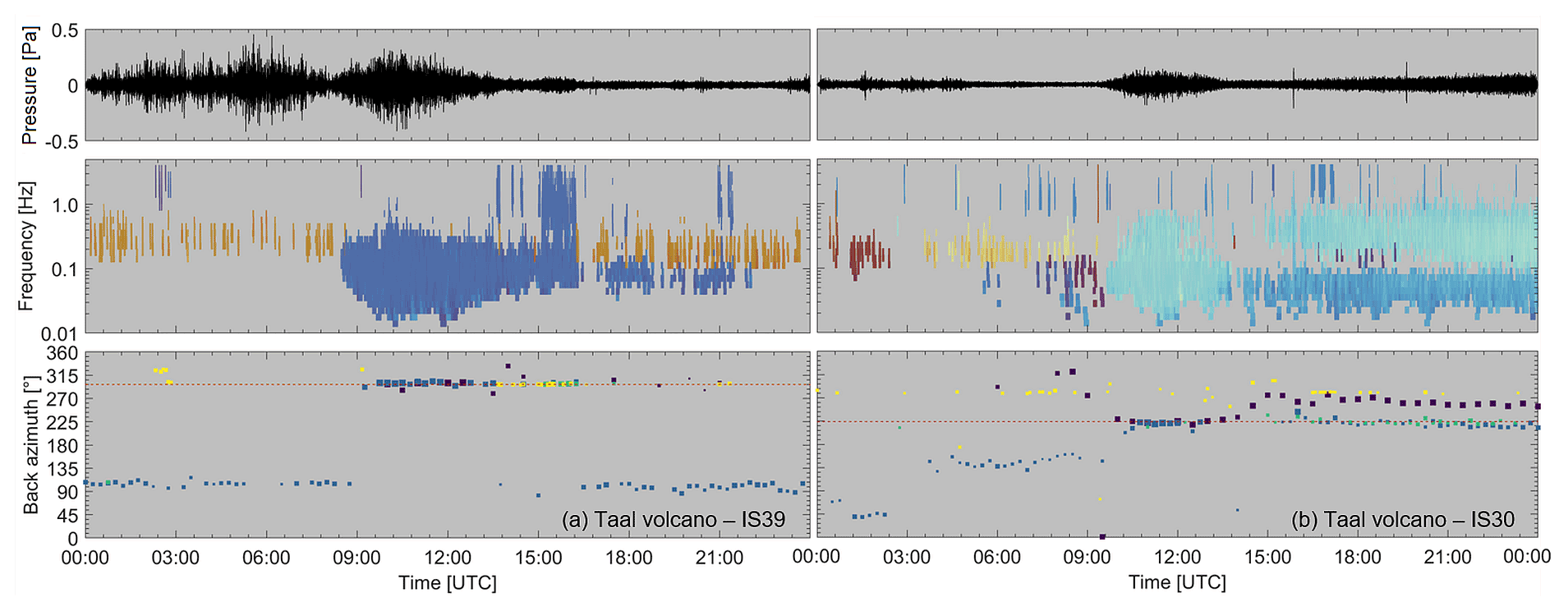
Figure 9 Waveform beam (top), PMCC result (center), and data products of (a) IS39, Palau (1640 km distance), and (b) IS30, Japan (3050 km), on 12 January 2020, when a strong eruption of the Taal Volcano (the Philippines) occurred. The waveform beams correspond to the theoretical back azimuths and a third-order Chebyshev bandpass filter (0.05–4 Hz). The dashed red lines depict the theoretical back azimuths relative to the Taal Volcano. At IS39, the broadband signatures cover all data products. The colors and symbols of Fig. 8 apply.

For the Taal Volcano eruption in 2020, Perttu et al. (2020) found infrasonic signatures at IS39, Palau, which they used to estimate the plume height to 17 km maximum. Such information is essential for running ash dispersion models and thus forecasting the ash plume in the atmosphere, allowing both air traffic control and the Volcanic Ash Advisory Center (VAAC) and local authorities to implement timely safety measures (e.g., Matoza et al., 2019, and references therein). Figure 9a shows the back azimuths of the IS39 data products on 12 January 2020. The back azimuths of arrivals beginning around 09:00 UTC are consistent with the direction of Taal (297^∘). The onset is distinguished in the mb_lf product because the initial direction of dominant detections suddenly changes by about 180^∘, followed by hf detections until 16:30 UTC. In addition to IS39, we have found consistent detections at IS30 in Japan. The IS30 data products (Fig. 9b) reproduce the detections well, particularly the maw and mb_lf products. After 15:00 UTC, the mb products of IS30 show features within $\mathrm{224}\pm \mathrm{15}{}^{\circ }$ that possibly indicate ongoing activity beyond the end of that day.

Several other active volcanoes are covered by our data products, including the explosive eruptions of Calbuco, Chile (see Matoza et al., 2018), Stromboli, Italy (Le Pichon et al., 2021), and Raikoke, Kuril Islands (McKee et al., 2021), to name a few examples that were recently reported. Besides singular events, the IMS also captures quasi-continuous eruptive activity, among which are the serial explosions of two volcanoes – Lopevi and Yasur – in Vanuatu (e.g., Le Pichon et al., 2005). These are represented in the hf products of IS22 in New Caledonia. Figure 10 shows the back azimuths of the IS22 products in 2020, with hf signatures from 45^∘ almost throughout the whole year being associated with the Yasur volcano at around 400 km distance. Slight deviations from the theoretical directions are caused by crosswinds; therefore, these signatures remain useful for probing the atmospheric propagation conditions (Le Pichon et al., 2005) that occur over a long period and are subsequently approaching climatological timescales.

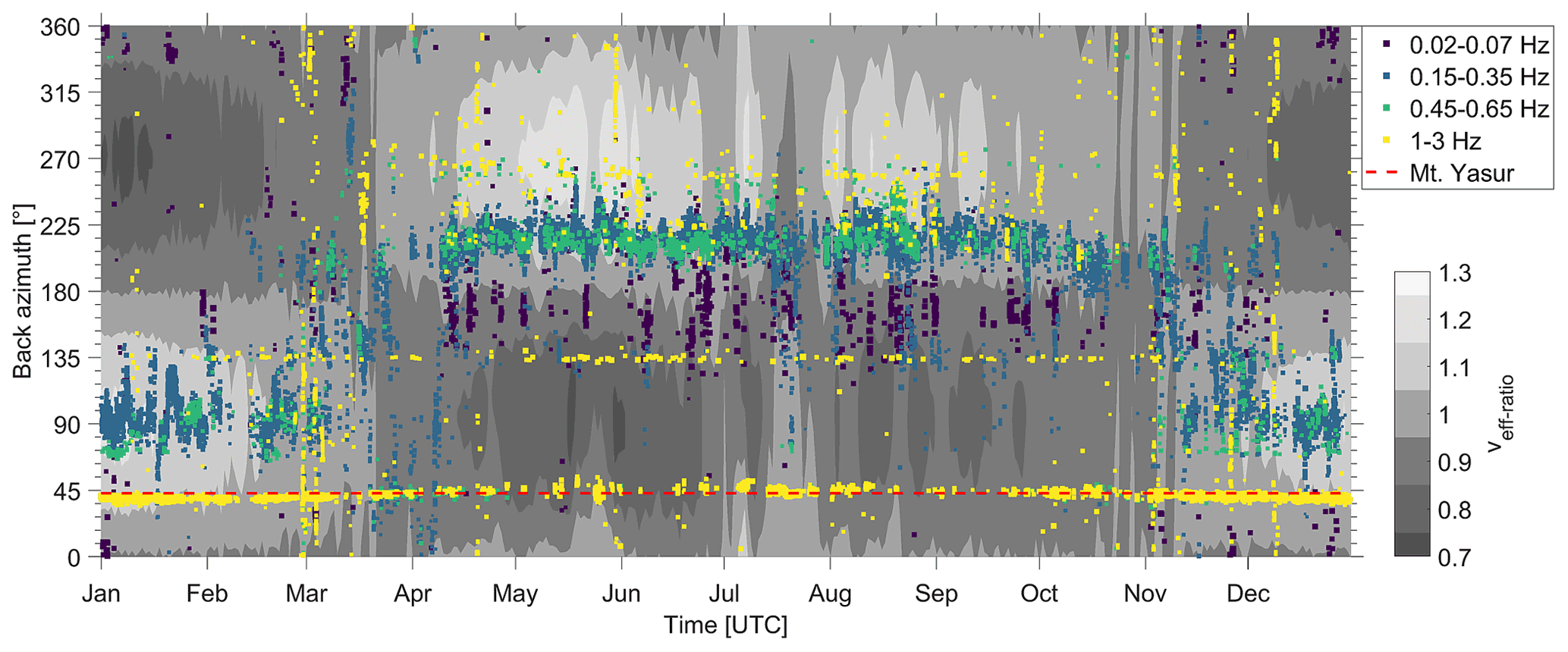
Figure 10 Back azimuth of IS22 data products (color-coded) in 2020, with the v_eff-ratio (grayscale; analogous to Fig. 4) shown in the background. If the v_eff-ratio is around or larger than 1, then arrivals from the corresponding direction are favorable in terms of the local propagation conditions.

Overall, we intend that our open-access data products of up to 18 years for 53 IMS infrasound stations can be utilized systematically to monitor and characterize active volcanism around the globe, following the example set by Matoza et al. (2017), who also incorporated the Eyjafjallajökull's explosive eruptions. Moreover, the data products can serve as an input to and reference data set for recent advancements in early warning applications. For instance, the calculation of a volcano infrasound parameter (IP) at regional and local arrays around Mount Etna (Ripepe et al., 2018) has successfully been applied to more distant IMS arrays by Marchetti et al. (2019), demonstrating that the IP enables warnings prior to explosive eruptions that can be useful to VAACs. As the IP is a product of the mean infrasonic amplitude and the number of detections in a certain time window, our data products provide the relevant information for its calculation. Since these products are not available in real time at this stage, a next step will be to demonstrate the capability of integrating the data products into early warning applications based on past eruptions. This will pioneer the early release of tailored data products in the future.

5.4 Coherent ambient noise and atmospheric dynamics

The detections of microbaroms are related to the annual cycle of the middle atmosphere winds controlling the effective sound speed and, thus, the directivity of the ground-to-stratosphere waveguide (e.g., Landès et al., 2012). De Carlo et al. (2021) recently applied the comprehensive detection lists described in Sect. 3 for validating an updated microbarom source and propagation model that was developed by De Carlo et al. (2020). Our objective is that the data products defined in Sect. 4 can also serve as a reference database for future model developments. The temporal resolution of the mb data products (15 min) is higher than that of commonly used atmospheric models (1 h or more) or the ocean wave model on which the De Carlo et al. (2020) model relies (3 h).

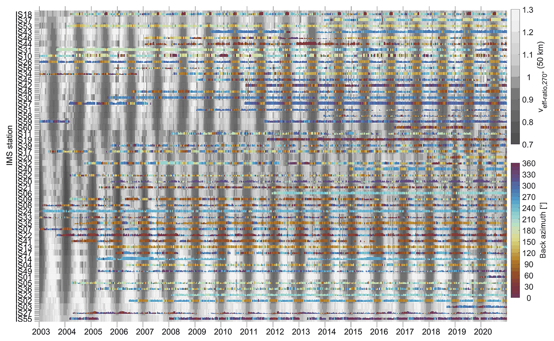
To demonstrate the products' capability, we reproduce the global microbarom activity using the mb_lf product of the 52 stations with at least 1 year of data availability – thus excluding IS25 – in Fig. 11. The roughly weekly variability of the mean dominant back azimuths (color-coded) is superimposed on the v_eff-ratio that illustrates the stratospheric waveguide conditions for zonal propagation (back azimuth 270^∘), with light gray colors depicting favorable conditions for eastward propagation. It can be assumed that dark gray background colors represent favorable westward propagation conditions. The global overview highlights the annual reversal of the stratospheric winds as the direction of detections generally follows this pattern. It resembles the global picture given by Ceranna et al. (2019), who provided such an illustration for the entire frequency range covered by the processing. This underlines that microbarom detections constitute by far the most detected phenomenon within the IMS infrasound network, even if other events, such as those described in the previous subsections, are not subtracted from the mb_lf product here. For a comparison, we provide Fig. C2, which qualitatively hardly differs from Fig. 11 at first glance and relies on the comprehensive detection lists of Sect. 3, covering a broader microbarom frequency range (0.1–0.5 Hz). The chosen time step (4 d) and window length (8 d) are identical.

In the Southern Hemisphere, the dominant arrival direction switches between the southwest (austral winter) and southeast (austral summer), as the ACC produces major microbarom sources throughout the year (e.g., De Carlo et al., 2021). Therefore, the detectability mainly depends on the stratospheric waveguide direction. In the Northern Hemisphere, a clear pattern only establishes during the winter, while arrival directions relate to the northern parts of the Atlantic and Pacific oceans, corresponding to southwesterly back azimuths at high-latitude arrays and northwesterly back azimuths at almost all other stations. In the summer, the westward stratospheric jet is weaker than the eastward jet during the winter, and the distribution of the continental landmasses additionally prevents a clear pattern.

When showing the global view based on the mb_hf product (Fig. C3), the overall picture is similar, but some station-specific differences can be recognized. Most strikingly, IS30 in Japan exhibits a seasonal pattern in the mb_hf product that is not recognizable in the other figures, which can be explained by its location relative to the microbarom sources. The Pacific Ocean to easterly directions is obviously dominant for the long-period microbaroms throughout the year, as it is nearly contiguous with the station. At shorter periods, smaller and marginal seas can be a relevant source of microbaroms where low-frequency microbaroms lack. At IS30, the Sea of Japan, or the East China Sea, are potential candidates for the arrivals from westerly directions in the winter. Such an effect likely causes differences at other stations too. Therefore, the two separate mb data products enable the user to discriminate between such sources, which may be useful for microbarom model validations or, for instance, studies focusing on marginal seas. Moreover, these mb products can be of use for assessing atmospheric models, as microbarom detections can reveal uncertainties in the representation of the middle atmospheric temperature and winds (e.g., Hupe et al., 2019) and temporary changes in the middle atmosphere conditions, such as during SSW events (e.g., Assink et al., 2014). If detected variations in the mb products cannot be associated with the atmospheric circulation pattern and its variability, then they could also be another indication for station performance issues, along with the quality parameter (Sect. 3.3).

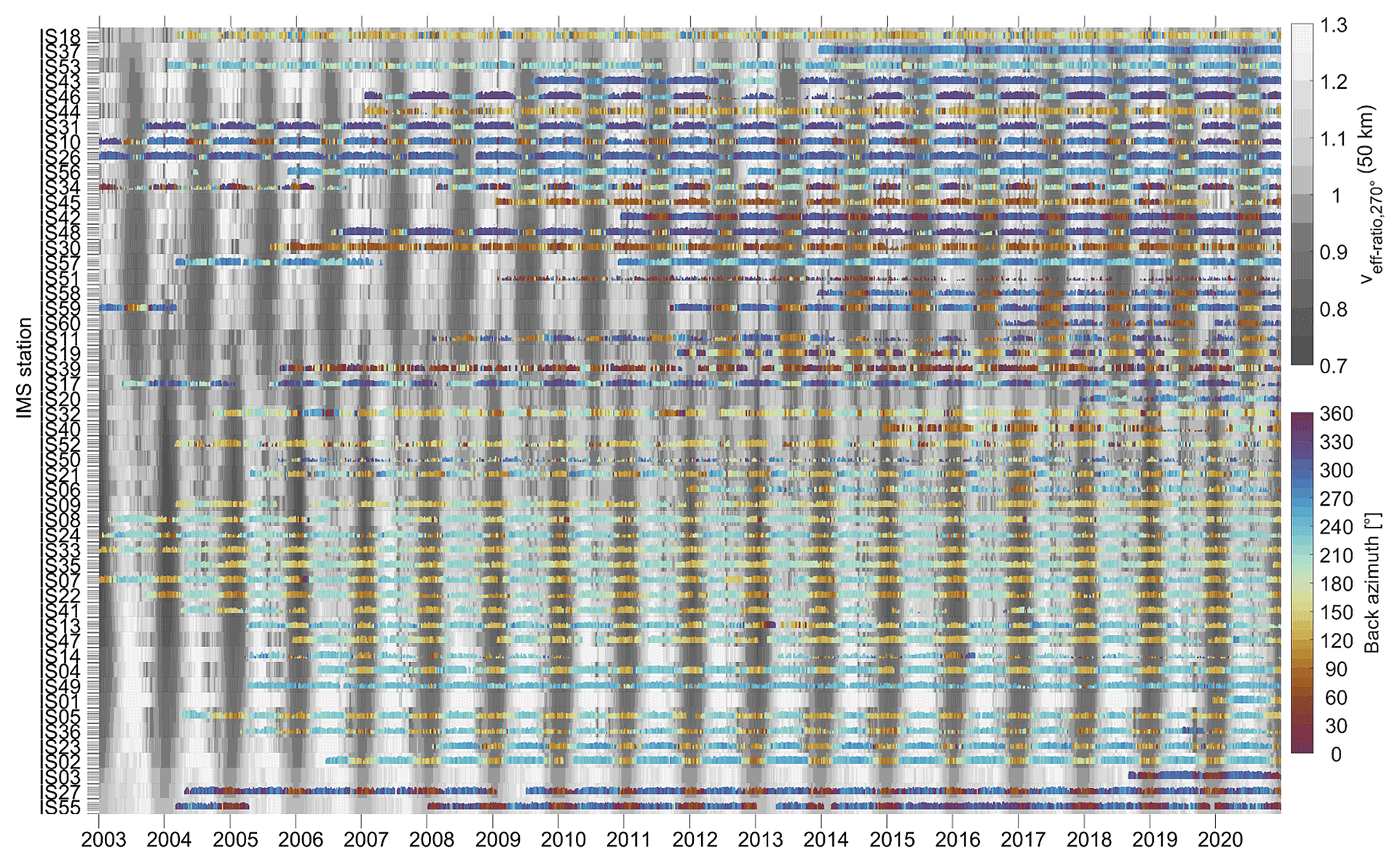
Figure 11 Global picture of the back azimuth variation in the mb_lf product (0.15–0.35 Hz), averaged in time windows of 8 d. For each time step (4 d), the mean back azimuth is color-coded. Grayscale depicts the v_eff-ratio calculated from the ECMWF temperature and wind profiles at each station analogously to Fig. 4 but for arrivals from westerly directions (270^∘). IS20 marks the transition from the Northern to the Southern hemispheres.

Analogously to Fig. 11, we illustrate the hf product in Fig. 12. At the majority of the stations, the hf product is also related to the annual cycle of the stratospheric wind directions, depicted by the v_eff-ratio, such that the dominant directions often change with the wind reversals during the equinoxes. However, the dominant directions significantly differ from those of the mb products. As stated in Sect. 3, signals in the higher-frequency range more likely originate from regional and local sources because the propagation range is more constrained than for very low-frequency acoustic waves. The difference is particularly striking at stations located in the Southern Hemisphere, where many IMS arrays are installed on islands or close to the coastlines, and therefore, surf is a major source. For instance, the dominant back azimuth at IS24, Tahiti, is associated with westerly to southwesterly directions and hardly changes with the stratospheric wind reversal, which agrees with the observations by Le Pichon et al. (2004). Other island stations such as IS06, IS13, IS14, and IS23 also exhibit a relatively consistent dominant direction over the year, which is indicative of sources in the near field. In the Northern Hemisphere, this applies to the coastal stations IS19, in Djibouti, and IS59, in Hawaii. The latter station is consistent with the northwesterly directions observed by Garcés et al. (2003), who found a correlation between the infrasonic amplitude and the wave height. Arrowsmith and Hedlin (2005) confirmed this correlation for IS57 in California. They noted a difference in that the observed signals propagated over a longer range of around 200 km, and they determined a seasonal cycle in the number of surf detections from northwesterly directions, with a maximum in the winter season. This agrees with the dominant directions shown in Fig. 12. In the summer season, signals from southeasterly directions prevail, corresponding to the stratospheric circulation. Besides surf, a frequently occurring source can be industrial noise. For instance, the dominant back azimuth (around 280^∘) at IS30 in Japan corresponds to (southern) Tokyo Bay, with the industrial areas of Yokohama and Kawasaki and several power stations in the near field.

Figure 12 Similar to Fig. 11 but for the hf product (1–3 Hz).

Finally, the maw product is shown in Fig. 13, also following the examples of the global microbarom detections. It qualitatively represents the global view provided by Hupe et al. (2021); here we can use a higher resolution since the updated processing results in a larger number of detections at low frequencies (Sect. 3). Hupe et al. (2021) already noted that a seasonal pattern can also be recognized for the MAW detections, but the location of the arrays relative to the global MAW source regions is more relevant and evident in the back azimuths. For a comparison, Fig. C4 reproduces Fig. 13 based on the comprehensive detection lists. The main difference is the number of detections, which results from the time window of the product summarizing the dominant detections. The maw product may be of use for revisiting the source localization and further investigating source excitation of MAWs, following the comprehensive study of MAW detections at IMS infrasound detections by Hupe (2018), which was based on PMCC version 4.4.

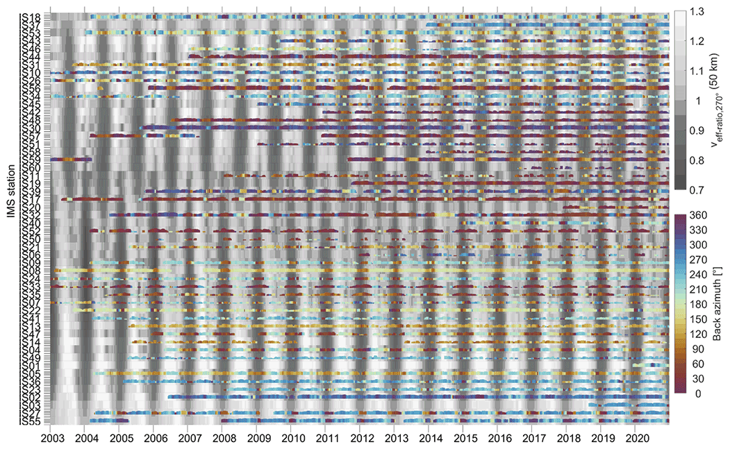
Figure 13 Global picture of the back azimuth variation in the maw product (0.02–0.07 Hz), averaged in time windows of 30 d. For each time step (7 d), the mean back azimuth is color-coded. Grayscale depicts the v_eff-ratio calculated from the temperature and wind profiles (ECMWF) at each station for arrivals from westerly directions (270^∘). IS20 marks the transition from the Northern to the Southern hemispheres. Note that the vertical extent of each colored line, which denotes the number of detections at a logarithmic scale, is not directly comparable to that of Fig. 11 (different scaling).

Table 2 DOIs and references related to the infrasound products. The file sizes refer to the 2003–2020 data sets and will increase when more years are added to the .zip files.

6 Data availability

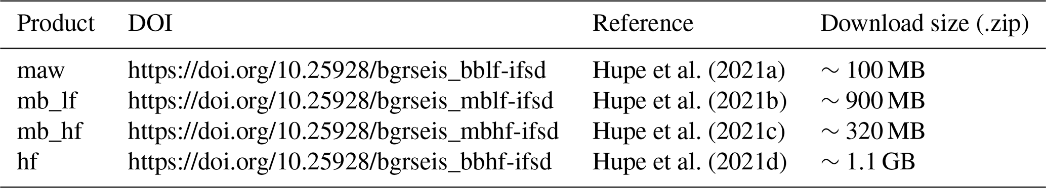
The infrasound data products are openly accessible through the product center (Geoportal; https://geoportal.bgr.de/, last access: on 26 July 2022) of the Federal Institute for Geosciences and Natural Resources (BGR), which is the German NDC (Pilger et al., 2017). For each of the four product types, the Geoportal contains one data set that is assigned a digital object identifier (DOI; Table 2). Each data set is provided as a compressed .zip file. The .zip files contain a README file, yearly subdirectories with the netCDF (.nc) data files for all certified stations, and a simple MATLAB code that reads and plots the netCDF data of a station.

With the DOI as the search item, a data product can be found in the Geoportal using the search function. Alternatively, search for “infrasound” and set the filter “dataset” to display a list of all available infrasound data products (i.e., not limited to these four data sets). The direct landing page of a DOI (e.g., https://doi.org/10.25928/bgrseis_bblf-ifsd for maw; Hupe et al., 2021a) opens the metadata page of the respective product (this page may take a few seconds to load). The download link of a data set (.zip file) is displayed on the right-hand side of both the search result and the metadata page (Download – Select type – Download-Link).

BGR's Geoportal ensures the long-term availability of the data products, while the Creative Commons Attribution 4.0 International license (CC BY 4.0, https://creativecommons.org/licenses/by/4.0/, last access: 22 July 2022) applies. Therefore, any reference related to the use of the data products should cite this accompanying paper and the respective DOI of the product type, stating the year and station (or summarize this information appropriately), e.g., for the hf products, Hupe et al. (2021d) https://doi.org/10.25928/bgrseis_bbhf-ifsd, and stations IS26 and IS27 for 2011–2020.

Access to the IMS network's data, including raw waveform recordings of the infrasound stations, can be granted upon request through the virtual Data Exploitation Center (vDEC) of the IDC at https://www.ctbto.org/specials/vdec (last access: 29 October 2021).

Information about the high-resolution (HRES) operational atmospheric model analysis of the European Centre for Medium-Range Weather Forecasts (ECMWF), produced by the Integrated Forecast System (IFS), can be found at https://www.ecmwf.int/en/forecasts/datasets (last access: 29 October 2021). The relevant data used to calculate the v_eff-ratio are available in ECMWF's Archive Catalogue (https://apps.ecmwf.int/archive-catalogue/, last access: 8 December 2021), which is published under the CC BY 4.0 license.

7 Conclusions

Gaining a global picture of the coherent infrasound wave field is essential for CTBT verification and is beneficial for probing the dynamics in the middle atmosphere where operational observation methods are sparse. The updated processing configuration with one-third octave frequency bands, and the extended time period of consideration (2003–2020), advance the global reference data set of infrasound detections. There are four derived data products that summarize the comprehensive, highly resolved detection lists that have been created to make infrasound data accessible for a broader community. The products of different temporal resolutions and frequency ranges cover numerous infrasound sources. They can serve as reference databases for various applications. These encompass model developments or validations within the infrasound and atmospheric community, infrasound data assimilation for atmospheric models, or early warning systems for civilian security.

The definition of the products signifies that only the dominant detections within a time window are represented by the open-access database. Moreover, methods other than the PMCC algorithm may be more appropriate to obtain a comprehensive picture of the azimuthal soundscape because PMCC itself focuses on the dominant signal within a time window and frequency band. For instance, CLEAN beamforming (e.g., Den Ouden et al., 2020) and the vespagram method (Vorobeva et al., 2021) have been demonstrated to be capable of capturing multiple sources at selected IMS stations. Nevertheless, PMCC is a well-established processing method in the infrasound community and is used by the IDC. The comprehensive detection lists described in this study have already been used for the validation of a microbarom model (De Carlo et al., 2021) and the identification of an extremely remote volcano (De Negri et al., 2022). The dominant infrasound signal summaries are also useful for civilian security applications. Examples of recent volcanic eruptions show that the different data products cover these and other transient events appropriately.

The openly accessible data products of detection lists do not replace the privileges of either vDEC account access to raw infrasound data or of nominated users who have access to the Reviewed Event Bulletin of the IDC. The tailored data products, in terms of frequency ranges and temporal resolution, instead simplify the utilization of infrasound data – for instance, by user groups who do not have the resources to compute such a data set or who are not experienced in the use of array-processing methods such as the PMCC algorithm. Additional parameters provided with the products enable all types of users to assess the relative quality of the data, which is also valuable for identifying potential temporary station performance issues. We therefore assume that this archived database, currently spanning 18 years, can contribute to advancing the use of infrasound observations for scientific applications and the development of prototypes for early warning systems. The introduced quality parameter will be further elaborated on, while, in parallel, work considering the station- and time-dependent confidence intervals on wave parameters is ongoing (Kristoffersen et al., 2022a). These so-called PMCC metrics are published separately (Kristoffersen et al., 2022b) to help identify anomalies in the data and its products. It is envisaged that the product databases are regularly updated, implying at least an offset of 3 months, which is in line with the current vDEC regulations that permit access to raw data after this embargo time. For early warning systems (e.g., volcanic eruptions) or atmospheric model assimilations, however, it would be necessary to provide automated data products in near-real time in the future.

Appendix A: IMS infrasound station information

Table A1 IMS infrasound array properties, certification year (see Fig. 1), and selected sub-networks for the PMCC processing. If elements were added to the array, then the year of this modification (revalidation) and the previous number of array elements are indicated in parentheses behind the latest number of elements. These changes did not alter the apertures because the new sensors were installed within the existing arrays. The sub-network information contains triplets of sensors numbers, referring to the latest channel numbering (e.g., L1, … L4, … or H1, … H8, …). If two types (H and L) are still defined (IS18 was homogenized to H in 2016, but the name was not changed), then the corresponding letter is indicated. The column code denotes the country (ISO 3166 code) as part of the five-digit station codes (e.g., I26DE instead of IS26). We omit the five-digit notation in our data products for simplicity, but it is common in IDC products and the vDEC.

Appendix B: Data product availability

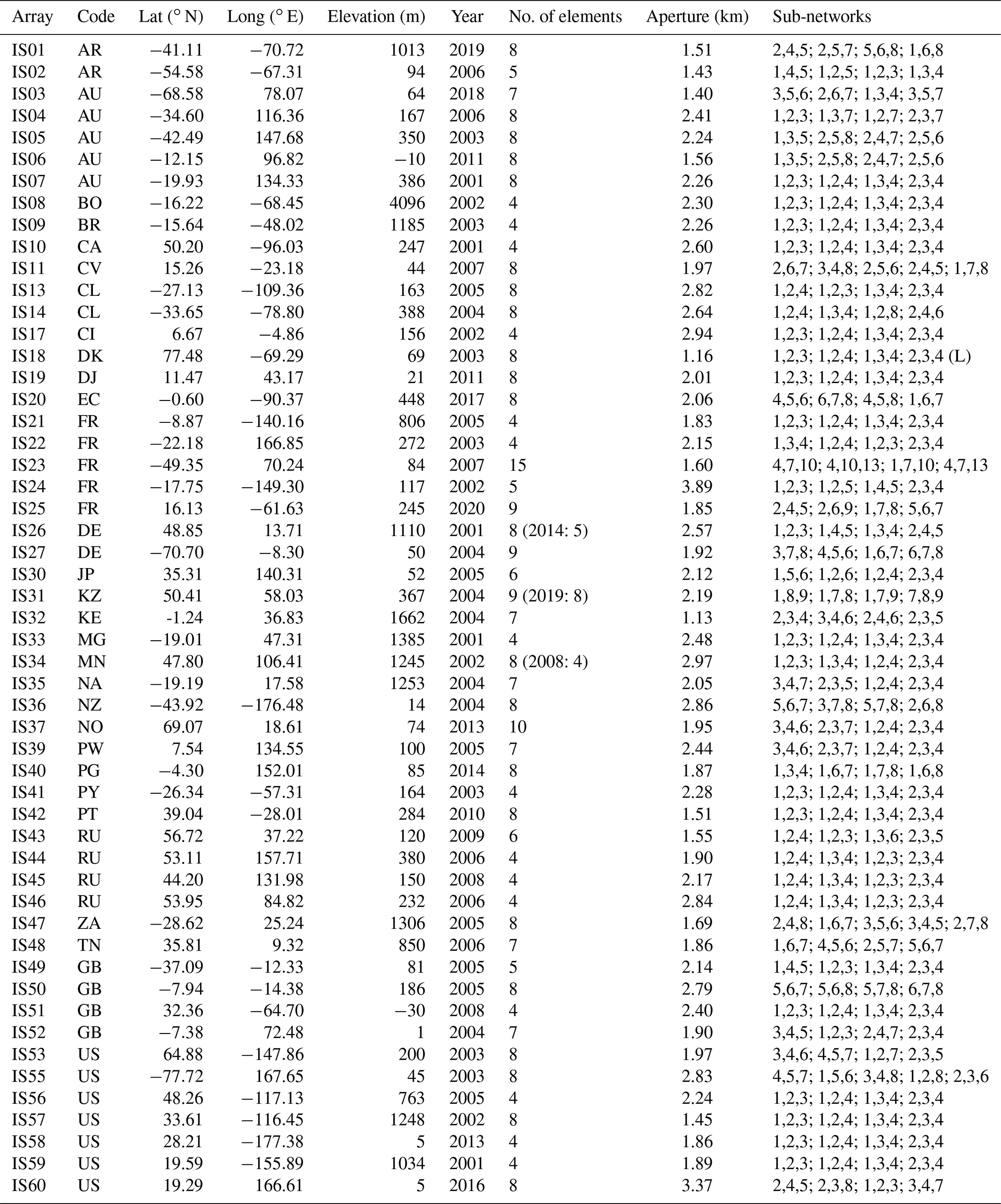
Table B1 Product availability per station (N_avail) in percent of the total number of time steps over 18 years (N_time; in parentheses). For example, an availability of 2.7 % means that signals were present for 2.7 % of the total 18 years (2003–2020). More precisely, a product is available for this portion of all time steps considered, e.g., with 30 min temporal resolution for the maw product, the number of time steps amounts to 315 600 over 18 years and 2.7 % would be 8521 time steps with detection parameters available for a station. The data availability rate thus depends on multiple factors, such as the operational time of a station, data gaps, the actual arrivals of coherent signals, and PMCC performance, to name the most relevant here.

Appendix C: Additional figures

Figure C1 As in Fig. 7 but only incorporating detections with Q>0.5.

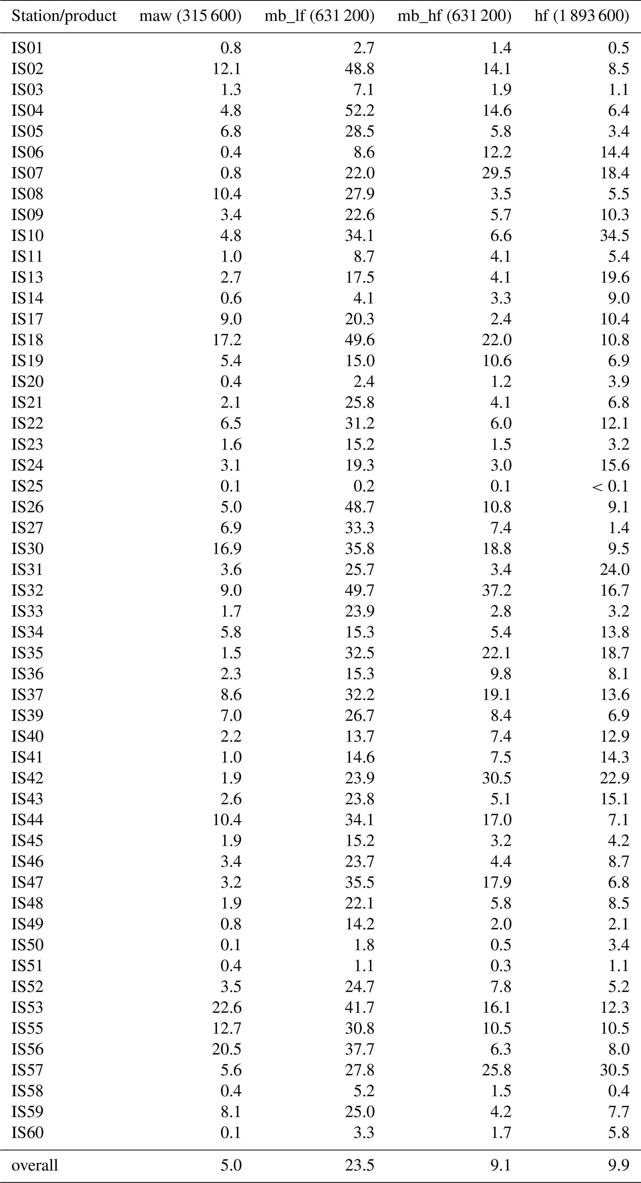
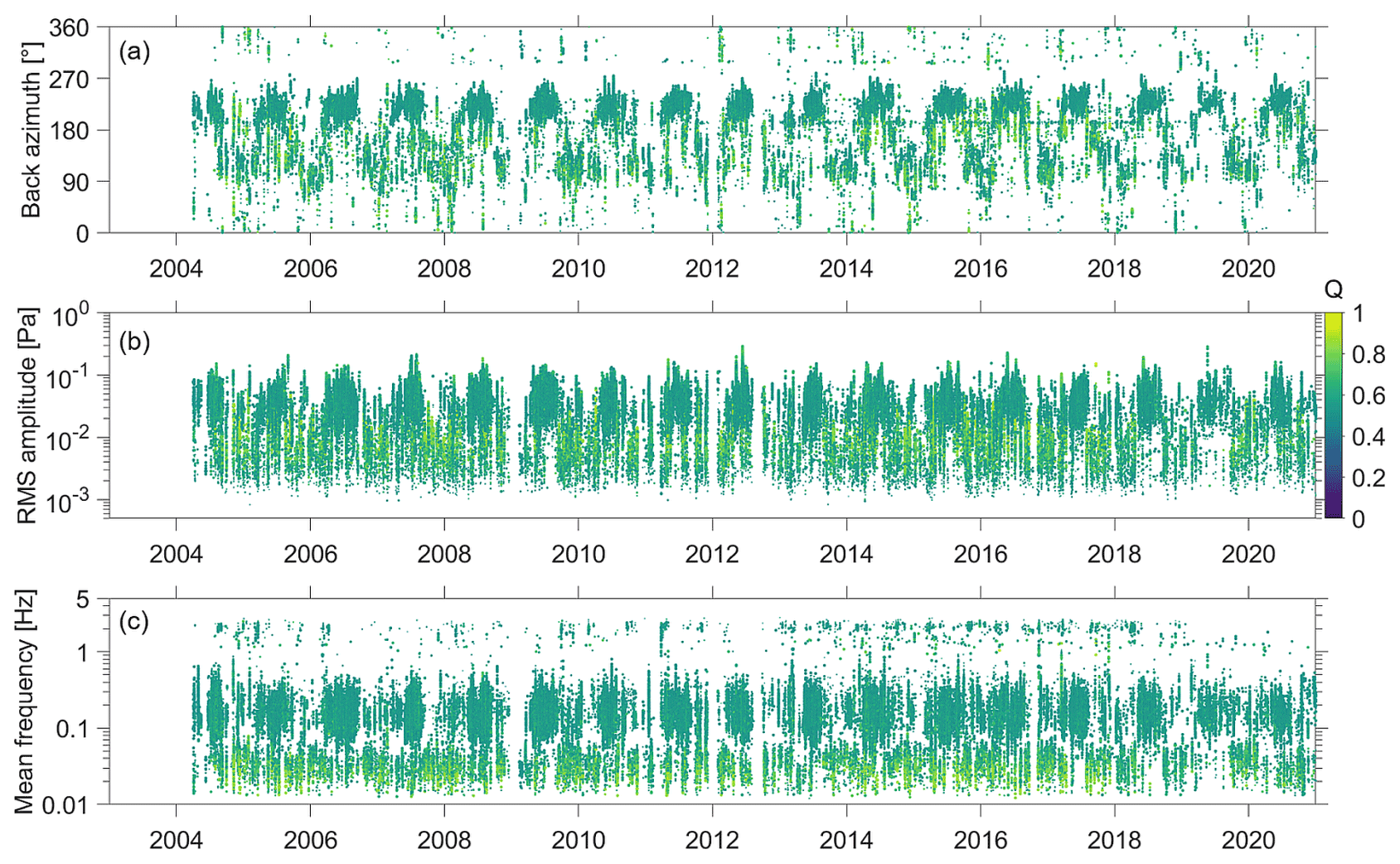
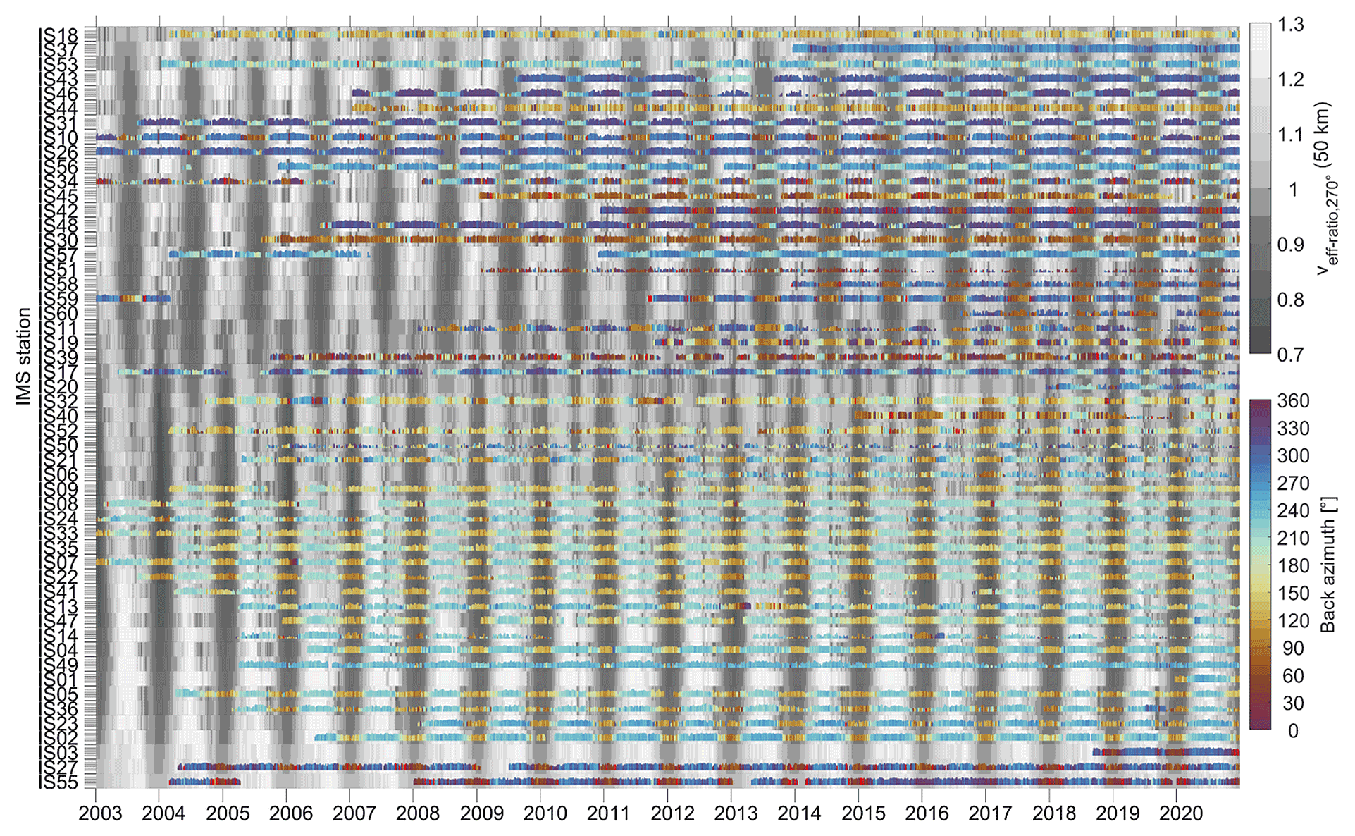
Figure C2 Similar to Fig. 11 but for the IMS infrasound detections in the microbarom frequency range (here 0.1–0.5 Hz).

Figure C3 As in Fig. 11 but for the mb_hf product (0.45–0.65 Hz). As the vertical extent of each colored line denotes the number of detections at a logarithmic scale, this global view is based on much less data than Fig. 11.

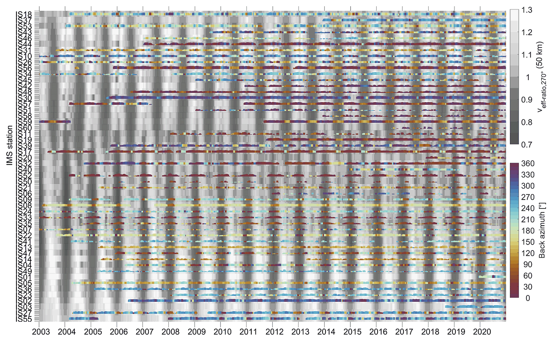
Figure C4 Similar to Fig. 13 but for the IMS infrasound detections in the maw frequency range (0.02–0.07 Hz).