A new digital lithological map of Italy at the 1:100 000 scale for geomechanical modelling

Lithological maps contain information about the different lithotypes cropping out in an area. At variance with geological maps, portraying geological formations, lithological maps may differ as a function of their purpose. Here, we describe the preparation of a lithological map of Italy at the 1:100 000 scale, obtained from classification of a comprehensive digital database and aimed at describing geomechanical properties. We first obtained the full database, containing about 300 000 georeferenced polygons, from the Italian Geological Survey. We grouped polygons according to a lithological classification by expert analysis of the 5456 original unique descriptions of polygons, following compositional and geomechanical criteria. The procedure resulted in a lithological map with a legend including 19 classes, and it is linked to a database allowing ready interpretation of the classes in geomechanical properties and is amenable to further improvement. The map is mainly intended for statistical and physically based modelling of slope stability assessment and geomorphological and geohydrological modelling. Other possible applications include geoenvironmental studies, evaluation of river chemical composition, and estimation of raw material resources. The dataset is publicly available at https://doi.org/10.1594/PANGAEA.935673 (Bucci et al., 2021).

1 Introduction

Lithology encodes information on the composition and physical properties of rocks and, therefore, it is a key variable in the study of Earth surface and subsurface processes. As such, lithological analysis is relevant to a large body of literature, including landscape evolution (Coulthard, 2001), water flow paths (Gleeson et al., 2011), landslides (Alvioli et al., 2021; Sarro et al., 2020; Reichenbach et al., 2018), chemical composition of rivers or atmospheric CO₂ consumption (Donnini et al., 2020; Gibbs and Kump, 1994; Hartmann et al., 2010), soil classification (de Sousa et al., 2020), soil erosion (Vanmaercke et al., 2021), seismic amplification (Mori et al., 2020; Forte et al., 2019), groundwater-level variability (de Graaf et al., 2017; Lorenzo-Lacruz et al., 2017), floods (Vojtek and Vojteková, 2019), oil reservoirs (Han et al., 2018), geothermal potential (Roche et al., 2019), and geomorphological classification (Alvioli et al., 2020). Lithological variability is often a measure of geological and landscape complexity and provides important information on geological evolution and heritage (Bucci et al., 2019; ISPRA and Parco Nazionale del Cilento, Vallo di Diano e Alburni, 2013; Santangelo et al., 2013), georesource settings (Bucci et al., 2016b​​​​​​​; GEMINA, 1962; Corpo Reale delle Miniere, 1926), geoenvironmental risks (Giustini et al., 2019; Bentivenga et al., 2004), and matter fluxes at the Earth's surface (Brogi and Liotta, 2011; Boni et al., 1982).

Lithological heterogeneity should therefore be sufficiently represented in maps at the local, regional, and supra-regional scales.

Lithological information is commonly derived from geological maps. In recent years, much effort has been made to make the geological data available around the world accessible at the best possible scales (Table 1, IDs 1 and 2). However, this still remains an open challenge because the quality, scale, updating, and availability of geodata vary enormously across the globe.

Table 1 Uniform resource locators (URLs) of the institutional services, guidelines, products, or datasets consulted to compile our map.

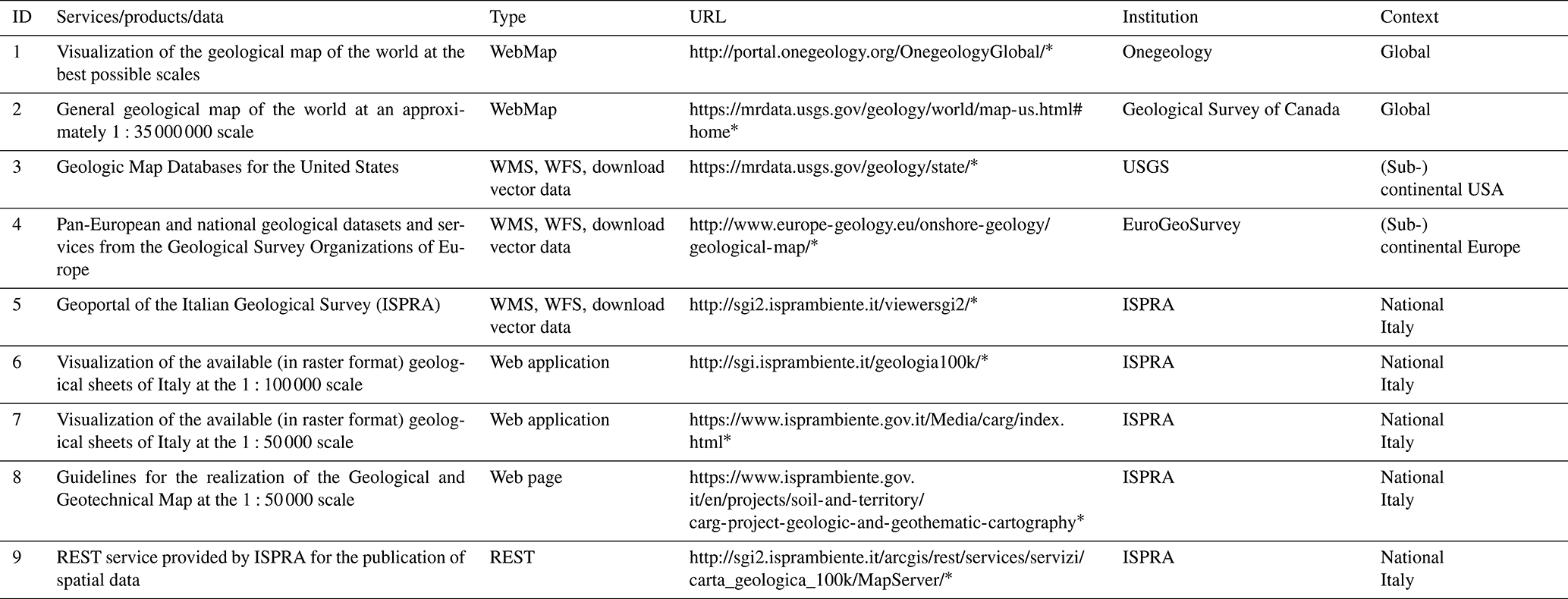
^* Last access: 25 August 2022.​​​​​​

The situation is more homogeneous at the continental or sub-continental level. For example, in 2017 the US Geological Survey published a compilation of the individual releases of the Preliminary Integrated Geologic Map Databases (SGMC) for the United States (Table 1, ID 3), which represents a seamless spatial database of 48 state geological maps that range from the 1:50 000 to 1:1 000 000 scales (Horton et al., 2017). The SGMC is not a truly integrated geological map database because geological units have not been reconciled across state boundaries. However, the geological data contained in maps for individual states have been standardized to allow spatial analyses of lithology, age, and stratigraphy.

In Europe, in 2016 EuroGeoSurvey launched the European Geological Data Infrastructure (EGDI, Table 1, ID 4). EGDI provides access to pan-European and national geological datasets and services from the Geological Survey Organizations of Europe. Geological layers available include the geological map of Europe, 1:5 000 000 scale, and the surface lithology of Europe, 1:1 000 000 scale. More detailed geological or geologically derived maps are available at national scale only (Table 1, IDs 5 and 6).

In Italy, the existing geological maps with national coverage (Console et al., 2017) are at the 1:1 250 000 (Bonomo et al., 2005), 1:1 000 000 (Pantaloni, 2011; Cipolloni et al., 2009; Compagnoni, 2004), 1:500 000 (Compagnoni et al., 1976–1983), and 1:100 000 scales (Servizio geologico d'Italia, 2004) and are managed by ISPRA (Istituto Superiore per la Protezione e la Ricerca Ambientale – Delogu et al., 2012). The 1:50 000 national geological map, coordinated and published by ISPRA, has incomplete coverage of the Italian territory (Table 1, IDs 7 and 8).

Some of the abovementioned maps are accessible, for display purposes only, via standard viewing services (WMS – Web Map Service, Table 1, ID 5).

Amanti et al. (2007, 2008) described the first known attempt by ISPRA to draft a lithological map of Italy at the 1:100 000 scale. The published map covers 65 % of the national territory and does not include Sardinia, Sicily, and the sheets 156 to 176, 183 to 187, and 196 to 199. This lithological map is not accessible in raster or vector format.

In 2018, ISPRA completed the work published in the 2007 and 2008 publications, and a lithological cartography of the entire Italian territory at the 1:100 000 scale was made accessible for visualization through the geoportal (Table 1, ID 5). The map was obtained by gathering information from the 277 sheets of the Carta Geologica d'Italia, adopting a unique legend model to produce a homogeneous lithological map of the entire country.

However, specific applications in different geoscience fields require distinct criteria and methods to elaborate different lithological classifications. For example, starting from the geological maps produced by ISPRA at the 1:100 000 scale, a geolithological map of Italy was recently classified according to the expected seismic behaviour of the material (Forte et al., 2019), although the map is only represented as a figure along the paper and is not available for download or visualization.

Here, we describe a new lithological map of Italy (LMI), entirely available for download, aimed at differentiating lithotypes based on their expected geomechanical properties in relation to slope stability and with the specific purpose of being used in statistically based (Reichenbach et al., 2018; Schlögel et al., 2018; Alvioli et al., 2016; Rossi and Reichenbach, 2016) and physically based (Alvioli et al., 2021, 2016; Mergili et al., 2014; Raia et al., 2014) slope stability models. Early versions of the map described in this work were used for geomorphological analysis and terrain classification (Alvioli et al., 2020) and for rockfall susceptibility assessment (Alvioli et al., 2021). The map and the associated database were designed in a versatile way. They can be easily enhanced/reclassified using different or additional criteria, e.g. considering age, tectonic, or geotechnical information, and thus can be relevant to a wide range of studies.

2 Data

The LMI was prepared starting from the data of the 277 sheets of the geological map of Italy at the 1:100 000 scale (Table 1, ID 6) provided by the Italian Institute for Environmental Protection and Research (ISPRA – Italian Geological Survey; Servizio geologico d'Italia, 2004), available as a digital database through the ISPRA website. The website exhibits a representational state transfer (REST) service for the publication of spatial data (Table 1, ID 9) and distributes the geological map of Italy at the scale of 1:100 000 in vector format (Fig. 1). The map contains 294 266 topologically correct polygons and 5477 unique descriptions of the geological formations. The scanned versions of the original geological sheets are also available for consultation (Table 1, ID 6).

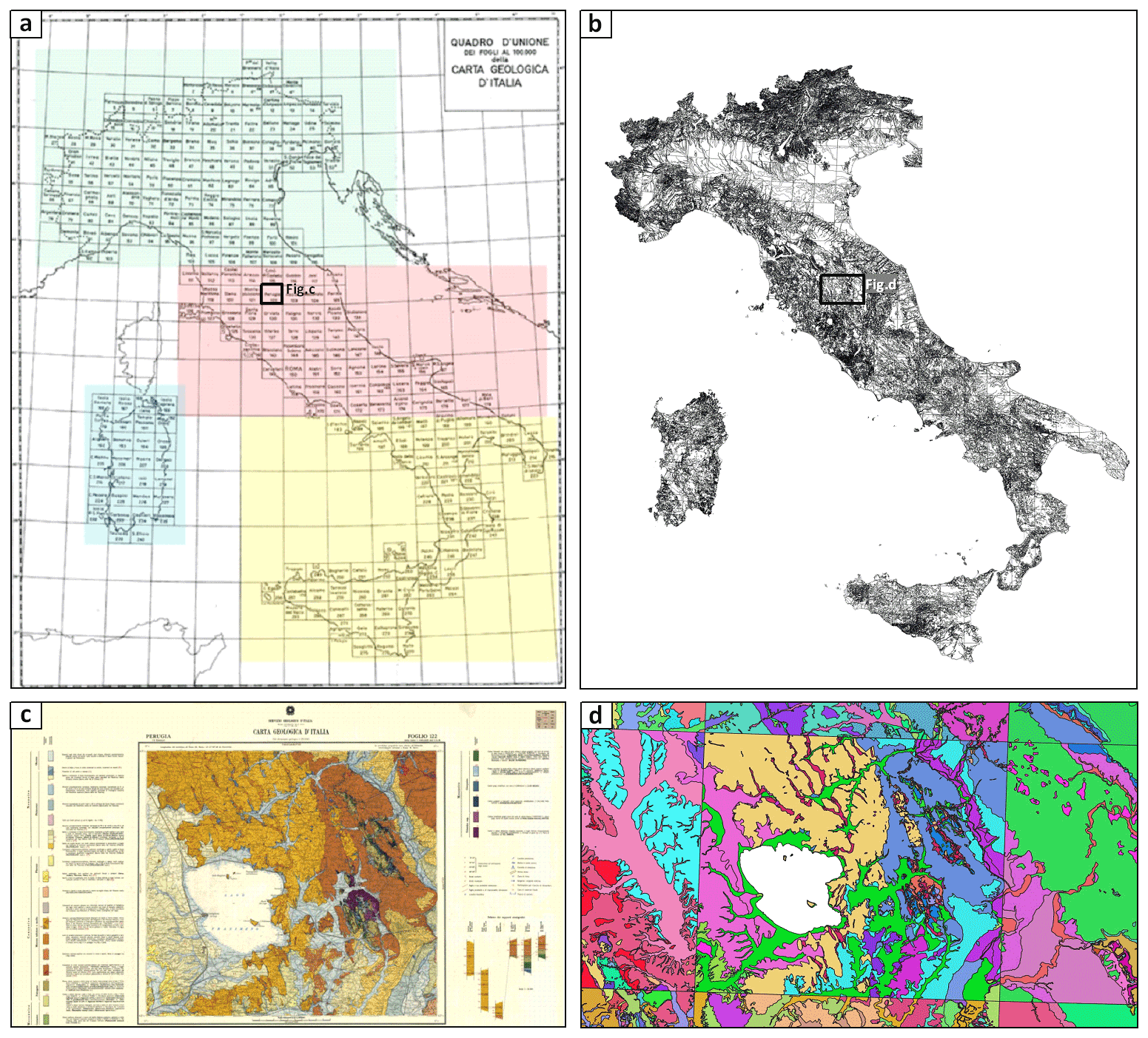
Figure 1 (a) The 277 sheets of the geological map of Italy at the 1:100 000 scale as visualized on the ISPRA website (Table 1, ID 6). The location of (c) is indicated. (b) All 292 705 unclassified vector polygons available in the source dataset. The location of (d) is indicated. (c) Published version of sheet no. 122 “Perugia” as visualized in raster form at the ISPRA website (Table 1, ID 6). (d) Randomly coloured polygons within the area encompassing sheet no. 122. Polygons with the same geological description in the original attribute table (field: NAME) provided by ISPRA (Table 1, ID 9) assume the same colour. The area also encompasses the straight boundaries with its surrounding four geological sheets, clearly visible as sharp colour changes along NS- and WE-oriented straight lines.​​​​​​​

The attribute table associated with the polygons originally contained a unique numerical identifier and the description of the geological unit as specified in the original geological maps (field: NAME). Comparison between the original legend descriptions and the text reported in the description field revealed that several simplifications were made. Such differences represented a major source of inhomogeneity within the database, which limited the efficacy of using automated database queries to apply the new lithological classification scheme. Table 2 reports examples of such simplifications of the original legend.

Table 2 Examples of simplifications and problems related to the unique rock descriptions contained in the source dataset and comparison with the original description in the legend of the original geological sheets. Depending on their nature, issues were approached using database queries (Q), spatial queries (SQ), and ancillary material (regional/local geological maps and literatures).​​​​​​​

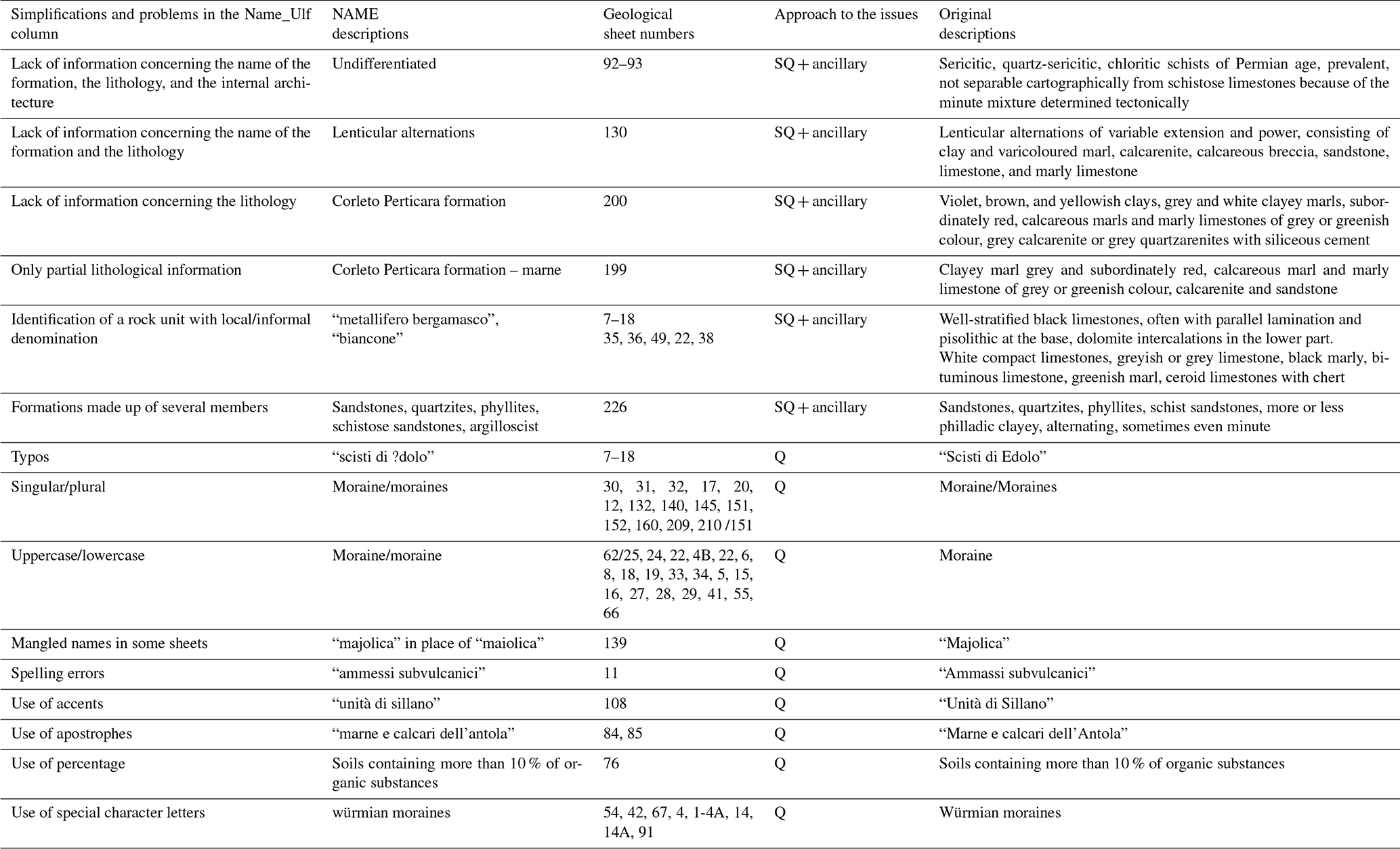
In most cases, the text corresponds only to the first word or lemma of the original description. In the case of formations made up of several members, the NAME field contains a lemma indicating the main lithological members, but this approach is not consistent for all records. In some cases, the polygons correspond to empty records in the attribute table (most of them refer to lakes or inland waters); in others, the polygons are absent and were added in this work to fill in empty areas according to the information checked in the original geological sheets. Overall, the analysis of the database revealed several types of errors affecting the source dataset, which are summarized in Fig. 2a. We refer to errors in the database as thematic errors​​​​​​​, since the attribute assigned to a polygon is incorrect or does not correspond to the ground truth (assumed here to be the original geological sheets). Thematic errors in the database can be grouped according to two main categories: inconsistency between surveyors and errors by the operators who compiled the database. We refer to the first as data acquisition errors and to the second as database compilation errors.

Data acquisition errors are related to individual mapping errors (reconnaissance errors, in Fig. 2a) or to disused or dialectal/jargon geological descriptions (semantic errors, in Fig. 2a). Figure 3a and c show typical errors related to subjectivity issues visible at the boundary between geological sheets drafted by different working groups and published many years apart from each other (Console et al., 2017). Figure 3c also contains references to local or dialectal terms that may escape general lithological classification criteria. Subjectivity errors related to disused, inadequate, or dialectal geological descriptions and terms were systematically resolved (Fig. 3d) by using database queries. Despite our efforts, little or nothing could be done for most of the errors due to contrasting classifications of rock assemblages by individual geologists or the working groups who compiled the original geological sheets. Such problems still remain in our lithological map (Fig. 3b, d). A new national geological survey currently in progress (Carg project, Table 1, IDs 7 and 8) will likely resolve critical information on geological interpretation, which is beyond the scope of this work.

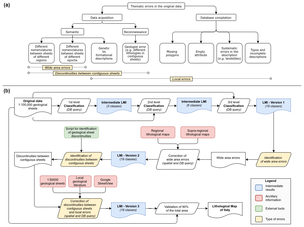
Figure 2 (a) Scheme of the main thematic errors identified in the source dataset. Errors can be related to (i) uncorrected or incomplete database compilation or (ii) data acquisition as a consequence of individual errors or inhomogeneity in the use of geological nomenclature, description, and interpretation. (b) Flowchart of the classification process of the lithological map of Italy.

Database compilation errors can be systematic (Fig. 3f) and occasional. Figure 3f refers to a systematic thematic error dealing with the compilation of the NAME column of some landslide polygons with the description of a lithostratigraphic unit clearly unrelated to landslides. As exemplified in Fig. 3f, the compilation errors were identified and corrected during the reclassification of the source dataset.

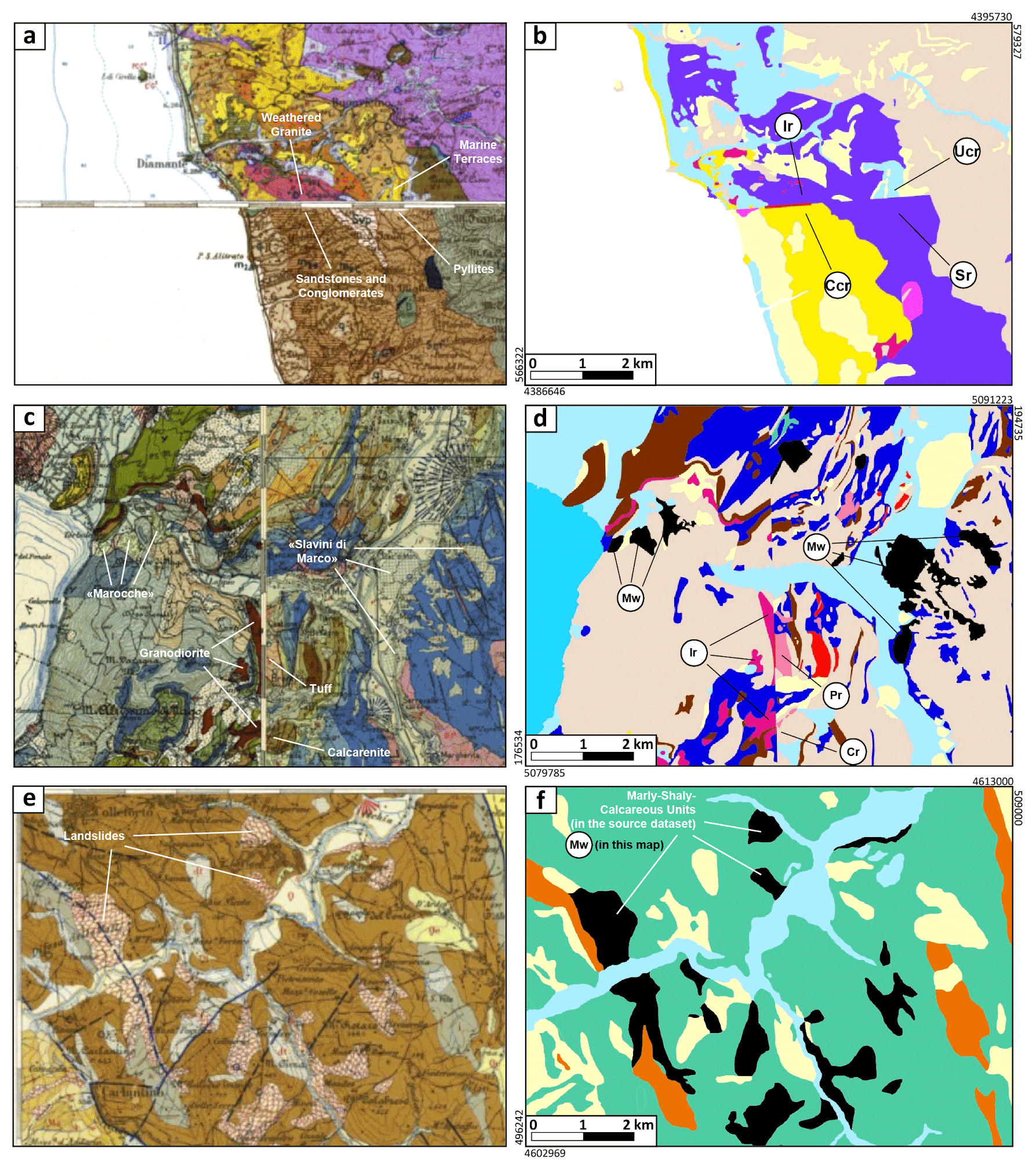
Figure 3 The main problems of the source dataset highlighted through the comparison of representative areas as they appear in the published raster version of the geological sheets (a, c, e) and in our reclassified vector map (LMI) (b, d, f). Vector map legend – Ir (intrusive rocks), Ucr (unconsolidated clastic rocks), Ccr (consolidated clastic rocks), Sr (schistose rocks), Pr (pyroclastic rocks), Cr (carbonatic rocks), Mw (mass wasting). Examples of errors related to locally wrong rock classification and inhomogeneity problems at the boundary between geological sheets of different years are shown in panel (a) (year 1969 – N sheet no. 220 vs year 1890 – S sheet no. 228) and in panel (c) (year 1948 – W sheet no. 35 vs year 1966 – E sheet no. 36). Examples of local/dialectal terms in the geological description are shown in panel (c) (“Marocche” and “Slavini di Marco” for mass wasting). Examples of errors related to incorrect database compilation are shown comparing panels (e) and (f). Panels (a), (c), and (e) include sheet nos. 220, 228, 35, 36, and 163 as visualized in raster form at the ISPRA website (Table 1, ID 6).

3 Methods

The procedure used to compile the new LMI is described in Fig. 2b. Starting from the original data (top left in Fig. 2b), we derived the LMI (bottom right in Fig. 2b) through the following steps: (a) definition of a procedure including alphanumeric queries, geospatial analysis, and expert judgements; (b) preparation of at least two intermediate products and three versions of the LMI.

The Intermediate LIM – 3 classes product (Fig. 2b) follows a genetic criterion and describes (i) magmatic, (ii) metamorphic, and (iii) sedimentary rocks.

The Intermediate LIM – 6 classes product (Fig. 2b) distinguishes (i) older (typically pre-Neogene in age) and structured substratum-derived sedimentary rocks and (ii) magmatic intrusion from (iii) younger (Neogene and Quaternary in age) less to non-deformed sedimentary and magmatic cover rocks. Sedimentary cover was further separated into (iv) undifferentiated and (v) alluvial/marine rocks, while the (vi) metamorphic rock class remains unchanged.

LMI – Version 1 (Fig. 2b) is based on a predominantly lithological criterion and contains the 19 classes defined in our legend.

To translate different rock-type information into lithological classes, the dominant rock types were emphasized assuming that the rocks mentioned foremost are more abundant than those mentioned later in the descriptions. This classification strategy is consistent with many mapping guidelines (Cohen et al., 2013; Hartmann et al., 2012; Asch, 2005) and is based on the classification system by Dürr et al. (2005) with modifications. Determining the dominant rock types within a unit was not always straightforward though. Cases of uncertainty about the dominant rock type were found and were resolved by considering specific lithological classes defined by the combination of the most representative rock types. For example, the rock unit named “clays and limestones”, composed in equal parts of both lithotypes, was assigned to the “mixed sedimentary rocks” class, which also contains other sediments where carbonates are mentioned but are not dominant.

Each classification step (“1st, 2nd, and 3rd level” in Fig. 2b) used the result of the former step (where applicable) and the original data to build complex alphanumerical database queries. No spatial queries were involved. Furthermore, the first two (coarser) levels of classification (intermediate products) helped underline systematic semantic and compilation errors throughout the database. For example, rock units containing the word “schist” were consistently classified as “metamorphic rocks” in the first-level classification, which led to classification of sedimentary rocks with a strong pelitic component as metamorphic rocks. This happened since such sedimentary rocks were commonly improperly indicated as “schists” in geological descriptions dating over 50 years. Similarly, the words “clays” and “claystones” or “sands” and “sandstones” were sometimes used as synonyms in the original geological legend, with consequent uncertainty between the sedimentary cover or the sedimentary substratum.

Inconsistencies in the source dataset mainly derive from the large variability in the level of detail of the original geological descriptions between different geological sheets. Compilation of the 277 geological sheets of the entire national territory required 92 years, from 1884 to 1976 (Fig. 4a), which inevitably led to differences in the geological descriptions (and interpretations) between old and recent sheets.

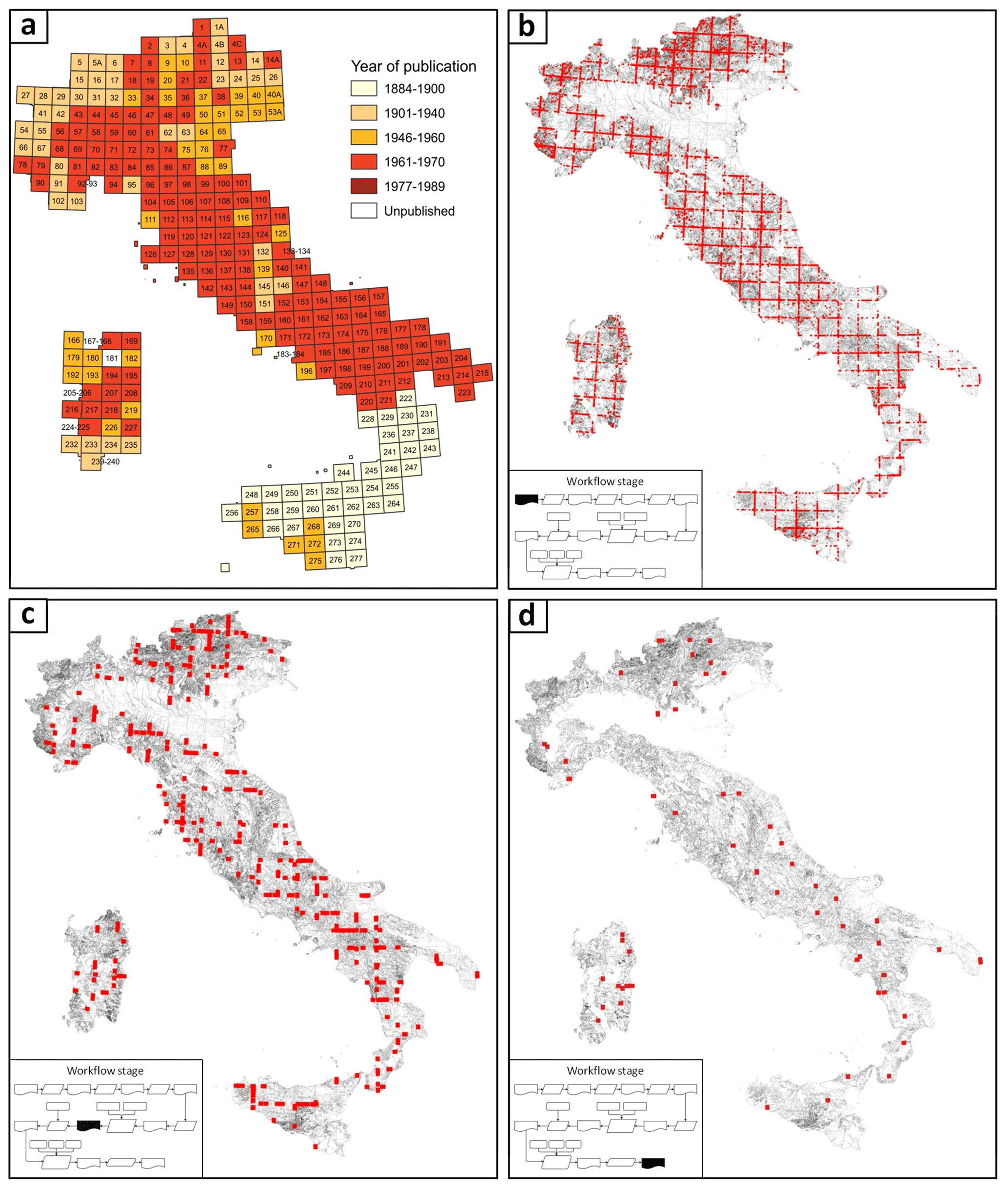
Figure 4 (a) The 277 sheets of the geological map of Italy at the 1:100 000 scale classified according to the years of publication, as visualized in Console et al. (2017), Fig. 3. (b) The 12 711 NS–EW-oriented segments (red lines) with different lithotypes in the two sides and sinuosity equal to 1. (c) The 405 red lines longer than 1000 m left after semi-automatic classification. The 294 266 unclassified vector polygons of the source dataset are shown as background in panels (b) and (c). (d) The 58 red lines longer than 1000 m left after the expert analysis of the semi-automatic output. The 100 705 unclassified vector polygons derived from the dissolve GIS operation performed after the classification phase are shown as background. Insets in panels (a), (b), and (c) indicate the classification stage to which each map refers, according to the scheme in Fig. 2b.

A similar issue was introduced between sheets or regions mapped by different authors and working groups (Fig. 3a, c). As a consequence, problems of inhomogeneity were found in the descriptions of lithostratigraphic units, which in turn generated problems of harmonization at the boundaries between different geological sheets. To mitigate inhomogeneity problems, we decided to adopt broad categories in the classification of the third level as a function of similar lithologies, genetic processes, and expected geotechnical behaviour. With this aim, rock descriptions were generalized into 19 lithological classes. However, harmonizing the 5477 original univocal descriptions of the geological units into 19 simplified lithological classes was often tricky and required expert judgement supported by the consultation of regional and supra-regional geolithological maps (Conti et al., 2020; Piana et al., 2017; Lentini and Carbone, 2014; Carmignani et al., 2013; Vezzani et al., 2010; Celico et al., 2007; Carmignani, 2001; Boni et al., 1982; Bigi et al., 1993; Amodio-Morelli et al., 1976). We used a very long and complex set of database queries to classify and harmonize the data. For example, to correctly classify glacial drift, avoiding possible overlapping with alluvial deposits, we requested the NAME field to contain strings with the words “wurm”, “würm”, “glacial”, and “moraine” and at the same time without any of the words “alluvial”, “fluvial”, and “terrace”. Due to their specificity, queries were generally longer and more complex when used to classify widespread lithological classes containing a large number of unique descriptions. LMI_Version 2 is the product of this harmonization phase where “wide-area errors” were corrected (Fig. 2b), resulting in a lower number of discontinuities at the boundaries of regions or individual geological sheets compared with those contained in LMI_Version 1 (Fig. 4b, c).

To identify discontinuities between contiguous geological sheets (Fig. 2b), we developed an automatic procedure based on the analysis of the lithological classes located to the right and left of each lithological boundary. We selected all EW- and NS-oriented straight boundaries longer than 1 km and resolved classification inconsistencies across such boundaries through expert advice. Discontinuities between contiguous geological sheets are due to inconsistencies between surveyors. Since we assumed that the ground truths are the original geological sheets, our approach consisted in assuming only one of the two contiguous polygons was to be corrected. If available ancillary data allowed us to confirm one of the two bounding polygon attributes, classification of the second polygon was amended accordingly. Otherwise, the discontinuity was solved by assigning the class that minimized discontinuities and inconsistencies.

To reduce the number of discontinuities between contiguous sheets, we consulted geological maps available at the 1:100 000 scale (Servizio geologico d'Italia, 1970a, b, e, d, c, 1969, 1968a, b, 1965, 1955; Regio Ufficio Geologico, 1884a, b, c, d, e; Servizio geologico d'Italia, 1964; Ministero dei Lavori Pubblici, Ufficio Idrografico, Sezione Geologica, 1948) and at the 1:50 000 scale (Servizio geologico d'Italia, 2016, 2015b, c, a, 2014, 2012c, a, b, 2011c, b, d, a, 2010b, c, a, 2009a, b, 2008, 2006, 2005c, b, a, d, 2002, 1972, 1977) where available. Where information on rock types was unavailable from the national maps, we obtained the descriptions of the named stratigraphic units from regional and local geological maps and from the scientific literature (Novellino et al., 2021; Bucci et al., 2020, 2016b, 2014, 2012; Vignaroli et al., 2019; Mirabella et al., 2018; Ronchi et al., 2011; D'Ambrogi et al., 2010; Brozzetti, 2007; Chiarini et al., 2008; Giannandrea et al., 2006; Schiattarella et al., 2005; De Rita et al., 2004; Girotti and Mancini, 2003; Catanzariti et al., 2002; Bortolotti et al., 2001; Prosser, 2000; Giardino and Fioraso, 1998; Tavarnelli, 1997; Campobasso et al., 1994; Centamore et al., 1991; Patacca et al., 1991; Calamita et al., 2009; Centamore et al., 2009; Gueguen et al., 2010; Tavarnelli et al., 2003b, a). The quality of the literature was variable and may have introduced some uncertainty. In some rare locations, the rock-type information of digital geological map vector datasets was derived from paper maps, which were georeferenced and visually assigned to the units of the digital maps. In specific and rare cases, it was necessary to use geographic visualization software, such as Google Earth and Google Street View, to study and display images of outcrops for a local visual analysis. After this finer phase of correction, a total of 58 segments longer than 1000 m remained unsolved since they would require the geometry of the original polygons to be modified (Fig. 4d). The problem greatly increases for the classification inconsistencies along segments shorter than 1000 m, for which a systematic correction was beyond the scope of this work.

After the classification phase, boundaries were dissolved to merge adjacent polygons sharing the same lithology. With this streamlining operation, the number of polygons dropped from 294 266 to 180 503. The result of the correction of discontinuities between contiguous sheets is LMI_Version 3 (Fig. 2b).

Eventually, we performed a validation of the map of LMI_Version 3 (Fig. 2b). First, the area percentages of all the unique descriptions within each class were computed and sorted in descending order. Then, within each lithological class, all the unique descriptions summing to a total area of 90 % of that class were inspected for possible inconsistencies by comparing and verifying the assigned lithology with the original description in the NAME field. The total area validated corresponds to 271 651.56 km², which represents ∼ 90 % of the Italian territory and includes 1702 different geological descriptions. For each lithological class, polygons of a very small size, between 0.05 % and 0.8 % of the area of the lithological class itself, were validated (Table 3). The remaining 10 % of the total area of each lithological class, which consists of 4632 records associated with negligible percentage values of the area (on average ​​​​​​​0.06 % of the total area of each class), was not checked. It is worth noting (Table 3) that the carbonate rock class (Cr) accounts for most of the descriptions (1155), followed by unconsolidated clastic rocks (Ucr), alluvial and marine deposits (Al), and siliciclastic sedimentary rocks (Ssr), which include 856, 583, and 560 descriptions, respectively. However, the areal extent of these four classes (the most represented in the territory) does not reflect the number of descriptions, as the most extensive class is Al (75 424.36 km²), followed by Ucr (45 764.12 km²) and then Cr and Ssr (45 329.81 and 34 099.68 km², respectively).

We checked all of the records classified as anthropogenic deposits (12 records), landslides (26 records), and lakes and glaciers (10 records) (Table 3). Some errors inherited from compilation errors of the source dataset also emerge from the validation as classification inconsistencies. To give an example of this kind of error, we report a case from the landslide class in which the most representative (21 % of the area, with respect to the total landslide class) unique descriptions are defined as “clayey and calcareous turbidites of Paleogene age”. These same polygons were, instead, correctly represented as landslides in the original geological sheet in raster format (Fig. 3e). Wherever possible, polygons classified as landslides were manually corrected by looking at the original raster map. Similar errors concerning other geological descriptions were treated using the same approach. After validation, the final LMI was produced (Fig. 2b).

Table 3 Descriptive statistics of the 19 lithological classes. In the left half of the table, the number of polygons and their minimum, maximum, average, and total area for each lithological class are shown. The right half of the table shows the number of total unique descriptions and those checked during the technical validation in relation to the percentage of the area covered by the validation (% of the total area) and the detail of the validation (minimum area checked).

4 Results

The main results of this work are (i) the translation of the rock-type information extracted from the stratigraphic units of the geological maps of Italy at the 1:100 000 scale into lithological classes and (ii) the development of a data architecture open to further improvement, aimed in particular at linking the lithological classes to their expected geotechnical behaviour.

The new LMI (this work) represents the first freely downloadable national distribution of the different lithological classes at a high resolution. The dataset is publicly available at https://doi.org/10.1594/PANGAEA.935673 (Bucci et al., 2021). The map scale is 1:100 000. The assembled map consists of a total of 180 503 polygons distributed in 19 lithological classes (Fig. 5).

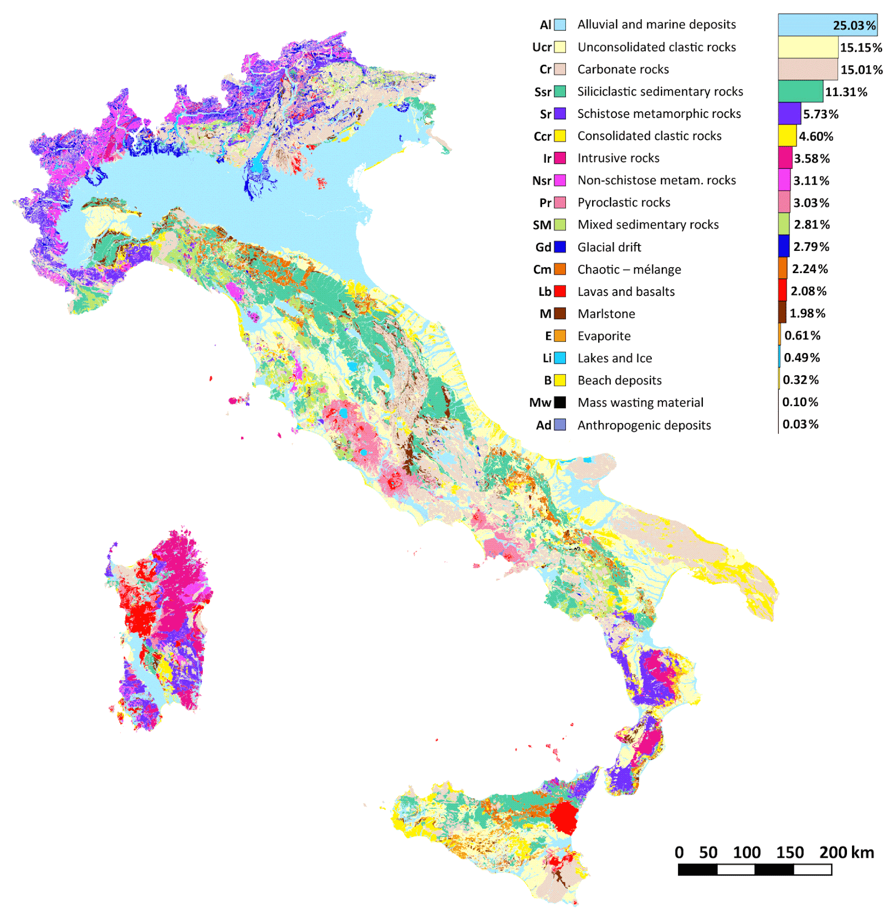
Figure 5 Map of Italy showing the 19 lithological classes identified with both the short ID and the extended name.

The percentage distribution of each lithological class over the Italian territory is indicated and visualized in a bar chart.

The Italian surface is covered by ​​​​​​​82.47 % sediments (a third of which are alluvial deposits), 8.84 % metamorphics, 3.58 % plutonics, and 5.11 % volcanics (Table 4). A specific class was assigned to areas of ice and inland water bodies, which cover 0.49 % of the map area.

Table 4 Percentage distribution of the lithological classes (columns), organized into three hierarchically different levels of classifications within the 18 physiographic regions of Italy (rows).

Below, the lithological classification describes the general rock types in each unit in alphabetic order.

• Alluvial deposits (Al): alluvial, lacustrine, swamp, and marine deposits. Eluvial and colluvial deposits.

• Anthropogenic deposits (Ad): include Roman and modern landfills, drainage channel excavations, and archaeological remains.

• Beaches and coastal deposits (B): include beaches and coastal deposits.

• Carbonate rocks (Cr): carbonate-dominant sedimentary rocks. Examples of Cr units are limestone, dolomite, and marl (but only where associated and in a clear minority with respect to limestone; otherwise, they are included in class M). As usual, the rock descriptions of the mapped units do not give the relative abundances of the rock types which they encompass: units were classed as Cr if the first named rock type was a carbonate rock, if the majority of rock types were carbonates, or if the named order otherwise led to the impression of a domination by carbonates.

• Chaotic – mélange (Cm): includes chaotic terrains with a predominantly clay matrix and olistostromes composed of mixed sedimentary rocks (SM class). Fragments of ophiolite structures were locally included in the Cm class.

• Consolidated clastic rocks (Ccr): clay, sand, debris, and conglomerates of a varied origin, usually of Neogene and Quaternary age, which have undergone consolidation or secondary cementation phenomena.

• Evaporite (E): contains substantial amounts of evaporitic rocks. The typically and most frequently encountered evaporite rock is gypsum, but anhydrite and halite are also present. If a map unit was interpreted as dominated by evaporites, it was classified as E, regardless of other mentioned rocks. This implies that the E class may additionally contain e.g. carbonates.

• Glacial drift (Gd): includes moraines and other related deposits.

• Intrusive rocks (Ir): acid (granites, quartz diorites, quartz monzonites), intermediate (diorite, monzonite, syenite), and basic (gabbro and peridotite) plutonics. Ophiolite structures are included in the basic plutonic except for basalt (Lb class) and serpentinite (Sr class).

• Lakes and ice (Li): lakes, rivers, ice, and glaciers on some Alpine mountains. However, the coverage is not representative of lake or ice extent, as the priority of this map is lithology.

• Lavas and basalts (Lb): volcanic rocks including acid (rhyolites, trachytes, or dacites), intermediate (andesites), and basic (basalt-type rocks, tephrites, tholeites, and lamprophyres) volcanics.

• Marlstone (M): includes mostly marly rocks with a composition ranging from calcareous marls to clayey limestones. Typically, it contains marly sediments of cartographic importance associated with carbonatic rocks (Cr) or siliciclastic sedimentary rocks (Ssr).

• Mass wasting material (Mw): includes landslides.

• Mixed sedimentary rocks (SM): sediments where carbonate is mentioned but is not dominant. The class encompasses mixed sedimentary rocks that are usually a combination of different rock types (e.g. interlayered sandstone and limestone or shaley marl with interlayered subordinated calcilutite beds or radiolarite). Mixed pelagic sediments as well as calcareous turbidites are included in the SM class.

• Non-schistose metamorphic rocks (Nsr): metamorphics where the schistose fabric can be present but not dominant. It contains gneiss, amphibolite, quartzite, meta-conglomerate, and marble.

• Pyroclastic rocks (Pr): sediments of volcanic origin. Typical pyroclastics are tuff, volcanic breccias, ash, slag, pozzolan, and pumice.

• Schistose metamorphic rocks (Sr): a “broad” lithological class that encompasses a wide variety of rocks from phyllite to schist, including association of schist and paragneiss. Ophiolite-derived rocks that show a certain degree of metamorphism and schistosity (e.g. serpentinite) are included in this class.

• Siliciclastic sedimentary rocks (Ssr): sandstone, mudstone, and greywacke. Where carbonate was named in the rock description of the mapped unit, the lithological classes Cr or SM were used, so siliciclastic sedimentary rocks are without a mapped carbonate influence. Note that in some cases the carbonate presence (e.g. as a matrix) may not be named in the rock description and siliciclastic sediments may still contain carbonates in nature.

• Unconsolidated clastic rock (Ucr): young, not yet consolidated, and/or weathered sediments, usually of Neogene and Quaternary age. It comprises all grain sizes with a heterogeneous origin loosely arranged and not cemented together. Examples of unconsolidated sediments are clay soil, sand, non-cemented breccia, loose debris, and conglomerate.

Significant regional differences in the distributions of lithologies exist (Fig. 6a, b, c, Table 4).

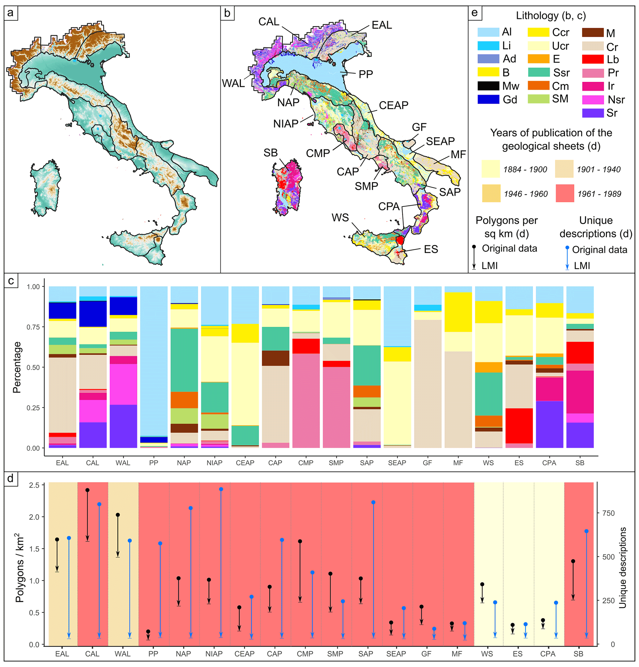
Figure 6 (a) Physical map of Italy subdivided into 18 physiographic regions. (b) Geographical distribution of the 19 identified lithological classes in the 18 physiographic regions of Italy (see Table 4 for spelling out of the acronyms). (c) Percentage distribution of the 19 lithological classes in each physiographic region. (d) Polygon density (black symbols) and number of unique descriptions (blue symbols) in each physiographic region considering the original data (points) and the LMI (arrow tips) and taking into account the years of publication of the geological sheets. (e) Legend. See Fig. 5 for the extended lithological legend.

With the exception of flat and low-lying areas of Italy, where alluvial deposits and loose clastic deposits dominate (e.g. PP), the map shows a high regional lithological variability. In WAL, metamorphic rocks dominate, while in the eastern Alps (EAL), carbonate rocks prevail. Intermediate percentages are recorded in CAL, where the metamorphic rocks to the N–NW and the sedimentary rocks S–SE are separated by an important tectonic lineament. The northern Apennines (NAP) are mainly composed of siliciclastic rocks and subordinately of chaotic and mixed sedimentary rocks, while the central Apennines (CAP) mainly consist of carbonate rocks. Intermediate percentages of carbonate rocks, mixed and chaotic sedimentary rocks, and siliciclastic deposits are found in the northern–internal Apennines (NIAP), in the southern Apennines (SEAP), and in western Sicily (WS). In WS significant percentages of evaporites are also recorded. In the central and south-eastern Apennines (CEAP and SEAP), high percentages of unconsolidated and consolidated clastic rocks are present, while carbonate rocks dominate the lithology of the Gargano Foreland and the Murge Foreland (GF and MF). The similarity between the most represented lithological classes in the Calabro-Peloritano Arc (CPA) and Sardinian Block (SB) is evident, although schistose rocks prevail in the CPA, while intrusive rocks prevail in the SB. Volcanic rocks are extensively represented in the Central Magmatic Province and Southern Magmatic Province (CMP and SMP), in eastern Sicily (ES), in the SB, and subordinately in the EAL.

Significant regional differences in the representation of lithologies also exist (Fig. 6d). In the original geological dataset, the number of polygons per square kilometre (black points in Fig. 6d) used to represent the lithological variability is strongly heterogeneous across Italy and is proportional to the geolithological complexity of each physiographic region. For instance, the Alpine regions (EAL, CAL, WA), which are characterized by a complex geological architecture and by a very high lithological variability, display the higher polygon density, with values between ​​​​​​​1.7 and 2.4 polygons per square kilometre. On the other hand, the Po Plain (PP) records the lowest polygon density, with ​​​​​​​0.2 polygons per square kilometre being characterized by a quite monotonous surface geology almost totally represented by alluvial deposits. Accordingly, in the Apennine regions, which are (in general) geologically less complex than the Alpine regions, the average polygon density is just over 1 (NAP, NIAP, CAP, SMP, SAP), with a maximum of 1.7 in the CMP and a minimum of 0.3 in the south-eastern regions of the foredeep (SEAP) and foreland (MF) domains.

The reclassification of the original geological dataset in the LMI classes determined the merging of adjacent polygons exposing rock units included in the same lithological class. The process resulted in a drop in the number of polygons in each physiographic region passing from the original dataset to the LMI, which is indicated by the length of the black arrows in Fig. 6d. Importantly, the reduction in the number of polygons does not change the relative regional variability of the polygon density. This means that the simplification introduced by our reclassification does not impact the regional difference in the representation of the lithology.

In Fig. 6d, the indicator of polygon density (in black) is flanked by an analogue indicator (in blue) displaying the count of the unique descriptions used within each physiographic region, both in the original dataset (blue points) and in the reclassified LMI (blue arrow tips). The number of unique descriptions is generally proportional to the polygon density, but cases of exceptionally high numbers of unique descriptions (e.g. PP, NAP, NIAP, SAP) are common. Primarily, this is the effect of individual geologists or working groups using several local names to define the same rock unit, thus increasing the number of unique descriptions.

Finally, Fig. 6d shows that regional differences in the representation of lithologies may also be related to the different years of publication of the geological sheets encompassed in each region. Figure 6d shows that (i) the geological sheets encompassed in the Alpine region have been surveyed in the 1901–1940 (EAL, WAL) and 1961–1989 (CAL) time intervals, (ii) almost all the geological sheets encompassed in the regions of the Italian Peninsula (PP, NAP, NIAP, CEAP, CAP, CMP, SMP, SAP, SEAP, GF, MF) have been surveyed in the 1961–1989 time interval, such as those of the SB, and (iii) the geological sheets of WS, ES, and the CPA have been surveyed in the 1884–1900 time interval. While it is not clear whether the publication years of the geological sheets play a role or not in controlling the polygon density in the Alpine regions, the impact of the different years of publications on the representation of the regional lithological variability is dramatic when comparing CPA and SB. In fact, despite a similar lithological composition (Fig. 6c) and a pre-Alpine common geological history (Alvarez and Shimabukuro, 2009), CPA and SB are characterized by a very different density of polygons (​​​​​​​0.3 polygons per squared kilometre for CPA and 1.3 for SB) due to strong differences in drafting geological sheets published almost 100 years apart from each other.

5 Discussions

The main challenge in developing a categorized lithological map lies in balancing accuracy and complexity and still properly representing the diversity of lithological variables using a limited yet reasonable number of classes to ensure ready interpretation and applicability of the map. We maintain that the 19 classes defined here allow us to optimize the use of the map for several applications, with a focus on landslide modelling. Despite the specific goals of this work, we applied a classification that can be reconciled with the ones adopted in global lithological databases (Table 1; Hartmann et al., 2012; Geological Survey of Canada, 1995) emphasizing the dominant rock types. Furthermore, information on the physical characteristics of the dominant rock types available in the original geological legend were used to define specific lithological classes.

For example, metamorphic rocks were split into two broad classes considering the dominant presence of schistose or non-schistose rocks, i.e. according to expected – or unexpected – pervasive planar anisotropies within the rock bodies. Similarly, the classes of consolidated and unconsolidated clastic sediments, in our map, consist of two separate classes according to their expected different geotechnical behaviour. In both cases, differences in physical features (e.g. schistose/non-schistose, consolidated/unconsolidated) may impact the landslide susceptibility of genetically similar rocks (Bucci et al., 2016a), hence justifying the need for these lithological classes for our scope.

We also included the marlstone class, quite unusual for generalized lithological characterization at the national scale. The need for this class arises from the systematic occurrence of significant marl interbeds within carbonate or siliciclastic rocks, whose representation highlights the cartographic detail of the map. Moreover, it is widely recognized that marl intercalations represent important geohydrological and mechanical discontinuities within rock bodies (e.g. see Peacock et al., 2017) often promoting landslide phenomena (Guzzetti et al., 1996), which is a relevant issue for our purpose. Since our map is designed to be used for landslide studies and modelling, we also decided to maintain the “landslides” class, although it covers only ​​​​​​​0.1 % of the Italian territory. We are aware that this percentage value is strongly underestimated. The Inventory of Italian Landslides (Trigila et al., 2010), still incomplete, counts over 620 000 landslides covering a total area equal to 7.9 % of the Italian territory, and the occurrence of the different types of landslides gives rise to very different patterns of landslide susceptibility, consistent with the diverse lithological formations (Loche et al., 2022). However, we acknowledge that the large difference in percentage values stems from the fact that many efforts in landslide mapping have been made in recent decades, when the 277 sheets of the geological map of Italy at the 1:100 000 scale were already published.

Despite the usage of very specific lithological classes helping reliable classification of the rock types, the map is still subject to uncertainty considering rock properties of some broad lithological classes. This is highlighted, for instance, by the considerable amount of mixed limestone, marls, and shale sediments (5 %), including the chaotic (2.2 %) and mixed sedimentary (2.8 %) classes. Despite carbonate rocks and siliciclastic rocks behaving differently for a large range of physical or chemical properties (e.g. weathering processes, dissolution rates, or aquifer characteristics), they often occur “mixed” in these two geolithological classes, further indistinguishable at the scale of the used maps here.

An additional source of uncertainty remains at the boundaries of the geological sheets, where only discontinuities between contiguous sheets longer than 1 km were resolved, with the exception of 58 segments over the entire national territory. Table 5 represents a contiguity matrix for these 58 segments. Table 5 reveals that 19 segments, 33 % of the total, bound polygons pertaining to the Al (alluvial and marine deposits) class, which is the most represented lithological class at the national scale, covering 25 % of the entire national territory. The segments that bound lithological classes belonging to the same genetic groups (metamorphic, magmatic, sedimentary) total 24, 10 of which separate lithological classes of the sedimentary substratum from others belonging to sedimentary covers. Only 15 segments bound lithological classes belonging to different genetic groups. Despite all these segments representing identical inconsistencies from a graphical point of view, their potential negative local effects on the map reliability may be different from a lithological point of view. For instance, for landslide studies, we can consider negligible the potential negative effects of unrealistic, linear lithological boundaries of polygons pertaining to the Al class since they cover (almost) only flat areas of fluvial, alluvial, and coastal plains, where landslides are unexpected.

Table 5 Contiguity matrix showing the number of 58 N–S- and E–W-oriented straight segments longer than 1000 m which bound each lithological class.

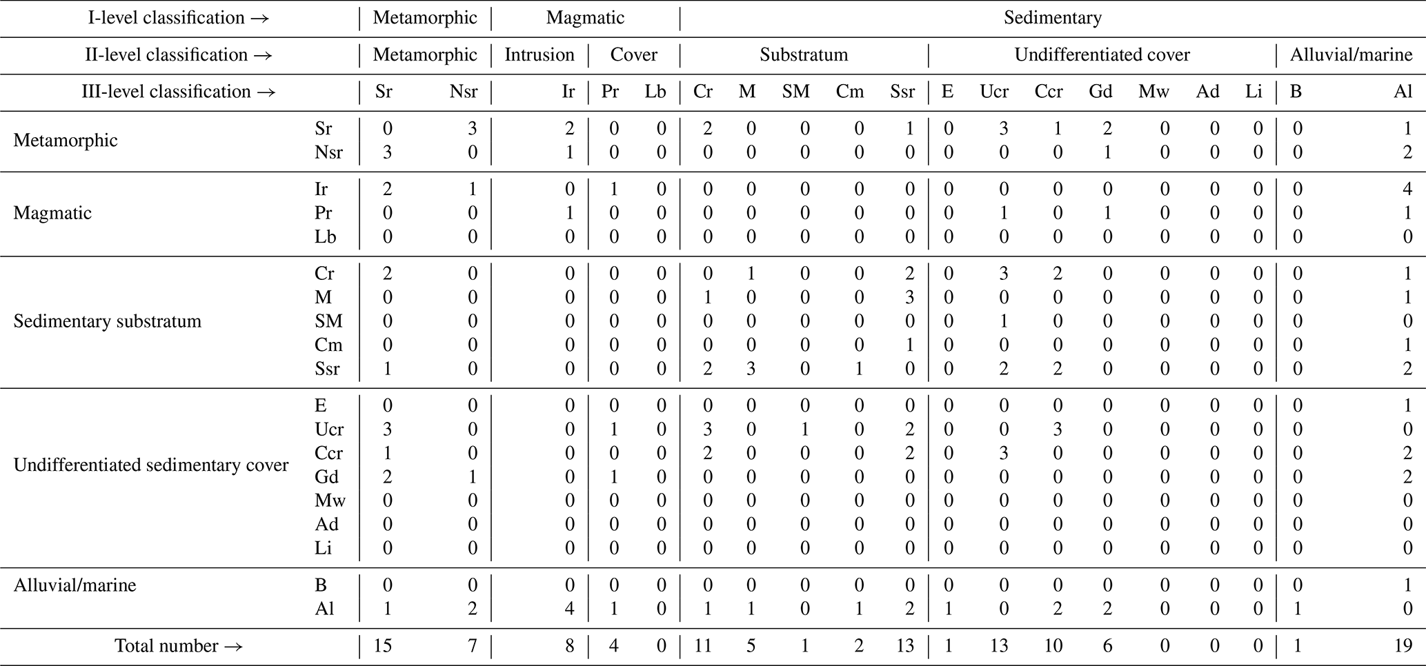
On the other hand, critical differences remain between rocks pertaining to the same genetic group but characterized by different physical properties (schistose/non-schistose metamorphic rocks, consolidated/unconsolidated sedimentary clastic rocks). Overall, we consider to be resolved the inhomogeneity problems at the boundaries between adjacent geological sheets for segments equal to or greater than 1000 m, hence considering the remaining 58 segments longer than 1000 m listed in Table 1 to be acceptable and/or negligible exceptions. Since in cartography the admissible error is traditionally assumed to be 1 mm, we maintain that, only along the boundaries of the geological sheets, our map is formally correct at the 1:1 000 000 scale, while elsewhere the cartographic detail remains compatible with the 1:100 000 scale. Pushing harmonization operation into more detail would require altering the original data, which is beyond the scope of this work.

The design of the LMI allows for further corrections and inclusion of additional information (e.g. age information, tectonic history, geotechnical properties, fine–coarse grain size ratio) in future versions, customizable for different usages, with an expected reduction in general and/or specific uncertainties. Additional information may be organized into more detailed classification levels, although their compilation will require further efforts to collect data from local geolithological literature and site-specific investigations.

Since different purposes impose different generalization strategies, other lithological classifications of the Italian rocks are possible, starting from the same source dataset. For instance, aiming at a seismic soil classification of Italy, Forte et al. (2019) generalized the lithology of Italy using 20 classes, a number comparable with the 19 classes presented here. In the Forte et al. (2019) classification, a relevant distinction was based on the identification of geolithological complexes such as geological bedrock versus those representative of cover deposits, being the last category directly related to defined values of V_S (average speed of propagation of shear waves) and hence particularly relevant for their purpose. On the other hand, the most recent lithological map of Italy provided by ISPRA as a web service is accompanied by a complex legend articulated in 48 classes aimed at describing the age, genesis, and chemical–physical characteristics of rocks, focusing on a comprehensive geological rock characterization without a specific applicative purpose. It is evident that different classifications allow different possible usages of the same original dataset; hence, at the same representation scale, different lithological characterizations can be more or less suitable, depending on the intended purpose.

Although the general rock composition of the Italian surface is remarkably similar between the existing digital lithological maps (Table 1, ID 5), the representation of the rock distribution varies largely between them and has been greatly improved in the present map, especially across geological sheets. Compared with smaller-scale maps (Compagnoni et al., 1976–1983), the main improvements lie in a better representation of complex geological settings. Moreover, a better lithological harmonization along the borders of the original geological sheets distinguishes our map from other maps at the same scale (Servizio geologico d'Italia, 2004). Figure 7 shows examples for the Sicily, Campania, and Lombardy regions, highlighting the general improvement of the map regardless of the geographical location and geological and geomorphological settings. However, a direct comparison of the maps is difficult due to the different legends (e.g. based on geological processes or lithology or mixing-up processes and lithology).

Early versions of the LMI presented here were already used to validate the terrain classification of Italy (Alvioli et al., 2020) and to estimate soil parameters for physically based rockfall modelling along the Italian railways (Alvioli et al., 2021). Such versions of the map included a few of the inconsistencies resolved in this work. We expect that a similar use of the map could be extended to study and model other types of landslides in different lithological settings, both widespread in the landscape and along specific infrastructure networks.

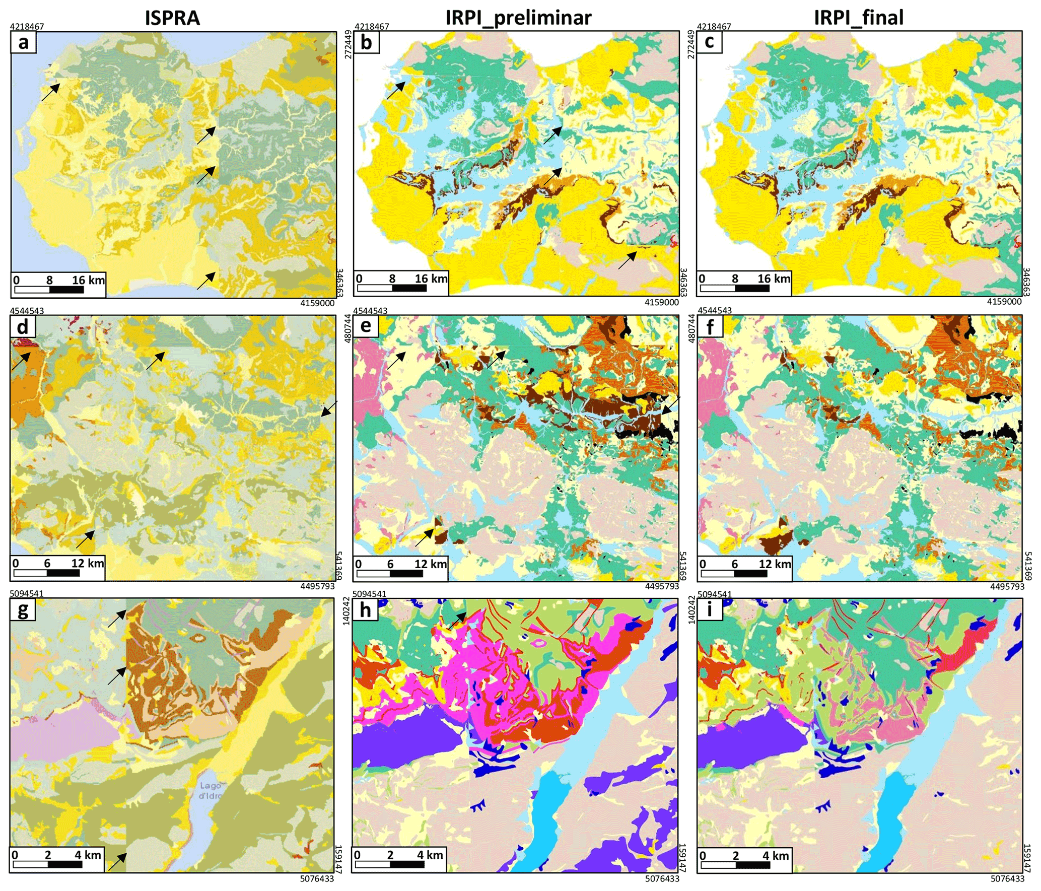
Figure 7 Comparison of two different classifications of the same source dataset for selected areas of the Sicily (a, b, c), Campania (d, e, f), and Lombardy (g, h, i) regions. Examples from the lithological map of Italy according to the ISPRA classification as visualized in vector form at the ISPRA website (Table 1, ID 5) are shown in panels (a), (d), and (g). For the same areas, the lithological map of Italy according to our own preliminary semi-automatic classification partially resolved the major inconsistencies along the boundaries of the geological sheets already present in panels (a), (d), and (g), even if critical boundaries still remain; see the black arrows as a reference. Most of the inconsistencies were resolved manually by expert analysis in the final version of our map (c, f, i), leading to a substantial improvement of the lithological harmonization along the borders of the original geological sheets.

6 Data availability

The digital lithological map of Italy at 1:100 000 is provided in the PANGAEA database. It is publicly available at the following web address: https://doi.org/10.1594/PANGAEA.935673 (Bucci et al., 2021).

7 Conclusions

This paper described the first freely downloadable lithological map of Italy at the 1:100 000 scale, providing the distribution of rock attributes and rock types of the Italian territory in digital format.

The LMI was assembled from 277 sheets of the geological map of Italy at the 1:100 000 scale and distributed in digital vector format through a REST service on the ISPRA website. For this purpose, the rock types associated with the ​​​​​​​5456 unique geological descriptions in the source dataset were identified and translated into the 19 general classes defined here. Adjacent polygons grouped within the same class were dissolved, reducing their number from the original 292 705 to the 180 503 in the final product. Most of the work consisted of database queries coupled with expert analysis of the location of the polygons using the sheets available at the 1:50 000 scale (where present) and with any potentially useful information sought in the regional and local literature. Particular attention was paid to harmonizing the lithological information at the boundaries of the original geological sheets. A final technical validation allowed us to detect and resolve residual problems also related to inconsistencies inherited from the source dataset and guaranteed the overall quality of the work.

The LMI allows the assessment of national-scale research questions at high resolution and thus helps to advance our knowledge about the relationships between lithology and surface processes, including multiple geomorphological, geohydrological, and environmental issues. In addition, the resolution of the LMI highlights the differences in the lithological cover of the different regions and sub-regions, hence facilitating the comparison of results of different regional studies (e.g. susceptibility to landslides and floods).

The map has limits and can be enhanced, in particular in local areas where geolithological descriptions in the source dataset were not exhaustive and our knowledge is limited. Inclusion of more detailed regional maps or other relevant additional information, e.g. age, tectonic history, geotechnical properties, or fine–coarse grain size ratio, is beyond the aim of this work but may be included in future versions. Aware of these and other potential and desirable future upgrades, we provided the LMI with a very simple and open architecture, which allows more details or levels of information to be added and could thus be developed further in accordance with specific scientific questions.

Appendix A: Data acquisition procedure

ISPRA exhibits a REST service for the publication of spatial data (Table 1, ID 9). The acronym REST stands for “representational state transfer”, which is an architectural style for developing services using the http data transfer protocol. In particular, ISPRA uses the ArcGIS REST API, the Advanced Programming Interface REST developed by ESRI through the proprietary ArcGIS Online platform. The ESRI API can be queried through specific http requests (for example the GET type, in which the service address is followed by a series of key-value information) that allow us, for example, to obtain the representation in JSON (JavaScript Object Notation) format of geometries (geospatial-layer features) and associated attributes. Normally this service is limited to the return of a maximum number of features for each request. The acquisition of the database required (i) knowledge of the REST service APIs and (ii) a procedure for the automatic download of subsets of data, which cannot be downloaded in a single piece by the design of the website, and (iii) merging of all of the subsets into a single vector map. To execute the download, we prepared a script to download subsets of 100 polygons (geometric features) for each single call to the service, using the Linux wget command. The procedure is simple and consists of a loop in which, at each iteration, a number (Δ) of polygons (100 in the actual case) out of the 300 000 total available polygons. Given that the API of the REST service database was unknown to us, we followed a trial-and-error procedure to obtain a working script. Downloaded data consisted of 2927 files in GeoJSON format, which we converted to a single ESRI shapefile using the GDAL/OGR library.