One hundred plus years of recomputed surface wave magnitude of shallow global earthquakes

Among the multitude of magnitude scales developed to measure the size of an earthquake, the surface wave magnitude M_s is the only magnitude type that can be computed since the dawn of modern observational seismology (beginning of the 20th century) for most shallow earthquakes worldwide. This is possible thanks to the work of station operators, analysts and researchers that performed measurements of surface wave amplitudes and periods on analogue instruments well before the development of recent digital seismological practice. As a result of a monumental undertaking to digitize such pre-1971 measurements from printed bulletins and integrate them in parametric data form into the database of the International Seismological Centre (ISC, http://www.isc.ac.uk, last access: August 2021), we are able to recompute M_s using a large set of stations and obtain it for the first time for several hundred earthquakes. We summarize the work started at the ISC in 2010 which aims to provide the seismological and broader geoscience community with a revised M_s dataset (i.e., catalogue as well as the underlying station data) starting from December 1904 up to the last complete year reviewed by the ISC (currently 2018). This M_s dataset is available at the ISC Dataset Repository at https://doi.org/10.31905/0N4HOS2D (International Seismological Centre, 2021d).

1 Introduction

Since its introduction, the surface wave magnitude M_s has been very popular, and for a long period of time, before the moment magnitude M_w was introduced by Kanamori (1977) and Hanks and Kanamori (1979), it was considered the most reliable magnitude to estimate an earthquake size. Its popularity originated due to the following: (a) as opposed to the magnitude concept introduced at a local scale by Richter (1935), M_s allows seismologists to compute magnitudes for earthquakes worldwide, including those recorded at teleseismic distances (i.e., from 20^∘ onward), without relying on local recordings that were not available in most seismic zones; (b) thanks to the work of station operators, analysts and researchers at various observatories around the world that produced readings of surface wave data for shallow earthquakes since the beginning of the last century, M_s can be computed (systematically) since the dawn of instrumental seismology (Fig. 1). In addition, M_s is probably the only type of earthquake magnitude that can be computed systematically for all damaging earthquakes for the last 100+ years. However, as any magnitude type M_s also has shortcomings, such as the possible underestimation for some large earthquake (as discussed later), the inability of processing surface waves from short-period instruments (hence for many small local earthquakes) and the limitation, at least in standard procedures (IASPEI, 2013), of being defined for shallow earthquakes.

Figure 1 Availability over time of common magnitude scales for worldwide (M_s, M_w, broad-band and short-period body-wave magnitude m_B and m_b, respectively) and local/regional (e.g., Richter and duration magnitude M_l and M_d, respectively) earthquakes. Solid thick black lines represent time periods over which a magnitude scale is available or can be recomputed systematically (dashed–dotted thin grey lines otherwise). For local/regional magnitudes the availability only regards limited continental areas (Di Giacomo and Storchak, 2016). Listed on top are some significant developments in terms of earthquake magnitude. Among those GTT refers one of the first printed station bulletins produced at the Göettingen observatory in Germany (Schering, 1905), which pioneered modern observational seismological practice, and GCMT is the Global Centroid Moment Tensor project (https://www.globalcmt.org, last access: August 2021, Dziewonski et al., 1981; Ekström et al., 2012).

Gutenberg (1945), using measurements of amplitudes and periods of surface waves accumulated during the first 40 years of the last century, introduced M_s as

$$M_{\mathrm{s}}=\log A+\mathrm{1.656}\log \mathrm{\Delta }+\mathrm{1.8}.$$

Since then a team of researchers from Moscow and Prague further developed Gutenberg's work and proposed the formula (Kárník et al., 1962; Vanĕk et al., 1962)

$$M_{\mathrm{s}}=\log {\left({\displaystyle \frac{A}{T}}\right)}_{max}+{\mathit{\sigma }}_S\left(\mathrm{\Delta }\right)=\log {\left({\displaystyle \frac{A}{T}}\right)}_{max}+\mathrm{1.66}\log \mathrm{\Delta }+\mathrm{3.3},$$

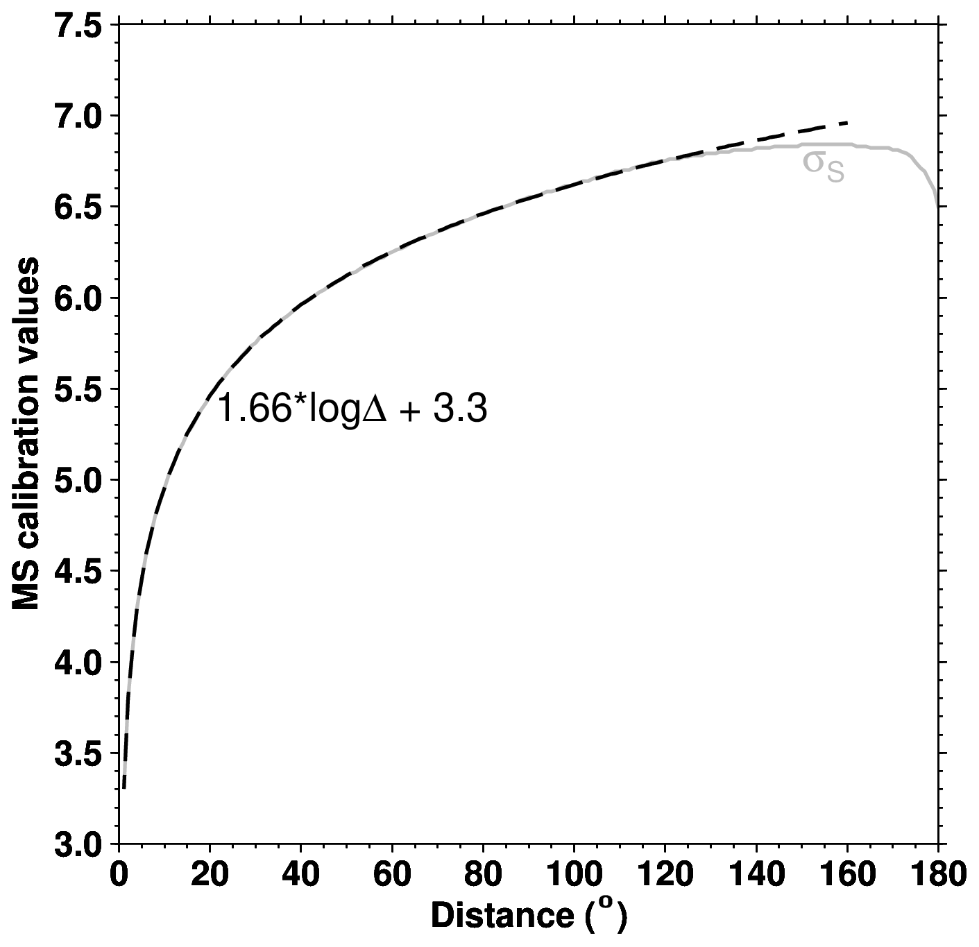
where A and T are the amplitude (in µm) and period (in s) of the surface wave train, respectively, and Δ is the distance in degrees of the seismic station from the earthquake epicentre (distance and period limits will be discussed in the next section). This is the so-called Moscow–Prague formula, and it was accepted as the standard for M_s computation by the International Association of Seismology and Physics of the Earth's Interior (IASPEI, http://www.iaspei.org/, last access: August 2021) at the 1967 Zurich meeting (Bormann et al., 2012; IASPEI, 2013). The calibration function σ_S(Δ) and its best fit up to 160^∘ (1.66log Δ+3.3) are shown in Fig. 2.

Figure 2 M_s calibration function (tabulated values, σ_S) from the Moscow–Prague (grey solid curve) group and its best fit for distances between 2 and 160^∘ (1.66log Δ+3.3, black dashed curve). See Bormann (2012) for details.

Several earthquake catalogues that listed M_s have served the seismological community for various purposes in the past decades. One that has been instrumental for many studies is Abe's catalogue (Abe, 1981; Abe and Noguchi, 1983a, b; Abe, 1984). This catalogue lists M_s values for large earthquakes (mostly M_s>6.5) up to 1980, and its reliability was recently confirmed by Di Giacomo et al. (2015a). Since then researchers have extend Abe's catalogue beyond 1980 with M_s solutions from the International Seismological Centre (ISC, http://www.isc.ac.uk, last access: August 2021) and/or the National Earthquake Information Center of the USGS (https://earthquake.usgs.gov/earthquakes/search/, last access: August 2021). Such a composite M_s catalogue was then used as the magnitude basis for recent compilations such as the Centennial Catalogue (Engdahl and Villaseñor, 2002) and PAGER-CAT (Allen et al., 2009) as well as various types of research, from calibration purposes (Herak and Herak, 1993; Rezapour and Pearce, 1998) to patterns of the Earth's seismicity (e.g., Pérez and Scholz, 1984; Ogata and Abe, 1991; Pacheco and Sykes, 1992; Pérez, 1999).

Considering the important legacy of M_s in the seismological community, here we present a revised M_s catalogue (cut-off magnitude of 4.5) listing over 46 000 earthquakes as well as the underlying station data (files described in Sect. 7) used to derive M_s for each earthquake. Hereafter we refer to the catalogue and underlying station data as the ISC M_s dataset (International Seismological Centre, 2021d). To create this product we benefit from the work done by Di Giacomo et al. (2015b, 2018) to digitize (i.e., converted from printed to computer accessible format) a large volume of surface wave parametric data prior to 1971 and by Storchak et al. (2017, 2020) to rebuild the ISC Bulletin from 1964 onwards.

We first recall the basic steps in our procedure to compute M_s and outline the major features of the station data behind the calculation of the network M_s. Then we discuss some properties of the ISC M_s dataset in terms of completeness and rates in different time periods. Finally, we briefly discuss the largest earthquakes ever recorded and outline further activities that could improve this dataset in different time periods.

2 Reporters and M_s recomputation

A big part of the ISC mission consists of collecting and reprocessing reports from seismological agencies all over the world to produce the ISC Bulletin (International Seismological Centre, 2021c). Details about agencies contributing data to the ISC can be found at http://www.isc.ac.uk/iscbulletin//agencies/ (last access: August 2021). The summary of the agencies (hereafter also referred to as reporters or data contributors) that contributed surface wave parametric data to create the ISC M_s dataset is shown in Fig. 3. A few aspects are worth mentioning regarding the surface wave data reporters.

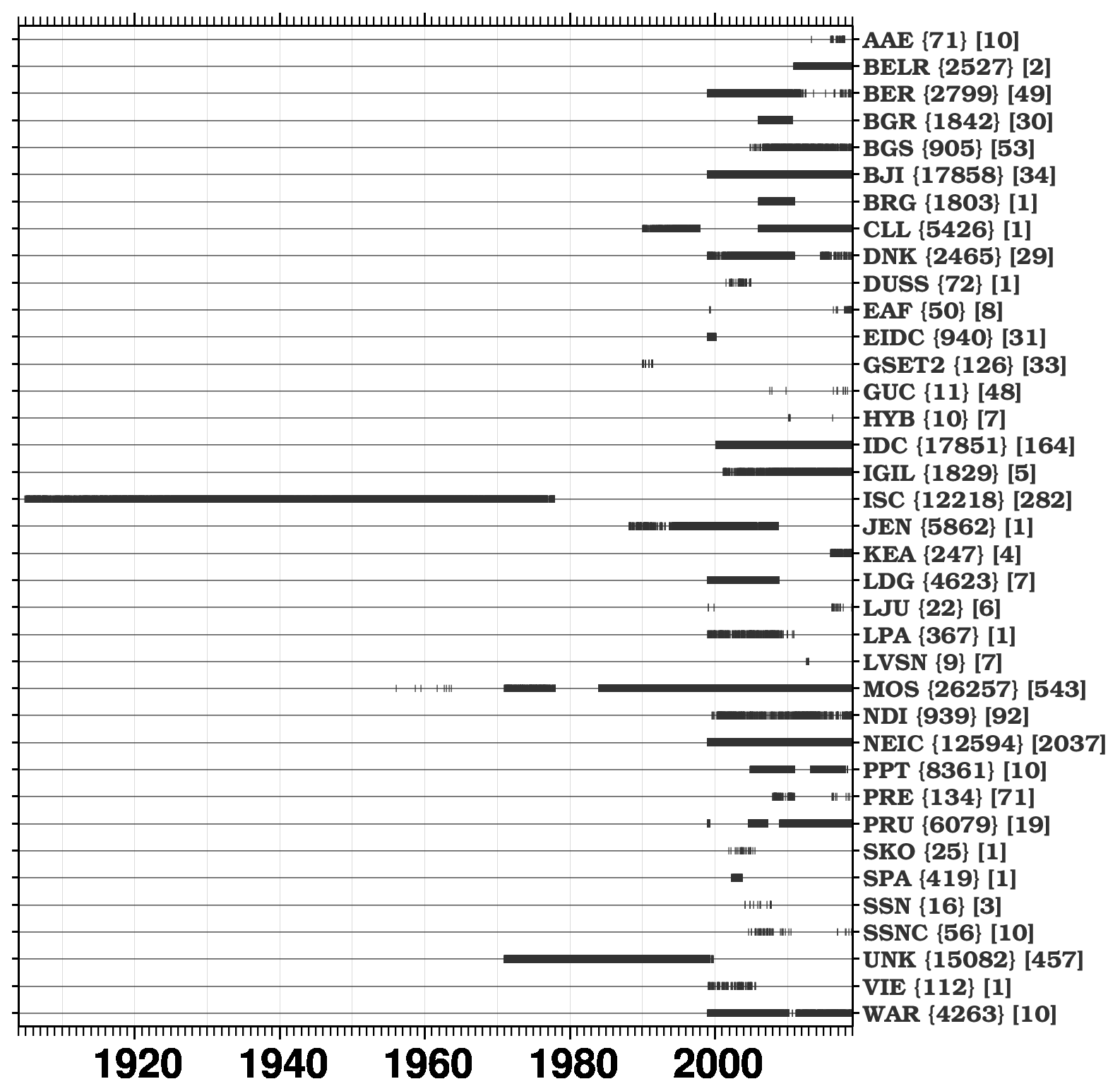
Figure 3 Timelines of the agencies contributing with surface wave data (amplitude and period measurements). Each symbol represents the origin time of an earthquake. Details about each agency code can be found by typing the agency code at http://www.isc.ac.uk/iscbulletin//agencies/ (last access: August 2021). The total number of earthquakes and stations for each agency are listed in curly and square brackets, respectively. Note that a reporter that is UNK (unknown) is not a genuine reporter code, but it simply represents data collected before the ISC database was set up, i.e., when the association between data and reporter was not maintained.

Originally, the ISC had no surface wave data available in digital form for pre-1971 earthquakes. Hence, to fill this data gap, an onerous undertaking of digitizing surface wave data from station/network printed bulletins began in 2010 (Di Giacomo et al., 2015b, 2018). As shown in Fig. 3, this effort resulted in the ISC having digitized surface wave data from a total of 282 stations for over 12 000 earthquakes (it is our intention to continue this effort; see Sect. 6).

Between 1971 and 1998 the ISC Bulletin contains surface wave data from 457 stations worldwide. However, in this time period we cannot associate such data to specific reporters (hence reporter is UNK, unknown, in Fig. 3). The only exceptions to that are data reports (e.g., agency MOS, JEN, CLL) parsed in the ISC Bulletin during the Rebuild project (Storchak et al., 2017, 2020). Since 1999, coinciding with a major update in ISC data collection procedures and the setup of the ISC database, we are able to routinely associate station data with their agency. Only 30 reporters out of about 150 contributed surface wave data in the last 20 years, with the largest contributors being IDC, NEIC, MOS and BJI (Fig. 3).

Our approach to computing M_s closely follows the standard ISC procedure (Bondár and Storchak, 2011) and is already detailed in Di Giacomo et al. (2015a). However, it is beneficial here to (1) recall some aspects of the procedure in light of the content of station data files (Sect. 7) and (2) explain some necessary deviations from it.

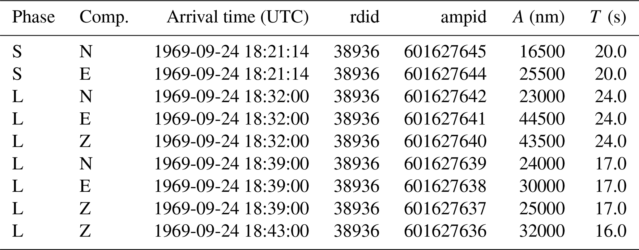
First, we consider the surface wave data belonging to a reading (in ISC jargon a reading groups all parametric data from a single station associated to a specific seismic event and reported by the same agency). A reading can have any number of surface wave data entries, and different reporters may provide a reading for the same station. An example of a reading is shown in Table 1 for station CLL (Collm, Germany) for an earthquake which occurred in the northern Mid-Atlantic Ridge, 24 September 1969. We have chosen this example as the reading lists multiple surface wave data entries on all three components. Within the surface wave phases of the reading (L in our example), we first search for the maximum of $\frac{A}{T}$ on the vertical component, and, if available, the component magnitude M_sZ is obtained via the Moscow–Prague formula. Then, for periods within ±10 s of T on the vertical component, the maximum of $\frac{A}{T}$ for the horizontal vector component

$$\sqrt{{\left({\displaystyle \frac{A}{T}}\right)}_N^{\mathrm{2}}+{\left({\displaystyle \frac{A}{T}}\right)}_E^{\mathrm{2}}}$$

is searched to calculate the component M_sH magnitude. If one of the two horizontal components is not available then

$${\left({\displaystyle \frac{A}{T}}\right)}_{\mathrm{H}}=\sqrt{\mathrm{2}\cdot {\left({\displaystyle \frac{A}{T}}\right)}_{N|E}^{\mathrm{2}}}.$$

Although our procedure finds the maximum of $\frac{A}{T}$ within the reading, a reporter may have provided single component measurements of $\frac{Amax}{T}$. In our CLL reading example the maximum $\frac{A}{T}$ on the vertical component is defined by ampid equal to 601627636, whereas ampid equal to 601627639 and 601627638 on the north–south and east–west component, respectively, defines the maximum horizontal vector component. Such defining entries are included in the station data files (more details in International Seismological Centre, 2021d). Then the M_s for the reading is computed as $(M_{\mathrm{s}Z}+M_{\mathrm{sH}})/\mathrm{2}$ if both exists, or $M_{\mathrm{s}}=M_{\mathrm{s}Z|\mathrm{H}}$ if one of them is not available. If more than one reading M_s exists for a station, the median of the readings M_s is used as station M_s. Finally, the network M_s is computed as the median of the stations M_s if at least three or five station magnitudes are available prior to or since 1971, respectively. The uncertainty of the network M_s is expressed as the standard median absolute deviation (SMAD) of the α-trimmed station magnitudes (α=20 %).

Table 1 Reading example from station CLL (Collm, Germany) associated to an event in the northern Mid-Atlantic Ridge that occurred on 24 September 1969 ($\mathrm{\Delta }=\mathrm{58.8}{}^{\circ }$). The surface wave measurements (L phases) are used by our procedure to obtain the reading M_s. The database identifiers for the reading and single amplitude-period entries, respectively, are rdid and ampid. See text for details.

In line with IASPEI recommendations (IASPEI, 2013), we only allow M_s for earthquakes with depth ≤ 60 km. The locations adopted in this work come from the ISC-GEM Catalogue (Bondár et al., 2015; Di Giacomo et al., 2018) between 1904 and 1963 and the rebuilt ISC Bulletin (Storchak et al., 2017, 2020) from 1964 onward.

Standard procedures at the ISC consider surface wave periods between 10 and 60 s and distances between 20 and 160^∘. Such delta-period ranges are also adopted here for earthquakes which occurred after 1963 (hereafter also referred to as standard delta-period ranges). Prior to 1964 we expand the period and distance ranges to 5–60 s and 2–180^∘, respectively, as discussed in Di Giacomo et al. (2015b). The augmentation of the delta-period limits prior to 1964 is mainly due to the relative scarcity of surface wave data in the first part of the last century compared to its second half (hence the need for not discarding station M_s) and to changes in seismological practice in many institutes coinciding with the introduction of the World-Wide Standardized Seismograph Network (WWSSN, Oliver and Murphy, 1971; Peterson and Hutt, 2014). When stations beyond 160^∘ are used we use the tabulated values of σ_S(Δ) instead of its best fit (Fig. 2), as recommended by Bormann et al. (2012). In the next section we show that the amplitude/period measurements prior to the WWSSN introduction justify our delta-period expansion for pre-1964 earthquakes.

3 Station data

The decadal spatial distribution of the stations contributing to the ISC M_s dataset is summarized in Figs. 4–5. At times we mention seismic stations that, for sake of brevity, we may only identify by their code (station's full details can be accessed at International Seismological Centre, 2021b).

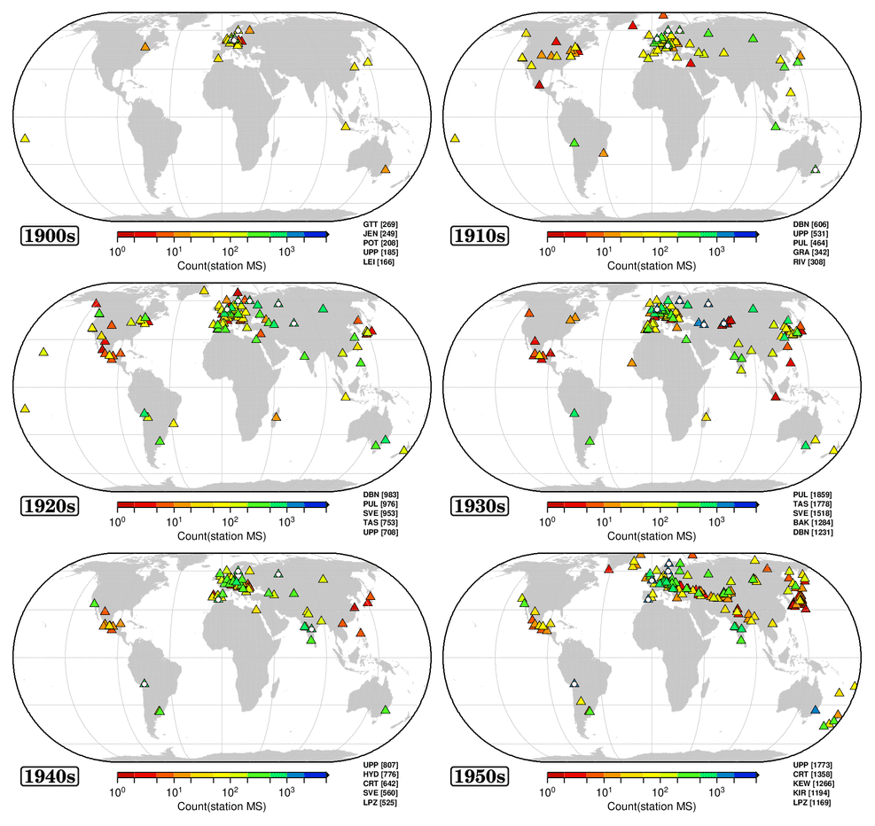
Figure 4 Decadal (up to the 1950s) distribution of the stations (triangles) that contributed with surface wave data. Symbols are colour-coded by number of station M_s. For each decade, the top five stations in terms of Count(station M_s) are identified by a white circle and listed in the bottom-right corner outside each map. Maps drawn using the Generic Mapping Tools (GMT) (Wessel et al., 2013) software. Plots of the annual station M_s distributions are included in International Seismological Centre (2021d).

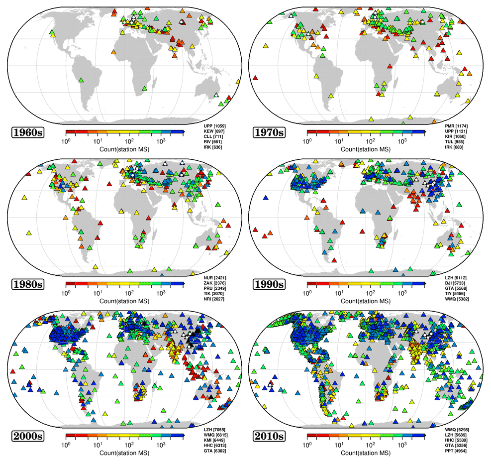
Figure 5 As for Fig. 4 but since the 1960s. Maps drawn using the Generic Mapping Tools (GMT) (Wessel et al., 2013) software.

Not surprisingly, the M_s network geometry is unbalanced as the Northern Hemisphere features many more stations than the Southern Hemisphere (a known issue in every aspect of instrumental seismology). In more detail, these figures highlight how the M_s network became more dense and widespread over time after most of the stations were located in Europe at the beginning of the last century. Indeed, most of the M_s measurements in the first two decades of the last century heavily rely on stations in Germany (e.g., GTT, JEN), UPP in Sweden and a few others (e.g., DBN in the Netherlands and PUL in Russia). From the 1920s to the 1960s the station density increased in Europe and in former Soviet Union territory. North American stations also contributed but for a small number of earthquakes.

The Southern Hemisphere had only a handful of M_s reporting stations up to the 1970s–1980s. However, thanks to the extraordinary efficiency in observatory practice at the Observatorio San Calixto (LPZ, Bolivia, opened in 1913, Coenraads, 1993) and Riverview (RIV, Australia, opened in 1909, Drake, 1993), both from the Jesuit network (Udias and Stauder, 1996), our capabilities of obtaining M_s improved significantly in the first half of last century both for Southern Hemisphere and worldwide earthquakes, as was noted by Gutenberg and Richter (1954).

From the 1970s, when surface wave data started to be digitally available in the ISC Bulletin, we witness a significant increase in the M_s network coverage, particularly in the last two decades, where many more stations in the Southern Hemisphere have contributed to M_s. However, their spatial distribution is not yet as dense as in North America or the Euro-Mediterranean area.

To summarize the evolution of the M_s network over the decades, Fig. 6 shows the network M_s decadal box-and-whisker plot of the number of stations (N_sta) and secondary gap (i.e., the largest azimuthal gap in which only one station exists, and the quality of the data at that station may bias the solution). The latter parameter is normally used as a network geometry parameter in earthquake location (Bondár et al., 2004), but here it is used as a measure of the azimuthal coverage of the station contributing to M_s computation (both gap and secondary gap are included in the M_s catalogue file). Ideally, the station distribution should sample the focal sphere from different azimuth to reduce the effects of propagation path heterogeneities and radiation pattern (von Seggern, 1970) on the network M_s, although the latter is symmetric for surface waves (either two-lobed or four-lobed). In light of the station distributions shown in Figs. 4–5, it is not surprising that for most of the last century the secondary gap is usually 180–270^∘ or above, meaning that the stations contributing to the network M_s are often located in a narrow azimuth. To showcase the possible effects of this aspect, in Fig. A1 we show the azimuthal distribution of the station M_s for the 20 March 1960 earthquake off the east coast of Honshu (event 878564). Most of the M_s stations are located in Europe, and it appears that those are responsible for making the network M_s=7.9, as most of the station magnitudes at different azimuth are well below the final network M_s. Nevertheless, significant improvements in the station azimuthal coverage occur from the 1970s, and with the increase in N_sta we observe an overall decrease in secondary gap.

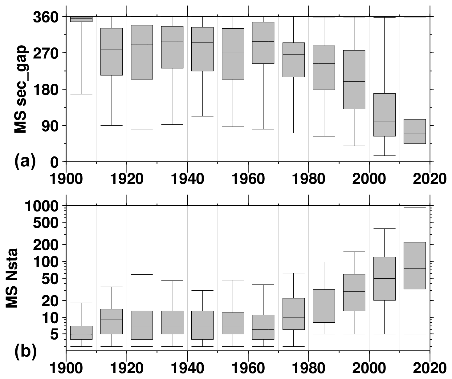
Figure 6 Decadal box-and-whisker plot of the secondary gap for M_s (a) and number of M_s stations (b).

The final aspect of the station data we discuss here regards the period at which the amplitudes of the surface waves are measured. We do that by showing, similarly to Bormann et al. (2009, 2012), the distance-period distributions of $(\frac{A}{T}{)}_{max}$ for earthquakes prior to and since 1964 (Fig. 7 and Fig. 8, respectively). The separation in these two time periods is linked both to the start of the original ISC Bulletin (Adams et al., 1982) in 1964 and a change in observatory practice by many institutions due to the WWSSN introduction in the early 1960s. The standard WWSSN practice produces amplitudes of surface waves as measured for T around 20 s (usually ±2 or ±3 s) for distances ≥ 20^∘ (in addition, measurements on the vertical component were preferred to horizontal ones since the 1970s). Before WWSSN, however, the standard practice was to measure the surface wave amplitudes in broader period ranges (such differences led IASPEI, 2013, to recommend the computation of two types of M_s, M_s20 and M_sBB). Therefore, before 1964 we observe in Fig. 7 that T falls reasonably well within the expected period ranges of Vanĕk et al. (1962) (i.e., amplitudes measured over a broad T range and using data below 20^∘), whereas from 1964 onward we see surface amplitudes predominantly measured around T of 20 s throughout the entire distance range, as shown by the vertical component of Fig. 8. The surface wave amplitude-period measurements pre-WWSSN, therefore, allow us to expand the delta-period limits for pre-1964 earthquakes as outlined in Sect. 2.

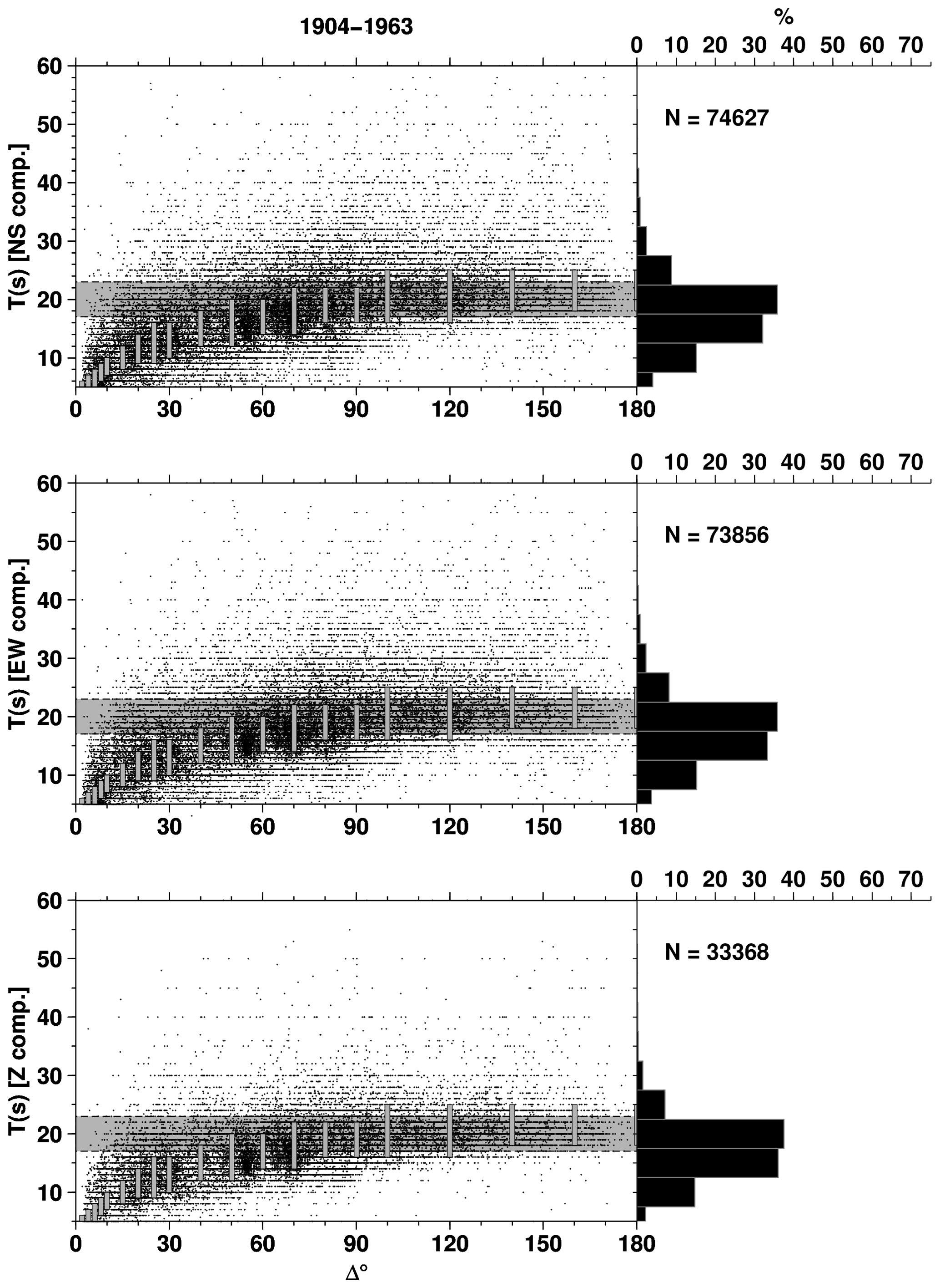
Figure 7 Three-component distance-period plots of $(\frac{A}{T}{)}_{max}$ for surface wave readings digitized from printed bulletins for earthquakes that occurred before 1964. The horizontal grey shaded area depicts measurements around 20 s, whereas the vertical grey bars represent the expected period ranges at various distances (Vanĕk et al., 1962) as published in Table 3.2.2.1 of Willmore (1979). The histograms on the right-hand side show the period distribution in bins of 5 s. See text for details.

Figure 8 As for Fig. 7 but for 1964–2018.

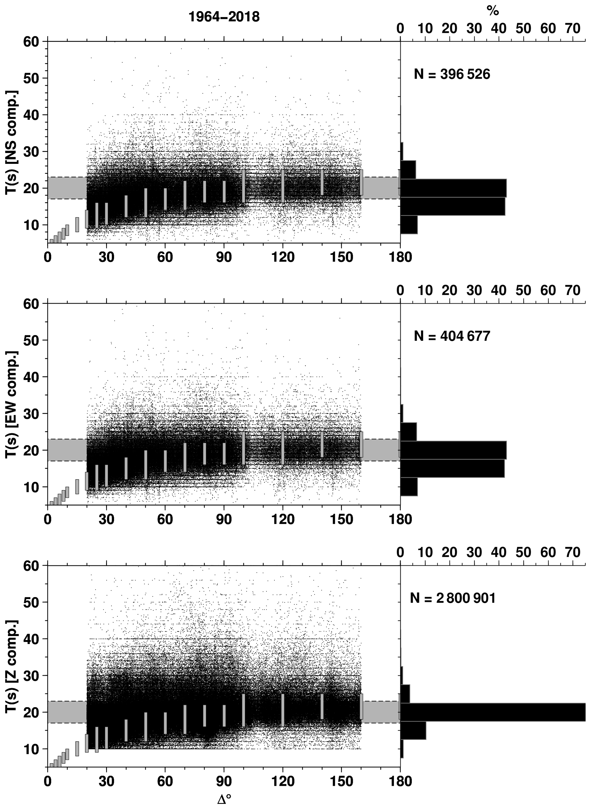
However, not all reporters fully adopted WWSSN standards. Indeed, among the largest ones (Fig. 3), agency BJI, MOS and PRU report surface wave amplitudes in broad period ranges. The delta-period plots of those agencies are shown in Appendix A (Figs. A2, A3 and A4). Other agencies, instead, strictly adhere to amplitude-period measurements around 20 s (Figs. A5, A6 and A7, for agencies IDC, LDG and NEIC from 2009, respectively).

As a final remark in this section, we reiterate, as already done in Di Giacomo et al. (2015a), that the differences in distance and period ranges do not introduce a discontinuity in the M_s estimates before and after 1964. The expansion of the delta-period limits pre-1964 is allowed by the data, and it often gives us the opportunity to increase N_sta for our network M_s computation in a time period where surface wave data were scant (compared to current times) and not digitally available (hence the need of not discarding precious and hard-to-get data). As a result of our approach, about 40 % of the pre-1964 earthquakes we list in the ISC M_s dataset gained from 1 to 28 station magnitudes, and 1000 of those earthquakes would not have network M_s without delta-period augmentation. This is synthesized in Fig. 9. An area encompassing the North Atlantic mid-oceanic ridges, the Euro-Mediterranean and the Middle East benefitted the most thanks to European and central Asian stations that measured surface waves in broad period ranges at distances below 20^∘.

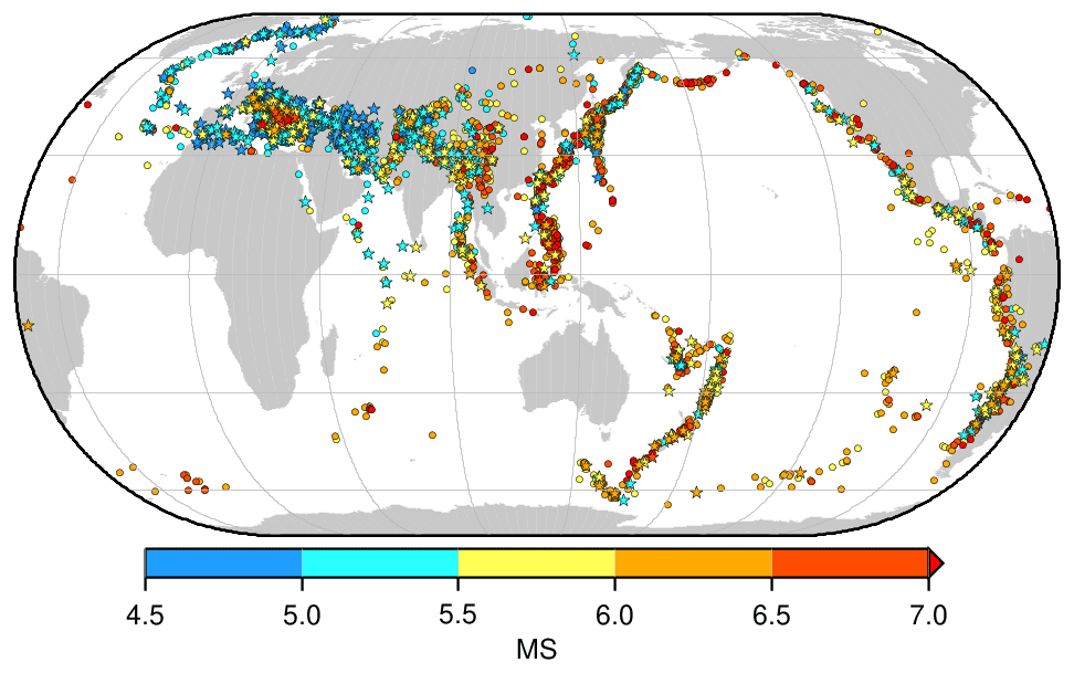
Figure 9 Map of the pre-1964 earthquakes where the expansion of the delta-period ranges compared to the current ISC practice allowed us to better constrain M_s. Stars are for the 1000 earthquakes that otherwise would not have network M_s. All symbols colour-coded by M_s. Map drawn using the Generic Mapping Tools (GMT) (Wessel et al., 2013) software.

4 Catalogue properties

The ISC M_s dataset has a minimum cut-off magnitude of 4.5. Earthquakes with lower M_s values are available in the ISC Bulletin but mostly in recent decades. The major improvements regard earthquakes prior to 1964, where, according to our records, out of 10 057 earthquakes the ISC is the first to compute M_s for 4940 of them (their distribution and timeline is shown in Fig. A8). Considering the whole ISC M_s dataset, major features can be discussed using Fig. 10, where we show the magnitude timeline, number of earthquakes per year for various magnitude thresholds and annual magnitude of completeness (M_c) computed with the maximum curvature method of Wiemer and Wyss (2000). The completeness analysis is only meant to highlight general features of the dataset (a more detailed study in this respect, as the one by Michael, 2014, is not the aim of this work). As in any other earthquake catalogue, we cannot include all shallow earthquakes since some of them may be poorly recorded or not matching our selection criteria. Hence, we perform annual M_c estimations knowing that the dataset may have missing records. This is more likely to be the case in the first part of the last century. As a result, annual M_c uncertainties (error bars in the top panel of Fig. 10) are generally larger for the early decades of the last century compared to recent times.

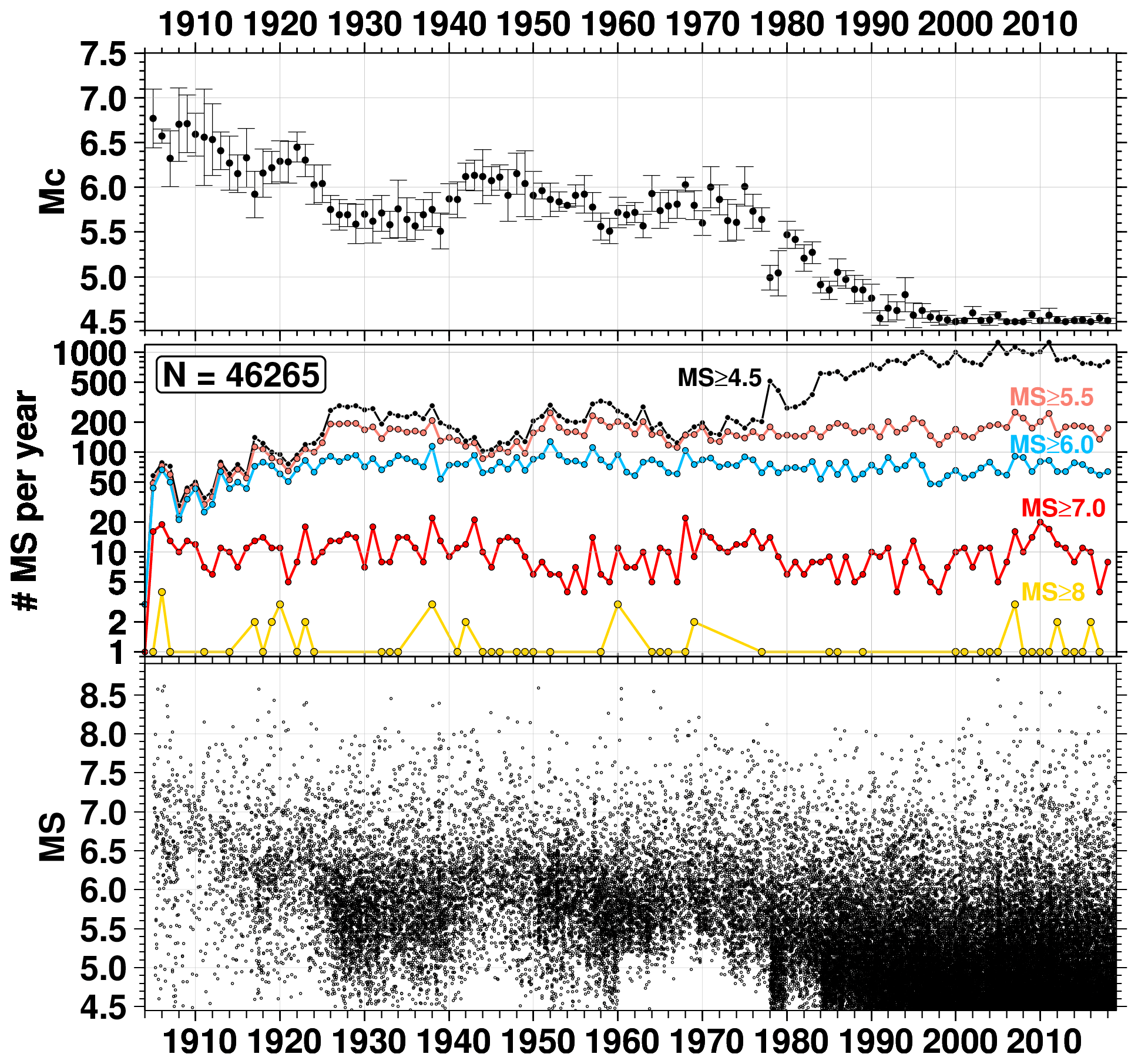
Figure 10 Bottom panel: magnitude timeline of the ISC M_s dataset. Middle panel: number of M_s per year for different M_s thresholds (4.5, 5.5, 6.0, 7.0 and 8.0 in black, light red, blue, red and yellow, respectively). Top panel: annual magnitude of completeness M_c (Wiemer and Wyss, 2000) in the dataset, shown as average ±1 standard deviation.

Overall, we include M_s<5.5 earthquakes mostly from the 1980s, and M_c approaches approximately 4.5 in the last 20 years. We note that we were able to obtain more solutions at the low magnitude end particularly in the late-1920s–1930s. This has been possible thanks to the establishment of the backbone network in former Soviet Union territory and a general increase of M_s stations in other areas (see annual station maps in International Seismological Centre, 2021d). An overall dip is observed in the 1940s, most likely caused by the disruption of World War II on the seismic network (Di Giacomo et al., 2018). The period 1960–1977 also features fewer earthquakes below 5.5 than the previous and following decades. This is due both to the limited number of stations available and the fact that we digitized surface wave data from the 1960s printed station bulletins only for earthquakes selected in the first version of the ISC-GEM Catalogue (magnitude 5.5 and above, Storchak et al., 2013). In Sect. 6 we propose activities that are likely to mitigate significantly the deficiencies of the ISC M_s dataset in most of the 1960s–1970s. Another fluctuation at low magnitudes is observed in the early-1980s. Indeed both the annual counts and M_c show a significant variation from 1978–1979 (M_c close to 5.0) to 1980–1983 (higher M_c ranging between 5.2–5.5). We believe this is due to the temporary absence of MOS surface wave data in 1980–1983 (see Sect. 6), which was included into the rebuilt ISC Bulletin (Storchak et al., 2020) from 1984 onward (M_c dropping again to about 5 and below).

Weaker variations are seen for moderate size earthquakes (i.e., M_s between 5.0 and 6.0). The early part of last century (up to the mid-1920s) is clearly complete above magnitude 6.0, whereas since the 1950s the frequency of M_s 5.5 and 6.0 appears rather stable. Pronounced variations are observed from the mid-1920s to the 1940s for reasons mentioned above.

Variations over time of the frequency of large (i.e., M_s≥6.0) earthquakes based on past catalogues have been the subject of debate in past literature. In particular, Pérez and Scholz (1984) suggested that, under the assumption of constant rate earthquake occurrence, temporal variations of large shallow earthquakes were driven by instrumental changes. Ogata and Abe (1991) and more recently Ogata (2021), however, suggest that variations in the frequency of global large earthquakes are a real effect of the Earth's seismic activity (long-range dependence nature of earthquake occurrence). Therefore, to further discuss the rate of the Earth's large shallow seismicity, we show in Fig. 11 the cumulative number of strong to major earthquakes in the ISC M_s dataset similarly to the figures in Pérez and Scholz (1984) and Pérez (1999). Compared to these works, our rates for M_s ≥ 7.0 and 6.0 in different time intervals (Table 2) show some significant differences and lack large jumps from one period to another. This is strikingly evident for the M_s ≥ 6.0 distribution, where the Pérez (1999) rate goes down to 38 yr⁻¹ during 1964–1978 compared to a rate of about 78 yr⁻¹ in the ISC M_s dataset. We note that this period in the original ISC Bulletin lacked the ISC's own computations of M_s. Therefore, Pérez (1999) rates may have been biased by using largely incomplete inputs.

(Pérez and Scholz, 1984)(Pérez, 1999)

Table 2 Rates of seismicity in the ISC M_s dataset and in Pérez and Scholz (1984); Pérez (1999). See text for details.

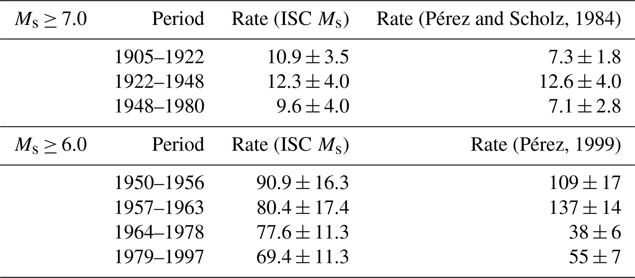
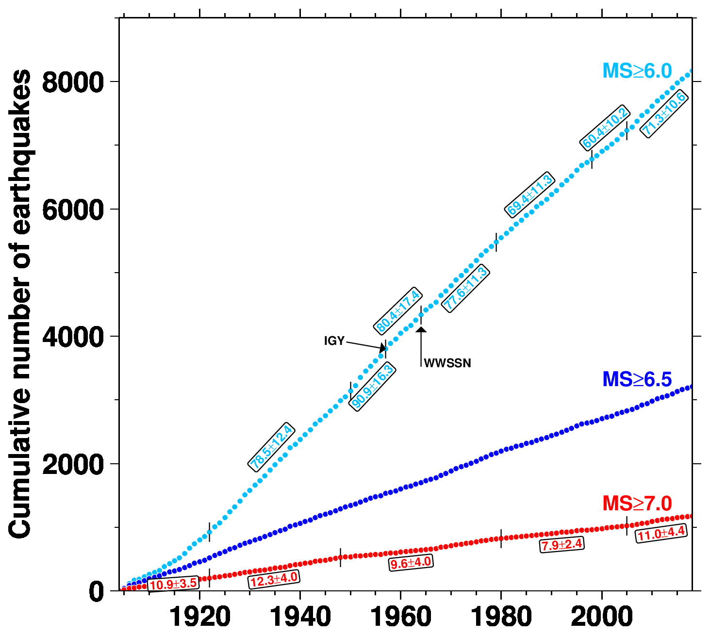
Figure 11 Cumulative number of earthquakes with M_s ≥ 7.0 (red), ≥ 6.5 (blue) and ≥6.0 (cyan). The vertical black segments on the red and cyan symbols locate the time periods considered by Pérez and Scholz (1984) for M_s ≥ 7.0 (up to 1980) and Pérez (1999) M_s ≥ 6.0 (from 1950 to 1997), respectively. IGY stands for International Geophysical Year started in 1957. See text for details.

In general, we see that shallow seismicity rates are characterized by a global low occurring between the great earthquakes of the early 1960s and the beginning of the current century (Ammon et al., 2010). Although rates for M_s ≥ 7.0 in the first part of the last century are comparable to the rate we have observed since 2005, it seems that rates for M_s ≥ 6.0 from the WWSSN introduction appear to be lower than rates in the first part of the last century. We also assessed if by declustering (Reasenberg, 1985) the M_s catalogue the rates would be different but only small variations occur, and, more importantly, relative differences between time periods remain. This is not surprising as the ISC M_s dataset does not contain a large number of aftershocks for M_s ≥ 6.0 (by the very nature of M_s it is more difficult to obtain it for aftershocks of large earthquakes due to association challenges in overlapping signals, particularly in routine operations).

It is not the aim of this work to investigate whether fluctuations in seismic activity rates are partially due to instrumental changes or purely due to natural variations of the Earth's seismicity. However, we believe that the ISC M_s dataset is one of the best inputs to date to do such studies. In this context it is important to point out that the quality of instrumental earthquake catalogues depends on the quality of the data available at the time of processing. In our experience, for long-term datasets it is almost unavoidable that different types of shortcomings may occur in different time periods, for example due to external factors (e.g., network deficiencies during world wars) and that faulty individual entries may be present. It is of paramount importance, therefore, that datasets are well documented and that users know how they are created in order to properly use them for research.

5 On the M_s saturation and large differences with M_w

By the time M_s was introduced by Gutenberg (1945), no magnitude 9 or 9+ earthquake had been recorded instrumentally. The occurrence of the 4 November 1952 Kamchatka earthquake and the well-know great earthquakes of the early 1960s (22 May 1960 Chile and 28 March 1964 Alaska earthquakes) drew attention to a shortcoming of M_s, which is commonly referred to as magnitude saturation. This was one of the factors that led Kanamori (1977) and Hanks and Kanamori (1979) to introduce the moment magnitude M_w, which is based on a physical parameter of the seismic source (i.e., seismic moment) rather than amplitude-period measurements.

In Fig. 12 we compare the ISC M_s dataset with M_w from GCMT and the bibliographic search for pre-1976 earthquakes of Lee and Engdahl (2015) and follow-up updates as listed at http://www.isc.ac.uk/iscgem/mw_bibliography.php (last access: August 2021; hereafter referred to as M_w from the literature). Such magnitude comparison has been discussed in several papers, particularly to derive magnitude conversion relationships. For this work, however, we show this comparison to focus on the M_s saturation issue and briefly touch upon earthquakes with large (M_w–M_s) differences.

Figure 12 Comparison of M_s with M_w from GCMT (black dots) and from the literature (red, Lee and Engdahl, 2015, and further updates listed at http://www.isc.ac.uk/iscgem/mw_bibliography.php, last access: August 2021). The black solid curve is a digitized version of the midpoint M_w–M_s curve shown in Fig. 4b of Kanamori (1983). The largest 10 earthquakes in terms of M_w (bulls eye symbols) are also identified by the event code in the ISC Event Bibliography (http://www.isc.ac.uk/event_bibliography/index.php, last access: August 2021).

The 10 largest earthquakes (in M_w terms) ever recorded are easily identified in Fig. 12 by the event code in the ISC Event Bibliography (Di Giacomo et al., 2014; International Seismological Centre, 2021a). As already summarized by Kanamori (1983), the saturation of M_s is generally expected to start between 8.2 and 8.5. For recent (26 December 2004, Sumatra, and 11 March 2011, Tohoku) and pre-GCMT earthquakes (the above-mentioned 1960 Chile and 1964 Alaska earthquakes) with M_w 9 and above, the effects of saturation are quite severe and vary between 0.6 and 1 magnitude unit (m.u.). However, for earthquakes with M_w between 8 and 9, the variation of the saturation appears to vary much more (from near to 0 up to 1 m.u.). For example, the 27 February 2010 M_w 8.8 Maule earthquake has an M_s only 0.25 m.u. smaller, which is close to common M_w–M_s differences observed across a wide magnitude range before the saturation of M_s is expected. Figure 12 shows other examples where M_w and M_s are close to the 1:1 line between 8 and 8.7 (including the 15 August 1950 Assam earthquake). With regard to great earthquakes with large M_w–M_s differences, some of those belong to a peculiar category, the so-called tsunami earthquakes (Kanamori, 1972). These have a relatively small M_s compared to their M_w and are well documented in the literature. The most striking example is probably the 1 April 1946 Aleutian earthquake, where our M_s of 7.4 is much smaller than the M_w 8.6 by López and Okal (2006). On the other hand, large differences are observed for other earthquakes (e.g., 4 February 1965 Rat Islands and 28 March 2005 Nias earthquakes) not strictly considered tsunami earthquakes.

In light of the M_s values for the largest earthquakes ever recorded, we support the remarks by Bormann (2011) that it would be more correct to speak of M_s underestimation rather than saturation, as the latter would need to be systematically observable for great earthquakes with M_w between 8.2–8.5 and above. However, we have shown that underestimation (“saturation”) depends on the type of earthquake, and it is severe only for a handful of the largest earthquakes ever recorded (M_w ≥ 9). Therefore, the underestimation (saturation) of M_s should not discourage researches to use it as a reliable measure of the size of shallow earthquakes. We also suggest that M_s and M_w, as expressions at different periods of the earthquake size, should be used together to better characterize the source properties of an earthquake.

Overall, the magnitude comparison of Fig. 12 shows that M_s is typically close to M_w over the magnitude range 6.2 to 8, whereas for smaller earthquakes M_s is usually smaller than M_w. However, some earthquakes show large differences (examples listed in Table A1 for M_s ≫ M_w and vice versa). For the sake of brevity we do not discuss every earthquake with such large differences but touch only on the case of the 18 April 1906 San Francisco earthquake (SANFRANCISCO1906, first event in Table A1) to clarify our reasons for keeping such entries in the ISC M_s dataset.

The M_s of the SANFRANCISCO1906 earthquake is dominated by stations located in Germany (GTT, POT, LEI and JEN), plus Apia (API, Samoa Islands) and Osaka (OSA, Japan) at different azimuths. All station M_s values are consistently above 8, resulting in a network M_s of 8.6 ± 0.1 (full station details listed under event 16957905 in International Seismological Centre, 2021d). This is a much higher value than the M_w=7.7 obtained by Wald et al. (1993). Such outliers occur in most earthquake catalogues for various reasons. As mentioned earlier, parameters of individual earthquakes are the result of the processing of the data available at a given time. For the SANFRANCISCO1906 earthquake, instrumental issues could have played a major role in the high M_s value. However, we believe that listing such results in the dataset (rather than deprecating) is important for legacy reasons and that users may still use such information for further studies and, ideally, motivate the community to attempt additional data collection. The latter is an activity that we will continue and discuss in the next section.

6 Future developments

The maintenance and development of the ISC M_s dataset will not cease with this work. First, we intend to routinely add the last calendar year reviewed by the ISC. This means that once the ISC review is over for 2019 earthquakes, the ISC M_s dataset will be updated and end in 2019 and so on in following years. Secondly, we aim at refining and adding M_s solutions for past years. Indeed, we are aware that the M_s station contribution can be improved in certain years. One example was already pointed out for 1980–1983, where MOS surface wave data were not included in time for the ISC rebuild project (Storchak et al., 2020). By adding such data we expect to fill (or, at least, partially fill) the gap shown in those years for low M_s earthquakes, as shown in Fig. 10.

Before the early 1980s, the following time periods may benefit from additional station contributions.

• During the 1970s, one source that, to our knowledge, has never been digitized is the printed bulletins of the Chinese network. Tens of stations with plenty of surface wave data are available in those bulletins, which can potentially increase N_sta for earthquakes already listed in the dataset and allow us to compute M_s for several new ones.

• Due to time and funding limitations, the digitization of 1964–1970 surface wave data from printed station/network bulletins (Di Giacomo et al., 2015b) was not done for all bulletins available at the ISC, and, if done, it focused on earthquakes with magnitude 5.5 and above. Hence, a more comprehensive approach for surface wave data digitization is desirable for these years.

• For the period 1936–1963 we are finalizing the digitization of station arrival times for earthquakes in the bulletins of the Bureau Central International de Séismologie (BCIS, 1933–1968) that were not listed in the International Seismological Summary (ISS, 1918–1963) (earthquakes in this time period that are not listed in the ISS currently have no station data digitally available in the ISC database). Once this undertaking is finished, we will add surface wave data for earthquakes recorded teleseismically and attempt to obtain M_s for as many earthquakes as possible.

• Improvements in the first part of the last century are more challenging as we have nearly exhausted the digitization of printed bulletins available to us. It is hard to verify if our surface wave data collection from printed bulletins is as complete as possible. Assistance in this respect from observatories and archives around the world would be highly appreciated (the presence or absence of a set of station data can be easily checked in the ISC M_s dataset).

Hence, if conditions permit, we wish to continue the digitization of printed bulletins and add surface wave data in order to improve the M_s solutions for a significant fraction of pre-1980 earthquakes. However, we stress that additional contributions for earthquakes in recent decades are welcome as well, and we will strive to include them in the ISC Bulletin and, in turn, in the ISC M_s dataset.

7 Data availability

The ISC M_s dataset (International Seismological Centre, 2021d) is available in the ISC Dataset Repository at https://doi.org/10.31905/0N4HOS2D. The dataset is released without licence. It is composed of a catalogue file (CSV format) and annual files containing the underlying station data used to obtain M_s for each earthquake. All parameters in the catalogue and annual files are detailed in the README file in International Seismological Centre (2021d). The annual files include, below the earthquake parameters, two data blocks: first the station magnitude block (sorted by distance) and then the phase data block, which includes the original amplitude and period measurements as well as the intermediate magnitude results (amplitude and reading magnitude, M_sZ and M_sH) that lead to the station magnitude computation (see Sect. 2). Annual station plots and annual station lists are also included as well as the file with the data points to generate Fig. 12.

8 Conclusions

An aspect that differentiates M_s from other magnitude scales is that it can be computed from original measurements of surface wave amplitudes and periods throughout the instrumental period. The ISC M_s dataset we presented here includes 100+ years of earthquakes with M_s ≥ 4.5 starting from the dawn of modern instrumental seismology (1904) up to the last complete reviewed year by the ISC (2018). This achievement is possible as a result of a monumental undertaking thanks to which pre-1971 measurements of surface waves were digitized from a multitude of printed station/network bulletins.

We have summarized the evolution of the station network contributing to M_s and highlighted its shortcomings (e.g., significant lack of stations in the Southern Hemisphere for a large part of the last century) and strengths (e.g., high density in Europe that allowed us to obtain M_s for earthquakes in a wide area in low magnitude ranges before the introduction of modern digital stations). The expansion of the delta-period ranges, as allowed by the data, resulted in more and better constrained M_s estimations for about 40 % of the pre-1964 earthquakes.

We have discussed the M_s underestimation for the largest earthquakes ever recorded and pointed out the presence of occasional large differences with M_w. Those entries are listed for legacy and other purposes and may require further work.

Inevitably, the dataset has fluctuations in terms of completeness and earthquake rates over different time periods. We discussed the most relevant ones and outlined plans for continuing and improving this dataset.

In the years to come we envisage the ISC M_s dataset as one of the best inputs researchers can use for various seismological studies, including the Earth's seismicity patterns.

Appendix A: Additional plots

Here we show figures in support of the main text. Most of them regard additional delta-period plots similar to Fig. 7 for major M_s reporters.

Figure A1 Top: map showing the location of the 20 March 1960 earthquake off the east coast of Honshu (event ID: 878564, white circle) and the stations (triangles) contributing to the network M_s=7.9. Contours every 40^∘ distance shown for guidance. Map drawn using the Generic Mapping Tools (GMT) (Wessel et al., 2013) software; Bottom: azimuthal distribution of the single station M_s for this event.

Table A1 Examples of M_w<8.2 earthquakes characterized by large differences between M_w and M_s. M_w is from the literature for pre-1976 earthquakes and GCMT otherwise. The last column is the ISC event identifier.

Figure A2 As for Fig. 7 but for reporter BJI.

Figure A3 As for Fig. 7 but for reporter MOS.

Figure A4 As for Fig. 7 but for reporter PRU (vertical component only).

Figure A5 As for Fig. 7 but for reporter IDC (vertical component only).

Figure A6 As for Fig. 7 but for reporter LDG (vertical component only).

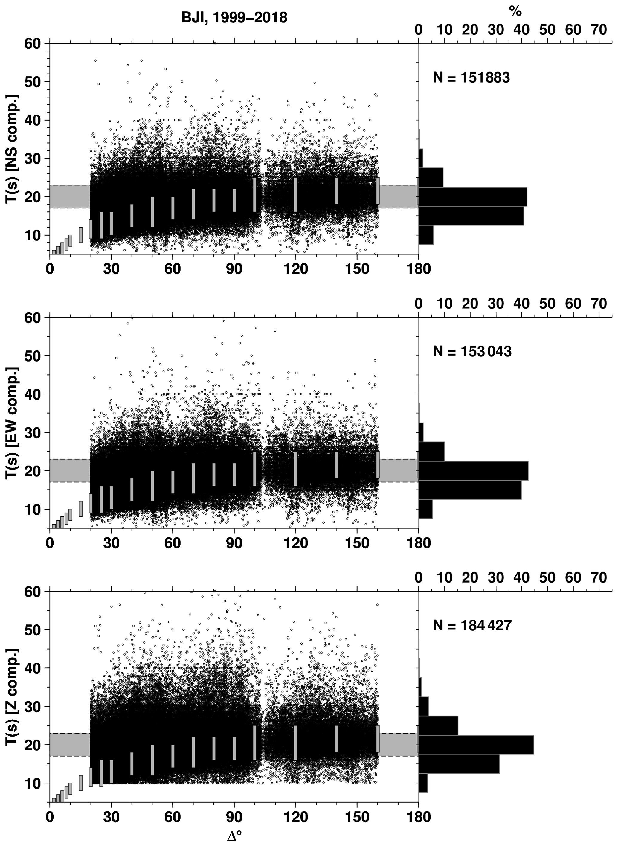
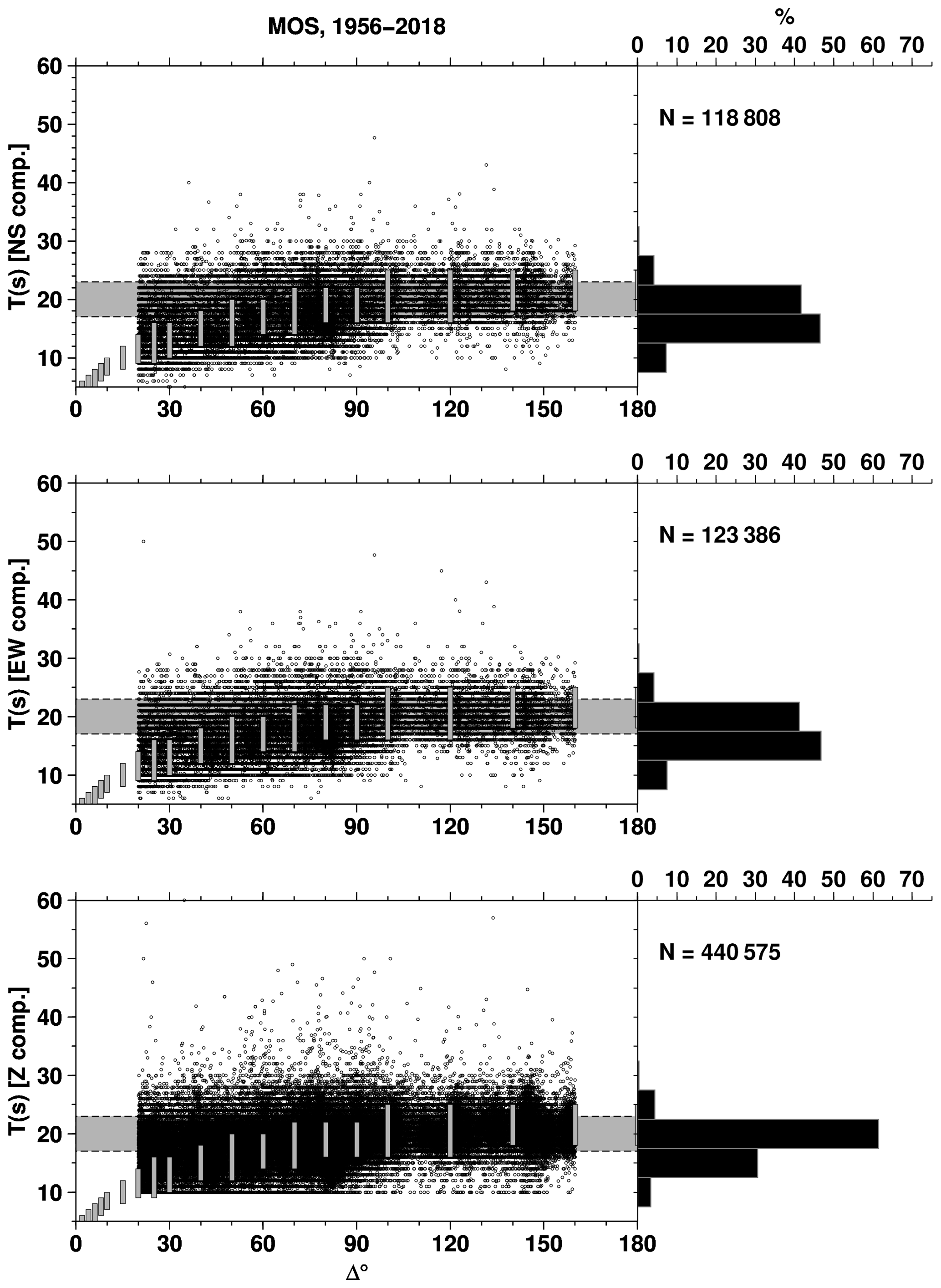
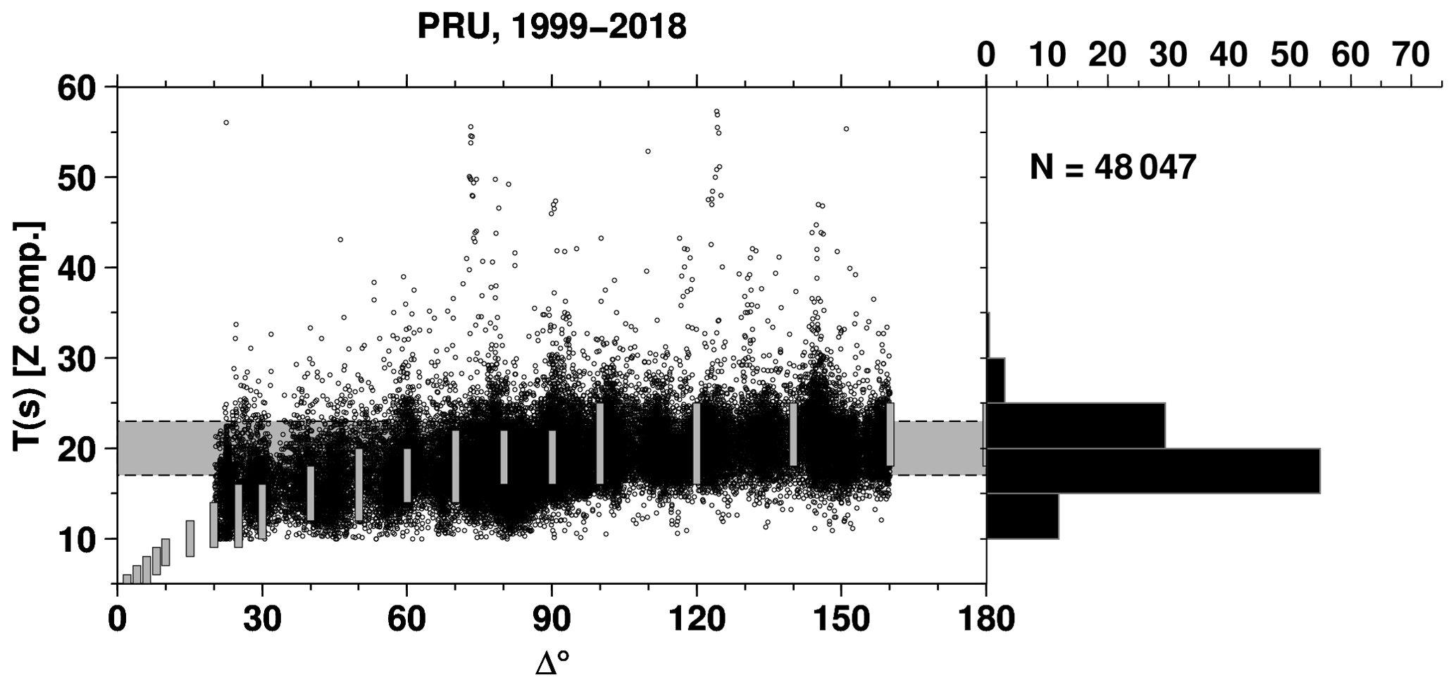
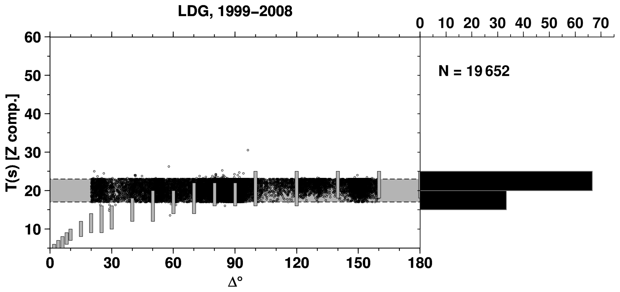
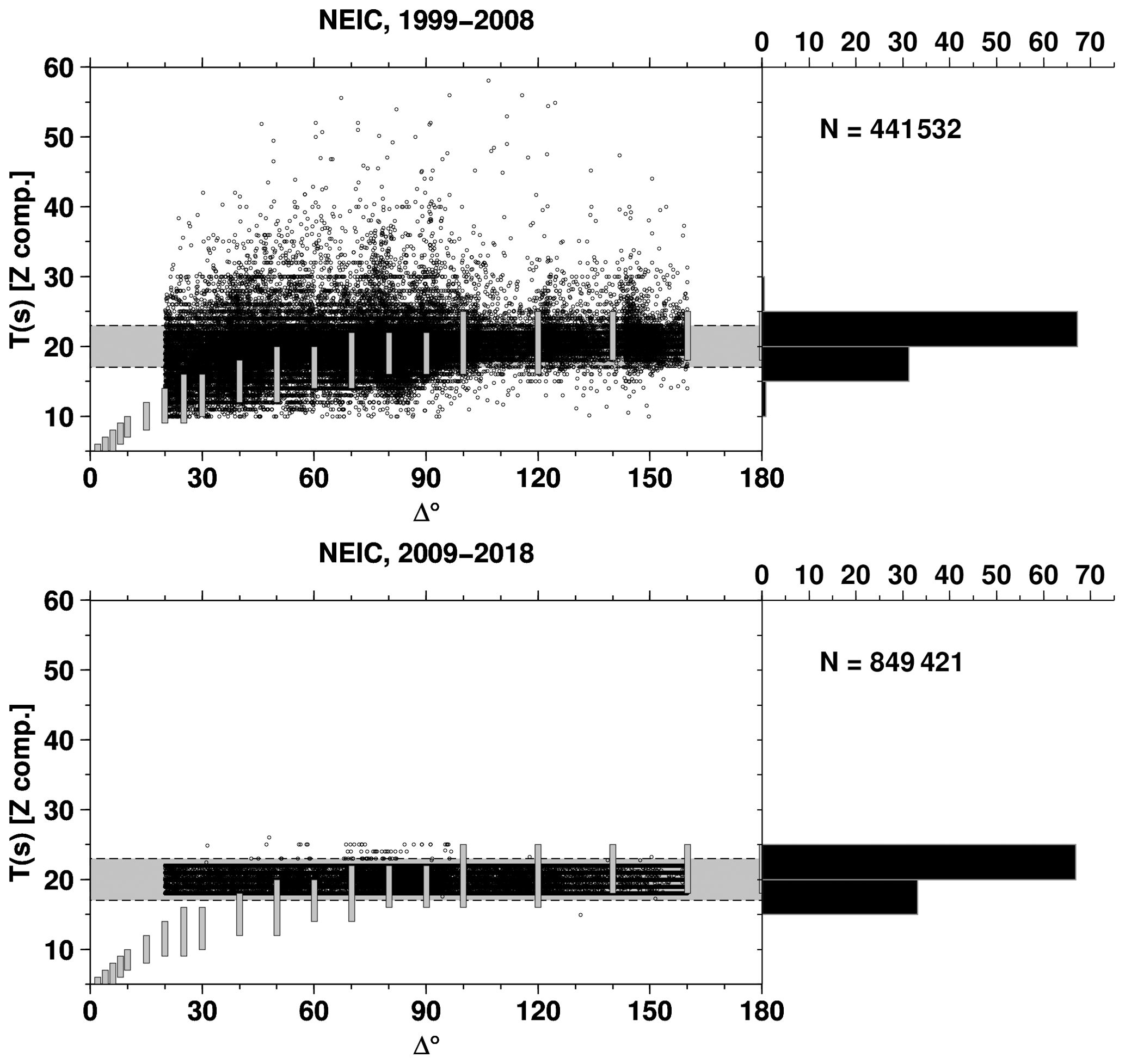
Figure A7 As for Fig. 7 but for reporter NEIC (vertical component only). Here we split the plot in two time periods to emphasize the change in 2009 by NEIC in reporting surface wave amplitudes strictly around 20 s.

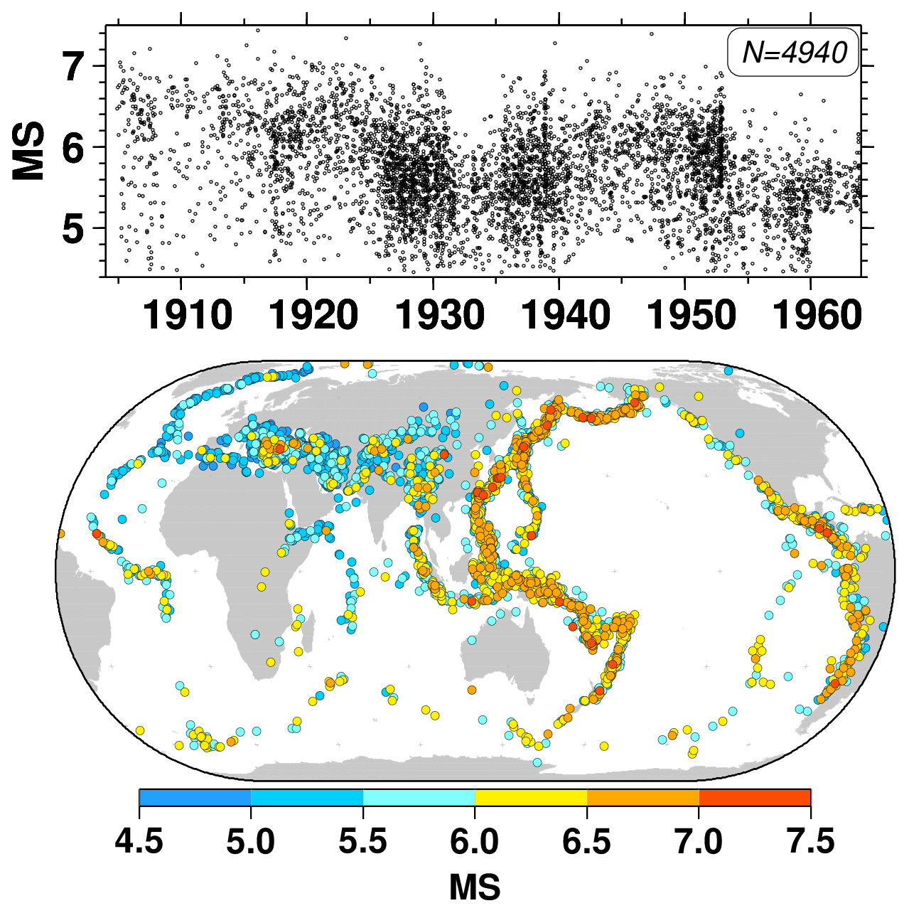
Figure A8 Map colour-coded by M_s and timeline of the pre-1964 earthquakes where, according to our records, M_s has been computed for the first time. Map drawn using the Generic Mapping Tools (GMT) (Wessel et al., 2013) software.