An 11-year record of XCO₂ estimates derived from GOSAT measurements using the NASA ACOS version 9 retrieval algorithm

The Thermal And Near infrared Sensor for carbon Observation – Fourier Transform Spectrometer (TANSO-FTS) on the Japanese Greenhouse gases Observing SATellite (GOSAT) has been returning data since April 2009. The version 9 (v9) Atmospheric Carbon Observations from Space (ACOS) Level 2 Full Physics (L2FP) retrieval algorithm (Kiel et al., 2019) was used to derive estimates of carbon dioxide (CO₂) dry air mole fraction (XCO₂) from the TANSO-FTS measurements collected over its first 11 years of operation. The bias correction and quality filtering of the L2FP XCO₂ product were evaluated using estimates derived from the Total Carbon Column Observing Network (TCCON) as well as values simulated from a suite of global atmospheric inversion systems (models) which do not assimilate satellite-derived CO₂. In addition, the v9 ACOS GOSAT XCO₂ results were compared with collocated XCO₂ estimates derived from NASA's Orbiting Carbon Observatory-2 (OCO-2), using the version 10 (v10) ACOS L2FP algorithm.

These tests indicate that the v9 ACOS GOSAT XCO₂ product has improved throughput, scatter, and bias, when compared to the earlier v7.3 ACOS GOSAT product, which extended through mid 2016. Of the 37 million soundings collected by GOSAT through June 2020, approximately 20 % were selected for processing by the v9 L2FP algorithm after screening for clouds and other artifacts. After post-processing, 5.4 % of the soundings (2×10⁶ out of 37×10⁶) were assigned a “good” XCO₂ quality flag, as compared to 3.9 % in v7.3 (<1 ×10⁶ out of 24×10⁶). After quality filtering and bias correction, the differences in XCO₂ between ACOS GOSAT v9 and both TCCON and models have a scatter (1σ) of approximately 1 ppm for ocean-glint observations and 1 to 1.5 ppm for land observations. Global mean biases against TCCON and models are less than approximately 0.2 ppm. Seasonal mean biases relative to the v10 OCO-2 XCO₂ product are of the order of 0.1 ppm for observations over land. However, for ocean-glint observations, seasonal mean biases relative to OCO-2 range from 0.2 to 0.6 ppm, with substantial variation in time and latitude.

The ACOS GOSAT v9 XCO₂ data are available on the NASA Goddard Earth Science Data and Information Services Center (GES-DISC) in both the per-orbit full format (https://doi.org/10.5067/OSGTIL9OV0PN, OCO-2 Science Team et al., 2019b) and in the per-day lite format (https://doi.org/10.5067/VWSABTO7ZII4, OCO-2 Science Team et al., 2019a). In addition, a new set of monthly super-lite files, containing only the most essential variables for each satellite observation, has been generated to provide entry level users with a light-weight satellite product for initial exploration (CaltechDATA, https://doi.org/10.22002/D1.2178, Eldering, 2021). The v9 ACOS Data User's Guide (DUG) describes best-use practices for the GOSAT data (O'Dell et al., 2020). The GOSAT v9 data set should be especially useful for studies of carbon cycle phenomena that span a full decade or more and may serve as a useful complement to the shorter OCO-2 v10 data set, which begins in September 2014.

1 Introduction

A new era of dedicated satellite observations of greenhouse gases began in 2009, with the successful launch of GOSAT (Kuze et al., 2009). Each day, GOSAT's Thermal And Near infrared Sensor for carbon Observation – Fourier Transform Spectrometer (TANSO-FTS) acquires approximately 10 thousand high-spectral-resolution measurements of reflected sunlight (≃ 36.5×10⁶ in 10 years). Soundings that are determined to be sufficiently clear of clouds and aerosols are processed by retrieval algorithms to produce estimates of XCO₂. Both the quality of the GOSAT TANSO-FTS spectra and the derived XCO₂ estimates have been continually refined over the past 12 years. While the official GOSAT L2 products are available from the National Institute for Environmental Studies (NIES; http://www.gosat.nies.go.jp/en/about_5_products.html, last access: 10 January 2022; Yoshida et al., 2013) a number of independent research institutes have developed their own products (e.g., Butz et al., 2011; Crisp et al., 2012; Cogan et al., 2012; Heymann et al., 2015).

One of these groups, the Atmospheric CO₂ Observations from Space (ACOS) team, used a Level 2 Full Physics (L2FP) retrieval algorithm developed for the NASA Orbiting Carbon Observatory (OCO) to derive estimates of XCO₂ from the GOSAT data (O'Dell et al., 2012; Crisp et al., 2012). Early XCO₂ estimates from these efforts had large biases and random errors when compared to XCO₂ estimates from the Total Carbon Column Observing Network (TCCON) and other standards. For example, the v2.8 ACOS GOSAT L2FP product had biases of 7 to 8 ppm relative to TCCON (Crisp et al., 2012). These biases were reduced to 1–2 ppm in the v2.9 product. The next major release was v3.5 in 2014, which spanned approximately 4 years. This data product showed additional reductions in bias and scatter against TCCON, as well as reasonable agreement in seasonal cycle phase and amplitude (Lindqvist et al., 2015; Kulawik et al., 2016).

These early space-based XCO₂ products were rapidly adopted by the carbon cycle science community. Early studies based on GOSAT ACOS retrievals included Basu et al. (2013), Deng et al. (2014), Chevallier et al. (2014), and Feng et al. (2016). These studies provided the first comprehensive insights into regional flux estimates from space-based observations of carbon dioxide. Houweling et al. (2015) conducted an extensive inter-comparison of the early GOSAT-based atmospheric inversion system studies and reported a reduction in the global land sink for CO₂ and a shift in the terrestrial net uptake of carbon from the tropics to the extratropics. However, these studies also highlighted the role of spatiotemporal systematic errors in the satellite retrievals and the negative impact they can have on estimation of CO₂ sources and sinks using atmospheric inversion systems.

Motivated by these early studies, as well as the launch of the OCO-2 sensor in July 2014, the ACOS team continued to refine the L2FP retrieval algorithm. In 2016, the ACOS GOSAT v7.3 product was distributed. No formal results of the XCO₂ estimates were published by the algorithm team, although internal analysis showed small improvement over v3.5, as well as an extension of the record to 7 years. A number of atmospheric inversion studies were published using the v7.3 product. For example, Chatterjee et al. (2017) and Liu et al. (2017) used v7.3 to define the climatological background in their studies of the impact of the 2015–2016 El Niño on the tropical carbon cycle. Palmer et al. (2019) used this data product in a global study, concluding that the tropical land regions were a net annual source of CO₂ emissions, including unexpectedly large net emissions from northern tropical Africa. Wang et al. (2019) found that the ACOS GOSAT v7.3 XCO₂ yielded a stronger carbon land sink than the v7 OCO-2 product. Byrne et al. (2020) used the ACOS GOSAT 7.3 product to study interannual variability in the carbon cycle across North America, and Jiang et al. (2021) investigated interannual variability of the carbon cycle across the globe with v7.3.

Most recently, the v9 ACOS L2FP retrieval algorithm, first applied to OCO-2 (Kiel et al., 2019), was used to generate estimates of XCO₂ from an 11-year record of GOSAT measurements, spanning April 2009 through June 2020. This both extends the time record over v7.3 and produces an ACOS GOSAT product that is more directly comparable to the newest OCO-2 product, which is now using version 10.

The paper is organized as follows: Sect. 2 discusses the GOSAT TANSO-FTS instrument and measurements as related to the ACOS XCO₂ estimates. In Sect. 3, updates to the ACOS v9 L2FP algorithm are detailed, and an assessment is given of the v9 XCO₂ data product volume. The XCO₂ quality filtering and bias correction procedures, specific to ACOS GOSAT v9, are also discussed. Section 4 provides an evaluation of the v9 XCO₂ product using estimates of XCO₂ from TCCON and from a suite of four atmospheric inversion systems (models). In addition, a comparison to collocated XCO₂ estimates derived from NASA's OCO-2 sensor is presented. A summary of the results is provided in Sect. 6.

2 The GOSAT instrument and measurements

The GOSAT mission is a joint project between the Japan Aerospace Exploration Agency (JAXA), the National Institute for Environmental Studies (NIES), and the Ministry of the Environment (MOE) (Kuze et al., 2009). GOSAT was launched on 23 January 2009 into a sun-synchronous orbit with a local overpass time of approximately 12:49 and a 3 d ground repeat cycle. Its TANSO-FTS collects high-resolution spectra of reflected sunlight that can be analyzed to yield estimates of carbon dioxide (CO₂) (Yoshida et al., 2011, 2013).

2.1 GOSAT TANSO-FTS instrument

TANSO-FTS collects high-resolution spectra of reflected sunlight in the near-infrared (NIR) and shortwave-infrared (SWIR) spectral ranges that include the oxygen A-band near 0.76 µm (ABO2 band) at approximately 0.36 cm⁻¹ spectral resolution, and weak and strong CO₂ absorption features near 1.6 µm (WCO2 band) and 2.0 µm (SCO2 band), respectively, at 0.27 cm⁻¹ spectral resolution. All three channels simultaneously measure two orthogonal components of polarization approximately every 4.6 s.

Each GOSAT sounding has a circular ground footprint with a diameter of approximately 10.5 km when viewing the local nadir. An agile, two-axis pointing system allows cross-track and along-track motions of ± 35^∘ and ± 20^∘, respectively. Before August 2010, a five-point cross-track scan was used, yielding footprints that were separated by approximately 150 km in both the down-track and along-track dimensions. Since that time, a three-point cross-track scan has been used, yielding footprint separation of approximately 260 km (Kuze et al., 2016).

Over water, the TANSO-FTS scan mechanism targets the field of view to collect observations in the direction of the local glint spot, where sunlight is specularly reflected from the surface. Early in the mission, glint observations were collected only within ± 20^∘ of the sub-solar latitude. In May 2013, to increase the latitudinal extent of the GOSAT ocean measurements, the scanning strategy was improved to better track the actual specular glint spot, which varies by latitude and season. The latitude range for glint observation was further extended three times in increments of 3^∘ in September 2014, June 2015, and January 2016, by not only tracking the exact specular point but also tracking along the principal plane of the specular reflection when the glint spot was out of range of the scan mechanism. In addition, more observations over fossil fuel emission target sites such as mega-cities and power plants have been made in recent years, allowing for detailed emission source studies (e.g., Kuze et al., 2020). Daily observation patterns can be found at https://www.eorc.jaxa.jp/GOSAT/currentStatus_10.html (last access: 10 January 2022).

The TANSO-FTS detectors can be read out using independent medium-gain and high-gain signal chains. Most measurements over land use the instrument's high-gain signal chain (H-gain), while brighter land surfaces are measured using the medium-gain signal chain (M-gain) to avoid saturating the detectors. Over oceans, which appear dark in the SWIR spectral bands, measurements are collected using the high-gain signal chain to maximize the signal.

During the first 7 years of GOSAT operations (2009–2015), data acquisition was temporarily suspended due to one spacecraft and two instrument anomalies, as highlighted in Kuze et al. (2016). A rotation failure of a solar paddle in 2014 resulted in a data loss of 6 d. A switch from the primary to secondary pointing mirror in January 2015 resulted in a data loss of approximately 6 weeks, while a temporary shutdown of the cryocooler in August 2015 resulted in a data loss of 13 d.

Since 2015, three additional anomalies interrupted data acquisition. An unexpected shutdown of the instrument occurred in May 2018, resulting in the loss of a week of data. A failure of the second solar panel caused a significant loss of data spanning more than a month in November and December of 2018, and an anomaly of the FTS alignment laser caused a loss of a week of data in June of 2020. In all these cases, the system was able to recover full functionality either through utilization of on-board back-up systems, or through mitigation strategies, and as of the summer of 2021, TANSO-FTS continues to collect science data.

2.2 ACOS GOSAT v9 L1b measurements

The JAXA L1b algorithm, which has been updated more than 10 times over the 11-year data record, produces an internally consistent set of geometrically, radiometrically, and spectrally calibrated TANSO-FTS radiances. The raw spectral measurements are interferograms, which are calibrated and Fourier transformed to yield spectra. The version 205/210 Level 1b (L1b) geolocated and calibrated radiances provided by JAXA have been used for the ACOS v9 reprocessing. A list of L1b updates for v205/210 can be found in Table 3 of the ACOS v9 Data Users Guide (DUG) (O'Dell et al., 2020). Note that while the current L1b version is now 230, the only differences between this version and 205/210 are in the thermal infrared band (5.6–14.3 µm), which is not used in the ACOS XCO₂ retrieval.

After obtaining the calibrated L1b product from JAXA, the ACOS team converts the files to the format needed as input to the ACOS L2 algorithms. The L2FP algorithm uses a simple average of the S and P linear polarizations to produce an approximation of the total measured intensity. Due to cooperation agreements between JAXA and the California Institute of Technology, the distribution of the ACOS GOSAT L1b product is restricted and therefore not publicly available on the NASA DISC. However, the data may be procured by submitting a request to the GOSAT project.

3 The ACOS v9 L2FP XCO₂ retrieval algorithm

The ACOS Level 2 full physics (L2FP) retrieval algorithm is well documented, most recently in O'Dell et al. (2018) for v8 and in Kiel et al. (2019) for v9. A Bayesian optimal estimation framework is used to derive estimates of XCO₂ from spectral measurements of reflected solar radiation. A post-processing step assigns a simple good/bad quality flag (QF) to each XCO₂ value based on successful L2FP algorithm convergence and a series of empirically derived filters. An empirical bias correction (BC) to the estimated XCO₂ values, derived from comparisons with TCCON-derived XCO₂ and CO₂ fields from a suite of atmospheric inversion systems, is included in the Lite File product. Here we provide a summary of the recent evolution of the ACOS algorithm and discuss retrieval parameters and setup specific to GOSAT.

3.1 ACOS L2FP algorithm updates

Table 1 summarizes the evolution of the ACOS L2FP retrieval algorithm from v7 to v10. A similar table, complete through v8, can be found in O'Dell et al. (2018). The trace gas absorption coefficient tables (ABSCO) were updated from v4.2 (Thompson et al., 2012) in ACOS v7 to ABSCO v5.0 (Oyafuso et al., 2017) in ACOS v8/9. The ACOS v9 L2FP algorithm is unmodified relative to v8 (Kiel et al., 2019). However, changes were made in v9 regarding the sampling of the meteorological prior, which does affect ACOS GOSAT estimates of XCO₂. The source of the prior meteorology was switched from the European Center for Medium-range Weather Forecast (ECMWF) in ACOS v7, to the NASA Goddard Modeling and Assimilation Office (GMAO) Goddard Earth Observing System (GEOS) Forward Processing – Instrument Team (FP-IT) product for ACOS v8/9. Both v7 and v8/9 used aerosol priors based on a simple monthly 1^∘ latitude by 1^∘ longitude climatology constructed from the output aerosol fields of the GMAO Modern-Era Retrospective analysis for Research and Applications (MERRA) product (Rienecker et al., 2011). However, between v7 and v8/9, an additional stratospheric aerosol layer was introduced, as described in Sect. 3.1.1 of O'Dell et al. (2018). In addition, the prior value of the aerosol optical depth (AOD) for each retrieved aerosol type was lowered from 0.0375 in ACOS v7 to 0.0125 in ACOS v8/9 based on extensive testing. There was no change in the source of the CO₂ prior from ACOS v7 to v8/9; both versions adopted the prior developed by the TCCON team for use in the ggg2014 algorithm (Wunch et al., 2015). An additional change from ACOS v7 to v8/9 was a switch from a purely Lambertian land surface model to a more sophisticated bi-directional reflectance distribution function (BRDF) model.

Table 1 Updates to recent versions of the ACOS L2FP retrieval algorithm. N/C stands for no change.

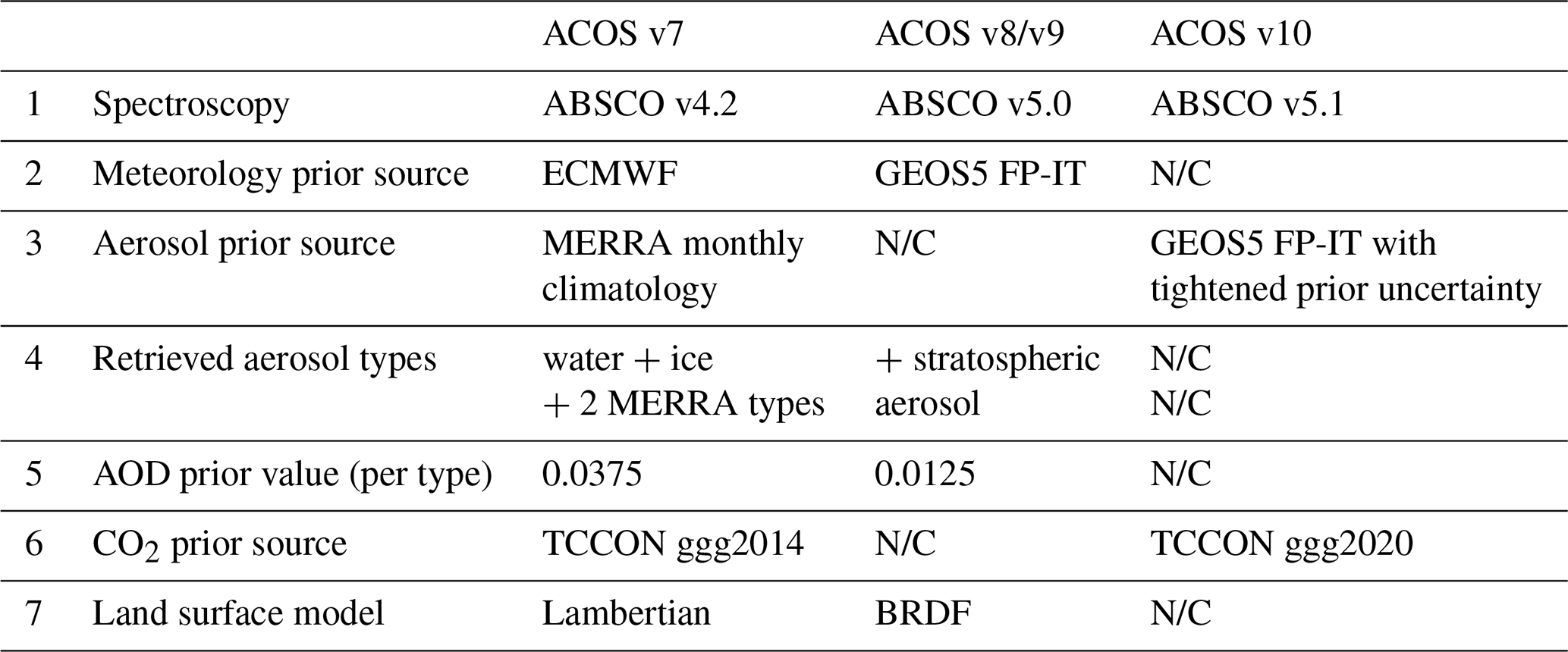
Several important components of the v9 ACOS L2FP retrieval configured for GOSAT have not changed from v7.3: (i) the surface pressure prior constraint remains set at ±2 hPa, (ii) three empirical orthogonal functions (EOFs) are fit in each spectral band (see Sect. 3.3 in O'Dell et al., 2018 for a full discussion of ACOS EOFs), and (iii) a zero level offset (ZLO) is fit in the state vector to account for non-linearity in the ABO2 signal chain on GOSAT TANSO-FTS (Crisp et al., 2012).

To support comparisons of the ACOS GOSAT v9 XCO₂ product with the OCO-2 v10 product, Table 1 includes the most recent updates to the ACOS v10 L2FP algorithm. For v10, the ABSCO tables were again updated from v5.0 to v5.1 (Payne et al., 2020). The aerosol prior was updated from the MERRA monthly climatology to daily GEOS-FT-IT values, with a tightened prior uncertainty (Nelson and O'Dell, 2019). Finally, the CO₂ priors developed by the TCCON team for use in ggg2014 were updated to a revised set of priors developed for use in ggg2020.

3.2 ACOS GOSAT v9 L2FP sounding selection and convergence

GOSAT data from 20 April 2009 through 30 June 2020 were passed through the ACOS L2FP algorithm pipeline, which includes a series of stages where soundings can be rejected or selected for further processing. The throughput of each of these stages for ACOS GOSAT v9 is summarized in Table 2 and Fig. 1. The pipeline begins with a series of preprocessing steps, which reject corrupted spectra and screen the remainder to eliminate those with optically thick clouds and/or aerosols (Taylor et al., 2016). From the full set of measurements (panel a of Fig. 1), the remaining soundings are accepted by the L2FP algorithm (18.8 % of the 37.4×10⁶ measured soundings contained in the ACOS GOSAT v9 record) (panel b of Fig. 1) and a retrieval of XCO₂ is attempted. The majority of the selected soundings successfully converge to a valid solution: 87 % for ACOS GOSAT v9 (16.4 % of the total measured soundings). Soundings can fail to converge for a variety of reasons, including (i) producing non-physical values, such as negative gas mixing ratios or surface pressures (3.9 % of the selected), (ii) converging too slowly and exceeding a predefined number of iterations (3.2 % of the selected), or (iii) having more diverging steps than the predefined maximum (5.9 % of the selected). The 6.1×10⁶ valid soundings were then run through the quality filtering and bias correction procedure discussed in the next section.

Table 2 Accounting of the soundings in the 11-year-long GOSAT ACOS v9 data set at each stage of the data processing chain. The final line summarizes the number of good-quality XCO₂ soundings used in the evaluation section of this work.

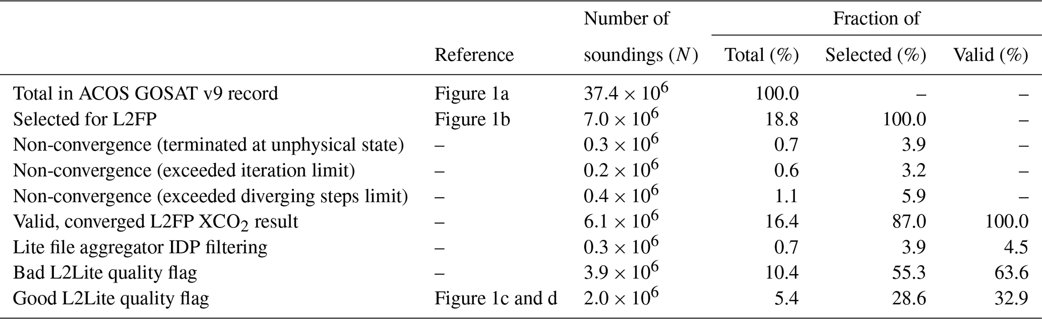
Figure 1 The total measured sounding density per 2.5^∘ by 5^∘ latitude–longitude grid cell in the 11-year (April 2009–June 2020) ACOS GOSAT v9 data record (a). The fraction of the total soundings selected to run through the L2FP algorithm (b). The fraction of the total soundings that converged in the L2FP and were assigned a good L2FP QF (c). The sounding density of the good QF data per 2.5^∘ by 5^∘ latitude–longitude grid cell (d).

3.3 ACOS GOSAT v9 XCO₂ quality filtering and bias correction

All GOSAT soundings that converged to a valid XCO₂ value within the L2FP retrieval were input to the quality filtering and bias correction procedure. A modest fraction (4.5 % of the valid soundings) were removed from the final L2Lite product based on screening via the IMAP-DOAS Preprocessor (IDP) CO₂ ratio, which indicated the presence of clouds or aerosols. Based on a series of screening criteria derived from comparisons with TCCON and modeled CO₂ fields, each sounding that converged within the L2FP is assigned either a “good” (=0) or “bad” (=1) XCO₂ quality flag. Generally, for global or regional studies, it is recommended that users retain only the “good” quality soundings, as the soundings flagged as “bad” quality are likely to include biases that compromise their utility for some applications. A global map of the ACOS GOSAT v9 “good” XCO₂ sounding density is provided in panels C and D of Fig. 1. A subset of data variables from the per-orbit L2Std files (OCO-2 Science Team et al., 2019b), along with the quality filter flag and bias-corrected XCO₂, are repackaged into the daily aggregated L2Lite NetCDF files (OCO-2 Science Team et al., 2019a).

A fundamental aspect of the quality filtering and bias correction procedures (QF/BC) is the need for XCO₂ truth metrics with which to compare the satellite-derived estimates (O'Dell et al., 2018). The development of ACOS GOSAT v9 used XCO₂ truth metrics derived from both TCCON measurements and the median CO₂ distributions determined from a suite of four atmospheric inversion systems, which do not assimilate satellite CO₂ measurements.

TCCON is a well-established validation transfer standard for space-based estimates of XCO₂ (Wunch et al., 2011a, 2017b). For the ACOS GOSAT v9 QF/BC, estimates of XCO₂ derived from TCCON measurements using the ggg2014 retrieval algorithm were used (Wunch et al., 2015). Individual GOSAT soundings were compared to TCCON daily mean XCO₂ values. TCCON data were included if (i) they were flagged as good (flag = 0), (ii) they fell within 3 standard deviations of a daily quadratic fit against time (to remove outliers, e.g., due to unscreened cloud), (iii) they covered at least 15 min within a given day, (iv) there were at least three good soundings within the day, and (v) the standard deviation of the good soundings for the day was less than 3 ppm. In the GOSAT-TCCON comparisons described here, an averaging kernel correction was applied to each TCCON XCO₂ estimate following Nguyen et al. (2014), prior to calculating the daily mean value.

Following the criteria defined in Wunch et al. (2017b), the spatial collocation criteria for GOSAT soundings were those falling within ±2.5^∘ latitude and ±5^∘ longitude of a TCCON station for most sites. For the Southern Hemisphere (SH) sites poleward of 25^∘ S latitude, where the variation of CO₂ is low, the spatial box was increased to ±10^∘ latitude by 20^∘ longitude to increase the number of collocations. For the Edwards TCCON station, which lies in an arid region just north of the polluted Los Angeles metropolitan area, a very specific collocation box of [34.68, 37.46] latitude and [−127.88, −112.88] longitude was used to avoid contamination from the city. Similarly, for the Caltech site, located in Pasadena, California, a latitude box of [33.38, 34.27] and longitude box of [−118.49, −117.55] were used. This avoids collocating GOSAT soundings measured over ocean, the San Gabriel Mountains, and regions too far outside of the Los Angeles basin with the Caltech TCCON data. Finally, only GOSAT soundings acquired within ±2 h of the mean TCCON measurement time were considered. For the quality filtering and bias correction procedure, single sounding level collocations are used to maximize the number of fit points.

Estimates of CO₂ from atmospheric inversion systems, or models, provide a useful metric for evaluating satellite-based estimates of XCO₂ (O'Dell et al., 2018). In this work, a suite of four models (CarbonTracker, CAMS, CarboScope, and University of Edinburgh) were sampled at the GOSAT sounding times and locations. Brief descriptions of each, along with references, are provided in Table 3. The models use a variety of land biosphere prior fluxes, inverse solvers and transport models, and assimilate CO₂ data only from flasks and continuous analyzers on a wide variety of platforms, e.g., observatories, towers, aircraft, and ships. Specifically, no data from GOSAT, OCO-2, or TCCON are assimilated. The CO₂ concentration fields of the models capture the known features of the global atmospheric CO₂ distribution, including seasonality, time trends, and inter-annual variability (IAV) due to El Niño–Southern Oscillation. For each GOSAT sounding, the vertical profiles of CO₂ from the corresponding grid box of each of the four models are spatiotemporally interpolated (linear in latitude, longitude, and time) to the GOSAT observation point, and the GOSAT averaging kernel is applied to each vertical profile to produce a modeled XCO₂ as if viewed from the satellite.

For each GOSAT sounding, a multi-model median (MMM) XCO₂ was calculated from the models having a valid XCO₂ estimate for that location and time. Unless otherwise noted, the model XCO₂ is taken to be that which a perfect OCO-2 would have observed, XCO_2,ak; that is, an averaging kernel correction is applied to account for differences between the model profile of CO₂ and the ACOS prior in the unmeasured part of the profile:

$$\begin{array}{}\text{(1)}& {\mathrm{XCO}}_{\mathrm{2},\mathrm{ak}}=\sum _{i=\mathrm{1}}^{\mathrm{20}}{h}_i\mathit{\{}{a}_i{u}_{\mathrm{m},i}+(\mathrm{1}-a_i\left)u_{\mathrm{a},i}\mathit{\right\}},\end{array}$$

where h_i is the pressure weighting function on the i=1…20 ACOS model levels, a is the normalized ACOS averaging kernel for CO₂, u_m is the model profile of CO₂, and u_a is the ACOS prior profile of CO₂.

To exclude outliers, models with XCO₂ that deviated more than ±1.5 ppm from the initial MMM for that sounding were not included. The sounding was then rejected if more than one of the four models had been excluded, or if the standard deviation amongst the valid models was > 1 ppm. Approximately 85 % of the GOSAT v9 soundings with a good L2FP quality flag had a valid MMM XCO₂ value for analysis. The regions with the highest fraction of rejections occur along the Southern Ocean (latitude −60^∘), the Amazon and Congo rain forests, and a broad region across northern Asia. Table 4 lists the model version numbers used for the QF/BC procedure, as well as that used in the evaluation of the final good-quality XCO₂ product that will be presented later.

Peters et al. (2007)CarbonTracker (2021)Rödenbeck (2005); Rödenbeck et al. (2018)CarboScope (2021)Chevallier et al. (2010)CAMS (2021)Feng et al. (2009)UoE (2021)

Table 3 Carbon inversion systems used for ACOS GOSAT v9. NOAA – National Oceanic Atmospheric Administration, CASA – Carnegie–Ames–Stanford Approach, TM5 – Transport Model 5, TM3 – Transport Model 3, EnKF – ensemble Kalman filter, 4D-Var – 4-Dimensional Variation, ORCHIDEE – Organising Carbon and Hydrology In Dynamic Ecosystems, LMDZ – Laboratoire de Météorologie Dynamique, UoE – University of Edinburgh, GEOS-Chem – Goddard Earth Observing System Chemistry.

Palmer et al., 2019

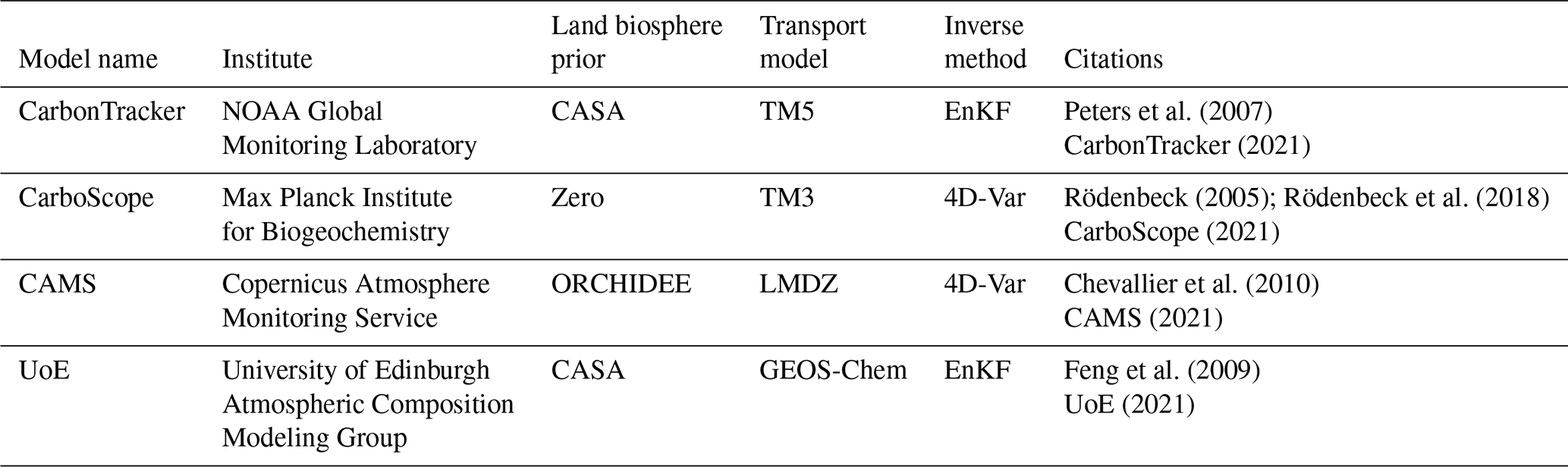
Table 4 Carbon inversion system data sets used for the QF$/$BC and XCO₂ evaluation of ACOS GOSAT v9.

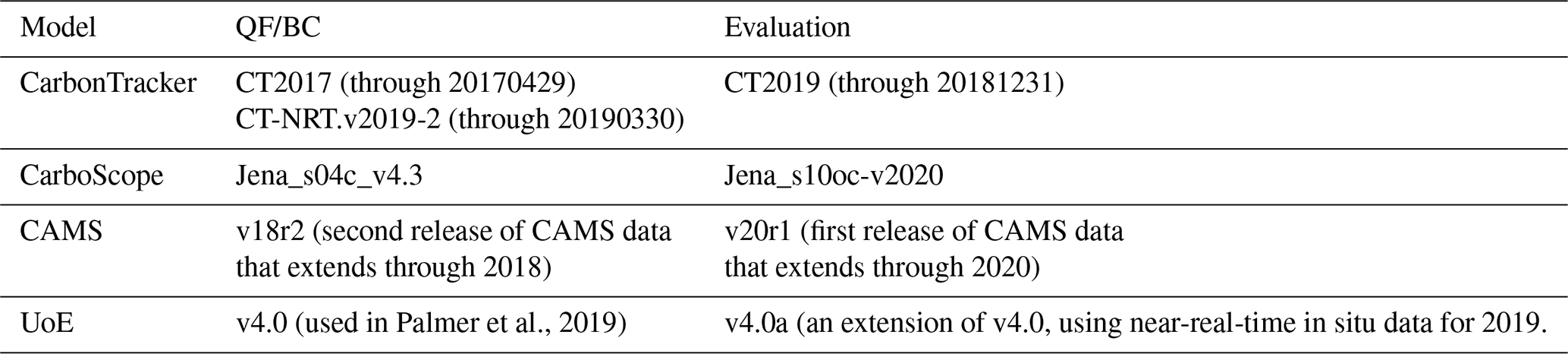
Table 5 lists the quality filtering variables used for ACOS GOSAT v9 and their corresponding thresholds. Many of the same variables (18 out of 31) were also used in the OCO-2 v9 quality filtering, as seen in Table 5 of Kiel et al. (2019). This includes the IDP CO₂ and H₂O ratios (Frankenberg et al., 2005), and the A-band preprocessor dP, i.e., the difference between the retrieved and prior surface pressure from the oxygen A band (Taylor et al., 2016). Another common variable used for quality filtering is the perturbation in the L2FP CO₂ vertical profile relative to the prior, a quantity called “CO₂ grad del” (δ ${\mathrm{\nabla }}_{{\mathrm{CO}}_{\mathrm{2}}}$), as defined in Eq. (5) of O'Dell et al. (2018). A number of aerosol-related retrieval parameters are also used, similar to OCO-2 v9. Section 2.5 of the ACOS GOSAT v9 DUG provides additional details on the quality filtering (O'Dell et al., 2020).

Table 5 ACOS GOSAT v9 L2FP quality filtering variables and thresholds. Descriptions of the variables can be found in the DUG (O'Dell et al., 2020). Soundings falling outside of the data ranges are assigned a bad XCO₂ quality flag. The second column identifies variables that were also used for OCO-2 v9 quality filtering, as taken from Table 5 of Kiel et al. (2019).

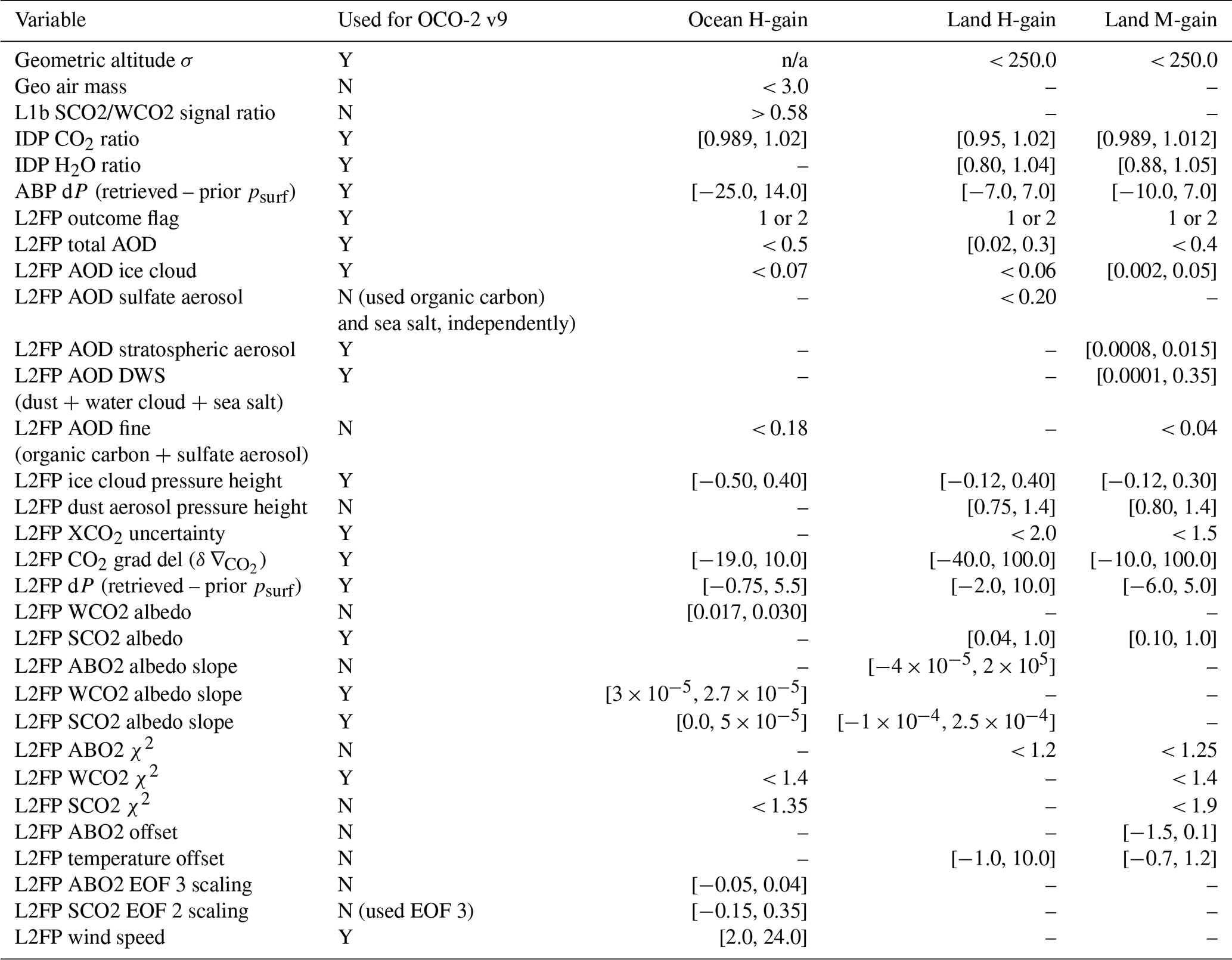
n/a – not applicable

Spurious correlations in the estimates of XCO₂ with other retrieval variables due to inadequacies in the modeled physics motivate the application of a bias correction (Wunch et al., 2011b; O'Dell et al., 2018). Generally such spurious correlations are found with state vector elements such as retrieved surface pressure, various aerosol parameters, and δ ${\mathrm{\nabla }}_{{\mathrm{CO}}_{\mathrm{2}}}$. For each sensor there are also typically offsets by viewing mode, e.g., land glint versus ocean glint, which are accounted for via the bias correction. A general discussion of the ACOS XCO₂ bias correction methodology is provided in Sect. 4 of O'Dell et al. (2018), where the fundamental equation is defined as

$$\begin{array}{}\text{(2)}& {\mathrm{XCO}}_{\mathrm{2},\mathrm{bc}}={\displaystyle \frac{{\mathrm{XCO}}_{\mathrm{2},\mathrm{raw}}-{\mathrm{C}}_{\mathrm{P}}\left(\mathrm{mode}\right)-{\mathrm{C}}_{\mathrm{F}}\left(j\right)}{{\mathrm{C}}_{\mathrm{0}}\left(\mathrm{mode}\right)}},\end{array}$$

where C_P is the mode-dependent parametric bias, C_F is a footprint-dependent bias for footprints 1…8, and C₀ represents a mode-dependent global scaling factor. Note that for GOSAT there is no footprint-dependent bias correction term, as is necessary for OCO due to low-level calibration errors across the detector frame. Further, to be consistent with previous ACOS GOSAT data versions, the global divisor is replaced by an additive offset, which is effectively the same because the range of XCO₂ variability (∼ 20 ppm) is small relative to the mean XCO₂ (∼ 400 ppm).

The explicit formula for application of the ACOS GOSAT v9 correction is provided in Sect. 2.5.6 of the DUG (O'Dell et al., 2020). For both land H-gain and M-gain, a set of five BC variables are used, while ocean H-gain uses only three variables. The difference between the H-gain and M-gain bias correction over land is minor. New for ACOS GOSAT v9 is the use of a correction against time, which is made possible with an 11-year data record; the corrections are 0.05 ppm/yr over land and 0.10 ppm/yr over water. The source of this spurious drift in the bias-corrected XCO₂ is currently unclear and is the subject of ongoing study. Although there is some commonality in the quality filtering and bias correction variables used for ACOS GOSAT v9 (compare Tables 5 and 6), they do differ somewhat, as is typically the case with each sensor and data version.

Table 6 compares the bias correction variables used for ACOS GOSAT v9 with the variables used in the previous ACOS GOSAT v7.3, as well as with OCO-2 v9 and v10. The same few variables have appeared in all recent versions, including L2FP δ ${\mathrm{\nabla }}_{{\mathrm{CO}}_{\mathrm{2}}}$, L2FP dP, and L2FP DWS for land soundings. For ocean soundings the bias correction variables have evolved, with the only common one being δ ${\mathrm{\nabla }}_{{\mathrm{CO}}_{\mathrm{2}}}$.

Kiel et al. (2019)

Table 6 ACOS L2FP bias correction variables by sensor and product version.

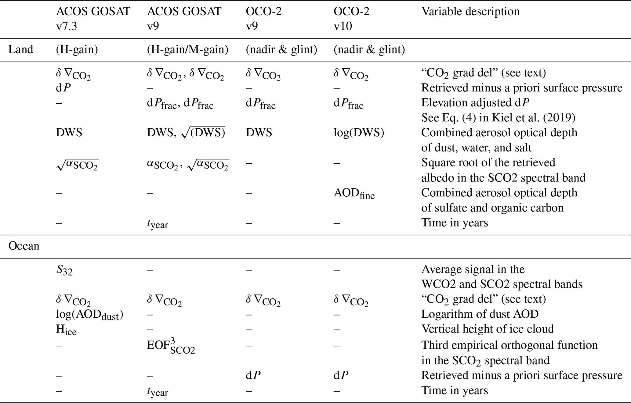
Table 7 summarizes the effect of the quality filtering and bias correction on the ACOS GOSAT XCO₂ for v7.3 and v9. For ocean H-gain soundings, the v9 quality flag is substantially more restrictive compared to v7.3, i.e., ≃ 57 % pass rate compared to ≃ 78 %. This is mostly driven by the more extensive latitudinal coverage in the v9 record, which tends to include more soundings with high solar zenith angles (SZA) and low signal-to-noise ratio (SNR), which are more challenging for the L2FP. For H-gain land observations, the two versions have quite similar QF pass rates (≃ 35 %–45 %). The QF pass rate for v9 M-gain land data is ≃ 39 % when compared against models but ≃ 56 % against TCCON. In all cases there is a significant reduction in the scatter of the XCO₂ after application of the QF/BC: by a factor of ≃ 2 for ocean H-gain and land M-gain and a factor of 3 for land H-gain. The QF/BC scatter is always slightly lower for v9 compared to v7.3, even though the number of soundings is greater by 1.5 to 10 times for the various scenarios.

Table 7 Comparison of ACOS GOSAT v7.3 versus v9 sounding throughput and XCO₂ scatter against truth metrics before and after filtering and bias correction.

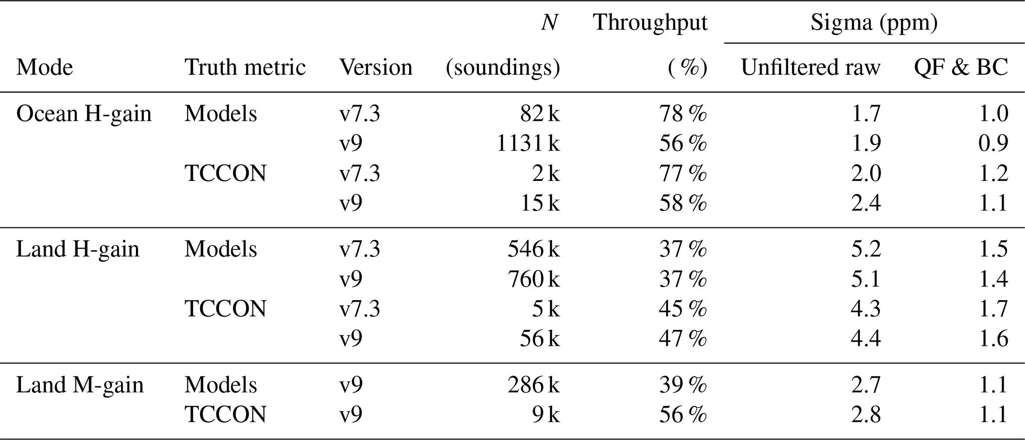
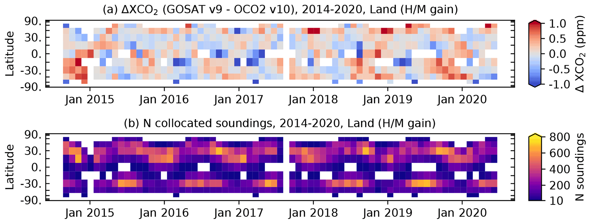
Figure 2 shows the relative magnitudes of the bias correction on the good-quality soundings by season, aggregated to 2.5^∘ latitude by 5^∘ longitude. The global median bias of −1.8 ppm has been removed for clarity. This highlights gradients and contrasts in the bias correction, which are of importance as gradients in CO₂ concentrations are the primary driver of CO₂ fluxes in atmospheric inversion systems. In general, the bias correction is necessary to remove spurious contrasts between land and ocean XCO₂ values. The strongest relative bias corrections are positive adjustments over the bright land surfaces in M-gain viewing mode, specifically the Sahara in DJF and JJA and Australia in DJF. The land H-gain observations have a mix of relative bias correction values, ranging from mildly negative over high northern latitudes in JJA to moderately positive over northern mid-latitudes in JJA in the western United States and the Middle East. Most of the ocean H-gain observations have a mildly negative relative bias correction, with some mild positive values in the southern tropical oceans in DJF.

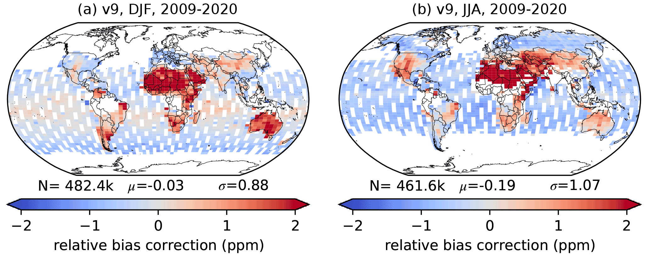
Figure 2 Maps of ACOS GOSAT v9 relative bias correction for DJF (a) and JJA (b) for good QF soundings in the 11-year data record at 2.5^∘ by 5^∘ latitude–longitude, after removal of the global, median bias of −1.8 ppm. Grid cells with fewer than five GOSAT soundings are not colored. The total number of soundings (N), and the mean bias (μ) and standard deviation of the bias (σ) in each grid cell are given.

4 Evaluation of ACOS GOSAT v9 XCO₂

The ACOS GOSAT v9 XCO₂ record was characterized in five ways: (i) an analysis of the XCO₂ “good-quality” data volume, (ii) a spatiotemporal analysis of the XCO₂ estimates, (iii) a validation against XCO₂ estimates from TCCON, (iv) a comparison to XCO₂ derived from models, and (v) a comparison with collocated XCO₂ estimates from the OCO-2 v10 product.

4.1 ACOS GOSAT v9 “good-quality” data volume

It is instructive to compare the ACOS GOSAT v9 product to the earlier v7.3 product to highlight similarities and differences in the quality filter screening. A time series histogram of the monthly throughput of the good-quality-filtered soundings for the v9 product compared to v7.3 is shown in Fig. 3. The soundings have been binned by month, with the three GOSAT observation modes displayed by color. The v7.3 product did not contain any land M-gain data in the L2Lite files (red in the figure) as the quality filtering and bias correction were not developed for that gain mode in v7.3 due to some unreconciled differences. An important feature of the v9 data record is the extension in time, which runs through June 2020, compared to a termination date of June 2016 for v7.3. Even for the overlapping v7.3 and v9 time period (2009 through mid 2016), there are some differences in the data volume for land H-gain and ocean H-gain observations. This is due to changes in both the details of the QF procedure, including changes in the variable thresholds used to assign QF = good/bad, and to some differences in the convergence characteristics of the L2FP retrieval. Generally, v9 is producing up to 60 % more good-quality data than v7.3 near the end of the overlap period in 2016. There was a substantial increase in the number of good QF soundings from 2010 to 2019, due to the increased latitudinal range of the ocean observations as a result of improvements in the GOSAT pointing strategy, as well as improvements in the sounding selection for ACOS L2FP v9.

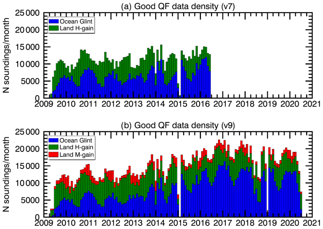
Figure 3 Time series histograms of the monthly number of good QF GOSAT soundings for v7.3 (a) and v9 (b) spanning the 11-year record. The large data gaps in early 2015 and 2019 were caused by a switch from the primary to secondary pointing mirror and a solar panel failure, respectively.

Figure 4 shows sounding density Hovmöller plots comparing ACOS GOSAT v7.3 (a) to v9 (b) with the three GOSAT observation modes combined. Again, the extended time period covered by v9 is evident. The increase in sounding density in the SH beginning in 2016 due to optimization of the GOSAT viewing strategy is prominent in the v9 product. This feature is also seen in the spatial maps showing the fraction of good-quality soundings and the density per grid box, in panels (c) and (d) of Fig. 1, which was introduced in Sect. 3.2. Persistently clear regions, such as the Sahara and the western part of Australia, have as many as 30 % of the observations assigned a good-quality flag. Large regions of the tropical Pacific and Atlantic also contain a relatively high fraction of good-quality soundings. On the other hand, tropical forests and high latitudes in general have low yields of good-quality soundings. This is largely a combination of cloud contamination, dark surfaces at shortwave infrared wavelengths, and low solar illumination conditions, all three of which are problematic for retrieving CO₂ from space using reflected sunlight.

Figure 4 Sounding density comparing v7.3 (a) to v9 (b) good QF data as a function of time and latitude at 30 d by 15^∘ latitude resolution for all viewing modes combined.

4.2 ACOS GOSAT v9 XCO₂ spatiotemporal analysis

There has been a steady increase in the atmospheric burden of CO₂ since the onset of the industrial age due mainly to the burning of fossil fuels (e.g., Keeling et al., 1995). In May of 2009, at the beginning of the GOSAT mission, the mean global value of XCO₂ reported by the NOAA Global Monitoring Laboratory was 387.95 ppm, while by May of 2020, the mean global value had risen to 413.81 ppm (Dlugokencky and Tans, 2021). This yields a secular increase of ≃ 2.35 ppm/yr. For comparison, Fig. 5 shows the ACOS GOSAT v9 bias-corrected and quality-filtered XCO₂ as a function of latitude (15^∘ increments) and time (30 d increments) for combined land M and H-gain observations (a) and ocean H-gain observations (b). Using the monthly mean XCO₂ values (combined land and ocean) for May 2009 (386.50 ppm) and May 2020 (411.82 ppm), the ACOS GOSAT v9 record has a secular increase of ≃ 2.30 ppm/yr over the 11-year record. This small disagreement in secular trend of approximately 2 % is understandable, given the significant differences in the spatiotemporal sampling of the two data sets. For the interested reader, a thorough comparison of satellite- and surface-derived growth rates in atmospheric CO₂ is given in Buchwitz et al. (2018).

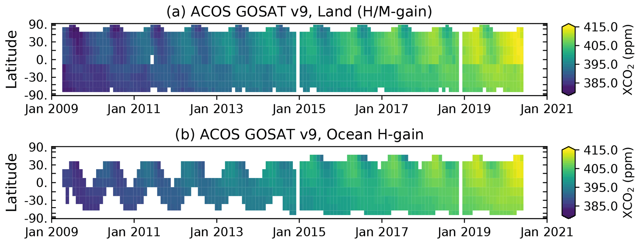
Figure 5 ACOS GOSAT v9 bias-corrected and quality-filtered XCO₂ as a function of latitude (15^∘ increments) and time (30 d increments) for combined land M-gain and H-gain observations (a), and ocean H-gain observations (b). Grid cells with fewer than 10 GOSAT soundings are not colored.

The maps in Fig. 6 show the spatial distribution of XCO₂ at 2.5^∘ latitude by 5^∘ longitude resolution for 2010 (top) and 2019 (bottom), for DJF (left) and JJA (right). The dynamic range of the color scale in each case is 6 ppm. However, due to the secular increase in global CO₂ of ≃ 2.3 ppm per year, the scale is centered ≃ 20 ppm higher in 2019 compared to 2010. The strong latitudinal gradients in XCO₂ are similar in these two seasons, while the zonal gradient tends to be weakest in MAM (not shown), just before the summer drawdown of CO₂ by the land biosphere begins. The increase in the number of ocean H-gain soundings in the later part of the data record is also evident in these maps.

Qualitatively, the patterns in the maps look quite similar from 2010 to 2019, but with increased data coverage. In general, the highest concentrations of XCO₂ for the two selected seasons are observed by GOSAT in the Northern Hemisphere (NH) during DJF, especially over northern tropical Africa (between 0 and 15^∘ N latitude), large portions of China, and the eastern United States. This stands to reason, as the atmospheric burden of CO₂ increases towards a peak during NH winter due to inactivity of the land biosphere, coupled with strong anthropogenic CO₂ emissions. During DJF the ACOS GOSAT v9 XCO₂ exhibits relatively low concentrations across the entire SH, as would be expected if the Southern Ocean were a strong carbon sink (e.g., Gruber et al., 2019). In JJA, the XCO₂ is reduced over the mid-latitude and boreal forests, also expected behavior due to strong photosynthetic uptake of CO₂ during this season (e.g., Ciais et al., 2019).

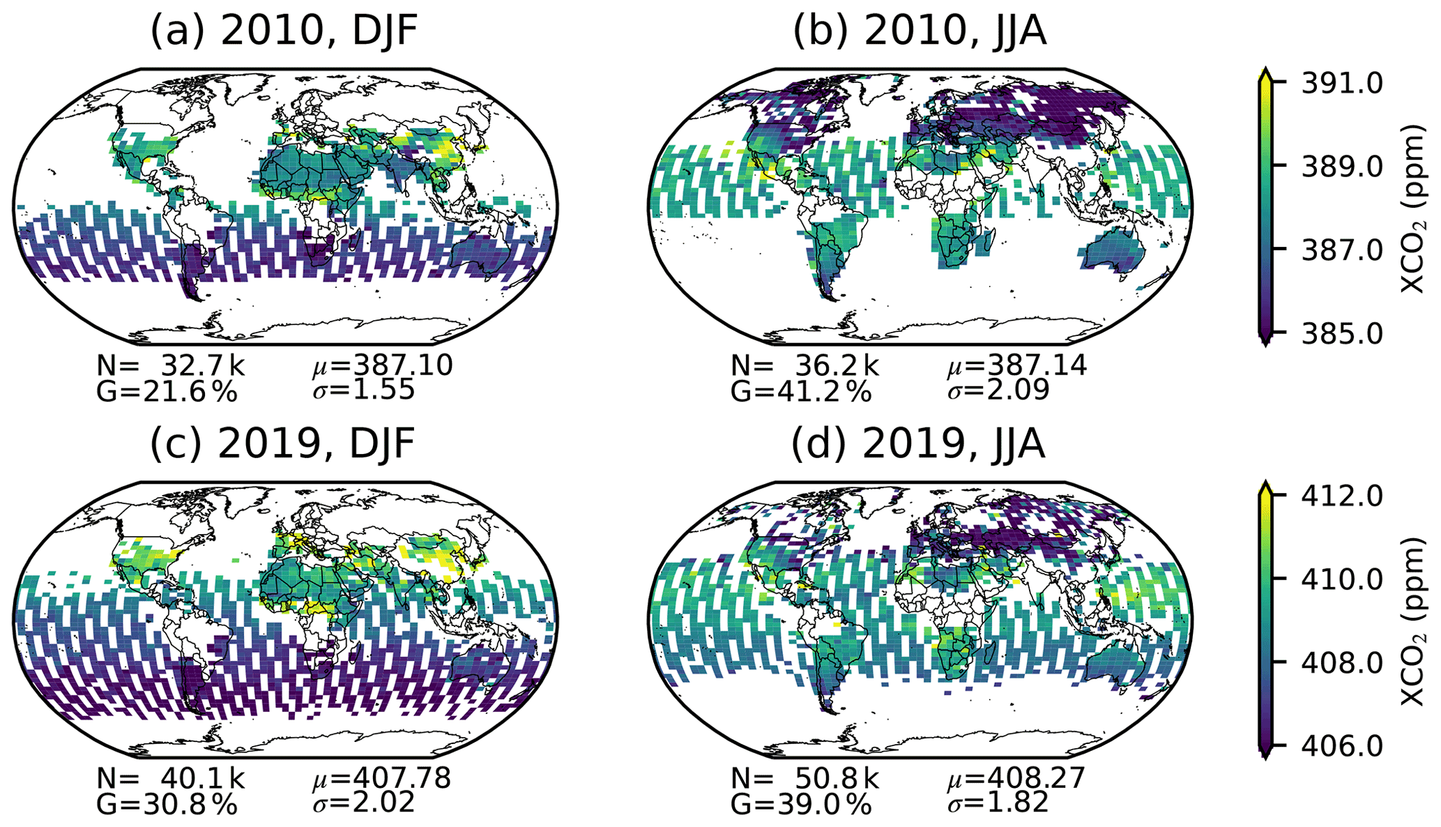
Figure 6 ACOS GOSAT v9 bias-corrected XCO₂ for the good QF soundings at 2.5^∘ latitude by 5^∘ longitude resolution for DJF 2009–2010 (a), JJA 2010 (b), DJF 2018–2019 (c), and JJA 2019 (d). The dynamic range of the color scale in each case is 6 ppm. However, due to the secular increase in global CO₂ of ≃ 2.2 ppm per year, the scale is centered ≃20 ppm higher in 2019 compared to 2010. Grid cells with fewer than five GOSAT soundings are not colored.

A quantification of differences in the bias-corrected ACOS GOSAT v9 XCO₂ data product relative to the v7.3 product is given in Fig. 7 for the overlapping period. The top row (panels a through c) shows results for the land H-gain observations, while the lower row (panels d through f) shows results for the ocean H-gain observations. Only soundings that were present in both data sets and assigned a good-quality L2FP flag were used in this comparison. This restricts the analysis to April 2009 through June 2016 and also eliminates the v9 land M-gain data, as no M-gain data exist in the v7.3 product. The mean and standard deviation of the ΔXCO₂ for the approximately 311 k land soundings at the single sounding level are −0.18 and 0.72 ppm, respectively, as shown in panel (a). When gridded and mapped at 2.5^∘ latitude by 5^∘ longitude resolution, as shown in panel (b), the majority of the negative signal (v9 XCO₂ lower than v7.3) occurs at latitudes greater than approximately 45^∘. Most of the land mass at latitudes less than 45^∘ has ΔXCO₂ values closer to zero, with the largest positive signals appearing over equatorial forests. Furthermore, when the data are gridded and viewed versus time and latitude in 30 d by 15^∘ increments, respectively, as in panel (b), we see that the ΔXCO₂ signal has an increasing tendency in time; i.e., the v9 XCO₂ increases more rapidly in time than v7.3. The cause of this effect is currently unknown, but it is partially due to the implementation in v9 of a time-dependent bias correction term of +0.05 ppm/yr for land observations. This translates into an expected change of about 0.35 ppm in the v9 record over the 2009 to 2016 time span.

For the ocean H-gain observations at the single sounding level (panel d), the mean and standard deviation of the ΔXCO₂ are +0.28 and 0.79 ppm, respectively. When gridded and mapped at 2.5^∘ latitude by 5^∘ longitude resolution (panel e), the spatial distribution is fairly smooth, i.e., low variation in both latitude and longitude. Finally, when the data are gridded versus time and latitude (panel f), the modest variation in latitude is confirmed, but a substantial time dependence is observed, with the ΔXCO₂ signal beginning negative in 2009 (v9 XCO₂ lower than v7.3), and switching to a positive ΔXCO₂ signal by 2016 (v9 XCO₂ higher than v7.3). The time-dependent bias correction term for ocean H-gain observations was +0.1 ppm/yr. This translates into an expected change of about 0.7 ppm over the 2009 to 2016 time span in the v9 record, accounting for some but not all of this time-dependent difference between v9 and v7.3.

This direct comparison between the v9 and v7.3 XCO₂ product only allows for statements as to their differences. It does not allow one to deduce which is closer to truth. Therefore, an analysis of the v9 XCO₂ data product against truth metrics follows. Furthermore, it is difficult to accurately determine the effect that the new v9 XCO₂ product will have on atmospheric inversion system results relative to v7.3 without further detailed study.

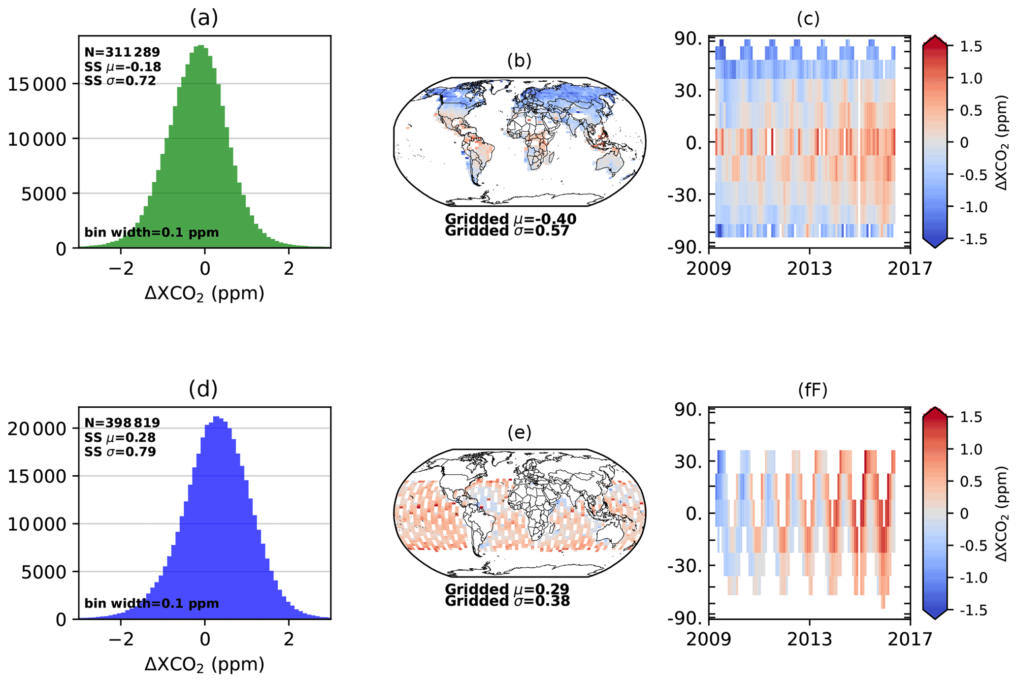
Figure 7 Analysis of the ACOS GOSAT calculated ΔXCO₂ (v9 minus v7.3) for the quality-filtered and bias-corrected soundings for the overlapping period spanning April 2009 through May 2016. Panels (a) through (c) show results for the land H-gain observations, while panels (d) through (f) show results for ocean H-gain observations. Panels (a) and (d) show the single sounding frequency distribution of ΔXCO₂ in 0.1 ppm bins. Panels (b) and (e) show the spatially gridded ΔXCO₂ at 2.5^∘ latitude by 5^∘ longitude resolution. Panels (c) and (f) show the ΔXCO₂ as a function of time and latitude in 30 d by 15^∘ increments, respectively. The statistics in panels (a) and (d) were calculated at the single sounding level, while those reported in panels (b) and (e) were calculated on the grid box means.

4.3 ACOS GOSAT v9 XCO₂ versus TCCON

A list of TCCON stations used in this work, including basic physical information and data citations, is given in Table 8. For the evaluation against the ACOS v9 XCO₂ data, the single sounding collocations described in Sect. 3.3 were aggregated into overpass mean values. Essentially the same TCCON data set was used for both the QF$/$BC procedure as for the evaluation, as no hold-over data were maintained. Also, as described in Sect. 3.3, an averaging kernel correction was applied to the TCCON data in order to fairly compare to the satellite data. A one-to-one linear regression of the XCO₂ provides a simple quantification of the agreement, as shown in Fig. 8.

Strong et al. (2019)Kivi et al. (2014)Wunch et al. (2017a)Deutscher et al. (2019)Notholt et al. (2019)Hase et al. (2015)Te et al. (2014)Warneke et al. (2019)Sussmann and Rettinger (2018a)Sussmann and Rettinger (2018b)Wennberg et al. (2017)Morino et al. (2016)Iraci et al. (2016b)Wennberg et al. (2016b)Dubey et al. (2014); Lindenmaier et al. (2014)Goo et al. (2014)Morino et al. (2018a)Petri et al. (2020)Iraci et al. (2016a)Wennberg et al. (2016a)Wennberg et al. (2016a)Wennberg et al. (2015)Kawakami et al. (2014)Liu et al. (2018)Blumenstock et al. (2017)Morino et al. (2018b)Feist et al. (2014)Griffith et al. (2014a)De Mazière et al. (2017)Griffith et al. (2014b)Pollard et al. (2019)

Table 8 List of TCCON stations used in the BC$/$QF and XCO₂ evaluation of ACOS GOSAT v9, along with the data citations.

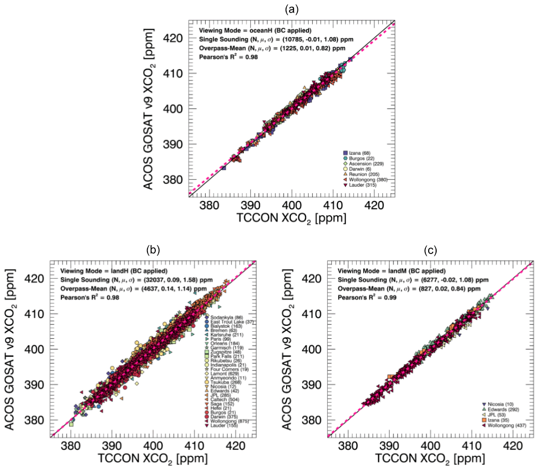
Figure 8 Quality-filtered and bias-corrected ACOS GOSAT v9 vs. collocated TCCON XCO₂ for ocean H-gain (a), land H-gain (b), and land M-gain (c). Each point represents an overpass mean, which typically contain 5–10 GOSAT soundings per overpass. The legend in the lower right indicates the number of collocated overpass means for individual TCCON stations. Summary statistics for all stations combined are reported in the upper left of each panel for both single sounding and overpass means.

For ocean H-gain observations (Fig. 8a), the mean (μ) of the differences in XCO₂ (ΔXCO${}_{\mathrm{2}}^{\mathrm{TCCON}}$ = GOSAT − TCCON) is essentially zero: −0.01 ppm for the single-sounding (SS) results and +0.01 ppm for the overpass mean (OPM) results. The corresponding standard deviations (σ) are 1.08 and 0.82 ppm for the SS and OPM results, respectively. This indicates that roughly half of the SS error variance is a result of instrument noise or other random high-frequency error sources (1.08²=1.2 ppm versus 0.82²=0.7 ppm).

For land H-gain observations (Fig. 8b), $\mathit{\mu }=+\mathrm{0.09}$ ppm and +0.14 ppm for the SS and OPM, respectively. The land H-gain σ values are higher than for ocean H-gain: 1.58 and 1.14 ppm for SS and OPM, respectively. Larger variations in ΔXCO${}_{\mathrm{2}}^{\mathrm{TCCON}}$ are expected for land H-gain due to variability in topography and surface brightness, as well as higher likelihood of contamination by cloud and aerosol, all of which are more challenging for the ACOS retrieval. Further, biology and atmospheric transport cause CO₂ signals to vary more over land regions, and in addition, instrument noise is higher because the SNRs tend to be lower.

Land M-gain observations have near-zero bias ($\mathit{\mu }=-\mathrm{0}$.02 ppm and +0.02 ppm for SS and OPM, respectively) and scatter similar to that for ocean H-gain (σ=1.08 and 0.84 ppm for SS and OPM, respectively), likely driven by lower variability in surface topography and brightness compared to land H-gain observations, as well as higher SNRs over these bright land surfaces.

The correlation in the XCO₂ between the data sets in all observation modes is high, with Pearson R²=0.98, 0.98, and 0.99 for ocean H-gain, land H-gain, and land M-gain, respectively. Overall, these results indicate excellent agreement between the bias-corrected and quality-filtered ACOS GOSAT v9 XCO₂ product and collocated estimates from TCCON.

Figure 9 shows the mean absolute error (MAE) between the overpass mean collocated GOSAT and TCCON XCO₂, organized by latitude bins, season, and observation mode for v7.3 (panels a and b) and v9 (panels c, d, e). The calculation of the MAE and error bars follow the procedure reported in Chatterjee et al. (2013) (Eqs. 3 and 4). The error bars on the MAE represent the scatter around the mean. A smaller error bar, or a lower scatter, implies that the MAE values are more consistent across a group of TCCON stations within a latitude band and season. The MAEs tend to be lower for v9 compared to v7.3, with smaller error bars and increased number of collocations. This is especially true for the SH ocean H-gain data, where the MAE ranges from 0.4 to 0.7 ppm in v9 for all seasons, in contrast to v7.3, which had higher MAE ranging from 0.5 to 0.85 ppm in that region. In the v9 land H-gain data, the MAE is roughly a function of latitude, with the highest values (≃ 1.0 ppm) seen between 60–90^∘ N and the lowest values (≃ 0.7 ppm) seen from 30–60^∘ S. This stands to reason as lower variability of XCO₂ in the SH tends to yield better agreement between satellite- and ground-based observations. The error bars on the v9 land H-gain estimates in the 30–60^∘ N latitude range are very small, due in part to the large number of collocations. There are very limited land data between 0 and 30^∘ N (approximately 25 % of Earth's surface), due to the sparsity of TCCON stations in this latitude band. Only Burgos (18.5^∘ N) and Izaña (28.3^∘ N) are located in this range (reference Table 8), and many of the collocations from these sites are from GOSAT observations made in ocean H-gain viewing.

Figure 9 Mean absolute error (MAE; ppm) between ACOS GOSAT v9 XCO₂ and collocated TCCON observations for v7.3 (a, b) and v9 (c, d, e), binned by latitude for ocean H-gain (a, c), land H-gain (b, d) and land M-gain (e). Recall that there were no land M-gain data generated for v7.3. The error bars on the MAE represent the standard error of the mean. The calculation of the MAE statistic and error bars follow the procedure reported in Chatterjee et al. (2013) (Eqs. 3 and 4). The total number of independent observations available within each latitude band and for each season are reported in the colored boxes. Latitude bands that do not have any collocated soundings are shaded in gray.

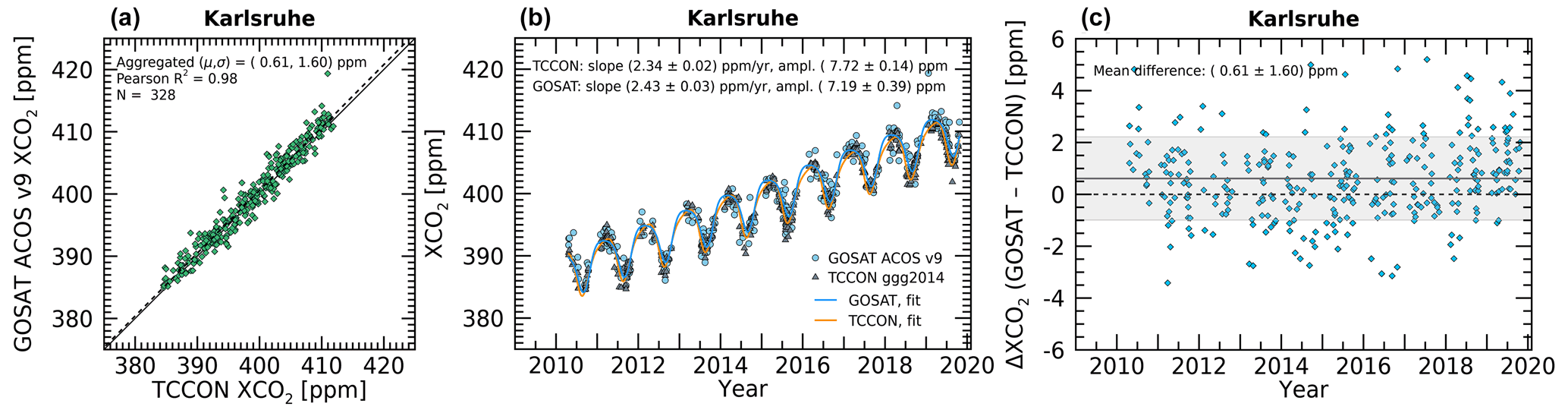
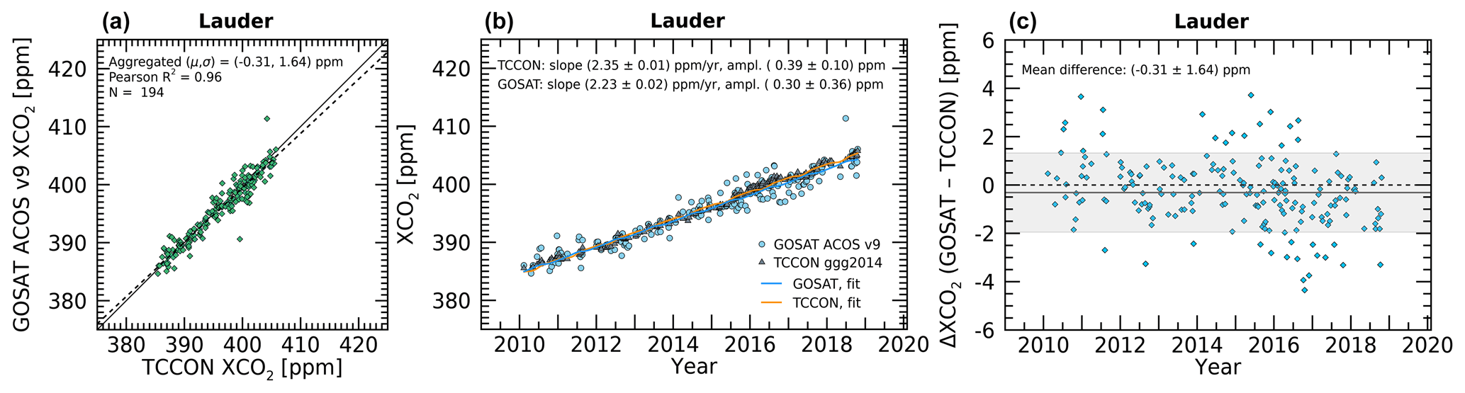
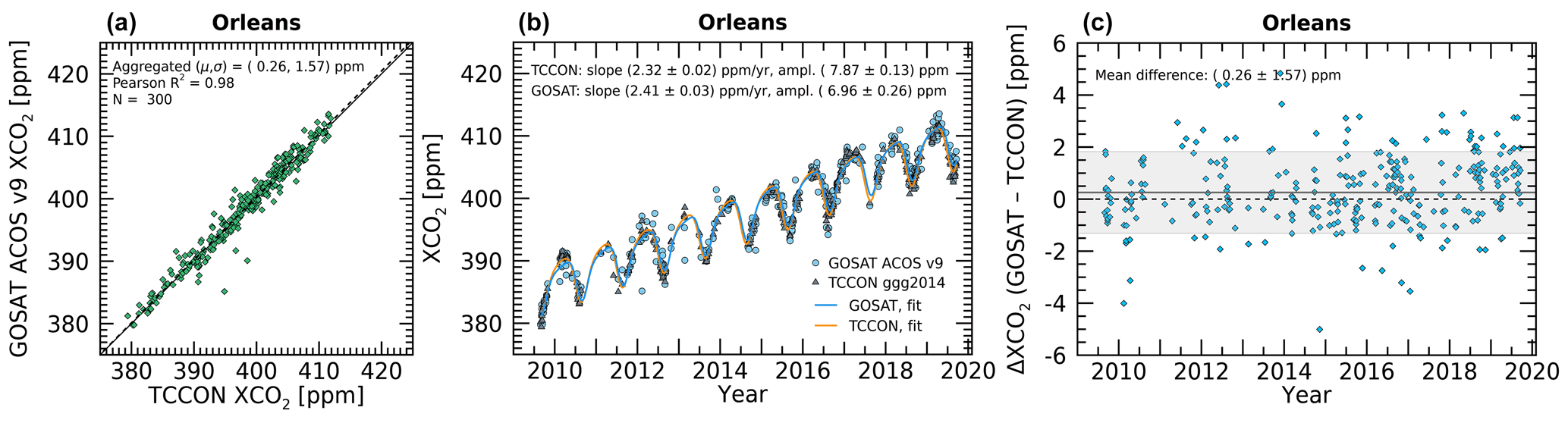
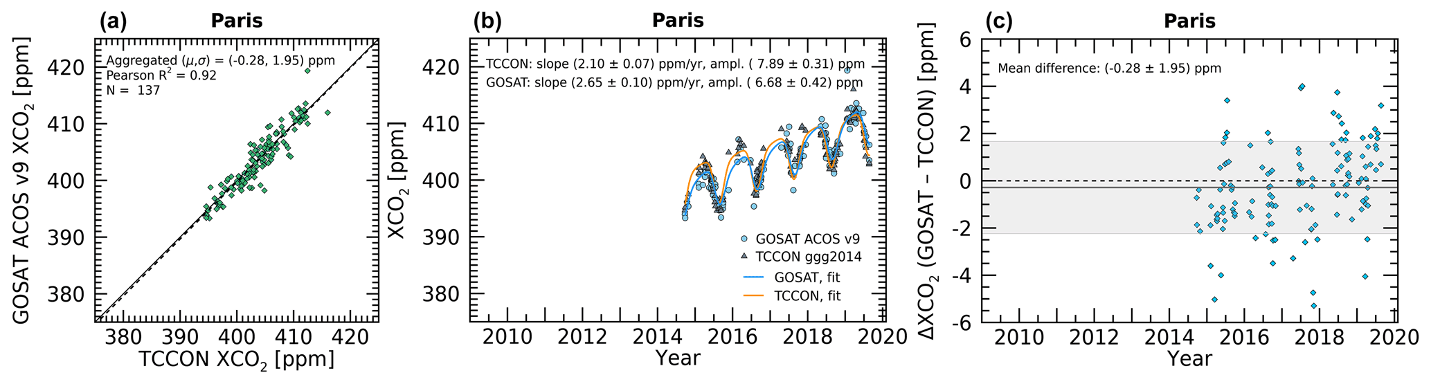
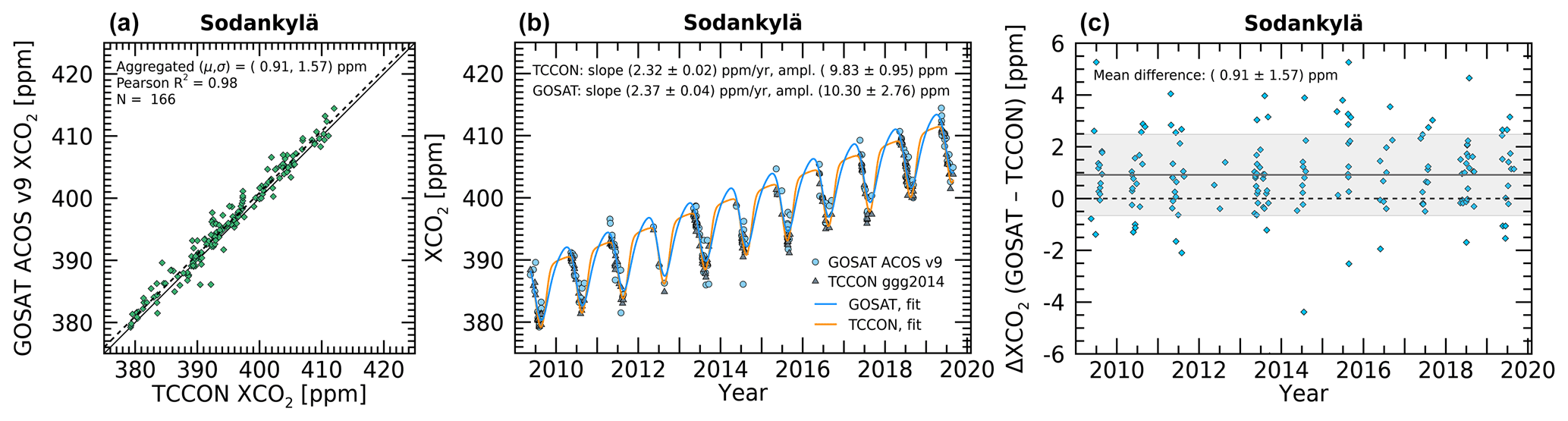
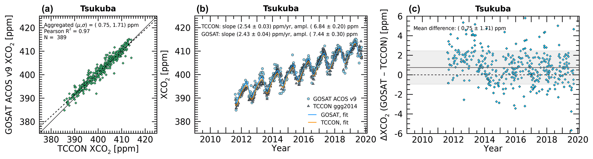
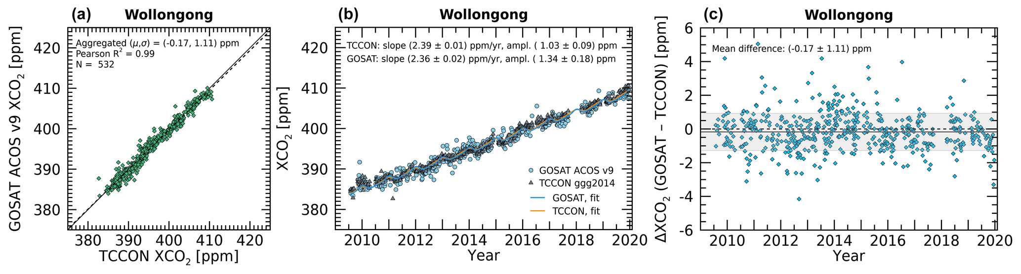
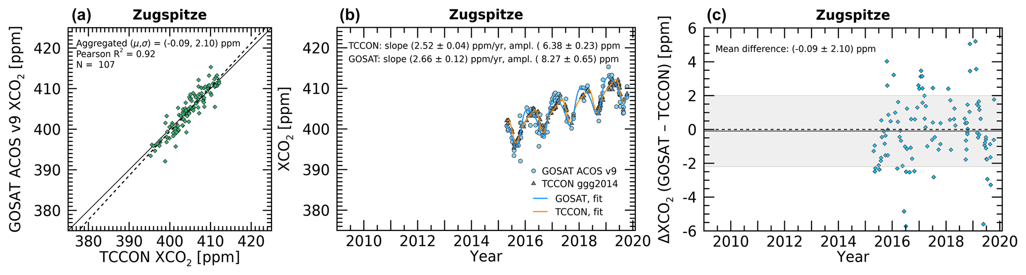
Knowledge of the average XCO₂ seasonal cycle can be used to disentangle the CO₂ growth rate from the seasonal variability, as well as for quantifying potential seasonal biases between satellite- and ground-based XCO₂ estimates. Lindqvist et al. (2015) fitted a skewed sine wave (see Eq. 1 of Lindqvist et al., 2015) to the ACOS GOSAT v3.5 XCO₂ time series and the TCCON estimates of XCO₂ at 16 stations, spanning April 2009 through December 2013. They found that ACOS GOSAT v7.3 captured the seasonal cycle within approximately 1 ppm of the TCCON estimates for all but the European sites and that the satellite- and ground-based CO₂ growth rates agreed generally better than 0.2 ppm per year. Here, we provide an update to those results using the 11-year ACOS GOSAT v9 XCO₂ data record. For this part of the analysis, a slightly more restrictive set of collocation criteria were implemented, compared to that described in Sect. 3.3 for the BC/QF procedure and to that used to generate Fig. 8. The seasonal cycle analysis required that the TCCON record spanned at least one contiguous year (a full seasonal cycle) and that a minimum of 20 collocations with GOSAT occurred. In addition, the three GOSAT observation modes (ocean H-gain, land M-gain, land H-gain) were combined for each site, and satellite overpass means of XCO₂ were aggregated into daily means. This resulted in approximately 7700 daily averages at 26 TCCON stations over the 11-year GOSAT data record.

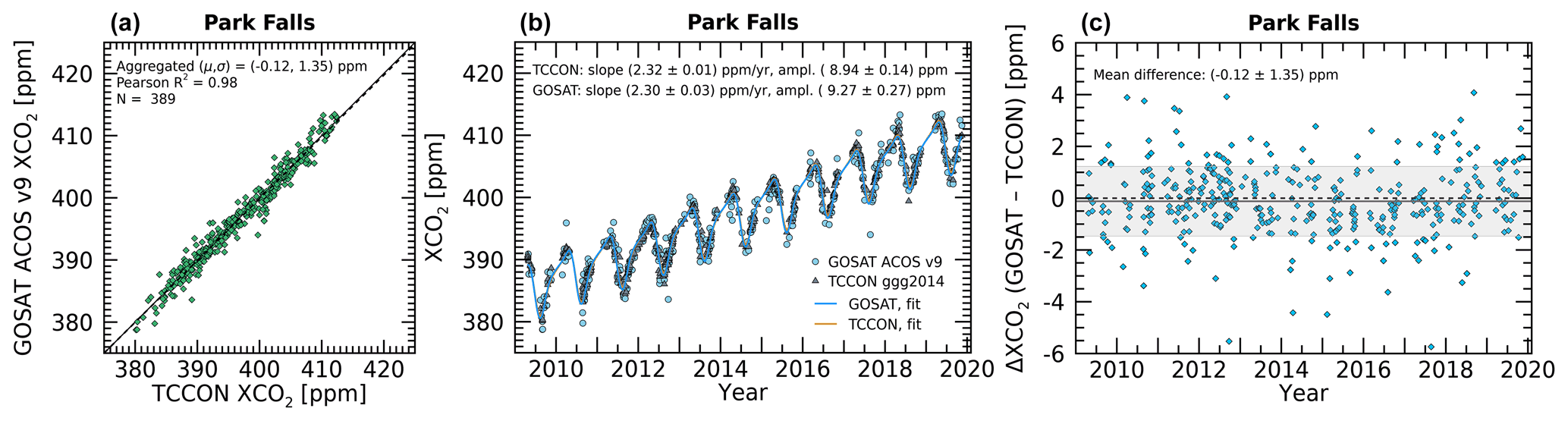
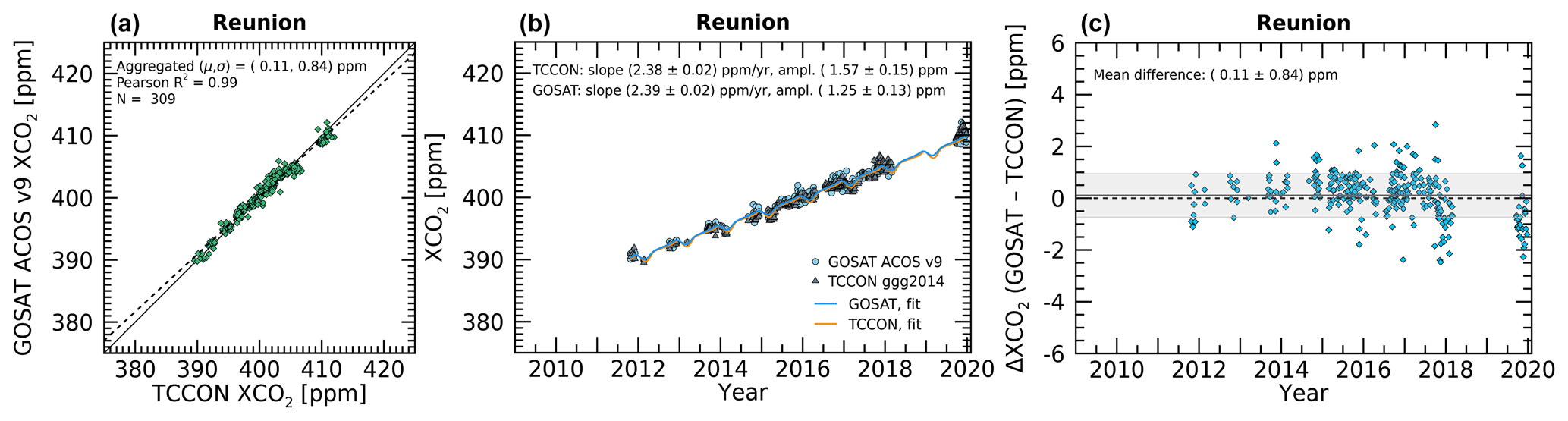
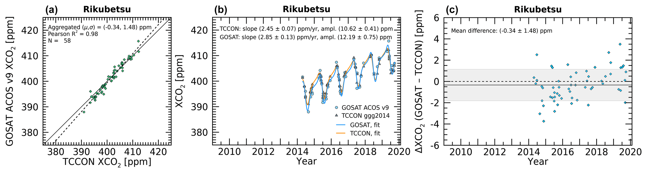
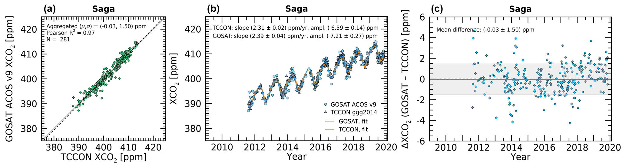
Figure 10 shows the results of the seasonal cycle fit for the Lamont, Oklahoma, TCCON station. The one-to-one scatter of the 896 daily averaged XCO₂ values (a) indicates a bias of −0.27 ppm for the GOSAT product relative to TCCON, with a standard deviation of 1.25 ppm and a Pearson's R² of 0.99. The seasonal cycle fits (b) indicate excellent agreement in the secular CO₂ increase at this site: 2.34 ppm for both GOSAT and TCCON. The mean seasonal amplitudes indicate a slight disagreement of a few tenths of a ppm, with TCCON showing a slightly higher fitted peak XCO₂ value during the spring maximum phase, compared to GOSAT. This is similar to the results for this site reported in Fig. 4 of Lindqvist et al. (2015). The time series of the calculated difference in satellite- and ground-based estimated XCO₂ (GOSAT − TCCON), shown in (c), highlights the magnitude of the scatter about the mean bias and suggests that there is no observable time drift in the data at this site.

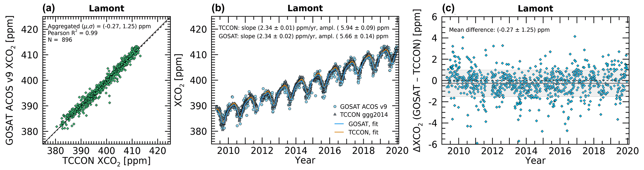
Figure 10 Seasonal cycle analysis of ACOS GOSAT v9 XCO₂ versus collocated TCCON for the Lamont, Oklahoma, station, following the methodology of Lindqvist et al. (2015). Panel (a) shows the one-to-one scatter plot of the bias-corrected daily mean XCO₂ for GOSAT versus TCCON. Panel (b) shows the time series of GOSAT XCO₂ (blue circles) with fit (blue line) and the TCCON XCO₂ (gray triangles) with fit (orange line) over the 11-year data record. Panel (c) shows the time series of calculated ΔXCO${}_{\mathrm{2}}^{\mathrm{TCCON}}$ (GOSAT – TCCON), with the mean difference (horizontal solid black line) and ±1 standard deviation (gray shading). The three GOSAT observation modes have been combined into daily mean averages to provide the maximum number of collocations possible for the seasonal fits.

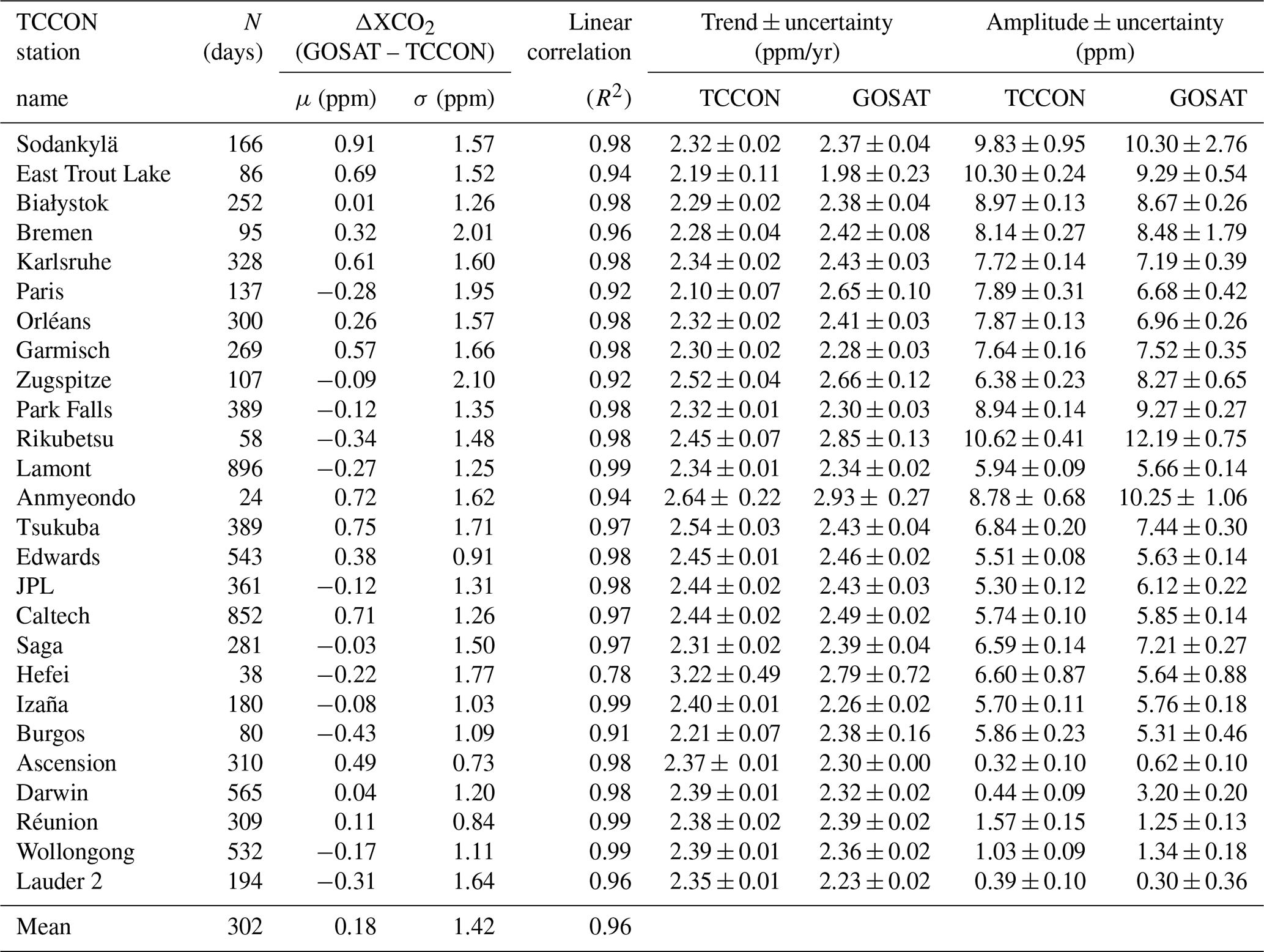
A summary of the data from each station that met the seasonal cycle collocation criteria is provided in Table 9. In addition, the full complement of plots is presented in Appendix A. Overall, the seasonal cycle analysis at most sites is in agreement, to within the estimated uncertainties. The standard deviation of the mean XCO₂ biases for the 26 sites is 0.41 ppm for the ACOS GOSAT v9 record. This compares to a value of 0.51 ppm at 23 stations for ACOS GOSAT v7.3, suggesting an improvement in the quality of the v9 XCO₂ product.

Table 9 Evaluation of the daily mean bias-corrected ACOS GOSAT v9 XCO₂ (all viewing modes combined) against collocated TCCON estimates for individual stations. There were 7741 d total for the 26 stations. The following sites/instruments were excluded from this part of the analysis due to inadequate time series or seasonal cycle coverage: Eureka, Four Corners, Indianapolis (Influx), JPL2007, Lauder1, Lauder3, Manaus, and Ny-Ålesund. The mean, standard deviation, and Pearson correlation coefficient (μ, σ, R²) of the linear fit between GOSAT and TCCON are given in columns 3–5. The remaining columns quantify the seasonal cycle fit following the methodology described in Lindqvist et al. (2015). The bottom row provides mean summary statistics for the linear fit.

4.4 ACOS GOSAT v9 XCO₂ versus models

The collocation and calculation of the multi-model-mean (MMM) is described in Sect. 3.3. Although the model data used for evaluation were very similar to those used in the QF/BC procedure, some minor version updates and extensions in time were included, as indicated in Table 4. It is important to be aware that there can be a considerable delay between performing the QF/BC procedure and the full generation of the final product, during which time the models are often updated.

Seasonal maps of ΔXCO${}_{\mathrm{2}}^{\mathrm{MMM}}$ (GOSAT v9 minus MMM) are shown in Fig. 11 for the 11-year data record binned at 2.5^∘ latitude by 5^∘ longitude. Generally, the agreement between the model-derived values and the satellite estimates is quite good, with an annual mean difference of $\simeq -\mathrm{0}$.15 ppm and binned scatter ≃ 0.5 ppm. For ocean H-gain observations, the ΔXCO${}_{\mathrm{2}}^{\mathrm{MMM}}$ tends to be negative (positive) in the Northern (Southern) Hemisphere. Land observations exhibit several distinct sub-continental-scale disagreements, including a strong positive signal over northern tropical Africa in DJF (GOSAT XCO₂ higher than MMM).

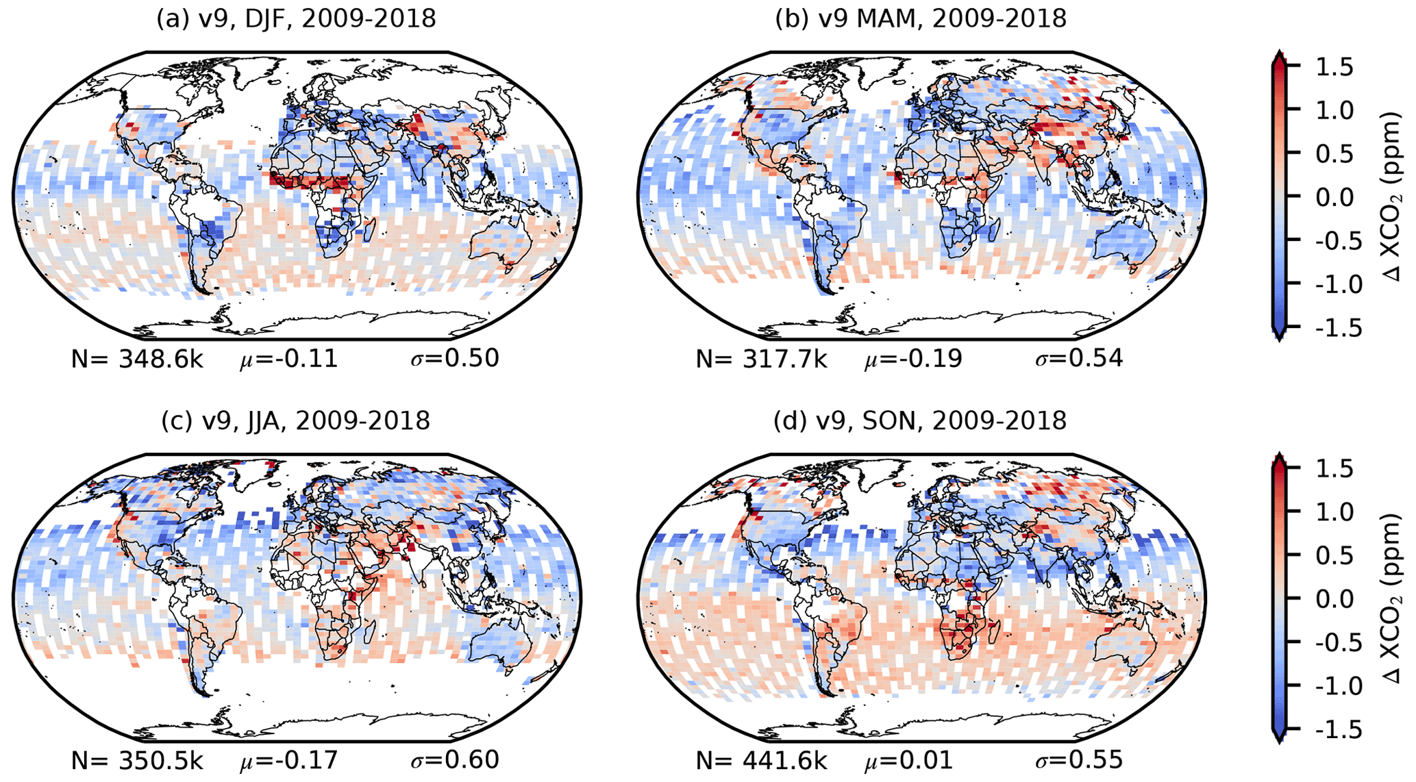
Figure 11 Seasonal maps of the mean ΔXCO${}_{\mathrm{2}}^{\mathrm{MMM}}$ (GOSAT – MMM) spanning 2009 through 2018 for DJF (a), MAM (b), JJA (c), and SON (d) at 2.5^∘ latitude by 5^∘ longitude resolution. Grid boxes containing fewer than 10 collocations are colored white.

Figure 12 shows Hovmöller plots of the ΔXCO${}_{\mathrm{2}}^{\mathrm{MMM}}$ ocean H-gain data at 30 d by 15^∘ latitude resolution for v7.3 (a) and v9 (a). The extension in time of v9 is evident, as well as the expansion in the latitude range of the ocean H-gain observations since 2015. A direct comparison between the v7.3 and v9 ΔXCO${}_{\mathrm{2}}^{\mathrm{MMM}}$ values for the overlapping time period, April 2009 through June 2016, reveals a global mean bias and standard deviation of −0.54 and 1.0 ppm for the v7.3 product, and −0.20 and 0.84 ppm for v9, underscoring the improvement.

Of particular note are the strong positive ΔXCO${}_{\mathrm{2}}^{\mathrm{MMM}}$ values in the v9 SH ocean H-gain observations for the latter part of 2014, persisting through most of 2015. This feature is not seen in the v7.3 product, due to a paucity of SH ocean H-gain data. It approximately coincides with the strong 2015–2016 El Ninõ event, where ΔXCO${}_{\mathrm{2}}^{\mathrm{MMM}}$ signals were also seen in the OCO-2 v7 ocean H-gain data, as reported in Chatterjee et al. (2017). It has been hypothesized that the 2015–2016 El Ninõ produced an anomalously strong carbon release from tropical land regions due to higher temperature and below average precipitation (Liu et al., 2017). In contrast to the positive SH signal, negative ΔXCO${}_{\mathrm{2}}^{\mathrm{MMM}}$ values (GOSAT lower than MMM) have been observed in the v9 NH oceans since 2016. It is unclear why the satellite and models disagree over such large spatial and temporal scales, but recent work by Müller et al. (2021) suggests that the ACOS v7.3 (and to a lesser extent v9) XCO₂ values are in fact biased low by approximately 1 to 1.5 ppm, as compared to a new independent evaluation data set generated from combined ship and aircraft measurements over the open oceans. Further investigation into the source of the ACOS GOSAT biases against models is warranted.

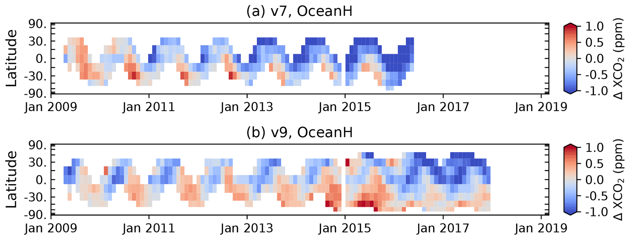
Figure 12 Time series of ΔXCO${}_{\mathrm{2}}^{\mathrm{MMM}}$ (ACOS GOSAT v9 – MMM) versus latitude at 30 d by 15^∘ resolution for ocean H-gain observations for v7.3 (a) and v9 (b). Grid cells containing fewer than 10 collocations are colored white.

Figure 13 shows spatial maps of ΔXCO${}_{\mathrm{2}}^{\mathrm{MMM}}$ for the truncated time span 2010 through 2015 comparing v7.3 (a and c) and v9 (b and d) for DJF (a and b) and JJA (c and d). There is significant decrease in scatter in the v9 product (≃ 0.5 ppm) relative to v7.3 (≃ 0.75 ppm). The low bias in DJF tropical Pacific vanishes in v9, and the positive bias in JJA extratropical land regions is reduced. The expanded latitudinal extent of the ocean H-gain observations is evident in the v9 maps. One feature that is robust in both v7.3 and v9 is the large positive signal over northern tropical Africa in DJF. This feature was also observed in the OCO-2 v7 and v8 comparisons to a MMM (O'Dell et al., 2018) and in v10 XCO₂ anomaly maps (Hakkarainen et al., 2019).

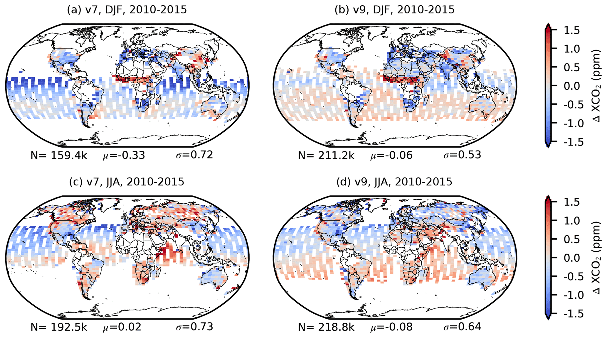
Figure 13 Maps of the mean ΔXCO${}_{\mathrm{2}}^{\mathrm{MMM}}$ (GOSAT – MMM) spanning 2010 through 2015 for v7.3 DJF (a), v9 DJF (b), v7.3 JJA (c), and v9 JJA (d) at 2.5^∘ by 5^∘ latitude–longitude resolution. Only grid boxes with at least 10 collocations are shown.

4.5 ACOS GOSAT v9 XCO₂ versus OCO-2

NASA's Orbiting Carbon Observatory-2 (OCO-2) has been collecting science data since September, 2014 from a near-polar low-Earth orbit (705 km altitude), with an afternoon Equator crossing time of ≃ 13:30 local time (Crisp et al., 2017). Like GOSAT, OCO-2 takes measurements of reflected solar radiation in the oxygen A-band (0.76 µm) and the weak and strong carbon dioxide bands (1.6 and 2.0  µm, respectively), which are used to estimate XCO₂ using the ACOS L2FP retrieval algorithm (Eldering et al., 2017; O'Dell et al., 2018). However, due to differences in the orbit parameters of the two sensors, e.g., a 3 d repeat cycle for GOSAT versus a 16 d repeat cycle for OCO-2 (see Table 2 of Kataoka et al., 2017), the number of collocated soundings is somewhat limited. Therefore, some criteria must be defined in order to identify soundings that can be compared in a meaningful way. The underlying assumption of the collocation is that on scales of a few hundred kilometers and several hours, the natural variance in XCO₂ is not detectable in satellite-derived estimates from the ACOS L2FP algorithm.

For this study, the coincidence criteria to match OCO-2 soundings to individual GOSAT soundings were as follows: (i) falling within 2^∘ latitude and 3^∘ longitude, (ii) with a maximum spatial separation of 300 km, and (iii) acquired within ±2 h. Due to the dense nature of the OCO-2 soundings relative to the sparseness of the GOSAT soundings, there are typically between zero and several hundred matched OCO-2 soundings per GOSAT footprint. A lower limit of 10 and an upper limit of 100 (randomly selected) OCO-2 soundings that meet the coincidence criteria were set in order to retain the GOSAT sounding for analysis. The individual L2FP quality flags are applied for both GOSAT and OCO-2 during the collocation procedure, and then the mean value of XCO₂ from the 10 to 100 collocated OCO-2 soundings is calculated and subtracted from the corresponding GOSAT XCO₂ to produce ΔXCO${}_{\mathrm{2}}^{\mathrm{OCO}-\mathrm{2}}$.

Here we compare ACOS GOSAT v9 against OCO-2 v10 (rather than to the deprecated v9), since we assume that science users will adopt the newest OCO-2 product. Major updates to the version 10 ACOS L2FP algorithm (Osterman et al., 2020) are discussed in Sect. 3.1.

One complexity in comparing ACOS GOSAT v9 and OCO-2 v10 is the fact that the two versions of the algorithm used different CO₂ priors. Typically, models which assimilate satellite CO₂ data take into account the unmeasured part of the prior CO₂ profile (specified via the retrieval's averaging kernel) via an averaging kernel correction, as given in Eq. (1). Therefore, in order to fairly compare these two data sets as models would assimilate them, we need to remove their difference due to the unmeasured part of the CO₂ profile, as follows:

$$\begin{array}{}\text{(3)}& {\mathrm{XCO}}_{\mathrm{2}}^{\prime }={\mathrm{XCO}}_{\mathrm{2}}+\sum _{i=\mathrm{1}}^{\mathrm{20}}{h}_i(\mathrm{1}-a_i)\cdot (u_{\mathrm{a},i}^{\prime }-u_{\mathrm{a},i}),\end{array}$$

where h is the XCO₂ pressure weighting function, a is the normalized XCO₂ averaging kernel, u_a is the ACOS v9 CO₂ prior profile used for GOSAT, and $u_{\mathrm{a}}^{\prime }$ is the ACOS v10 CO₂ prior profile used for OCO-2. The summation takes place over the 20 vertical levels defined in the ACOS code. In summary, the total adjustment to the ACOS GOSAT XCO₂ value is calculated as the contribution of the difference in the vertical CO₂ priors at each level weighted by the one minus the averaging kernel at that level. The global mean adjustment due to the CO₂ prior correction was approximately 0.2 ppm, with 95 % of corrections between −0.1 and +0.5 ppm.

Spatial maps of ΔXCO${}_{\mathrm{2}}^{\mathrm{OCO}-\mathrm{2}}$ (GOSAT v9 – OCO-2 v10) for the prior-corrected, collocated soundings are shown in Figs. 14 and 15 for land and ocean, respectively. In each figure the maps are shown by season at 2.5^∘ latitude by 5^∘ longitude resolution. In all seasons, higher scatter in ΔXCO${}_{\mathrm{2}}^{\mathrm{OCO}-\mathrm{2}}$ is observed over land (≃1 ppm) than over ocean (< 0.7 ppm), likely due to variability of land surface features and/or lower signal-to-noise ratios of the radiance measurements. The annual global mean ΔXCO${}_{\mathrm{2}}^{\mathrm{OCO}-\mathrm{2}}$ for land is near zero (0.06 ppm) and exhibits little variation with season. For ocean H-gain, the global mean ΔXCO${}_{\mathrm{2}}^{\mathrm{OCO}-\mathrm{2}}$ is larger (−0.40 ppm) and varies more significantly by season from −0.2 (DJF) to −0.6 ppm (JJA). The disagreements in the ocean H-gain data tend to be spatially coherent, with a notably large negative difference in the NH in most seasons. Currently, the underlying cause of these disagreements is unknown and could stem from instrument calibration or sampling-related issues, differences in retrieval algorithm versions, or even collocation issues.

Figure 14 Spatial distribution of the bias-corrected ΔXCO${}_{\mathrm{2}}^{\mathrm{OCO}-\mathrm{2}}$ (GOSAT v9 minus OCO-2 v10) for the good QF land soundings for DJF (a), MAM (b), JJA (c), and SON (D) for the overlapping period August 2014 through June 2020. The spatiotemporal requirements for matched soundings are a maximum separation of 300 km, and observation time within ±2 h. Maps are gridded at 2.5^∘ latitude by 5^∘ longitude resolution, and only grid boxes with at least 10 matched soundings are shown.

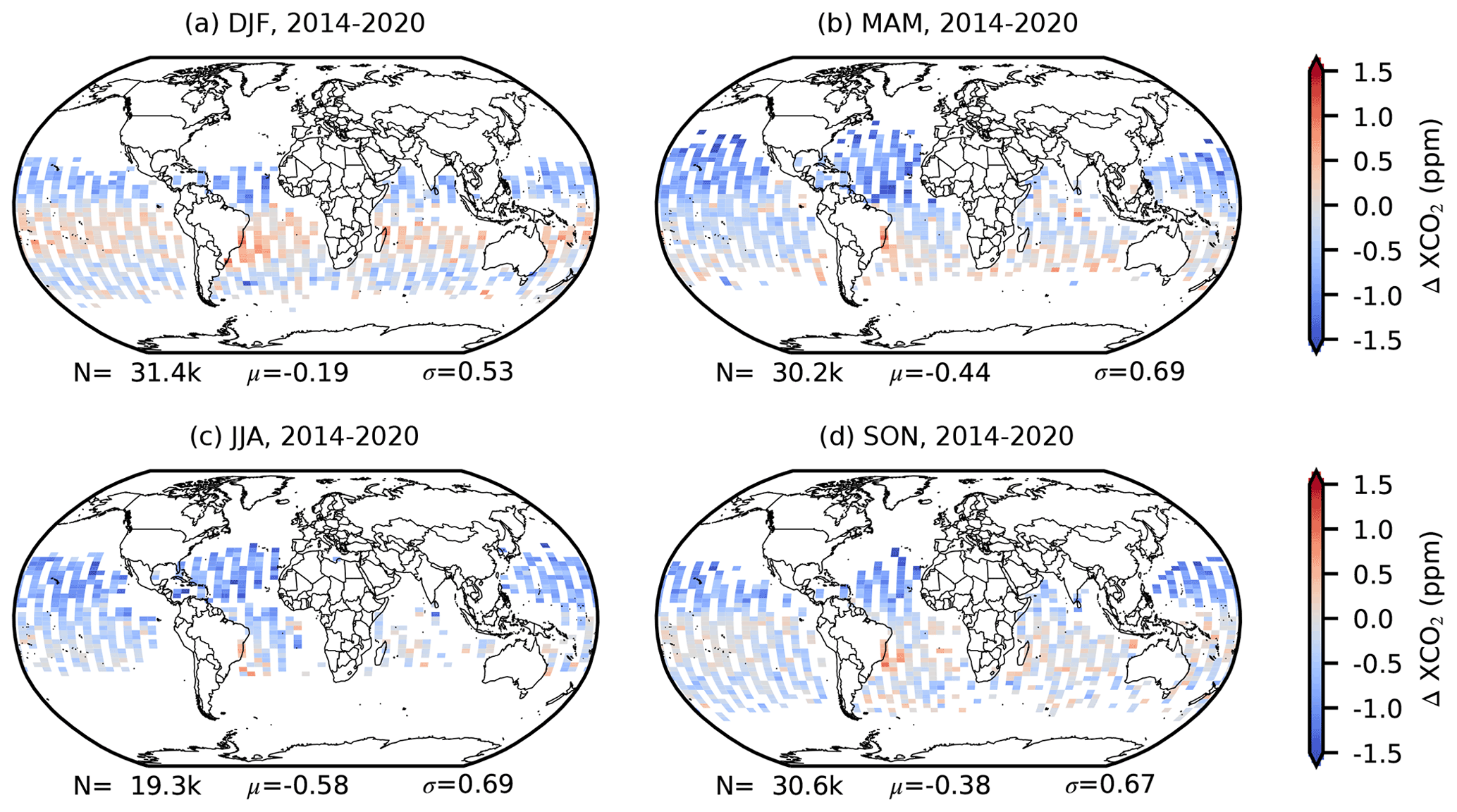
Figure 15 Same as Fig. 14, but for ocean H-gain observations.

The disagreement in XCO₂ for ocean H-gain between ACOS GOSAT v9 and OCO-2 v10 is highlighted in panel (a) of Fig. 16, which shows ΔXCO${}_{\mathrm{2}}^{\mathrm{OCO}-\mathrm{2}}$ for the period September 2014 through December 2020 at 30 d by 15^∘ latitude resolution for the ocean H-gain observations. Panel B shows the number of collocated soundings in each bin. A large SH positive difference in ΔXCO${}_{\mathrm{2}}^{\mathrm{OCO}-\mathrm{2}}$ (GOSAT higher than OCO-2 by ≃ 0.5 ppm) is observed for the first 2 years of the time record. Then, in early 2016, there is what appears to be an abrupt jump to a large negative difference (GOSAT lower than OCO-2 by $\simeq -$0.5 ppm) in the NH. From this point forward, ΔXCO${}_{\mathrm{2}}^{\mathrm{OCO}-\mathrm{2}}$ appears to be reasonably stable in time, although there is a persistent low difference in the NH for the remainder of the record.

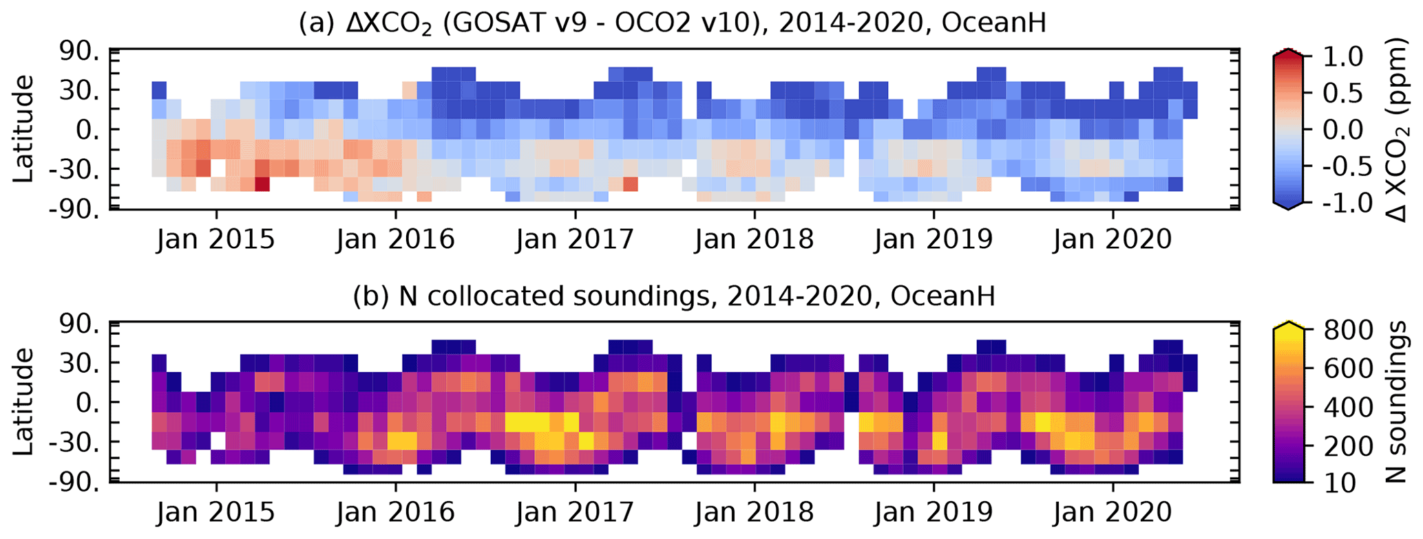
Figure 16 Difference in XCO₂ between ACOS GOSAT v9 and OCO-2 v10 (ΔXCO${}_{\mathrm{2}}^{\mathrm{OCO}-\mathrm{2}}$) as a function of time and latitude at 30 d by 15^∘ latitude resolution for ocean H-gain observations (a). Panel (b) shows the sounding density of the collocated soundings. Grid cells containing fewer than 10 collocations are colored white.

Figure 17 shows the ΔXCO${}_{\mathrm{2}}^{\mathrm{OCO}-\mathrm{2}}$ data for the combined land H-gain and M-gain data, similar to Fig. 16. The main feature here is that the overall variability is larger compared to the ocean H-gain data, which we attribute to biases introduced by variations in both topography and surface albedo. A slightly positive (red) signal is observed during the September to December months in the SH, especially in 2014, 2018, and 2019. Although additional investigation into such signals is warranted, it is beyond the scope of the current work.

Figure 17 Same as Fig. 16, but for land observations (combined H-gain and M-gain).

A set of summary statistics for the ACOS GOSAT v9 versus OCO-2 v10 XCO₂ product is given in Table 10. The values reported here are on the individual collocations by year and season, rather than the spatially gridded averages as given in Figs. 14 and 15. For the land observations, there has been a very slight upward trend in time of the ΔXCO${}_{\mathrm{2}}^{\mathrm{OCO}-\mathrm{2}}$ to slightly more positive values (GOSAT v9 larger than OCO-2 v10 XCO₂). On the other hand, for ocean H-gain observations, the general trend has been an increasingly more negative ΔXCO${}_{\mathrm{2}}^{\mathrm{OCO}-\mathrm{2}}$ in time, as is seen in Fig. 16. Additional investigation will be required to determine the root cause(s) of these differences.

Table 10 A set of summary statistics for the comparison of the ACOS GOSAT v9 XCO₂ to the OCO-2 v10 product. Individual collocations for each year and season are given by N, while the mean ΔXCO₂ and the standard deviation from the mean are given by μ and σ, respectively, both in units ppm. The top portion of the table is for land observations, while the bottom is for ocean H-gain (OceanH).

5 Data availability

The ACOS GOSAT v9 XCO₂ data are available on the NASA Goddard Earth Science Data and Information Services Center (GES-DISC) in both the per-orbit full format (OCO-2 Science Team et al., 2019b, https://doi.org/10.5067/OSGTIL9OV0PN) and in the per-day lite format (OCO-2 Science Team et al., 2019a, https://doi.org/10.5067/VWSABTO7ZII4). The monthly super-lite files, containing only the most essential variables for each satellite observation, are available at CaltechDATA (https://doi.org/10.22002/D1.2178, Eldering, 2021). The OCO-2 v10 L2Lite files containing the bias-corrected and quality-filtered XCO₂ data are also available on the GES-DISC (OCO-2 Science Team et al., 2020, https://doi.org/10.5067/E4E140XDMPO2). The TCCON data for individual stations are available on the CaltechDATA site (see citations listed in Table 8). The CarbonTracker data are available on the NOAA GML site (https://carbontracker.noaa.gov, CarbonTracker, 2021). The CarboScope model data are available at http://www.bgc-jena.mpg.de/CarboScope (CarboScope, 2021). The CAMS model data are available at https://atmosphere.copernicus.eu/data (CAMS, 2021). The UoL model data are available at https://www.geos.ed.ac.uk/~lfeng/ (UoE, 2021).

6 Summary

The v9 ACOS GOSAT XCO₂ product, spanning February 2009 through June 2020, has been compared to XCO₂ estimates from TCCON, a suite of atmospheric inversion systems (models), and with collocated OCO-2 v10 data. The ACOS GOSAT v9 product is an improvement over ACOS GOSAT v7.3 relative to these standards. The v9 product provides a significant extension of the data record and contains data in M-gain viewing mode over bright land surfaces.

Of the 37.4×10⁶ estimates of XCO₂ contained in the ACOS GOSAT v9 data record, approximately 80 % were prefiltered due to contamination by cloud and/or aerosol, or due to insufficient SNR. Of the 7.0×10⁶ that were selected to run through the ACOS L2FP algorithm, approximately 6.1×10⁶ returned valid estimates of XCO₂. However, only ≃ 2×10⁶ of those were identified as being of “good” quality. This represents 5.4 % of the total recorded soundings. The quality filtering and bias correction variables used for ACOS GOSAT v9 were similar to those used in previous product versions, and similar to those used for OCO-2 v9 and v10, but include for the first time, a correction to account for a small temporal drift in the data.

Comparisons with collocated estimates of XCO₂ from TCCON indicate overpass mean biases of ≃ 0.1 to 0.2 ppm and standard deviations of ≃ 1.5 ppm. The mean squared error against TCCON is highest for land observations in the northern mid-latitudes (30–60^∘ N), and lowest for ocean H-gain and SH land M-gain observations. The statistics show improvement when compared to the results for v7.3, which spanned a shorter time period (April 2009 to June 2016). Specifically, the standard deviation of the mean station bias for the 26 sites is 0.41 ppm for the ACOS GOSAT v9 record, compared to 0.51 ppm at 23 stations for ACOS GOSAT v7.3.

Comparisons with collocated XCO₂ derived from a suite of four atmospheric inversion systems (models) suggest annual global mean differences of ≃ 0.15 ppm and standard deviation of ≃ 0.5 ppm. Hemispherical differences in XCO₂ estimates over oceans were observed, as well as robust subcontinental-scale land features. Results indicate better agreement with models in the ACOS v9 product ($\mathit{\mu }=-\mathrm{0}$.20 ppm, σ=0.8 ppm) compared to v7.3 ($\mathit{\mu }=-\mathrm{0}$.54 ppm, σ=1.0 ppm) for the overlapping period April 2009 through June 2016, but further investigation is required to explain the remaining disagreement over large spatial and temporal scales.

Comparisons with collocated OCO-2 v10 XCO₂ data show low bias but relatively high scatter for land observations (μ=0.06 ppm, σ=1.0 ppm, when averaged across seasons). Increased scatter over land is expected due to XCO₂ bias introduced by variability in topography and surface albedo. However, for ocean H-gain observations, although the XCO₂ scatter is lower than that for land as expected (σ=0.7 ppm), the global mean bias is relatively high ($\mathit{\mu }=-\mathrm{0}$.4 ppm, when averaged across seasons). These are issues that must be resolved in order for GOSAT v9 and OCO-2 v10 data to provide consistent information to atmospheric inversion systems for assessing fluxes of CO₂.

Global estimates of CO₂ derived from satellite measurements provide coverage in traditionally data-sparse regions where ground-based measurements are difficult. The assimilation of satellite XCO₂ into atmospheric inversion systems to quantify the spatiotemporal variations of carbon fluxes is a promising, but challenging, area of research. This research continues to benefit from various improvements in transport models, atmospheric inversion systems, and satellite retrievals. The role of the GOSAT record in this field remains unique due to its exceptional 11-year length and its coverage of nearly 5.5 years of the carbon cycle prior to the launch of OCO-2. The ACOS GOSAT v9 L2Std and L2Lite file products are both available on the NASA GES DISC (OCO-2 Science Team et al., 2019b, a).

Appendix A: Seasonal cycle plots of ACOS GOSAT v9 XCO₂ versus TCCON for individual stations

Figure A1 Daily averaged bias-corrected ACOS GOSAT v9 versus collocated TCCON XCO₂ at Anmyeondo, South Korea. Left panel (a) shows the one-to-one scatter plot of the daily mean XCO₂ for GOSAT versus TCCON. Middle panel (b) shows the time series of daily mean GOSAT XCO₂ (blue circles) with fit (blue line) and the TCCON XCO₂ (gray triangles) with fit (orange line) over the 11-year data record. Right panel (c) shows the time series of calculated ΔXCO${}_{\mathrm{2}}^{\mathrm{TCCON}}$, with the mean difference (horizontal solid black line) and ±1 standard deviation (gray shading). In these plots, the three GOSAT observation modes have been combined in order to provide the maximum number of collocations possible for the seasonal fits.

Figure A2 Same as Fig. A1, but for Ascension Island, located in the Pacific Ocean off the west coast of Africa.

Figure A3 Same as Fig. A1, but for Białystok, Poland.

Figure A4 Same as Fig. A1, but for Bremen, Germany.

Figure A5 Same as Fig. A1, but for Burgos, Philippines.

Figure A6 Same as Fig. A1, but for Caltech, California.

Figure A7 Same as Fig. A1, but for Darwin, Australia.

Figure A8 Same as Fig. A1, but for Edwards, California.

Figure A9 Same as Fig. A1, but for East Trout Lake, Canada.

Figure A10 Same as Fig. A1, but for Garmisch, Germany.

Figure A11 Same as Fig. A1, but for Hefei, China.

Figure A12 Same as Fig. A1, but for Izaña, Tenerife, Spain.

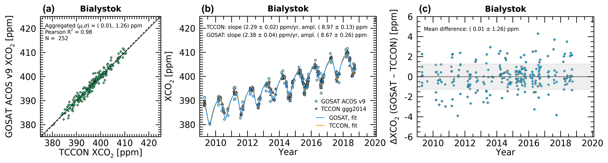
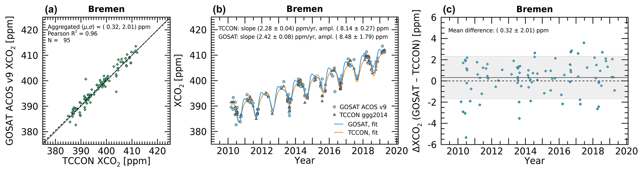
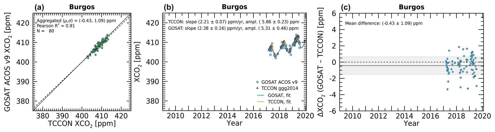
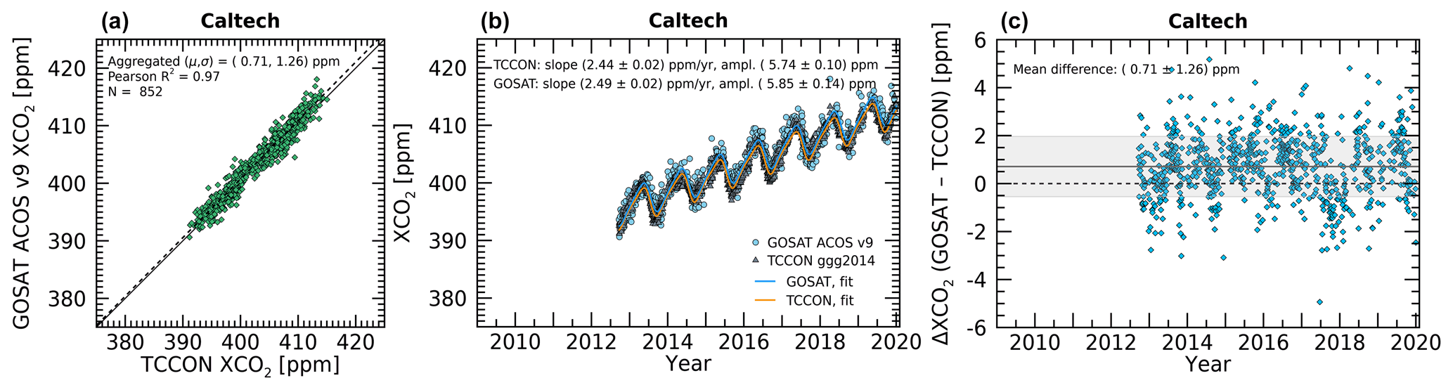
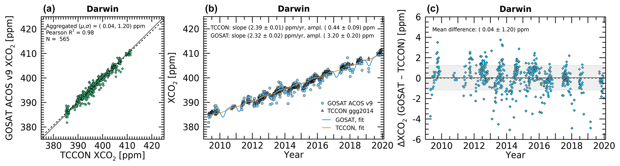
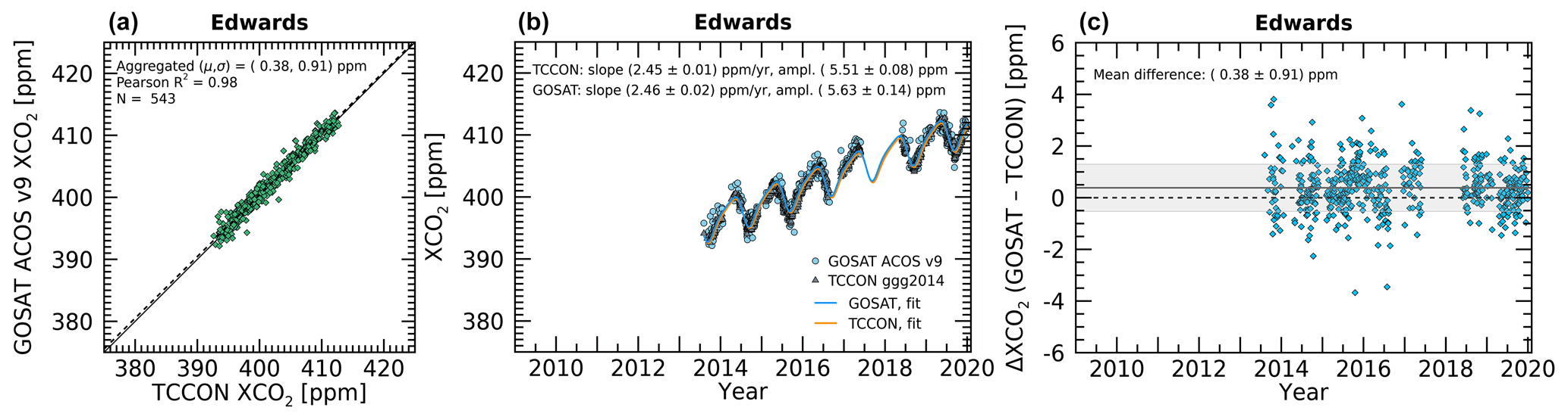
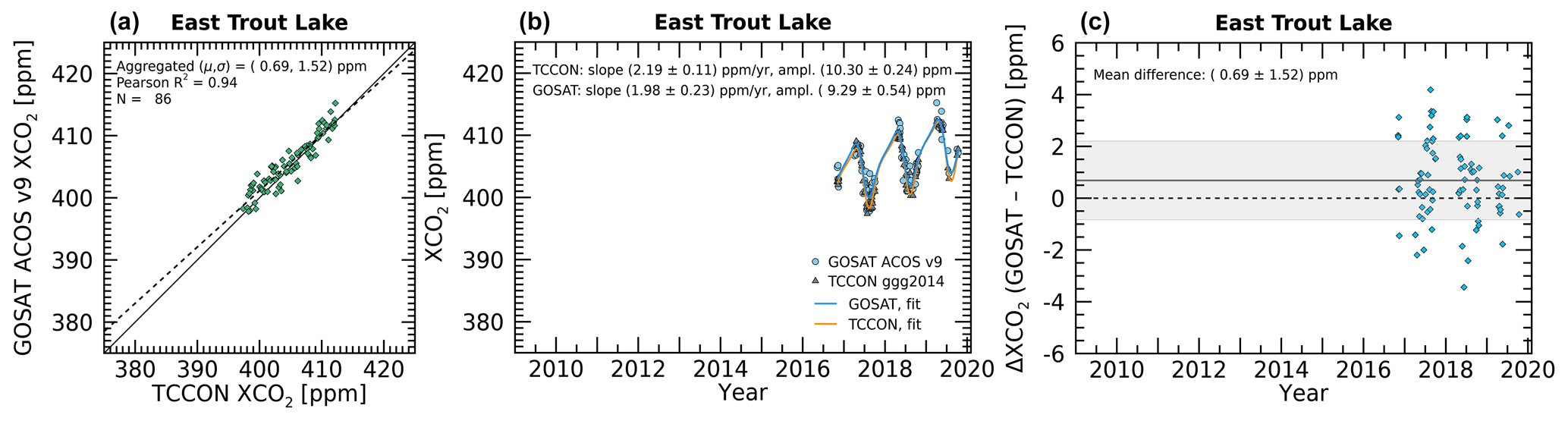
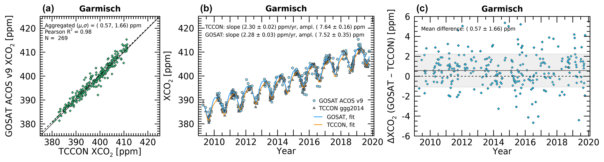
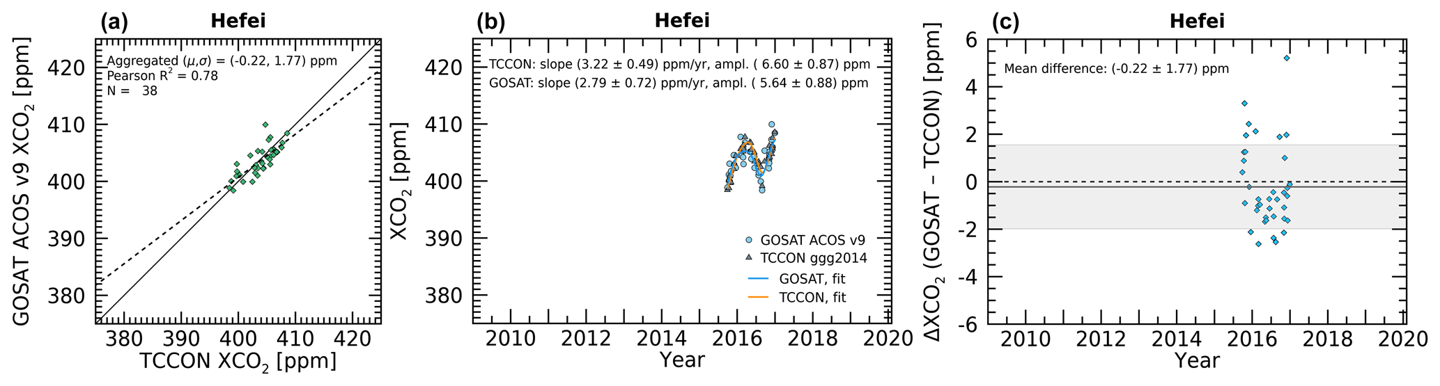
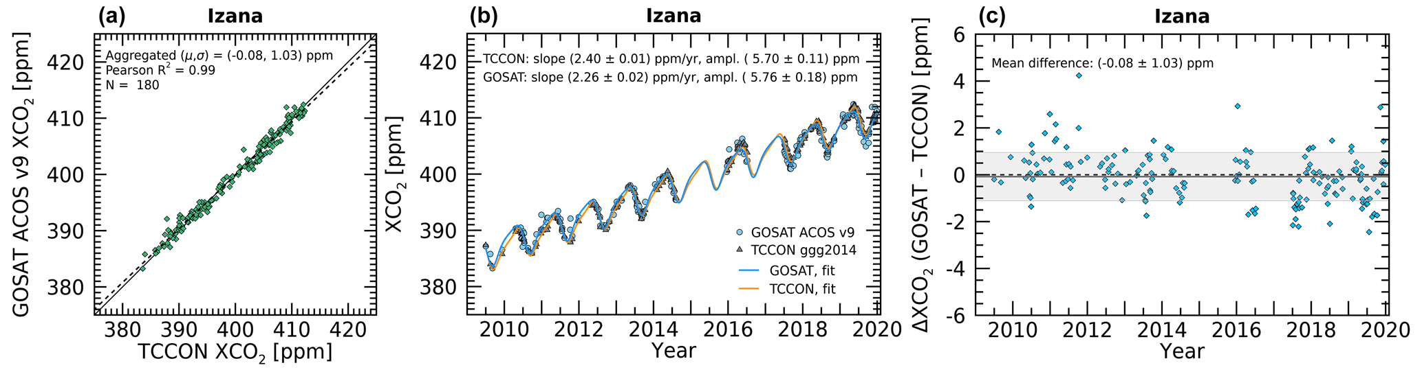
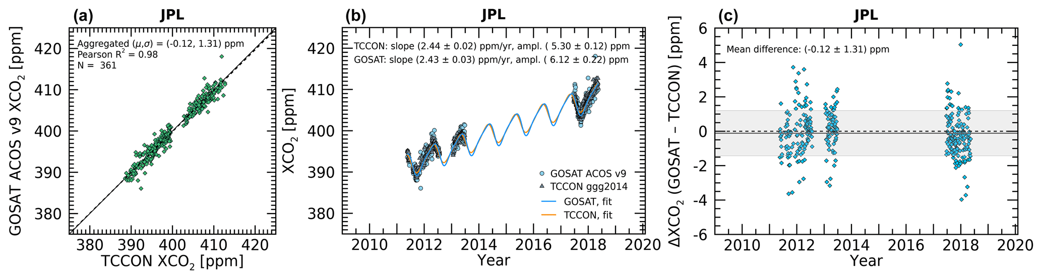
Figure A13 Same as Fig. A1, but for Jet Propulsion Laboratory (JPL), Pasadena, California. This site has been used occasionally for the simultaneous operation of a TCCON instrument during the thermal vacuum testing of OCO-2 (Frankenberg et al., 2015) and OCO-3.

Figure A14 Same as Fig. A1, but for Karlsruhe, Germany.

Figure A15 Same as Fig. A1, but for Lauder, New Zealand.

Figure A16 Same as Fig. A1, but for Orléans, France.

Figure A17 Same as Fig. A1, but for Paris, France.

Figure A18 Same as Fig. A1, but for Park Falls, Wisconsin.

Figure A19 Same as Fig. A1, but for Réunion, off the east coast of Madagascar.

Figure A20 Same as Fig. A1, but for Rikubetsu, Japan.

Figure A21 Same as Fig. A1, but for Saga, Japan.

Figure A22 Same as Fig. A1, but for Sodankylä, Finland.

Figure A23 Same as Fig. A1, but for Tsukuba, Japan.

Figure A24 Same as Fig. A1, but for Wollongong, Australia.

Figure A25 Same as Fig. A1, but for Zugspitze, Germany.