A global dataset of spatiotemporally seamless daily mean land surface temperatures: generation, validation, and analysis

Daily mean land surface temperatures (LSTs) acquired from polar orbiters are crucial for various applications such as global and regional climate change analysis. However, thermal sensors from polar orbiters can only sample the surface effectively with very limited times per day under cloud-free conditions. These limitations have produced a systematic sampling bias (ΔT_sb) on the daily mean LST (T_dm) estimated with the traditional method, which uses the averages of clear-sky LST observations directly as the T_dm. Several methods have been proposed for the estimation of the T_dm, yet they are becoming less capable of generating spatiotemporally seamless T_dm across the globe. Based on MODIS and reanalysis data, here we propose an improved annual and diurnal temperature cycle-based framework (termed the IADTC framework) to generate global spatiotemporally seamless T_dm products ranging from 2003 to 2019 (named the GADTC products). The validations show that the IADTC framework reduces the systematic ΔT_sb significantly. When validated only with in situ data, the assessments show that the mean absolute errors (MAEs) of the IADTC framework are 1.4 and 1.1 K for SURFRAD and FLUXNET data, respectively, and the mean biases are both close to zero. Direct comparisons between the GADTC products and in situ measurements indicate that the MAEs are 2.2 and 3.1 K for the SURFRAD and FLUXNET datasets, respectively, and the mean biases are −1.6 and −1.5 K for these two datasets, respectively. By taking the GADTC products as references, further analysis reveals that the T_dm estimated with the traditional averaging method yields a positive systematic ΔT_sb of greater than 2.0 K in low-latitude and midlatitude regions while of a relatively small value in high-latitude regions. Although the global-mean LST trend (2003 to 2019) calculated with the traditional method and the IADTC framework is relatively close (both between 0.025 to 0.029 K yr⁻¹), regional discrepancies in LST trend do occur – the pixel-based MAE in LST trend between these two methods reaches 0.012 K yr⁻¹. We consider the IADTC framework can guide the further optimization of T_dm estimation across the globe, and the generated GADTC products should be valuable in various applications such as global and regional warming analysis. The GADTC products are freely available at https://doi.org/10.5281/zenodo.6287052 (Hong et al., 2022).

1 Introduction

Land surface temperature (LST) is one of the most important variables of land–atmosphere interaction (Jin and Dickinson, 2010). Currently, satellite thermal remote sensing provides the only way to obtain long-term and regular LST over extensive areas. The archived long-term satellite-derived LST datasets have been widely used in various fields such as land cover change detection (Lambin and Ehrlich, 1997; Muro et al., 2018), radiation flux simulation (Alcântara et al., 2010; Anderson et al., 2007), drought monitoring (Karnieli et al., 2010; Mildrexler et al., 2017), vegetation change analysis (Julien and Sobrino, 2009; Julien et al., 2006; Still et al., 2019), permafrost thawing monitoring (Westermann et al., 2011), and global LST trend investigation (Jin, 2004; Jin and Dickinson, 2002; Yan et al., 2020).

According to the satellite onboard duration and spatiotemporal resolution (Tomlinson et al., 2011), satellite-derived LST products used for long-term time-series analysis can be divided into two categories: (1) the LSTs obtained from high-orbit geostationary satellite sensors with a coarse spatial resolution (3–5 km), e.g., the MSG-SEVIRI (the Spinning Enhanced Visible and Infrared Imager onboard Meteosat Second Generation) and GOES (Geostationary Operational Environmental Satellite), and (2) the LSTs from low-orbit polar-orbiting satellite sensors. The second category of satellite sensors can be further divided into (1) the narrow-swath polar-orbiting satellite sensors with a relatively high spatial resolution (around 100 m), e.g., Landsat and ASTER (Advanced Spaceborne Thermal Emission and Reflection Radiometer) and (2) the polar-orbiting satellite sensors with a moderate spatial resolution (around 1 km), e.g., AVHRR (Advanced Very High-Resolution Radiometer), SLSTR (Sea and Land Surface Temperature Radiometer), and MODIS (Moderate Resolution Imaging Spectroradiometer).

The geostationary satellite thermal sensors are characterized by a very high temporal resolution (1 h or finer). However, they are relatively difficult to provide global consistent LST products due to the limited coverage of a single geostationary satellite and the systematic errors among different satellites (Freitas et al., 2013). The Landsat (or similar polar orbiters) has been providing thermal observations since the 1980s, but the relatively long revisiting period (e.g., 16 d for Landsat) makes it challenging to capture the daily and hourly continuous LST dynamics (Fu and Weng, 2016). By contrast, wide-swath polar-orbiting sensors (e.g., MODIS) can sample the earth surface at least twice a day with a relatively high spatial resolution (around 1.0 km). The feature makes the MODIS-like sensors overcome the limitations of the Landsat-like satellites (with a long revisiting period) and geostationary satellite sensors (with a restricted global coverage). Therefore, the LSTs obtained from wide-swath polar-orbiting sensors (e.g., MODIS and AVHRR) have been widely used in capturing the long-term global LST dynamics (Sobrino et al., 2020a; Mildrexler et al., 2011). Among these, the MODIS LST data have been used the most (Eleftheriou et al., 2018; Fu, 2019; Heck et al., 2019; Potter and Coppernoll-Houston, 2019; Quan et al., 2016; Sobrino et al., 2020a; Yan et al., 2020; Zhao et al., 2019, 2021). This is mainly because, especially when compared with the AVHRR data, (1) MODIS LST observations are less affected by the orbit drift effect (Julien and Sobrino, 2012; Latifovic et al., 2012; Ma et al., 2020; Gutman, 1999); (2) the MODIS LST products can offer more details about the diurnal LST dynamics with four observations per day (Crosson et al., 2012; Hong et al., 2018); and (3) the MODIS LST retrieval algorithm has been continuously improved, and the associated LSTs products are comparably more mature and have been extensively validated (Duan et al., 2018, 2019; Wan, 2014).

However, most previous studies employed temporally aggregated results (8 d or monthly mean) of instantaneous cloud-free LSTs for long-term LST time-series analysis (Mao et al., 2017; Sobrino et al., 2020a, b; Xing et al., 2021), instead of continuous daily mean LST (termed as T_dm) on a day-to-day basis. Compared with the continuous daily T_dm, temporally aggregated results of instantaneous cloud-free LSTs lack the information of under-cloud thermal observations and insufficiently sample the LST diurnal dynamics (Ermida et al., 2019; Hu et al., 2020; Westermann et al., 2012). Such a direct temporal aggregation approach can produce a systematic sampling bias (termed as ΔT_sb) (Hong et al., 2021), which affects the accuracy of T_dm directly and the associated trend analysis indirectly (Zhou and Wang, 2016). To estimate accurate T_dm, Hong et al. (2021) designed the ADTC-based framework that combines an annual temperature cycle (ATC) model and a diurnal temperature cycle (DTC) model. Based on the MODIS LST product and some auxiliary data such as the reanalysis data, the ADTC-based framework first uses an ATC model to reconstruct the instantaneous under-cloud LSTs and then simulates the diurnal LST dynamics with a four-parameter DTC model to solve the issue of under-sampling with only four observations per day. Validations showed that the ADTC-based framework can reduce the ΔT_sb significantly and produce the spatiotemporally seamless T_dm (Hong et al., 2021).

However, the original ADTC-based framework (termed the OADTC framework) has only been tested over a relatively small region. In other words, the performance of the OADTC framework over complicated situations across global land surfaces has not been studied. Currently a global spatiotemporally seamless daily mean LST product is still unavailable to the satellite thermal remote-sensing community; furthermore, the spatial distribution of ΔT_sb and its impact on the LST trend over global land surfaces also remains unclear. There are two further limitations when applying the OADTC framework to the actual generation of global seamless T_dm: (1) the selected ATC model in the OADTC framework uses a single sinusoidal function to describe the intra-annual variation of solar radiation, which becomes less suitable for equatorial and polar regions (Z. Liu et al., 2019); (2) the DTC model used may fail around sunrise with no-solution or extreme solution and cause an underestimation and even outliers of the daily mean LST (Hong et al., 2021; Hu et al., 2020).

Facing these issues, this study intends to formulate an improved version of the original ADTC-based framework (hereafter termed the IADTC framework) using an advanced multi-type ATC model as well as a DTC model optimized for estimating T_dm. With the IADTC framework, we then generate a global spatiotemporally seamless 0.5^∘ T_dm product (termed the GADTC product; refer to Sect. 3.1 for the detailed description) for the period from 2003 to 2019. Based on the GADTC product, we then analyze the global spatial distribution of ΔT_sb as well as LST trends, which are compared with those obtained with the traditional method. We consider that the IADTC framework and the associated GADTC product should be useful for various applications such as analysis of global climate change and assessment of reanalysis data.

2 Datasets

The MODIS LST products and MERRA2 (the Modern-Era Retrospective analysis for Research and Applications version 2) reanalysis dataset were required as input data for the IADTC framework. We also employed in situ LST measurements from the SURFRAD and FLUXNET to validate the IADTC framework and the GADTC product.

2.1 MODIS LST products

The MODIS LST products, including both the MOD11C1 and MYD11C1 LST products in Collection 6 from 2003 to 2019 (available at https://ladsweb.nascom.nasa.gov/, last access: 1 March 2020), were used to help the generation of T_dm. The MODIS LSTs were retrieved with a refined generalized split-window algorithm, and their accuracies are mostly within 1.0 K over homogeneous surfaces (Zhengming and Zhao-Liang, 1997; Duan et al., 2019; Wan, 2014). The MOD11C1 and MYD11C1 LST products cover the global land surfaces four times per day with a spatial resolution of 0.05^∘. At low-latitude and midlatitude regions, MOD11C1 LSTs are obtained around 10:30 and 22:30 (local solar time), and MYD11C1 LSTs are around 01:30 and 13:30 (local solar time) with a time interval of around 1.5 h. At high-latitude regions, due to the convergence of satellite orbit (Fig. A1), the overpass times possess a significant shift from those at low-latitude and midlatitude regions (Østby et al., 2014). More details on the time shift and its impact on the estimation of T_dm with the IADTC framework are provided in Sects. 3.1.3 and 5.2.

2.2 Reanalysis data

Surface air temperatures (SATs) are used to drive the ATC model for the reconstruction of under-cloud LSTs (see Sect. 3.1). We employed the SATs from the MERRA2 reanalysis dataset (the specific collection name is inst1_2d_lfo_Nx, obtained from https://disc.gsfc.nasa.gov/datasets/M2I1NXLFO_V5.12.4/summary, last access: 9 June 2020) from 2003 to 2019 (Gelaro et al., 2017; GMAO, 2015). The spatial and temporal resolutions of these reanalysis SAT data are $\mathrm{0.5}\times \mathrm{0.625}{}^{\circ }$ and 1 h, respectively.

2.3 In situ data

The in situ LST measurements from 133 globally distributed stations (Fig. 1) were used to validate the IADTC framework at site level (see Sect. 3.2.1) as well as to evaluate the GADTC product (see Sect. 3.2.2). They include seven SURFRAD (Surface Radiation Budget Network) sites (Augustine et al., 2000) and 126 FLUXNET sites from FLUXNET2015 datasets (Pastorello et al., 2020). These two datasets have been widely used for validating satellite-derived LSTs due to their extensive distribution, rigorous quality control, and long-term availability (Guillevic et al., 2018; Martin et al., 2019; Duan et al., 2019).

Figure 1 Geolocation of the stations used for validation. The red circles and blue triangles represent the locations of the FLUXNET and SURFRAD sites, respectively. The numbers “0” to “16” at the bottom represent the background land cover type as defined by the International Geosphere-Biosphere Programme (IGBP) (Friedl et al., 2002).

2.3.1 SURFRAD data

We employed observations from the seven SURFRAD sites during the period of 2003–2019 (available at https://www.esrl.noaa.gov/gmd/grad/surfrad/, last access: 1 April 2020). The seven SURFRAD sites have relatively heterogeneous surfaces, and their land cover types include grassland, cropland, and bare soil. Broadband hemispherical radiances are measured with pyrgeometers (Eppley Precision Infrared Radiometer) with a wavelength range of 4–50 µm. Sensors at each site are installed at 10 m height with a spatial representativeness of approximately 70×70 m² (Guillevic et al., 2014). More detailed information on these sites is given in Table 1 in Sect. 4.2. In situ LSTs were estimated with the measured upward and downward longwave radiances with the following formula:

$$\begin{array}{}\text{(1)}& \left\{\begin{array}{l}T=\sqrt[\mathrm{4}]{\frac{L^{\uparrow }-\left(\mathrm{1}-{\mathit{\epsilon }}_{\mathrm{b}}\right)L^{\downarrow }}{{\mathit{\epsilon }}_{\mathrm{b}}\mathit{\sigma }}}\\ {\mathit{\epsilon }}_{\mathrm{b}}=\mathrm{0.261}+\mathrm{0.314}{\mathit{\epsilon }}_{\mathrm{31}}+\mathrm{0.411}{\mathit{\epsilon }}_{\mathrm{32}},\end{array}\right.\end{array}$$

where L^↑ and L^↓ are the upward and downward longwave radiation, respectively; ε_b is the broadband emissivity estimated with the MODIS narrowband emissivities ε₃₁ and ε₃₂ in MODIS Channels 31 and 32, respectively (Liang et al., 2013); and σ is the Stefan–Boltzmann constant ($\mathrm{5.67}\times {\mathrm{10}}^{-\mathrm{8}}$ W m⁻² K⁻⁴). To reduce the impacts of short-term LST fluctuations on validation, we aggregated minutely observations into hourly values.

2.3.2 FLUXNET data

We further employed the FLUXNET 2015 datasets (available at https://fluxnet.org/data/fluxnet2015-dataset/, last access: 1 April 2020) to evaluate the GADTC product (Pastorello et al., 2020). The FLUXNET 2015 datasets include more than 200 sites covering multiple ecosystem types across the globe and provide hourly upwelling and downwelling longwave radiation observations of two pyrgeometers (spectral range 3.5–50.0 µm) that can be used to retrieve LST (Guillevic et al., 2018). Removing the sites without upwelling longwave radiation observations resulted in a total of 126 sites for the period from 2003–2015 (Fig. 1). The in situ LSTs were calculated and preprocessed using the same method as for the SURFRAD data.

3 Methodology

3.1 Generation of global gap-free daily mean LST with the IADTC framework

The OADTC framework consists of two steps to generate T_dm (Hong et al., 2021): (1) reconstruction of instantaneous under-cloud LSTs with an ATC model to ensure the availability of four valid LSTs at the four daily overpass times and (2) simulation of diurnal LST dynamics using a four-parameter DTC model and estimation of T_dm. This study improved the OADTC framework using a more advanced ATC model as well as by optimizing the estimation of T_dm with the DTC model. The generation of global gap-free T_dm with this improved framework (termed the IADTC framework) includes four steps (Fig. 2): data preprocessing (Sect. 3.1.1), under-cloud LST reconstruction with an advanced ATC model (Sect. 3.1.2), linear interpolation of MODIS overpass time (Sect. 3.1.3), and T_dm estimation with a DTC model (Sect. 3.1.4).

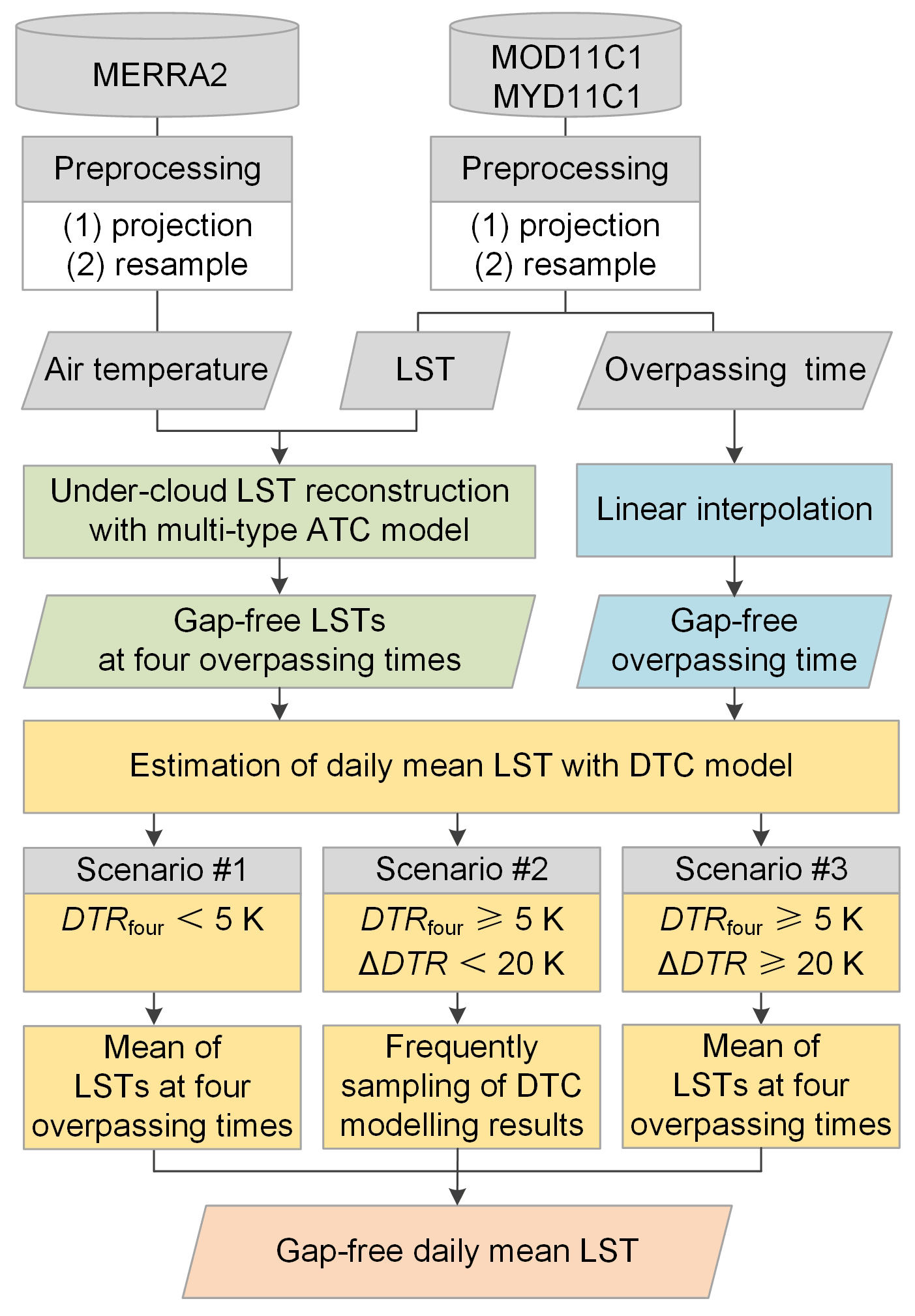
Figure 2 Flowchart of the IADTC framework. DTR_four refers to diurnal temperature range (DTR) calculated as the maximum minus the minimum from the gap-free LSTs at the four overpass times; DTR_DTC refers to the DTR calculated from the hourly LSTs modeled with the DTC model. ΔDTR refers to the absolute difference between DTR_four and DTR_DTC.

3.1.1 Data preprocessing

We generated the global T_dm product with a spatial resolution of 0.5×0.5^∘ rather than a higher resolution (e.g., 1 km), mainly because of the following two aspects. First, our study aims at analyzing the spatial pattern of ΔT_sb and the LST trend at the global scale, i.e., to perform a LST climatology analysis for which a spatial resolution of 0.5^∘ is adequate. Second, the T_dm generation is conducted on a daily and pixel-by-pixel basis on the global scale, which requires a huge amount of computational resources on a higher spatial resolution. Consequently, the MOD11C1 and MYD11C1 products were resampled to a spatial resolution of 0.5^∘; the MERRA2 reanalysis hourly air temperature data were resampled to daily values with the same resolution.

3.1.2 Under-cloud LST reconstruction with multi-type ATC model

The general formula of ATC model is displayed in Eq. (2). The single-type ATC model in the OADTC framework uses a single sinusoidal function (M=1 in Eq. 2) to model the intra-annual LST variations driven by solar radiation change and incorporates surface air temperatures to help simulate the LST fluctuations induced by synoptic conditions (Zou et al., 2018; Z. Liu et al., 2019). The use of a single sinusoidal function is generally acceptable for midlatitude regions. However, a single sinusoidal is no longer suitable for low latitudes because there are two solar radiation peaks within a yearly cycle of low-latitude regions (Xing et al., 2020; Bechtel, 2015; Cao and Sanchez-Azofeifa, 2017); it is also inadequate for high-latitude regions where polar days and nights occur (Østby et al., 2014; Z. Liu et al., 2019; Westermann et al., 2012). Therefore, the use of the single-type ATC model in the OADTC framework is less suitable to generate T_dm at the global scale (Fig. 3). To overcome this limitation, the IADTC framework uses different versions of ATC model (termed the multi-type ATC model) to reconstruct under-cloud LSTs over the low-latitude, midlatitude, and high-latitude regions, respectively. The details are given as follows:

1. Low-latitude regions (23.5^∘ N–23.5^∘ S).

   The solar radiation possesses two peaks within a yearly cycle over low-latitude regions (Fig. 3a). We therefore employed the ATC model with two sinusoidal functions (M=2 in Eq. 2) to reconstruct the daily LST dynamics within an annual cycle (Z. Liu et al., 2019; Xing et al., 2020).

2. Midlatitude regions (23.5^∘–66.5^∘ N/S).

   The solar radiation peaks once in summer during an annual cycle. We therefore employed the ATC model with a single sinusoidal function (M=1 in Eq. 2) to reconstruct the daily LST dynamics (Fig. 3b).

3. High-latitude regions (66.5^∘–90^∘ N/S).

   The polar day/night phenomena occur over high-latitude regions, and the duration increases with latitude. Theoretically, over these regions, the ATC model with multiple sinusoidal functions should be the best choice. However, the number of cloud-free MODIS observations is limited, and additional model complexity can lead to over-fitting and weaken the generalization ability of the ATC model (Z. Liu et al., 2019). To balance model accuracy and generalization ability, the ATC model with two sinusoidal functions was selected for high-latitude regions (see Fig. 3c).

   $$\begin{array}{}\text{(2)}& \left\{\begin{array}{l}{T}_{\mathrm{ATCM}}\left(d\right)=T_{\mathrm{0}}+{\sum }_{m=\mathrm{1}}^M{A}_{\mathrm{m}}\sin \left(\frac{\mathrm{2}\mathit{\pi }md}{N}+{\mathit{\theta }}_{\mathrm{m}}\right)+k\cdot \mathrm{\Delta }{T}_{\mathrm{air}}\left(d\right)\\ \mathrm{\Delta }{T}_{\mathrm{air}}\left(d\right)=T_{\mathrm{air}}\left(d\right)-T_{\mathrm{ATCO}}\left(d\right)\\ T_{\mathrm{ATCO}}\left(d\right)=T_{\mathrm{0}}{}^{\prime }+{\sum }_{m=\mathrm{1}}^M{A}_{\mathrm{m}}{}^{\prime }\sin \left(\frac{\mathrm{2}\mathit{\pi }md}{N}+{\mathit{\theta }}_{\mathrm{m}}{}^{\prime }\right),\end{array}\right.\end{array}$$

   where T_ATCM (d) denotes the daily LST variations simulated with the ATC model; M is the number of harmonic components used; d and N are the day of year (DOY) and number of days in a year, respectively; ΔT_air (d) is the difference between the daily SATs (i.e., T_air (d), obtained from MERRA2 reanalysis data) and the modeled air temperatures with the original ATC model (T_ATCO (d)); and T₀, A_m, θ_m, and k are the parameters that need to be solved with the cloud-free daily LSTs and SATs, usually through the least-squares method.

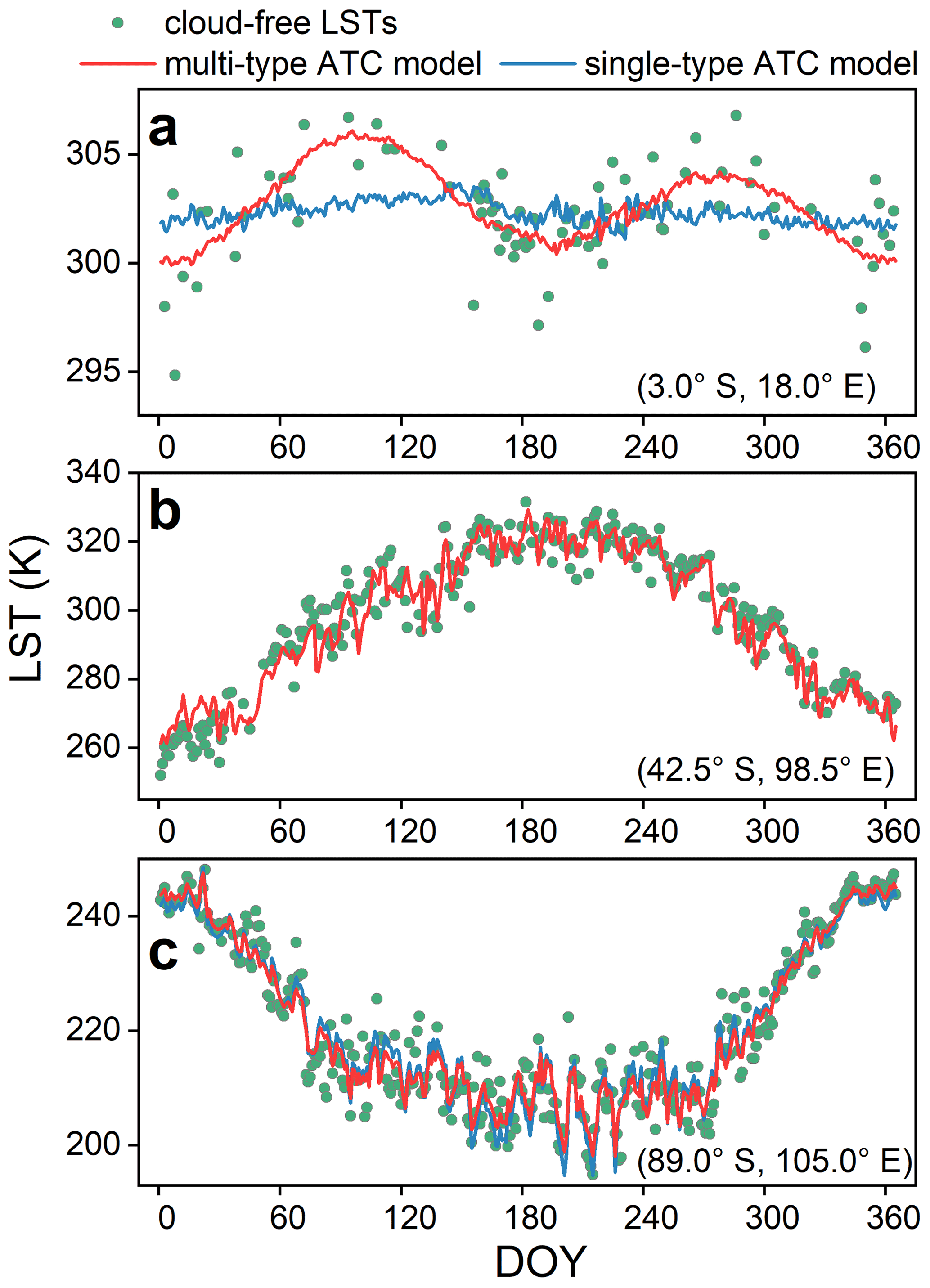
Figure 3 Comparison of reconstructing under-cloud LSTs with multi-type and single-type ATC models at different latitudes. Panels (a, b, c) show three examples of ATC modeling at low-latitudes, midlatitudes, and high-latitudes for cloud-free Terra-day LST in 2019. The green circles, blue lines, and red lines denote the cloud-free observations and LSTs simulated by the single- and multi-type ATC models, respectively. Note that for (b), the results of the single- and multi-type ATC models are identical since they both use the ATC model with a single sinusoidal function.

3.1.3 Interpolation of overpass times

The under-cloud LST reconstruction with the ATC model ensures that there are four valid LSTs within a diurnal cycle. However, there are still missing values for the corresponding four overpass times. We used linear interpolation to reconstruct the missing overpass times based on the valid overpass times on the 2 adjacent days with valid values. For example, if the overpass times from 10 to 20 July for Aqua day are missing, the linear interpolation was used to fill the missing values during this period using the valid values on the 2 adjacent days with valid values (i.e., 9 and 21 July). The uncertainties of linear interpolation are expected to be within the range associated with local overpass time fluctuations. For the low-latitude and midlatitude regions where the overpass time fluctuations are relatively small (less than 1.5 h), the uncertainties using linear interpolation are relatively minor. However, for the high-latitude regions where the overpass times fluctuate significantly (Fig. A1), linear interpolation holds a larger error and might affect the estimation of T_dm. More discussions in terms of the uncertainties of the linear interpolation are provided in Sect. 5.2.

3.1.4 Estimation of daily mean LST with DTC model

The under-cloud LST reconstruction (Sect. 3.1.2) and linear interpolation of overpass time (Sect. 3.1.3) ensure that there are four valid LSTs and the associated overpass times per day. These provide the foundation for estimating T_dm with a four-parameter DTC model. This study selected the four-parameter GOT09-dT-τ model, which has been shown to have the highest accuracy among a variety of four-parameter DTC models (Hong et al., 2018). Further details related to the formulae and the associated parameters of the GOT09-dT-τ model are provided in Göttsche and Olesen (2009) and Hong et al. (2018).

For the generation of global products, the GOT09-dT-τ model can face the issues of no solution or extreme solution, under which the estimated T_dm can be significantly biased due to the reduced capability to model LST around sunrise (Hu et al., 2020) (Fig. 4c). The failed simulations can be associated with the following two reasons: (1) there are four daily MODIS LSTs per daily cycle but no observation around sunrise (Hong et al., 2018); (2) the DTC model is subject to the clear-sky hypothesis (Göttsche and Olesen, 2009). Therefore, to avoid outliers caused by failed simulations, under certain conditions, T_dm was estimated directly by averaging the four LSTs per daily cycle. We introduced two criteria to determine whether to use the DTC model for estimating T_dm or not (Fig. 2, Scenario no. 1 to no. 3).

The first criterion is based on the diurnal temperature range (DTR), which was calculated as the maximum minus the minimum LSTs within a diurnal cycle. Specifically, the DTR calculated by four LSTs within the diurnal cycle (termed DTR_four) was used (Fig. 2). Here these four daily LSTs can consist of both cloud-free observations (T_{in_cloud_free}, the green circles in Fig. 4) and under-cloud LSTs reconstructed by the ATC model (T_{in_ATC}, the blue triangles in Fig. 4). For relatively small DTR_four, e.g., on overcast days with heavy clouds or on days with low incoming solar radiation (e.g., polar nights), T_dm can be directly estimated as the mean of the four daily LSTs per daily cycle (Fig. 4a). In this case, the DTC model would be unnecessary. We empirically set the DTR_four threshold as 5.0 K (see Sect. 5.1 for detailed discussions). In other words, when the DTR_four is less than 5.0 K (see Scenario no. 1 in Figs. 2 and 4a), T_dm estimated with the IADTC framework (termed T_{dm_IADTC}) was obtained by averaging the four LSTs within a diurnal cycle (termed T_{dm_ATC_four}).

When DTR_four is greater than 5.0 K, the DTC model would be used to simulate the diurnal LST dynamics. However, for the global generation of T_dm, the simulation can still fail for cases with complicated diurnal LST dynamics (Fig. 4c). To avoid this issue, we introduced the second criterion to determine whether to use the DTC model or not. This was done by comparing the DTR_four and the DTR calculated by the DTC model (termed DTR_DTC). This comparison can be used to identify the failed simulations of the DTC model because the DTR_DTC would be abnormal once the LSTs modeled by the DTC model are significantly underestimated around sunrise. Therefore, we employed the absolute difference between DTR_DTC and DTR_four (termed as ΔDTR) as the second threshold to further determine whether to use the DTC model or not. This study empirically set the ΔDTR threshold as 20.0 K. More discussions on this are provided in Sect. 5.1.

In the practical generation of T_dm, when DTR_four≥5.0 K and ΔDTR <20.0 K (Scenario no. 2 in Fig. 2), the DTC modeling results (T_{in_ATC_DTC}; see the blue line in Fig. 4b) are satisfactory and were then used to estimate T_dm. The T_{dm_IADTC} was then calculated as the average of instantaneous hourly LSTs (T_{in_ATC_DTC}). When DTR_four≥5.0 K and ΔDTR ≥20.0 K (Scenario no. 3 in Fig. 2), the DTC model may fail (Fig. 4c) as the T_dm estimate based on the DTC modeling (i.e., T_{dm_ATC_DTC}) is considerably lower than the true T_dm. In this case, the error of T_{dm_ATC_DTC} can be even larger than that of T_dm estimated as the average of the four LSTs within the day (i.e., T_{dm_ATC_four}; refer to Fig. 11 in Sect. 5.1). Therefore, in this case, T_{dm_IADTC} was directly calculated as T_{dm_ATC_four}. In summary, for Scenarios no. 1 and 3, T_{dm_IADTC} was calculated as T_{dm_ATC_four}, while it was calculated as T_{dm_ATC_DTC} for Scenario no. 2.

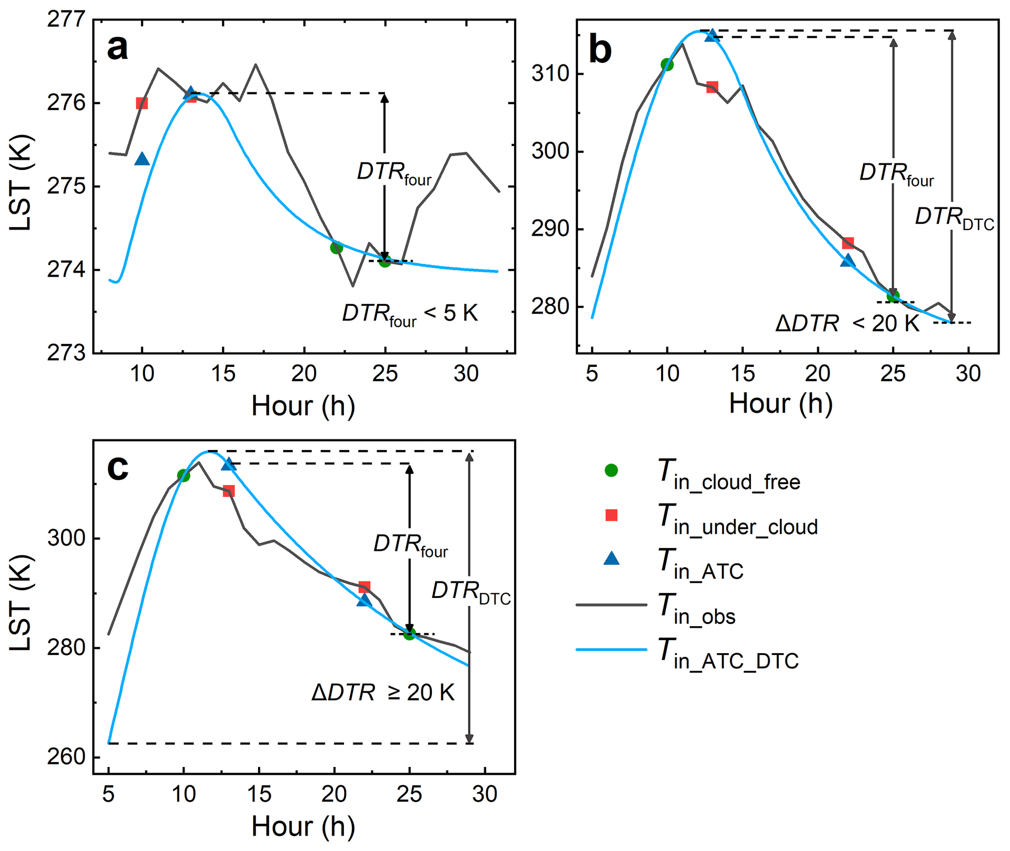
Figure 4 Estimation of T_dm under different conditions. Panel (a) displays an example of estimating T_dm by averaging T_{in_cloud_free} and T_{in_ATC} when DTR_four is less than 5.0 K (i.e., Scenario no. 1); panel (b) displays an example of estimating T_dm based on the DTC modeling results (i.e., Scenario no. 2); panel (c) displays an example of estimating T_dm by averaging T_{in_cloud_free} and T_{in_ATC} when ΔDTR is equal or greater than 20.0 K (i.e., Scenario no. 3). The green circles, red rectangles, and blue triangles denote the instantaneous cloud-free LST observations, under-cloud LST observations, and under-cloud LSTs reconstructed by the ATC model, respectively. The black lines denote the in situ LST observations, while the blue lines show the DTC-modeled values based on the cloud-free LST observations and ATC-modeled under-cloud LSTs. Note that hours larger than 24 along the x axis correspond to the next day.

3.2 Validations

The GADTC products were validated from the following two aspects: (1) validating the IADTC framework indirectly with single-source in situ measurements at the site level and (2) validating the GADTC products directly by comparing with in situ measurements. These two aspects complement each other and allow us to assess the applicability of the IADTC framework and the accuracy of the generated GADTC products. The direct comparison of the GADTC product with in situ measurements (SURFRAD and FLUXNET measurements for this study) provides information on the accuracy of the IADTC framework, especially over homogeneous areas (Guillevic et al., 2018). However, such direct validations can be affected by uncertainties beyond the IADTC framework, e.g., a mismatch of spatial scale between satellite and in situ measurements, different observation angles, and uncertainties from the LST retrieval algorithm (Ermida et al., 2014; Guillevic et al., 2014; Li et al., 2014). Therefore, direct comparisons may not fully reflect the true accuracy of the IADTC framework. To address this issue and assess the applicability of IADTC framework, we validated the IADTC framework indirectly by driving it with in situ measurement and then using hourly measurements for validation. This strategy avoids the mismatch issue of multi-source data and can, therefore, better reflect the accuracy of the IADTC framework (Hong et al., 2021).

3.2.1 Validation of the IADTC framework with in situ measurements

The IADTC framework was validated with in situ hourly measurements obtained exclusively from SURFRAD and FLUXNET data. During this validation process, the MERRA2 air temperature at the corresponding station location, instead of the air temperature from in situ measurements, was used to drive the ATC model, which is identical to the actual generation of the GADTC products.

The approach used the cloud-free in situ measurements at each MODIS overpass time and MERRA2 air temperatures to drive the ATC model and the corresponding under-cloud in situ measurements (T_{in_under_cloud}, red rectangles in Fig. 4) to evaluate the accuracy of the under-cloud LSTs reconstructed by the ATC model (T_{in_ATC}). The accuracy of the T_dm estimated with the IADTC framework (T_{dm_IADTC}) was evaluated against “true” T_dm (termed T_{dm_true}), i.e., the average of the hourly in situ measurements (T_{in_obs}, gray line in Fig. 4). We also provided the sampling bias (ΔT_sb) of the traditional method based on cloud-free observations (i.e., the average of T_{in_cloud_free}), which here is termed T_{dm_cloud_free}. Therefore, the accuracy improvements of T_{dm_IADTC} compared to T_{dm_cloud_free} are reflected in the corresponding reduction of ΔT_sb. We further provide T_dm estimated with the OADTC framework (termed T_{dm_OADTC}) to illustrate the improvement achieved by the IADTC framework.

3.2.2 Validation of the GADTC product directly with in situ measurements

After matching the geolocation and observation time, we directly compared the GADTC product with in situ T_dm measurements from SURFRAD and FLUXNET. Note that outliers in the in situ measurements were removed before performing the accuracy evaluation; here outliers are defined as the T_dm differences between in situ measurements and GADTC products deviating by more than 3σ (3 standard deviations) from the mean (Göttsche et al., 2016; Zhang et al., 2020).

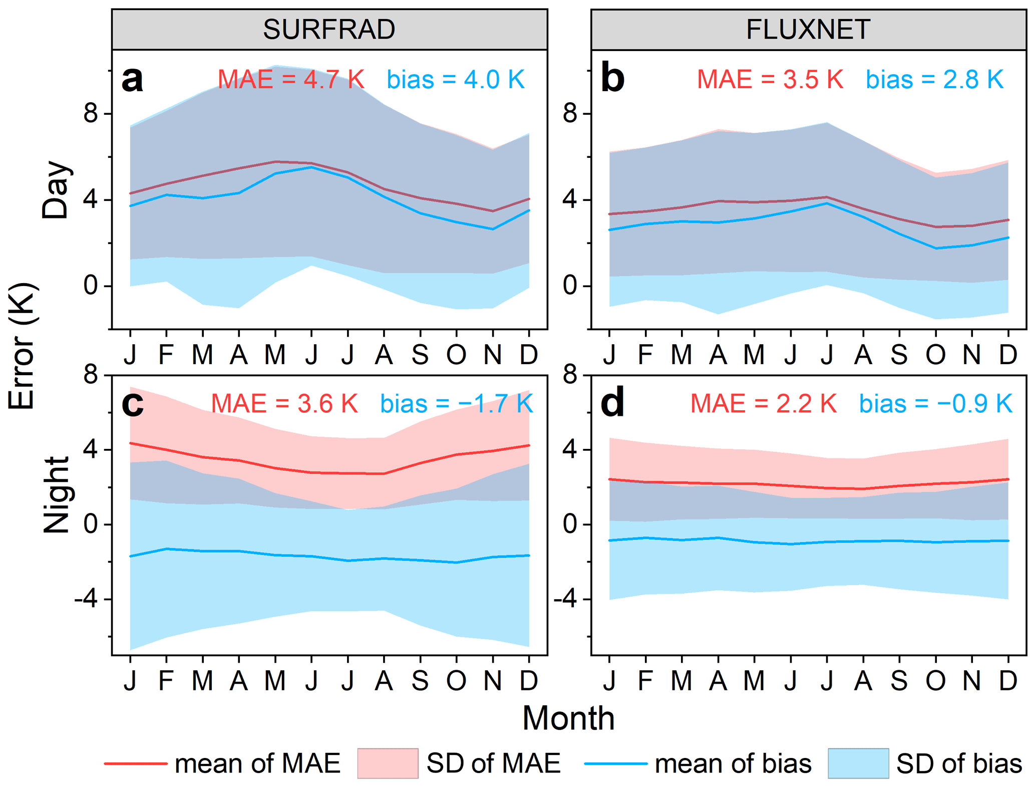
Figure 5 Validations of reconstructed under-cloud LSTs at Aqua and Terra day and night overpass times based exclusively on in situ data. The under-cloud LSTs were reconstructed with the ATC model. Panels (a) and (b) show monthly mean errors obtained for daytime overpasses (including Aqua day and Terra day) for SURFRAD and FLUXNET data, respectively; (c) and (d) show the same for the nighttime overpasses (including Aqua night and Terra night).

3.3 Analysis of the GADTC product

We analyzed the difference in LST values and trends between T_{dm_cloud_free} (the daily mean LST estimated by the traditional method) and the GADTC products. For the difference in LST values, we present the global spatial distribution of ΔT_sb using the GADTC product as the reference (see Sect. 4.3). For the difference in LST trends, the seasonal Mann–Kendall test and Theil–Sen slope were used to diagnose the warming/cooling trend of LST and describe its slope, respectively (see Sect. 4.4). The seasonal Mann–Kendall test is a nonparametric test suitable to detect LST warming/cooling trends and to quantify the associated significance level in LST time series (Hirsch et al., 1982; Hussain and Mahmud, 2019), while the Theil–Sen slope reduces the impact of outliers on LST trend analysis (Sen, 1968; Theil, 1950). We conducted a seasonal Mann–Kendall test for both the T_{dm_cloud_free} and the GADTC product and compared their Theil–Sen slopes in describing global LST trends.

4 Results

4.1 Validation of the IADTC framework with in situ measurements

The validations using the SURFRAD measurements show that the MAE and bias of the ATC model for the day are 4.7 and 4.0 K, respectively, while those for the night are 3.6 and −1.6 K, respectively (Fig. 5a and c). Although the results for the ATC model are less satisfactory, the T_dm accuracies estimated with the IADTC framework are generally acceptable: the MAEs of T_{dm_IADTC} at the daily and monthly scales are 1.4 and 0.6 K, respectively and the corresponding biases are both −0.2 K (Fig. 6). By contrast, the MAEs of the T_{dm_cloud_free} are 4.1 and 2.5 K at the daily and monthly scales, respectively; i.e., they indicate a significantly lower accuracy compared to that of T_{dm_IADTC}.

The proportions of the three scenarios were 0.2 %, 95.0 %, and 4.8 %, respectively. In Scenarios no. 1 and no. 3 under which the accuracies were improved compared with the OADTC framework, the IADTC framework improves the MAE of estimated T_dm by around 0.45 K (from 2.80 to 2.35 K; see Fig. B1a). The accuracy improvement results mainly from two aspects: (1) the IADTC framework reduces the systematic negative bias caused by cases for which the DTC-modeled LSTs are significantly underestimated around sunrise; and (2) the outliers due to failed DTC simulations are avoided. The overall accuracies for all three scenarios show that the IADTC framework improves the bias from −0.38 to −0.18 K, while the MAE improvement is relatively small. The relatively slight increase in the overall accuracy is attributed to the relatively small proportion of Scenarios no. 1 and no. 3 (around 5 %).

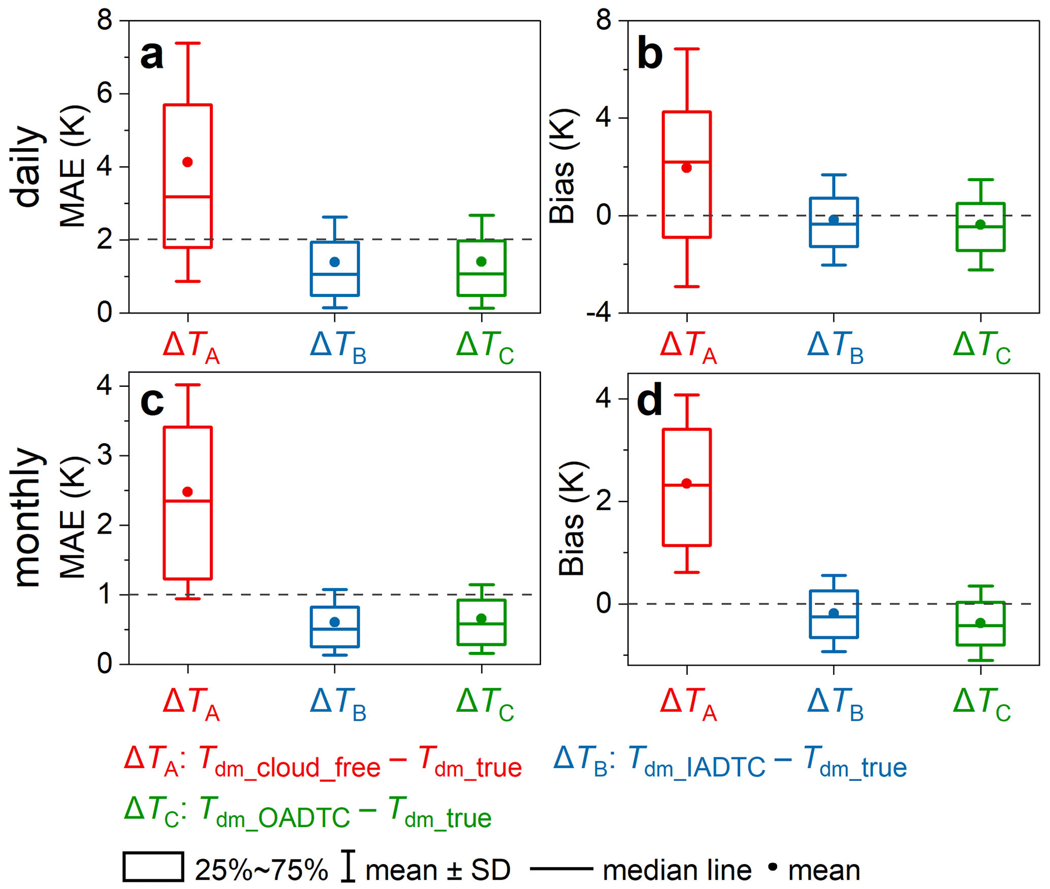
Figure 6 Validations of daily mean LST (T_dm) estimation with SURFRAD data. Box plots show the errors for the traditional T_dm estimation method (T_{dm_cloud_free}), the IADTC framework (T_{dm_ATC_DTC}), and the OADTC framework (T_{dm_OADTC}). Panels (a) and (b) display the MAE and bias at the daily scale, respectively, and panels (c) and (d) display the MAE and bias at the monthly scale, respectively.

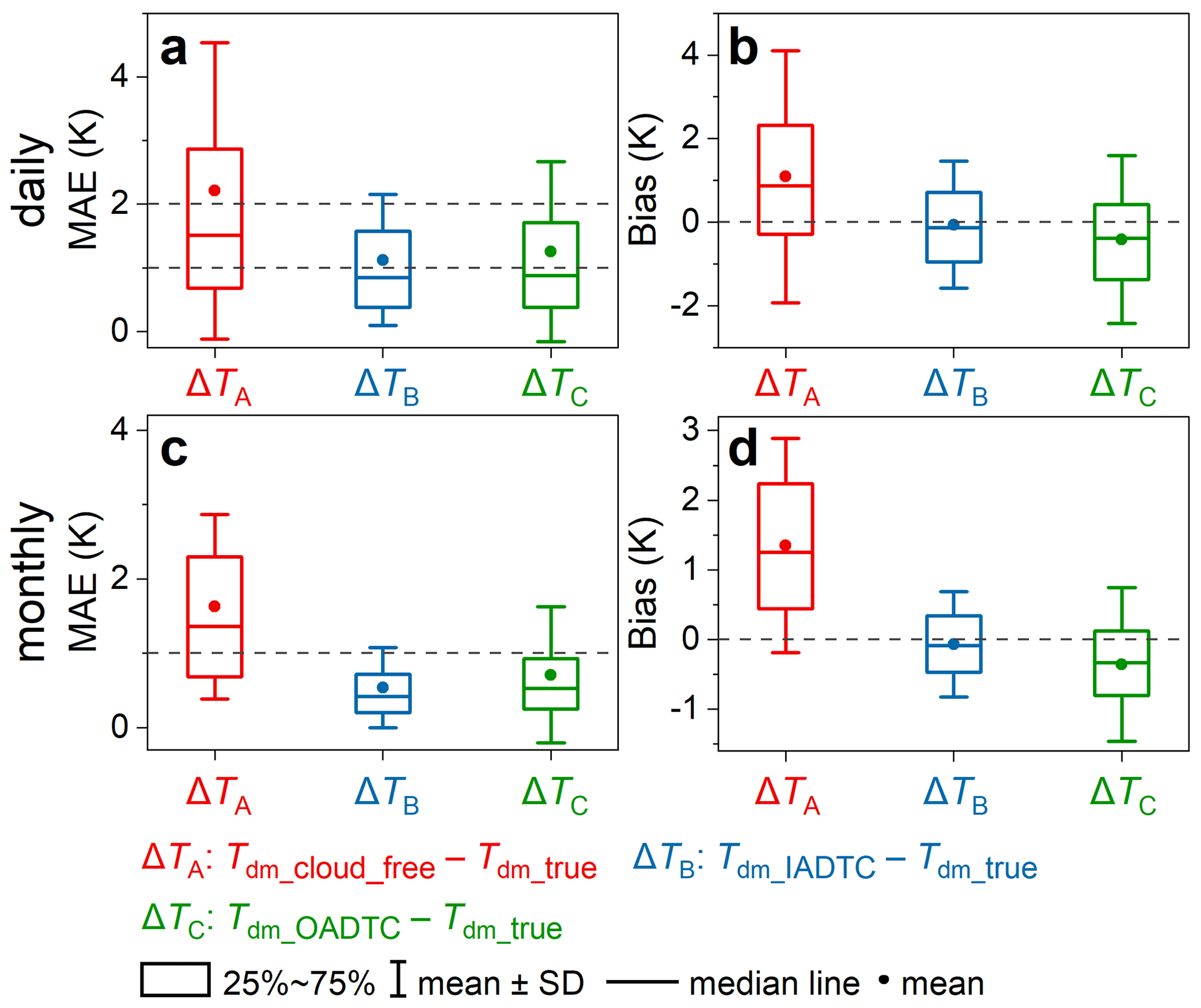
The validations using the FLUXNET data are similar to those with the SURFRAD data: (1) the IADTC framework significantly reduces the ΔT_sb of T_{dm_cloud_free}; (2) the MAEs of T_{dm_IADTC} are 1.1 and 0.5 K at the daily and monthly scales, respectively; and (3) the biases are both close to zero (Fig. 7). The validations again indicate that the under-cloud LSTs reconstructed by the ATC model are systematically positive during the day (the MAE and bias are 3.5 and 2.8 K, respectively) and systematically negative during the night (the MAE and bias are 2.2 and −0.9 K, respectively) (Fig. 5b and d).

The proportion of each scenario is 10.2 %, 82.5 %, and 7.3 %, respectively. Compared with the OADTC framework, in Scenarios no. 1 and no. 3 (the proportion is 17.4 %) under which the accuracies are considerably improved, the IADTC framework improved the MAE of the estimated T_dm by around 0.78 K (from 1.95 to 1.17 K; refer to Fig. B1b). However, for all the three scenarios, the overall MAE and bias improvements of the IADTC framework are around 0.15 and 0.30 K, respectively (Fig. 7).

Figure 7 The same as Fig. 6 but for the FLUXNET data.

4.2 Evaluation of the GADTC product with in situ measurements

The comparison between the GADTC products and in situ measurements (SURFRAD and FLUXNET datasets) shows that the MAEs of the GADTC products are 3.0 and 2.6 K at the daily and monthly scales, respectively, and the mean bias on both scales is −1.5 K (Fig. 8). The MAE and bias are larger than those of the IADTC framework at site level (Fig. 6). This is thought to be due to inconsistencies between MODIS cloud-free observations and in situ measurements, i.e., errors of MODIS cloud-free observations propagating into the GADTC products. The mismatch in spatial resolution between the GADTC products and in situ measurements can also lead to lower accuracies.

The validation with the SURFRAD measurements show that the MAE of the GADTC products is 2.2 and 1.6 K at the daily and monthly scales, respectively, and the bias is around −1.6 K at both scales (Fig. 8a and d). These accuracies of daily mean LST are generally on a par with those of instantaneous LSTs in studies comparing instantaneous MODIS cloud-free observations and SURFRAD measurements (Duan et al., 2019; Martin et al., 2019). Across the different SURFRAD sites, the MAEs of the GADTC products are relatively similar (around 2.2 K; see Table 1).

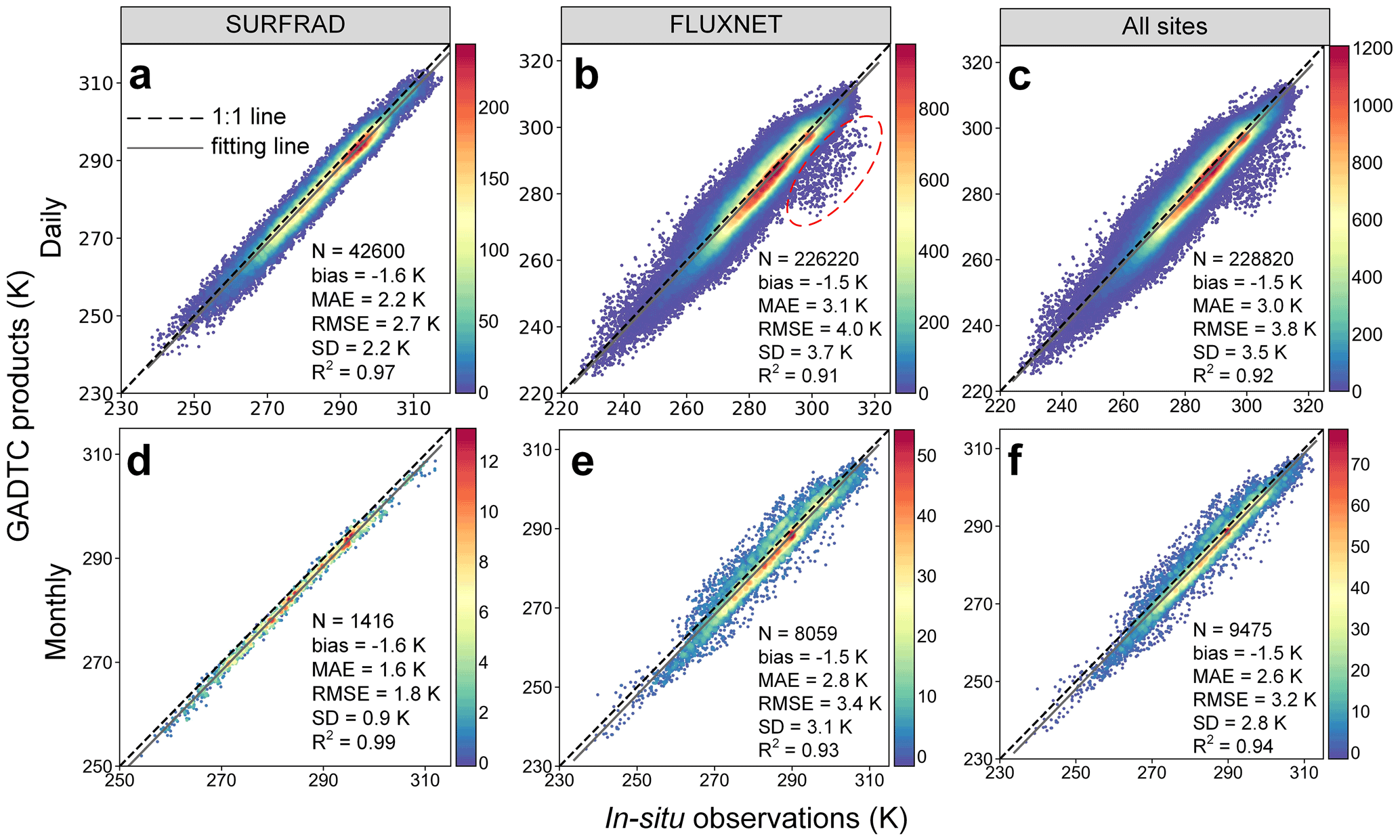
Figure 8 GADTC products versus in situ observations. Panels (a), (b), and (c) compare the daily mean LST over the SURFRAD, FLUXNET and combined sites, respectively, and panels (d), (e), and (f) show the corresponding results for monthly mean LST. The biases were calculated by the GADTC products minus the in situ measurements. The red ellipse in (b) highlights the cases with notably large errors.

Table 1 Validation results obtained over the seven SURFRAD sites.

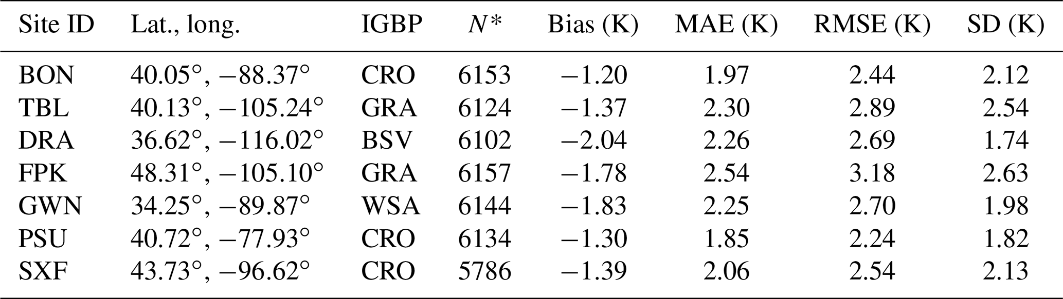
^* N denotes the number of days used for validation.

The direct comparison between the GADTC products and FLUXNET measurements shows that the MAEs are 3.1 and 2.8 K at the daily and monthly scales, respectively, and the bias at these two timescales is −1.5 K (Fig. 8b and e). Compared with the validations over the SURFRAD sites, the accuracies over the FLUXNET sites decrease slightly, and the standard deviations increase. The relatively larger errors at several FLUXNET sites (e.g., AU-Wac, SJ-Adv, and CH-Fru sites, with MAEs larger than 8.0 K; refer to the red ellipse in Fig. 8e) partly account for the lower accuracy. The relatively large errors at these sites might be related to the erroneous in situ measurements as well as the high spatial heterogeneity around these sites. However, the accuracies at most FLUXNET sites are acceptable.

The validations over the FLUXNET sites show that the MAEs vary from 2.6 to 4.8 K and depend on land cover type. Relatively lower accuracies of the GADTC products (MAE larger than 3.5 K) are observed over IGBP land cover types OSH (open shrublands) and SNO (snow and ice) (Table 2). This may be related to unusually large measurement errors and the relatively high spatial heterogeneity at some sites as well as the limited number of sites representing a particular land cover type. For example, the accuracy assessment over the SNO land cover type is performed with a single site, and there are only three sites of the OSH land cover type (e.g., the RU-Cok with MAE as large as 4.6 K).

Table 2 Validation results for the GADTC products stratified by IGBP land cover type of the FLUXNET sites.

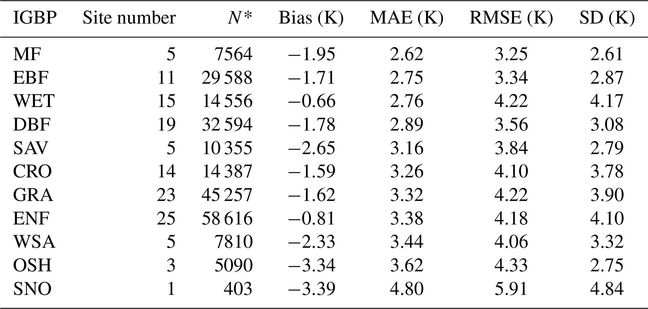
^* N denotes the number of days used for validation.

4.3 Analysis of the GADTC product

The validations based exclusively on in situ LST measurements (Fig. 6) show that the IADTC framework can reduce the sampling bias (ΔT_sb, i.e., T_{dm_cloud_free}−T_{dm_true}) significantly, especially at the monthly scale. ΔT_sb directly affects the value of T_dm and may further influence the LST trend. Therefore, based on the GADTC products, we analyzed the global distribution of ΔT_sb (calculated by T_{dm_cloud_free}−T_{dm_IADTC}) at the monthly scale (Sect. 4.3.1) and compared the LST trend differences between monthly averaged T_{dm_cloud_free} and T_{dm_IADTC} to study the impact of ΔT_sb on LST trends (Sect. 4.3.2).

4.3.1 Global distribution of the sampling bias ΔT_sb

The global distribution of the averaged ΔT_sb from 2003 to 2019 shows that the global-mean ΔT_sb is 1.8 K (Fig. 9). At low-latitude and midlatitude regions, ΔT_sb is generally around 2.0 K, yet it can exceed 4.0 K in some regions, e.g., deserts. At high-latitude regions, ΔT_sb is close to or slightly less than zero. ΔT_sb also varies with month or season (Fig. C1). For example, the average ΔT_sb for September–October–November (2.0 K) is larger than that for December–January–February (1.5 K). We further observe that ΔT_sb is sensitive to land cover type and that DTR can partially explain ΔT_sb. For instance, regions with a large DTR (e.g., deserts or bare soils) usually have a greater ΔT_sb (Sharifnezhadazizi et al., 2019; Hong et al., 2021; Jin and Dickinson, 2010).

Apart from the DTR, in high-latitude regions, ΔT_sb can also be affected by the drift of MODIS overpass time. The DTR is relatively small in high-latitude regions where the angle of the incident solar radiation is low and the LST observations across a diurnal cycle are often already close to the true T_dm, leading to a relatively small ΔT_sb. The time drift at high-latitude regions can also contribute to the relatively small ΔT_sb. At low-latitude and midlatitude regions, MODIS samples the surface near 10:30, 13:30, 22:30, and 01:30 (local solar time) (Fig. A1): the systematic positive ΔT_sb is then mostly due to the under-sampling of the nighttime cooling until the sunrise of the next day (Hong et al., 2021). At high-latitude regions, the time drift effect allows MODIS observations to be conducted at other than these four times and alleviates the under-sampling of nighttime cooling, thereby reducing ΔT_sb.

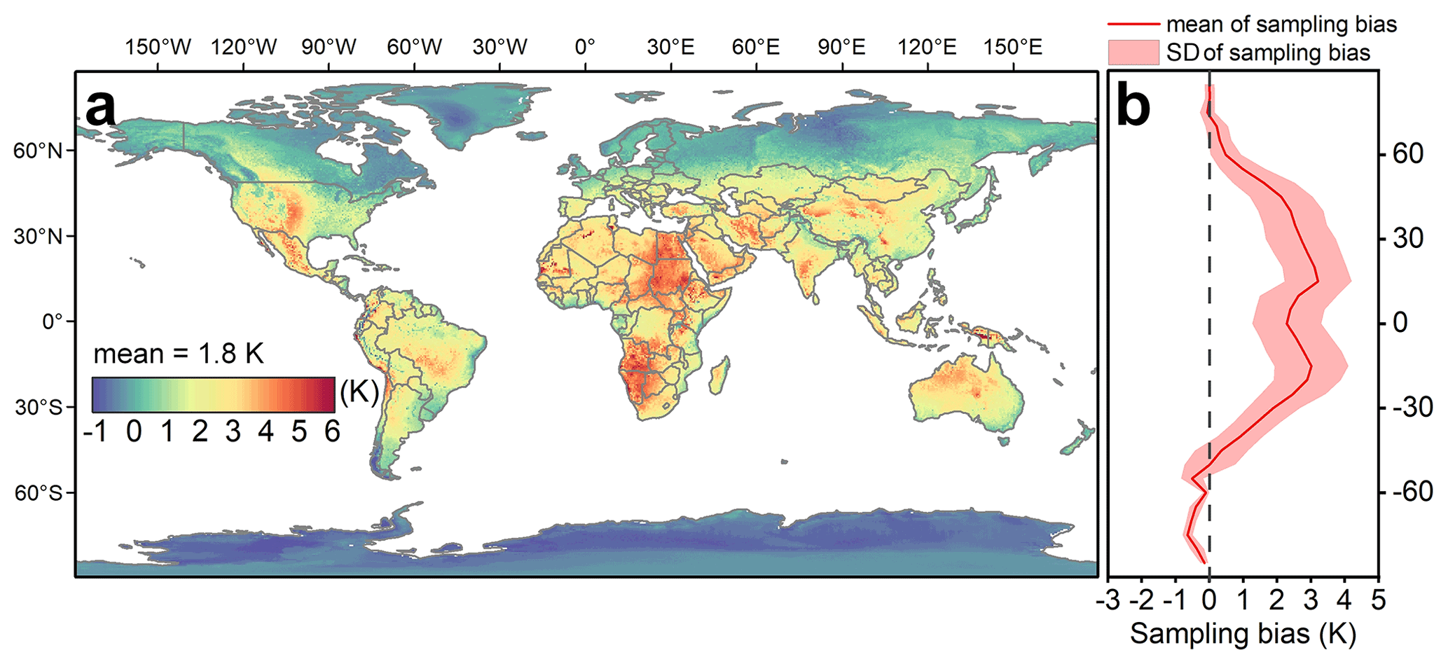
Figure 9 Average sampling bias ΔT_sb from 2003 to 2019. (a) Global spatial distribution of ΔT_sb and (b) average results for 5^∘ longitudinal intervals.

4.3.2 Analysis of global LST trends from 2003 to 2019

The LST trends determined for T_{dm_cloud_free} and T_{dm_IADTC} show similar global patterns; i.e., both can show comparable warming/cooling trends (Fig. 10a and b). For example, they both display an overall increasing LST trend over the globe as well as an accelerated surface warming trend over the Arctic and Europe (Fig. 10), which is consistent with most previous studies (Mao et al., 2017; Sobrino et al., 2020a, b).

However, the slopes of the LST trends are significantly different between T_{dm_cloud_free} and T_{dm_IADTC} with a MAE of 0.012 K yr⁻¹ (Fig. 10e). The slope difference is related to the variation of ΔT_sb, which can be affected by the cloud percentage and cloud duration among different months. When taking the slope of T_{dm_IADTC} as reference, the slope of T_{dm_cloud_free} underestimates the global LST warming rate by 0.004 K yr⁻¹. With the original MODIS LST observations (i.e., T_{dm_cloud_free}) as reference, the warming LST trends would be underestimated over South America, Africa, Asia, and Oceania. They would be overestimated over Europe and relatively similar to the trends obtained with T_{dm_IADTC} over North America and Antarctica.

Figure 10 Global LST trends from 2003 to 2019. Panels (a) and (b) display the global LST trends based on T_{dm_cloud_free} and their averaged results for 5^∘ longitudinal intervals, respectively; panels (c) and (d) show the corresponding results for T_{dm_IADTC}; and panels (e) and (f) show the global LST trend differences between T_{dm_cloud_free} and T_{dm_IADTC} and their averages for 5^∘ longitudinal intervals, respectively.

5 Discussion

5.1 Empirical determination of the threshold for optimizing the T_dm estimation with DTC model

To determine the threshold for the first criterion (i.e., the threshold for the DTR_four; see Fig. 2), we analyzed the variations in the error of T_{dm_ATC_four} depending on DTR_four using SURFRAD and FLUXNET data (Fig. 11). The assessments show that the errors of T_{dm_ATC_four} generally increase with DTR_four. The linear fitting lines show that the error of T_{dm_ATC_four} is relatively low when DTR_four is small. In other words, the direct average of the four LSTs per daily cycle (T_{dm_ATC_four}) is a good estimate of T_dm when the DTR_four is small. Based on the linear fits in Fig. 11a, b, and c, we therefore chose the DTR_four threshold of the first criterion to be 5.0 K.

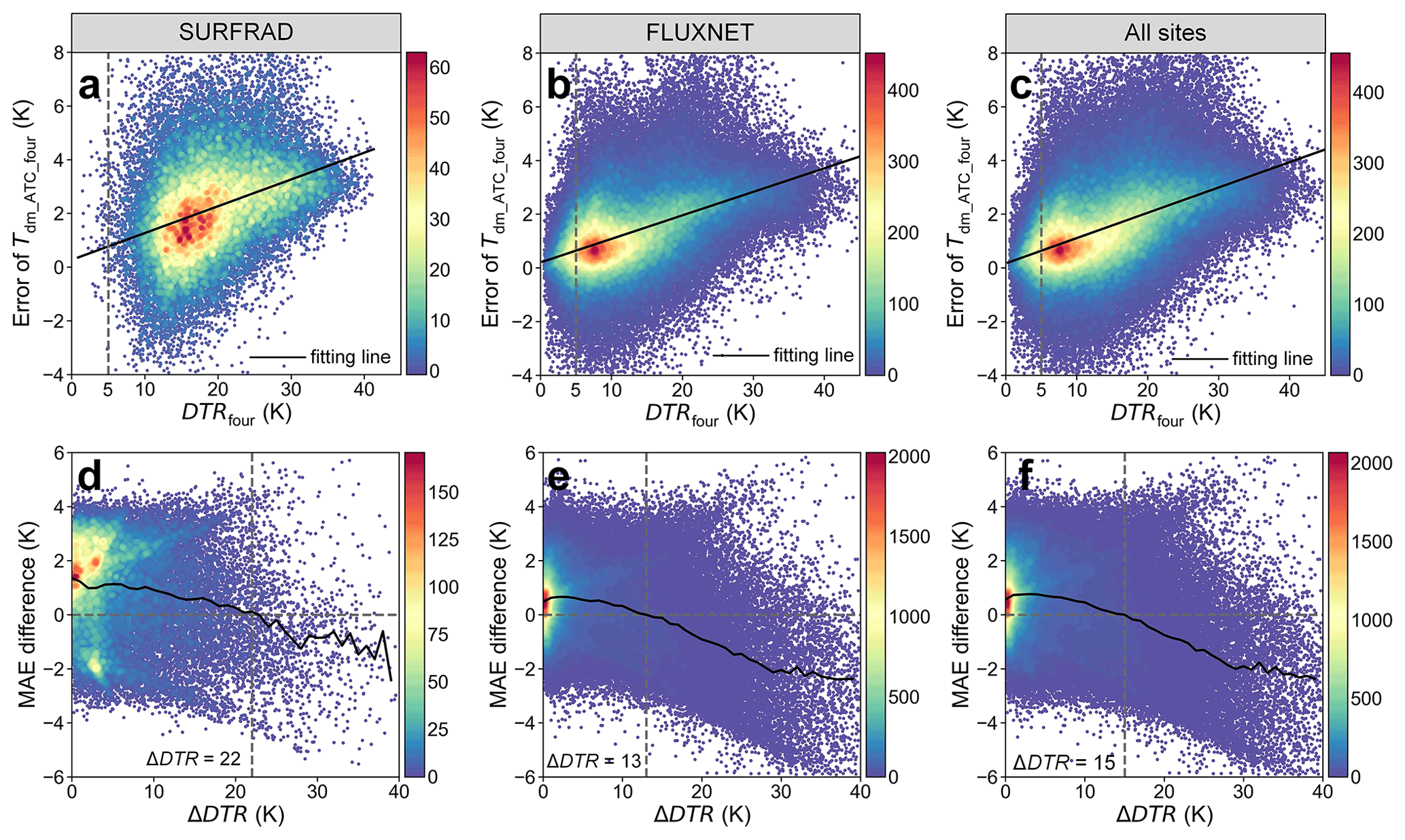
Figure 11 Threshold determination for the two criteria in Fig. 2. Panels (a), (b), and (c) display the errors of T_{dm_ATC_four} (T_{dm_ATC_four} minus T_{dm_true}) depending on DTR_four for SURFRAD, FLUXNET, and combined data, respectively; and panels  (d), (e), and (f) display the MAE differences between T_{dm_ATC_four} and T_{dm_ATC_DTC} (i.e., the MAE of T_{dm_ATC_four} minus the MAE of T_{dm_ATC_DTC}) depending on the ΔDTR for SURFRAD, FLUXNET, and combined data, respectively. The black lines in (d), (e), and (f) denote the averaged MAE difference within every unit along the x axis.

The second criterion uses the ΔDTR to filter cases for which T_dm is significantly underestimated. To determine the optimal threshold for ΔDTR, we analyzed the MAE differences between T_{dm_ATC_four} and T_{dm_ATC_DTC} (i.e., the MAE of T_{dm_ATC_four} minus the MAE of T_{dm_ATC_DTC}) and their dependence on ΔDTR for SURFRAD and FLUXNET data (Fig. 11d and e). The assessments show that ΔDTR is generally less than 10 K, and the accuracy of T_{dm_ATC_DTC} is better than that of T_{dm_ATC_four}. However, with the increase of ΔDTR, the overall accuracy of T_{dm_ATC_four} can be superior to T_{dm_ATC_DTC}. For SURFRAD data, the overall accuracy of T_{dm_ATC_four} is better than that of T_{dm_ATC_DTC} once ΔDTR exceeds 22.0 K (i.e., the ΔDTR threshold is 22.0 K), while this threshold is 13.0 K for FLUXNET data. With the further increase of ΔDTR, the accuracy of T_{dm_ATC_DTC} can be even lower than that of T_{dm_ATC_four}, e.g., by up to 2.0 K in Fig. 11d and e. In other words, T_dm can be estimated more accurately with T_{dm_ATC_four} than T_{dm_ATC_DTC} once ΔDTR is relatively large (i.e., Scenario no. 3).

Note that the optimal threshold of ΔDTR for the SURFRAD data (22.0 K) differs from that for the FLUXNET data (13.0 K). Here, we set the ΔDTR threshold as 20.0 K, which is close to that determined for the SURFRAD data, mostly because of the following factors: (1) the SURFRAD sites have been managed uniformly by NOAA (National Oceanic and Atmospheric Administration) for over 15 years, and the associated radiance measurements have been consistently quality-controlled (Augustine et al., 2000); and (2) the land cover types of the SURFRAD sites are not limited to vegetation. We acknowledge that using a single threshold of 20.0 K may not be optimal for all climate zones and land cover types across the globe, but use of a single threshold effectively avoids outliers due to failed simulations while keeping the simplicity in the global generation of T_dm products.

With the thresholds given as above, we provide the percentage of each scenario within each 10^∘ latitude zone (Fig. 12). In low-latitude and midlatitude regions, the percentage of Scenario no. 2 (i.e., DTR_four≥5.0 & ΔDTR <20.0 K) reaches over 80 %, indicating that the IADTC framework mainly uses the DTC-modeled results to estimate T_dm in those regions. With the increase of latitude, the percentage of Scenario no. 1 (i.e., DTR_four<5.0 K) gradually increases, mostly due to a decrease in DTR with the weakened incoming solar radiation over higher-latitude regions. The percentage of Scenario no. 1 reaches around 60 % in the Arctic and Antarctic, which echoes well with the small ΔT_sb in high-latitude regions (Fig. 9). The percentage of Scenario no. 3 (i.e., DTR_four≥5.0 & ΔDTR ≥20.0 K) remains relatively stable at around 10 % over most regions across the globe, but it can increase to 20 % in the equatorial zone (10^∘ N–10^∘ S) and Antarctic, which indicates the relatively poor performance of the DTC model over these regions. The lower performance of the DTC model in the equatorial zone may be related to the high cloud percentage, while over the Antarctic, it reflects the expected difficulties over polar regions (see Sect. 5.2 for more discussions).

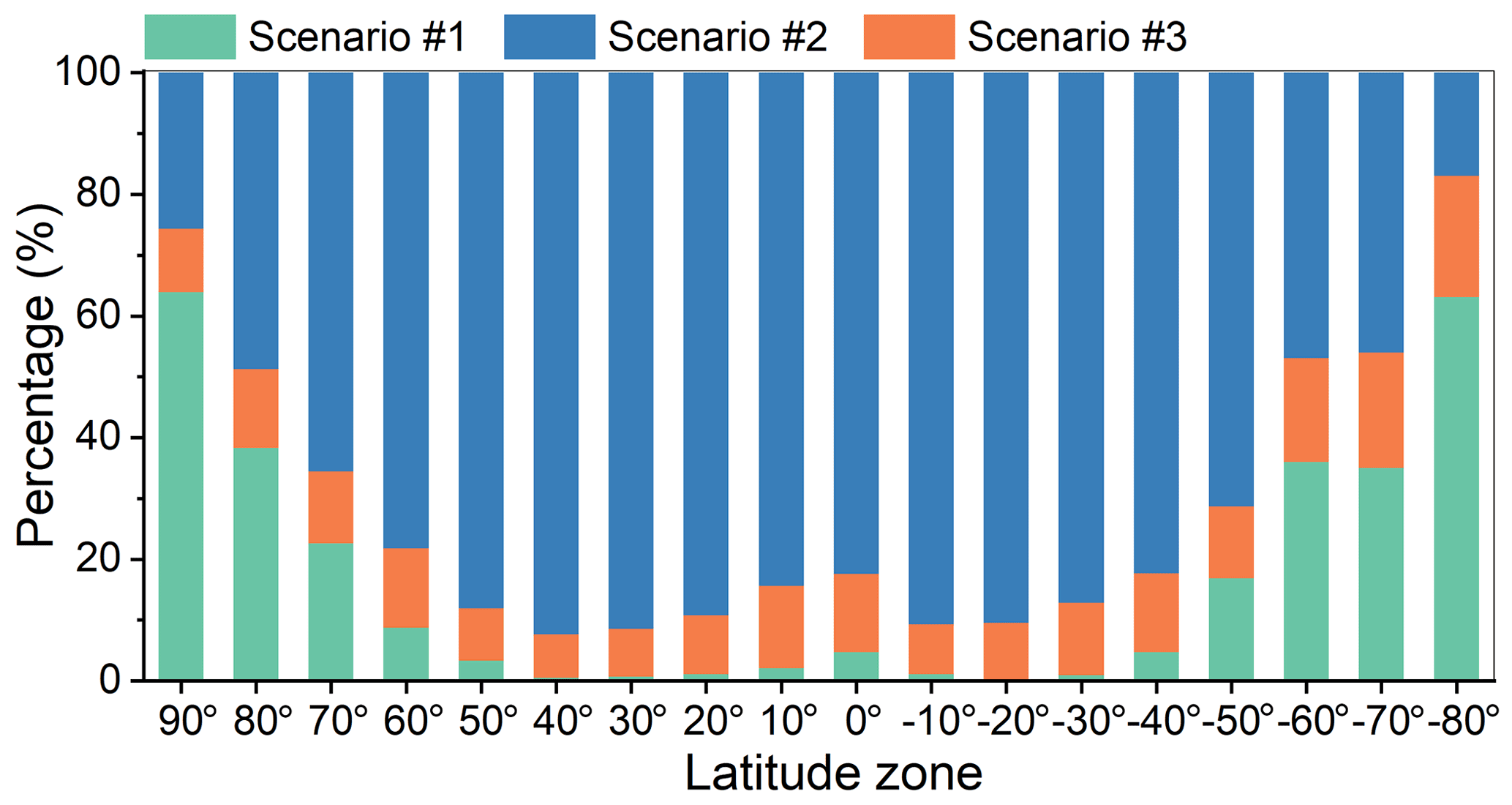
Figure 12 Percentage of each scenario (see Fig. 2) within 10^∘ latitude intervals. For example, the number “−50” denotes the averaged percentage of each scenario within 50 to 60^∘ S.

5.2 Possible uncertainty sources of GADTC product

GADTC products uncertainties arise from four main sources: (1) MODIS data quality or LST retrieval error, (2) cloud cover and contamination; (3) overpass time drift and linear interpolation, and (4) uncertainties associated with the IADTC framework. These four uncertainty sources can affect the under-cloud LST reconstruction with the ATC model as well as the diurnal LST dynamics modeling with the DTC model and, consequently, affect the accuracy of the GADTC products. In addition, these uncertainties can influence each other via error propagation. In the following, we discuss the four error sources and their effect in more detail.

The ATC and DTC models use cloud-free LST observations to estimate T_dm. Therefore, retrieval errors of MODIS LSTs affect the results of ATC and DTC models and the accuracies of the estimated T_dm. Figure A2a shows that the quality of MODIS LSTs in the equatorial regions is lower than that in the other regions. This suggests that GADTC products should have larger uncertainties in equatorial regions where, consequently, the IADTC framework may need further improvements.

Cloud percentage can also impact the accuracies of the GADTC products. In regions with a higher cloud percentage, e.g., the equatorial regions (Fig. A2b), more under-cloud LSTs need to be reconstructed with the ATC model. However, errors of reconstructed under-cloud LSTs are larger than those of cloud-free LSTs. Therefore, regions with a higher cloud percentage are also associated with larger errors from ATC modeling and, consequently, DTC modeling and the estimated T_dm. In polar regions, the cloud detection algorithm has larger uncertainties due to the spectral similarities between clouds and snow (Østby et al., 2014; Westermann et al., 2012), which introduces additional uncertainties to the GADTC products.

The impact of the overpass time drift mainly occurs over high-latitude regions where the time drift is larger. On the one hand, the cloud-free observations used for solving the free parameters of the ATC model come from significantly different times within a daily cycle (Fig. A1), which affects the under-cloud LST reconstruction. On the other hand, approximately 30 % of the T_dm over high-latitude regions were estimated with the DTC modeling results (i.e., Scenario no. 2; refer to Fig. 12), and the time drift can affect the shape of the DTC curve and, therefore, the estimated T_dm. Temporal normalization methods can adjust the LST observations at fluctuated overpass time to the fixed time, which can eliminate the uncertainties in the under-cloud LST reconstruction and diurnal LST dynamics modeling (Ma et al., 2022; Z. Liu et al., 2019; Duan et al., 2014).

The uncertainties of the GADTC products derived with the IADTC framework mainly include three parts: the reconstruction error of the ATC model, the fitting error of the DTC model, and the choice of the two thresholds. First, the currently used ATC model reconstructs under-cloud LSTs during the day (night) with small positive (negative) biases (Fig. 5), even though information on under-cloud air temperature has been incorporated (Z. Liu et al., 2019). Additionally, the errors in the ATC model can affect the determination of scenarios and, consequently, the way to calculate the T_dm. Second, the DTC model assumes clear-sky conditions and is less capable of simulating under-cloud LST dynamics accurately, which introduces additional uncertainties, especially under some complex situations (Hong et al., 2021). Third, the two fixed thresholds for DTR_four and ΔDTR were determined empirically (Fig. 11): the threshold for DTR_four may introduce additional uncertainty over high-latitude regions with small DTRs, while the threshold for ΔDTR may still miss some cases with unrealistic modeling results.

It is difficult to distinguish and quantify the individual contributions of these four uncertainty sources to the estimated T_dm, as they can affect the ATC and DTC modeling individually and interactively. We are therefore unable to provide a quality control flag for each pixel of the GADTC products. The validations have shown that the accuracies of the GADTC products are generally acceptable over most areas across the globe. However, there are relatively larger uncertainties over equatorial and polar regions, where further validations of the GADTC products and an optimization of the IADTC framework are required.

5.3 Future perspectives

Further improvements of the GADTC product can focus on the following three aspects:

1. More extensive validation and inter-comparison of the GADTC products. The GADTC products have been evaluated with FLUXNET and SURFRAD datasets, which include in situ measurements from most climate zones. However, the number of sites is very limited in regions where the uncertainties of the GADTC products are largest (e.g., equatorial and polar regions; refer to Fig. 1). It is therefore hard to validate the IADTC framework as well as its improvements over these regions, e.g., the use of a multi-type ATC model instead of a single-type ATC model. The current in situ data are also insufficient to verify the accuracies of the GADTC products over these regions. It is therefore necessary to obtain more in situ measurements over these regions to validate the accuracy of IADTC framework as well as the GADTC product more completely. Furthermore, reanalysis data, which provide long-term spatiotemporally seamless LSTs and have been widely used in relevant studies (Simmons et al., 2017), can be used to assess the GADTC products (Trigo et al., 2015).

2. Rapid generation of high-resolution spatiotemporally seamless T_dm product. Considering the limited computing resources as well as the aim of this study to obtain the spatial distribution of ΔT_sb and LST trends on a global scale, the spatiotemporally seamless daily T_dm values were generated at a spatial resolution of 0.5^∘. However, the current IADTC framework is equally suitable to generate spatiotemporally seamless daily 1 km T_dm. For local-scale studies, the IADTC framework can probably be applied directly, while for large-scale (continent-scale or even global-scale) studies or applications, the generation of 1 km spatiotemporally seamless daily T_dm could be computationally unaffordable. Under this circumstance, apart from using as many computation resources as possible, we can resort to three strategies to substantially reduce computational complexity.

   First, the similarity of the ATC and DTC model parameters among neighboring pixels can be utilized to accelerate the calculation speed considerably (Hong et al., 2021; Hu et al., 2020; Zhan et al., 2016). Second, the physically based IADTC framework can also be integrated with some statistical or empirical estimation strategies (both on T_dm or on ΔT_sb) to help improve the computational efficiency (Xing et al., 2021). This is reasonable as ΔT_sb (and T_dm) is generally related to local surface properties (Figs. 9 and 11). For example, for large-scale or global high-resolution generation of spatiotemporally seamless daily 1 km T_dm, the IADTC framework can be run in some chosen sample regions to obtain adequate training samples of T_dm (or ΔT_sb). Based on these samples, statistical relationships between T_dm (ΔT_sb) and the related variables such as the four daily LSTs, latitude, land cover type, elevation, and cloud percentage can be obtained to help estimate the T_dm (ΔT_sb) across the globe efficiently. Furthermore, the training samples of T_dm (ΔT_sb) can also be from geostationary satellite data, which can help reduce the computational complexity of the DTC modeling. Third, other highly efficient under-cloud LST reconstruction methods, such as statistical interpolation, spatiotemporal fusion, and the passive microwave-based method (Wu et al., 2021; Hong et al., 2021), or the generated under-cloud LST products (Zhang et al., 2022; Zhao et al., 2020) can replace the ATC model in the T_dm generation framework. Similarly, more efficient diurnal LST dynamics modeling methods can also replace the DTC model (Jia et al., 2022).

3. Generation of T_dm with a longer time span. The GADTC products can only date back to 2003 because the IADTC framework requires four observations per day to estimate T_dm, while MODIS started to provide four daily observations in 2003. However, daily mean LSTs with a longer time span are strongly required for relevant studies such as climate change analysis (Jin and Dickinson, 2010; Simmons et al., 2017). AVHRR data provide global LST observations before 2000, and recent studies have achieved tremendous progress in the correction of orbit drift in order to generate more accurate AVHRR LST datasets (Julien and Sobrino, 2012; Latifovic et al., 2012; Ma et al., 2020; X. Liu et al., 2019). However, the current IADTC framework is not applicable to AVHRR since it only samples the surface twice per day. It is therefore imperative to develop a framework for T_dm estimation that also suits AVHRR-like LSTs. Apart from polar orbiters, geostationary satellites and reanalysis data deliver LST over similar time spans. Although reanalysis data are still limited by their coarse spatial resolution and geostationary satellite data have a limited spatial coverage, especially over polar regions, the fusion of these datasets has great potential to help generate T_dm with a longer time span (Long et al., 2020; Quan et al., 2018).

6 Data availability

The generated GADTC products are organized yearly and are freely available at https://doi.org/10.5281/zenodo.6287052 (Hong et al., 2022). Each file contains the global day-to-day spatiotemporal seamless daily mean land surface temperature in units of kelvin.

7 Conclusions

MODIS LST products have been widely used for long-term time-series analyses. However, due to the missing LSTs caused by clouds and under-sampling of the diurnal LST dynamics, currently there is still no global dataset of spatiotemporally seamless daily mean LST (T_dm) with an acceptable systematic sampling bias (ΔT_sb), which is caused by averaging only instantaneous cloud-free observations. To resolve this issue, we proposed the IADTC framework by using a more advanced ATC model as well as by optimizing the estimation of T_dm with the DTC model and generated global spatiotemporally seamless T_dm products (i.e., the GADTC products) from 2003 to 2019. Based on SURFRAD and FLUXNET in situ measurements, the IADTC framework was validated with in situ measurements at the site level, and the GADTC products were directly compared with in situ T_dm observations. The validations with the SURFRAD and FLUXNET measurements reveal that the IADTC framework is able to reduce the systematic positive sampling bias (ΔT_sb) of T_{dm_cloud_free}, avoid the outliers caused by failed simulation, and provide relatively accurate estimates of spatiotemporally seamless T_dm. Based on the GADTC products, we analyzed the global distribution of ΔT_sb and examined the similarities and differences between the GADTC products and T_{dm_cloud_free} (daily mean LST based on cloud-free observations).

Our major conclusions are as follows: (1) the validations of the IADTC framework based exclusively on in situ measurements at the site level show MAEs of 1.4 and 1.1 K for the SURFRAD and FLUXNET measurements, respectively; the biases for these two datasets are both close to zero. (2) The comparisons between the GADTC satellite products and in situ T_dm observations show that the MAEs for the SURFRAD and FLUXNET measurements are 2.2 and 3.1 K, respectively; the associated biases for these two datasets are −1.6 and −1.5 K, respectively. (3) The global-mean sampling bias ΔT_sb is 1.8 K; it is usually larger than 2.0 K over low-latitude and midlatitude regions and close to zero over high-latitude regions. (4) Global-mean LST trends derived with the GADTC product and the traditional direct-averaging method are similar (both between 0.025 to 0.029 K yr⁻¹ from 2003 to 2019), while the pixel-based MAE in LST trend derived with these two methods is 0.012 K yr⁻¹. Despite its limitations, the proposed IADTC framework allows for the practical generation of global spatiotemporally seamless T_dm and provides insights for generating global long-term high-resolution (e.g., 1 km) T_dm products. The generated GADTC product should be helpful for relevant applications such as climate change analysis and thermal environment investigations.

Appendix A: Statistics on the original MODIS MXDC1 V6 products

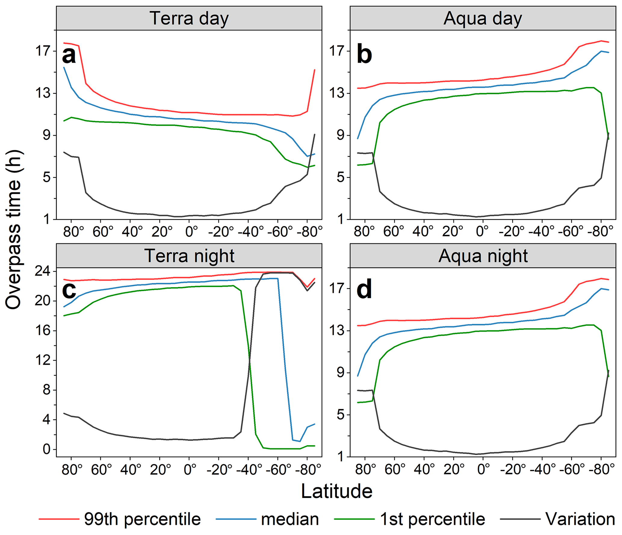
Figure A1 Statistics on each MODIS overpass time within a 10^∘ interval from 2003 to 2019. Each subplot displays the 99th percentile, median, first percentile, and the associated variation (the 99th percentile minus first percentile).

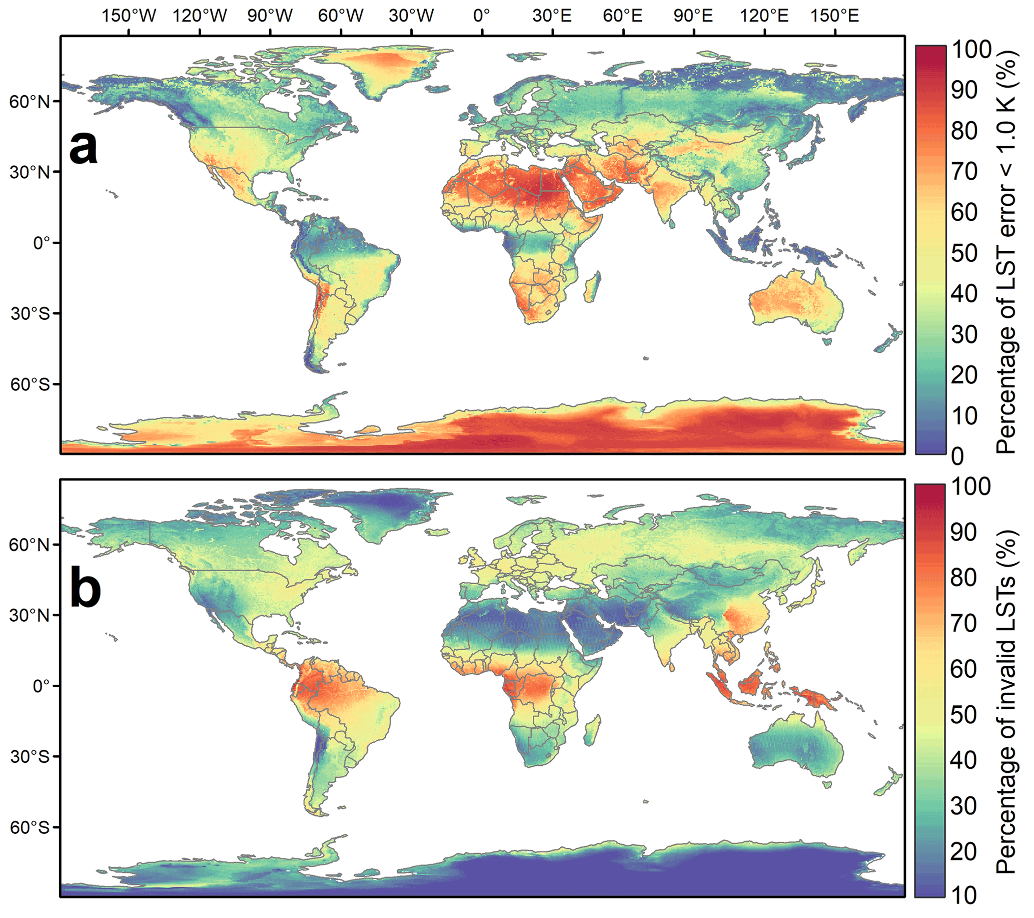
Figure A2 Uncertainties of the downloaded MODIS MXD11C1 V6 LSTs. Panel (a) shows the percentage of LSTs with a retrieval error less than 1.0 K, and panel (b) displays the percentage of invalid data (≈ clouds).

Appendix B: Mean absolute errors of T_{dm_IADTC} and T_{dm_OADTC} in Scenarios no. 1 and no. 3 at the site level

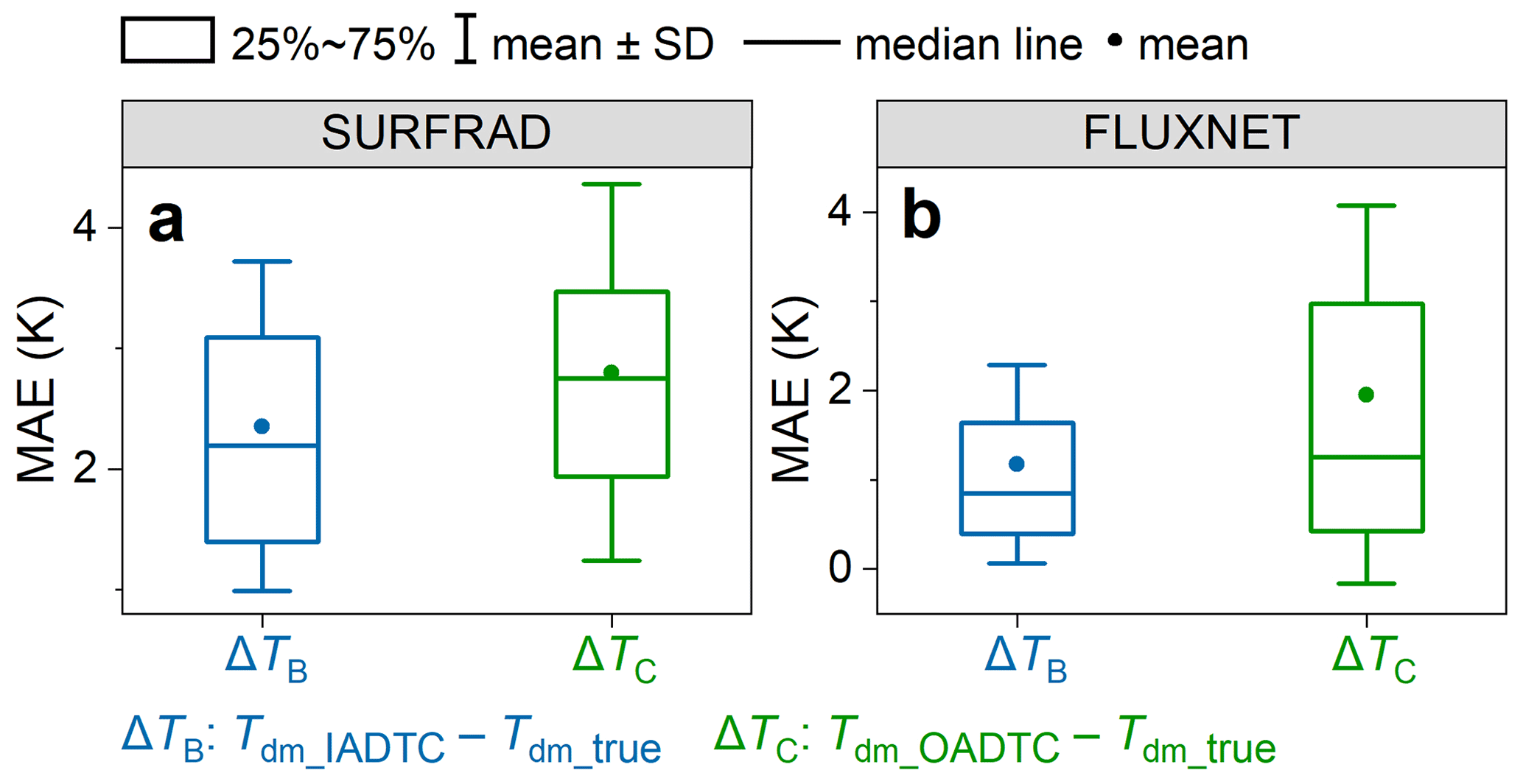
Figure B1 Box plots for the MAEs of the IADTC framework (T_{dm_ATC_DTC}) and the OADTC framework (T_{dm_OADTC}) under Scenarios no. 1 and no. 3. Panels (a) and (b) are for the SURFRAD and FLUXNET measurements, respectively.

Appendix C: Distribution of average sampling bias per season

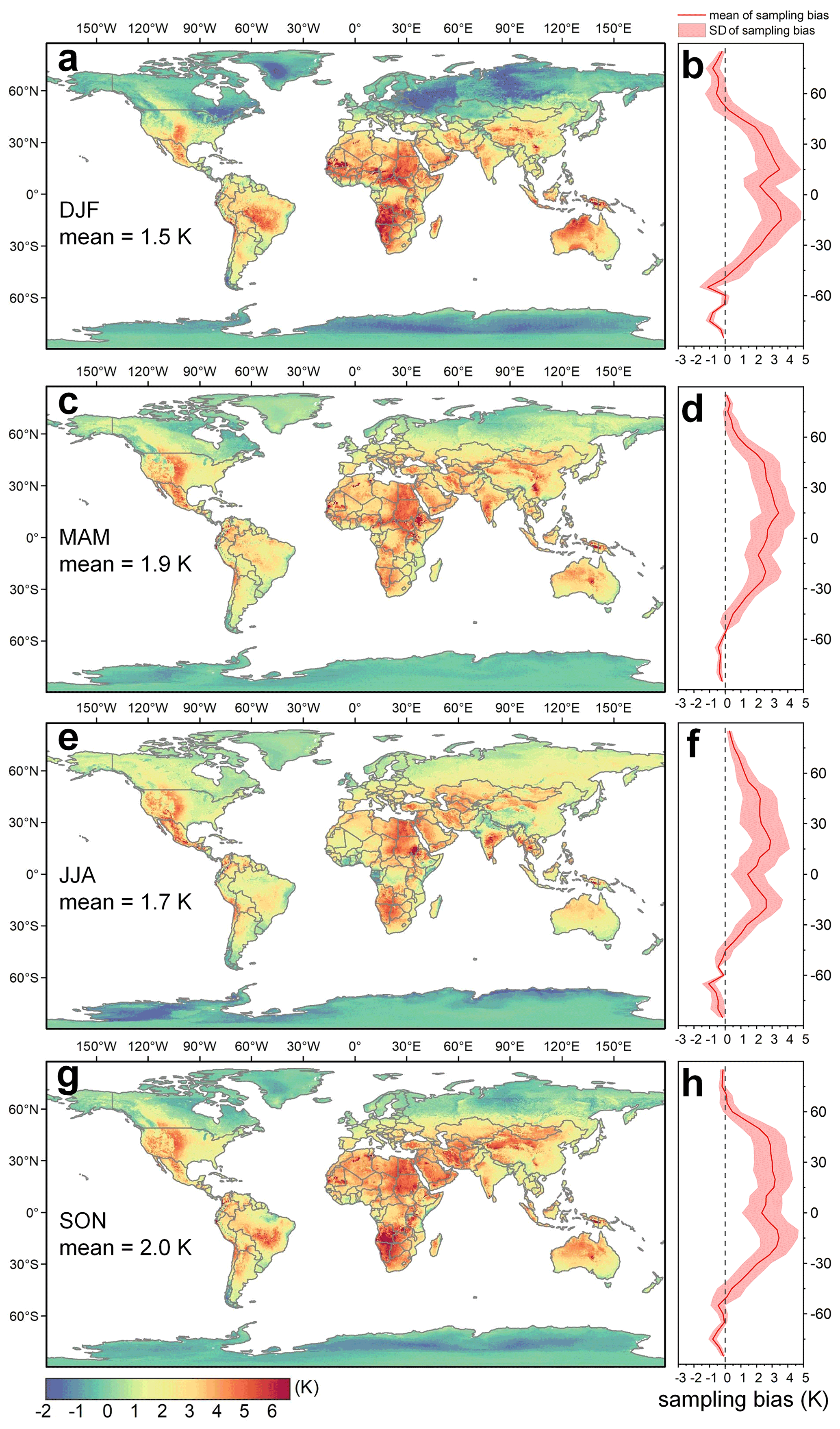
Figure C1 Average sampling bias ΔT_sb for indicated 3-month interval between 2003 and 2019. Panel (a) displays the ΔT_sb for December–January–February (DJF), and (b) displays the corresponding results averaged over 5^∘ longitudinal intervals. Similarly, (c) and (d), (e) and (f), and (g) and (h) display the corresponding results for March–April–May (MAM), June–July–August (JJA), and September–October–November (SON), respectively.

Appendix D: Nomenclature

Acronyms
ASTER	Advanced Spaceborne Thermal Emission and Reflection Radiometer
ATC	annual temperature cycle
AVHRR	Advanced Very High-Resolution Radiometer
BSV	barren sparse vegetation
CRO	croplands
DBF	deciduous broadleaf forests
DOY	day of year
DTC	diurnal temperature cycle
DTR	daily temperature range
EBF	evergreen broadleaf forests
ENF	evergreen needleleaf forests
GADTC	global daily mean LST product generated with the improved ADTC-based framework
GOES	Geostationary Operational Environmental Satellite
GRA	grasslands
IADTC	framework improved ADTC-based framework
IGBP	International Geosphere-Biosphere Programme
LST	land surface temperature
MAE	mean absolute error
MERRA-2	Modern-Era Retrospective analysis for Research and Applications version 2
MF	mixed forests
MODIS	Moderate-Resolution Imaging Spectroradiometer
MSG-SEVIRI	the Spinning Enhanced Visible and Infrared Imager onboard Meteosat Second Generation
OADTC framework	original ADTC-based framework
OSH	open shrublands
SAV	savannas
SAT	surface air temperature
SNO	snow and ice
SURFRAD	Surface Radiation Budget Network
WET	permanent wetlands
WSA	woody savannas
Symbol representation
DTRfour	diurnal temperature range calculated by the four LSTs which include the cloud-free
	LSTs and ATC-reconstructed LSTs
DTRDTC	diurnal temperature range calculated by the DTC model
ΔDTR	the difference between DTRDTC and DTRfour
Tdm	daily mean LST
Tdm_ATC_DTC	daily mean LST calculated by frequently sampling diurnal LST dynamics modeled by
	DTC model with cloud-free LST observations and under-cloud LSTs reconstructed by ATC model
Tdm_ATC_four	daily mean LST calculated by averaging cloud-free LST observations and under-cloud
	LSTs reconstructed by ATC model
Tdm_cloud_free	daily mean LST calculated by averaging cloud-free LST observations
Tdm_IADTC	daily mean LST estimated with the IADTC framework
Tdm_OADTC	daily mean LST estimated with the OADTC framework
Tdm_true	true daily mean LST for validation
Tin_ATC	instantaneous under-cloud LSTs reconstructed by ATC model
Tin_ATC_DTC	diurnal LST dynamics modeled by DTC model with cloud-free LST observations and
	under-cloud LSTs reconstructed by ATC model
Tin_cloud_free	instantaneous cloud-free LST observations
Tin_obs	hourly LST observations
Tin_under_cloud	instantaneous under-cloud LST observations
ΔTsb	sampling bias