the Creative Commons Attribution 4.0 License.
the Creative Commons Attribution 4.0 License.
 | 28 Jan 2022
Improved BEC SMOS Arctic Sea Surface Salinity product v3.1
Justino Martínez
Antonio Turiel
Verónica González-Gambau
Marta Umbert
Nina Hoareau
Cristina González-Haro
Estrella Olmedo
Manuel Arias
Rafael Catany
Laurent Bertino
Roshin P. Raj
Jiping Xie
Roberto Sabia
Diego Fernández
Measuring salinity from space is challenging since the sensitivity of the brightness temperature (TB) to sea surface salinity (SSS) is low (about 0.5 K psu−1), while the SSS range in the open ocean is narrow (about 5 psu, if river discharge areas are not considered). This translates into a high accuracy requirement of the radiometer (about 2–3 K). Moreover, the sensitivity of the TB to SSS at cold waters is even lower (0.3 K psu−1), making the retrieval of the SSS in the cold waters even more challenging. Due to this limitation, the ESA launched a specific initiative in 2019, the Arctic+Salinity project (AO/1-9158/18/I-BG), to produce an enhanced Arctic SSS product with better quality and resolution than the available products. This paper presents the methodologies used to produce the new enhanced Arctic SMOS SSS product (Martínez et al., 2019) . The product consists of 9 d averaged maps in an EASE 2.0 grid of 25 km. The product is freely distributed from the Barcelona Expert Center (BEC, http://bec.icm.csic.es/, last access: 25 January 2022) with the DOI number https://doi.org/10.20350/digitalCSIC/12620 (Martínez et al., 2019). The major change in this new product is its improvement of the effective spatial resolution that permits better monitoring of the mesoscale structures (larger than 50 km), which benefits the river discharge monitoring.
Please read the corrigendum first before continuing.
-
Notice on corrigendum
The requested paper has a corresponding corrigendum published. Please read the corrigendum first before downloading the article.
-
Article
(2049 KB)
-
The requested paper has a corresponding corrigendum published. Please read the corrigendum first before downloading the article.
- Article
(2049 KB) - Full-text XML
- Corrigendum
- BibTeX
- EndNote


Changes in the Arctic Ocean freshwater distribution may be linked to changes in the thermohaline circulation, which in turn may have implications for the global climate (Manabe, 1995). Thus, it is critical to understand the mechanisms of freshwater exchanges between the Arctic and the global ocean.
However, the number of in situ surface salinity measurements is, therefore, very scarce, and especially in the central Arctic Ocean, since it is a region with extreme weather conditions, and sea ice forces are strong enough to destroy the in situ measurement infrastructures (like Argo floats, moorings, or gliders).
The use of L-band radiometry to fill the observational salinity gaps at high latitudes could be very useful to better monitor the observed changes in the freshwater fluxes (Fournier et al., 2020). In 2009, the ESA SMOS (Soil Moisture Ocean Salinity) satellite mission was launched (Kerr et al., 2010). It was the first satellite carrying an L-band radiometer enabling the measurement of the ocean sea surface salinity.
The SMOS frequency band (1.43 GHz, L-band) is an optimum band to measure salinity, since this electromagnetic region is protected against human electromagnetic emissions, while the sensitivity to salinity is high.
The SMOS standard sea surface salinity (SSS) retrieval algorithm (Font et al., 2010; Mecklenburg et al., 2009; Olmedo et al., 2021), as well as the algorithms used for SSS retrieval from Aquarius and SMAP data (Tang et al., 2017, 2020), in general provide good estimates of SSS in the open ocean and within the tropical and midlatitudes (Reul et al., 2020).
However, SSS retrievals from the current operating L-band radiometer satellites present serious problems at high latitudes.
-
Low sensitivity of brightness temperatures (TB) to salinity in cold waters. Whilst the sensitivity to salinity is high at the L-band, the sensitivity decreases rapidly in cold waters. As shown in Yueh et al. (2001), such sensitivity drops from 0.5 to 0.3 K psu−1, when sea surface temperature (SST) decreases from 15 to 5 ∘C. Therefore, the errors of the SSS in cold waters are larger than in temperate seas.
-
Land–sea contamination (LSC) and ice–sea contamination (ISC). Sharp transitions of TB values between land and sea, or ice and sea, induce contamination of the signal, which is especially important (both in amplitude and spatial range) in the case of SMOS, due to the large footprint on the ground. Despite this instrumental characteristic, it is also present in SMAP and its predecessor, Aquarius. In the case of SMOS, this type of contamination has an impact on ocean observations very far from the coast and the ice.
-
Lack of in situ measurements. The limited number of in situ measurements of SSS in the Arctic is a major limitation, for the validation, since measurements are not evenly distributed, so that some regions have a clear lack of them.
In the framework of the ESA project Arctic+Salinity (AO/1-9158/18/I-BG), 9 years (2011–2019) of an enhanced SMOS SSS product have been produced. BEC distributes Level 2 maps and Level 3 maps of 3, 9, and 18 d in an EASE 2.0 grid of 25 km. The major changes in the algorithms have been focused on improving the effective spatial and temporal resolution of the product, allowing better monitoring of the mesoscale structures and the river discharges. The algorithms used for the generation of this new product are detailed in the Algorithm Theoretical Baseline Document (ATBD) of the Arctic+Salinity product (Martínez et al., 2020).
This paper describes the datasets (Sect. 1.1) used for the generation of the product and its validation, the algorithms developed to generate the new product (Sect. 2) and the validation performed to assess the quality of the product, namely (i) comparison with in situ measurements, (ii) spectral analysis, and (iii) error characterization by using triple collocation with SMAP data (Sect. 3).
1.1 Datasets
1.1.1 SMOS brightness temperatures
The computation of TB starts from the ESA Level 1B v620 product. This dataset is freely available with prior registration at https://earth.esa.int/eogateway/missions/smos/data (last access: 25 January 2022).
L1B product contains TB Fourier components arranged in a time-ordered way according to the integration time.
1.1.2 Auxiliary data used in the salinity retrieval
Geophysical variables from the European Centre for Medium-Range Weather Forecasts (ECMWF)
The auxiliary information is provided by ECMWF (Sabater and De Rosnay, 2010) collocated in time and space with each SMOS orbit. The data are provided in the Icosahedral Snyder Equal Area 4H9 (ISEA 4H9) grid (Matos et al., 2004). We use a nearest-neighbor interpolation to get the values in the custom TB grid.
Sea ice concentration from Ocean and Sea Ice Satellite Application Facility (OSISAF)
The sea ice concentration (SIC) product from OSISAF is used to discard the grid points contaminated by sea ice. We use SIC product version OSI-450 and OSI-430-b (Lavergne et al., 2019) developed and processed in the context of the OSISAF; https://osi-saf.eumetsat.int, last access: 25 January 2022) of the European Organisation for the Exploitation of Meteorological Satellites (EUMETSAT) and the Climate Change Initiative (CCI) program of the European Space Agency (ESA). The grid of these products is the EASE-Grid 2.0 with a spatial resolution of 25 km.
1.1.3 Annual SSS and SST climatology
The World Ocean Atlas 2018 (WOA 2018 – A5B7) annual SSS and SST climatologies at 0.25∘ × 0.25∘ spatial resolution (Zweng et al., 2018) are used in the inversion algorithm. The SSS and SST are used as inputs of the Meissner and Wentz dielectric constant model to obtain TB (Meissner and Wentz, 2004, 2012). The obtained TB value is considered the reference value to perform the spatial bias correction of the measured TB. WOA 2018 – A5B7 (generated from measurements of the 2005–2017 period) has been used to be consistent as much as possible with the SMOS life period.
1.1.4 Global Ocean Forecasting System
The Global Ocean Forecasting System (GOFS) 3.1 (HYbrid Coordinate Ocean Model, HYCOM + Navy Coupled Ocean Data Assimilation, NCODA) sea surface salinity product is used as the reference to perform the temporal correction. The spatial resolution of this product is 0.08∘ in longitude and 0.04∘ in latitude for polar regions and corresponds to the GLBv0.08 grid (Cummings, 2005; Cummings and Smedstad, 2013). The data can be downloaded from https://www.hycom.org/data/glbv0pt08 (last access: 25 January 2022).
1.1.5 ARGO dataset
ARGO float data (Argo, 2018) are commonly used for the validation of SSS from SMOS and SMAP data (Tang et al., 2017; Olmedo et al., 2021). However, this is complicated in the Arctic region. ARGO data are very scarce and Argo profilers are concentrated in the Atlantic region (due to bathymetry and geographical restriction of ocean circulation), providing a biased sample of the mean SSS in the Arctic. There is a lack of Argo profilers in the Bering, Beaufort, East Siberian, Laptev, Kara, Barents, and North seas and also in the Hudson and Baffin bays (see Fig. 7).
The following quality control over the values of Argo SSS is used: the cut-off depth for Argo profiles is taken between 5 and 10 m. Profiles included in the grey list (i.e., floats which may have problems with one or more sensors) are discarded. Argo float profiles with anomalies larger than 10 ∘C in temperature or 5 psu in salinity when compared to WOA 2013 are discarded. Finally, only profiles having a temperature between −2.5 and 40 ∘C and salinity between 2 and 41 psu close to the surface are used.
1.1.6 Tara OCEANS (2009–2013) expedition dataset
The Tara OCEANS (2009–2013) expedition collected SST and SSS at 3 m depth during the whole cruise between 2009 and 2013 all around the world thanks to the thermosalinograph (TSG) Seabird SB45 and a temperature sensor (SBE38) that was on board its research vessel, Tara. The Arctic Ocean data correspond to the period of June to October 2013. Hereafter, this dataset is referred to as Tara SSS (Reverdin et al., 2014).
1.1.7 JPL SMAP dataset
Level 3 SSS maps, version 4.2, provided by the Jet Propulsion Laboratory (JPL) (from https://podaac.jpl.nasa.gov/dataset/SMAP_JPL_L3_SSS_CAP_8DAY-RUNNINGMEAN_V42, last access: 25 January 2022) are used for the quality assessment on the triple collocation analysis.
The generation of the improved and higher-spatial-resolution salinity maps has followed several steps which are described below. A scheme of the whole algorithm is shown in Fig. 1 (for more details, the reader is referred to the ATBD of the Arctic+ project; Martínez et al., 2020).
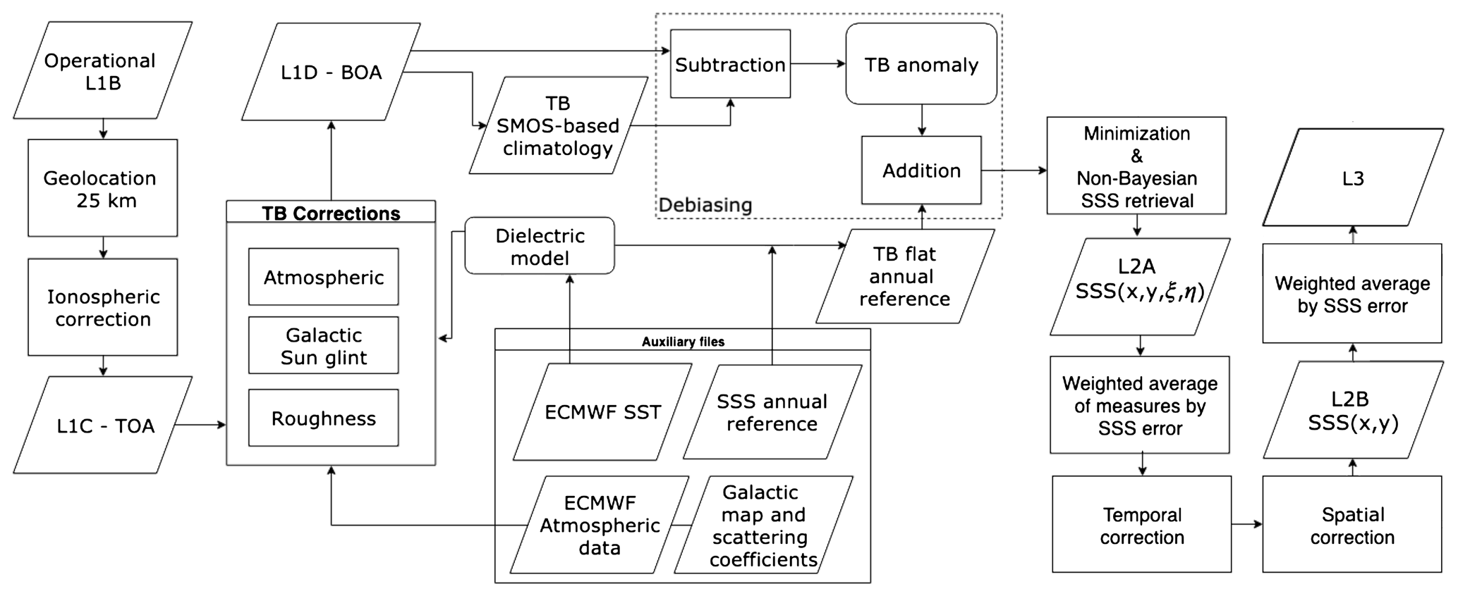
Figure 1General block diagram for Arctic SSS retrieval. The debiased non-Bayesian method was applied as part of the algorithm, but debiasing was done in TB rather than in SSS.
2.1 Geolocation and projection of the brightness temperatures
We use the ESA Earth Explorer Mission CFI propagation libraries v. 3.7.4 (ESA, 2014) to geolocalize the SMOS TB measurements. The geographic coordinates (longitude and latitude) are transformed to plane coordinates by means of the Lambert azimuthal equal-area map projection (LAEA) (Snyder, 1987).
As in the standard procedure (Anterrieu et al., 2002), we apply a Blackman window to the Fourier components in order to reduce the Gibbs-like contamination. The TB is obtained by applying an inverse Fourier transformation to the resulting TB coefficients. The antenna hexagonal grid in which the TB image is reconstructed contains 64×64 points (instead of 128 used in the standard SMOS L1 processor). This resolution in the antenna level results in 4096 grid points being enough to provide the TB values because the number of visibilities from which snapshots are derived by a linear transformation is 2791. This choice allows us to reduce the computational time without loss of information/resolution. The areas of the field of view (FOV) containing aliases between different regions of the Earth are discarded. Once all the geolocation magnitudes have been computed and the measured TB(ξi,ηi) values are known in all 64×64 FOV points, the Earth grid is generated and the points of this grid are retroprojected up to the SMOS antenna coordinate reference system for each SMOS snapshot. In this v3.1 product, we have computed the TB values directly in the final grid of the salinity map products. This choice has been made to keep the maximum information of the salinity gradients without losing resolution due to interpolation errors.
2.2 Computation of the brightness temperatures at the ocean surface
The TB transformation from the top of the atmosphere (TOA) (see the previous section) to the bottom of the atmosphere (BOA) is similar to the one performed in the operational SMOS level 2 processor chain (more details are described in ICM-CSIC et al., 2016). The measured TB by SMOS is the result of different contributions (Zine et al., 2008): sea emission, atmosphere emission contribution, galactic contribution, and sun glint.
The galactic and sun glint contributions are computed following the models described in Tenerelli et al. (2008) and Reul et al. (2007), respectively. We use the roughness model developed by BEC (Guimbard et al., 2012). The auxiliary data provided by ECMWF are collocated with SMOS measures and used to evaluate the models. Finally, we compute the TB corresponding to the flat sea contribution ( and ) by subtracting the rest of the contributions. The polarizations of the SMOS TB values are affected by the ionosphere, and they can be corrected following Zine et al. (2008). Nevertheless, the ionosphere produces a rotation between the TB polarizations, leaving the first Stokes parameter unaltered (), the parameter used to perform the TB inversion.
2.3 Debiasing
The debiased non-Bayesian retrieval method was introduced in Olmedo et al. (2017) to retrieve salinity from SMOS TB. Salinity retrieval is performed by means of a minimization of the difference between the measured first Stokes parameter and the modeled one. This minimization follows a non-Bayesian scheme; i.e., a SSS value is retrieved for each TB measurement. The new Arctic salinity product also retrieves salinity using a non-Bayesian scheme but introducing important changes.
The SSS debiasing approach employed in the previous version of the BEC Arctic SMOS SSS product (v2.0, Olmedo et al., 2018) started from a long-term time series (8 years) of SSS retrievals. These SSS retrievals were grouped according to their geographical location, incidence angle, distance to the center of the swath (across-track distance), and satellite overpass direction. These salinity values were accumulated in classes for each group, obtaining the discrete salinity distribution function for each one. The characteristic value of these distributions can be considered the SMOS-based salinity climatology. The mean around the mode of each distribution was chosen as its characteristic value. To mitigate the local time-independent biases, the corresponding SMOS climatology is subtracted from each measured SSS value and replaced by an annual SSS reference. World Atlas Ocean 2013 (WOA) (Zweng et al., 2013) was the reference of choice for v2.0. This method mitigates biases like those caused by land–sea contamination or permanent radio frequency interference (RFI) sources.
In this work, we aim at improving the algorithm in two specific points. First, the non-homogeneous division of the antenna FOV into groups of incidence angles and across-track distance derives into different statistic representativeness for different points of the antenna, providing a non-optimal resolution of the final climatological salinity product. This has been improved by introducing a homogeneous discretization of the extended alias-free field of view (EAF-FOV) in ξη coordinates. Secondly, the non-linearity of the L-band dielectric models at very low salinity ranges amplifies the errors of the retrievals at low salinity values. Since the retrieval procedure propagates systematic errors from the TB value to the resulting SSS, the debiasing is applied at the TB level and not at the SSS level, so as to mitigate as much as possible these effects (more details can be found in Martínez et al., 2020).
The interferometric nature of SMOS divides the SMOS antenna FOV into a hexagonal grid. Accordingly, the antenna FOV has been homogeneously divided into hexagonal cells that cover the same antenna area. To ensure that a number of measurements large enough are accumulated by each hexagonal cell to compute a reliable SMOS-based climatology, each cell contains seven points of the original 64×64 FOV grid.
To perform the spatial bias correction, the measured first Stokes parameter is grouped into discrete distributions according to the antenna cell in which it has been acquired, its geographical location on the Earth, and the satellite flight direction. Thereby, the SMOS-based climatology is subtracted from the individual measures of the first Stokes parameter, and the annual reference is added to it. No brightness temperature exists from World Ocean Atlas, so it is necessary to compute it starting from WOA 2018 SSS and SST (Zweng et al., 2018) using the Meissner and Wentz dielectric model.
2.3.1 SMOS-based climatology
The SMOS-based climatology has been computed using the SMOS TB data from the 2013–2019 period (both included). We discarded the years 2011 and 2012 because of the strong affectation of RFI in the earlier years of the mission.
The SMOS-based climatology is performed by computing the distribution of the first Stokes parameter separately for ascending and descending orbits. The histograms are created by accumulating valid measures in bins of 1 K for each 25 km EASE-Grid 2.0 North grid point (x and y coordinates) and FOV coordinates (ξ and η coordinates). Only latitudes beyond 50∘ N are considered.
We apply the following filtering criteria over I before computing the climatology.
-
Only measurements in the range 75 K K are considered.
-
Measurements acquired with ECMWF SIC values larger than 0.05 are discarded.
-
The Tukey (1977) rule is used to detect outliers. Then, measures Δ accomplishing one of these conditions,
are considered outliers. Here and Q1 and Q3 are the first and third quartiles, respectively. Outlier detection is implemented in two stages.
-
We compute the linear regression from all the TB(θ) measures for a given geographical point obtained at different incidence angles (θ) in a given orbit. Outliers are detected by computing the difference between this linear regression and each individual measurement (Δ).
-
The rule is also applied for each distribution.
-
Once the valid measurements are selected, for each acquisition condition , with d the orbit direction, we accumulate the TB measurements () acquired under γ conditions in Iflat(γ). The histograms are created adding only valid measurements in bins of 1 K for each 25 km EASE-Grid 2.0 North grid point (x and y coordinates) including the measures collected in a 75×75 km square. The measurements are grouped for each FOV cell composed of seven unshared ξ and η coordinates.
Then, for each γ, we compute the following statistical parameters: frequency, mean, median, interquartile range, and the second, third, and fourth central moments. The representative value used afterwards for the debiasing, namely the SMOS-based climatology, is assumed, as in the previous version of the debiasing method, to be the mean around 1 standard deviation from the mode of the Iflat(γ).
2.4 Inversion
Once the systematic errors of the measured flat sea are corrected, the SSS retrieval can be performed by using a dielectric constant model. The flat sea emissivity is described by Fresnel reflection law that is a function of the incidence angle of the radiation θ and the dielectric coefficient ε, which depends on the SST, the frequency, and the conductivity, which in turn depends on the salinity.
In the L-band range, the more common dielectric constant models used are the Klein and Swift model (KS) (Klein and Swift, 1977) and Meissner and Wentz model (MW) (Meissner and Wentz, 2004, 2012). These dielectric models are based on a Debye relaxation law (Debye, 1929) with a conductivity term. The MW model interpolates the dielectric constant as a function of salinity between 0 and 40 psu and provides values for the ocean surface temperature between −2 and 29 ∘C. The KS model was adjusted using a discrete set of measures at 5, 10, 20, and 30 ∘C, and it is reported by authors to be valid in the range of 4–35 psu. However, the KS model has a very problematic behavior below 5 ∘C (Zhou et al., 2017; Dinnat et al., 2019), so we have used the MW model to derive the high-latitude SSS. It has been reported that the SST-dependent bias in the retrieved SSS in cold waters could be mainly due to deficiencies in the sea water dielectric constant models (Dinnat et al., 2019). The MW model is not free from this pathology, but the large errors that the KS model produces below 5 ∘C reinforce the choice of MW as the sea water dielectric model.
We obtain the salinity value by minimizing the following cost function:
with the first Stokes parameter described by the models. We use the Newton–Raphson method (Press et al., 1992) to find the SSS value that minimizes the equation F.
2.4.1 TB filtering approach
We apply the following filtering criteria before the inversion.
-
Values of too close to the belts and suspenders (closer than 0.025 antenna units) are discarded (see Fig. 2).
-
Points affected by Sun tails or reflected Sun circle are also discarded.
-
The values considered outliers during the SMOS-based climatology computation (Sect. 2.3.1) are discarded as well.
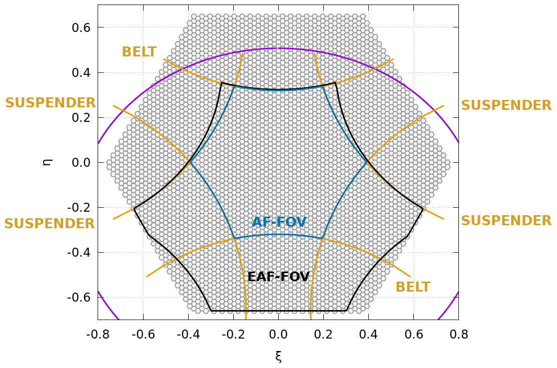
Figure 2The 64×64 SMOS hexagonal field of view. Purple lines indicate the Earth limit; beyond this limit the FOV points contain sky TB. Blue and black lines encircle the AF-FOV and EAF-FOV, respectively. Points in the horizontal yellow lines are known as belts whereas suspenders are the points included in the vertical yellow lines. Belts and suspenders are points of transition between the free-alias zone and zones affected by Earth–sky aliases or between zones affected by different Earth–sky alias; therefore the measures are expected to be somewhat degraded over there.
Additionally, TB values are discarded if the SMOS-based climatology used for its bias correction is considered a moderately non-normal distribution (kurtosis and skewness conditions according to West et al., 1995), if climatology has been computed using a low number of measures, or if the standard deviation of the climatological distribution is too high close to the coast (suspicion of residual land–sea or persistent RFI contamination). These conditions are summarized in the following rules.
-
The minimum number of measures to create the SMOS-based climatology must be 100.
-
The absolute value of kurtosis must be less than 7.
-
The absolute value of skewness must be less than 2.
-
For points located less than 100 km from the coast, only those having a standard deviation less than 8 K are taken into account.
To ensure the minimum ice–sea contamination, all points having SIC >0 according to Sea Ice Climate Change Initiative products OSI-450 and OSI-430-b (Lavergne et al., 2019) are not included in the minimization process. The distance to the ice edge (defined by the line SIC =0) is also stored with the same purpose (minimizing the ice–sea contamination by avoiding the points too close to the ice in the L3 map generation).
2.4.2 Minimization and error propagation
Once we have the valid values (passed the filtering process), we perform the debiasing method. This method consists in subtracting the SMOS climatologic value from the and adding the WOA-derived climatological value. We apply the following convergence criteria in the iterative scheme.
-
The change in salinity values between two consecutive iterations is less than 0.001.
-
The percentage of variation in the cost function between consecutive steps is less than 1.
-
The above two conditions are accomplished during five consecutive iterations to avoid oscillatory solutions.
-
The above condition is accomplished in fewer than 150 iterations.
The propagation of the TB radiometric error to salinity is made by performing the minimization of two additional quantities.
Here σ[H,V] is the radiometric accuracy of . Then, the salinity error is computed from the following equation:
where SSSmeas+ and SSSmeas− are obtained by the inversion of and , respectively.
2.4.3 SSS filtering approach
Once each orbit has been processed, we perform the inversion using the mentioned MW dielectric model to create orbits that contain one salinity value for each measured TB. At this level, we obtain for each location as many salinity values as measurements have been inverted. Thus, the salinity is a function of the incidence angle. To create this product we apply the following filtering criteria.
-
and are discarded.
-
In the case of , we discard the retrieval when .
-
In the case of , we discard the retrieval when . We relax the criteria in this case to better capture the river discharges and melting episodes, which are not well described in WOA 2018.
2.5 Generation of SSS satellite overpasses
Prior to the L3 map generation, we create the L2B product. The L2B orbits provide salinity values independent from the antenna point acquisition and are generated from L2A snapshots by weighted averaging of all the measures obtained for a given grid point. Outlier detection is performed in a similar way as it was applied to TB: a linear regression is performed from all the incidence-angle-sorted SSS values of the same orbit obtained for a given geographical point. The outliers are detected, according to the Tukey (1977) rule, from the difference between this linear regression and each individual measure. L2B SSS values are only computed for those grid points containing more than 12 unfiltered L2A retrieved SSS values.
Assuming the weight function as the inverse of the squared error of each L2A SSS measure, we ensure that the measures coming from TB having a high radiometric error will have a small influence in the obtained value for SSS at the L2B level. This procedure will help, also, to mitigate the effect of scenes contaminated by RFI. Therefore, the average of all of the SSS retrievals for a given location is weighted in the following approach:
where the weight function is given by
where is given by expression (3). Therefore, the error of each L2B salinity value is given by the expression
2.6 Temporal bias correction
The TB debiasing procedure only accounts for the spatial biases, so that a temporal correction is also required. The correction implemented in the previous version operates over L3 maps and is based on Argo profiles. The median of the differences between the collocated L3 SSS and the Argo profiles available for the 9 d period of each map is removed from the corresponding 9 d SSS map. Since we also need to perform a time correction on L2 SSS orbits, and the amount of ARGO data available for each orbit is insufficient, we propose performing the temporal bias corrections using the Global Ocean Forecasting System (GOFS) 3.1 (HYCOM + NCODA) as reference. The correction is based on the iterative scheme presented in Fig. 3 and detailed as follows.
-
Step 1. We start subtracting 12 psu from all SSS (grid point level) retrievals. This intends to reduce the number of iterations in the loop and to improve the convergence. The value of 12 psu has been obtained as the better one after several retrieval processings.
-
Step 2. We apply the filtering criteria described in Sect. 2.4.3, and we average the corresponding filtered SSS retrievals in each grid point to generate the satellite overpass (as described in Sect. 2.5)
-
Step 3. We update the temporal correction value with the mean difference between each value of the SSS (at orbital level) and the collocated HYCOM salinity.
-
Step 4. We add this temporal correction to each at the snapshot level.
-
We repeat steps 2–4 until the difference between two consecutive corrections is lower than 0.01 psu.
Only orbits providing at least 50 common grid points with HYCOM are considered. Due to the fact that HYCOM provides too salty values in the river mouths, only grid points having a retrieved salinity value above 25 psu and an error below 2.5 psu are considered to compute the temporal correction.
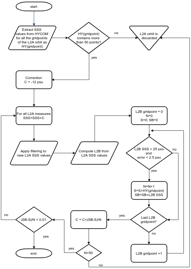
Figure 3Scheme of the iterative procedure used to correct the temporal salinity bias on level 2.
2.7 Correction of the residual spatial bias
As it has been described in Sect. 2.3, the debiasing method is based on the substitution of the SMOS-based TB climatology by the SSS reference from WOA 2018 (Zweng et al., 2018). With that method, a first-order spatial correction is performed.
After the debiasing method, the average salinity obtained for the period used to compute the SMOS-based climatology (years 2013–2019) should have a spatial distribution very close to the reference used to carry out the debiasing (WOA2018). However, the difference between the weighted average of all SSS orbits from the years 2013 to 2019 and the averaged SSS from WOA is not close to zero, and significant differences are observed. The weighted average of all L2B orbits in the 2013–2019 period minus the value provided by WOA ranges between −10 and 10 psu but mainly between −2 and 2 psu. The values differ a lot between the Arctic zones, being smaller in the open ocean and larger in the North Sea (negative), the Beaufort Sea (positive), and the East Siberian Sea (positive).
The cause of the differences between ascending and descending passes is mainly linked to the different performances of the ascending and descending debiasing. Depending on the coast orientation, a given point can be affected by land–sea contamination in ascending or descending passes differently, hence requiring a different correction, too. A similar behavior is observed with ice–sea contamination and when RFIs are present.
The first Stokes distributions provided by SMOS have generally positive skewness. This means that its representative (the mean around the mode) at each geographical point generally does not match with the mean of the distribution. On the other hand, the WOA 2018 salinity is obtained through an objective analysis scheme using a correction factor given by a weighted average of the in situ measurements in a given limited region (Zweng et al., 2018, Sect. 3.2), therefore assuming Gaussianity in this region. The substitution of the SMOS-based climatology by the TB reference obtained from WOA 2018 salinity introduces inaccuracies due to the skewness and other second-order statistical properties of the SMOS measurements.
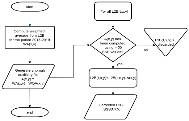
In order to mitigate this residual spatial bias, we compute an anomaly spatial map by applying the following algorithm to all the L2B orbits in the period 2013–2019 (shown in Fig. 4).
-
We compute the difference between SMOS overpass salinities and the ones provided by WOA 2018.
-
We generate two anomaly files: one for ascending and one for descending passes (they show differences of up to ±1.2 psu).
After the creation of these two anomaly maps, every L2B salinity value is corrected by subtracting this spatial anomaly. The salinity values corresponding to geographical points where the anomaly was computed using fewer than 50 collocations are discarded.
2.8 Generation of L3 SSS maps
L3 maps are generated daily for 9 d periods. Each map is obtained by a weighted average of all the SSS values in all the overpasses of the 9 d period. Each L2B salinity value is weighted according to its salinity error as described in Sect. 2.4.2. To minimize ice–sea contamination and land–sea contamination, the L2B points closer than 35 km to the ice edge or coastline are not considered during the process of L3 map creation.
Figures 5 and 6 show an example of the resulting 9 d L3 salinity maps (Fig. 5a) and the salinity error (Fig. 5b) derived from the radiometric uncertainty.
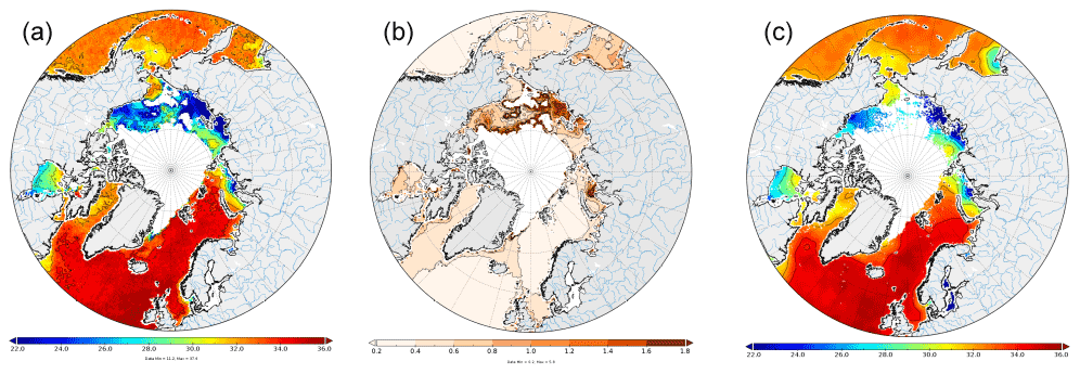
Figure 5(a) Arctic+ v3.1 9 d map of the period 11–19 August 2012. (b) Salinity error derived from the radiometric error. (c) Arctic+ v2.0 9 d map of the period 11–19 August 2012. A section of this map from the Barents Sea to the East Siberian Sea is shown in Fig. 6.
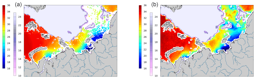
Figure 6(a) Detail of the Arctic+ v3.1 product from Fig. 5 together with the minimum Sea Ice concentration provided by OSI SAF for the period 11–19 August 2012. (b) Same region but for Arctic+v2.0. The right color bar indicates Sea Ice concentration whereas the left color bar indicates salinity.
Figures 5 and 6 show that the Arctic+ v3.1 product has greater coverage and gradient detail than the previous BEC Arctic v2.0 product.
The validation of the product is done using different in situ measurements; the results are described in detail in the Product Validation Report (Arias et al., 2020) that can be found on the project web page (https://arcticsalinity.argans.co.uk/documentation/, last access: 25 January 2022).
We recall some important aspects of this product and its validation procedure.
-
The validation in the Arctic region is rather complex due to the heterogeneity of the in situ datasets, with a lack of temporal or spatial synopticity. Some of the sources only represent specific regions, with the risk of inducing bias by spatial selection when assessing the product entirely. Others cover a larger spatial representation; however, a lack of a proper temporal variability still remains. None of the datasets used can describe both aspects simultaneously; thus the validation requires an exhaustive analysis of the results to assess the quality of the product.
-
The Arctic+ SSS v3.1 product introduces an improvement in the number of SSS retrievals obtained from SMOS TB for the Arctic region (as shown in Figs. 5 and 6). This represents a significant reduction of data gaps.
-
The new product benefits from a polar grid in EASE v2.0 format, which is a standard for the research and operations in the region, improving its usability.
-
The Arctic SSS+ v3.1 product has been built only using WOA 2018 and HYCOM model output, without using ARGO data.
-
The validation of the product using ARGO floats in the Arctic is only valid for the Greenland and Norwegian seas, where the Argo floats are present. However, a comparison with punctual measurements can not be used to evaluate the improved data coverage or the improved spatial resolution. Thus, the ARGO analysis can not be used alone to describe the quality of this product.
-
It is also important to highlight that, when inter-comparing satellite-based SSS products, there is a need to focus on the selected projections and grid. A fair set of metrics for inter-comparison is only possible over common points resolved at the same spatial scales. This means that the quality control for these products requires setting the products into the same spatial grids and projections. By not doing so, significant errors may be introduced artificially in the metrics, products may be penalized because of differences in the sampling strategies, and thus, the match-up databases do not yield the same points and hence information.
3.1 Comparison with ARGO data
Even though the ARGO floats are very scarce in the Arctic and are mainly in the Atlantic and Pacific regions (see Fig. 7), we have used Argo SSS data to assess the biases and the standard deviations of the errors of the new SSS products, but with the caution that this analysis is only valid for the region where Argo floats are present, and assuming that Argo values represent a ground truth for the whole pixel.
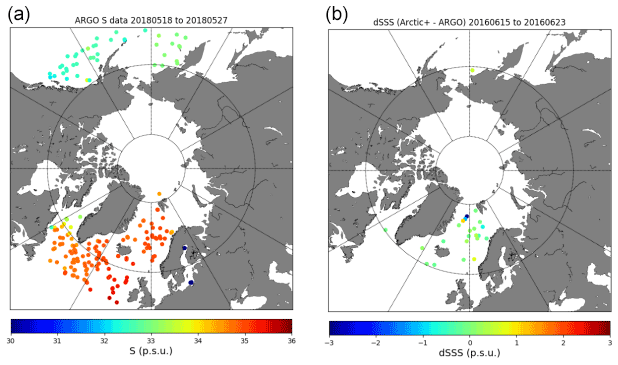
Figure 7(a) Example of total daily ARGO profiles matching the 9 d period associated with one Arctic+ v3.1 product (18 May 2018 to 27 May 2018). (b) Difference between SMOS SSS v3.1 and Argo data after selecting only valid match-ups for the product from 15 June 2018.
The methodology followed to perform the temporal and spatial collocation between the Argo SSS with the SSS maps is the following. For a given in situ point, the closest satellite point is searched both in time and in space, with a radius of 25 km from the in situ measurement and a maximum period of 9 d off in time. This strategy leads to some repetition in the use of the in situ data points for different maps, but never over the same daily product. This has been deemed as the most solid strategy, as it maximizes the quantity of in situ information to validate the satellite products.
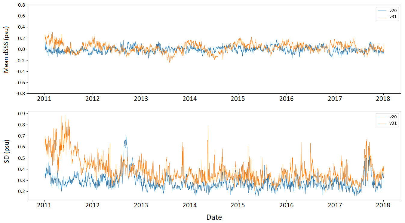
Figure 8Results of time series of metrics for bias and standard deviation per each 9 d map of the satellite-based products. The blue line corresponds to BEC v2.0 and the orange line to Arctic+ v3.1.
The statistics (bias and standard deviation) for the differences between Arctic+v3.1 and Arctic+v2.0 with respect to Argo measurements are shown in Fig. 8 for the period 2011 to 2017. The values for the complete period for v3.1 are mean=0.02, SD=0.39, RMSD=0.39, and correlation R=0.94. The values for v2.0 are , SD=0.28, RMSD=0.29, and correlation R=0.97. The standard deviation is larger than the previous BEC v2.0 product, but this is expected since the BEC Arctic v2.0 product was generated by performing objective analysis with correlation radii 321, 267, and 175 km (Olmedo et al., 2016). The large correlation radii produce a large smoothing effect, reducing the noise. However, the smoothing results in a reduction of the spatial resolution, which is significantly improved in the v3.1 product (see Sect. 3.3). The BEC v3.1 product, thus, contains more dynamic information than v2.0.
The degraded quality of data in the first 2 years (2011 and 2012) is due to a high RFI source located in Greenland that highly contaminated the measurements, and they could not be corrected during the processing step. Thus, we recommend the users avoid those two years of data. Later on, by the end of 2012, the main source of RFI was locked down, permitting higher-quality measurements (Oliva et al., 2016).
3.2 Comparison with Tara dataset
Tara salinity data present a large range in the spatial variability of salinity between 26 and 35 psu in the Arctic Ocean (see Fig. 9).
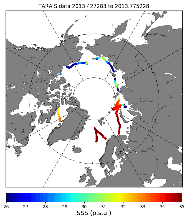
Figure 9Tara expedition TSG measured SSS values. Tara expedition circumnavigated the Arctic between June and October 2013 following a counterclockwise path. SSS data reveal the high spatial variability of SSS in the Arctic, as a result of the multiple sources of SSS variability (river tributaries, ice melting).
The mean, standard deviation (SD), root mean square difference (RMSD), and correlation (R) are computed for all the residuals of the collocated points between Tara and Arctic+ v3.1 (Table 1). To assess the quality of the Arctic+ v3.1 product over a specific region, a splitting of the Tara transect has been applied grouping data into sub-basins: the Norwegian Sea, Barents Sea, Kara Sea, Laptev Sea, East Siberian Sea, Chukchi Sea, Beaufort Sea, and Baffin Bay. The results are shown in Table 1.
Table 1Validation results of Arctic+ v3.1 and BEC v2.0 in Arctic sub-basins using Tara TSG data.
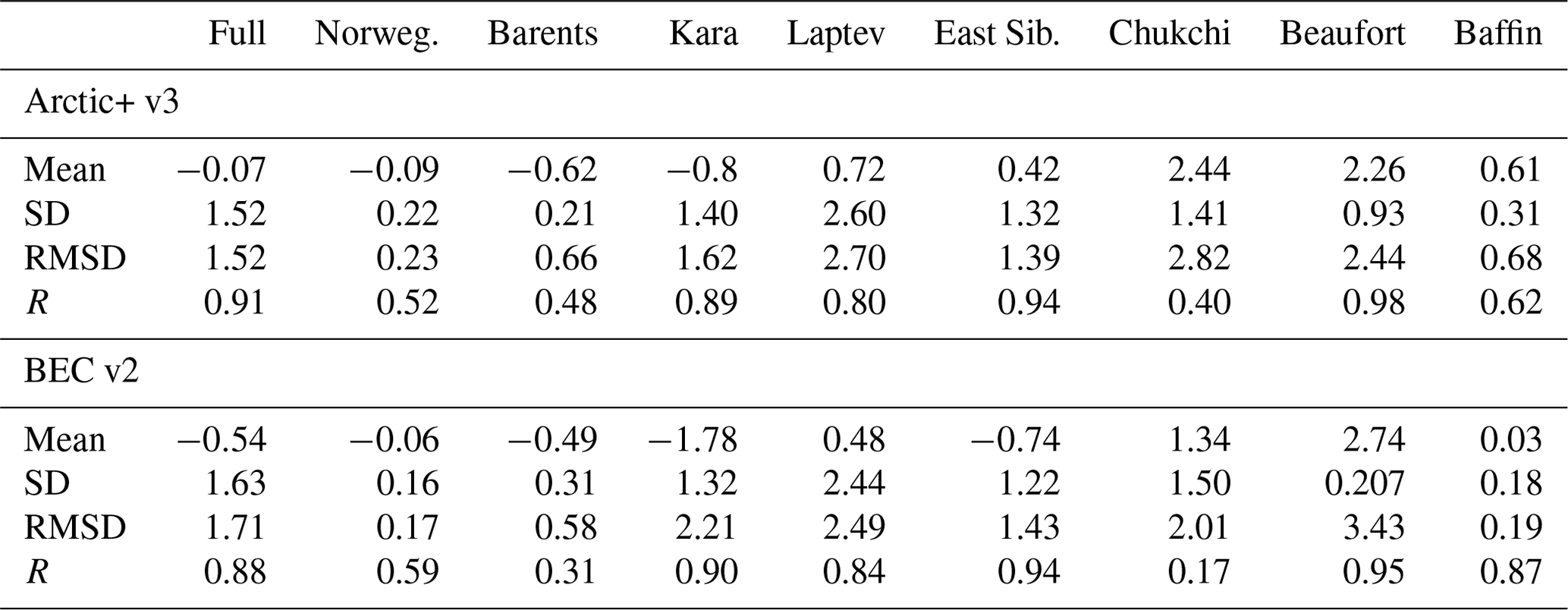
Matchups with Tara yield different results depending on the sub-basin. Arctic+ v3.1 products have a lower RMSD than BEC v2.0 product for three sub-basins (Kara, East Siberia and Beaufort seas) and also for the global value (see Product Validation Report; Arias et al., 2020).
Nevertheless, metrics with Tara are not simple to interpret due to the lack of synopticity in the dataset (acquired over a relatively long period of time, i.e., representing different observational conditions) and the lack of spatial homogeneity of the sampling, which explains the relatively large variability observed in the metrics for different sub-basins.
3.3 Error characterization by correlated triple collocation
Triple collocation (TC) is a method originally introduced by Stoffelen (1998) to provide estimates of the measurement error variances of three systems measuring the same variable at the same time. TC is based on the statistical relations between the measurement variances and covariances to deduce the error variances for each measurement. TC requires having a long enough series of collocated triplets of the measurements to obtain reasonable estimates of the second-order moments of those measurements.
Besides, it is usually required that the three measurement systems are completely independent, with different space-time acquisition scales, and thus the so-called representativity error must be properly accounted for (Stoffelen, 1998; Hoareau et al., 2018).
Recently, a variant of TC especially adapted to deal with remote sensing measurements has been introduced: the correlated triple collocation (CTC) (González-Gambau et al., 2020). When applying CTC, the data are assumed to have the same space-time sampling; that is, they represent the same spatial scale and timescale. In contrast with standard TC, it is assumed that two of the datasets can have correlated errors (for instance, they are derived from the same basic measurement system). In addition, and considering that remote sensing series are typically not too long, CTC is optimized to provide reasonably good estimates of the error variances even with a limited number of samples. With those conditions, CTC can be used to obtain maps of error variances of triples of remote sensing SSS maps and obtain, for example, a different map for every year.
We have applied the CTC, following González-Gambau et al. (2020), to characterize the SSS errors with 2016 data. We have taken three sets of collocated SSS maps: JPL SMAP v4.2 SSS, 8 d maps; BEC SMOS Arctic SSS v2.0, 9 d maps; and BEC SMOS Arctic+ v3.1, 9 d maps. We have considered the products reduced to the common resolution (that of BEC v2.0).

Figure 10Error standard deviations computed via correlated triple collocation for BEC SMOS Arctic SSS v2.0 (a), BEC SMOS Arctic SSS v3.1 (b), and JPL SMAP SSS v4.2 (c), for all the collocated maps in the year 2016.
The correlated triple collocation analysis helps to properly assess the differences existing between the derived satellite products. Figure 10 shows the estimated error standard deviation for each one of the three datasets. The differences between the products are shown in Fig. 11. Over the majority of the Arctic, BEC v3.1 has the smallest error, except in some specific regions where BEC v2.0 is better (Hudson Bay, east coast of Greenland, and Kara Sea). JPL 4.2 is the product with the greatest error in all cases.

Figure 11Difference between the error standard deviations of BEC SMOS SSS v2.0 (a) and of JPL SMAP SSS v4.2 (b) with BEC SMOS SSS v3.1 for the year 2016.
3.4 Spectral analysis
The analysis of spectral slopes permits us to obtain information about the effective spatial resolution of the different remote sensing datasets. Theoretical studies have reported that power density spectra (PDS) slopes are expected to range between −1 and −3, depending on the dynamical regime that drives the ocean (Blumen, 1978; Charney, 1978). Moreover, the presence of white noise makes the spectral slope tend to 0 (log PDS vs. log wavenumber bend and become horizontal at high wavenumbers). In contrast, when the spatial resolution of the data is oversmoothed, a systematic lack of energy appears at high wavenumbers, and a faster decay is observed on the spectral slope for the wavenumber larger than the effective resolution threshold. In this analysis, we use the value of the spectral slope k−2 (Blumen, 1978; Charney, 1978) as reference.
The spectral analysis approach has been applied as in Hoareau et al. (2018), over three regions:
-
Bering Strait (70–72∘ N, 155∘ E–130∘ W),
-
Laptev Sea (76–78∘ N, 115–170∘ W),
-
Nordic Seas (63–80∘ N, 4∘ E–5∘ W).
For each region and product, we compute the PDS over each 9 d map and then average the PDS over the full year 2016 (Fig. 12). Notice that we also compute the average of the PDS for the summer period (months from June to October), when sea ice coverage is lower (Fig. 13), to reduce the fluctuations of each individual spectrum. PDS values are given as a function of wavenumber values in degrees (latitude degrees for meridional regions, i.e., the Nordic Sea, and longitude degrees for zonal regions, i.e., the Laptev Sea and Bering Strait) and as wavelength values in kilometers.
First of all, note that the PDS shapes of the data in all regions are similar when averaging the spectra over the whole year (Fig. 12) or only over the ice-free months, i.e., from June to October (Fig. 13).
The level of noise for each remotely sensed product produces small fluctuations in the shapes of the PDS. Despite this, they follow a slope of −2, indicating that the geophysical structures of the SSS data are consistent until a 50 km wavelength for the case of Arctic+ SSS v3.1 (blue line) and SMAP JPL (red line) in all regions. This wavelength corresponds to a spatial resolution of 25 km.
Moreover, Arctic SSS v3.1 resolves smaller scales than SMAP JPL in the Laptev and Bering regions, where SMAP JPL exhibits a flattening in the PDS slope below the 50 km wavelength.
In contrast, the BEC SSS v2.0 PDS (magenta line) is able to consistently describe the geophysical structures up to the 250 km wavelength (PDS slope similar to −2). For smaller scales there is a faster decay of the PDS slope, indicating a loss of signal, especially in the Nordic Seas and the Bering Strait, probably due to an oversmoothing in the optimal interpolation algorithm.
Therefore, the Arctic+ v3.1 data have the most consistent spatial representation at smaller scales, allowing a more accurate description of Arctic SSS processes.
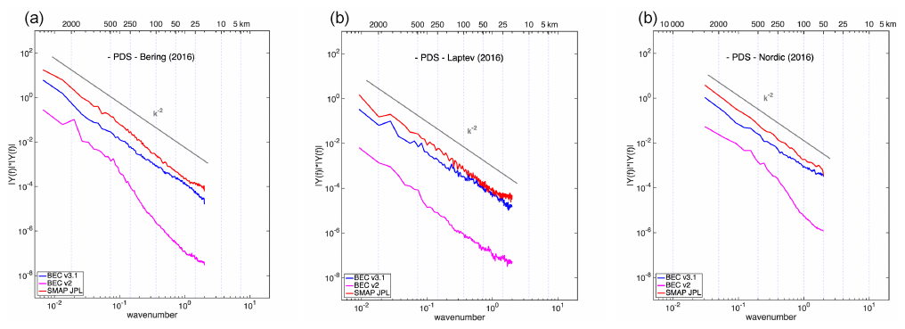
Figure 12Spectral analysis for Arctic+ v3.1, BEC Arctic v2.0, and SMAP products during all of 2016 for different regions: Bering Strait (a), Laptev Sea (b), and Nordic Sea (c).
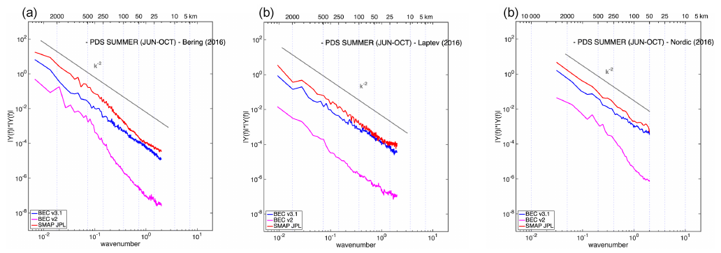
Figure 13Spectral analysis for Arctic+ V3.1, Arctic+v2, and SMAP products for summer (June to October) 2016 for different regions: Bering Strait (a), Laptev Sea (b), and Nordic sea (c).
The product (Martínez et al., 2019) is freely distributed on the BEC (Barcelona Expert Center) web page (http://bec.icm.csic.es/, last access: 25 January 2022) with the DOI number https://doi.org/10.20350/digitalCSIC/12620 (Martínez et al., 2019) and on the Digital CSIC server: https://digital.csic.es/handle/10261/219679 (last access: 25 January 2022). Data can be downloaded from the FTP service: http://bec.icm.csic.es/bec-ftp-service/ (last access: 25 January 2022).
The maps are distributed in the standard grid EASE-Grid 2.0, which has a spatial resolution of 25 km. In addition to the product validated in this work (L3 with temporal resolution of 9 d), L3 products having a temporal resolution of 3 and 18 d and the L2 product are available. These Arctic SSS products cover the period from 2011 to 2019.
This paper presents the methodologies used to produce the new enhanced Arctic+ SMOS SSS v3.1 product developed under the context of the ESA Arctic+Salinity project (AO/1-9158/18/I-BG).
The inversion is performed by using the debiasing non-Bayesian method, as described in Olmedo et al. (2018) and Olmedo et al. (2021), but performing the debiasing at the TB level (refer Martínez et al., 2020, for more details) while in BEC v2.0 the debiasing is performed at the SSS level. Moreover, the temporal bias correction is performed here using GOFS 3.1 (HYCOM + CONDA) data, different than the BEC v2.0 method, which uses the ARGO data.
The SSS maps are produced here by averaging only in time (9 d), but not in space (keeping the same TB resolution). Therefore, there is no loss of effective spatial resolution compared to TB. This finer spatial resolution is one of the main advantages of this product, as shown by the spatial spectral analysis (Sect. 3.4). This new product is preferable to perform studies of the Arctic ocean SSS processes and dynamics.
Arctic+ SSS v3.1 product spans from 2011 to 2019 and consists of daily maps of 9 d averages, in an equal-area grid at 25 km (EASE 2.0 grid). Maps of 3 and 18 d for the same period and grid are also served on the web page, but those products have no specific validation results. Furthermore, the swath SSS product (L2) used to generate the maps is also available on the BEC web page.
The conclusions of the validation procedure are summarized in the following points.
-
Arctic+ v3.1 has, in general, better skill to describe horizontal SSS gradients than BEC v2.0, with better effective spatial resolution. This comes, however, at the price of an increase in bias and a larger uncertainty in some regions.
-
In comparison with Tara datasets, Arctic+ v3.1 shows good agreement with in situ data for some key areas, like the Beaufort Sea, which is one of those areas in the focus of the Arctic scientific community.
-
Comparison with ARGO shows that v3.1 has slightly larger RMSD but presents higher correlation with in situ data. It has been stated that the high spatial resolution of v3.1 produces this larger RMSD when comparing with punctual measurements.
-
The introduction of the correlated triple collocation also helps to properly assess the differences existing between the current (in 2021) derived satellite products. The metrics show that the Arctic+ v3.1 dataset is one of the three products with the lowest errors in general except in Hudson Bay, the east coast of Greenland, and Kara Sea. In particular, the triple collocation shows that SMAP data yield the largest errors.
-
The results of the spatial spectral analysis confirm that Arctic+ v3.1 data have the most consistent spatial representation at smaller scales compared to SMAP and BEC v2.0, allowing a more accurate description of Arctic SSS processes.
JM, CG, AT, EO, and VGG performed the algorithm development. The new algorithms introduced in this version were devised by JM, who also developed the software and generated the products. JM and CG are the main contributors to the writing of this paper. The validation of the products has been carried out by MA, NH, MU, AT, and CGH. All the coauthors have contributed to the writing and revision of the paper.
The contact author has declared that neither they nor their co-authors have any competing interests.
Publisher's note: Copernicus Publications remains neutral with regard to jurisdictional claims in published maps and institutional affiliations.
This work has been carried out as part of the ESA Arctic+Salinity project (AO/1-9158/18/I-BG), which permitted the production of the database, and the Ministry of Economy and Competitiveness, Spain, through the National R&D Plan under L-BAND project ESP2017-89463-C3-1-R. This work represents a contribution to the CSIC Thematic Interdisciplinary Platform PTI Teledetect and PolarCSIC. Argo data were collected and made freely available by the International Argo program and the national programs that contribute to it (https://argo.ucsd.edu, https://www.ocean-ops.org, last access: 25 January 2022). The Argo program is part of the Global Ocean Observing System.
This paper was edited by Giuseppe M. R. Manzella and reviewed by two anonymous referees.
Anterrieu, E., Waldteufel, P., and Lannes, A.: Apodization functions for 2-D hexagonally sampled synthetic aperture imaging radiometers, IEEE T. Geosci. Remote, 40, 2531–2542, https://doi.org/10.1109/TGRS.2002.1176146, 2002. a
Argo: Argo float data and metadata from Global Data Assembly Centre (Argo GDAC), SEANOE, https://doi.org/10.17882/42182, 2018. a
Arias, M., Catany, R., Umbert, M., N., H., Turiel, A., Martínez, J., and Gabarró, C.: Product Validation Report, Arctic+Salinity ITT, Tech. rep., ARGANS, ICM-CSIC, available at: https://arcticsalinity.argans.co.uk/documentation/ (last access: 25 January 2022), 2020. a, b
Blumen, W.: Uniform potential vorticity flow: Part I. Theory of wave interactions and two-dimensional turbulence, J. Atmos. Sci., 35, 774–783, 1978. a, b
Charney, J.: Geostrophic turbulence, J. Atmos. Sci., 28, 1087–1095, 1978. a, b
Cummings, J. A.: Operational multivariate ocean data assimilation, Q. J. Roy. Meteor. Soc., 131, 3583–3604, https://doi.org/10.1256/qj.05.105, 2005. a
Cummings, J. A. and Smedstad, O. M.: Variational Data Assimilation for the Global Ocean, Springer Berlin Heidelberg, Berlin, Heidelberg, 303–343, https://doi.org/10.1007/978-3-642-35088-7_13, 2013. a
Debye, P.: Polar molecules, The Chemical Catalog Company Inc., New York, NY, USA, New York, 1929. a
Dinnat, E. P., Le Vine, D. M., Boutin, J., Meissner, T., and Lagerloef, G.: Remote Sensing of Sea Surface Salinity: Comparison of Satellite and In Situ Observations and Impact of Retrieval Parameters, Remote Sens., 11, 750–785, https://doi.org/10.3390/rs11070750, 2019. a, b
ESA: Earth Observation CFI v3.X branch, ESA, available at: http://eop-cfi.esa.int/index.php/mission-cfi-software/eocfi-software/branch-3-x (last access: 4 October 2019), 2014. a
Font, J., Camps, A., Borges, A., Martin-Neira, M., Boutin, J., Reul, N., Kerr, Y., Hahne, A., and Mechlenburg, S.: SMOS: the challenging sea surface salinity measurement from space, Proc. IEEE, 98, 640–665, 2010. a
Fournier, S., Lee, T., Wang, X., Armitage, T. W. K., Wang, O., Fukumori, I., and Kwok, R.: Sea Surface Salinity as a Proxy for Arctic Ocean Freshwater Changes, J. Geophys. Res.-Oceans, 125, e2020JC016110, https://doi.org/10.1029/2020JC016110, 2020. a
González-Gambau, V., Turiel, A., González-Haro, C., Martínez, J., Olmedo, E., Oliva, R., and Martín-Neira, M.: Triple Collocation Analysis for Two Error-Correlated Datasets: Application to L-Band Brightness Temperatures over Land, Remote Sens., 12, 3381–3422, https://doi.org/10.3390/rs12203381, 2020. a, b
Guimbard, S., Gourrion, J., Portabella, P., Turiel, A., Gabarró, C., and Font, J.: SMOS Semi-Empirical Ocean Forward Model Adjustement, IEEE Trans. Geosci. Remote Sens., 50, 1676–1687, 2012. a
Hoareau, N., Portabella, M., Lin, W., Ballabrera-Poy, J., and Turiel, A.: Error Characterization of Sea Surface Salinity Products Using Triple Collocation Analysis, IEEE T. Geosci. Remote, 56, 5160–5168, https://doi.org/10.1109/TGRS.2018.2810442, 2018. a, b
ICM-CSIC, LOCEAN/SA/CETP, and IFREMER: SMOS SSS L2 Algorithm Theoretical Baseline Document SO-L2-SSS-ACR-007, available at: https://smos.argans.co.uk/docs/deliverables/delivered/ATBD/SO-TN-ARG-GS-0007_L2OS-ATBD_v3.13_160429.pdf (last access: 25 January 2022), 2016. a
Kerr, Y., Waldteufel, P., Wigneron, J.-P., Delwart, S., Cabot, F., Boutin, J., Escorihuela, M.-J., Font, J., Reul, N., Gruhier, C., Juglea, S., Drinkwater, M., Hahne, A., Martin-Neira, M., and Mecklenburg, S.: The SMOS mission: new tool for monitoring key elements of the global water cycle, Proc. IEEE, 98, 666–687, 2010. a
Klein, L. and Swift, C.: An improved model for the dielectric constant of sea water at microwave frequencies, IEEE J. Ocean. Eng., 2, 104–111, https://doi.org/10.1109/JOE.1977.1145319, 1977. a
Lavergne, T., Sørensen, A. M., Kern, S., Tonboe, R., Notz, D., Aaboe, S., Bell, L., Dybkjær, G., Eastwood, S., Gabarro, C., Heygster, G., Killie, M. A., Brandt Kreiner, M., Lavelle, J., Saldo, R., Sandven, S., and Pedersen, L. T.: Version 2 of the EUMETSAT OSI SAF and ESA CCI sea-ice concentration climate data records, The Cryosphere, 13, 49–78, https://doi.org/10.5194/tc-13-49-2019, 2019. a, b
Manabe, S., S. R.: Simulation of abrupt climate change induced by freshwater input to the North Atlantic Ocean., Nature, 378, 165–167, 1995. a
Martínez, J., Gabarró, C., and Turiel, A.: Arctic Sea Surface Salinity L2 orbits and L3 maps (V.3.1), DIGITAL.CSIC [data set], https://doi.org/10.20350/digitalCSIC/12620, 2019. a, b, c, d
Martínez, J., Gabarró, C., and Turiel, A.: Algorithm Theoretical Basis Document, Arctic+Salinity ITT, Tech. rep., BEC, Institut de Ciencies del Mar-CSIC, https://doi.org/10.13140/RG.2.2.12195.58401, 2020. a, b, c, d
Matos, P., Gutiérrez, A., and Moreira, F.: SMOS L1 Processor Discrete Global Grids Document SMOS-DMS-TN-5200, DEIMOS, version 1.4, 2004. a
Mecklenburg, S., Wright, N., Bouzina, C., and Delwart, S.: Getting down to business – SMOS operations and products, ESA Bulletin, 137, 25–30, 2009. a
Meissner, T. and Wentz, F. J.: The complex dielectric constant of pure and sea water from microwave satellite observations, IEEE T. Geosci. Remote, 42, 1836–1849, https://doi.org/10.1109/TGRS.2004.831888, 2004. a, b
Meissner, T. and Wentz, F. J.: The Emissivity of the Ocean Surface Between 6 and 90 GHz Over a Large Range of Wind Speeds and Earth Incidence Angles, IEEE T. Geosci. Remote, 50, 3004–3026, https://doi.org/10.1109/TGRS.2011.2179662, 2012. a, b
Oliva, R., Daganzo, E., Richaume, P., Kerr, Y., Cabot, F., Soldo, Y., Anterrieu, E., Reul, N., Gutierrez, A., Barbosa, J., and Lopes, G.: Status of Radio Frequency Interference (RFI) in the 1400–1427 MHz passive band based on six years of SMOS mission, Remote Sens. Environ., 180, 64–75, https://doi.org/10.1016/j.rse.2016.01.013, 2016. a
Olmedo, E., Martínez, J., Umbert, M., Hoareau, N., Portabella, M., Ballabrera-Poy, J., and Turiel, A.: Improving time and space resolution of SMOS salinity maps using multifractal fusion, Remote Sens. Environ., 180, 246–263, https://doi.org/10.1016/j.rse.2016.02.038, 2016. a
Olmedo, E., Martínez, J., Turiel, A., Ballabrera-Poy, J., and Portabella, M.: Debiased non-Bayesian retrieval: A novel approach to SMOS Sea Surface Salinity, Remote Sens. Environ., 193, 103–126, https://doi.org/10.1016/j.rse.2017.02.023, 2017. a
Olmedo, E., Gabarró, C., González-Gambau, V., Martínez, J., Ballabrera-Poy, J., Turiel, A., Portabella, M., Fournier, S., and Lee, T.: Seven Years of SMOS Sea Surface Salinity at High Latitudes: Variability in Arctic and Sub-Arctic Regions, Remote Sens., 10, 1772–1796, https://doi.org/10.3390/rs10111772, 2018. a, b
Olmedo, E., González-Haro, C., Hoareau, N., Umbert, M., González-Gambau, V., Martínez, J., Gabarró, C., and Turiel, A.: Nine years of SMOS sea surface salinity global maps at the Barcelona Expert Center, Earth Syst. Sci. Data, 13, 857–888, https://doi.org/10.5194/essd-13-857-2021, 2021. a, b, c
Press, W. P., Teukolsky, S., Vetterling, W., and Flannery, B.: Numerical recipes in C (2nd ed.): the art of scientific computing, December 1992, Cambridge University Press, 40 W. 20 St., New York, NY, United States 994 pp., ISBN 978-0-521-43108-8, 1992. a
Reul, N., Tenerelli, J., Chapron, B., and Waldteufel, P.: Modeling Sun glitter at L-band for sea surface salinity remote sensing with SMOS, IEEE T. Geosci. Remote., 45, 2073–2087, 2007. a
Reul, N., Grodsky, S., Arias, M., Boutin, J., Catany, R., Chapron, B., D'Amico, F., Dinnat, E., Donlon, C., Fore, A., Fournier, S., Guimbard, S., Hasson, A., Kolodziejczyk, N., Lagerloef, G., Lee, T., Le Vine, D., Lindstromn, E., Maes, C., Mecklenburg, S., Meissner, T., Olmedo, E., Sabia, R., Tenerelli, J., Thouvenin-Masson, C., Turiel, A., Vergely, J., Vinogradova, N., Wentz, F., and Yueh, S.: Sea surface salinity estimates from spaceborne L-band radiometers: An overview of the first decade of observation (2010–2019), Remote Sens. Environ., 242, 111769, https://doi.org/10.1016/j.rse.2020.111769, 2020. a
Reverdin, G., Le Goff, H., Tara Oceans Consortium, C., and Tara Oceans Expedition, P.: Properties of seawater from a Sea-Bird TSG temperature and conductivity sensor mounted on the continuous surface water sampling system during campaign TARA_20090913Z of the Tara Oceans expedition 2009–2013, PANGAEA, https://doi.org/10.1594/PANGAEA.836924, 2014. a
Sabater, J. and De Rosnay, P.: Milestone 2 Tech Note – Parts 1/2/3: Operational Pre-processing chain, Collocation software development and Offline monitoring suite, Tech. rep., ECMWF, 2010. a
Snyder, J.: Map Projections, A Working Manual, U.S. Geological Survey Professional Paper 1395, U.S. Government Printing Office, Washington D.C., 1987. a
Stoffelen: Toward the true near-surface wind speed: Error modeling and calibration using triple collocation, J. Geophys. Res.-Oceans, 103, 7755–7766, https://doi.org/10.1029/97JC03180, 1998. a, b
Tang, W., Fore, A., Yueh, S., Lee, T., Hayashi, A., Sanchez-Franks, A., Martinez, J., King, B., and Baranowski, D.: Validating SMAP SSS with in situ measurements, Remote Sens. Environ., 200, 326–340, https://doi.org/10.1016/j.rse.2017.08.021, 2017. a, b
Tang, W., Yueh, S. H., Fore, A. G., and Hayashi, A. K.: An Empirical Sea Ice Correction Algorithm for SMAP SSS Retrieval in the Arctic Ocean, in: IGARSS 2020–2020 IEEE International Geoscience and Remote Sensing Symposium, 5639–5642, https://doi.org/10.1109/IGARSS39084.2020.9323740, 2020. a
Tenerelli, J. E., Reul, N., Mouche, A. A., and Chapron, B.: Earth Viewing L Band Radiometer Sensing of Sea Surface Scattered Celestial Sky Radiation-Part I: General Characteristics, Geoscience and Remote Sensing, IEEE Transactions on, 46, 659–674, 2008. a
Tukey, J.: Exploratory data analysis, Addison-Wesley, Lebanon, Indiana, USA Pearson, ISBN-13 978-0201076165, ISBN-10 0201076160, 1977. a, b
West, S. G., Finch, J. F., and Curran, P. J.: Structural equation models with nonnormal variables: Problems and remedies, in: Hoyle, R. H., Structural equation modeling: Concepts, issues, and applications, Sage Publications, Inc., 56–75, 1995. a
Yueh, S., West, R., Wilson, W., Li, F., Nghiem, S., and Rahmat-Samii, Y.: Error Sources and Feasibility for Microwave Remote Sensing of Ocean Surface Salinity, IEEE T. Geosci. Remote, 39, 1049–1059, 2001. a
Zhou, Y., Lang, R. H., Dinnat, E. P., and Vine, D. M. L.: L-Band Model Function of the Dielectric Constant of Seawater, IEEE T. Geosci. Remote, 55, 6964–6974, https://doi.org/10.1109/TGRS.2017.2737419, 2017. a
Zine, S., Boutin, J., Font, J., Reul, N., Waldteufel, P., Gabarro, C., Tenerelli, J., Petitcolin, F., Vergely, J., Talone, M., and Delwart, S.: Overview of the SMOS Sea Surface Salinity Prototype Processor, IEEE T. Geosci. Remote, 46, 621–645, https://doi.org/10.1109/TGRS.2008.915543, 2008. a, b
Zweng, M. M., Reagan, J. R., Antonov, J. I., Locarnini, R. A., Mishonov, A. V., Boyer, T. P., Garcia, H. E., Baranova, O. K., Johnson, D. R., Seidov, D., and Biddle, M. M.: World Ocean Atlas 2013, volume 2, Salinity, Levitus, A. Mishonov Technical Ed., NOAA Atlas NESDIS 74, 39 pp., 2013. a
Zweng, M. M., Reagan, J. R., Seidov, D., Boyer, T. P., Locarnini, R., Garcia, H. E., Mishonov, A., Baranova, O. K., Weathers, K., PAver, C., and Smolyar, I.: World Ocean Atlas 2018, volume 2, Salinity, A. Mishonov Technical Ed., NOAA Atlas NESDIS 82, 50 pp., 2018. a, b, c, d
The requested paper has a corresponding corrigendum published. Please read the corrigendum first before downloading the article.
- Article
(2049 KB) - Full-text XML