the Creative Commons Attribution 4.0 License.
the Creative Commons Attribution 4.0 License.
 | 27 Jan 2022
A national extent map of cropland and grassland for Switzerland based on Sentinel-2 data
Nica Huber
Dominique Weber
Christian Ginzler
Bronwyn Price
Agricultural landscapes support multiple functions and are of great importance for biodiversity. Heterogeneous agricultural mosaics of cropland and grassland commonly result from variable land use practices and ecosystem service demands. Switzerland's agricultural land use is considerably spatially heterogeneous due to strong variability in conditions, especially topography and climate, thus presenting challenges to automated agricultural mapping. Nationwide knowledge of the location of cropland and grassland is necessary for effective conservation and land use planning. We mapped the distribution of cropland and permanent grassland across Switzerland. We used several indices largely derived from Sentinel-2 satellite imagery captured over multiple growing seasons and parcel-based training data derived from landholder reporting. The mapping was conducted within Google Earth Engine using a random forest classifier. The resulting map has high accuracy in lowlands as well as in mountainous areas. The map will act as a base agricultural land cover dataset for researchers and practitioners working in agricultural areas of Switzerland and interested in land cover and landscape structure. The map as well as the training data and calculation algorithms (using Google Earth Engine) are freely available for download on the EnviDat platform https://doi.org/10.16904/envidat.205 (Pazúr et al., 2021).
- Article
(12654 KB) - Full-text XML
-
Supplement
(63 KB) - BibTeX
- EndNote


Cropland and grassland cover 34 % of the earth's terrestrial surface and represent the second most widespread land cover (LC) class, after forests (36 %) (Buchhorn et al., 2020). Cropland and grassland provide multiple services for humans and nature, for example, food and fodder provisioning, habitat for various species, or cultural heritage (Bengtsson et al., 2019). The provisioning of these services varies substantially across the globe and is influenced by climate, cultural factors, and the spatial and temporal configuration of landscape types. Areas with multiple use demands require a high degree of landscape multifunctionality. In multifunctional landscapes, the spatial allocation of cropland and grassland is strongly influenced by management policies supporting production and protection services in different forms and structures (e.g. grassland subsidies for management practices, usually related to mowing, grazing and fertilizing regimes). Sustainable management strategies may help to maintain vulnerable ecosystems in agricultural areas, increase biodiversity or minimize the risks associated with inappropriate management (e.g. soil erosion or degradation of grassland ecosystems) (Wezel et al., 2014). Therefore, knowledge of the spatial mosaic of cropland and grassland is extremely important. Such maps also determine the design of ecological networks and evaluation of current and future management strategies.
Accurate maps of agricultural areas at high spatial resolution and available at national scales have previously been very rare. Only recently has it been possible for demands for such maps of agricultural areas to be met through the undertaking of several national or international projects, thanks to the increasing availability of open-access remote sensing data. For example, mapping of grasslands and their management has been conducted at the national extent for Germany (Griffiths et al., 2019). A grassland map is also part of the Copernicus Land Monitoring Service High Resolution Layer group for Europe produced by European Environmental Agency (Copernicus Land Monitoring Service, 2020). In comparison to European scale products, nationwide products can benefit from better parametrization of classification model(s) to account for the sub-continental variation within agricultural areas (e.g. in field size and mosaics) which occurs within Europe due to different management practices or climatic conditions.
We mapped cropland and permanent grassland across the whole of Switzerland. Switzerland covers 41 285 km2 and is well suited to the development and testing of methods for mapping agricultural land cover due to the availability of extensive ground-truth data. Despite being a small country, Switzerland is very heterogeneous with respect to climate and terrain conditions which have a strong influence over the ecosystems services provided by agricultural land (Fig. 1), as well as in socio-political terms with variation across the 26 cantons. Switzerland is divided into six biogeographical regions (Fig. 1) defined following statistical analysis of the distribution of flora and fauna species and adapted to boundaries of communes (Gonseth et al., 2001; Wohlgemuth, 1996). These regions differ significantly in their climate and topography. The demand for ecosystem services provided by agricultural areas is relatively high compared to other European countries since the import of agricultural goods is relatively limited (compared to EU member states) and protection measures are applied across agricultural areas. Protection measures include designation of strict protection areas where fertilization and irrigation are banned, as well as measures that control the timing and number of management activities such as mowing, grazing and fertilization of grasslands (Boch et al., 2019). In addition, direct payment schemes are also used to manage arable land requiring implementation of crop rotation and managed fertilizer regimes, restrictions on pesticides use, and compulsory implementation of buffer zones and ecological compensation areas (FOAG, 2015). As a result, areas which are topographically suitable for arable agriculture (which are relatively limited) are likely subject to intensive farming.

Figure 1Biogeographic regions and shaded relief of Switzerland.
We used Sentinel-2 imagery from the growing seasons of 2017–2019 to map cropland, permanent grassland and shrubland at 10 m resolution. Although we tested a model using imagery from a single year (2019), we found that this approach resulted in lower accuracies than multi-year data. Since our aim was to differentiate permanent grassland from cropland, temporary/annual grassland was considered part of the crop rotation, and as such multi-year imagery was more fit to our purpose. We trained and parameterized a random forest classifier within the Google Earth Engine (GEE), using multiple Sentinel-2 indices on selected agricultural parcels from all over Switzerland, for which information was available on the crop and grassland types cultivated in a specific year. Using a cross-validation (split-sample) approach we found that the resulting map reached an overall accuracy of 84 %–95 % in the Jura and Plateau region and 90 %–95 % in Alps. The misclassified pixels were mostly grasslands falsely assigned to cropland areas and mostly related to annual grasslands, which were considered to be cropland within the training data. The resulting map of cropland (including annual grassland) and permanent grassland provides a spatially explicit, area-wide alternative to the only existing national dataset, the Swiss Land Use Statistics, which is a point-based statistical dataset on a 100 m grid (Bundesamt für Statistik, 2020). The application combines two models, one stratified for the Alps and one for the areas outside of the Alps, and as such the trained model is also applicable within different biomes. There is potential for the trained model and classification algorithm to be transferable to map cropland and grassland in different growing seasons or in different countries assuming similar agricultural management practices and climatic conditions.
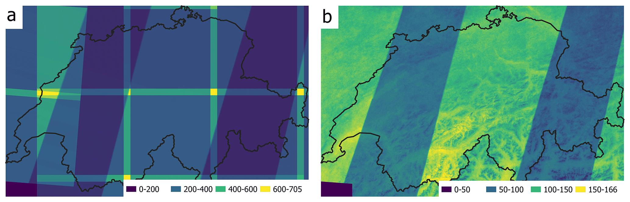
Figure 2The number of available Sentinel-2 scenes (a) prior to the cloud masking including tile edge effect and (b) after applying the cloud mask and masking of the scene edges.
2.1 Satellite imagery
To identify cropland, grassland and shrubland, we used spectral information
retrieved from all Sentinel-2 pixels available for Switzerland between
April–November of 2017–2019 with initial cloud coverage lower than 80 %
(as reported in the Sentinel-2 metadata). We used the Sentinel-2 imagery
preprocessed to surface reflectance (Level 2A) within GEE (GEE repository
ee.ImageCollection(“COPERNICUS/S2_SR”)) and applied a cloud
masking procedure (GEE repository
ee.ImageCollection(“COPERNICUS/S2_CLOUD_
PROBABILITY”). This procedure uses deep learning semantic segmentation
(Garcia-Garcia et al., 2017) to set the cloud
occurrence probabilities within Sentinel-2 scenes (Zupanc, 2017)
and has been documented to outperform other cloud masking procedures.
Additional scripts were used to mask shadows and snow coverage (see the
linked GEE codes for more information). After preprocessing, the number of
images available within the time period varied substantially over
Switzerland due to cloudiness, especially in the Alps, and the acquisition
pathways of the Sentinel-2 satellite sensors (Fig. 2).
2.2 Training data
To identify the spectral parameters of cropland and grassland, we used parcel-level training data indicating the occurrence of different crop types and permanent grassland derived by cantonal (state) authorities based on the reporting of farmers in the years 2017–2019. We have considered parcels with reported crop usage (e.g. wheat, spelt, corn, potatoes, sugar beets) within a reported year to be cropland. Due to the practise of crop rotation which is frequently applied on Swiss agricultural parcels, as well as different crop type within an individual field, it is likely that the spectral characteristics of a given single parcel changed within the 3-year study period. However, the training data for each parcel are for one time point only within the study period, and therefore such temporal variations were not considered within the training data. Cropland is considered to be an area covered by crops within a given year for particular training data, while grasslands are considered to be areas explicitly reported as permanent grasslands. Permanent grasslands are likely to have similar phenological trajectories over the multiple growing seasons considered within the study period. Parcels classified as annual grasslands within the reported statistics were considered to be cropland because we considered annual grassland to be a part of the crop rotation management.
The parcel-level training polygons were selected manually from different areas across Switzerland. The overall requirement for selection of a polygon was its visual homogeneity (e.g. no trees within the cropland or grassland fields). We also considered the variability of croplands and grasslands by including parcels that reported different land use within those two classes (e.g. different cropland types). To avoid selecting pixels of mixed land use, which are likely to occur in heterogeneous landscapes, especially at parcel edges, we shrunk the training polygons by a 10 m “inside” buffer distance (buffer size defined according to the resolution of Sentinel-2 bands). In total, 1378 polygons covered by more than 400 000 10 m pixels were selected to train the classification model.
In addition to the cropland and grassland data, we provided the random forest (RF) model with training data on shrubland, forest, wetland and water surfaces. These training data allowed us to better define the ranges of reflectance of different LC in the training data. In the accuracy assessment we only include the shrubland as it is a widespread LC class in Swiss mountainous areas and, due to its vegetation cover with minimal seasonal variation in reflectance, is likely to be considered grassland by our predictive models. Other LC classes were further masked out using different maps and were not an object of accuracy testing. Training data on different LC classes were generated from 70, 25 and 13 polygons with an average area of 11, 30 and 1177 ha for shrubland, wetland and water surfaces, respectively. These polygons were digitized manually from the Sentinel-2 imagery guided by the Swiss Land Use Statistics.
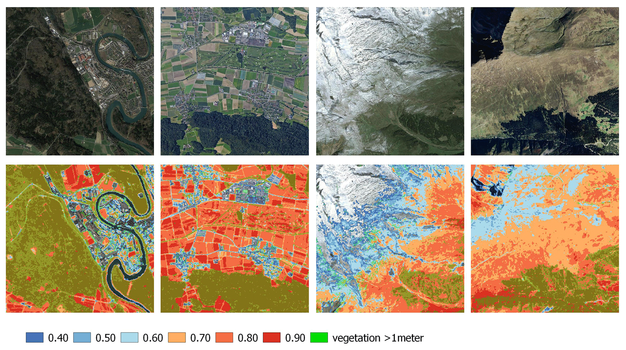
Figure 3Illustration of the performance of different layers considered to mask out sealed areas, water surfaces and rocks from the resulting map. The values represent different NDVI value thresholds observed at the 95th percentile. Green outlines show the areas of vegetation taller than 1 m (source of the aerial imagery: © Google Maps).
2.3 Classification indices
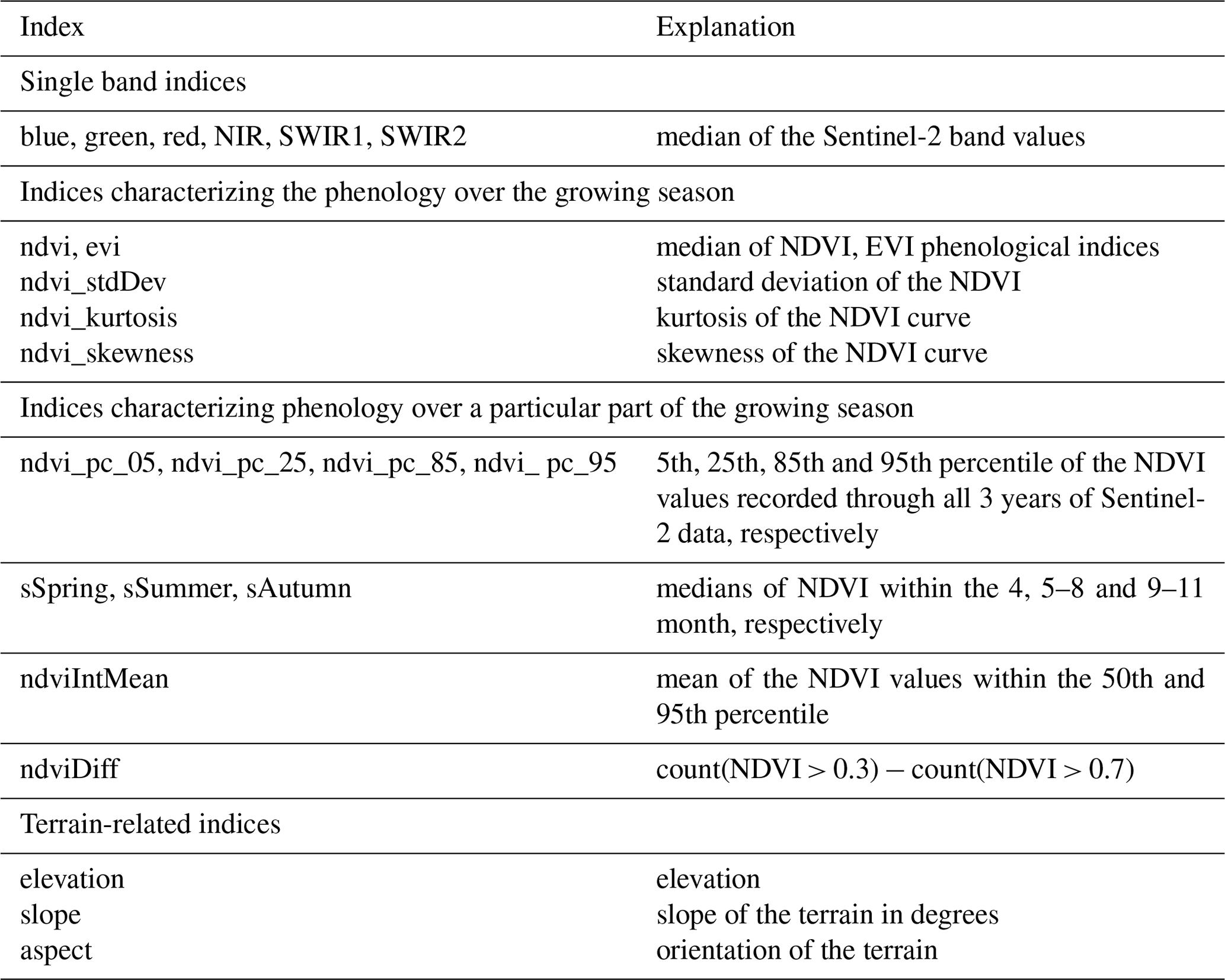
We extracted multiple indices for every Sentinel-2 pixel overlapping the training polygons. The indices used were chosen based on previous mapping of Swiss agricultural areas (Kolecka et al., 2018; Pazúr et al., 2021) and followed general assumptions about the differences between the phenology of cropland and grassland over a year (e.g. low growth on cropland in autumn) and low variability of permanent grassland over time. The selected indices characterize phenology either over the whole growing season or over a particular part of the growing season, or they relate to summary statistics of the spectral bands of Sentinel-2 (Table 1). Similar indices have been found useful for land cover classification over large areas (Pflugmacher et al., 2019) and mapping phenological responses in grassland areas or cropland types (Ghazaryan et al., 2018; Gómez Giménez et al., 2017). Furthermore, we included variables characterizing the terrain properties of each pixel, such as elevation, slope and terrain orientation retrieved from the 30 m Shuttle Radar Topography Mission data (GEE repository ee.ImageCollection (“USGS/SRTMGL1_003”) (Farr et al., 2007).
Table 1Indices used in the classification model as calculated from the growing seasons of 3 years of Sentinel-2 satellite data.
2.4 Classification
To account for different environmental conditions (i.e. climate and terrain) within Switzerland, the classification models were calculated separately for two strata defined by biogeographic regions. The biogeographical regions of the Jura Mountains and the Swiss Plateau together form one stratum (regions 3 and 4 on Fig. 1), while the Alpine regions form a second stratum (regions 1, 2, 5 and 6 on Fig. 1). While we tested several approaches to defining the strata, including a single national model and different combinations of the biogeographical regions, we found that the two strata chosen gave the best results and most straightforward approach to taking into account the climatic and topographical differences between the more lowland areas and the mountainous areas. In particular the whole of Switzerland approach resulted in biases for crop detection towards the Plateau and higher inaccuracies in mountainous areas, particularly in mixed shrubland grassland areas.
We used the random forest (RF) classifier implemented within the GEE platform (library ee.Classifier.smileRandomForest) for the classification of cropland, grassland and shrubland. The default parameters of the GEE algorithm were used except for the number of trees (300 trees were used) and the number of variables per split (10 variables per split were used). These variables were set according to the accuracy cross-validation checks of different combinations of their values (Kuhn, 2008). We also produced a separate layer of non-vegetated areas, i.e. sealed surfaces, rocks and water bodies for masking purposes. Assuming that those surfaces have little or no phenological response, we classified these areas using the 95th percentile of the distribution of all normalized difference vegetation index (NDVI) values recorded over the mapping period. Using two different thresholds, we found the non-vegetated areas under 2000 m a.s.l. on those pixels where the 95th percentile of recorded NDVI value was lower than 0.7. In areas above 2000 m a.s.l., the non-vegetated areas occurred where the 95th percentile of recorded NDVI value was lower than 0.6 (Fig. 3).
2.5 Postprocessing
To increase the accuracy of the final map we masked out woody vegetation (forest, tree lines and single trees) from the model output with the vegetation height model (VHM) of Switzerland (Ginzler and Hobi, 2015). Within areas classified as cropland, woody vegetation was masked out using a vegetation height threshold of 3 m. This was done to prevent the exclusion of crops that potentially reach 3 m in height, especially towards the end of the growing season (the period when the imagery on which the VHM is based was captured). Within grasslands, a lower threshold of 1 m was applied in order to mask out vineyards, shrubs and hedgerows. In addition, we converted all cropland areas smaller than 2000 m2 to grassland as we considered this a minimum size for cropland parcels. This allowed us to eliminate the effects of misclassification of LC on mixed pixel areas, such as in settlement hinterland or at high elevations, where small patches of grassland may appear within areas of low vegetation cover, e.g. in the transition zone between grassland and rocks. As it is likely that all the areas of forest were masked out using the VHM, we converted all the unmasked pixels of forest to shrubland as we found large uncertainties of distinguishing between those two classes within our model.
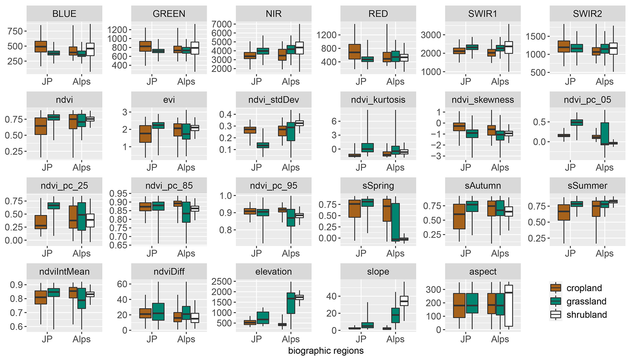
Figure 4Value ranges of indices within the training samples used to model the allocation of cropland and grassland stratified by biogeographic regions of (JP) Jura and Plateau and (Alps) Alps. For indices' abbreviation details please refer to Table 1.
2.6 Accuracy assessment
Map accuracy was assessed against three separate testing datasets: the “parcel-level+” testing dataset, derived from parcel-level data and digitized polygons of other LC classes derived in a similar manner to that described in Sect. 2.2 (Training data section), and two independent datasets, the ALL-EMA (Agricultural Species and Habitats' Monitoring Programme) (Riedel et al., 2018) testing dataset and the Swiss Land Use Statistics testing dataset, described further below. Since these datasets were produced independently and for differing purposes, each dataset has differences in extent, nomenclature and ground-truth information.
2.6.1 Parcel-level testing dataset
To assess map accuracy using the parcel-level data, we trained separate random forest models (one for Jura and Plateau and one for Alps) using the R software random forest package (Liaw and Wiener, 2002) and training data and settings similar to the classification in GEE. In this case, the manually generated training dataset and digitized shrubland areas used to train the classification in GEE were split into training and testing datasets (80 % of the polygons were used to train and 20 % to test the model). Using a separate model allowed us to avoid redundancies associated with using the same data for training and testing (i.e. avoid to use the map that was produced from the full training dataset). To limit spatial clustering, we further limited the selected samples in each biogeographical strata by maintaining a minimum distance of 30 m between selected samples.
The accuracy of the outputs was measured using the overall accuracy and the related sensitivity and specificity rates. In our case, sensitivity is defined as the proportion of correctly classified presences of grassland for the Jura and Plateau region or of each class for the Alps region. In contrast, specificity is defined as the proportion of correctly classified absences of a particular class. Class level accuracies were calculated since they do not inherit the bias that may be present in an overall accuracy measure (Foody, 2020).
2.6.2 All-EMA testing dataset
ALL-EMA, the Agricultural Species and Habitats' Monitoring Programme (Riedel et al., 2018, 2019), is a Swiss monitoring programme designed to monitor biodiversity on agricultural land. Among other measurements, it records habitat and land use type on 170 1 km2 area squares through field visits, with an average of 19 10 m2 plots monitored on each of these squares (Riedel et al., 2018). Only data points from ALL-EMA – locations of cropland, grassland and shrubland habitat – which overlap the output map were included in the comparison.
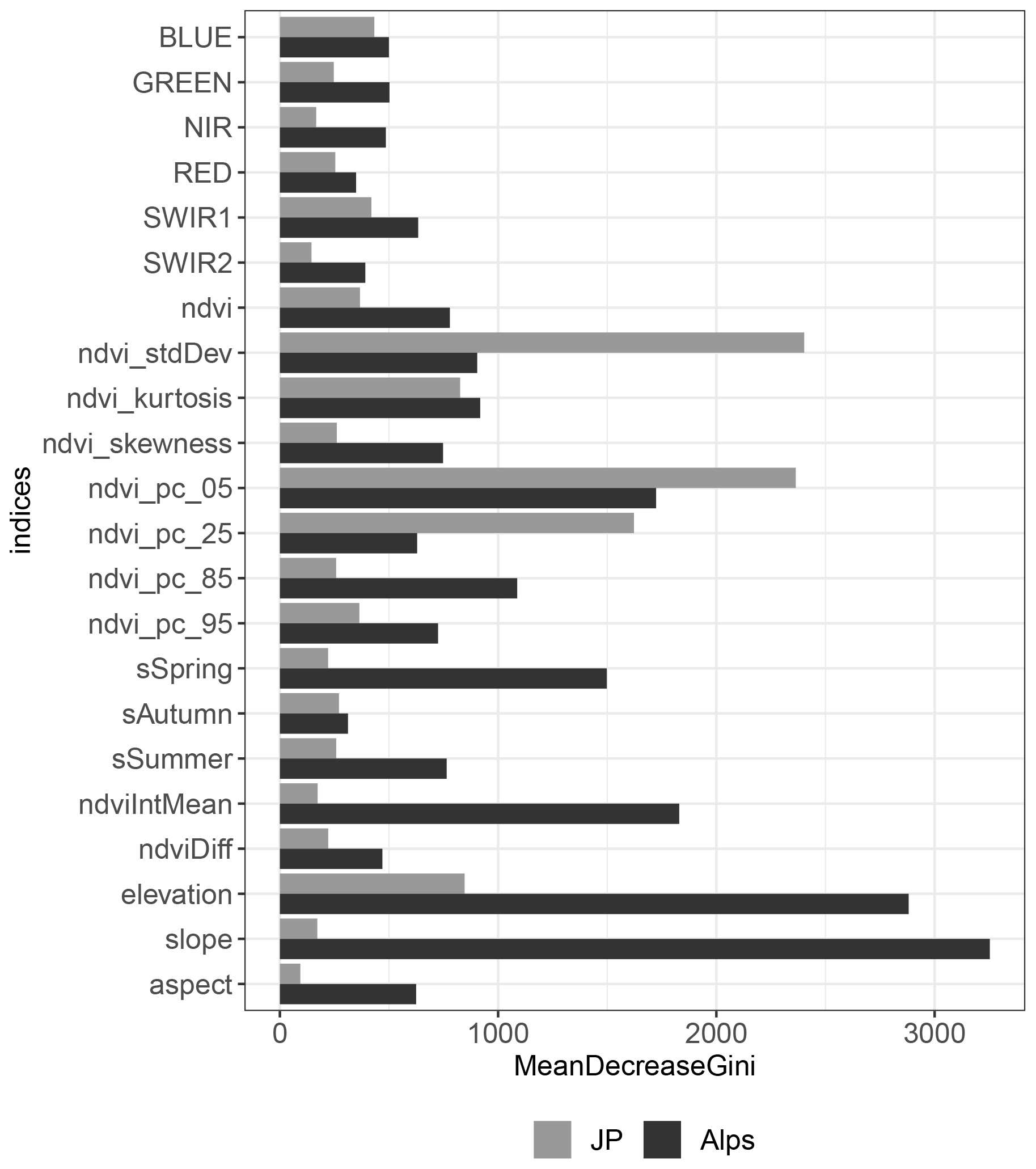
Figure 5Importance of different indices in the classification model within the Jura and Plateau stratum (JP) and the Alps (Alps) quantified using the mean value of the Gini-impurity loss function coefficient. More important indices in the model achieved higher values of the coefficient.
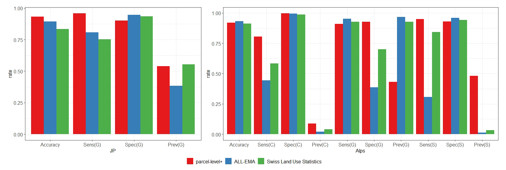
Figure 6Accuracy rates of the classification of (C) cropland and (G) grassland on the Jura and Plateau region (JP) and (C) cropland, (G) grassland and (G) shrubland on the Alps (Alps). Shrubland was not considered in the Jura and Plateau region; the sensitivity values (Sens(G)) reflect the correctly classified presence of grassland and the specificity (Spec(G)) the absence of grassland, i.e. presence of cropland. The proportion of presence of grassland within the samples is indicated by prevalence (Prev).
2.6.3 Swiss Land Use Statistics
The Swiss Land Use Statistics dataset is a nationwide point sample of land use and cover information on a 100 m grid across Switzerland (Riedel et al., 2018, 2019). The standard nomenclature of the Swiss Land Use Statistics dataset comprises 72 unique categories combining land use and cover classes, and each point of the dataset is interpreted visually from aerial photography and additional datasets. This approach ensures relatively accurate and robust land use and cover information for a given point and date (generally defined by the capture date of the aerial imagery). The Swiss Land Use Statistics dataset was used to assess the spatial pattern of accuracy of our cropland and grassland map within blocks of 1 km2 in size (100 interpretation points per block). The 1 km2 blocks allowed us to identify the areas of agreement and mismatch between both datasets. The Swiss Land Use Statistics dataset is updated every 12 years, the current cycle 2013–2018 is still being processed and not yet available for the full extent of Switzerland. Therefore, for the nationwide assessment of cropland and grassland areas, we complemented the 2013/2018 dataset with data from the 2004/2009 survey areas where data from the current survey were not yet available (circa 17 %). The following classes were considered to be grassland: natural grassland, farm pasture, mountain meadow, alpine, Jura, and sheep pasture and unproductive grassland if covered by grass. The Swiss Land Use Statistics cropland class was used for crops.
The output map (stored in the GeoTIFF 8-bit unsigned integer file format) identifies areas of cropland (value 1), permanent grassland (value 2) and shrubland (value 3) at 10 m resolution over the entire area of Switzerland. Areas of shrubland, tall vegetation (forest and trees), sealed surfaces, water and rocks are masked out. Furthermore, patches of cropland smaller than 2000 m2 have been converted to grassland because they are assumed to be a result of misclassification. To apply these type of conversions that rely on the definition of raster patch sizes, we recommend the r.li toolset implemented in GRASS GIS and QGIS software (Neteler et al., 2012; QGIS, 2020) or the RegionGroup tool in ArcGIS software (ESRI, 2016).
Since the unmasked map of cropland, grassland and shrubland might be helpful for certain ecological applications, we also published a version of the map with unmasked shrubland as well as the masks of non-vegetated areas (see the classification section of this paper, Sect. 2.4). The resulting maps and codes are available on the EnviDat portal (Pazúr et al., 2021) under the following link: https://doi.org/10.16904/envidat.205.
The GEE code also links the datasets used to train and mask the output map.
Table 2Error matrix based on the ratios of true–false observations.

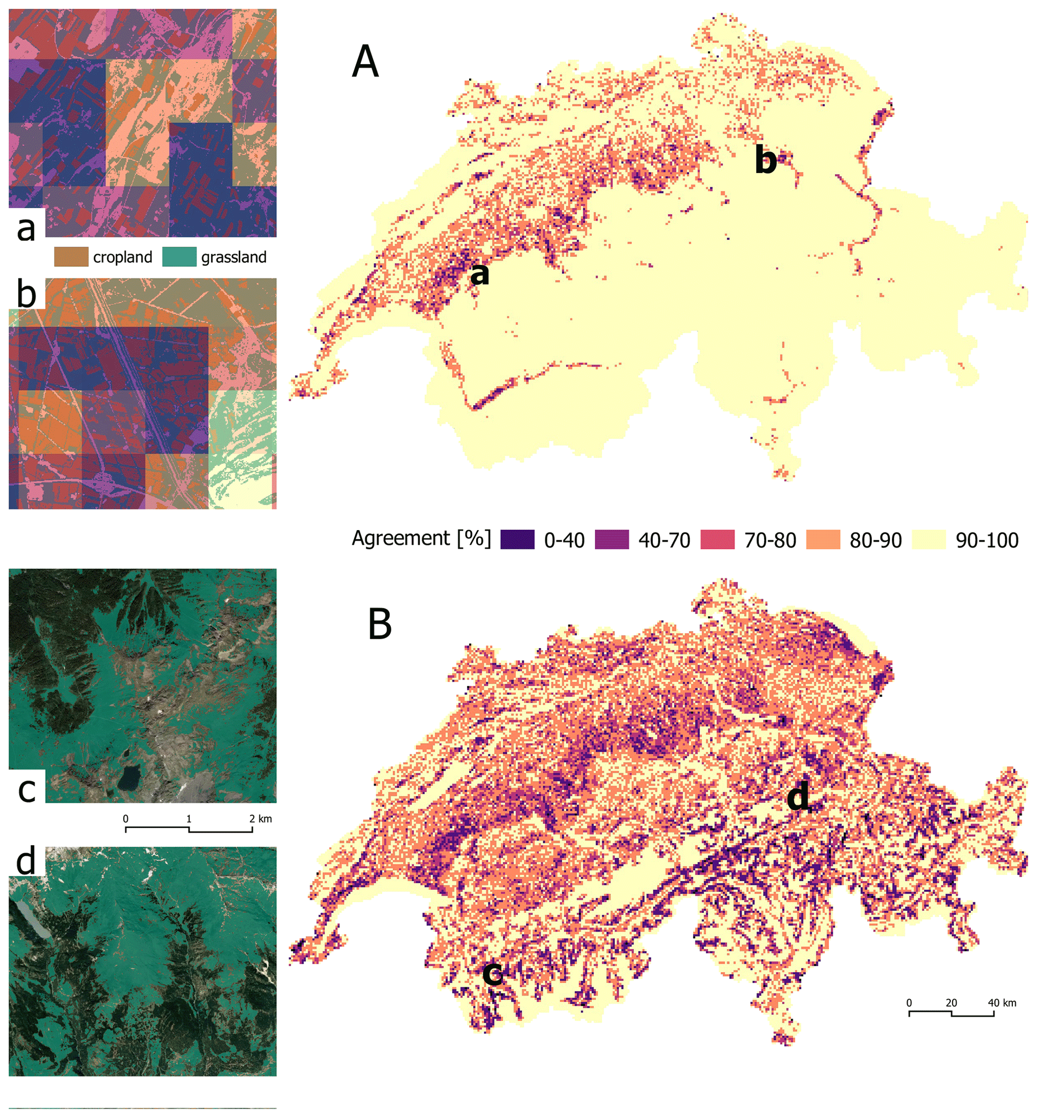
Figure 7Agreement [%] between (A) the cropland map and the reference classification (Swiss Land Use Statistics) and between (B) the grassland map and the reference classification (Swiss Land Use Statistics) per 1 km2 block (100 interpretation points per block). The rectangular close-ups show the distribution of cropland and grassland (a, b) and grassland (c, d) in selected areas with less precise classification outcomes.
4.1 Classification indices
The distribution of the values of the indices derived from Sentinel-2 and the elevation model within the generated samples indicated differences between cropland, grassland and shrubland (Fig. 4). Substantial differences between these LC classes were found for individual spectral bands (NIR, SWIR1, SWIR2), phenological indices (NDVI, EVI and its derivatives) and terrain indices (elevation, slope).

Figure 8Illustration of the agreements between our cropland and grassland mapping output (OUTPUT), various land cover maps with global coverage (PROBA, GLC30, GLC10) and the reference classification (Swiss Land use Statistics, true and false symbols) on selected areas representing lowland (a), mountainous (b) and valley-like (c) terrain conditions. The R statistics defines the producer accuracy.
Using those indices, we found better separability of cropland and grassland for the Jura and Plateau stratum compared to the Alps. Indices that characterize phenology over the growing season generally have higher values on grassland areas than cropland areas except for the standard deviation of NDVI, which is lower on grassland. For the Jura and Plateau stratum the standard deviation of NDVI was found to be one of the most important indices in the classification model (Fig. 5). Grasslands within both strata were also characterized by a negative skewness of the distribution of NDVI values. This relatively high proportion of higher NDVI values reflects the higher greenness of these areas. For shrubland, the values of these indices were within a very narrow span of the value distribution. This suggests the phenological behaviour of shrubland over the growing seasons is less variable than that of cropland or grassland. Good separability between cropland and grassland was also possible through the phenological indices ndvi_pc_05 and ndvi_pc_25, which represent the lower percentiles of the distribution of NDVI recorded through all 3 years of Sentinel-2 data. Especially for the Jura and Plateau stratum, both indices were much higher on grassland than on cropland and highly contribute to the accuracy of the resulting classification model. Within the samples generated for the Jura and Plateau stratum, using the single phenological indices, such as the ndvi_pc_05, may successfully separate cropland and grassland classes. By ensuring the robustness of such metrics for example by including multiple growing seasons, the model generated for the Jura and Plateau stratum may be applicable on flat and less complex terrains elsewhere.
However, we observed a wide range in spring seasonality (sSpring), especially on Alpine grasslands. This observation may be due to the low phenology of the alpine grassland at the beginning of the growing season or snow artefacts, which were missed from the snow mask applied in the classification especially during the snow melting period. Elevation also substantially aided the separation of grasslands from cropland and the classification accuracy, particularly within the Alps stratum. This observation can be considered relevant to mountainous areas, where cropland areas are generally only feasible at comparably lower elevations. Generally, the complex terrain conditions of the Alps, described by the terrain parameters, substantially influenced the separability of the cropland and grassland classes which might limit the transferability of the model outside of the Swiss Alps.
4.2 Accuracy assessment
Comparison between the derived map and the selected test datasets showed high accuracy of the modelling outputs (Fig. 6). The comparison of the output map with the test data derived from the selected parcel-level+ polygons resulted in the highest overall accuracies, 0.93 for the Jura and Plateau region and 0.92 for the Alps region. This accuracy assessment (parcel-level+ data) was also based on samples that were the most equally distributed across the different classes (prevalence ratios). The lowest accuracies were found for the comparison to the ALL-EMA dataset in the Alps regions for the presence of cropland and shrubland, 0.44 and 0.31 (sensitivity ratio), and absence of grasslands, 0.38 (specificity ratio). The prevalence rates, however, demonstrate that these results relate to a limited number of samples. Due to low occurrences and a large number of samples, the prediction of absence of cropland in the Alps was of highest accuracy (0.99, specificity ratio) compared to the ALL-EMA testing data. The accuracy assessment of the shrubland mapping resulted in similarly high accuracy rates for both the parcel-level+ data and the Swiss Land Use Statistics. These similarities are to be expected since the parcel-level+ training data for shrubs were selected from a subset of the Swiss Land Use Statistics. These accuracy assessments only consider areas of overlap between the output map and cropland, grassland, and shrubland as defined by the given testing dataset. Potential bias of the output map outside of this extent, e.g. occurrence of cropland, grasslands and shrublands in areas of woody vegetation, lakes or non-vegetated areas, is not considered.
Furthermore, we assessed the nationwide accuracy of cropland and grassland mapping using all Swiss Land Use Statistics interpretation points (n= 4 128 498). This accuracy assessment resulted in high overall agreement with our classification at 85 % with a user's accuracy of 88 % and 67 % and a producer's accuracy of 72 % and 81 % for cropland and grassland, respectively (Table 2). The lower accuracy may be due to nomenclature differences, which mean that the definitions of cropland and grassland are not fully aligned (e.g. agricultural crop rotation between crop and grassland on the same parcel). Moreover, the Swiss Land Use Statistics are determined from aerial imagery captured over an extensive time span which, depending on location does not match with the period of our mapping data and the spatial resolution of the output map (10 m). By summarizing the spatial distribution pattern of agreement/mismatch within 1 km2 blocks (Fig. 7), a higher degree of mismatch was found in mountainous and sparsely vegetated areas, as well as in wine-making areas. By comparing the cropland and grassland with the Swiss Land Use Statistics, our mapping outcome performed well also in comparison with different land cover mapping products with global coverage (Fig. 8). Specifically, in the case of accuracies of cropland and grassland, the mapping output outperformed the Copernicus Global Land Cover 100 m (PROBA, Buchhorn et al., 2021), Global Land Cover Map in 30 m resolution (GLC30, Zhang et al., 2021) and Global Land Cover Map in 10 m resolution (GLC10, Gong et al., 2019).
The supplement related to this article is available online at: https://doi.org/10.5194/essd-14-295-2022-supplement.
RP designed the study, analysed the data and together with BP prepared the manuscript with contributions from all other co-authors. NH and CG contributed to the methodology design. DW performed the validation of the results.
The contact author has declared that neither they nor their co-authors have any competing interests.
Publisher’s note: Copernicus Publications remains neutral with regard to jurisdictional claims in published maps and institutional affiliations.
This dataset was developed within the project “Erstellung einer Lebensraumkarte Schweiz 2019–2021” conducted at the Swiss Federal Research Institute WSL and funded by the Swiss Federal Office for the Environment.
This research has been supported by the Swiss Federal Office for the Environment.
This paper was edited by Dirk Fleischer and reviewed by two anonymous referees.
Bengtsson, J., Bullock, J. M., Egoh, B., Everson, C., Everson, T., O'Connor, T., O'Farrell, P. J., Smith, H. G., and Lindborg, R.: Grasslands-more important for ecosystem services than you might think, Ecosphere, 10, e02582, https://doi.org/10.1002/ecs2.2582, 2019.
Boch, S., Bedolla, A., Ecker, K. T., Ginzler, C., Graf, U., Küchler, H., Küchler, M., Nobis, M. P., Holderegger, R., and Bergamini, A.: Threatened and specialist species suffer from increased wood cover and productivity in Swiss steppes, Flora, 258, 151444, https://doi.org/10.1016/j.flora.2019.151444, 2019.
Buchhorn, M., Lesiv, M., Tsendbazar, N. E., Herold, M., Bertels, L., and Smets, B.: Copernicus global land cover layers-collection 2, Remote Sens., 12, 1–14, https://doi.org/10.3390/rs12061044, 2020.
Buchhorn, M., Smets, B., Bertels, L., Roo, B. De, Lesiv, M., Tsendbazar, N.-E., Li, L., and Tarko, A.: Copernicus Global Land Service: Land Cover 100 m: version 3 Globe 2015–2019: Product User Manual, Zenodo [data set], https://doi.org/10.5281/zenodo.4723921, 2021.
Bundesamt für Statistik: Arealstatistik Schweiz, Neuchâtel, [data set], available at: https://www.bfs.admin.ch/bfs/de/home/statistiken/raum-umwelt/erhebungen/area.html (last access: 20 June 2021), 2020.
Copernicus Land Monitoring Service: Grassland 2018 and Grassland change 2015–2018, [data set] available at: https://land.copernicus.eu/pan-european/ (last access: 20 June 2021), 2020.
ESRI: ArcGIS Desktop: Release 10.3, available at: https://desktop.arcgis.com/ (last access: 20 June 2021), 2016.
Farr, T. G., Rosen, P. A., Caro, E., Crippen, R., Duren, R., Hensley, S., Kobrick, M., Paller, M., Rodriguez, E., Roth, L., Seal, D., Shaffer, S., Shimada, J., Umland, J., Werner, M., Oskin, M., Burbank, D., and Alsdorf, D.: The Shuttle Radar Topography Mission, Rev. Geophys., 45, RG2004, https://doi.org/10.1029/2005RG000183, 2007.
FOAG: Biodiversity for food and agriculture in Switzerland, Abridged version and main findings of Switzerland’s Country Report on the State of Biodiversity for Food and Agriculture, Bern, 78 pp., available at: https://www.blw.admin.ch/ (last access: 20 June 2021), 2015.
Foody, G. M.: Explaining the unsuitability of the kappa coefficient in the assessment and comparison of the accuracy of thematic maps obtained by image classification, Remote Sens. Environ., 239, 111630, https://doi.org/10.1016/j.rse.2019.111630, 2020.
Garcia-Garcia, A., Orts-Escolano, S., Oprea, S., Villena-Martinez, V., and Garcia-Rodriguez, J.: A Review on Deep Learning Techniques Applied to Semantic Segmentation, arXiv [preprint], 1–23, arXiv:1704.06857, 2017.
Ghazaryan, G., Dubovyk, O., Löw, F., Lavreniuk, M., Kolotii, A., Schellberg, J., and Kussul, N.: A rule-based approach for crop identification using multi-temporal and multi-sensor phenological metrics, Eur. J. Remote Sens., 51, 511–524, https://doi.org/10.1080/22797254.2018.1455540, 2018.
Ginzler, C. and Hobi, M.: Countrywide Stereo-Image Matching for Updating Digital Surface Models in the Framework of the Swiss National Forest Inventory, Remote Sens., 7, 4343–4370, https://doi.org/10.3390/rs70404343, 2015.
Gómez Giménez, M., de Jong, R., Della Peruta, R., Keller, A., and Schaepman, M. E.: Determination of grassland use intensity based on multi-temporal remote sensing data and ecological indicators, Remote Sens. Environ., 198, 126–139, https://doi.org/10.1016/j.rse.2017.06.003, 2017.
Gong, P., Liu, H., Zhang, M., Li, C., Wang, J., Huang, H., Clinton, N., Ji, L., Li, W., Bai, Y., Chen, B., Xu, B., Zhu, Z., Yuan, C., Ping Suen, H., Guo, J., Xu, N., Li, W., Zhao, Y., Yang, J., Yu, C., Wang, X., Fu, H., Yu, L., Dronova, I., Hui, F., Cheng, X., Shi, X., Xiao, F., Liu, Q., and Song, L.: Stable classification with limited sample: transferring a 30-m resolution sample set collected in 2015 to mapping 10-m resolution global land cover in 2017, Sci. Bull., 64, 370–373, https://doi.org/10.1016/j.scib.2019.03.002, 2019.
Gonseth, Y., Wohlgemuth, T., Sansonnens, B., and Buttler, A.: Die biogeographischen Regionen der Schweiz. Erläuterungen und Einteilungsstandard, Umwelt Mater., 48, 2001.
Griffiths, P., Nendel, C., Pickert, J., and Hostert, P.: Towards national-scale characterization of grassland use intensity based on integrated Sentinel-2 and Landsat time series data, Remote Sens. Environ., 238, 111124, https://doi.org/10.1016/j.rse.2019.03.017, 2019.
Kolecka, N., Ginzler, C., Pazur, R., Price, B., and Verburg, P.: Regional Scale Mapping of Grassland Mowing Frequency with Sentinel-2 Time Series, Remote Sens., 10, 1221, https://doi.org/10.3390/rs10081221, 2018.
Kuhn, M.: Building Predictive Models in R Using the caret Package, J. Stat. Softw., 28, 1–26, https://doi.org/10.18637/jss.v028.i05, 2008.
Liaw, A. and Wiener, M.: Classification and Regression by randomForest, R News, 2, 18–22, 2002.
Neteler, M., Bowman, M. H., Landa, M., and Metz, M.: GRASS GIS: A multi-purpose open source GIS, Environ. Modell. Softw., 31, 124–130, https://doi.org/10.1016/j.envsoft.2011.11.014, 2012.
Pazúr, R., Huber, N., Weber, D., Ginzler, C., and Price, B.: Cropland and grassland map of Switzerland based on Sentinel-2 data, EnviDat [data set] [code], https://doi.org/10.16904/envidat.205, 2021.
Pflugmacher, D., Rabe, A., Peters, M., and Hostert, P.: Mapping pan-European land cover using Landsat spectral-temporal metrics and the European LUCAS survey, Remote Sens. Environ., 221, 583–595, https://doi.org/10.1016/j.rse.2018.12.001, 2019.
QGIS: QGIS Geographic Information System, Open Source, Geospatial Foundation, available at: https://www.qgis.org/ (last access: 10 November 2020), 2020.
Riedel, S., Meier, E., Buholzer, S., Herzog, F., Indermaur, A., Lüscher, G., Walter, T., Winizki, J., Hofer, G., Ecker, K., and Ginzler, C.: ALL-EMA Methodology Report Agricultural Species and Habitats, Environ. Agroscope Sci., 57, 32, available at: https://www.agroscope.ch/science (last access: 20 December 2021), 2018.
Riedel, S., Lüscher, G., Meier, E., and Herzog, F.: Ökologische Qualität von Wiesen, die mit Biodiversitätsbeiträgen gefördert werden, Agrar. Schweiz, 10, 80–87, 2019.
Wezel, A., Casagrande, M., Celette, F., Vian, J. F., Ferrer, A., and Peigné, J.: Agroecological practices for sustainable agriculture. A review, Agron. Sustain. Dev., 34, 1–20, https://doi.org/10.1007/s13593-013-0180-7, 2014.
Wohlgemuth, T.: Biogeographical regionalization of Switzerland based on floristic data: How many species are needed?, Biodivers. Lett., 3, 180–191, https://doi.org/10.2307/2999675, 1996.
Zhang, X., Liu, L., Chen, X., Gao, Y., Xie, S., and Mi, J.: GLC_FCS30: global land-cover product with fine classification system at 30 m using time-series Landsat imagery, Earth Syst. Sci. Data, 13, 2753–2776, https://doi.org/10.5194/essd-13-2753-2021, 2021.
Zupanc, A.: Improving Cloud Detection with Machine Learning, Medium, available at: https://medium.com/sentinel-hub/improving-cloud-detection-with-machine-learning-c09dc5d7cf13 (last access: 20 June 2021), 2017.