the Creative Commons Attribution 4.0 License.
the Creative Commons Attribution 4.0 License.
 | 10 Jun 2022
Optical and biogeochemical properties of diverse Belgian inland and coastal waters
Alexandre Castagna
Luz Amadei Martínez
Margarita Bogorad
Ilse Daveloose
Renaat Dasseville
Heidi Melita Dierssen
Matthew Beck
Jonas Mortelmans
Héloïse Lavigne
Ana Dogliotti
David Doxaran
Kevin Ruddick
Wim Vyverman
Koen Sabbe
From 2017 to 2019, an extensive sampling campaign was conducted in Belgian inland and coastal waters, aimed at providing paired data of optical and biogeochemical properties to support research into optical monitoring of aquatic systems. The campaign was focused on inland waters, with sampling of four lakes and a coastal lagoon during the growth season, in addition to samples of opportunity from other four lakes. Campaigns also included the Scheldt estuary over a tidal cycle and two sampling campaigns in the Belgian coastal zone. Measured parameters include inherent optical properties (absorption, scattering and beam attenuation coefficients, near-forward volume scattering function, turbidity), apparent optical properties (Secchi disc depth, substrate and water-leaving Lambert-equivalent bi-hemispherical reflectance), and biogeochemical properties (suspended particulate matter, mineral fraction of particle mass, particle size distribution, pigment concentration, DNA metabarcoding, flow microscopy counts, and bottom type classification). The diversity of water bodies and environmental conditions covered a wide range of system states. The chlorophyll a concentration varied from 0.63 to 382.72 mg m−3, while the suspended particulate matter concentration varied from 1.02 to 791.19 g m−3, with mineral fraction varying from 0 to 0.95. Depending on system and season, phytoplankton assemblages were dominated by cyanobacteria, green algae (Mamiellophyceae, Pyramimonadophyceae), or diatoms. The dataset is available from https://doi.org/10.1594/PANGAEA.940240 (Castagna et al., 2022).
- Article
(17770 KB) - Full-text XML
-
Supplement
(9587 KB) - BibTeX
- EndNote


Datasets of paired optical and biogeochemical properties are essential for developing and validating the interpretation of optical signals captured with in situ instrumentation or remote sensors. Although the data gathered in the last 50 years provide a large collection of conditions across a diverse set of environments, three major caveats are observed in the freely accessible datasets (e.g. SeaBASS at https://seabass.gsfc.nasa.gov/ (last access: 1 May 2022) and license categories A and B of LIMNADES at https://limnades.stir.ac.uk/, last access: 1 May 2022):
-
The majority of the data concerns open oceans and coastal waters, with little representation of inland water systems;
-
The majority of the data concerns multispectral measurements, particularly at wavebands typical of ocean colour sensors;
-
The majority of the paired biogeochemical data includes only broad features (e.g. chlorophyll a concentration) deemed suitable for operational retrievals with multispectral instruments.
In order to fully exploit the potential of hyperspectral satellite missions, hyperspectral datasets paired with detailed composition information of aquatic systems are required (Dierssen et al., 2020). In addition, more extensive data are necessary to develop and validate regional optical retrievals over complex optical systems such as lakes, lagoons, estuaries, and rivers.
The data presented here were gathered and processed during three projects funded by the Belgian Science Policy Office (BELSPO) and one project funded by the Research Foundation – Flanders (FWO). The PONDER project (BELSPO SR/00/325) focused on developing tools for spaceborne remote sensing of inland water systems using high-spatial-resolution (≤ 30 m) sensors. During the course of the project, global coverage and open access data for high-spatial-resolution sensors was only available for multispectral missions. The HYPERMAQ project (BELSPO SR/00/335) focused on exploring hyperspectral data for detailed biogeochemical retrievals in support of the new generation of hyperspectral spaceborne remote sensing missions. The PHYTOBEL project (BELSPO SR/02/213) provided funding for data curation and publication. The Flemish part of LifeWatch BE, a long-term research project funded by FWO, provided biogeochemical data and infrastructure for sampling the Belgian coastal zone (BCZ). Samples were taken from 2017 to 2019 and cover eight lakes, the Spuikom lagoon, the Scheldt estuary, and the BCZ.
The goal of this data report is to provide a detailed description and validation of the methods used during the research, present a summary of the observations, and briefly discuss aspects of the data that might be relevant for potential users.
Table 1Description of relevant acronyms, symbols, constants, and subscripts used in this paper.
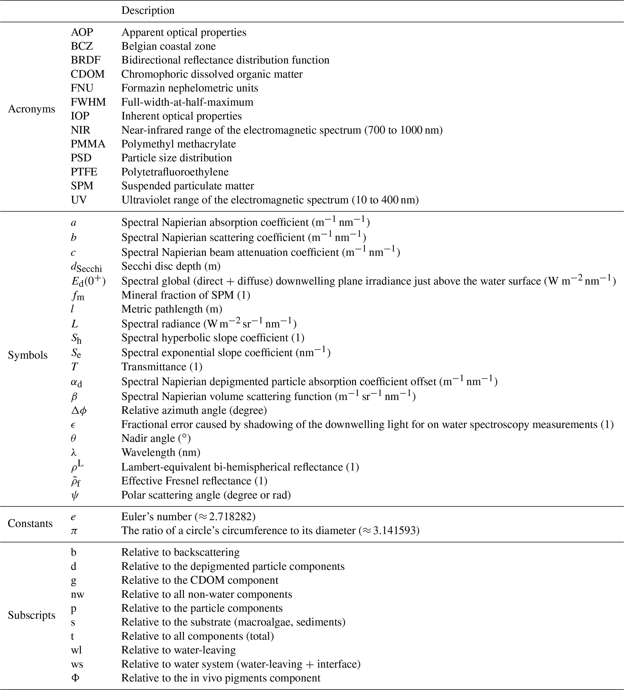
Measurements are presented in three groups: (1) inherent optical properties (IOPs) consisting of absorption, scattering and beam attenuation coefficients, near-forward volume scattering function, and turbidity; (2) apparent optical properties (AOPs) consisting of Secchi disc depth, water-leaving and substrate Lambert-equivalent bi-hemispherical reflectance; and (3) biogeochemical properties consisting of suspended particulate matter concentration, mineral fraction of particle mass, particle size distribution, pigment concentration, DNA metabarcoding, flow imaging microscopy counts, and bottom type classification. Table 1 presents a description of relevant acronyms, symbols, constants, and subscripts used in this study. The studied aquatic systems are listed in Table 2. The measured parameters and the number of samples are listed in Tables 3, 4, and 5. All coordinates are relative to the WGS84 datum and times are reported in UTC.
Linear models used for consistency check between parameters were fitted using robust linear regression (iterated reweighted least squares with Huber's loss function; Venables and Ripley, 2002). For selected parameters, the data summary is provided in the form of a violin plot, which, in addition to the median point and 25th and 75th percentiles, presents the empirical distribution of the data as the variable width of the planar shape. All analyses were performed in R (version 3.6.3, R Core Team, 2020) with aid of the packages “MASS” (version 7.3-51.5, Venables and Ripley, 2002), “vioplot” (version 0.3.6, Adler and Kelly, 2020), “dada2” (version 1.12.1, Callahan et al., 2016), and “decontam” (version 1.6.0, Davis et al., 2018).
2.1 Study sites
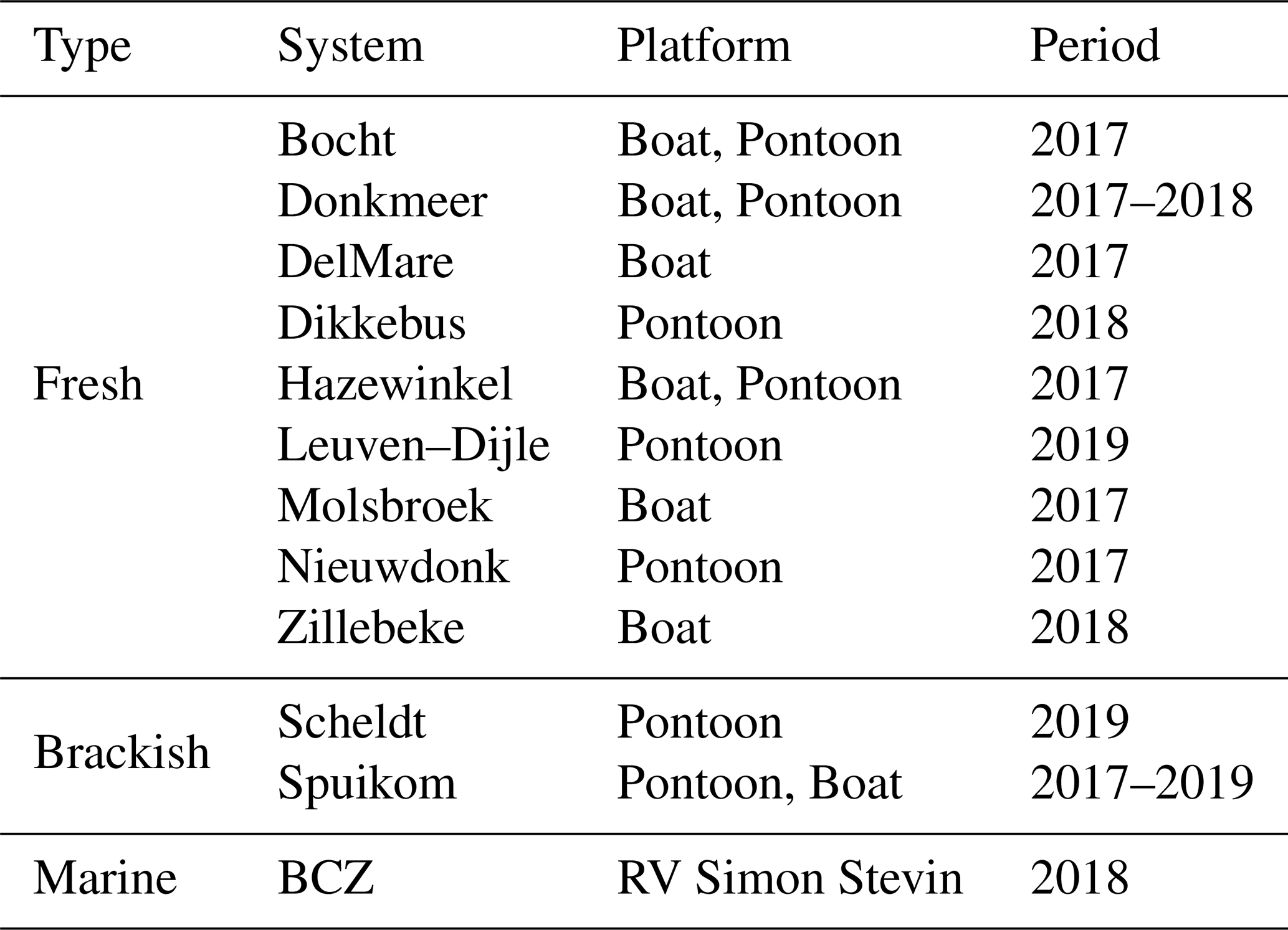
The majority of the measurements were performed in Belgian inland waters, in particular four lakes and a coastal lagoon. The sampling frequency during the growth season (spring to autumn) varied with the sampling year. The field campaigns were performed seasonally throughout 2017 (fortnightly) and 2018 (monthly), spanning a broad range of conditions. Data for four additional lakes with sporadic sampling during 2017 are also included in the dataset. Those systems were previously described in Castagna et al. (2020) and are reintroduced here for convenience. A summary of the study sites is presented in Table 2.
The Spuikom ( N E) is a shallow, brackish marine coastal lagoon (typical salinity between 27 and 33 PSU), with a surface area of 0.82 km2 and an average depth of 1.5 m. It is connected to the sea through the Ostend harbour by a lock system. The lagoon exchanges water with the harbour continuously, resulting in median daily renewal of 3.7 % of its volume. It is used for recreational activities and shellfish aquaculture. During the observation period (2017 to 2018), it experienced a cycle of diatom blooms in spring followed by a transition to transparent waters in autumn, with extensive bottom coverage by macroalgae. It is subject to strong coastal winds that can cause sediment resuspension, adding bottom sediments and benthic diatoms to the water column. The chlorophyll a (Chl a) concentration typically varied from 2 to 25 mg m−3, with the exception of an intense nanoflagellate bloom that reached a Chl a concentration of ≈ 130 mg m−3. The Secchi disc depth ranged from 0.62 m to bottom.
The Hazewinkel ( N E) is a mesotrophic lake with an area of 0.66 km2 and a maximum depth of 20 m. It is used for recreational and sports activities. During the observation period (2017), it presented a peak of phytoplankton abundance in spring, with Chl a concentration reaching 20 mg m−3, after which the concentration stayed around 5 mg m−3. Secchi disc depth varied from 1 to 6 m. Submerged macrophytes were confined to near-shore locations due to a steep basin slope.
The Donkmeer ( N E) is the second largest lake in Flanders, with a surface area of 0.86 km2 and an average depth of 2 m. It experiences recurrent cyanobacterial blooms of Anabaena spp. and Planktothrix agardhii (Descy et al., 2011). It is used for recreational activities and fishing. During the observation period (2017 to 2018), it experienced cyanobacterial blooms from summer to autumn, reaching a Chl a concentration of ≈ 400 mg m−3 and a Secchi disc depth of 0.2 m. Its northern and southern portions are connected through a narrow and shallow passage, with the northern portion experiencing a shorter period of cyanobacterial blooms due to management actions.
The Dikkebus ( N E; 0.36 km2, 2.5 m deep) and the Zillebeke ( N E; 0.28 km2, 2 m deep) are two lakes created in the 13th century for water supply, a function that remains to date along with recreational activities. Both lakes exhibit annual blooms of the cyanobacteria Microcystis aeruginosa and Aphanizomenon flos-aquae (Descy et al., 2011). During the observation period (2018), intense cyanobacterial blooms were observed, with the Chl a concentration reaching 105 mg m−3; in the Zillebeke, these blooms were associated with fish mortality. The Secchi disc depth ranged from 0.5 to 2 m. Additional stations were included from four other Flemish lakes: Bocht ( N E; 0.35 km2 and 18 m deep), Nieuwdonk ( N E; 0.26 km2 and 22 m deep), and two unnamed adjacent lakes ( N E; ≈ 0.16 km2 each and 10 m deep), here referred to as “DelMare”, a sand-extraction lake with water sports activities, and “Molsbroek”, a nature reserve.
Other inland water systems included were the Scheldt estuary and the Leuven–Dijle canal. The Scheldt is a rain-fed lowland river, with an estuary environment subjected to tides from the mouth at Vlissingen (the Netherlands) to Ghent (Belgium, 160 km upstream), where a system of locks prevent further propagation of the tide (Meire et al., 2005). It has high economical importance as a transport waterway, connecting the harbours of Antwerp and Ghent to the North Sea. The Scheldt estuary was sampled in mid-October 2019 at two locations near the city of Sint-Amands ( N E and N, 4 E), with a time series including a full tidal cycle (tidal range of 6 m). During the observation period, the Chl a concentration reached 55.7 mg m−3 at high tide, while the suspended particulate matter (SPM) concentration reached 791.2 g m−3. In the same campaign performed in the Scheldt, two samples were taken at the Leuven–Dijle canal, a highly transparent artificial waterway running parallel to the Dijle river, connecting Leuven to the Zenne–Dijle confluence and, ultimately, to the Scheldt. The sampling position was close to the lock of Zennegat (N E).
The stations sampled in the BCZ are part of the regular LifeWatch sampling campaigns (Mortelmans et al., 2019). The April and July 2018 campaigns were augmented to include spectroscopic measurements. The BCZ is a shallow part of the North Sea (1 to 40 m), experiencing high tidal fluctuations (average of 4 m) and strong tidal currents (1 m s−1). Those conditions, combined with limited freshwater discharge into the region, result in a well-mixed water column (van Beusekom and Diel-Christiansen, 1994). It experiences high turbidity (SPM concentration from 1 to 200 g m−3) with a large influence from particulate material imported through the Strait of Dover (Fettweis and Van den Eynde, 2003). The BCZ develops a turbidity maximum zone near Zeebbrugge, also influenced by the decreasing magnitude of the residual transport vectors from the eastern border (Fettweis and Van den Eynde, 2003). The inflow of the Yser and Scheldt rivers influences the availability of nutrients, with an increase of nitrogen and phosphorus since the second half of the 20th century, followed by a de-eutrophication phase during which nitrogen and especially phosphorus decreased (Desmit et al., 2020). The phytoplankton seasonal dynamics are well described (e.g. Reid et al., 1990), with an early spring diatom bloom followed by a mixed bloom of the haptophyte Phaeocystis globosa and diatoms. A recent review of the phytoplankton seasonal dynamic was provided by Castagna et al. (2021). The IOPs in this region were extensively studied by Astoreca et al. (2006, 2009, 2012).
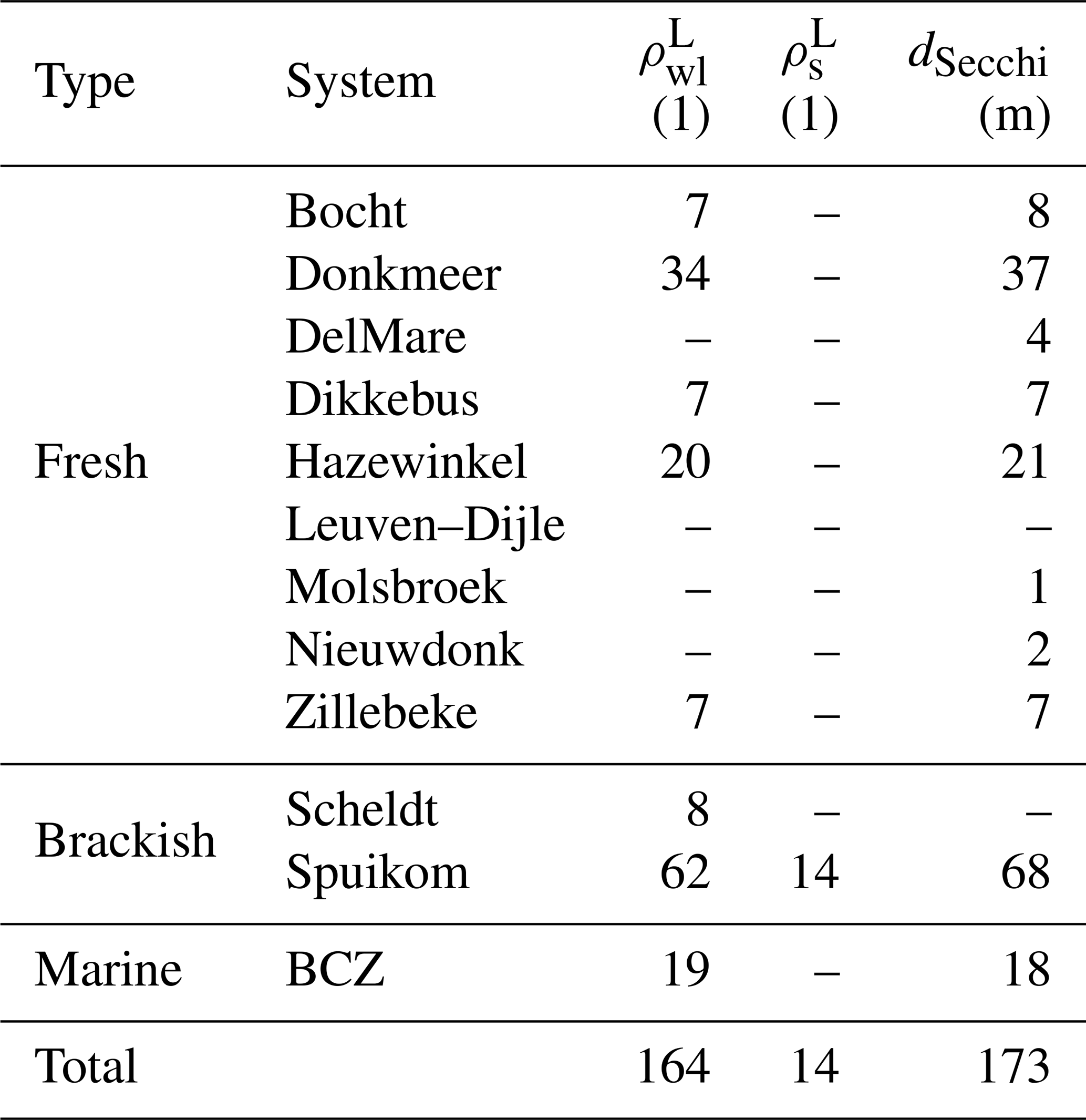
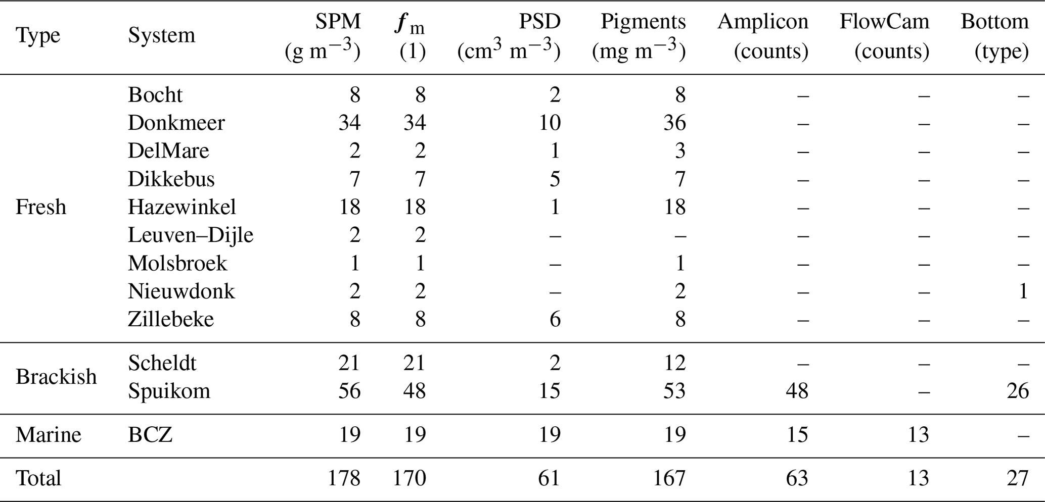
Table 2Summary of Belgian water systems sampled in this study.
2.2 Sampling
Sampling was performed from a diverse set of platforms. For the inland water campaigns, samples were taken from pontoons or an inflatable boat, depending on the system and date. The water was sampled just below the surface, taking care not to draw in materials floating at the surface (e.g. pollen, debris, etc.). Field samples were stored in 5 L semi-transparent plastic carboys, kept in the dark and cold during transport to the laboratory, and processed within 4 to 6 h of sampling. Sampling for the coastal campaigns was performed from the Research Vessel (RV) Simon Stevin (Flanders Marine Institute, VLIZ). For most marine samples, water was sampled just below the surface using Niskin bottles (General Oceanics, Inc.) attached to a rosette system. Subsurface samples for flow imaging microscopy were the exception, taken with a bucket from the side of the ship. Filtrations were performed on board and water subsamples were kept in the dark and cold during transport to the laboratory for spectrophotometric measurements.
Macrophytes, sediment, and biofilm were sampled in the Spuikom lagoon. Macrophytes were sampled during 2017 and 2018 by collecting floating specimens or recovering specimens from the bottom using a rake. Specimens were stored in transparent plastic bags containing water from the lagoon, and kept in the dark and cold during transport to the laboratory. Sediments and biofilm were sampled in April 2018 using polymethyl methacrylate (PMMA) tubes attached to a short corer. The cores were retrieved with care so as not to disturb the surface of the sediment, sealed, and transported to the laboratory in a vertical position. In July 2018, biofilm patches had detached from the bottom of the Spuikom and were sampled floating at the surface and stored in plastic bags for microscopic examination. The cores and macrophytes were stored in a climate room at 4 ∘C for up to 3 d until analysis.
2.3 Inherent optical properties
Most of the IOP measurements were performed ex situ with a benchtop spectrophotometer (Lambda 650S, PerkinElmer) equipped with an integrating sphere (150 mm internal diameter). The interior of the integrating sphere is made of highly reflective (nominally 99 %) sintered polytetrafluoroethylene (PTFE). The spectral IOP measurements made with the spectrophotometer include particle absorption (ap), chemically decomposed into in vivo pigment absorption (aΦ) and depigmented particle absorption (ad), and chromophoric dissolved organic matter absorption (ag), particle beam attenuation (cp), and scattering (bp) Napierian coefficients. Methods followed recommendations from Pegau et al. (2002) and IOCCG (2018). Measurements covered the range from 250 to 850 nm in 1 nm steps, with a 2 nm integration slit and 0.24 s integration time (250 nm min−1). Data are provided in the range of 380 to 850 nm, and include a single pass of a smoothing function to reduce noise (rectangular filter, 10 nm window moving average).
Turbidity, defined as the side-scattering at 860 nm relative to Formazin standards (ISO 7027:1999, 1999; Dogliotti et al., 2015; Boss et al., 2009a), was measured in discrete samples with a portable turbidimeter (2100P ISO, HACH). Additional IOP data were measured using in situ instrumentation for a subset of water systems and stations. These include the diffraction peak (ψ< 15∘) of the particle volume scattering function (VSF; βp(670)) and non-water beam attenuation at an acceptance angle of 0.018∘ measured at 670 nm (cnw(670,0.018); LISST, Sequoia Scientific).
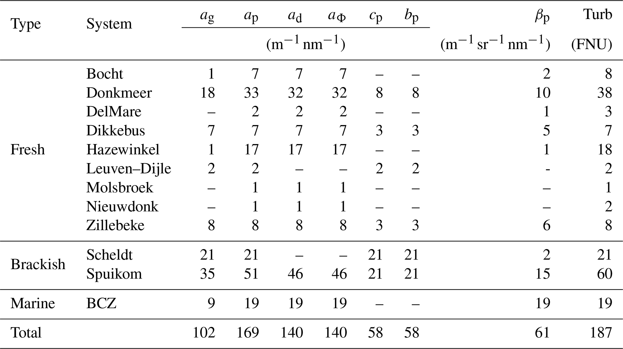
Table 3Summary of measured and derived inherent optical properties per water system. Values indicate the number of valid, quality-checked measurements.
2.3.1 Absorption coefficient from dissolved components (<0.45 µm)
Absorption due to chromophoric dissolved organic matter (CDOM) was determined in the laboratory from fresh and undiluted filtered subsamples, using a 5 cm pathlength quartz cuvette. Subsamples were filtered with 0.45 µm polyamide (nylon) fibre syringe filters. Between samples, the syringe and cuvette were rinsed with deionised water. The filters were first rinsed by filtrating 15 mL of deionised water before use with samples. The first sample filtration volume was used for final rinse of the quartz cuvette and the volume discarded. The cuvette was then gently filled with the second filtration volume to avoid formation of bubbles, and allowed to rest for at least 3 min before measurements. The blank was determined with deionised water, using the same cuvette and at the same temperature (room temperature ≈ 20 ∘C). Quality control evaluated the presence of absorption peaks at 676 nm as an indication of cell leakage and the offset from zero absorption at 750 nm as a indication of the presence of hydrosols.
The use of deionised water as a blank for all measurements resulted in a mismatch of salinity for marine and brackish samples. Dissolved salts change the complex refractive index of water (Quan and Fry, 1995; Röttgers et al., 2014b), affecting reflection and refraction interactions with the cuvette wall, water scattering, and absorption. In the wavelength range reported here, the scattering effects and the absorption of salts are negligible; however, the dissolved salts form what is known as salt-solvated water, mixed with pure water (Max and Chapados, 2001). Salt-solvated water can have higher or lower absorption than pure water, depending on the wavelength, with a magnitude defined by the salt type (Max and Chapados, 2001; Röttgers et al., 2014b). This difference is particularly important in the NIR range, due to the spectral shape of ag. The effect of the mismatch in salinity was investigated by comparing the effects of salinity on blank readings for ag determinations from deionised water and artificial seawater at a salinity of 35 (NaCl at 35 g kg−1). The results are shown in Fig. S1 in the Supplement, and the resulting difference spectrum was subtracted from ag of the Spuikom lagoon and the BCZ for an approximate correction. Dissolved molecular oxygen (O2) also contributes to absorption in the UV range (Jonaz and Fournier, 2007, and references therein); however, in the wavelength range reported here, CDOM dominates the signal.
The Lambda 650S was not available in 2017 and ag was measured for a subset of samples using another spectrophotometer (UV-1601, Shimadzu). Sample preparation was the same, except that ag was only measured at selected wavelengths (380, 400, 433, 550, and 750 nm). To retrieve the full spectrum for these samples, a hyperbolic model was fitted to the available wavelengths (Twardowski et al., 2004). The hyperbolic model fit was also applied to all measurements in the range of 380 to 850 nm to provide a smooth, fitted version of ag and to calculate the CDOM absorption spectral hyperbolic slope coefficient, :
Most samples had negligible absorption in the NIR range (< ), fluctuating around zero due to instrument noise or a residual blank salinity difference effect. Four stations had positive or negative offsets that were larger than , and the negative offsets were attributed to the presence of bubbles in the blank of the day. The average ag between 750 and 850 nm was subtracted from all spectra. Five freshwater samples had a pronounced Chl a absorption peak at 676 nm, and since NIR signals were close to zero, those peaks likely resulted from cell leakage. The ag values for those stations were flagged.
The magnitudes of ag(412) varied between 0.547 and 4.185 , with values above 2.25 generally observed only in freshwater systems. The exception was a sample in the Spuikom collected during a nanoflagellate bloom, when ag(412) reached 3.160 . The range of the was between 5.60 and 8.81. The observed values of ag and fitted are presented in Fig. 1.
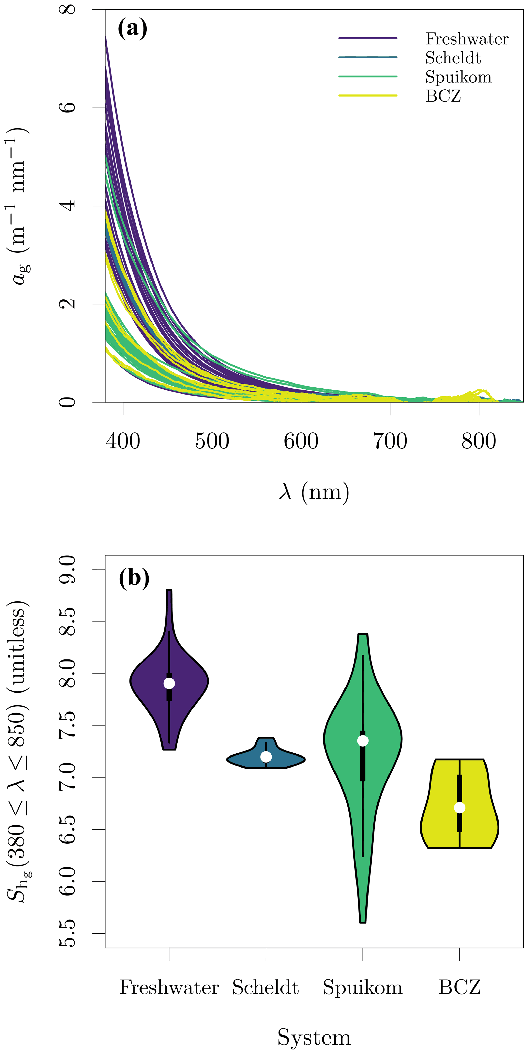
Figure 1Chromophoric dissolved organic matter (CDOM) absorption in the Belgian water systems. (a) CDOM spectral absorption coefficient, ag; and (b) hyperbolic slope of ag, , fitted in the range of 380 to 850 nm.
2.3.2 Absorption coefficient from particulate components (> 0.7 µm)
Particle absorption was measured using the filterpad method, with particles concentrated onto a glass fibre filter (GF/F, effective mesh of 0.7 µm). To improve the homogeneity of particle deposition over the filtration area, two stacked filters were used and samples with a high abundance of particles were diluted in the filtration funnel with deionised water. Immediately after filtration, filters were transferred to PetriSlides (Merck), wrapped in aluminium foil, and frozen in liquid nitrogen. Filters were then stored at −80 ∘C until analysis.
Before analysis, the filters were allowed to thaw to room temperature and kept hydrated with deionised water. To avoid dislocating large particles deposited on the filter fibres, hydration was performed by raising the filter, adding a droplet of water to the PetriSlide base, and gently lowering the filter onto the droplet, resulting in water spreading by capillarity. The “inside sphere” variant of the quantitative filterpad method was used (Stramski et al., 2015), using a centre mount coated with PTFE. Filters were read twice, with a 90∘ rotation between reads to average small deviations from homogeneous deposition. This was especially important to account for large cyanobacteria colonies when these occurred at low densities (Fig. S2 in the Supplement). Pigments were then oxidised by treating the filters with sodium hypochlorite (NaClO; Ferrari and Tassan, 1999), using the same approach as for hydration. Filters were read after 15 min or complete oxidation, following the same orientations as of the pigmented readings. The pathlength amplification correction was taken from Stramski et al. (2015) as recommended in IOCCG (2018). The in vivo pigment absorption coefficient (aΦ) was calculated as the total particulate absorption coefficient (ap) minus the depigmented particle absorption coefficient (ad). The chemical oxidation step was not performed for the Scheldt samples.
Sodium hypochlorite has an absorption peak at ≈ 300 nm, with residual absorption up to 500 nm. One method to remove the oxidant's signal is to rinse the filter with pure water before determination of ad and this method was used for a subset of samples to evaluate the impact of sodium hypochlorite and rinsing. We observed that some samples had an apparent loss of ad observed between determinations with sodium hypochlorite and after rinsing (Fig. 2). The magnitude of this effect varied across the lakes, with Spuikom, Donkmeer, Hazewinkel, and Bocht suffering little to no loss between 550 and 850 nm, while Dikkebus and Zillebeke showed large reductions in ad after rinsing. This effect might provide additional information on the nature of the particles in a given system, but needs to be further explored to understand its causes. A direct consequence for measurements of ad and aΦ is that rinsing might underestimate ad.
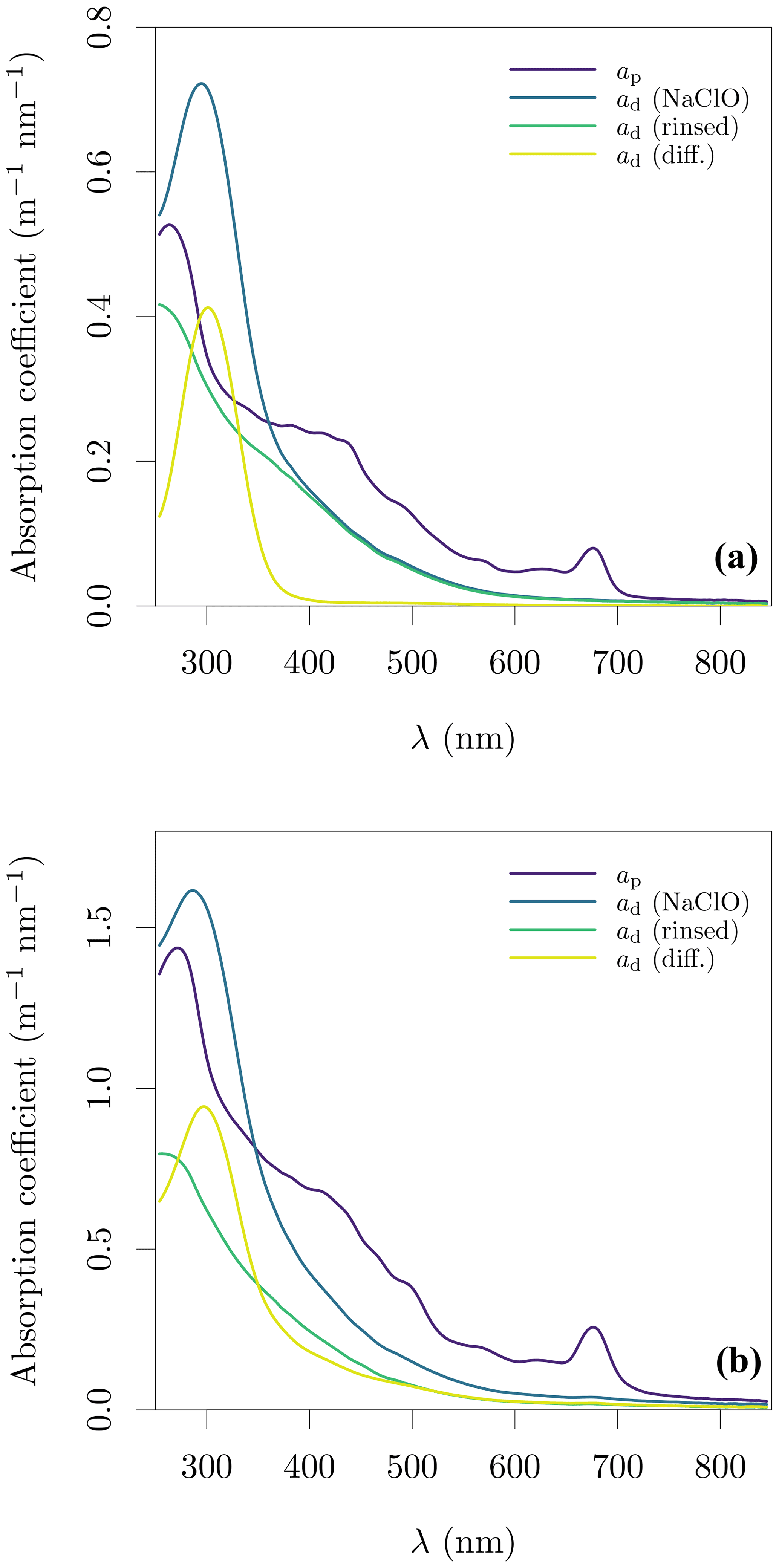
Figure 2Evaluation of the treatment of filters with sodium hypochlorite (NaClO) and subsequent rinse on the determination of ad. (a) A sample from the Bocht (BL_08) and (b) a sample from the Dikkebus (DK_01). The sample in panel (b) shows loss of absorbing material after rinsing.
Therefore we developed a statistical method to remove the oxidant's signal, instead of applying rinsing. We observed that when there was no loss of signal with rinsing, the minimum difference between ap and rinsed ad in the UV range was at 305 nm, with ad(305) typically between 80 % and 90 % of ap(305) (Fig. 2a). Based on these observations, we fitted an exponential function to the measured ad with sodium hypochlorite in the range of 550 to 850 nm, and included a point-estimate of rinsed ad at 305 nm as 0.8ap(305). The additional data point at 305 nm helps to set the curvature of the exponential model. Finally, an offset was included as necessary to match the ap absorption in the NIR end. The exponential model with an offset was
where αd () is a spectrally flat offset (Estapa et al., 2012) and (nm−1) is the spectral exponential slope of ad.
The treatment with sodium hypochlorite can also introduce another artefact to the measurements. For a set of samples we observed a baseline offset between ap and ad in the NIR range even before rinsing, propagating to increased baseline absorption of aΦ. This likely results from sodium hypochlorite removing the adsorbed organic layer over particles (Binding et al., 2008), with the magnitude of the effect proportional to the concentration of particles and organic matter. In our samples, this effect was larger in the maximum turbidity zone of the BCZ. This loss of absorbing material was not observed in a study by Röttgers et al. (2014a) including samples from a diverse set of environments, although the authors did not apply NaClO to the North Sea or Baltic Sea samples. The baseline effect was compensated for by adding the minimum offset necessary to match ap and ad in the range of 800 to 850 nm without generating negative aΦ values. This constant offset likely underestimates the contribution of organic absorption in the blue end due to the exponential spectral shape of this component (e.g. Cael and Boss, 2017).
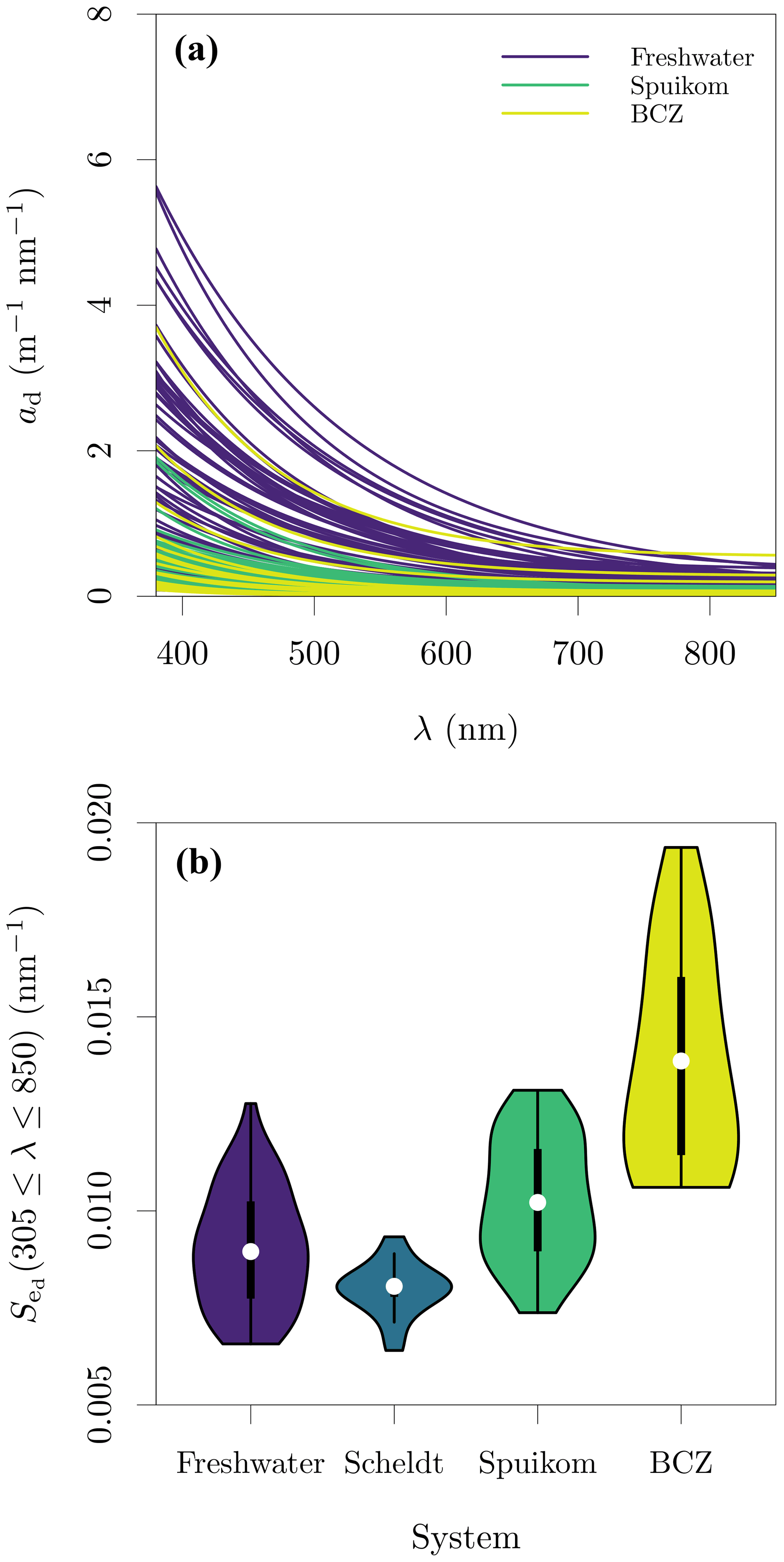
Figure 3Depigmented particle absorption in the Belgian water systems. (a) Fitted depigmented particle absorption coefficient, ad; and (b) spectral exponential slope of ad, , fitted in the range of 380 to 850 nm. Note that for the Scheldt samples, the exponential model was fitted directly to ap.
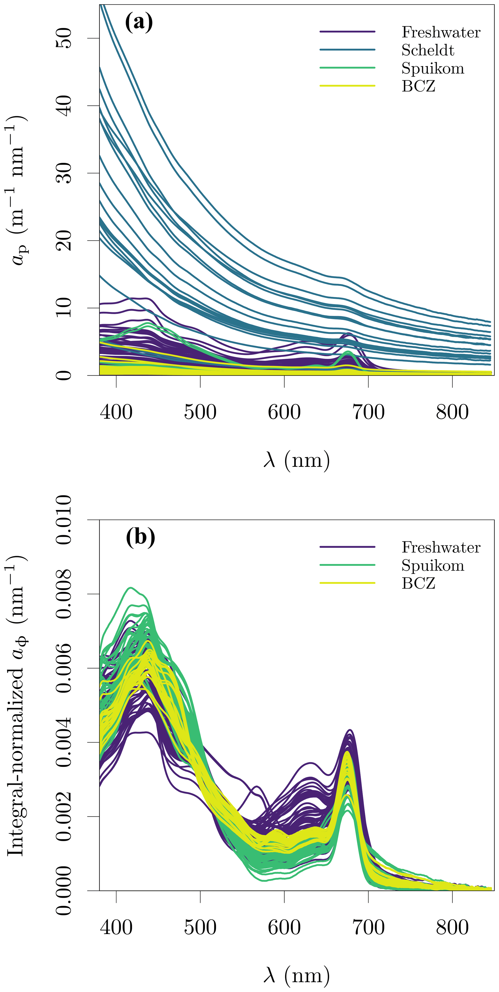
Figure 4Particle and in vivo pigment absorption in the Belgian water systems. (a) Particle absorption coefficient, ap; and (b) in vivo pigment absorption coefficient, aΦ. The aΦ presented here was calculated with the fitted ad.
Similar to what was observed for ag(412), the magnitude of ad(412) varied between 0.055 and 4.570 , with values above 2.79 generally observed only in freshwater systems. The baseline absorption coefficient in the NIR range (ap or ad, and equal to aα) ranged from 0.003 to 7.933 , with only Scheldt samples presenting values higher than 0.565 . The range of was between 0.0064 and 0.0194 nm−1. The fitted values of ad and are presented in Fig. 3. Since particle-absorption samples from the Scheldt were not depigmented but were dominated by ad (Fig. 4a), an estimate of is provided by fitting Eq. (2) directly to ap (Fig. 3b).
The integral-normalised aΦ presented a diversity of pigment absorption peaks (Fig. 4b), showing spectral shapes associated with dominance of cyanobacteria and green and red lineages of algae. Considering that aΦ was retrieved from fitted ad, an independent validation was performed against the total Chl a concentration (described later). In the blue end of the spectrum, we used Gaussian decomposition (Hoepffner and Sathyendranath, 1991; Chase et al., 2013) to extract the magnitude associated with the Soret band of Chl a in vivo (435 nm; Fig. 5a). In the red end of the spectrum, we compared aΦ(676) against models fitted to global datasets (Nardelli and Twardowski, 2016, Fig. 5b). We note that our observations are similar to those reported by Hoepffner and Sathyendranath (1991), while the values of Nardelli and Twardowski (2016) are lower, likely due a combination of their lower Chl a concentration range and their estimation of aΦ(676) from the line height (Roesler and Barnard, 2013). The median spectral mass-specific in vivo pigment absorption coefficient at 676 nm, ∗aΦ(676), was equal to 0.022 (Fig. 5c), similar to the value of 0.020 presented by Hoepffner and Sathyendranath (1991). In the comparisons in the blue and red spectral regions, we observe a linearity in log scale, with larger spread in the comparison aGauss(435) likely due to a combination of uncertainty in the estimate of the fitted ad and the variable pigment packaging effect (Morel and Bricaud, 1981; Latimer, 1983), both larger in the blue spectral range.
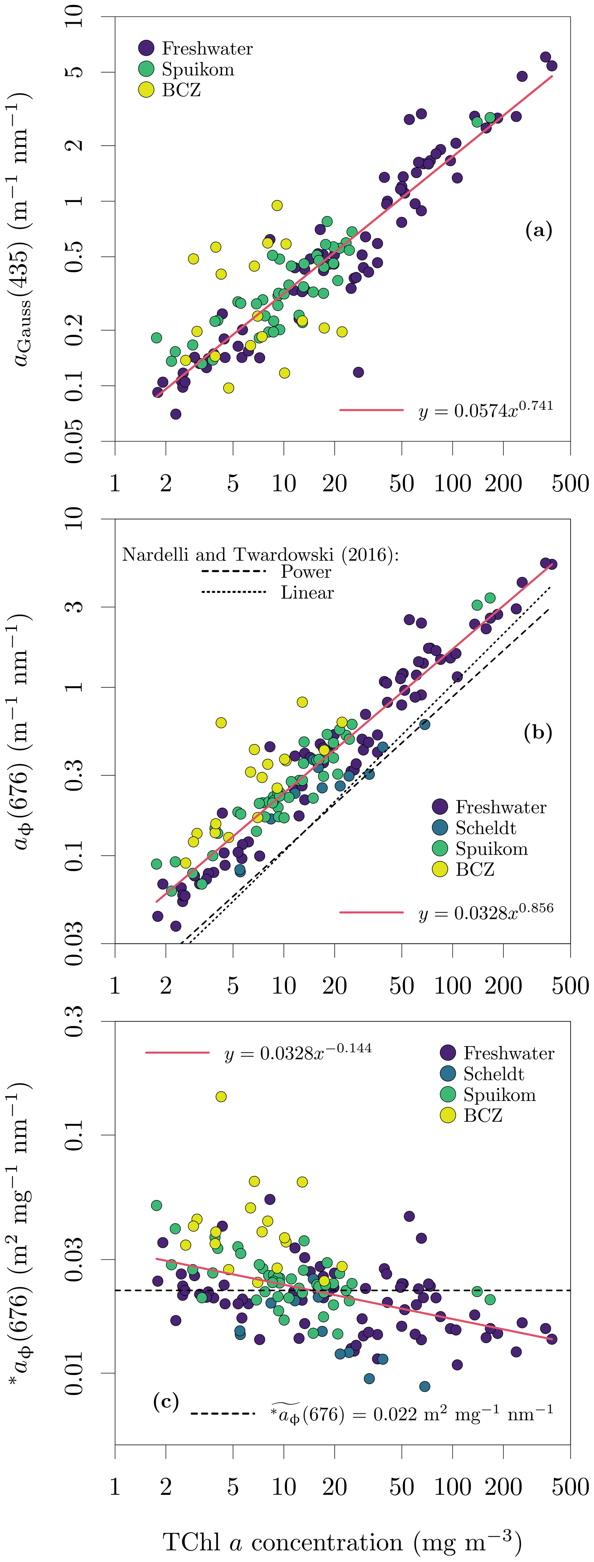
Figure 5Relation between the total chlorophyll a (monovinyl chlorophyll a + chlorophyllide a) and in vivo pigment absorption. (a) Magnitude of the Gaussian peak centred at 435 nm; (b) the in vivo pigment absorption at 676 nm, aΦ(676); and (c) mass-specific in vivo pigment absorption at 676 nm, ∗aΦ(676). The aΦ(676) for the Scheldt samples was estimated as the line height (Roesler and Barnard, 2013).
2.3.3 Near-forward (< 15∘) particle volume scattering function
The near-forward particle volume scattering function (VSF; βp) at 670 nm was measured with two Laser In-Situ Scattering and Transmissometery (LISST, Sequoia Scientific Inc.) instruments, models 200X and 100X, equipped with a type C detector . The LISST-100X has a set of 32 concentric detectors measuring βp between 0.038 and 7.519∘, while the LISST-200X has a set of 36 concentric detectors, the first 32 detectors measuring βp between 0.081 and 15.394∘. Single-depth measurements were taken at 1 m depth, with the instrument deployed horizontally (LISST-200X) or vertically (LISST-100X), having the optical sensor end oriented downward. The vertical deployment, preferentially made on the shady side of the platform, was chosen to reduce the interference of environmental light, since the model 100X does not compensate for external light. Considering those deployment conditions and that our systems were mostly turbid, we expect a negligible influence of environmental light on the measurements. The instruments were used in a subset of stations. Calibrations with deionised water were performed monthly and the most recent calibration used for blank values. The VSF was retrieved from the raw LISST data file, using the procedures described in Agrawal (2005) and the instrument calibration files.
Quality control was performed by flagging entries in which the single scattering transmittance (Tb) was lower than 30 %, to avoid artefacts produced by multiple scattering:
where bt is the total scattering coefficient and lLISST is the pathlength of the LISST instrument. The non-water beam attenuation coefficient at 670 nm measured by the LISST transmittance sensor with an acceptance angle of 0.018∘, cnw(670,0.018), was subtracted by the anw(670) measured with a benchtop spectrophotometer to calculate bt(670,0.018). The VSF is an important parameter for a tentative correction of the spectral particle beam attenuation and scattering coefficients measured with the benchtop spectrophotometer.
2.3.4 Beam attenuation and scattering from particulate components (> 0.45 µm)
In addition to cnw(670,0.018) measured by the LISST instruments, the spectral particle beam attenuation (cp) and scattering (bp) coefficients were calculated from cnw measured on fresh samples with the Lambda 650S spectrophotometer, by subtracting ag and ag+ap, respectively. To reduce the acceptance angle of the spectrophotometer (Boss et al., 2009b; Leymarie et al., 2010), a black barrier with a central circular aperture of 2.4 mm diameter was placed in the entry port of the integrating sphere. With a distance of 69.5 cm from the centre of the sample cell to the integrating sphere (due to system of mirrors extending the pathlength), the detector acceptance angle in water for this configuration is 0.074∘. The integration time of the instrument was increased to 0.4 s (150 nm min−1) to compensate for the reduced signal, but noise levels were still noticed throughout the spectra. On later samples, the reference beam was partially blocked with a 1 % transmittance filter to reduce the dynamic range imposed by the lack of a similar aperture in the reference beam.
As with ag, cnw was measured in undiluted water subsamples, using 1, 5, or 10 cm quartz cuvettes, depending on the turbidity. Blank readings were measured with deionised water, resulting in mismatched salinity for brackish and marine samples. The effect of the mismatched salinity was evaluated by comparing the beam attenuation between deionised water and artificial seawater at a salinity of 35 (NaCl at 35 g L−1) in the same experimental conditions as sample measurements. In the range from 380 to 850 nm, the difference in beam attenuation coefficient was ≈ 0.12 (Fig. S3 in the Supplement). The difference spectrum was subtracted from all brackish and marine samples for an approximate correction.
The measurements of cp(670,0.074) made with the benchtop spectrophotometer were tested against the LISST determinations of cp(670,0.018), with a similar method to that described in Boss et al. (2009b). Measurements of cnw from both instruments were converted to cp by removing the absorption by CDOM at 670 nm. The difference between cp(670) estimated by each instrument should be accounted for by the additional scattering signal captured by the larger acceptance angle of the spectrophotometer, given by integration of the VSF between 0.018 and 0.074∘. The VSF between the lowest angle measured by the LISST (0.038∘ or 0.081∘) and its transmittance acceptance angle (0.018∘) was calculated with linear extrapolation in log 10 space from the two lowest measured angles. A detailed demonstration for sample DN_29 is presented in Fig. S4 in the Supplement. Figure 6a shows the result for all samples with paired data available, with data closely following the 1:1 line, and variation possibly caused by artefacts related to in situ versus ex situ measurements. This analysis validates the cp measurements with the spectrophotometer.
The additive error due to contamination with the near-forward scattered signal within the acceptance angle can be accurately corrected for only when the VSF of each sample is known. However, an approximate correction is possible. Figure 6b shows that the scattering signal in the range of 0.018 to 0.074∘ represents an average of 43.2 % of the particle scattering coefficient, with a stable relation across systems and seasons. Assuming that the angular shape of the VSF presents minor spectral variability and that the VSFs of different systems and seasons in our dataset are well represented by the subset for which LISST data are available, it is possible to use the approximate correction:
The LISST-equivalent (acceptance angle of 0.018∘) version of the spectral bp and cp are also provided in conjunction with the measured values (acceptance angle of 0.074∘), as recommended by IOCCG (2018).
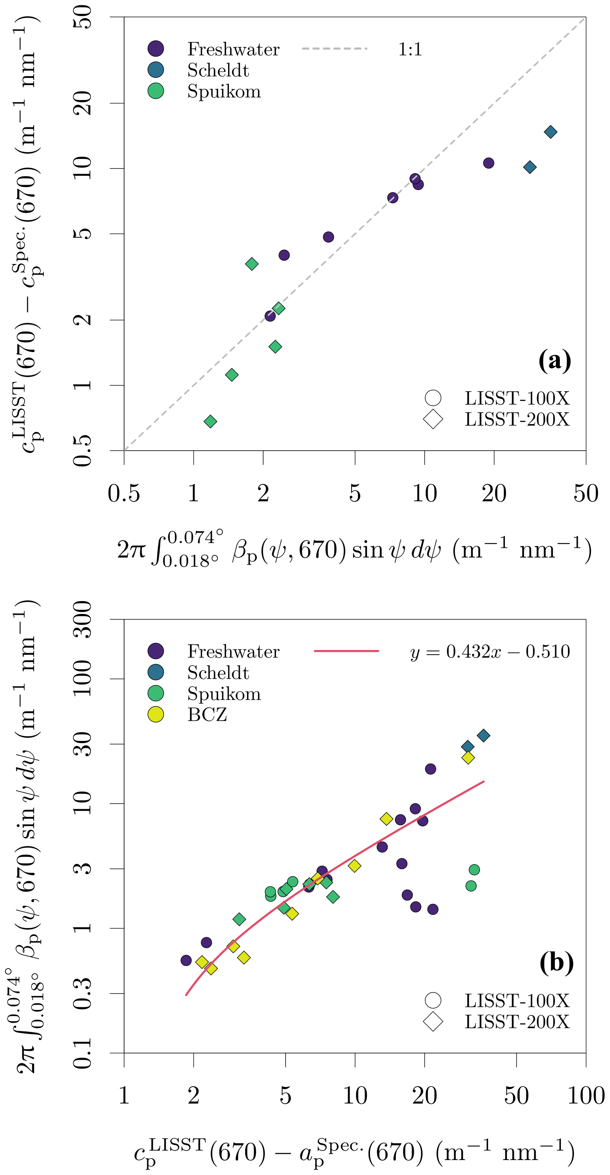
Figure 6Evaluation of cp measurement bias due to the finite acceptance of the spectrophotometer. (a) Relation between the difference of the cp measured with the spectrophotometer and the LISST, and the VSF integral in the range of solid angles defined by the difference of their acceptance angles. (b) Relation between the scattering coefficient () and the magnitude of scattering between 0.018 and 0.074∘ scattering angles (ψ).
Quality control included flagging of cp spectra showing irregular behaviour. Particle beam attenuation is a smooth spectral function (Roesler and Boss, 2003) due to anomalous diffraction that causes a complementary pattern between scattering and absorption (Zaneveld and Kitchen, 1995). Disturbances can be present in the form of small peaks caused by pigment absorption, or oscillations caused by anomalous dispersion when there is a large contribution of small particles to the beam attenuation, but their shape and position are characteristic. Large, abrupt, and otherwise irregular spectral behaviour likely arises from motion of large particles in the beam cross sectional area. Six samples from Belgian lakes were flagged by this procedure, all with the presence of large cyanobacteria aggregates. All BCZ samples from April, taken during a major Phaeocystis bloom, were also discarded due to similar effects of the large colonies. Beam attenuation remains elusive for standard benchtop spectrophotometric analysis (sequential spectral scanning) under these conditions. As an example, cyanobacteria aggregates were observed floating on the surface of the cuvette at the end of the spectral run, even though the samples were mixed at the start of the measurement.
Another source of bias related to beam attenuation measurements in a spectrophotometer is that total internal reflection will occur for a fraction of the scattered light, dependent on the incident angles on the water side of the quartz wall. Some fraction of the internally reflected light could scatter back into directions in the detector's acceptance angle and artificially decrease beam attenuation measurements (IOCCG, 2018). Our experimental procedure did not include a dark baffle inside the cuvette to reduce this potential effect. Finally, our measurements show an oscillation centred at ≈ 500 nm, regardless of system, particle type, or concentration. This suggests that this oscillation is an artefact of the measurement procedure, though we could not identify its source. The spectral (LISST-equivalent) beam attenuation and particle scattering coefficients are presented in Fig. 7
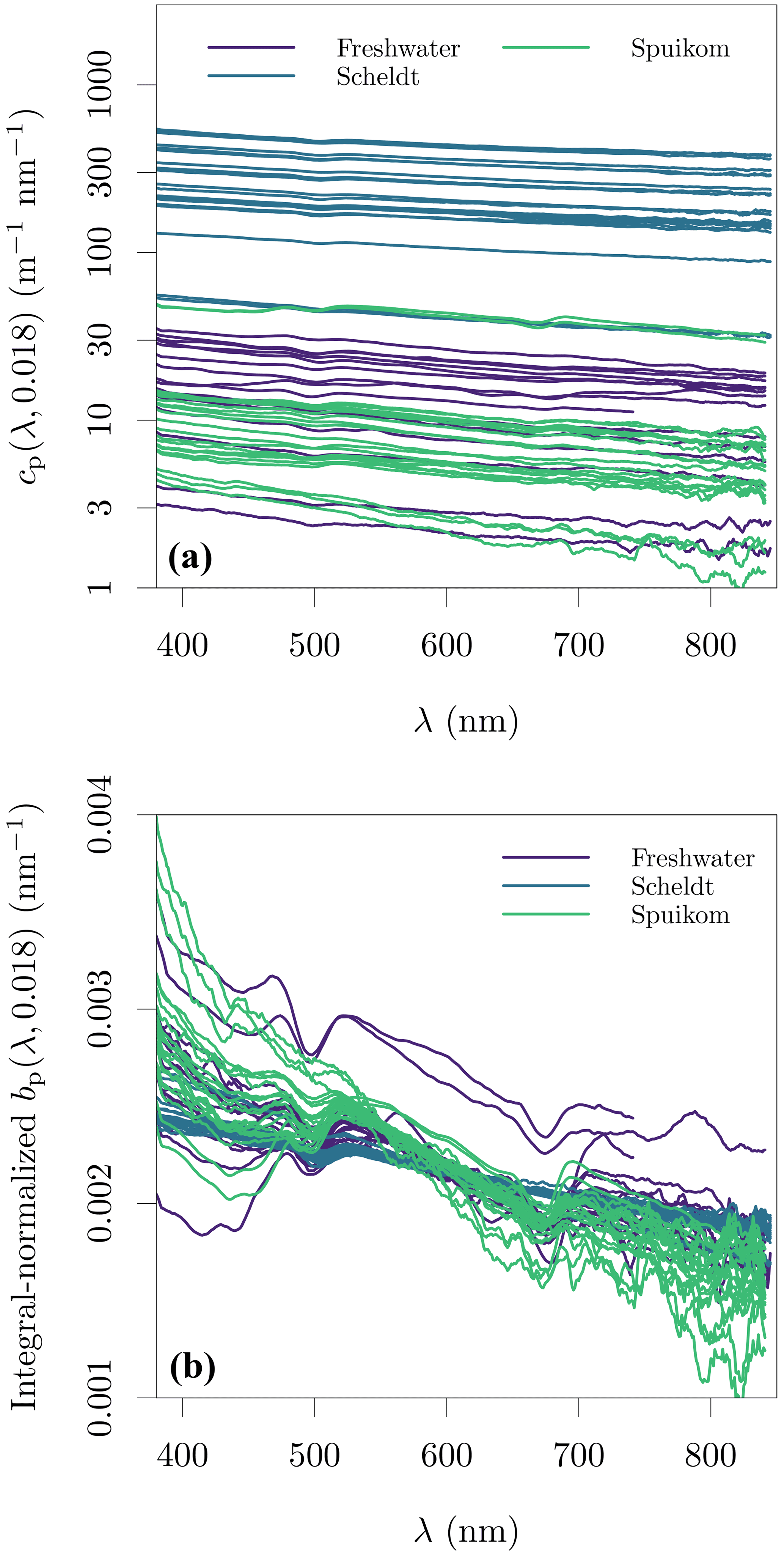
Figure 7LISST-equivalent (acceptance angle of 0.018∘) spectral particle beam attenuation coefficient, cp (a), and integral-normalised particle scattering coefficient, bp (b).
2.3.5 Turbidity
Turbidity was quantified as formazin nephelometric units (FNU), a NIR side-scattering (90∘) VSF magnitude relative to formazin standards. For the BCZ and Scheldt campaigns, turbidity was measured just after water sampling, while for the lakes and lagoon, the turbidity was measured after transportation to the laboratory. The transportation might result in changes in particle aggregation due to changes in turbulence. However, we found a single linear relation between turbidity and suspended particulate matter (described later in Sect. 2.5.1) across all systems and seasons.
2.4 Apparent optical properties
The AOP measured in situ were Secchi disc depth (dSecchi) and the Lambert-equivalent water-leaving bi-hemispherical reflectance (). The was measured with the above water or on-water protocols, depending on the system. The Lambert-equivalent bi-hemispherical reflectance () measurements of substrate samples (sediments, macroalgae) were performed ex situ, underwater and in air, using natural illumination.
The “Lambert-equivalent” qualification indicates that the bi-directional reflectance distribution function (BRDF) of the targets is assumed to be well represented by the Lambert model, and the hemispherical-directional measurement is converted to bi-hemispherical by scaling it with the cosine-weighted solid angle integral of a hemisphere, π sr. The water-leaving signal is not strictly Lambertian; however, this approximation is commonly used for remote sensing purposes (Frouin et al., 2019).
Table 4Summary of measured apparent optical properties per water system.
2.4.1 Secchi disc depth
A standard quadrant Secchi disc (black and white, 30 cm diameter) was used to measure transparency. The Secchi disc was deployed from the shady side of the sampling platform, recording the depths of disappearance and reappearance. The Secchi disc depth (dSecchi) was recorded as the average of the two depths. A tentative correction for the effect of sun zenith angle (described later) at the time of measurement (Lee et al., 2015) was applied following the formulation of Verschuur (1997). This correction normalises the Secchi disc depth measurements to the sun at the zenith. Measured and corrected values are provided. A comparison between turbidity and the inverse Secchi disc depth, corrected for the sun zenith angle, shows a log-linear relation and is presented in Fig. S5 in the Supplement.
2.4.2 Lambert-equivalent water-leaving bi-hemispherical reflectance
Reflectance spectroscopy measurements were performed in Belgian lakes and the coastal lagoon using the “on-water” method, also known as the skylight-blocked approach (Lee et al., 2013, 2019; Ruddick et al., 2019b). Measurements were made with a handheld spectrometer (FieldSpec HH, Analytical Spectral Devices) equipped with 7.5∘ field-of-view (FOV) foreoptics. The instrument has bands with 3.6 nm full width at half maximum (FWHM) and a spectral sampling of 1.6 nm, covering the range from 325 to 1075 nm. Water-leaving radiance (Lwl) was recorded at 0.5 m horizontal distance from the deployment platform, aligned with the sun azimuth, and with the opening of the lens' cylindrical shield 2.5 cm below the water surface. The global downwelling plane irradiance just above the surface (Ed(0+)) was estimated from near-coincident measurements of the exitant radiance of a sintered PTFE reference target (nominal reflectivity of 12 %) held parallel to the surface (Castagna et al., 2019; Ruddick et al., 2019a). An example of the measurement approach is presented in Fig. S6 in the Supplement. A total of 10 Lwl spectra and 5 plaque exitant radiance spectra were averaged per station, with the measurement sequence completed within 2 min. The Lambert-equivalent water-leaving bi-hemispherical reflectance () was estimated according to
where ϵ is the estimated fractional shadowing error from the instrument and platform, θ is the nadir angle (0∘), and Δϕ here refers to the platform-sensor system relative to the sun azimuth (0∘). The superscript “Meas” for Lwl in Eq. (7) refers to the measured water-leaving signal, biased due to shadowing of the water system. Measurements were resampled to a regular 1 nm interval before Eq. (7) was applied. The shadowing error ϵ was calculated for the range of IOPs observed in the lakes and lagoon and for the deployment from the inflatable boat and sensor as used in the campaigns, using a backward Monte Carlo radiative transfer code (unpublished). Formally, ϵ is a function of the deployment setup, sun zenith angle, and diffuse fraction of Ed, at, and ct. However, the main IOP defining ϵ is at (Fig. S7 in the Supplement). The correction was applied using field observations of the required parameters. For stations without measurements of IOPs, spectral cp was estimated from a multivariate linear regression against turbidity calculated over all available data and ag was estimated as the median ag of a given water system. The diffuse fraction of Ed was simulated from the sun zenith angle for clear skies (Castagna et al., 2019) and was set to 1 when field observations recorded clouds covering the direct sun illumination.
The same spectrometer used in the lakes and lagoon campaigns was used in the Scheldt campaign, with the above-water approach (Mobley, 1999; Ruddick et al., 2019b, a). For this measurement, Δϕ refers to the view direction relative to the sun, set at 135∘. The water-system radiance (Lws) was recorded at a nadir angle of 40∘, the sky radiance (Lsky) was measured at the nominal specular angle from Lws, 140∘, and Ed estimated from the exitant radiance of the reference sintered PTFE plaque; was estimated according to
where is the effective Fresnel reflectance.
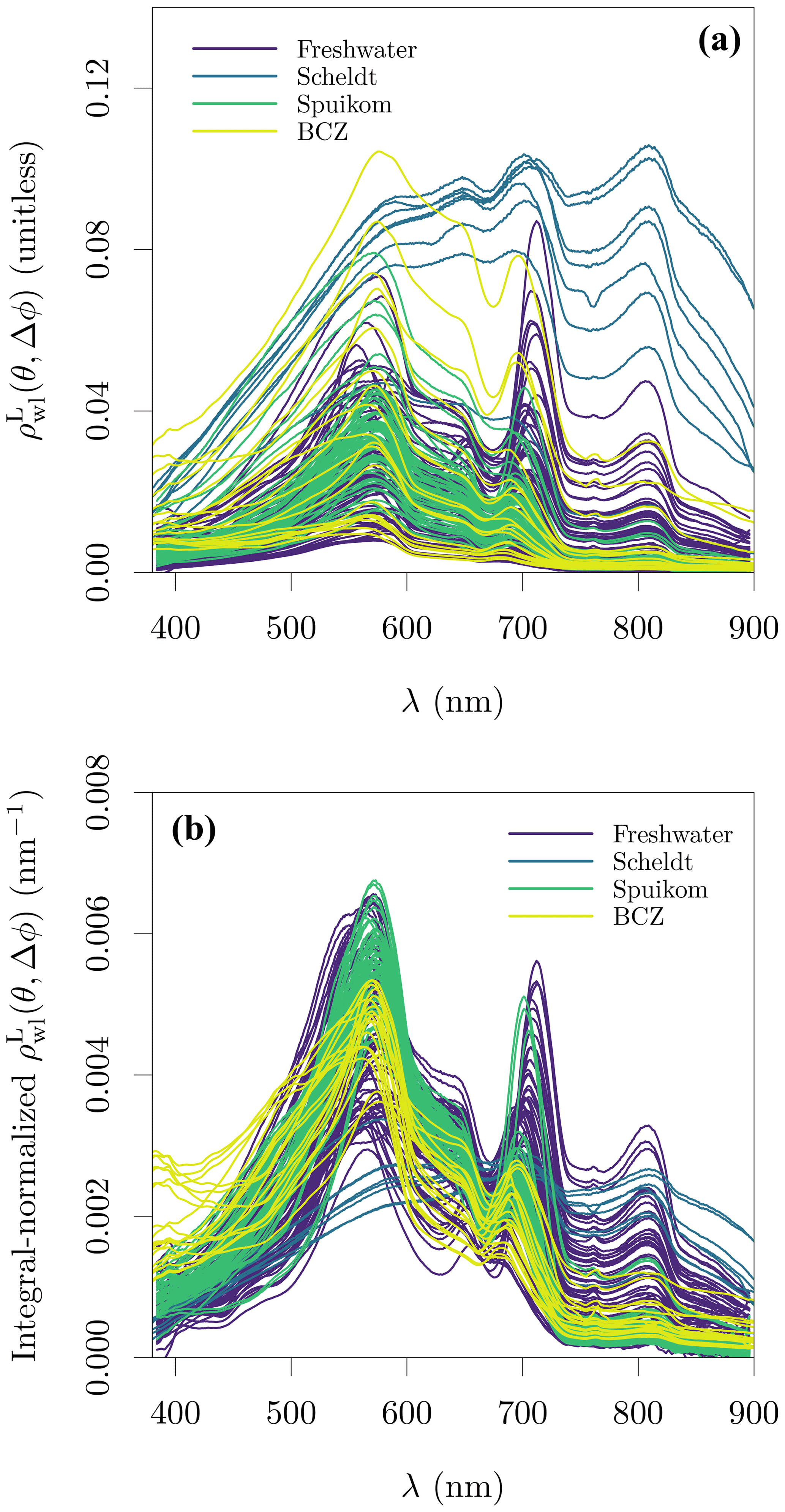
Figure 8Lambert-equivalent water-leaving bi-hemispherical reflectance, , estimated on Belgian water systems. The view geometry is dependent on the measurement approach, being nadir view (θ=0∘) for lakes and the Spuikom, and θ=40∘ Δϕ=135∘ for the Scheldt and the BCZ. (a) Magnitude of and (b) its integral normalisation with respect to wavelength. values measured with the on-water approach presented here were corrected for shadowing.

Figure 9Assessment of data quality by comparing the turbidity estimated from reflectance using the algorithm of Nechad et al. (2010) to the measured turbidity.
For the BCZ campaigns of 2018, reflectance spectroscopy measurements were also made with the above-water approach, using a set of three spectroradiometers (VIS-ARC RAMSES, TriOS) fixed on the bow of the RV Simon Stevin (Castagna et al., 2021). The effective Fresnel reflectance was estimated from wind speed and Lsky according to Ruddick et al. (2006). Further details of processing and quality control are described in Ruddick et al. (2006). The RAMSES instruments have a typical bandwidth of 10 nm FWHM with spectral sampling every ≈ 3 nm. Radiance and irradiance measurements were resampled to a regular 2.5 nm interval before Eq. (8) was applied, and was linearly interpolated to a 1 nm interval to match the other reflectance data. The above-water measurements were not corrected for possible disturbances by the platform in the spectroscopic measurements (Shang et al., 2020) and were not corrected for the non-nadir viewing geometry (Gleason et al., 2012).
The available and are presented in Fig. 8. As expected from the wide range of SPM concentrations, at 810 nm varied over three orders of magnitude, from 0.00036 to 0.10560. Similarly, the large diversity in terms of particle composition (e.g. mineral fraction, taxonomy, pigment) and relative contribution of aΦ translate into a diversity of spectral shapes. A validation of and the shadowing correction for the on-water approach is provided in Fig. 9, by estimating turbidity from following the algorithm proposed by Nechad et al. (2010). The Nechad et al. (2010) algorithm was calibrated with data between ≈ 1 and ≈ 100 g m−3, and the comparison is restricted to that range, covering all systems with the exception of the Scheldt.
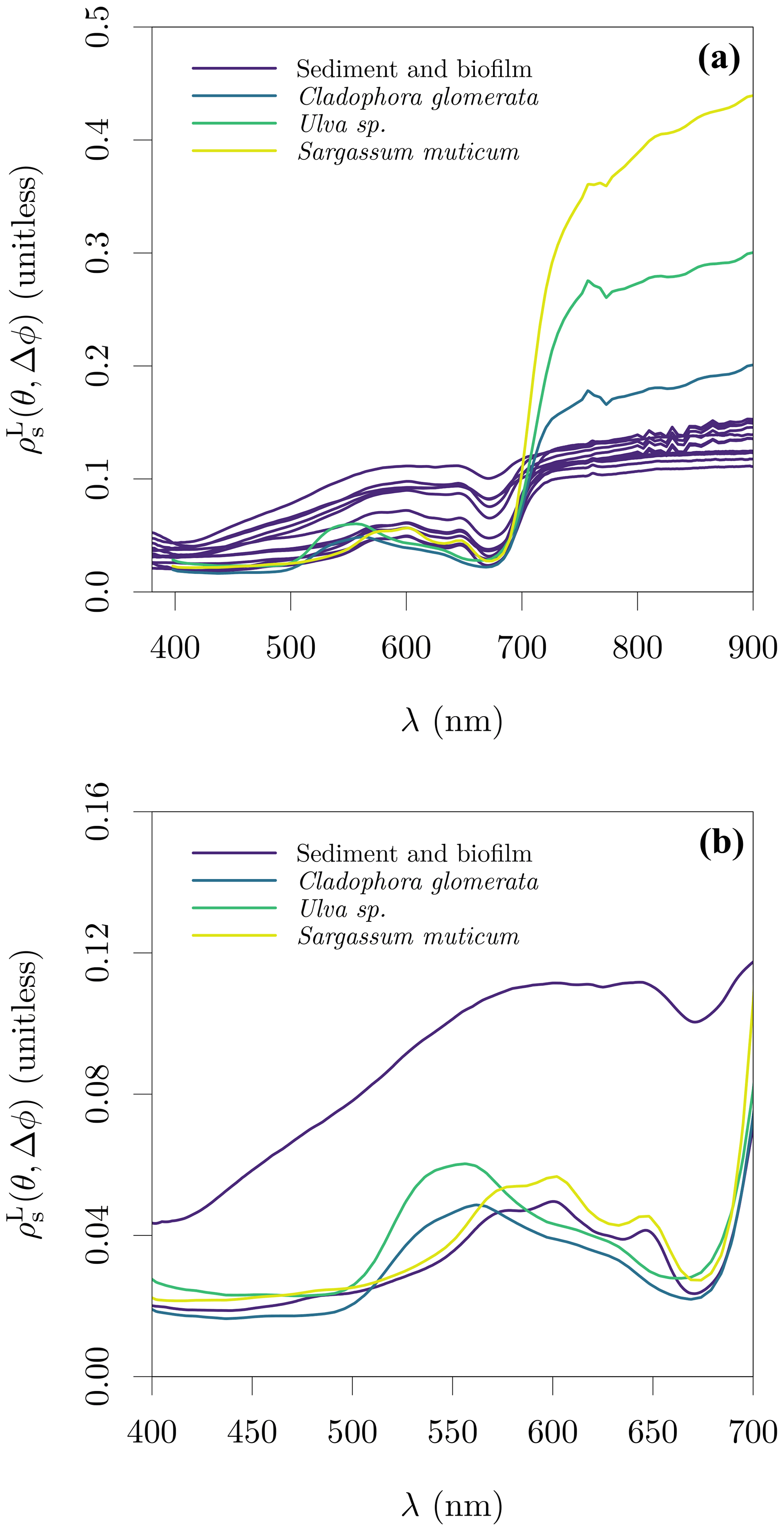
Figure 10Lambert-equivalent substrate bi-hemispherical reflectance, , estimated from samples on the Spuikom. The view geometry was nadir view (θ=0∘, Δϕ undefined) for all measurements. (a) The magnitude of in the visible to NIR spectral range and (b) the magnitude in the visible spectral range. In panel (b), only the sediment samples with the thinnest and thickest biofilm mats are shown, as judged by the reflectance magnitude at 676 nm.
2.4.3 Lambert-equivalent bi-hemispherical reflectance of bottom substrates
Measurements of reflectance spectroscopy of the surface of the sediment cores were made with the portable spectrometer described previously (FieldSpec HH, Analytical Spectral Devices). The PMMA tubes were cut 5 cm above the sediment's surface level and measurements made in nadir view, with 2.5 cm of water above the sediment. Measurements were performed with the on-water approach as described previously, i.e. an extension to the shield of the foreoptics was submerged to 2.5 cm below the water surface. A circular NIST-traceable Munsel card was used as a submerged reference, gently placed over the sediment and receiving the same illumination as the sediment's surface. An example of the measurement setup is shown in Fig. S8 in the Supplement. The bottom depth at the sampled stations varied between 1.3 and 1.93 m, and all but the station SP_43 (1.3 m deep) had the Secchi disc depth above the bottom (average Secchi disc depth of 1.4 m). In July 2018, reflectance spectroscopy measurements were also made of floating biofilm mats that had detached from the bottom of the Spuikom, presumably due to enhanced buoyancy caused by bubbles trapped in the mucilage matrix following several days of high irradiance and heat. Measurements were performed from a boat, without disturbing the floating biofilm mats. A sample taken for microscopy examination revealed an assemblage composed of representatives of the benthic diatom genera Pleurosigma, Gyrosigma, and Navicula (Fig. S9 in the Supplement).
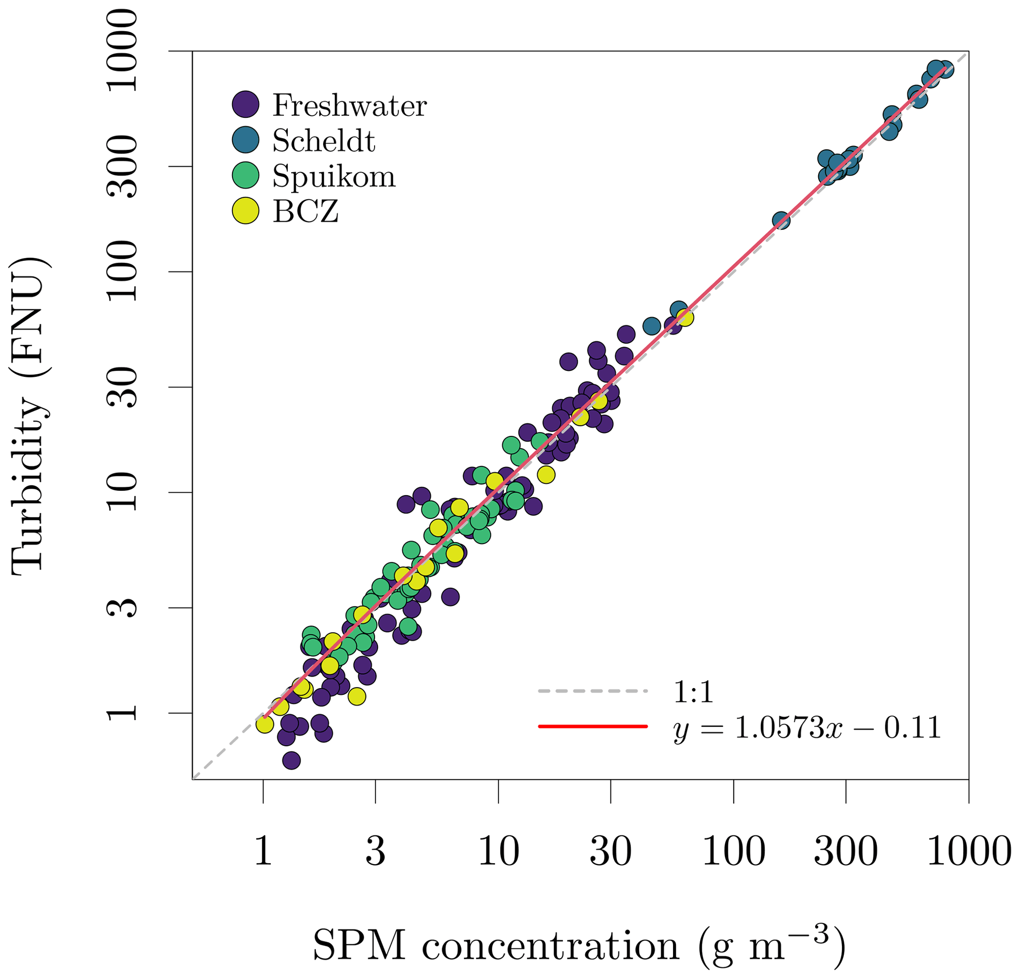
Figure 11Relation between suspended particulate matter (SPM) concentration and turbidity in Belgian water systems.
Reflectance spectroscopy measurements of the most conspicuous macrophyte species occurring in the Spuikom (Cladophora glomerata, Ulva sp., and Sargassum muticum) were performed in air with a hyperspectral camera (SOC710-VP, Surface Optics Corporation). The macrophyte reflectance measurements were made in nadir view with natural illumination. The hyperspectral camera was set up 1 m above the samples, using an f/2.8 aperture following the observation of lower spatial variability in the visible to red-edge spectral region. The 12 % (nominal) reflectivity sintered PTFE plaque was used to estimate Ed and a spectrally flat 5 % reflectivity sheet was used as background. Specimens were folded over a supporting petridish to avoid signal from the background and the reflectance averaged over circular areas to average over the three dimensional structures (Fig. S10 in the Supplement). As the macroalgae were washed free of sediment before measurements, the determined values represent pure end members of substrate reflectance.
The average spectra of macroalgae and the spectra of sediment samples are presented in Fig. 10. The spectra of macroalgae reached values as high as 0.4 in the NIR range, while sediments, independent of biofilm thickness, had an average in the NIR range of ≈ 0.11. In the visible range, the spectral shape of Sargassum muticum seems indistinguishable from the sediments with thickest biofilms, as expected due to similar pigment composition of brown algae and diatoms. The similarity in pigment composition also explains the similarity between the average of healthy specimens of the green algae Ulva sp. and Cladophora glomerata (Kotta et al., 2014).

Figure 12Particle size distribution (PSD) in the Belgian water systems. (a) Retrieved with the LISST-100X and (b) retrieved with the LISST-200X. The continuous particle number concentration PSD was calculated from the volume concentration PSD assuming spherical particles of median diameter in each size bin and normalising by the width of each logarithmically spaced size bin.
2.5 Biogeochemical data
Table 5Summary of measured and derived biogeochemical parameters per water system.
2.5.1 Suspended particulate matter and mineral fraction
Determinations of suspended particulate matter (SPM) concentration (g m−3) were performed gravimetrically, after filtration of the suspensions with pre-treated glass fibre filters (GF/F, Whatman, nominal mesh size of 0.7 µm). For brackish and marine samples, the filters were rinsed with distilled water to remove salt from the filtration area and rim of the filter (Strickland and Parsons, 1968). The filters were then dried overnight at 60 ∘C and cooled to room temperature before mass determinations. The pre-treatment of filters involved combustion for 1 h at 450 ∘C to eliminate organic components, followed by washing to remove loose glass fibres and blank mass determinations. To calculate the mineral fraction (fm) of the SPM, the filters were heated to 500 ∘C for 1 h for thermal oxidation of organic matter and cooled to room temperature before new mass determinations. For some filters, the last mass determinations were lower than the blank mass, indicating a combination of very low mineral fraction and loss of glass fibres during manipulation. Those samples had the mineral fraction set to zero. The observed range of SPM across all systems was 1.02 ± 0.09 to 791.19 ± 0.10 g m−3 and the range of mineral fraction was 0 ± 0.00 to 0.95 ± 0.08. A comparison between SPM and turbidity is presented in Fig. 11.
2.5.2 Particle size distribution
The particle size distribution (PSD) was inverted from the LISST measurements of VSF, using the random-shaped particle VSF kernels provided by the manufacturer. The LISST-100X with random-shaped particle inversion provides the PSD between 1.8 and 381 µm in 32 log-spaced intervals, while the LISST-200X provides the PSD between 1 µm and 500 µm in 36 log-spaced intervals. The LISST software automatically flags measurements with transmittance lower than 30 %. For further details of the measurements with the LISST, see Sect. 2.3.3. Values are provided as volume concentration PSD (cm3 m−3, ppm). The PSDs converted to particle number concentration, using the volume of a sphere with the median diameter of each retrieved bin size range (Buonassissi and Dierssen, 2010), are shown in Fig. 12. Assessing differences in the PSD measured with the two instruments is under further investigation, but beyond the scope of this data report.
2.5.3 Pigment concentration
Pigment mass concentrations were determined using high-performance liquid chromatography (HPLC), following the method of Van Heukelem and Thomas (2001). Cells were broken with sonication and the suspension was cleared by filtration through a 0.22 µm syringe filter. The HPLC apparatus was equipped with a reverse-phase column (Eclipse XDB C8) and detection was performed with spectral absorption (Agilent 1100 series, Diode Array Detector). Pigment standards were acquired from the Danish Hydrographic Institute (DHI) and quantified pigments are listed in Table 6. For the BCZ samples, the measurements are part of the regular marine LifeWatch BE sampling campaigns (Flanders Marine Institute, 2021a) described in Mortelmans et al. (2019). The observed range of total Chl a (Chl a + Chlide a) across all systems was 0.63 to 387.53 mg m−3. Figure 13 presents the distributions of total Chl a per system and the spread of Chl b to total Chl c (Chl c1c2 + Chl c3).
Table 6List of quantified pigments. Names and abbreviations follow Roy et al. (2011). Known co-elutions according to Van Heukelem and Thomas (2001) are described in the table footnotes.
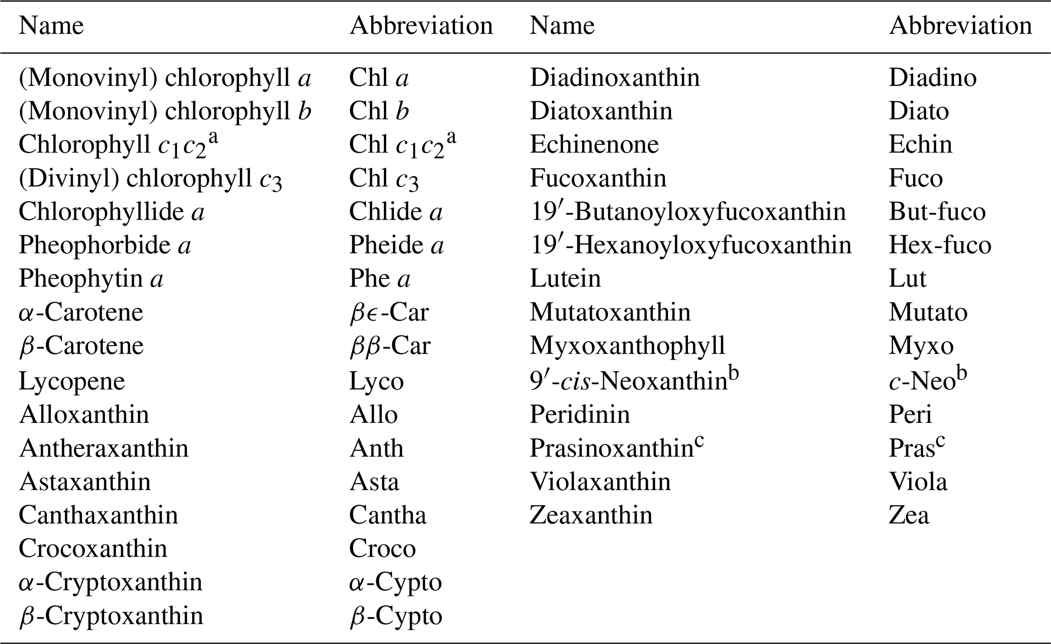
a Chl c1c2 = Chl c1 + Chl c2 + magnesium 2,4-divinylpheoporphyrin a5 monomethyl ester (MgDVP). MgDVP is present in trace concentrations in most algae and cyanobacteria, but is a major component of PRASINO 3A and 3B pigmentation groups (sensu Jeffrey et al., 2011); b c-Neo and 19′-hexanoyloxy-4-ketofucoxanthin (Hex-kfuco) co-elute and are not know to co-occur in the same organism or pigmentation group (sensu Jeffrey et al., 2011); c Pras and micromonol (Microl) co-elute and co-occur in the PRASINO 3B pigmentation group (sensu Jeffrey et al., 2011).
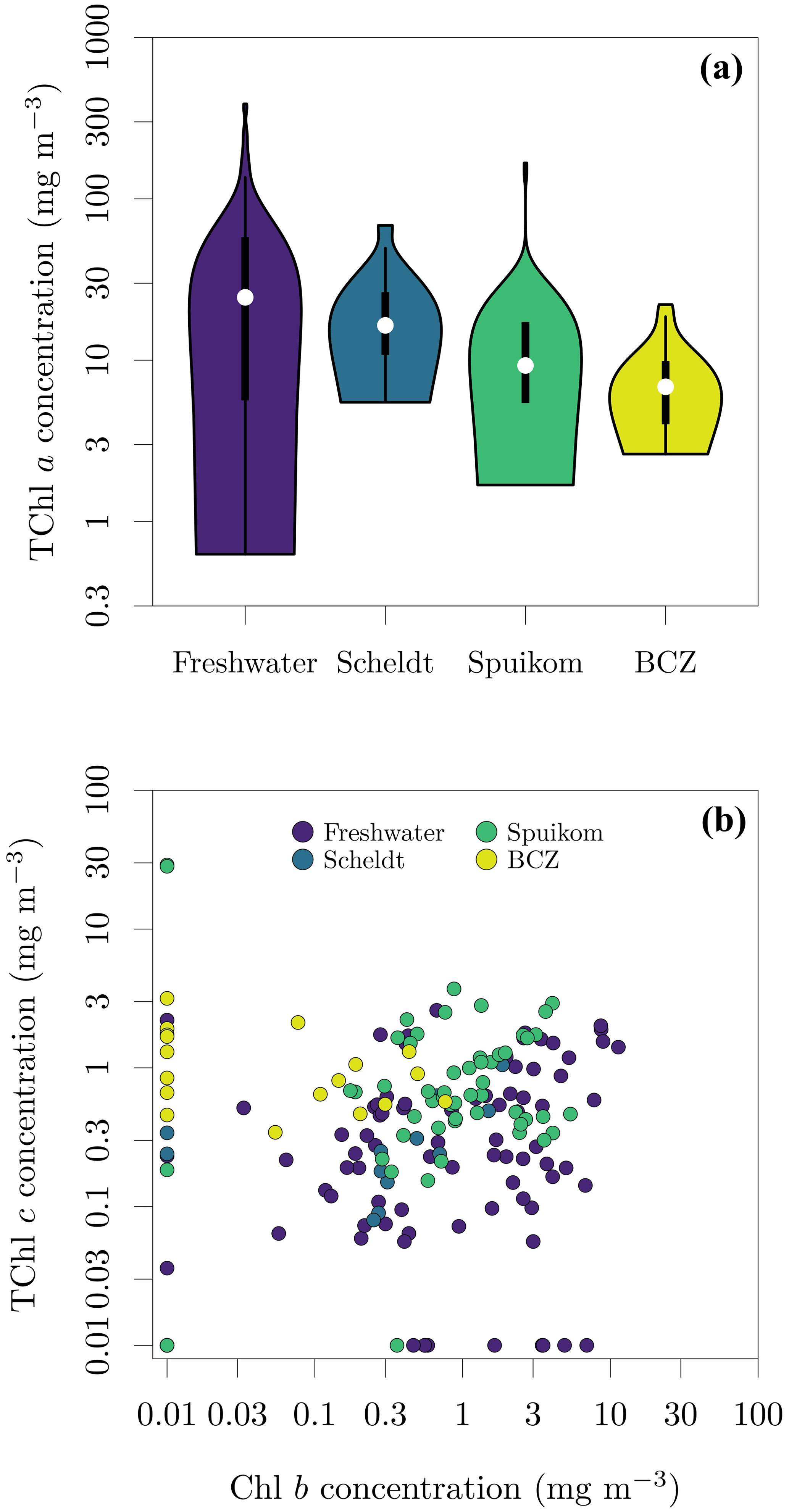
Figure 13Pigment concentrations in Belgian water systems. (a) Total chlorophyll a (TChl a) concentration; and (b) relation between monovinyl chlorophyll b (Chl b) and total chlorophyll c (TChl c) concentrations. TChl a = monovinyl chlorophyll a + chlorophyllide a, TChl c = chlorophyll c1c2 + divinyl chlorophyll c3 (cf. Table 6). A value of 0.01 mg m−3 was added to represent in the log-log plot the samples with concentrations below the detection limit.
2.5.4 DNA metabarcoding
DNA metabarcoding (amplicon sequencing) was performed only for samples from the Spuikom and the BCZ. The molecular analysis was based on replicate filters collected for pigment analysis. DNA extraction was performed with the DNeasy Plant Mini Kit (Qiagen), with polymerase chain reaction (PCR) amplification targeting the variable region 4 (V4) of the nuclear 18S ribosomal RNA gene. The 18S rRNA V4 primers were TAReuk454FWD1 (5' CCAGCASCYGCGGTAATTCC 3') and TAReukREV3 (5' ACTTTCGTTCTTGATYRA 3'; Stoeck et al., 2010). Paired-end (2×300 base pairs) sequencing was performed with the Illumina MiSeq technology (Illumina, San Diego, US) by Genewiz (Leipzig, Germany). The primers were trimmed from the sequenced reads using the FASTX-Toolkit (Gordon and Hannon, 2010). The resulting base-pair sequences were processed with the DADA2 algorithm (Callahan et al., 2016) to resolve amplicon single variants (ASVs). Probable contaminant sequences were removed using negative controls, following the method of Davis et al. (2018). Taxonomic assignment to the ASVs was based on the Protist Ribosomal Reference database (PR2 version 4.12; Guillou et al., 2012). The raw molecular data can be found at the Sequence Read Archive (SRA) of the National Center for Biotechnology Information (NCBI) under accession number PRJNA778668 (https://www.ncbi.nlm.nih.gov/sra/PRJNA778668).
The raw data were further processed to an aggregation level that is relevant for optical monitoring. The assigned taxonomy with PR2 was updated to follow the taxonomy of the World Register of Marine Species (WoRMS Editorial Board, 2021), aggregated to species rank, and filtered to remove non-pigmented organisms. Heterotrophic organisms were filtered at division rank, with the exception of exclusively heterotrophic dinoflagellates, which were filtered at the lowest rank possible based on reference sources (Hasle et al., 1997; WoRMS Editorial Board, 2021). The data were further annotated to indicate (1) the pigmentation group (sensu Jeffrey et al., 2011) of each species based on our pigment ratio database and (2) the toxicity based on the IOC-UNESCO HAB reference list (Moestrup et al., 2021). More than 200 different species from 19 classes of phytoplankton were identified.
2.5.5 Flow imaging microscopy
As part of the regular LifeWatch BE samples in the BCZ, organisms in the range of 55 to 300 µm were counted and identified to the lowest taxonomic unit possible using flow imaging microscopy (FlowCam VS IV, Fluid Imaging Technologies, Inc.; Amadei Martínez et al., 2020; Flanders Marine Institute, 2021b). Fresh water samples were fixed with lugol and stored in the dark until analysis. The images were analysed with the VisualSpreadsheet software (Fluid Imaging Technologies, Inc.) for automatic taxonomic identification. Data were visually inspected to validate the classification. Fixation with lugol results in disaggregation of Phaeocystis globosa colonies and single-cell P. globosa were not detected due to the lower size range of the instrument configuration. In total, 30 different species were detected, the majority of which were diatoms. A comparison of the spatio-temporal pattern of relative abundance of Rhizosolenia spp. cells between amplicon sequencing and FlowCam is shown in Fig. 14.
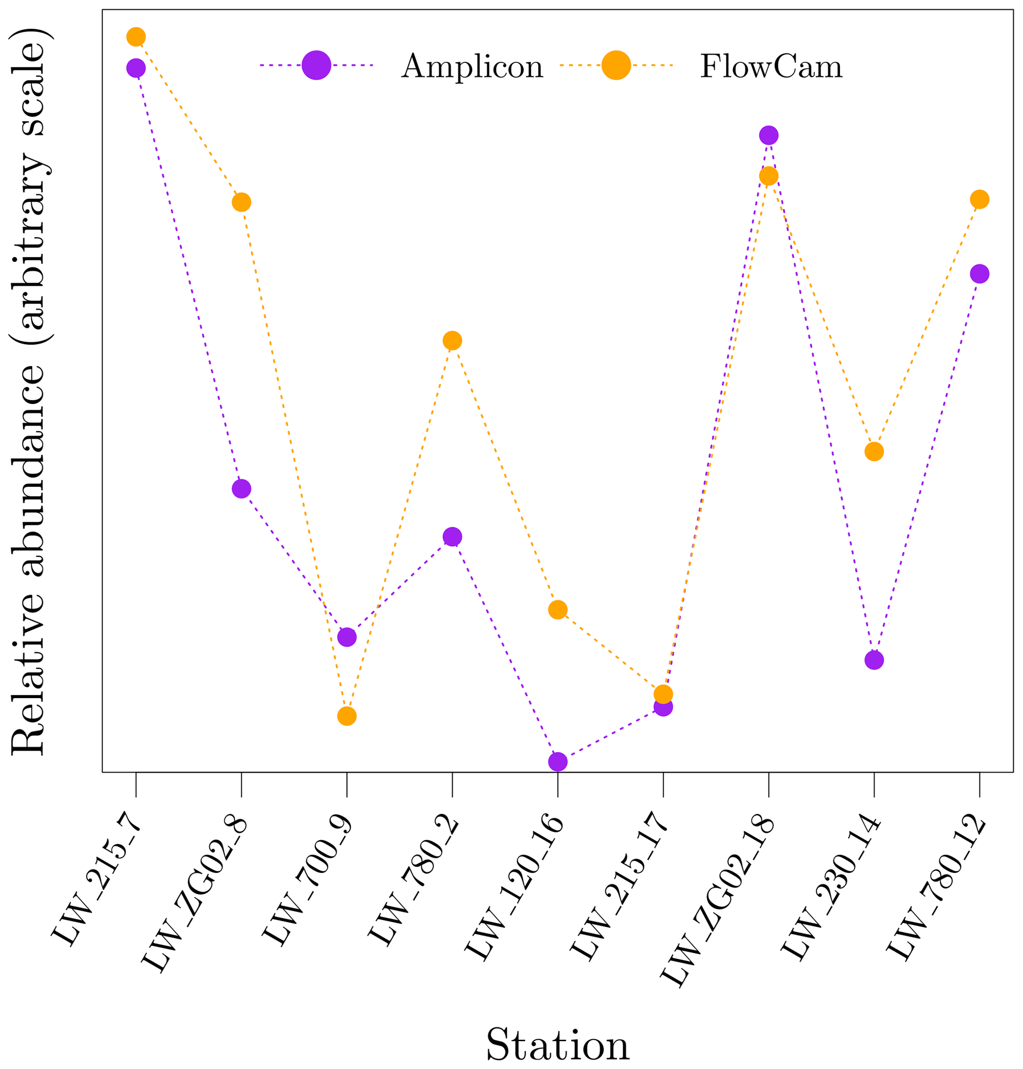
Figure 14Relative abundance of Rhizosolenia spp. cells as estimated by DNA metabarcoding (amplicon sequencing) and microscopy (FlowCam). Data normalised using the counts of common species of diatoms in each dataset.
2.5.6 Bottom cover
For systems in which the bottom can be visualised from the surface, the bottom type was described. Bottom cover was classified based on visual inspection from the surface or from images taken with a submersible camera (Fig. 15). For some stations the bottom cover was classified based on sampling of bottom material. The discrete classes were (1) sediment (potentially with biofilm); (2) shells; (3) Cladophora; (4) Sargassum; (5) brown algae (not specified); and (6) heterogeneous. The last class was used when the bottom was covered by a complex mixture of other classes. This classification is qualitative in the sense that it describes the major composition of the bottom at a given station, but does not provide fractional cover.
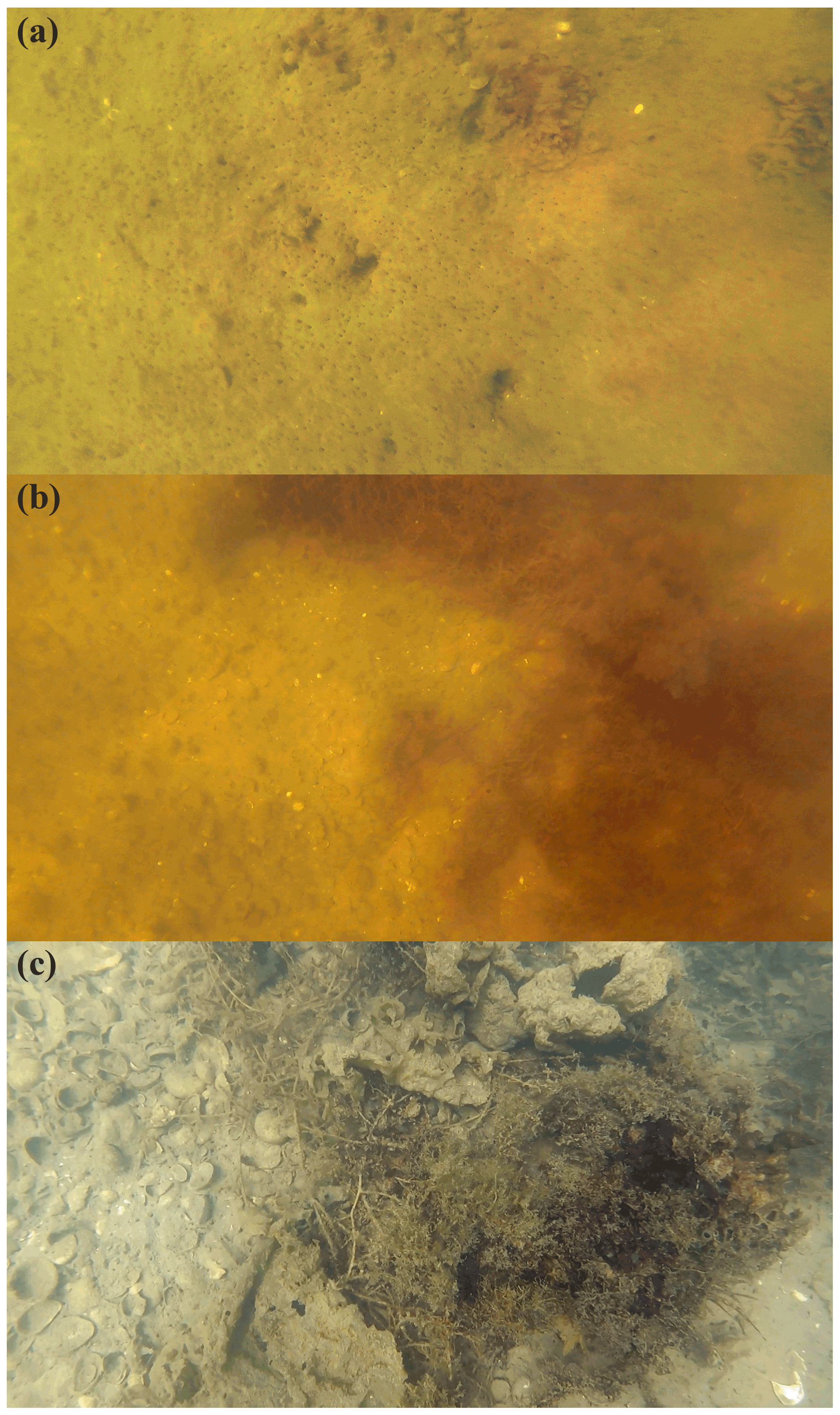
Figure 15Example of bottom-cover classes in the Spuikom. (a) Sediment (with biofilm); (b) sediment, shells, and brown algae; (c) heterogeneous.
2.6 Ancillary parameters
In addition to the optical and biogeochemical parameters, a series of ancillary parameters were also determined: time, position, local depth, sampling platform, sun zenith angle, and visual descriptions of the sky and water system.
For the inland water campaigns, time and the position of each station were recorded from a handheld Global Navigation Satellite System (GNSS) receiver (GPSmap 62s, Garmin), which is enabled to receive corrections from the European Geostationary Navigation Overlay Service (EGNOS). The local depth at the time of sampling was estimated with a handheld single-beam echosounder (Echotest II, Plastino) at the start of each station. The exception was one very shallow station (0.2 m), where a folding ruler was used. For marine stations, position, time, and local depth were taken from the ship's navigation data, acquired with a differential GPS and a mounted single-beam echosounder (JFE 380-25, Japan Radio Co., Ltd.). Sun zenith angles were calculated with the HORIZONS system (Jet Propulsion Laboratory, NASA; https://ssd.jpl.nasa.gov/horizons/, last access: 1 December 2019). All ancillary parameters, with the exception of the sun zenith angle, were combined into a single metadata file.
This study described in detail the first open dataset of paired optical and biogeochemical measurements in a diverse set of water systems located in Belgium. The wide range of observed conditions and the relative scarcity of similar open datasets in inland waters make this a relevant contribution to the community. Potential users of this dataset are encouraged to contact the authors for further inquiries concerning the data and an updated status of studies in development using the dataset.
Although the raw measured IOPs and AOPs are provided, their fitted or corrected versions are recommended for use. For example, the fitted ag removes noise and oscillation in the NIR range due to salinity mismatch between blanks and brackish or marine samples. The fitted ad was found to be the least biased way to remove the absorption signal of NaClO, providing the best estimate of ad and aΦ. The bp, and consequentially cp, corrected to an acceptance angle of 0.018∘ (equivalent to the LISST instruments) provides a more accurate estimate of the scattering and beam attenuation. The dSecchi was corrected for the sun zenith angle, normalising all measurements to the sun in the zenith, and values measured with the on-water method were corrected for platform and instrument shadowing. The results of fitting and corrections were evaluated through consistency checks between different data types and instruments, as presented in the text.
Data are available from Castagna et al. (2022), hosted at PANGAEA under https://doi.org/10.1594/PANGAEA.940240.
The supplement related to this article is available online at: https://doi.org/10.5194/essd-14-2697-2022-supplement.
AC, RD, and ID performed field campaigns in Belgian lakes. AC, HL, KR, MBe, AD, and DD participated on field campaigns in the Spuikom, Scheldt, and BCZ. LAM joined the Sheldt and BCZ campaigns, JM joined BCZ campaigns, and HMD joined Spuikom campaigns. AC performed laboratory measurements of IOPs, field and laboratory measurements of AOP, processing of LISST data, measurements of turbidity, SPM and mineral fraction, classification of the bottom cover, curated the data, and wrote the manuscript. MBe performed reflectance spectroscopy measurements in the BCZ. ID and RD performed HPLC analysis of pigments. MBo and AC performed analysis of DNA metabarcoding. LAM performed flow microscopy counts. HMD, KS, and WV provided infrastructure, planning, and methodological discussion. All authors reviewed the manuscript.
The contact author has declared that neither they nor their co-authors have any competing interests.
Publisher's note: Copernicus Publications remains neutral with regard to jurisdictional claims in published maps and institutional affiliations.
This research was funded by BELSPO Stereo III projects PONDER (SR/00/325), HYPERMAQ (SR/00/335), and PHYTOBEL (SR/02/213). Heidi Dierssen acknowledges funding by NASA Ocean Biology and Biochemistry through the Plankton, Aerosol, Cloud, ocean Ecosystem (PACE) project (NNX15AC32G). We are thankful to the RV Simon Stevin crew for support during LifeWatch BE campaigns, to Darja Belišová, Heidi Tantu, Kathryn Morrissey, Reinhoud de Blok, and Tine Verstraete for help in selected field campaigns, to Sofie D'hondt for the extraction and amplification of the bulk plankton DNA, to Willem Stock for identification of benthic diatoms in the floating biofilms, to Olivier De Clerck for identification of macroalgae, to Koen De Rycker for operating the short corer, to Dieter Vansteenwegen and André Cattrijsse for support during the BCZ and two extended campaigns in the Spuikom, and to the Café Zates for support during the Scheldt campaigns. We are appreciative of all researchers and steering committee members of the PONDER and HYPERMAQ projects for the interesting discussions during development of this research. We appreciate the editor François G. Schmitt and the suggestions provided by Arnold Dekker, Bing Han and an anonymous reviewer. We acknowledge the R Core Team and the authors of the R packages for developing and maintaining the free software used in this research. BCZ data provided as part of the Flemish contribution to the LifeWatch ESFRI by the Flanders Marine Institute (VLIZ).
This research has been supported by the Belgian Federal Science Policy Office (grant nos. SR/00/325, SR/00/335, and SR/02/213) and the Earth Sciences Division (grant no. NNX15AC32G).
This paper was edited by François G. Schmitt and reviewed by Arnold Dekker, Bing Han and one anonymous referee.
Adler, D. and Kelly, S. T.: vioplot: violin plot, https://github.com/TomKellyGenetics/vioplot (last access: 3 June 2022), r package version 0.3.6, 2020. a
Agrawal, Y. C.: The optical volume scattering function: Temporal and vertical variability in the water column off the New Jersey coast, Limnol. Oceanogr., 50, 1787–1794, https://doi.org/10.4319/lo.2005.50.6.1787, 2005. a
Amadei Martínez, L., Mortelmans, J., Dillen, N., Debusschere, E., and Deneudt, K.: LifeWatch observatory data: phytoplankton observations in the Belgian Part of the North Sea, Biodivers. Data J., 8, e57236, https://doi.org/10.3897/BDJ.8.e57236, 2020. a
Astoreca, R., Ruddick, K., Rousseau, V., Mol, B., Parent, J.-Y., and Lancelot, C.: Variability of the inherent and apparent optical properties in a highly turbid coastal area: impact on the calibration of remote sensing algorithms, EARSeL eProceedings, 5, 1–17, 2006. a
Astoreca, R., Rousseau, V., and Lancelot, C.: Coloured dissolved organic matter (CDOM) in Southern North Sea waters: Optical characterization and possible origin, Estuar. Coast. Shelf S., 85, 633–640, https://doi.org/10.1016/j.ecss.2009.10.010, 2009. a
Astoreca, R., Doxaran, D., Ruddick, K., Rousseau, V., and Lancelot, C.: Influence of suspended particle concentration, composition and size on the variability of inherent optical properties of the Southern North Sea, Cont. Shelf Res., 35, 117–128, https://doi.org/10.1016/j.csr.2012.01.007, 2012. a
Binding, C. E., Jerome, J. H., Bukata, R. P., and Booty, W. G.: Spectral absorption properties of dissolved and particulate matter in Lake Erie, Remote Sens. Enviro., 112, 1702–1711, https://doi.org/10.1016/j.rse.2007.08.017, 2008. a
Boss, E., Taylor, L., Gilbert, S., Gundersen, K., Hawley, N., Janzen, C., Johengen, T., Purcell, H., Robertson, C., Schar, D. W. H., Smith, G. J., and Tamburri, M. N.: Comparison of inherent optical properties as a surrogate for particulate matter concentration in coastal waters, Limnol. Oceanogr. Meth., 7, 803–810, https://doi.org/10.4319/lom.2009.7.803, 2009a. a
Boss, E. S., Slade, W. H., Behrenfeld, M. J., and Dall'Olmo, G.: Acceptance angle effects on the beam attenuation in the ocean, Opt. Express, 17, 1535–1550, https://doi.org/10.1364/OE.17.001535, 2009b. a, b
Buonassissi, C. J. and Dierssen, H. M.: A regional comparison of particle size distributions and the power law approximation in oceanic and estuarine surface waters, J. Geophys. Res.-Oceans, 115, C10028, https://doi.org/10.1029/2010JC006256, 2010. a
Cael, B. B. and Boss, E. S.: Simplified model of spectral absorption by non-algal particles and dissolved organic materials in aquatic environments, Opt. Express, 25, 25486, https://doi.org/10.1364/OE.25.025486, 2017. a
Callahan, B. J., McMurdie, P. J., Rosen, M. J., Han, A. W., Johnson, A. J. A., and Holmes, S. P.: DADA2: High-resolution sample inference from Illumina amplicon data, Nature Methods, 13, 581–583, https://doi.org/10.1038/nmeth.3869, 2016. a, b
Castagna, A., Carol Johnson, B., Voss, K. J., Dierssen, H. M., Patrick, H., Germer, T. A., Sabbe, K., and Vyverman, W.: Uncertainty in global downwelling plane irradiance estimates from sintered polytetrafluoroethylene plaque radiance measurements, Appl. Optics, 58, 4497–4511, https://doi.org/10.1364/AO.58.004497, 2019. a, b
Castagna, A., Simis, S. G. H., Dierssen, H., Vanhellemont, Q., Sabbe, K., and Vyverman, W.: Extending Landsat 8: Retrieval of an Orange contra-Band for Inland Water Quality Applications, Remote Sensing, 12, 637, https://doi.org/10.3390/rs12040637, 2020. a
Castagna, A., Dierssen, H., Organelli, E., Bogorad, M., Mortelmans, J., Vyverman, W., and Sabbe, K.: Optical Detection of Harmful Algal Blooms in the Belgian Coastal Zone: A Cautionary Tale of Chlorophyll c3, Front. Mar. Sci., 8, 1892, https://doi.org/10.3389/fmars.2021.770340, 2021. a, b
Castagna, A., Amadei Martínez, L., Bogorad, M., Daveloose, I., Dassevile, R., Dierssen, H. M., Beck, M., Mortelmans, J., Lavigne, H., Dogliotti, A., Doxaran, D., Ruddick, K., Vyverman, W., and Sabbe, K.: Dataset of optical and biogeochemical properties of diverse Belgian inland and coastal waters, PANGAEA [data set], https://doi.org/10.1594/PANGAEA.940240, 2022. a, b
Chase, A., Boss, E. S., Zaneveld, R., Bricaud, A., Claustre, H., Ras, J., Dall'Olmo, G., and Westberry, T. K.: Decomposition of in situ particulate absorption spectra, Methods in Oceanography, 7, 110–124, https://doi.org/10.1016/j.mio.2014.02.002, 2013. a
Davis, N. M., Proctor, D. M., Holmes, S. P., Relman, D. A., and Callahan, B. J.: Simple statistical identification and removal of contaminant sequences in marker-gene and metagenomics data, Microbiome, 6, 226, https://doi.org/10.1186/s40168-018-0605-2, 2018. a, b
Descy, J.-P., Pirlot, S., Verniers, G., Viroux, L., Lara, Y., Wilmotte, A., Vyverman, W., Vanormelingen, P., Van Wichelen, J., Van Gremberghe, I., Triest, L., Peretyatko, A., Everbecq, E., and Codd, G.: B-BLOOMS 2 – Cyanobacterial blooms: toxicity, diversity, modeling and management, Tech. rep., report number D/2011/1191/45, Belgian Science Policy, Brussels, Belgium, 2011. a, b
Desmit, X., Nohe, A., Borges, A. V., Prins, T., De Cauwer, K., Lagring, R., Van der Zande, D., and Sabbe, K.: Changes in chlorophyll concentration and phenology in the North Sea in relation to de-eutrophication and sea surface warming, Limnol. Oceanogr., 65, 828–847, https://doi.org/10.1002/lno.11351, 2020. a
Dierssen, H., Bracher, A., Brando, V., Loisel, H., and Ruddick, K.: Data Needs for Hyperspectral Detection of Algal Diversity Across the Globe, Oceanography, 33, 74–79, https://doi.org/10.5670/oceanog.2020.111, 2020. a
Dogliotti, A. I., Ruddick, K. G., Nechad, B., Doxaran, D., and Knaeps, E.: A single algorithm to retrieve turbidity from remotely-sensed data in all coastal and estuarine waters, Remote Sens. Environ., 156, 157–168, https://doi.org/10.1016/j.rse.2014.09.020, 2015. a
Estapa, M. L., Boss, E., Mayer, L. M., and Roesler, C. S.: Role of iron and organic carbon in mass-specific light absorption by particulate matter from Louisiana coastal waters, Limnol. Oceanogr., 57, 97–112, https://doi.org/10.4319/lo.2012.57.1.0097, 2012. a
Ferrari, G. M. and Tassan, S.: A method using chemical oxidation to remove light absorption by phytoplankton pigments, J. Phycol., 35, 1090–1098, https://doi.org/10.1046/j.1529-8817.1999.3551090.x, 1999. a
Fettweis, M. and Van den Eynde, D.: The mud deposits and the high turbidity in the Belgian–Dutch coastal zone, southern bight of the North Sea, Conti. Shelf Res., 23, 669–691, https://doi.org/10.1016/S0278-4343(03)00027-X, 2003. a, b
Flanders Marine Institute: LifeWatch observatory data: nutrient, pigment, suspended matter and secchi measurements in the Belgian Part of the North Sea, https://doi.org/10.14284/441, 2021a. a
Flanders Marine Institute: LifeWatch observatory data: phytoplankton observations by imaging flow cytometry (FlowCam) in the Belgian Part of the North Sea, https://doi.org/10.14284/527, 2021b. a
Frouin, R. J., Franz, B. A., Ibrahim, A., Knobelspiesse, K., Ahmad, Z., Cairns, B., Chowdhary, J., Dierssen, H. M., Tan, J., Dubovik, O., Huang, X., Davis, A. B., Kalashnikova, O., Thompson, D. R., Remer, L. A., Boss, E., Coddington, O., Deschamps, P.-Y., Gao, B.-C., Gross, L., Hasekamp, O., Omar, A., Pelletier, B., Ramon, D., Steinmetz, F., and Zhai, P.-W.: Atmospheric Correction of Satellite Ocean-Color Imagery During the PACE Era, Front. Earth Sci., 7, 145, https://doi.org/10.3389/feart.2019.00145, 2019. a
Gleason, A. C., Voss, K. J., Gordon, H. R., Twardowski, M., Sullivan, J., Trees, C., Weidemann, A., Berthon, J.-F., Clark, D., and Lee, Z.: Detailed validation of the bidirectional effect in various Case I and Case II waters, Opt. Express, 20, 7630, https://doi.org/10.1364/OE.20.007630, 2012. a
Gordon, A. and Hannon, G.: FASTX-Toolkit, http://hannonlab.cshl.edu/fastx_toolkit/index.html (last access: 3 June 2022), version 0.0.13, 2010. a
Guillou, L., Bachar, D., Audic, S., Bass, D., Berney, C., Bittner, L., Boutte, C., Burgaud, G., de Vargas, C., Decelle, J., del Campo, J., Dolan, J. R., Dunthorn, M., Edvardsen, B., Holzmann, M., Kooistra, W. H., Lara, E., Le Bescot, N., Logares, R., Mahé, F., Massana, R., Montresor, M., Morard, R., Not, F., Pawlowski, J., Probert, I., Sauvadet, A.-L., Siano, R., Stoeck, T., Vaulot, D., Zimmermann, P., and Christen, R.: The Protist Ribosomal Reference database (PR2): a catalog of unicellular eukaryote Small Sub-Unit rRNA sequences with curated taxonomy, Nucl. Acids Res., 41, D597–D604, https://doi.org/10.1093/nar/gks1160, 2012. a
Hasle, G. R., Steidinger, K. A., Syvertsen, E. E., Jansen, K., Jhrondsen, J., and Heimdal, B. R.: Identifying Marine Phytoplankton, Elsevier, San Diego, California, https://doi.org/10.1016/B978-0-12-693018-4.X5000-9, 1997. a
Hoepffner, N. and Sathyendranath, S.: Effect of pigment composition on absorption properties of phytoplankton, Mar. Ecol. Prog. Ser., 73, 11–23, https://doi.org/10.3354/meps073011, 1991. a, b, c
IOCCG: Inherent Optical Property Measurements and Protocols: Absorption Coefficient, vol. 1 of IOCCG Ocean Optics and Biogeochemistry Protocols for Satellite Ocean Colour Sensor Validation, IOCCG, Dartmouth, NS, Canada, https://doi.org/10.25607/OBP-119, 2018. a, b, c, d
ISO 7027:1999: Water quality – Determination of turbidity, Standard, International Organization for Standardization, Geneva, CH, 1999. a
Jeffrey, S. W., Wright, S. W., and Zapata, M.: Microalgal classes and their signature pigments, in: Phytoplankton Pigments: Characterization, Chemotaxonomy, and Applications in Oceanography, edited by: Roy, S., Llewellyn, C. A., Egeland, E. S., and Johnsen, G., Cambridge University Press, Cambridge, UK, chap. 1, 3–77, ISBN 9781107000667, 2011. a, b, c, d
Jonaz, M. and Fournier, G. R.: Light Scattering by Particles in Water: Theoretical and Experimental Foundations, Elsevier, Amsterdam, The Netherlands, https://doi.org/10.1016/B978-0-12-388751-1.X5000-5, 2007. a
Kotta, J., Remm, K., Vahtmäe, E., Kutser, T., and Orav-Kotta, H.: In-air spectral signatures of the Baltic Sea macrophytes and their statistical separability, J. Appl. Remote Sens., 8, 1.–14, https://doi.org/10.1117/1.JRS.8.083634, 2014. a
Latimer, P.: The deconvulation of absorption spectra of green plant materials – Improved corrections for the sieve effect, Photochem. Photobiol., 38, 731–734, https://doi.org/10.1111/j.1751-1097.1983.tb03608.x, 1983. a
Lee, Z., Pahlevan, N., Ahn, Y.-H., Greb, S., and O'Donnell, D.: Robust approach to directly measuring water-leaving radiance in the field, Appl. Optics, 52, 1693–1701, https://doi.org/10.1364/AO.52.001693, 2013. a
Lee, Z., Shang, S., Hu, C., Du, K., Weidemann, A., Hou, W., Lin, J., and Lin, G.: Secchi disk depth: A new theory and mechanistic model for underwater visibility, Remote Sens. Environ., 169, 139–149, https://doi.org/10.1016/j.rse.2015.08.002, 2015. a
Lee, Z., Wei, J., Shang, Z., Garcia, R., Dierssen, H. M., Ishizaka, J., and Castagna, A.: On-Water Radiometry Measurements: Skylight-Blocked Approach and Data Processing (Appendix to IOCCG Protocol Series 2019), Tech. Rep. December, 2019. a
Leymarie, E., Doxaran, D., and Babin, M.: Uncertainties associated to measurements of inherent optical properties in natural waters, Appl. Optics, 49, 5415–5436, https://doi.org/10.1364/AO.49.005415, 2010. a
Max, J.-J. and Chapados, C.: IR spectroscopy of aqueous alkali halide solutions: Pure salt-solvated water spectra and hydration numbers, J. Chem. Phys., 115, 2664–2675, https://doi.org/10.1063/1.1337047, 2001. a, b
Meire, P., Ysebaert, T., Van Damme, S., Van Den Bergh, E., Maris, T., and Struyf, E.: The Scheldt estuary: A description of a changing ecosystem, Hydrobiologia, 540, 1–11, https://doi.org/10.1007/s10750-005-0896-8, 2005. a
Mobley, C. D.: Estimation of the remote-sensing reflectance from above-surface measurements, Appl. Optics, 38, 7442, https://doi.org/10.1364/AO.38.007442, 1999. a
Moestrup, Ø., Akselmann-Cardella, R., Churro, C., Fraga, S., Hoppenrath, M., Iwataki, M., Larsen, J., Lundholm, N., and Zingone, A.: IOC-UNESCO Taxonomic Reference List of Harmful Micro Algae, https://doi.org/10.14284/362, 2021. a
Morel, A. Y. and Bricaud, A.: Theoretical results concerning light absorption in a discrete medium, and application to specific absorption of phytoplankton, Deep-Sea Res. Pt. A, 28, 1375–1393, https://doi.org/10.1016/0198-0149(81)90039-X, 1981. a
Mortelmans, J., Deneudt, K., Cattrijsse, A., Beauchard, O., Daveloose, I., Vyverman, W., Vanaverbeke, J., Timmermans, K., Peene, J., Roose, P., Knockaert, M., Chou, L., Sanders, R., Stinchcombe, M., Kimpe, P., Lammens, S., Theetaert, H., Gkritzalis, T., Hernandez, F., and Mees, J.: Nutrient, pigment, suspended matter and turbidity measurements in the Belgian part of the North Sea, Sci. Data, 22, 22, https://doi.org/10.1038/s41597-019-0032-7, 2019. a, b
Nardelli, S. C. and Twardowski, M. S.: Assessing the link between chlorophyll concentration and absorption line height at 676 nm over a broad range of water types, Opt. Express, 24, A1374, https://doi.org/10.1364/OE.24.0A1374, 2016. a, b
Nechad, B., Ruddick, K. G., and Park, Y.: Calibration and validation of a generic multisensor algorithm for mapping of total suspended matter in turbid waters, Remote Sens. Environ., 114, 854–866, https://doi.org/10.1016/j.rse.2009.11.022, 2010. a, b, c
Pegau, W. S., Zaneveld, J. R. V., Mitchell, B. G., Mueller, J. L., Kahru, M., Wieland, J., and Stramska, M.: Inherent Optical Properties: Instruments, Characterizations, Field Measurements and Data Analysis Protocols, vol. IV, NASA, 2002. a
Quan, X. and Fry, E. S.: Empirical equation for the index of refraction of seawater, Appl. Optics, 34, 3477, https://doi.org/10.1364/AO.34.003477, 1995. a
R Core Team: R: A Language and Environment for Statistical Computing, Version 4.1.1, R Foundation for Statistical Computing, Vienna, Austria, https://www.R-project.org/ (last access: 3 June 2022), 2020. a
Reid, P. C., Lancelot, C., Gieskes, W. W. C., Hagmeier, E., and Weichart, G.: Phytoplankton of the North Sea and its dynamics: A review, Neth. J. Sea Res., 26, 295–331, https://doi.org/10.1016/0077-7579(90)90094-W, 1990. a
Roesler, C. S. and Barnard, A. H.: Optical proxy for phytoplankton biomass in the absence of photophysiology: Rethinking the absorption line height, Methods in Oceanography, 7, 79–94, https://doi.org/10.1016/j.mio.2013.12.003, 2013. a, b
Roesler, C. S. and Boss, E. S.: Spectral beam attenuation coefficient retrieved from ocean color inversion, Geophys. Res. Lett., 30, 1468, https://doi.org/10.1029/2002GL016185, 2003. a
Röttgers, R., Dupouy, C., Taylor, B. B., Bracher, A., and Woźniak, S. B.: Mass-specific light absorption coefficients of natural aquatic particles in the near-infrared spectral region, Limnol. Oceanogr., 59, 1449–1460, https://doi.org/10.4319/lo.2014.59.5.1449, 2014a. a
Röttgers, R., McKee, D., and Utschig, C.: Temperature and salinity correction coefficients for light absorption by water in the visible to infrared spectral region, Opt. Express, 22, 25093, https://doi.org/10.1364/OE.22.025093, 2014b. a, b
Roy, S., Llewellyn, C. A., Egeland, E. S., and Johnsen, G., eds.: Phytoplankton Pigments: Characterization, Chemotaxonomy, and Applications in Oceanography, Cambridge University Press, Cambridge, UK, ISBN 9781107000667, 2011. a
Ruddick, K. G., Cauwer, V. D., Park, Y.-J., and Moore, G.: Seaborne measurements of near infrared water-leaving reflectance : The similarity spectrum for turbid waters, Limnol. Oceanogr., 51, 1167–1179, https://doi.org/10.4319/lo.2006.51.2.1167, 2006. a, b
Ruddick, K. G., Voss, K. J., Banks, A., Boss, E., Castagna, A., Frouin, R., Hieronymi, M., Jamet, C., Johnson, B., Kuusk, J., Lee, Z., Ondrusek, M., Vabson, V., and Vendt, R.: A review of protocols for Fiducial Reference Measurements of downwelling irradiance for the validation of satellite remote sensing data over water, Remote Sensing, 11, 1742, https://doi.org/10.3390/rs11151742, 2019a. a, b
Ruddick, K. G., Voss, K. J., Banks, A. C., Boss, E. S., Castagna, A., Frouin, R., Hieronymi, M., Jamet, C., Johnson, B. C., Kuusk, J., Lee, Z., Ondrusek, M., Vabson, V., and Vendt, R.: A Review of Protocols for Fiducial Reference Measurements of Downwelling Irradiance for the Validation of Satellite Remote Sensing Data over Water, Remote Sensing, 11, 1742, https://doi.org/10.3390/rs11151742, 2019b. a, b
Shang, Z., Lee, Z., Wei, J., and Lin, G.: Impact of ship on radiometric measurements in the field: a reappraisal via Monte Carlo simulations, Opt. Express, 28, 1439, https://doi.org/10.1364/OE.28.001439, 2020. a
Stoeck, T., Bass, D., Nebel, M., Christen, R., Jones, M. D., Breiner, H. W., and Richards, T. A.: Multiple marker parallel tag environmental DNA sequencing reveals a highly complex eukaryotic community in marine anoxic water, Mol. Ecol., 19, 21–31, https://doi.org/10.1111/j.1365-294X.2009.04480.x, 2010. a
Stramski, D., Reynolds, R. A., Kaczmarek, S., Uitz, J., and Zheng, G.: Correction of pathlength amplification in the filter-pad technique for measurements of particulate absorption coefficient in the visible spectral region, Appl. Optics, 54, 6763, https://doi.org/10.1364/AO.54.006763, 2015. a, b
Strickland, J. D. H. and Parsons, T. R.: A Practical Handbook of Seawater Analys, Fisheries Research Board of Canada, Ottawa, Canada, 1968. a
Twardowski, M. S., Boss, E., Sullivan, J. M., and Donaghay, P. L.: Modeling the spectral shape of absorption by chromophoric dissolved organic matter, Mar. Chem., 89, 69–88, https://doi.org/10.1016/j.marchem.2004.02.008, 2004. a
van Beusekom, J. and Diel-Christiansen, S.: A synthesis of phyto and zooplankton dynamics in the North Sea environment, Tech. rep., 146 pp., ISBN 1 85850 028 1, 1994. a
Van Heukelem, L. and Thomas, C. S.: Computer-assisted high-performance liquid chromatography method development with applications to the isolation and analysis of phytoplankton pigments, J. Chromatogr. A, 910, 31–49, https://doi.org/10.1016/S0378-4347(00)00603-4, 2001. a, b
Venables, W. N. and Ripley, B. D.: Modern Applied Statistics with S, Springer, New York, 4th Edn., ISBN 0-387-95457-0, 2002. a, b
Verschuur, G. L.: Transparency Measurements in Garner Lake, Tennessee: The Relationship between Secchi Depth and Solar Altitude and a Suggestion for Normalization of Secchi Depth Data, Lake Reserv. Manage., 13, 142–153, https://doi.org/10.1080/07438149709354305, 1997. a
WoRMS Editorial Board: World Register of Marine Species (WoRMS), https://doi.org/10.14284/170, 2021. a, b
Zaneveld, J. R. V. and Kitchen, J. C.: The variation in the inherent optical properties of phytoplankton near an absorption peak as determined by various models of cell structure, J. Geophys. Res., 100, 13309, https://doi.org/10.1029/95JC00451, 1995. a