the Creative Commons Attribution 4.0 License.
the Creative Commons Attribution 4.0 License.
 | 25 May 2022
HydroSat: geometric quantities of the global water cycle from geodetic satellites
Mohammad J. Tourian
Omid Elmi
Yasin Shafaghi
Sajedeh Behnia
Peyman Saemian
Ron Schlesinger
Nico Sneeuw
Against the backdrop of global change, in terms of both climate and demography, there is a pressing need for monitoring of the global water cycle. The publicly available global database is very limited in its spatial and temporal coverage worldwide. Moreover, the acquisition of in situ data and their delivery to the database have been in decline since the late 1970s, be it for economical or political reasons. Given the insufficient monitoring from in situ gauge networks, and with no outlook for improvement, spaceborne approaches have been under investigation for some years now. Satellite-based Earth observation with its global coverage and homogeneous accuracy has been demonstrated to be a potential alternative to in situ measurements. This paper presents HydroSat as a database containing geometric quantities of the global water cycle from geodetic satellites. HydroSat provides time series and their uncertainty in water level from satellite altimetry, surface water extent from satellite imagery, terrestrial water storage anomaly represented in equivalent water height from satellite gravimetry, lake and reservoir water volume anomaly from a combination of satellite altimetry and imagery, and river discharge from either satellite altimetry or imagery. The spatial and temporal coverage of these datasets varies and depends on the availability of geodetic satellites. These products, which are complementary to existing products, can contribute to our understanding of the global water cycle within the Earth system in several ways. They can be incorporated for hydrological modeling, they can be complementary to current and future spaceborne observations, and they can define indicators of the past and future state of the global freshwater system. HydroSat is publicly available through http://hydrosat.gis.uni-stuttgart.de (last access: 18 May 2022). Moreover, a snapshot of all the data (taken in April 2021) is available in GFZ Data Services at https://doi.org/10.5880/fidgeo.2021.017 (Tourian et al., 2021).
- Article
(11623 KB) - Full-text XML
-
Supplement
(3399 KB) - BibTeX
- EndNote


To understand the global hydrological cycle and the Earth system in general, measurements are needed to estimate storages and fluxes on a spatial scale from local to continental and on a temporal scale sufficient to resolve even diurnal variations (Lettenmaier, 2006). However, current knowledge of spatial and temporal dynamics of water storage and fluxes on landmasses is limited (Alsdorf and Lettenmaier, 2003). The water surface elevation variation and bathymetry of rivers and lakes are not sufficiently known. The depth of soil moisture is not known on a global scale. Rain gauge measurements are spatially not dense enough to represent the input to the hydrological cycle. The number of discharge gauge stations that contribute to the global database has been declining steadily over the past decades. In fact, by today's knowledge, storage, fluxes and their changes over time cannot be quantified properly. So they still remain our known unknowns on a global scale (Famiglietti, 2012).
Given the abovementioned limitations, estimates from traditional in situ measurements are subject to large uncertainty (Alsdorf and Lettenmaier, 2003; Strassberg et al., 2007; Yeh et al., 2006; Rodell et al., 2006; Riegger et al., 2012). In the past, simple water balance analyses were used to assess spatial patterns of precipitation and evapotranspiration and to produce globally averaged fluxes. The average fluxes were estimated simply as the difference in precipitation minus evapotranspiration, assuming that long-term change in net water storage is negligible (Rodell et al., 2015; Lvovitch, 1973; Berner and Berner, 2012). With the emergence of land surface representations in climate models (e.g., Dickinson, 1984) and large-scale hydrological models (e.g., Vörösmarty et al., 2000), the limited ground-based observations were augmented by model outputs, leading to a finer representation of water cycle on landmasses. The problem, however, is that the model outputs themselves should usually be calibrated or constrained by observations (Rodell et al., 2015).
Spaceborne geodetic sensors, designed for a variety of purposes, have established themselves as valuable tools for oceanographic, cryospheric and also hydrological applications (Alsdorf et al., 2007). Satellite altimetry, originally aiming at oceanography and geodesy, has demonstrated its potential as virtual lake and river gauges (Alsdorf et al., 2007; Papa et al., 2010a; Berry et al., 2005). The exciting possibility of surface water extent monitoring using satellite imagery (optical and synthetic aperture radar, SAR) raises hopes of better capturing surface water variability and providing a realistic overview of hydrological behavior at the basin scale. Since 2002 the satellite mission Gravity Recovery And Climate Experiment (GRACE) has been providing a fundamentally new remote sensing tool for a wide spectrum of Earth science applications (Tapley et al., 2004). GRACE is able to monitor changes in the ocean and the global hydrological cycle through measuring changes in the Earth's gravitational field from space.
The aforementioned missions promote novel approaches in oceanography, geophysics, hydrology and hydro-meteorology. Among these sciences, as stated above, there is an urgent need for more observational data, particularly in hydrology. This necessity arises from the abovementioned limited knowledge of the spatial and temporal dynamics of the freshwater variations and fluxes (Sneeuw et al., 2014). Given such a pressing need, spaceborne geodetic sensors, with their global coverage and homogeneous accuracy, are viable choices over in situ measurements. It should be noted, however, that despite being the only source of information in data-poor regions, satellites do not yet provide the desired spatio-temporal resolution. The spatio-temporal resolution of spaceborne sensors is defined by their orbital characteristics and their measurement concept. Satellite altimetry missions are typically placed in repeat orbits with a given number of revolutions within a certain number of days, e.g., 35 d for ENVISAT, 10 d for Jason series and 27 d for Sentinel series (Fu and Cazenave, 2001). GRACE can provide meaningful signals at its best spatial resolution on the monthly timescale. The spatio-temporal resolution problem is not as pronounced for optical and SAR satellite imaging missions because they provide images with a relatively high spatial resolution (about 250 m for MODIS and 30 m for Landsat) at an acceptable temporal resolution. However, cloud cover is a limiting factor in using the optical images for generating a dense time series of surface water area.
Space-based water cycle monitoring is entering a new era in view of the wealth of present and future missions. Satellite altimetry has already been put on an operational basis by the Sentinel-3 satellites of the European Copernicus program. At the same time, research satellites such as CryoSat-2, SARAL/AltiKa and Jason-3 remain in orbit and provide complementary space–time measurements. On the other hand, MODIS sensors on NASA's Terra and Aqua satellites have been acquiring medium-resolution satellite images daily since 2000. In addition to the MODIS images, high-resolution optical and SAR satellite images are available from Landsat 8 and Sentinel 1 and 2. Moreover, the planned SWOT (Surface Water and Ocean Topography) mission, due for launch in 2022, will represent a paradigm change in monitoring surface water, providing a 2-D swath as opposed to conventional 1-D profiling. SWOT aims to monitor surface water elevation, extent, slope and also river discharge for all rivers wider than 100 m (Biancamaria et al., 2016). In addition, GRACE Follow-On was launched in 2018 to ensure continuity of the GRACE mission after its successful 15-year monitoring of water storage variation. The current constellation addresses many existing limitations and opens a significant area of investigations into the operational use of satellites for hydrological purposes.
Inspired by the increasing need to monitor the global hydrological cycle and by the potential offered by the existing constellation, attempts have been made to monitor hydrological cycle variables using geodetic satellites. The Hydroweb (http://hydroweb.theia-land.fr, last access: 18 May 2022) initiated and monitored by LEGOS, the Database of Hydrological Time Series of Inland Waters (DAHITI) developed by the German Geodetic Research Institute at the Technical University of Munich (DGFI-TUM) (Schwatke et al., 2015a), and the Global Reservoirs and Lakes Monitor (G-REALM) (https://ipad.fas.usda.gov/cropexplorer/global_reservoir, last access: 18 May 2022) are some examples of such attempts. With the same motivation, the HydroSat database was initiated in 2016. HydroSat hosts geometric quantities of the global water cycle from geodetic satellites: (1) surface water extent of lakes and rivers; (2) water level of inland water bodies; (3) water storage anomaly of hydrological basins, lakes and reservoirs; and (4) river discharge for large and small rivers. This is a unique set of products for understanding global water cycle as it contains key elements of water cycle for many ungauged basins around the world. These quantities, which complement existing databases, can contribute to the understanding of the global water cycle by incorporating them into hydrological models, serving as the basis for indicators of the past and future state of the global freshwater system to assess risks under global warming and support decision-making and also complementing current and future spaceborne observations. Moreover, they can effectively be used as potential prior information for future mission products that rely on prior hydrological data for their monitoring concepts, such as the SWOT mission. HydroSat products are the results of research studies and projects on the application of spaceborne geodetic sensors for hydrology conducted at the Institute of Geodesy (GIS), University of Stuttgart. This paper describes HydroSat data products with a detailed explanation of the algorithm behind them: water level time series from satellite altimetry in Sect. 2; river width estimation from satellite imagery in Sect. 3; water storage anomaly for hydrological river basins, lakes and reservoirs in Sect. 4; and, finally, river discharge estimation from satellite altimetry and imagery in Sect. 5. For each data product, some representative examples are given to support the product description.
In the last 3 decades, satellite altimetry has been used as a monitoring tool for inland water surfaces and the hydrological cycle. In particular, monitoring water level of large rivers and lakes has been the goal of research since the launch of the TOPEX/Poseidon and Envisat missions (Table S1) (Birkett, 1995; Crétaux et al., 2011). The use of satellite altimetry for inland water monitoring has been facilitated by the advent of two different developments: (1) open-loop tracking command (OLTC) (used in missions with gray background in Table S1) and (2) operation in synthetic aperture radar (SAR) mode (implemented in missions with bolded text in Table S1).
Inspired by recent developments, and the SWOT mission in view, the development of repositories and services to provide inland water level time series to supply data for Earth system understanding, hydrological cycle monitoring and hydraulic studies is becoming more important than ever. Table 1 lists currently available websites or repositories for providing water level time series of inland water bodies.
Schwatke et al. (2015a)Coss et al. (2020)Markert et al. (2019)Table 1Providers of water level time series from satellite altimetry.
* Last access: 18 May 2022
Hydroweb was the first website providing altimetric water level time series. The website, now hosted on THEIA, is a CNES project, which was initiated and monitored by LEGOS in 2003 based on all existing and past altimetry missions, from TOPEX/Poseidon until Sentinel-3B. A substantial portion of water level time series of lakes and rivers are provided in near-real time (NRT). CNES, LEGOS and CLS have further extended their monitoring services under agreements with Copernicus. As a result, they provide water level time series of 94 selected lakes within the context of the Copernicus Climate Change Service, the so-called C3S LWL. They further provide historical and NRT water level time series of several lakes and rivers through the VITO Earth Observation portal. In 2009, in a cooperation of ESA and De Montfort University, the River & Lake website became available. On this website, which is no longer maintained, global NRT products were available. Later in 2013, the Database for HydrologIcal Time Series of Inland waters (DAHITI) was developed by the Deutsches Geodätisches Forschungsinstitut at the Technical University Munich (DGFI-TUM) to provide water level time series of inland waters (Schwatke et al., 2015a). DAHITI provides a variety of hydrological information on lakes, reservoirs, rivers and wetlands derived from different satellite missions. Since 2017, the Global Reservoirs and Lakes Monitor (G-REALM) has provided time series of water level variations for some of the world's largest lakes and reservoirs. Unlike G-REALM, the Global River Radar Altimeter Time Series (GRRATS) focuses on rivers and provides water level time series over 39 rivers spanning the time period 2002–2016 using Envisat series and Jason series (Coss et al., 2020). Within a rather unprecedented framework, the open-source web application AlteEx allows for exploration of altimetry datasets and generation of water level time series on the fly. AltEx is supported by the US Agency for International Development (USAID) and NASA (Markert et al., 2019; Okeowo et al., 2017).
2.1 HydroSat products for water level
In HydroSat, water level time series are provided in two modes – standard rate (SR) and high rate (HR):
-
standard-rate water level time series from satellite altimetry
-
high-rate altimetric water level over lakes and reservoirs
-
high-rate altimetric water level over lakes and reservoirs
-
high-rate altimetric water level over rivers.
-
A SR water level time series is the basic altimetry product of HydroSat with a temporal resolution given by the repeat period of the altimetry (e.g., 35 d for Envisat). It is the input to algorithms which provide HR water level time series over lakes, reservoirs and rivers. The HR products come with an improved temporal resolution relying on multi-mission altimetry for both lakes and rivers. These products are available over a multitude of lakes and rivers around the world. As an example of SR time series, Fig. 1 shows a representative collection of SR water level time series over Lake Bankim in Cameroon and the Mississippi River in the US, the São Francisco River in Brazil, the Karun in Iran, the Yangtze River in China and the Irrawaddy River in Myanmar. One shall notice that AltEx, C3S LWL and VITO water level are excluded from this comparison. In the case of AltEx, any comparison would have been subjective as the quality of the water level time series is dependent on the geometric choice of a virtual station by the user. As for the C3S LWL and VITO Water Level, we have observed no difference between these time series with those from Hydroweb (the same argument holds for objects shown in Sect. 2.2.3). For the São Francisco (Fig. 1c) and Mississippi (Fig. 1f) rivers, the altimetric heights agree with the in situ measurements with correlation coefficients of 0.99 and 0.97, respectively. In the case of the Karun river (Fig. 1a), the correlation falls off to 0.85, which is satisfactory given the 250 m crossing width, mountainous topography and high seasonality of its semiarid climate. The SR water level time series are well representative of water level dynamics, an example being the case of the Irrawaddy River (Fig. 1d) showing the high rank correlation of 0.91 with in situ discharge measurements. The results over the Yangtze River (Fig. 1e) and Lake Bankim (Fig. 1b) agree well with DAHITI, Hydroweb and G-REALM. Over these water bodies – like many other water bodies around the world – no in situ measurements are publicly available, highlighting the critical contribution of spaceborne measurements and the existing repositories.
Figure 2 shows examples of HR water level time series over a selection of five lakes and reservoirs presenting different behaviors. Lake water level time series provided by HydroSat and other databases (DAHITI, Hydroweb and G-REALM) are in acceptable agreement with in situ measurements; however some differences are noticeable. Over Lake Erie, for instance, HydroSat better captures measurements at the tails of the water level distribution, meaning that the actual fluctuations in lake level are better presented. This is due to the fact that besides outlier rejection, as described in Sect. 2.2.1, no further smoothing is applied. The HR water level time series of Lake Urmia signals yet another difference. All altimetric time series seem to have captured the long-term depletion of the lake level, followed by the recent and ongoing restoration period (Saemian et al., 2020). The majority, however, overestimate the lake level between late 2010 and early 2019. The altimetric measurements during this period are mainly from Jason-2 and Jason-3 missions. The satellite's ground track happens to cross the shallow southeast of the lake. During this 9-year low-water period, the altimeters have measured the range to the salt pan that remains in the southern part after the lake desiccation. Excluding such a measurement without incorporating auxiliary sources of data is rather impossible. HydroSat can deal with this issue within the inter-satellite bias estimation (Fig. S2) by taking the surface area into account. Any SR water level time series that exhibits inconsistency with an expected behavior fails to contribute to the HR lake water level time series.
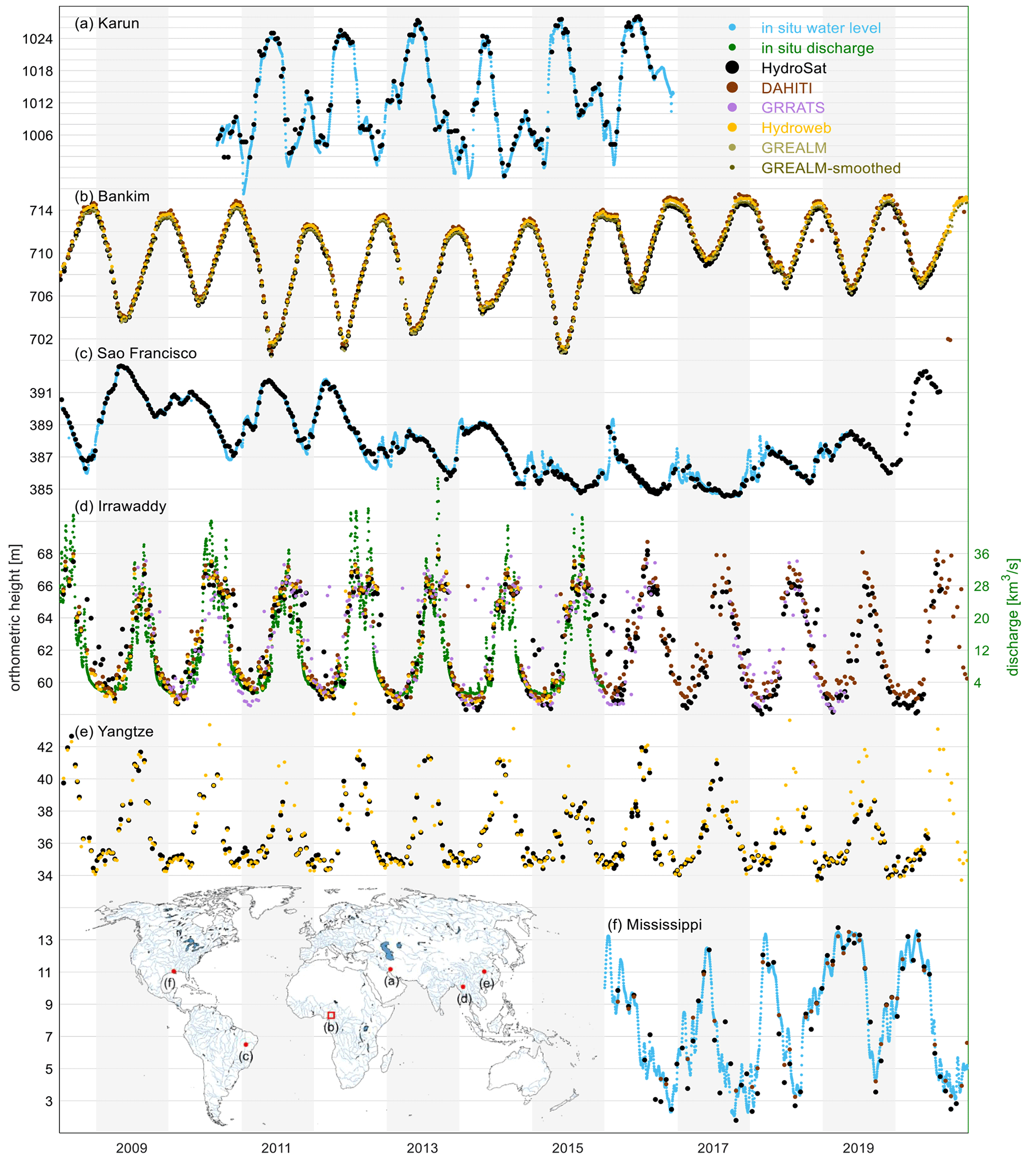
Figure 1Standard-rate altimetric water level time series over the Karun river (Iran) from Jason-2, Lake Bankim (Cameroon) from Jason-2 and Jason-3, the São Francisco River (Brazil) from Jason-2 and Jason-3, the Irrawaddy River (Myanmar) from Jason-2 and Jason-3, the Yangtze River (China) from Jason-2 and Jason-3, and the Mississippi River (US) from Sentinel-3A.
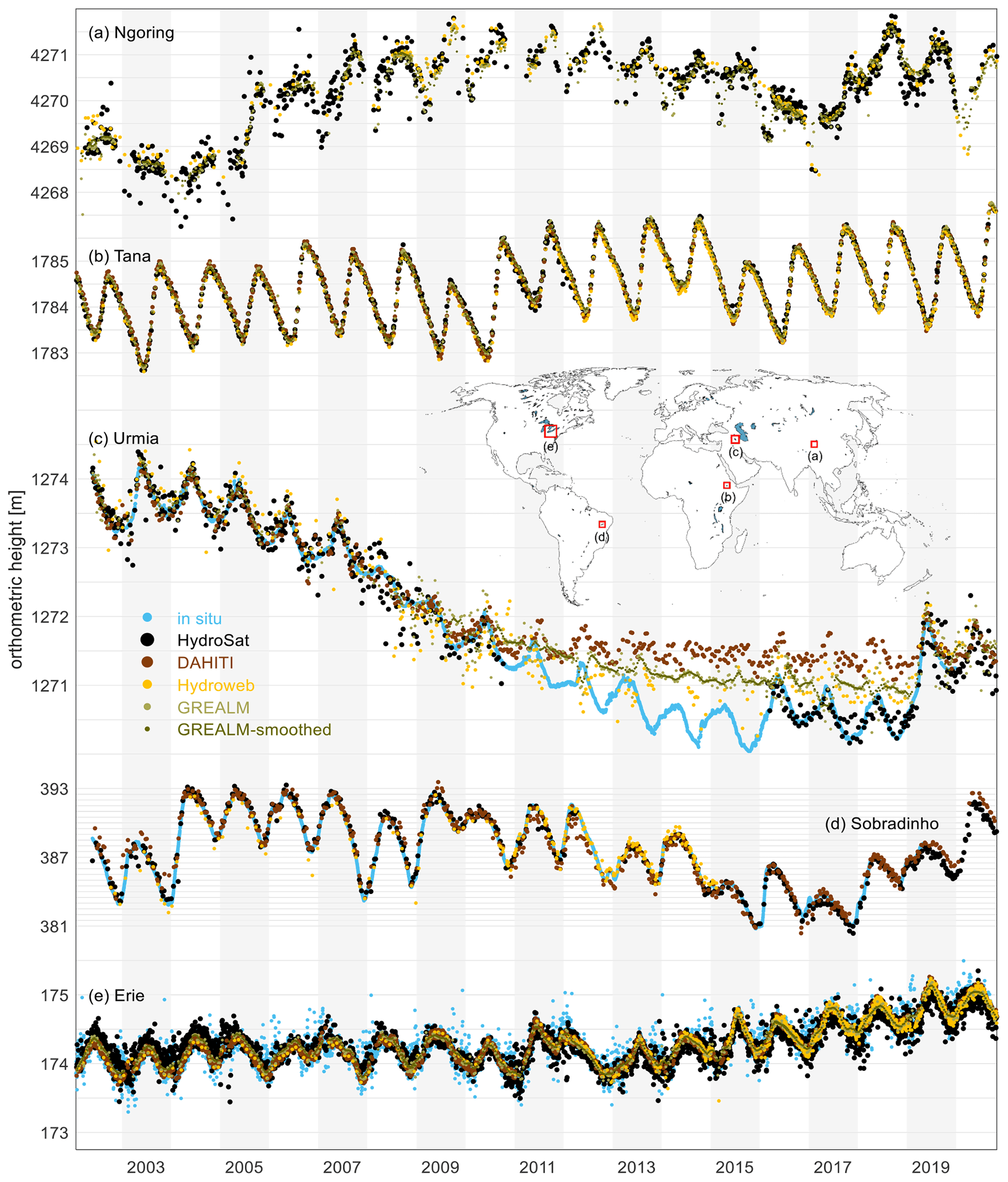
Figure 2High-rate altimetric water level time series over lakes Ngoring in China (610 km2) from Envisat, SARAL/AltiKa, Jason-1, Jason-2, Jason-3 and Sentinel-3A; Tana in Ethiopia (2156 km2) from Envisat, SARAL/AltiKa, Jason-1, Jason-2, Jason-3, Sentinel-3A and Sentinel-3B; Urmia in Iran (5200 km2) from Envisat, Jason-1, Sentinel-3A and Sentinel-3B; Sobradinho in Brazil (4214 km2) from Envisat, SARAL/AltiKa, Sentinel-3A and Sentinel-3B; and Erie in North America (25 744 km2) from Envisat, SARAL/AltiKa, Jason-1, Jason-2, Jason-3, Sentinel-3A and Sentinel-3B.
Figure 3 shows the HR altimetric water level over six selected rivers of small, intermediate and large width: the Seine in France, Missouri in the USA, Congo in the Republic of Congo, Weser in Germany, Vistula in Poland and Po in Italy. For the rivers with no in situ water level time series, the HR water level time series are compared with in situ discharge data, and rank correlations are reported. It is worth mentioning that the Weser is a river with an average width of ca. 50 m and a maximum of ca. 150 m, over which the water level agrees with the discharge, with a rank correlation coefficient of 0.71. Similarly, the Vistula river, with its average width of 50 m, is an utterly challenging river for satellite altimetry. However, the HR water level time series shows a rank correlation coefficient of 0.65 with in situ river discharge. Note that the large uncertainty in the HR time series is due to the large discrepancy between measurements from different satellite missions along the river (see Fig. S4).
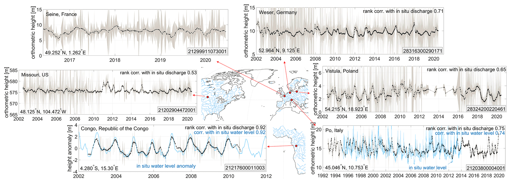
Figure 3High-rate altimetric water level over six selected rivers with different average width: Seine river (with average width of 170 m and 67 VSs) in France, Missouri River in the US (with average width of 220 m and 61 VSs), Congo River in the Republic of the Congo (with average width of 2700 m and 59 VSs), Weser river in Germany (with average width of 100 m and 47 VSs), Vistula river in Poland (with average width of 50 m and 31 VSs) and Po River in Italy (with 350 m average with and 46 VSs). HydroSat IDs are provided in the bottom right of the graphs.
2.2 Data and methodology for generating water level time series
HydroSat water level time series are generated using the following datasets from different satellites: (1) Envisat GDR-v3, (2) Saral GDR T, (3) ICESat-2 ATL13 v3, (4) CryoSat-2 SIR GDR, (5) Jason-1 GDR data, (6) Jason-2 (PISTACH) GDR, (7) Jason-2 GDR data, (8) Jason-3 GDR data, (9) Sentinel-3A NTC data and (10) Sentinel-3B NTC data. In the following a detailed description of SR and HR products is provided.
2.2.1 Standard-rate water level time series from satellite altimetry
Whenever the satellite ground track crosses a hydrological object, a so-called virtual station (VS) can be determined. Boundaries of a VS are typically defined based on the type of the water body and the disposition of the altimetry track over the object. All measurements inside a lake or reservoir, for instance, could belong to the same virtual station. This is to assume that the along-track geoid height and altimetric corrections are properly known. In the case of a river, the assumption further implies that the spatial dynamics of the water body is locally negligible. Defining a VS, in effect, allows for reduction of random noise carried by the altimetric measurements.
HydroSat follows a rather flexible approach in defining a VS. The boundaries can be determined using static or dynamic shapefiles, a radial extent around a specific point of interest, or an intersection of the two. Furthermore, HydroSat employs auxiliary sources of information like the water occurrence frequency derived from Landsat imagery by Pekel et al. (2016). This allows for removal of measurements over areas with a water occurrence frequency below a certain threshold. Figure S1 shows the block diagram for generating SR water level time series, where the properties of the VS are the basic setup information to be introduced. Defining the VS setup is in fact the only subjective choice made throughout the whole procedure. Nevertheless, flexibility in defining a VS is tolerated as long as reproducibility of the results is guaranteed.
The altimetric water level is initially determined for each sample within the VS. First, range measurements are corrected for geophysical effects (solid Earth tide and pole tide) and path delays caused by the atmosphere (wet tropospheric, dry tropospheric and ionospheric). The water level is then calculated by subtracting the corrected range from the satellite altitude. In the next step, the reference height is changed to geoid according to static gravity field models from XGM2019e (Pail et al., 2018), EGM2008 (Pavlis et al., 2012) or EIGEN6C3 (Förste et al., 2012). To ensure a robust estimation at each overpass, the median of orthometric heights inside the VS is chosen to be the representative height.
It is important to notice that regardless of the choice of the VS, retracker, corrections and statistics by which a typical altimetric water level time series is generated, the result may be affected by many outliers. As already mentioned, missions supporting OLTC and SAR mode are less likely to provide erroneous range measurements. However, neither the OLTC nor the delay Doppler concept is capable of compensating for all unwanted radar processes over inland water bodies. Their usefulness may even be restricted by a number of known factors, e.g., crossing angle for SAR missions. An outlier identification algorithm is, therefore, required to clean the final water level time series from erroneous measurements.
In order to identify the outliers, HydroSat uses an automated, data-driven outlier identification methodology designed within an iterative, non-parametric adjustment scheme. As indicated in Fig. S1, the inputs to the algorithm are the water level time series and stochastic information derived from a number of outlier indicators (e.g., standard deviation of along-track estimates within a VS). The algorithm uses singular spectrum analysis (SSA) for gap-filling, Savitzky–Golay filtering for smoothing and a specially developed outlier identification method. The identification method benefits from applying a local kernel derived based on a local definition of an outlier. The identified outliers are not discarded instantly. The overall scheme allows for a possible correction of the outlying estimation through a retracking method that identifies the leading edge by benefiting from prior information. Such possibility is assessed via comparison of the single water level estimations inside the VS with the water level estimation coming from an ensemble model. The model, which is a by-product of the outlier identification algorithm, is used to bound the search area for identifying the true leading edge of the waveform. After retracking, the newly estimated heights are verified by their similarity to the along-track pattern of outlier-free cycles.
It is important to notice that after rejecting or correcting the outlying measurements, HydroSat does not low-pass-filter the water level time series. It can therefore fully capture the high-frequency behavior within the limitations of satellite sampling. However, this strategy may come at the cost of a higher error level for some stations, e.g., the Mississippi River.
2.2.2 High-rate water level time series from satellite altimetry
In order to obtain a HR product and cope with the limitation of temporal sampling of single-satellite inland water monitoring, multi-mission altimetry is applied. The multi-mission altimetry for lake monitoring is now a standard approach practiced by various studies and data providers (Crétaux et al., 2013). Assuming that a lake surface is an equipotential surface allows even calibration studies to be performed over lakes. However, for multi-mission altimetry one challenge is posed by the inter-satellite biases, which impede a straightforward combination of water level measurements. Moreover, inaccurate atmospheric corrections (wet tropospheric) may cause large biases of several decimeters, which is even more pronounced for rivers due to inhomogeneous neighboring topography (Fernandes et al., 2014). Unlike lakes, multi-mission studies over rivers are very limited. Only a few studies have been dedicated to water level monitoring of rivers using a multi-mission approach with the focus on improving the temporal resolution (Tourian et al., 2016; Boergens et al., 2017). Here the challenge is to combine measurements from different missions at different locations with dissimilar dynamic behavior and hydraulic parameters. In general, HydroSat follows two different approaches for obtaining the HR product over lakes and rivers, outlined in the following sub-sections.
2.2.3 High-rate altimetric water level over lakes and reservoirs
HR lake and reservoir level time series are provided based on the well-known multi-mission concept. As already mentioned, however, the integration of single water level time series is hampered by unknown biases, typically referred to as inter-satellite biases. Studies have been performed to tackle the problem, some targeting the specific case of lakes and reservoirs. Crétaux et al. (2009) provide an overview of research studies aiming at quantifying the absolute altimeter bias of each satellite. They also establish an absolute calibration site over Lake Issyk-Kul in central Asia for estimating the absolute bias of altimetry satellites and retrackers. Bosch et al. (2014) conduct a global cross-calibration analysis over the oceans to estimate the so-called radial bias – defined as the overall error in an altimeter system – in a relative manner. These results are interpolated by Schwatke et al. (2015a) and applied over inland altimetry water level time series. In order to minimize other sources of bias, DAHITI applies identical retracker and geophysical corrections to all measurements. Wang et al. (2019) correct for inter-satellite biases based on a maximum likelihood approach either for two missions with overlapping periods or by introducing ICESat-2 as an intermediary for non-overlapping ones.
HydroSat resolves biases in a relative, generic, regional and mission-independent manner (see Fig. S2). First, SR water level time series are categorized into groups of temporally overlapping and non-overlapping time series. For a group of overlapping time series, relative biases are estimated by minimizing a cost function for the merged time series. The cost function represents the difference between the power content of individual SR time series. If stationarity holds, minimizing such a cost function ensures the estimation of a correct relative bias. If stationarity does not hold, or in the case that any unresolved bias remains (scenario 2), remotely sensed surface area time series are used to act as an anchor of biased time series, allowing for estimation of the relevant biases. Here, a 2-D cost function in surface-area–water-level coordinates is minimized within a Gauss–Helmert adjustment scheme. Such a cost function is also used in the case that measurements have no overlap (scenario 1), leading to bias-removed SR lake water level time series. It is important to notice that relative biases are not necessarily estimated between missions but between time series. This allows for consideration of the inaccuracies of geoid or altimetry corrections within one lake and over different tracks.
A relative solution is preferred because absolute estimation of biases requires along-track in situ measurements. The absolute inter-satellite biases over a specific region, on the other hand, are not necessarily applicable elsewhere due to inhomogeneity of correction models at the global scale. It shall also be mentioned that a great portion of lakes and reservoirs are monitored by a few altimetry missions, often times with less-than-sufficient periods of overlap. For instance, the long-term, overlapping, 10 d revisiting Jason series only monitor a small number of lakes given their coarse ground-track pattern. Our proposed method is therefore designed to be least affected by these restricting conditions.
2.2.4 High-rate altimetric water level over rivers
HR water level time series are obtained over rivers based on a method developed by Tourian et al. (2016), in which SR time series from individual altimetry missions are merged. This method allows the combination of all VSs from multiple satellite altimeters along a river hydraulically and statistically. As an example, Fig. S4 shows individual SR time series from different satellite missions along the Weser river in Germany. The idea of a HR product is to combine all these measurements for an arbitrary location along the river into a time series with improved temporal resolution.
Figure S3 shows the main processing steps of the densification method. Initially, the time lag due to streamflow between the altimetric virtual stations and the selected location is estimated. The average river width from satellite imagery together with the slope derived from satellite altimetry is used as input to a simple empirical hydraulic equation, which ultimately estimates the average flow velocity and thus the time lag (Tourian et al., 2016; Bjerklie et al., 2003)
Using the estimated time lag, the water level hydrographs of all measurements are shifted and stacked at the selected location. The stacked time series is then normalized according to its statistical distribution with the 3rd percentile assigned to 0 and the 85th percentile to 1. Outliers are then identified and removed from the normalized time series by Student's t test for a sliding time window of 1 month. All measurements outside the confidence limit are identified as outliers and removed from the measurements. The outlier-free normalized time series is then rescaled according to the statistical water level distribution of the selected site. Details on the implementation of the method can be found in Tourian et al. (2016).
Surface water storage is an important component of the hydrological cycle, and its accurate monitoring requires a realistic representation of the surface water extent (Elmi et al., 2016). Lack of such observations, however, has obscured the proper quantification of the freshwater storage and its spatio-temporal dynamics over many water bodies. With their global coverage and fine temporal resolution, satellite images provide an opportunity to monitor the surface water extent on a global scale and for almost all river basins. To this end, attempts have been made to generate dynamic water masks from different spaceborne missions with various temporal and spatial resolution. Some studies (Klein et al., 2017; Zhang and Gao, 2016; Khandelwal et al., 2017) take advantage of MODIS images to generate time series of surface water mask with a fine temporal resolution. Due to the coarse spatial resolution of MODIS images, however, small water bodies are excluded from their dataset. On the other hand, some studies (Donchyts et al., 2016; Yang et al., 2017; Pickens et al., 2020; Yao et al., 2019; Schwatke et al., 2020) use Landsat images to generate time series of surface water bodies. In comparison to MODIS, Landsat images have a better spatial resolution (30 m). Nevertheless, their coarse temporal resolution is a limiting factor for monitoring the fast dynamics of the water bodies.
Surface water area of any lake, reservoir and river reach can be extracted from an available global inland water dataset like the SRTM Water Body Data (SWBD) (NASA JPL, 2013), the Global Inundation Extent from Multiple Satellites (GIEMS) (Papa et al., 2010b) or the Global Surface Water Dataset (GSW) (Pekel et al., 2016). The derived surface water estimates are restricted to the temporal and spatial limitations of the initial dataset. In this vein, Zhao and Gao (2018) present the Global Reservoir Surface Area Dataset (GRSAD), which contains the monthly estimates of surface water area of the 6817 reservoirs between the years 1984–2015 obtained from the GSW dataset. The global reservoir bathymetry dataset (Li et al., 2020) presents the 3-D reservoir bathymetry of 347 global reservoirs integrating surface water area time series from the GRSAD and GSW dataset and altimetric water level measurements from the Hydroweb and G-REALM datasets and ICESat measurements.
Similar to altimetric water level time series, Hydroweb is the first website to provide lake surface area time series (Crétaux et al., 2011). Recently DAHITI (Schwatke et al., 2019) also boosted its database by the time series of lake area from optical satellite images (Table 2). Moreover, in recent years the Bluedot Observatory has provided reliable and timely information about surface area of lakes and reservoirs based on Sentinel-2 imagery, globally.
Table 2List of sources for providing time series of surface water extent from satellite imagery.
* Last access: 18 May 2022
While over lakes and reservoirs dynamic water masks exist (Table 2), to the best of our knowledge, no specific dataset for dynamic river masks has been developed so far. Given the complexities of extracting river water masks from stacks of satellite imagery, most efforts have been limited to the development of static water masks. Allen and Pavelsky (2018) and Yamazaki et al. (2019), for instance, have extracted river water masks through stacks of satellite images.
3.1 HydroSat products for surface water extent
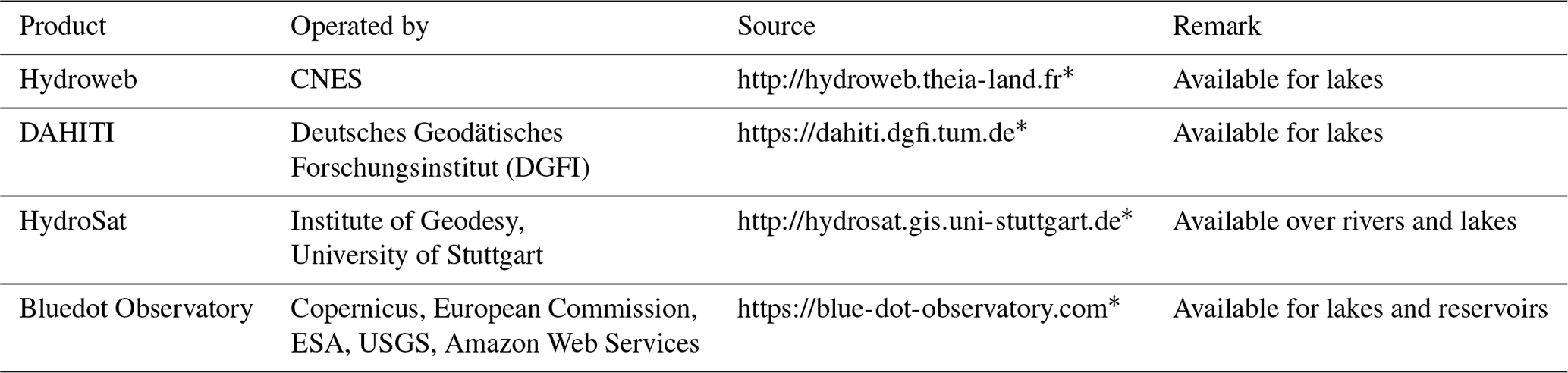
HydroSat provides surface water extent time series of lakes, reservoirs and river reaches from optical satellite images. From the obtained river reach area an effective river width can be determined by dividing the area by the length of the river reach. Figure 4 shows examples of time series of surface water extent for rivers and lakes derived from Landsat imagery in the Mississippi River basin.
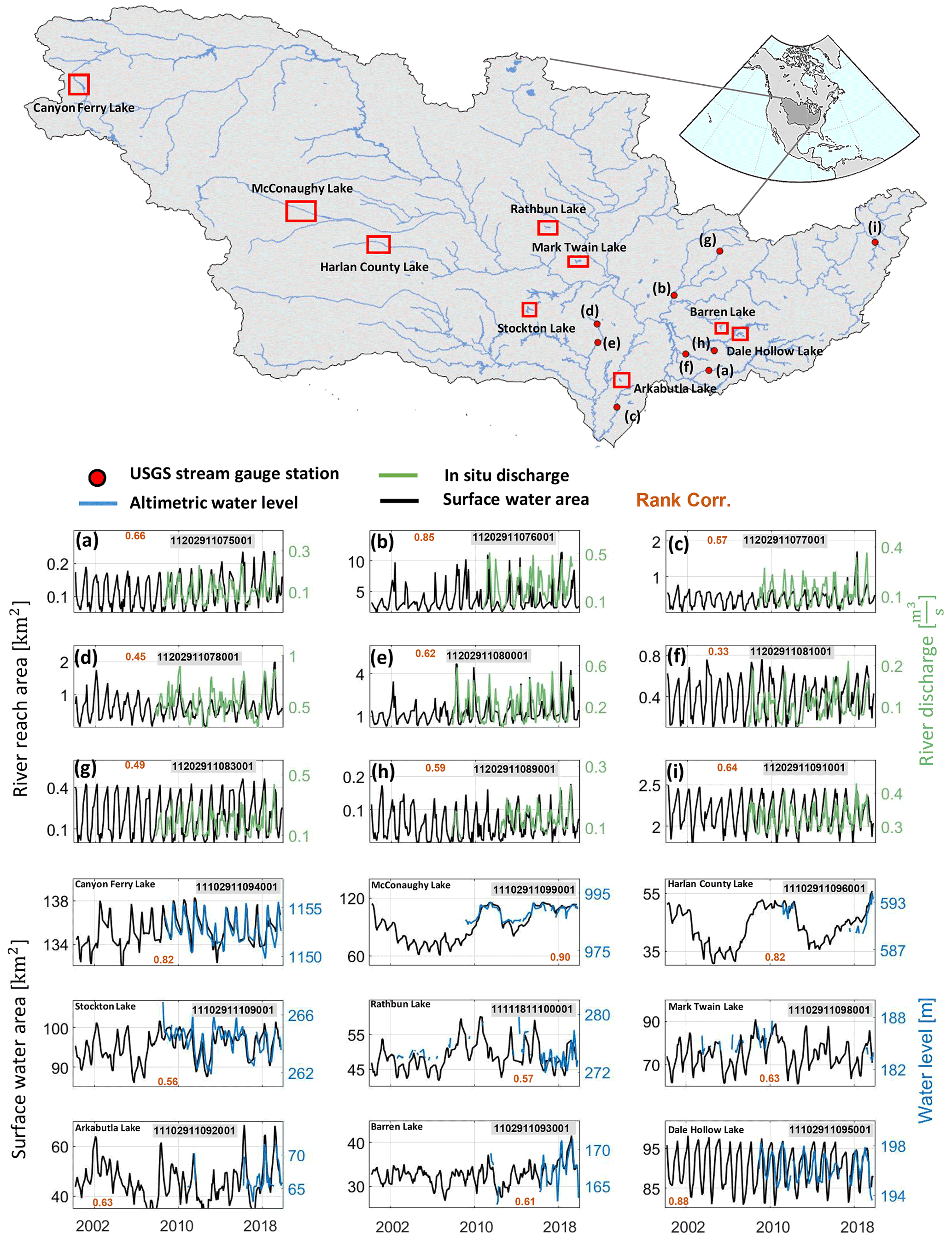
Figure 4Time series of river reach area of selected river reaches in the Mississippi River basin are in the middle panel.
To support an analysis of the performance of the algorithm, the time series of monthly river masks from nine river sections (average length of 10 km) in the Mississippi River basin are shown together with in situ discharge measurements from nearby USGS stream gauging stations. In all river reaches, we observe a relatively high rank correlation. However, in some river sections, as in Fig. 4g and f, the sections are too narrow (about 25 and 40 m), even for Landsat imagery with 30 m spatial resolution.
For lakes and reservoirs (second set of time series in Fig. 4), the time series of surface water area are compared with altimetric water level time series. For this comparison, nine small to medium-sized lakes or reservoirs in the Mississippi River basin are selected. In general, water level time series and surface water area show a good agreement represented by the reported rank correlation coefficients. For water bodies with smaller size, it is expected that the rank correlation decreases. As shown in Fig. 4, the rank correlation falls off to 0.57 and 0.61 for Rathbun and Barren lakes with average areas below 30 and 50 km2.
3.2 Data and methodology for generating surface water extent time series
HydroSat estimates of surface water extent are obtained from (1) MODIS MOD09Q1 imagery data and (2) the Monthly Water History product from the Global Surface Water dataset (Pekel et al., 2016). A classic approach to extract the water mask from optical images is to use pixel-based image segmentation algorithms, which are typically based on defining a threshold in the image pixel value histogram. While pixel-based algorithms are easy to implement, they fail to provide accurate water masks, especially over river reaches. The method performs well when the pixel values of the object and background create a combination of two normal distributions in the image histogram. This assumption, however, does not hold for the complicated river medium where the water body occupies only a small portion of the whole image. In fact, for a river reach, pixel values depend on several factors like water quality, roughness of water surface, chemical properties, load of sediments, vegetation canopy and the depth of the water column (Elmi, 2019). Therefore, along the shorelines the complicated combination of water, vegetation, and wet and dry soil within a pixel makes it almost impossible to find a unique threshold for distinguishing water from land. Region-based segmentation techniques, on the other hand, consider each pixel as an element of a larger region and use spatial information as well as pixel value to assign labels to the areas. Like other natural phenomena, water bodies show a strong spatial correlation in satellite images. Therefore, including contextual information can significantly improve the resulting water mask. Moreover, every pixel has a certain behavior during the time of monitoring, dominated by the seasonal cycle. Hence, in addition to spatial correlations, strong temporal correlations can be used as an additional source of information.
In order to derive a river mask, Elmi et al. (2016) estimate a maximum a posterior solution of a Markov random field (MAP-MRF), in which the spatial interactions between pixels and temporal variation in the pixel values are considered. Figure S5 (top panel) presents the block diagram of the proposed method. First, the cloud-covered images are removed. Initial water masks are then generated by applying a dynamic threshold. The procedure continues by developing the joint conditional models, rearranging the problem as one of energy minimization and developing a graph. In the next step the MAP solution is found by applying the graph cuts technique. Using the MAP solution, the initial water masks and the frequency coverage map are updated, allowing for modification of the already-developed graph. The final river mask is then obtained by finding the MAP solution for the modified graph. The uncertainty in the derived masks is estimated by marginalizing the final residual graph (Elmi et al., 2016; Elmi, 2019).
Although MODIS provides homogeneous daily snapshots of the Earth's surface for more than 20 years, its coarse spatial resolution is a limiting factor for generating dynamic river masks of relatively narrow river reaches and small lakes. To tackle this limitation, we use the Global Surface Water Dataset (GSWD) – developed by the European Commission's Joint Research Centre in the framework of the Copernicus program (Pekel et al., 2016) – as an alternative to MODIS data. Derived from Landsat data, GSWD is a unique product for analyzing the spatial and temporal distribution of water surfaces at the global scale over the past 3 decades. In its estimate of the surface water area, however, the dataset is subject to significant over- and underestimations. The main reason for underestimating the surface water area is the pixels labeled as no observations in the dataset. In the GSWD's Monthly Water History product, some pixels are contaminated due to the scan line corrector (SLC) failure of Landsat 7 and cloud coverage. Discarding all pixels with the no observations label leads not only to an underestimation of the area, but also to the generation of an erroneous water mask. On the other hand, a high noise level in the Landsat images might be the main reason for a possible overestimation of surface water extent. To generate enhanced dynamic water masks from this dataset, the algorithm described in Fig. S5 (bottom panel) is followed. The algorithm performs similar steps as for MODIS, relying on the GSWD masks instead of the original images.
Global observation of total water storage change is vital for understanding the water cycle and climate system dynamics. The variations in water storage indirectly reflect the Earth's energy storage, ocean heat content, land surface water storage, and biogeochemical and ice-sheet response to global warming (Tapley et al., 2019; Famiglietti, 2004). Water storage variation, both globally and regionally, influences our societies as it affects agricultural, industrial and domestic water use. Moreover, the dynamics of lake and reservoir storage are a key parameter in studies about the global hydrological cycle. Nevertheless, for a long time, monitoring of terrestrial and lake water storage changes relied on insufficient site measurements, which was costly and time-consuming. Moreover, on continental scales, it was not possible to map water storage because of the sparseness of the station networks (Rodell and Famiglietti, 1999). Furthermore, measurements of water storage changes by gauging groundwater level and soil water saturation changes are not reliable due to the lack of accurate storage coefficients (Strassberg et al., 2007; Riegger et al., 2012). Hydrological and land surface models have alleviated the problem to some extent. Such models estimate terrestrial water storage (TWS) and its components via simplification of real-world systems. The model outputs, however, are subject to high uncertainty and low accuracy due to the lack of global and systematic hydrological data (Jiang et al., 2014).
4.1 Terrestrial water storage anomaly
The GRACE launch in 2002 (Tapley et al., 2004) added unprecedented observations to the existing Earth monitoring system. The satellite program was jointly developed by the National Aeronautics and Space Administration (NASA) of the United States and the German Aerospace Center (DLR), which allowed for the recovery of the time-variable gravity field at catchment scales using the so-called low–low satellite-to-satellite tracking concept. The GRACE mission ended in October 2017 while providing over 15 years of near-continuous measurements of the Earth's gravity field. The monthly gravity variations are used to track mass changes in the hydrosphere, cryosphere and oceans, quantifying total water storage anomaly (TWSA). GRACE observations paved the way to monitor continental water storage, including deep soil water, for the first time. It contributed to various applications, including determining the natural and anthropogenic footprints in the global and regional water changes (Saemian et al., 2022), ice-sheet mass balance (Chen et al., 2009), ocean circulation, sea-level rise (Chen et al., 2013a; Jacob et al., 2012), atmospheric circulation patterns, drought monitoring (Long et al., 2013; Thomas et al., 2014), and flood forecasting (Reager et al., 2014). GRACE Follow-On (GRACE-FO), launched in May 2018, is continuing GRACE's legacy of monitoring Earth's temporal gravity field using the same constellation as GRACE while being additionally equipped with an experimental laser ranging interferometer (LRI).
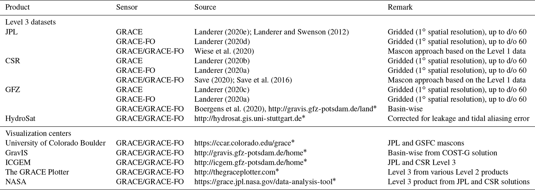
The collected GRACE and GRACE-FO measurements of each month are processed to estimate the Earth's gravity field in terms of spherical harmonics. The Science Data System (SDS), a joint US–German cooperation consisting of the Jet Propulsion Laboratory (JPL), the University of Texas Center for Space Research (UT-CSR) and the German Research Centre for Geosciences (GFZ), provides quality-controlled data from Level 0 (K-band ranging, KBR, range data) to Level 3 (grids). Moreover, Level 3 data from the mascon approach in terms of TWSA can be accessed from UT-CSR, JPL and the NASA Goddard Space Flight Center (NASA-GSFC), while the latter does not provide GRACE-FO observations. Other than Level 3 data, several centers help to visualize GRACE TWSA. The JPL and GSFC mascons, for instance, can be visualized using the Mascon Visualization Tool from the University of Colorado Boulder, and the basin-wise variability in TWS can be obtained from the Gravity over basins Information Service (GravIS) website. Furthermore, several data browsers allow the interactive retrieval of GRACE and GRACE-FO data, including the one developed within the International Center for Global Earth Models (ICGEM) project, the GRACE Plotter and the NASA Data Analysis Tool. Table 3 lists the abovementioned centers and products, including HydroSat.
Landerer (2020e); Landerer and Swenson (2012)Landerer (2020d)Wiese et al. (2020)Landerer (2020b)Landerer (2020a)Save (2020); Save et al. (2016)Landerer (2020c)Landerer (2020a)Boergens et al. (2020)Table 3List of centers which provide Level 3 TWSA from GRACE and GRACE-FO; d/o: degree and order.
* Last access: 18 May 2022
4.1.1 HydroSat products for terrestrial water storage anomaly
HydroSat provides time series of terrestrial water storage anomaly for major hydrological basins and also over grid cells. Figure 5 shows examples of terrestrial water storage anomaly for some selected basins. Figure 5 (top) shows the long-term trend of the major global hydrological basins. Figure 5 (bottom) compares the time series of GRACE and GRACE-FO TWSA estimation over the selected basin from HydroSat (black) with two mascon products: CSRv2 (red) and JPLv2 (blue). For visual simplicity and better comparison, only two common and updated mascon products have been selected. In general, in all catchments, TWSA estimation follows the two mascon products well. Minor discrepancies are observed over the Yangtze River basin and Murray–Darling, which can be explained due to the different GIA (glacial isostatic adjustment) models and low signal-to-noise ratio, respectively.
4.1.2 Data and methodology for generating terrestrial water storage anomaly
As input data HydroSat uses the ITSG-Grace2018 unconstrained gravity field model from the Institute of Geodesy at the Graz University of Technology (Mayer-Gürr et al., 2018; Kvas et al., 2019).
Figure S6 presents the scheme of the data processing handled in HydroSat to retrieve TWSA from GRACE Level 2 solutions. Each monthly solution contains the full hydrological, cryospheric and GIA signal in the form of fully normalized spherical harmonic (SH) coefficients, after removing the contributions from other phenomena like tides (ocean, solid Earth and atmospheric) and atmospheric and non-tidal oceanic mass changes.
To obtain TWSA, HydroSat applies several corrections on GRACE solutions, known as post-processing steps. The first-degree coefficients are added to the GRACE solutions, accounting for the movement of the Earth's center of mass (Swenson et al., 2007). Since GRACE estimations of the lowest-degree zonal harmonic coefficient are not accurate, we replace GRACE C2,0 and C3,0 by the coefficients derived from satellite laser ranging (SLR) data (Cheng et al., 2013). The real shape of the Earth is much closer to an ellipsoid than a sphere. Therefore, each solution is corrected from spherical to ellipsoidal coefficients following the method proposed by Li et al. (2017). To calculate the geoid anomalies, we remove the long-term (2004–2010) mean of spherical harmonics. Due to imperfect tidal models, GRACE SHs are contaminated by residual tidal aliasing error, a primary and a secondary one (Tourian, 2013). Therefore, HydroSat eliminates the primary and secondary tidal aliasing errors in the main tidal constituents, S1, S2, P1, K1, K2, M2, O2, O1 and Q1, from GRACE monthly solutions using a least-squares Fourier analysis (Tourian, 2013).
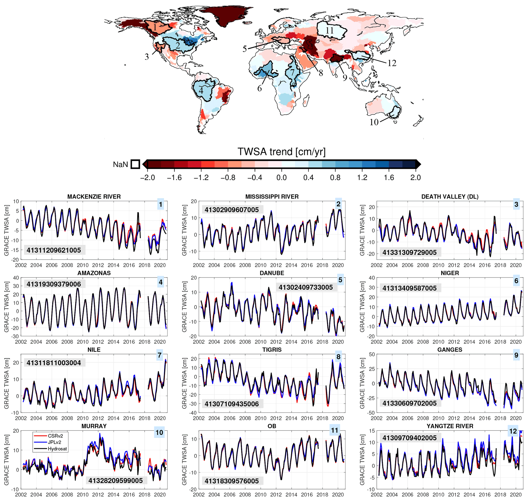
Figure 5Top: annual trend of TWSA over major global river basins from April 2002 to 2020. Selected basins are numbered on the map. The borders are defined based on the major river basins of the world of the Global Runoff Data Centre (GRDC; https://www.bafg.de/GRDC, last access: 18 May 2022). Bottom: time series of TWSA from GRACE and GRACE-FO for the selected basins, comparing the results from HydroSat, JPLv02 global mascons and CSRv02 global mascons. The corresponding HydroSat number for each basin is provided in the gray box.
Furthermore, the monthly solutions are contaminated by noise from different sources including the high-frequency noise in the spherical harmonic coefficients due to the orbit geometry and sensor noise. In order to reduce the high-frequency noise and retrieve mass changes, Gaussian filtering with a radius of 400 km is applied (Wahr et al., 1998). Moreover, to correct for leakage due to filtering, existing methodologies are employed, e.g., a data-driven approach proposed by Vishwakarma et al. (2017) and forward-modeling (Chen et al., 2013a). Finally, HydroSat corrects the GIA signal following A et al. (2012). The uncertainty for the GRACE-based TWSA at each month is estimated by propagating the calibrated error in the GRACE and GRACE-FO Level 2 solutions.
4.2 Lake and reservoir water storage anomaly
The variation in water height and surface area of lakes and reservoirs has been successfully monitored using spaceborne measurements, as demonstrated in previous studies. Table 4 lists some of these studies providing either time series of water volume change or lake and reservoir bathymetry.
Crétaux et al. (2011)Gao et al. (2012)Yao et al. (2018)Wang et al. (2018)Li et al. (2019)Busker et al. (2019)Schwatke et al. (2020)Li et al. (2020)Klein et al. (2021)Table 4Overview of studies providing time series of lake and reservoir water volume variations.

The mentioned studies follow almost the same strategy to generate water volume anomaly time series or a bathymetry map. In these studies, after collecting the simultaneous surface water area and level measurements, the empirical relationship between lake water level and area is developed. Then the water volume variations are estimated using the so-called end-area formula or pyramid formula.
4.2.1 HydroSat products for lake water storage anomaly
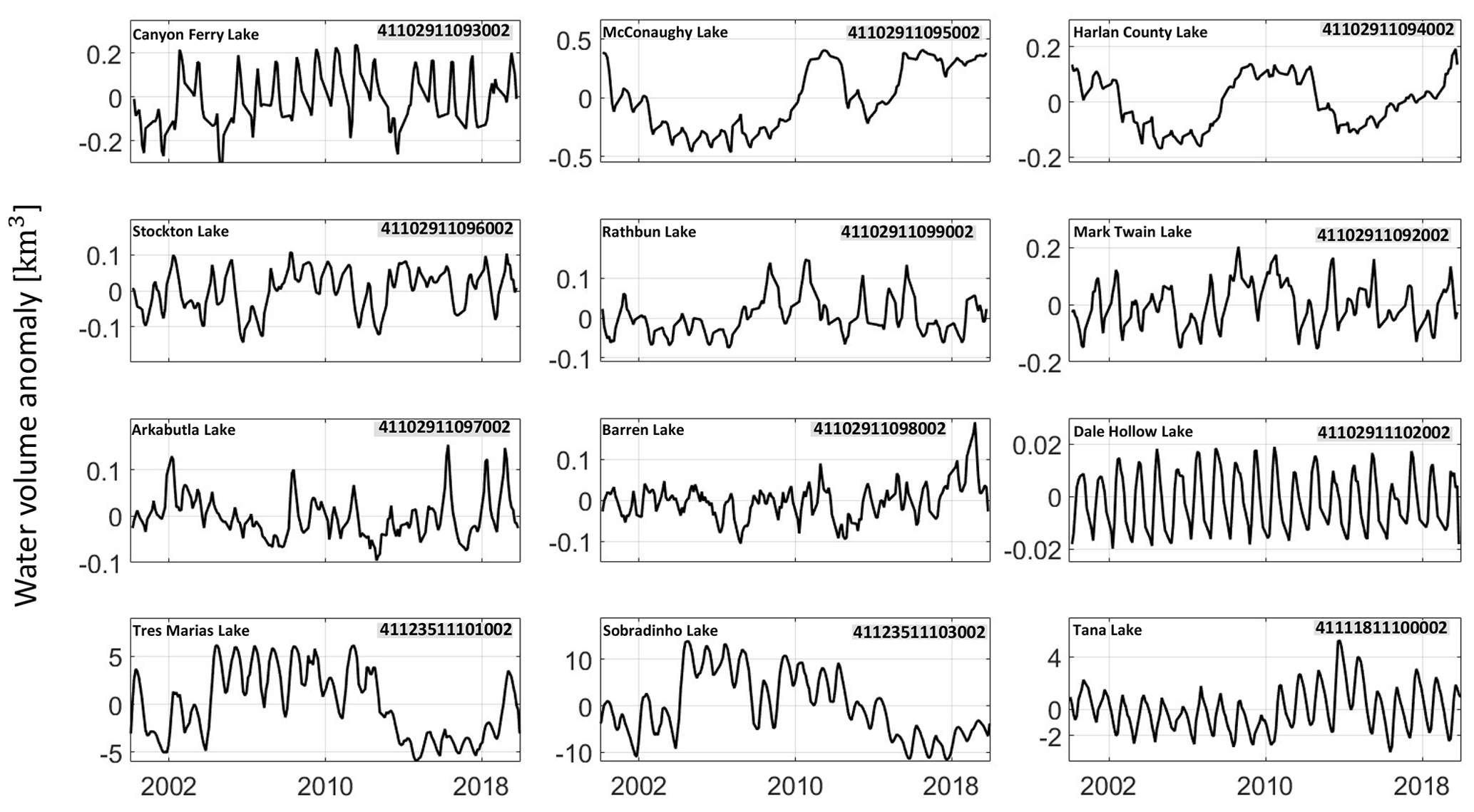
HydroSat estimates the water volume anomaly for lakes and reservoirs by combining water level and surface water area variation obtained from satellite altimetry and imaging measurements. Figure 6 shows selected time series of water volume anomaly for some small, medium and large lakes with different climate characteristics. A statistically representative joint time period for altimetry and imagery data is crucial to obtain a reliable estimate of water volume. For the Tana, Sobradinho and Dale Hollow lakes, for example, simultaneous surface water area and water level measurements are available for more than 10 years, resulting in a reliable area–volume model. Over Arkabutla Lake and Barren Lake, the joint time period is rather short but representative as it covers the entire statistical distribution of both variables. On the other hand, the time series of lake volume anomaly of the McConaughy, Harlan County, Rathbun and Mark Twain lakes carry mismodeling error as their joint time periods are short and non-representative of the entire distribution.
4.2.2 Data and methodology for generating lake and reservoir water storage anomaly
HydroSat follows a straightforward approach relying on a monotonic relationship of water level and surface area (Fig. S7). The algorithm starts by acquiring the water area from satellite imagery (explained in Sect. 3) and the time series of the water level (explained in Sect. 2). To derive the time series of the water volume anomaly and also the water-level–area–volume model, the following steps are performed:
-
generating monthly water level time series with the same temporal sampling as the surface area time series;
-
creating the scatterplot of the simultaneous surface water area and level and removing the blunders in the scatterplot;
-
defining the water surface-area–level model through either parametric or non-parametric approaches;
-
estimating the water volume variations by assuming that between two successive pairs of measurements (water level H and lake area S), the lake morphology is regular and has a pyramidal shape (Abileah et al., 2011)
-
obtaining the water-area–level–volume model.
Monitoring of river discharge, defined as the volume of water passing a river section in a given time, is a critically important part to understanding a broad range of science questions focused on hydrology, hydraulics, biogeochemistry and water resource management. Especially the river discharge quantification in ungauged basins anywhere and anytime is the holy grail of hydrology. River discharge reflects the drainage basin dynamics and affects environmental conditions like currents and hydrography in coastal waters; it is a function of precipitation and meteorological elements controlling evapotranspiration, geology, relief and vegetation.
Despite its importance, the publicly available in situ river discharge database has been declining steadily over the past decades due mainly to economic and political reasons. From about 8000 (pre-1970), the number of available gauging stations has decreased to fewer than 1000 (around the year 2015) (Lorenz et al., 2014, 2015; Tourian et al., 2017b).
Given the insufficient monitoring from in situ gauge networks, and without any outlook for improvement, spaceborne approaches come to the rescue. Satellite-based Earth observation with its global coverage has been demonstrated to be a potential alternative to in situ measurements. In the future, the SWOT mission with wide-swath altimetry is expected to attain global river discharge given its unprecedented temporal resolution; spatial coverage; and the synchronous availability of river height, width and slope (Biancamaria et al., 2016; Durand et al., 2016).
5.1 HydroSat products for river discharge
In HydroSat, discharge estimates are available from both altimetric river water level and imagery-based effective river width also in the two modes of standard rate (SR) and high rate (HR). While the SR product relies on standard temporal resolution of the spaceborne data, the HR data come with a higher temporal resolution through an assimilation process. To the best of our knowledge, there is no repository or website providing similar space-based river discharge estimates.
Figure 7 presents the discharge estimated from river width, using the stochastic quantile mapping function algorithm over four different river reaches along the Niger, Congo and Po rivers (Elmi et al., 2021). High Nash–Sutcliffe model efficiency coefficient (NSE) values for the Niger River reaches (Fig. 7a, b) show that the developed method can accurately estimate the discharge given that both discharge and width measurements have a representative statistical distribution in the training period. The performance of the method significantly decreases over the Congo River reach (Fig. 7c) mainly because of the complex relationship between river width and discharge in this part of the river. The performance of the algorithm over the Po River reach is only minimally acceptable (NSE = 0.13). Here, the discharge is not estimated accurately due to insufficient width measurements at high discharge and low signal-to-noise ratio of the same measurements. The obtained rating curve over the Po River, however, highlights the advantage of using a non-parametric model through the quantile mapping function compared to choosing a parametric model. With the help of the proposed method, spaceborne discharge estimates can be obtained for all non-active gauges in politically ungauged basins (see Gleason and Durand, 2020).

Figure 7Adopted from Elmi et al. (2021): four river reaches defined as case studies (a) and (b) are the river reaches over the Niger River; (c) is part of the Congo River, and (d) is selected over the Po River. Each case shows the estimated discharge (green dots), scatterplots of the simultaneous observations used for developing models and stochastic quantile mapping function.
Figure 8 shows an example of a HR river discharge time series over Niger River at Lokoja. The inputs to the dynamic system are the altimetric and in situ river discharges. During the period when the only source of observations is the in situ data (before 1992), the Kalman filter estimates a discharge that matches the in situ data with a relative RMSE of less than 2 % (not visible in the figure). After 1992, when altimetric river discharge is available, the Kalman filter is less dependent on the in situ data, leading to a relative RMSE up to 50 %. The validation over the entire Niger basin and 22 gauges along the main stem show an average correlation of 0.9, an average relative RMSE, a relative bias of about 15 % and a NSE greater than 0.5 for 15 gauges.
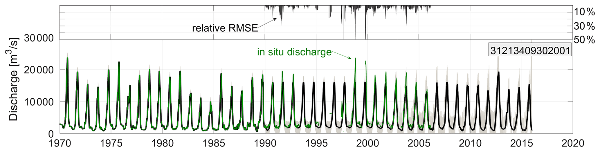
Figure 8Daily river discharge over the Niger River at Lokoja by assimilating altimetric discharge with available in situ data.
The proposed method is applicable in all river networks with available legacy in situ data. It allows a smoothed daily discharge time series to be obtained without data outages at any given location along a river.
5.2 Data and methodology for generating river discharge time series
The input data for generating both SR and HR river discharge are either SR or HR water level time series or the effective river width obtained from satellite imagery. In the following the methodology of generating discharge time series is described.
5.2.1 Standard-rate river discharge
Standard-rate river discharge Q at selected gauges can be estimated from space-based water level H (or river width W) measurements using an empirical relationship between river height (or width) and discharge (Kouraev et al., 2004; Birkinshaw et al., 2010). The most common form of this relationship is the so-called rating curve Q=F(H) or Q=F(W). Rating curves are conventionally generated for simultaneous measurements of space-based water level (or river width) and in situ river discharge. Once the model is developed, the discharge can be determined from water level or width measurements. The restriction however remains that for deriving a rating curve, simultaneous measurements are required, meaning the availability of in situ measurements during the satellite era.
Globally a great portion of existing gauges are not active during the satellite era, although they provide a wealth of legacy data. For such gauges, Tourian et al. (2013) suggest a statistical approach based on quantile mapping of in situ discharge and altimetry water level measurements. Since the quantile functions of discharge and river water level (width) have the same x axis (cumulative probability), it is possible to connect their y axis directly and obtain F(H) or F(W). As this approach does not involve the time coordinate explicitly, the requirement for synchronous datasets is obsolete. This is to say that the pre-satellite river discharge data records can be salvaged and turned into usable data for the satellite altimetry or imagery time frame.
The method is further improved by Elmi et al. (2021) to infer a non-parametric model for estimating the river discharge and its uncertainty. The algorithm employs a stochastic quantile mapping function scheme by iteratively (1) generating realizations of river discharge and height (width) time series using a Monte Carlo simulation, (2) obtaining a collection of quantile mapping functions by matching all possible permutations of simulated river discharge and height (width) quantile functions, and (3) adjusting the measurement uncertainties according to the point cloud scatter. The flowchart in Fig. S8 describes the procedure of SR discharge estimation using spaceborne river height or width.
5.2.2 High-rate river discharge
HydroSat provides high-rate (HR) river discharge time series based on the method developed by Tourian et al. (2017a) that goes beyond the conventional one-on-one relationship between virtual station (or reach) and (legacy) in situ station explored in SR discharge products. A multitude of altimetric discharge time series over a river network are used in this approach to estimate time series of daily river discharge. This is fundamentally done via assimilation of multiple altimetric discharge – the SR time series – and in situ measurements using a linear dynamic system. The dynamic system consists of a stochastic process model that benefits from the cyclostationarity of discharge. This model is informed by the covariance and cross-covariance generated out of old in situ data. The process model is then combined with observation equations fed by several altimetric and in situ discharge time series to form a linear dynamic system. Ultimately, the system is solved using the Kalman filter, followed by smoothing of the solutions using the Rauch–Tung–Striebel (RTS) scheme (Rauch et al., 1965). In fact, the Kalman filter produces an a posteriori discharge estimate with a likelihood function of discharge based on the available observations and the prior information derived from the stochastic process model. In the case of an observation gap, the posterior estimates rely on the stochastic process model and its cyclostationary mean discharge. Figure S9 represents the flowchart for estimating the HR river discharge. The implementation details of the method can be found in Tourian et al. (2017a).
The data are publicly available in the HydroSat database via http://hydrosat.gis.uni-stuttgart.de (last access: 23 May 2022). All time series in this paper are assigned a number, the so-called HydroSat ID, by which the time series can be found in the HydroSat database via the search field. In this database all data can be browsed, visualized and analyzed without registration. However, registration is required to download the data. A snapshot of all data (taken in April 2021) with a total of 10 810 time series (34 time series on surface water extent, 1323 time series on water level, 36 time series on river discharge and 463 time series on water storage anomaly) is available in GFZ Data Services, which is accessible at https://doi.org/10.5880/fidgeo.2021.017 (Tourian et al., 2021). Input data:
-
Envisat GDR-v3 data from https://doi.org/10.5270/EN1-ajb696a (European Space Agency, 2018)
-
Saral GDR T data from ftp://ftp-access.aviso.altimetry.fr/geophysical-data-record/ (last access: 18 May 2022)
-
ICESat-2 ATL13 L3A Inland Water Surface Height, Version 3 from https://nsidc.org/data/atl13 (last access: 18 May 2022)
-
CryoSat-2 SIR GDR data from ftp://science-pds.cryosat.esa.int/ (last access: 18 May 2022)
-
Jason-1 GDR data from ftp://ftp-access.aviso.altimetry.fr/geophysical-data-record/ (last access: 18 May 2022)
-
Jason-2 (PISTACH) GDR data from ftp://ftpsedr.cls.fr/pub/oceano/pistach/J2/IGDR/hydro/ (last access: 18 May 2022)
-
Jason-2 GDR data from ftp://ftp-access.aviso.altimetry.fr/geophysical-data-record/ (last access: 18 May 2022)
-
Jason-3 GDR data from ftp://ftp-access.aviso.altimetry.fr/geophysical-data-record/ (last access: 18 May 2022)
-
Sentinel-3A NTC data from https://scihub.copernicus.eu/ (last access: 18 May 2022)
-
Sentinel-3B NTC data from https://scihub.copernicus.eu/ (last access: 18 May 2022)
-
GRACE monthly ITSG-Grace2018 data from https://doi.org/10.5880/ICGEM.2018.003 (Mayer-Gürr et al., 2018)
-
GRACE-FO monthly ITSG-Grace2018 data from https://doi.org/10.5880/ICGEM.2018.003 (Mayer-Gürr et al., 2018)
-
MODIS MOD09Q1 data from https://ladsweb.modaps.eosdis.nasa.gov/ (last access: 18 May 2022)
-
Landsat-based water masks from https://global-surface-water.appspot.com/ (last access: 18 May 2022) (Pekel et al., 2016).
The development of repositories and services to provide global water cycle products from spaceborne sensors is getting more attention than ever before, which is motivated by the urgent need for more hydrological evidence, the absence of perspective for improving in situ data, the existence of an abundance of satellite missions, the prospect of cutting-edge missions such as the SWOT mission and also the promise of operational satellites in space. Such products support studies focused on understanding the water cycle and the Earth system in general. HydroSat provides the following water cycle quantities.
-
Surface water extent of lakes and rivers. HydroSat provides surface water extent time series of both lakes and rivers from optical satellite images. For generating dynamic water masks, region-based classification is employed, which benefits from the spatio-temporal behavior of pixel intensity. This allows us to deal with the complexities in extracting dynamic river masks. Moreover, such an algorithm setup allows a probabilistic water mask, leading to an estimate for surface water extent uncertainty to be obtained. While datasets of surface water extent variation over lakes are available from various data centers, HydroSat additionally provides time series of river width for major river basins. For a quality assessment, time series of surface water extent over lakes are compared with available in situ and or altimetric water level time series. Over rivers, such a quality assessment is predominantly done through comparing the time series against in situ river discharge.
-
Water level time series of lakes and river. HydroSat provides water level time series of rivers, lakes and reservoirs in two modes, standard rate (SR) and high rate (HR), with their uncertainty estimates. For water level time series HydroSat uses an automated, data-driven outlier rejection methodology designed within an iterative, non-parametric adjustment scheme. The outlier-free measurements form the final time series without any further smoothing. While water level time series over inland water bodies are available from similar data centers, HydroSat additionally provides HR water level time series over rivers through densifying individual SR time series along a river. For the HR products over the lakes, inter-satellite biases are removed through a hybrid approach by incorporating lake surface area information. The quality of water level time series is assessed through a validation against in situ water level or proxy data like river discharge, river width or lake surface area.
-
Terrestrial water storage anomaly. HydroSat provides terrestrial water storage anomaly (TWSA) time series and its uncertainty in the form of equivalent water height over major global river basins using GRACE and GRACE-FO observations. To estimate TWSA time series from Level 2 data (spherical harmonics up to the 96th degree and order), the C2,0 and C3,0 are replaced, and the first degree is added from the corresponding SLR estimates. Moreover, ellipsoidal and GIA correction is followed by a smoothing Gaussian filter with a radius of 400 km. The final TWSA in HydroSat is corrected for tidal aliasing error and leaked signals. For the field product, the Gaussian filtering is applied together with a de-striping filter, and leakage is corrected using the forward modeling approach. The quality of TWSA time series is assessed through a comparison with two mascon products, CSR RL06 version 02 and JPL RL06 version 02.
-
Water storage anomaly of lakes and reservoirs. HydroSat provides time series of surface water storage anomaly for lakes and reservoirs using the time series of water level and surface area measurements. For developing the surface-water-level–area–volume model, the scatterplot of simultaneous water level and area measurements is obtained. HydroSat performs an iterative data snooping procedure to obtain a reliable empirical relationship between surface water level and area. In this way, the quality of the obtained time series of water storage anomaly is ensured since the non-representative measurements are eliminated.
-
River discharge estimates for large and small rivers. HydroSat provides SR and HR river discharge estimates together with their uncertainties. To obtain the SR products, HydroSat relies on a non-parametric quantile mapping approach that salvages gauging stations that are no longer updated with in situ measurements. Since no model assumptions are required under the non-parametric approach, the HydroSat discharge time series are less contaminated by mismodeling. For the uncertainty estimation HydroSat applies a stochastic quantile mapping function algorithm supported by a Monte Carlo simulation. The availability of enough SR time series over a river network allows the approximation of the spatio-temporal dynamics of a river system by a linear dynamical system. The HR products are the solutions of such a dynamic system by Kalman filters obtained with up to daily temporal resolution at potentially any location along the river. For the quality assessment, SR and HR discharge time series are compared with in situ and spatial river discharges, water levels and river widths.
The above geometric hydrological variables are unique as they provide key elements of the water cycle in many gauged and ungauged regions around the world. They can directly be used in hydrological modeling, either as inputs or for calibration purposes. Global hydrological modeling has been improved in terms of modeled processes, leading to a better recognition of modeling uncertainties. Such recognition clearly signals that the modeling uncertainties are not reduced. To reduce the uncertainty, one solution is indeed to use the best available input data for modeling. Space-based data together with process knowledge allow realistic modeling of water flows and storages in the different compartments. Moreover, spaceborne measurements can be used to calculate indicators of the past and future state of the global freshwater system to assess risks under 1.5 and 2 ∘C global warming and support decision-making (Döll et al., 2018).
In addition, variables of water level, surface water storage anomaly and surface water extent support downscaling of mass transport monitoring in time and space. The success of GRACE has created a new demand for scientists and decision-makers for a sustained observation of the terrestrial water storage change (Pail et al., 2015). Although the utility of GRACE data has been mainly limited to large catchments, understanding of water storage changes in regions with some local weak signatures plays an important role within the Earth system and the sustainable development of water resources (Lorenz et al., 2015). Therefore, an urgent priority is to mitigate the spatial resolution limitation of GRACE through incorporating additional hydrological variables such as surface water storage and river and lake water level variation. This will improve in particular our understanding of the water cycle in many small vulnerable catchment areas with large populations.
Additional added value of the HydroSat data is their complementary role in the SWOT mission. Over rivers, SWOT will estimate discharge from multiple algorithms as well as consensus values computed over multiple individual algorithms (Stuurman and Pottier, 2020). The majority of algorithms are Bayesian, relying on prior data. Hydrological variables provided by HydroSat can effectively be used as potential prior information for each of the discharge algorithms through available water levels (SR and HR), river width from satellite imagery and discharge estimates (SR and HR). Over lakes and reservoirs, our estimates of surface water extent and volume anomaly will boost SWOT's estimates in terms of both temporal resolution and coverage. This supports studies aiming to understand long-term behavior of lakes and reservoirs.
The supplement related to this article is available online at: https://doi.org/10.5194/essd-14-2463-2022-supplement.
MJT conducted the project; wrote the majority of the paper; and together with OE and YS devised HydroSat, defined requirements, and designed the website's layout and features. OE wrote Sects. 3 and 4.2 and contributed to Sect. 5.1. YS developed the HydroSat website during his time at the University of Stuttgart. SB wrote Sect. 2.1 and 2.2.1. PS wrote Sect. 4.1. RS maintains the HydroSat website. NS reviewed the paper and contributed to HydroSat activities. All authors discussed the results, reviewed the manuscript and commented on it.
The contact author has declared that neither they nor their co-authors have any competing interests.
Publisher’s note: Copernicus Publications remains neutral with regard to jurisdictional claims in published maps and institutional affiliations.
The authors acknowledge Alireza Sahami, Apple Inc., for his valuable inputs within the early phase of HydroSat. The authors would also like to thank Thomas Götz, Institute of Geodesy, University of Stuttgart, for his support regarding the database and the server of the HydroSat database. The authors acknowledge the following data centers for providing satellite data:
-
Envisat GDR-v3 data from https://doi.org/10.5270/EN1-ajb696a (European Space Agency, 2018)
-
Saral GDR T data from ftp://ftp-access.aviso.altimetry.fr/geophysical-data-record/ (last access: 18 May 2022)
-
ICESat-2 ATL13 L3A Inland Water Surface Height, Version 3 from https://nsidc.org/data/atl13 (last access: 18 May 2022)
-
CryoSat-2 SIR GDR data from ftp://science-pds.cryosat.esa.int/ (last access: 18 May 2022)
-
Jason-1 GDR data from ftp://ftp-access.aviso.altimetry.fr/geophysical-data-record/ (last access: 18 May 2022)
-
Jason-2 (PISTACH) GDR data from ftp://ftpsedr.cls.fr/pub/oceano/pistach/J2/IGDR/hydro/ (last access: 18 May 2022)
-
Jason-2 GDR data from ftp://ftp-access.aviso.altimetry.fr/geophysical-data-record/ (last access: 18 May 2022)
-
Jason-3 GDR data from ftp://ftp-access.aviso.altimetry.fr/geophysical-data-record/ (last access: 18 May 2022)
-
Sentinel-3A NTC data from https://scihub.copernicus.eu/ (last access: 18 May 2022)
-
Sentinel-3B NTC data from https://scihub.copernicus.eu/ (last access: 18 May 2022)
-
GRACE monthly ITSG-Grace2018 data from https://doi.org/10.5880/ICGEM.2018.003 (Mayer-Gürr et al., 2018)
-
GRACE-FO monthly ITSG-Grace2018 data from https://doi.org/10.5880/ICGEM.2018.003 (Mayer-Gürr et al., 2018)
-
MODIS MOD09Q1 data from https://ladsweb.modaps.eosdis.nasa.gov/ (last access: 18 May 2022)
-
Landsat-based water masks from https://global-surface-water.appspot.com/ (last access: 18 May 2022) (Pekel et al., 2016).
This paper was edited by Christian Voigt and reviewed by Fangfang Yao, Vagner Ferreira and two anonymous referees.
A, G., Wahr, J., and Zhong, S.: Computations of the viscoelastic response of a 3-D compressible Earth to surface loading: an application to Glacial Isostatic Adjustment in Antarctica and Canada, Geophys. J. Int., 192, 557–572, https://doi.org/10.1093/gji/ggs030, 2012. a
Abileah, R., Vignudelli, S., and Scozzari, A.: A completely remote sensing approach to monitoring reservoirs water volume, Int. Water Technol. J., 1, 63–77, 2011. a
Allen, G. H. and Pavelsky, T. M.: Global extent of rivers and streams, Science, 361, 585–588, https://doi.org/10.1126/science.aat0636, 2018. a
Alsdorf, D. and Lettenmaier, D. P.: Tracking Fresh Water from Space, Science, 301, 1491–1494, https://doi.org/10.1126/science.1089802, 2003. a, b
Alsdorf, D. E., Rodriguez, E., and Lettenmaier, D. P.: Measuring surface water from space, Rev. Geophys., 45, RG2002, https://doi.org/10.1029/2006RG000197, 2007. a, b
Berner, E. K. and Berner, R. A.: Global environment: water, air, and geochemical cycles, Princeton University Press, ISBN 9780691136783, 2012. a
Berry, P. A. M., Garlick, J. D., Freeman, J. A., and Mathers, E. L.: Global inland water monitoring from multi-mission altimetery, Geophys. Res. Lett., 32, L16401, https://doi.org/10.1029/2005GL022814, 2005. a
Biancamaria, S., Lettenmaier, D. P., and Pavelsky, T. M.: The SWOT mission and its capabilities for land hydrology, Surv. Geophys., 37, 307–337, https://doi.org/10.1007/s10712-015-9346-y, 2016. a, b
Birkett, C. M.: The global remote sensing of lakes, wetlands and rivers for hydrological and climate research, in: Geoscience and Remote Sensing Symposium, 1995, IGARSS '95, Quantitative Remote Sensing for Science and Applications, International, 3, 1979–1981, https://doi.org/10.1109/IGARSS.1995.524084, 1995. a
Birkinshaw, S. J., O'Donnell, G. M., Moore, P., Kilsby, C. G., Fowler, H. J., and Berry, P. A. M.: Using satellite altimetry data to augment flow estimation techniques on the Mekong River, Hydrol. Process., 24, 3811–3825, https://doi.org/10.1002/hyp.7811, 2010. a
Bjerklie, D. M., Lawrence Dingman, S., Vörösmarty, C. J., Bolster, C. H., and Congalton, R. G.: Evaluating the potential for measuring river discharge from space, J. Hydrol., 278, 17–38, https://doi.org/10.1016/S0022-1694(03)00129-X, 2003. a
Boergens, E., Buhl, S., Dettmering, D., Klüppelberg, C., and Seitz, F.: Combination of multi-mission altimetry data along the Mekong River with spatio-temporal kriging, J. Geodesy, 91, 519–534, https://doi.org/10.1007/s00190-016-0980-z, 2017. a
Boergens, E., Dobslaw, H., Dill, R., Thomas, M., Dahle, C., Murböck, M., and Flechtner, F.: Modelling spatial covariances for terrestrial water storage variations verified with synthetic GRACE-FO data, Int. J. Geomath., 11, 24, https://doi.org/10.1007/s13137-020-00160-0, 2020. a
Bosch, W., Dettmering, D., and Schwatke, C.: Multi-mission cross-calibration of satellite altimeters: Constructing a long-term data record for global and regional sea level change studies, Remote Sensing, 6, 2255–2281, https://doi.org/10.3390/rs6032255, 2014. a
Busker, T., de Roo, A., Gelati, E., Schwatke, C., Adamovic, M., Bisselink, B., Pekel, J.-F., and Cottam, A.: A global lake and reservoir volume analysis using a surface water dataset and satellite altimetry, Hydrol. Earth Syst. Sci., 23, 669–690, https://doi.org/10.5194/hess-23-669-2019, 2019. a
Chen, J., Wilson, C., Blankenship, D., and Tapley, B.: Accelerated Antarctic ice loss from satellite gravity measurements, Nat. Geosci., 2, 859–862, https://doi.org/10.1038/ngeo694, 2009. a
Chen, J., Wilson, C., and Tapley, B.: Contribution of ice sheet and mountain glacier melt to recent sea level rise, Nat. Geosci., 6, 549–552, https://doi.org/10.1038/ngeo1829, 2013a. a, b
Cheng, M., Tapley, B. D., and Ries, J. C.: Deceleration in the Earth's oblateness, J. Geophys. Res.-Sol. Ea., 118, 740–747, https://doi.org/10.1002/jgrb.50058, 2013. a
Coss, S., Durand, M., Yi, Y., Jia, Y., Guo, Q., Tuozzolo, S., Shum, C. K., Allen, G. H., Calmant, S., and Pavelsky, T.: Global River Radar Altimetry Time Series (GRRATS): new river elevation earth science data records for the hydrologic community, Earth Syst. Sci. Data, 12, 137–150, https://doi.org/10.5194/essd-12-137-2020, 2020. a, b
Crétaux, J.-F., Calmant, S., Romanovski, V., Shabunin, A., Lyard, F., Bergé-Nguyen, M., Cazenave, A., Hernandez, F., and Perosanz, F.: An absolute calibration site for radar altimeters in the continental domain: Lake Issykkul in Central Asia, J. Geodesy, 83, 723–735, https://doi.org/10.1007/s00190-008-0289-7, 2009. a
Crétaux, J.-F., Jelinski, W., Calmant, S., Kouraev, A., Vuglinski, V., Bergé-Nguyen, M., Gennero, M., Nino, F., Rio, R. A. D., Cazenave, A., and Maisongrande, P.: SOLS: A lake database to monitor in the Near Real Time water level and storage variations from remote sensing data, Adv. Space Res., 47, 1497–1507, https://doi.org/10.1016/j.asr.2011.01.004, 2011. a, b, c
Crétaux, J.-F., Berge-Nguyen, M., Calmant, S., Romanovski, V. V., Meyssignac, B., Perosanz, F., Tashbaeva, S., Arsen, A., Fund, F., Martignago, N., Bonnefond, P., Laurain, O., Morrow, R., and Maisongrande, P.: Calibration of Envisat radar altimeter over Lake Issykkul, Adv. Space Res., 51, 1523–1541, https://doi.org/10.1016/j.asr.2012.06.039, 2013. a
Dickinson, R. E.: Modeling Evapotranspiration for Three-Dimensional Global Climate Models, in: Climate Processes and Climate Sensitivity, edited by: Hansen, J. E. and Takahashi, T., https://doi.org/10.1029/GM029p0058, 1984. a
Döll, P., Trautmann, T., Gerten, D., Schmied, H. M., Ostberg, S., Saaed, F., and Schleussner, C.-F.: Risks for the global freshwater system at 1.5 ∘C and 2 ∘C global warming, Environ. Res. Lett., 13, 044038, https://doi.org/10.1088/1748-9326/aab792, 2018. a
Donchyts, G., Baart, F., Winsemius, H., Gorelick, N., Kwadijk, J., and Van De Giesen, N.: Earth's surface water change over the past 30 years, Nat. Clim. Change, 6, 810–813, https://doi.org/10.1038/nclimate3111, 2016. a
Durand, M., Gleason, C. J., Garambois, P. A., Bjerklie, D., Smith, L. C., Roux, H., Rodriguez, E., Bates, P. D., Pavelsky, T. M., Monnier, J., Chen, X., Di Baldassarre, G., Fiset, J.-M., Flipo, N., Frasson, R. P. d. M., Fulton, J., Goutal, N., Hossain, F., Humphries, E., Minear, J. T., Mukolwe, M. M., Neal, J. C., Ricci, S., Sanders, B. F., Schumann, G., Schubert, J. E., Vilmin, L.: An intercomparison of remote sensing river discharge estimation algorithms from measurements of river height, width, and slope, Water Resour. Res., 52, 4527–4549, https://doi.org/10.1002/2015WR018434, 2016. a
Elmi, O.: Dynamic water masks from optical satellite imagery, Verlag der Bayerischen Akademie der Wissenschaften, München, ISBN 978-3-7696-5246-8, https://doi.org/10.18419/opus-10597, 2019. a, b
Elmi, O., Tourian, M. J., and Sneeuw, N.: Dynamic river masks from multi-temporal satellite imagery: An automatic algorithm using graph cuts optimization, Remote Sensing, 8, 1005, https://doi.org/10.3390/rs8121005, 2016. a, b, c
Elmi, O., Tourian, M. J., Bárdossy, A., and Sneeuw, N.: Spaceborne River Discharge From a Nonparametric Stochastic Quantile Mapping Function, Water Resour. Res., 57, e2021WR030277, https://doi.org/10.1029/2021WR030277, 2021. a, b, c
European Space Agency: RA-2 Geophysical Data Record. Version 3.0, ESA [data set], https://doi.org/10.5270/EN1-ajb696a, 2018. a, b
Famiglietti, J.: Rallying Around Our Known Unknowns: What We Don’t Know Will Hurt Us, Water 50/50, June 28, https://aquadoc.typepad.com/waterwired/2012/06/jay-famiglietti-rallying-around-our-known-unknowns-what-we-dont-know-will-hurt-us.html (last access: 21 May 2022), 2012. a
Famiglietti, J. S.: Remote Sensing of Terrestrial Water Storage, Soil Moisture and Surface Waters, in: The State of the Planet: Frontiers and Challenges in Geophysics, edited by: Sparks, R. and Hawkesworth, C., American Geophysical Union (AGU), https://doi.org/10.1029/150GM16, 2004. a
Fernandes, M. J., Lázaro, C., Nunes, A. L., and Scharroo, R.: Atmospheric Corrections for Altimetry Studies over Inland Water, Remote Sensing, 6, 4952–4997, https://doi.org/10.3390/rs6064952, 2014. a
Förste, C., Bruinsma, S. L., Flechtner, F., Marty, J., Lemoine, J.-M., Dahle, C., Abrikosov, O., Neumayer, H., Biancale, R., Barthelmes, F., and Balmino, G.: A preliminary update of the Direct approach GOCE Processing and a new release of EIGEN-6C, in: AGU Fall meeting abstracts, vol. 2012, pp. G31B–0923, https://gfzpublic.gfz-potsdam.de/pubman/faces/ViewItemFullPage.jsp?itemId=item_246439_1 (last access: 21 May 2022), 2012. a
Fu, L.-L. and Cazenave, A.: Satellite Altimetry and Earth Sciences: A Handbook of Techniques and Applications, International Geophysical series, ISBN 9780080516585, 2001. a
Gao, H., Birkett, C., and Lettenmaier, D. P.: Global monitoring of large reservoir storage from satellite remote sensing, Water Resour. Res., 48, W09504, https://doi.org/10.1029/2012WR012063, 2012. a
Gleason, C. J. and Durand, M. T.: Remote sensing of river discharge: A review and a framing for the discipline, Remote Sensing, 12, 1107, https://doi.org/10.3390/rs12071107, 2020. a
Jacob, T., Wahr, J., Pfeffer, W. T., and Swenson, S.: Recent contributions of glaciers and ice caps to sea level rise, Nature, 482, 514–518, https://doi.org/10.1038/nature10847, 2012. a
Jiang, D., Wang, J., Huang, Y., Zhou, K., Ding, X., and Fu, J.: The review of GRACE data applications in terrestrial hydrology monitoring, Adv. Meteorol., 2014, 725131, https://doi.org/10.1155/2014/725131, 2014. a
Khandelwal, A., Karpatne, A., Marlier, M. E., Kim, J., Lettenmaier, D. P., and Kumar, V.: An approach for global monitoring of surface water extent variations in reservoirs using MODIS data, Remote Sens. Environ., 202, 113–128, https://doi.org/10.1016/j.rse.2017.05.039, 2017. a
Klein, I., Gessner, U., Dietz, A. J., and Kuenzer, C.: Global WaterPack – A 250 m resolution dataset revealing the daily dynamics of global inland water bodies, Remote Sens. Environ., 198, 345–362, https://doi.org/10.1016/j.rse.2017.06.045, 2017. a
Klein, I., Mayr, S., Gessner, U., Hirner, A., and Kuenzer, C.: Water and hydropower reservoirs: High temporal resolution time series derived from MODIS data to characterize seasonality and variability, Remote Sens. Environ., 253, 112207, https://doi.org/10.1016/j.rse.2020.112207, 2021. a
Kouraev, A. V., Zakharova, E. A., Samain, O., Mognard, N. M., and Cazenave, A.: Ob'river discharge from TOPEX/Poseidon satellite altimetry (1992–2002), Remote Sens. Environ., 93, 238–245, https://doi.org/10.1016/j.rse.2004.07.007, 2004. a
Kvas, A., Behzadpour, S., Ellmer, M., Klinger, B., Strasser, S., Zehentner, N., and Mayer-Gürr, T.: ITSG-Grace2018: Overview and evaluation of a new GRACE-only gravity field time series, J. Geophys. Res.-Sol. Ea., 124, 9332–9344, https://doi.org/10.1029/2019JB017415, 2019. a
Landerer, F.: CSR TELLUS GRACE-FO Level-3 Monthly Land Water-Equivalent-Thickness Surface Mass Anomaly Release 6.0 version 03, NASA [data set], https://doi.org/10.5067/GFLND-3AC63, 2020a. a, b
Landerer, F.: CSR TELLUS GRACE Level-3 Monthly Land Water-Equivalent-Thickness Surface Mass Anomaly Release 6.0 version 03, NASA [data set], https://doi.org/10.5067/TELND-3AC63, 2020b. a
Landerer, F.: GFZ TELLUS GRACE Level-3 Monthly Land Water-Equivalent-Thickness Surface Mass Anomaly Release 6.0 version 03, NASA [data set], https://doi.org/10.5067/TELND-3AG63, 2020c. a
Landerer, F.: JPL TELLUS GRACE-FO Level-3 Monthly Land Water-Equivalent-Thickness Surface Mass Anomaly Release 6.0 version 03, NASA [data set], https://doi.org/10.5067/GFLND-3AJ63, 2020d. a
Landerer, F.: JPL TELLUS GRACE Level-3 Monthly Land Water Equivalent Thickness Surface Mass Anomaly Release 6.0 version 03, NASA [data set], https://doi.org/10.5067/TELND-3AJ63, 2020e. a
Landerer, F. W. and Swenson, S. C.: Accuracy of scaled GRACE terrestrial water storage estimates, Water Resour. Res., 48, W04531, https://doi.org/10.1029/2011WR011453, 2012. a
Lettenmaier, D. P.: Observations of the Global Water Cycle – Global Monitoring Networks, Encyclopedia of Hydrological Sciences, Print ISBN 9780471491033, Online ISBN 9780470848944, https://doi.org/10.1002/0470848944.hsa181, 2006. a
Li, J., Chen, J., Li, Z., Wang, S.-Y., and Hu, X.: Ellipsoidal correction in GRACE surface mass change estimation, J. Geophys. Res.-Sol. Ear., 122, 9437–9460, https://doi.org/10.1002/2017JB014033, 2017. a
Li, X., Long, D., Huang, Q., Han, P., Zhao, F., and Wada, Y.: High-temporal-resolution water level and storage change data sets for lakes on the Tibetan Plateau during 2000–2017 using multiple altimetric missions and Landsat-derived lake shoreline positions, Earth Syst. Sci. Data, 11, 1603–1627, https://doi.org/10.5194/essd-11-1603-2019, 2019. a
Li, Y., Gao, H., Zhao, G., and Tseng, K.-H.: A high-resolution bathymetry dataset for global reservoirs using multi-source satellite imagery and altimetry, Remote Sens. Environ., 244, 111831, https://doi.org/10.1016/j.rse.2020.111831, 2020. a, b
Long, D., Scanlon, B. R., Longuevergne, L., Sun, A. Y., Fernando, D. N., and Save, H.: GRACE satellite monitoring of large depletion in water storage in response to the 2011 drought in Texas, Geophys. Res. Lett., 40, 3395–3401, https://doi.org/10.1002/grl.50655, 2013. a
Lorenz, C., Devaraju, B., Tourian, M. J., Riegger, J., Kunstmann, H., and Sneeuw, N.: Large-scale runoff from landmasses: a global assessment of the closure of the hydrological and atmospheric water balances, J. Hydrometeorol., 15, 2111–2139, https://doi.org/10.1175/JHM-D-13-0157.1, 2014. a
Lorenz, C., Tourian, M. J., Devaraju, B., Sneeuw, N., and Kunstmann, H.: Basin-scale runoff prediction: An Ensemble Kalman Filter framework based on global hydrometeorological data sets, Water Resour. Res., 51, 8450–8475, https://doi.org/10.1002/2014WR016794, 2015. a, b
Lvovitch, M.: The global water balance, Eos Trans. AGU, 54, 28–53, https://doi.org/10.1029/EO054i001p00028, 1973. a
Markert, K. N., Pulla, S. T., Lee, H., Markert, A. M., Anderson, E. R., Okeowo, M. A., and Limaye, A. S.: AltEx: An open source web application and toolkit for accessing and exploring altimetry datasets, Environ. Modell. Softw., 117, 164–175, https://doi.org/10.1016/j.envsoft.2019.03.021, 2019. a, b
Mayer-Gürr, T., Behzadpour, S., Kvas, A., Ellmer, M., Klinger, B., Strasser, S., and Zehentner, N.: ITSG-Grace2018: Monthly, Daily and Static Gravity Field Solutions from GRACE, ICGEM [data set], https://doi.org/10.5880/ICGEM.2018.003, 2018. a
NASA JPL: NASA Shuttle Radar Topography Mission Water Body Data Shapefiles & Raster Files, NASA EOSDIS Land Processes DAAC [data set], https://doi.org/10.5067/MEaSUREs/SRTM/SRTMSWBD.003, 2013. a
Okeowo, M. A., Lee, H., Hossain, F., and Getirana, A.: Automated generation of lakes and reservoirs water elevation changes from satellite radar altimetry, IEEE J. Sel. Top. Appl., 10, 3465–3481, https://doi.org/10.1109/JSTARS.2017.2684081, 2017. a
Pail, R., Bingham, R., Braitenberg, C., et al.: Observing Mass Transport to Understand Global Change and and to benefit Society: Science and User Needs-An international multidisciplinary initiative for IUGG, ISBN 978-3-7696-8599-2, 2015. a
Pail, R., Fecher, T., Barnes, D., Factor, J., Holmes, S., Gruber, T., and Zingerle, P.: Short note: the experimental geopotential model XGM2016, J. Geodesy, 92, 443–451, https://doi.org/10.1007/s00190-017-1070-6, 2018. a
Papa, F., Durand, F., Rossow, W. B., Rahman, A., and Bala, S. K.: Satellite altimeter-derived monthly discharge of the Ganga-Brahmaputra River and its seasonal to interannual variations from 1993 to 2008, J. Geophys. Res., 115, C12013, https://doi.org/10.1029/2009JC006075, 2010a. a
Papa, F., Prigent, C., Aires, F., Jimenez, C., Rossow, W. B., and Matthews, E.: Interannual variability of surface water extent at the global scale, 1993–2004, J. Geophys. Res.-Atmos., 115, D12111, https://doi.org/10.1029/2009JD012674, 2010b. a
Pavlis, N. K., Holmes, S. A., Kenyon, S. C., and Factor, J. K.: The development and evaluation of the Earth Gravitational Model 2008 (EGM2008), J. Geophys. Res.-Sol. Ea., 117, B04406, https://doi.org/10.1029/2011JB008916, 2012. a
Pekel, J.-F., Cottam, A., Gorelick, N., and Belward, A. S.: High-resolution mapping of global surface water and its long-term changes, Nature, 540, 418–422, https://doi.org/10.1038/nature20584, 2016 (data available at: https://global-surface-water.appspot.com/, last access: 18 May 2022). a, b, c, d
Pickens, A. H., Hansen, M. C., Hancher, M., Stehman, S. V., Tyukavina, A., Potapov, P., Marroquin, B., and Sherani, Z.: Mapping and sampling to characterize global inland water dynamics from 1999 to 2018 with full Landsat time-series, Remote Sens. Environ., 243, 111792, https://doi.org/10.1016/j.rse.2020.111792, 2020. a
Rauch, H. E., Tung, F., and Striebel, C. T.: Maximum likelihood estimates of linear dynamic systems, AIAA J., 3, 1445–1450, https://doi.org/10.2514/3.3166, 1965. a
Reager, J., Thomas, B., and Famiglietti, J.: River basin flood potential inferred using GRACE gravity observations at several months lead time, Nat. Geosci., 7, 588–592, https://doi.org/10.1038/ngeo2203, 2014. a
Riegger, J., Tourian, M. J., Devaraju, B., and Sneeuw, N.: Analysis of grace uncertainties by hydrological and hydro-meteorological observations, Journal of Geodynamics, 59, 16–27, https://doi.org/10.1016/j.jog.2012.02.001, 2012. a, b
Rodell, M. and Famiglietti, J.: Detectability of variations in continental water storage from satellite observation of time dependent gravity field, Water Resour. Res., 35, 2705–2723, https://doi.org/10.1029/1999WR900141, 1999. a
Rodell, M., Chen, J., Kato, H., Famiglietti, J., Nigro, J., and Wilson, C.: Estimating groundwater storage changes in the Mississippi River basin (USA) using GRACE, Hydrogeol. J., 15, 159–166, https://doi.org/10.1007/s10040-006-0103-7, 2006. a
Rodell, M., Beaudoing, H. K., L’Ecuyer, T. S., Olson, W. S., Famiglietti, J. S., Houser, P. R., Adler, R., Bosilovich, M. G., Clayson, C. A., Chambers, D., Clark, E., Fetzer, E. J., Gao, X., Gu, G., Hilburn, K., Huffman, G. J., Lettenmaier, D. P., Liu, W. T., Robertson, F. R., Schlosser, C. A., Sheffield, J., and Wood, E. F.: The observed state of the water cycle in the early twenty-first century, J. Climate, 28, 8289–8318, https://doi.org/10.1175/JCLI-D-14-00555.1, 2015. a, b
Saemian, P., Elmi, O., Vishwakarma, B., Tourian, M., and Sneeuw, N.: Analyzing the Lake Urmia restoration progress using ground-based and spaceborne observations, Sci. Total Environ., 739, 139857, https://doi.org/10.1016/j.scitotenv.2020.139857, 2020. a
Saemian, P., Tourian, M. J., AghaKouchak, A., Madani, K., and Sneeuw, N.: How much water did Iran lose over the last two decades?, Journal of Hydrology: Regional Studies, 41, 101095, https://doi.org/10.1016/j.ejrh.2022.101095, 2022. a
Save, H.: CSR GRACE and GRACE-FO RL06 Mascon Solutions v02. 2020, University of Texas [data set], https://doi.org/10.15781/cgq9-nh24, 2020. a
Save, H., Bettadpur, S., and Tapley, B. D.: High-resolution CSR GRACE RL05 mascons, J. Geophys. Res.-Sol. Ea., 121, 7547–7569, https://doi.org/10.1002/2016JB013007, 2016. a
Schwatke, C., Dettmering, D., Bosch, W., and Seitz, F.: DAHITI – an innovative approach for estimating water level time series over inland waters using multi-mission satellite altimetry, Hydrol. Earth Syst. Sci., 19, 4345–4364, https://doi.org/10.5194/hess-19-4345-2015, 2015a. a, b, c, d
Schwatke, C., Scherer, D., and Dettmering, D.: Automated extraction of consistent time-variable water surfaces of lakes and reservoirs based on landsat and sentinel-2, Remote Sensing, 11, 1010, https://doi.org/10.3390/rs11091010, 2019. a
Schwatke, C., Dettmering, D., and Seitz, F.: Volume Variations of Small Inland Water Bodies from a Combination of Satellite Altimetry and Optical Imagery, Remote Sensing, 12, 1606, https://doi.org/10.3390/rs12101606, 2020. a, b
Sneeuw, N., Lorenz, C., Devaraju, B., Tourian, M. J., Riegger, J., Kunstmann, H., and Bárdossy, A.: Estimating Runoff Using Hydro-Geodetic Approaches, Surv. Geophys., 35, 1333–1359, https://doi.org/10.1007/s10712-014-9300-4, 2014. a
Strassberg, G., Scanlon, B., and Rodell, M.: Comparison of seasonal terrestrial water storage variations from GRACE with groundwater-level measurements from the High Plains Aquifer (USA), Geophys. Res. Lett., 34, L14402, https://doi.org/10.1029/2007GL030139, 2007. a, b
Stuurman, C. and Pottier, C.: Level 2 KaRIn high rate river single pass vector product, Surface Water and Ocean Topography (SWOT) Project SWOT Product Description, https://podaac-tools.jpl.nasa.gov/drive/files/misc/web/misc/swot_mission_docs/pdd/D-56411_SWOT_Product_Description_L2_HR_PIXC_20200810.pdf (last access: 21 May 2022), 2020. a
Swenson, S., Chamber, D., and Wahr, J.: Estimating geocenter variations from a combination of grace and ocean model output, J. Geophys. Res., 113, B08410, https://doi.org/10.1029/2007JB005338, 2007. a
Tapley, B. D., Bettadpur, S., Ries, J. C., Thompson, P. F., and Watkins, M. M.: The Gravity Recovery and Climate Expriment: Mission overview and early results, Geophys. Res. Lett., 31, L09607, https://doi.org/10.1029/2004GL019920, 2004. a, b
Tapley, B. D., Watkins, M. M., Flechtner, F., Reigber, C., Bettadpur, S., Rodell, M., Sasgen, I., Famiglietti, J. S., Landerer, F. W., Chambers, D. P., Reager, J. T., Gardner, A. S., Save, H., Ivins, E. R., Swenson, S. C., Boening, C., Dahle, C., Wiese, D. N., Dobslaw, H., Tamisiea, M. E., and Velicogna, I.: Contributions of GRACE to understanding climate change, Nat. Clim. Change, 9, 358–369, https://doi.org/10.1038/s41558-019-0456-2, 2019. a
Thomas, A. C., Reager, J. T., Famiglietti, J. S., and Rodell, M.: A GRACE-based water storage deficit approach for hydrological drought characterization, Geophys. Res. Lett., 41, 1537–1545, https://doi.org/10.1002/2014GL059323, 2014. a
Tourian, M., Elmi, O., Shafaghi, Y., Behnia, S., Saemian, P., Schlesinger, R., and Sneeuw, N.: HydroSat: a repository of global water cycle products from spaceborne geodetic sensors, GFZ Data Services [data set], https://doi.org/10.5880/fidgeo.2021.017, 2021. a, b
Tourian, M. J.: Application of spaceborne geodetic sensors for hydrology, ISBN 978-3-7696-5132-4, https://doi.org/10.18419/opus-3929, 2013. a, b
Tourian, M. J., Sneeuw, N., and Bárdossy, A.: A quantile function approach to discharge estimation from satellite altimetry (ENVISAT), Water Resour. Res., 49, 4174–4186, https://doi.org/10.1002/wrcr.20348, 2013. a
Tourian, M. J., Tarpanelli, A., Elmi, O., Qin, T., Brocca, L., Moramarco, T., and Sneeuw, N.: Spatiotemporal densification of river water level time series by multimission satellite altimetry, Water Resour. Res., 52, 1140–1159, https://doi.org/10.1002/2015WR017654, 2016. a, b, c, d
Tourian, M. J., Schwatke, C., and Sneeuw, N.: River discharge estimation at daily resolution from satellite altimetry over an entire river basin, J. Hydrol., 546, 230–247, https://doi.org/10.1016/j.jhydrol.2017.01.009, 2017a. a, b
Tourian, M. J., Elmi, O., Mohammadnejad, A., and Sneeuw, N.: Estimating river depth from SWOT-Type observables obtained by satellite altimetry and imagery, Water, 9, 753, https://doi.org/10.3390/w9100753, 2017b. a
Vishwakarma, B. D., Horwath, M., Devaraju, B., Groh, A., and Sneeuw, N.: A data-driven approach for repairing the hydrological catchment signal damage due to filtering of GRACE products, Water Resour. Res., 53, 9824–9844, https://doi.org/10.1002/2017WR021150, 2017. a
Vörösmarty, C., Fekete, B. M., Meybeck, M., and Lammers, R. B.: Global system of rivers: Its role in organizing continental land mass and defining land-to-ocean linkages, Global Biogeochem. Cy., 14, 599–621, https://doi.org/10.1029/1999GB900092, 2000. a
Wahr, J., Molenaar, M., and Bryan, F.: The Time-Varibility of the Earth's gravity field: Hydrological and oceanic effects and their possible detection using GRACE, J. Geophys. Res., 103, 30205–30230, https://doi.org/10.1029/98JB02844, 1998. a
Wang, H., Chu, Y., Huang, Z., Hwang, C., and Chao, N.: Robust, long-term lake level change from multiple satellite altimeters in Tibet: Observing the rapid rise of Ngangzi Co over a new wetland, Remote Sensing, 11, 558, https://doi.org/10.3390/rs11050558, 2019. a
Wang, J., Song, C., Reager, J. T., Yao, F., Famiglietti, J. S., Sheng, Y., MacDonald, G. M., Brun, F., Müller Schmied, H., Marston, R. A., and Wada, Y.: Recent global decline in endorheic basin water storages, Nat. Geosci., 11, 926–932, https://doi.org/10.1038/s41561-018-0265-7, 2018. a
Wiese, D. N., Yuan, D.-N., Boening, C., Landerer, F. W., and Watkins, M. M.: JPL GRACE and GRACE-FO Mascon Ocean, Ice, and Hydrology Equivalent Water Height Coastal Resolution Improvement (CRI) Filtered Release 06 Version 02, NASA [data set], https://doi.org/10.5067/TEMSC-3JC62, 2020. a
Yamazaki, D., Ikeshima, D., Sosa, J., Bates, P. D., Allen, G. H., and Pavelsky, T. M.: MERIT Hydro: a high-resolution global hydrography map based on latest topography dataset, Water Resour. Res., 55, 5053–5073, https://doi.org/10.1029/2019WR024873, 2019. a
Yang, K., Yao, F., Wang, J., Luo, J., Shen, Z., Wang, C., and Song, C.: Recent dynamics of alpine lakes on the endorheic Changtang Plateau from multi-mission satellite data, J. Hydrol., 552, 633–645, https://doi.org/10.1016/j.jhydrol.2017.07.024, 2017. a
Yao, F., Wang, J., Yang, K., Wang, C., Walter, B. A., and Crétaux, J.-F.: Lake storage variation on the endorheic Tibetan Plateau and its attribution to climate change since the new millennium, Environ. Res. Lett., 13, 064011, https://doi.org/10.1088/1748-9326/aab5d3, 2018. a
Yao, F., Wang, J., Wang, C., and Crétaux, J.-F.: Constructing long-term high-frequency time series of global lake and reservoir areas using Landsat imagery, Remote Sens. Environ., 232, 111210, https://doi.org/10.1016/j.rse.2019.111210, 2019. a
Yeh, P., Swenson, S., Famiglietti, J., and Rodell, M.: Remote sensing of groundwater storage changes in Illinois using the Gravity Recovery and Climate Experiment (GRACE), Water Resour. Res., 42, W12203, https://doi.org/10.1029/2006WR005374, 2006. a
Zhang, S. and Gao, H.: A novel algorithm for monitoring reservoirs under all-weather conditions at a high temporal resolution through passive microwave remote sensing, Geophys. Res. Lett., 43, 8052–8059, https://doi.org/10.1002/2016GL069560, 2016. a
Zhao, G. and Gao, H.: Automatic correction of contaminated images for assessment of reservoir surface area dynamics, Geophys. Res. Lett., 45, 6092–6099, https://doi.org/10.1029/2018GL078343, 2018. a
- Abstract
- Introduction
- Inland water level from satellite altimetry
- Surface water extent from satellite imagery
- Water storage anomaly
- River discharge from space
- Data availability
- Summary, conclusion and outlook
- Author contributions
- Competing interests
- Disclaimer
- Acknowledgements
- Review statement
- References
- Supplement