the Creative Commons Attribution 4.0 License.
the Creative Commons Attribution 4.0 License.
 | 24 May 2022
Historical reconstruction of background air pollution over France for 2000–2015
Florian Couvidat
Anthony Ung
Laure Malherbe
Blandine Raux
Alicia Gressent
Augustin Colette
This paper describes a 16-year dataset of air pollution concentrations and air quality indicators over France. Using a kriging method that combines background air quality measurements and modeling with the CHIMERE chemistry transport model, hourly concentrations of NO2, O3, PM10 and PM2.5 are produced with a spatial resolution of about 4 km. Regulatory indicators (annual average, SOMO35 (sum of ozone means over 35 ppb), AOT40 (accumulated ozone exposure over a threshold of 40 ppb), etc.) are also calculated from these hourly data. The NO2 and O3 datasets cover the period 2000–2015, as well as the annual PM10 data. Hourly PM10 concentrations are not available from 2000 to 2007 due to known artifacts in PM10 measurements. PM2.5 data are only available from 2009 onwards due to the limited number of measuring stations available before this date. The overall dataset was evaluated over all years by a cross-validation process against background stations (rural, sub-urban and urban) to take into account the data fusion between measurement and models in the method. The results are very good for PM10, PM2.5 and O3. They show an overestimation of NO2 concentrations in rural areas, while NO2 background values in urban areas are well represented. Maps of the main indicators are presented over several years, and trends are calculated. Finally, exposure and trends are calculated for the three main health-related indicators: annual averages of PM2.5, NO2 and SOMO35. The DOI link for the dataset is https://doi.org/10.5281/zenodo.5043645 (Real et al., 2021). We hope that the publication of this open dataset will facilitate further studies on the impacts of air pollution.
- Article
(20576 KB) - Full-text XML
- BibTeX
- EndNote


Air pollution is a major environmental risk for human health and ecosystems in Europe. Over the past decades the European Union (EU) has put in place several measures to reduce anthropogenic emissions of pollutants. In response to emissions reductions, concentrations of SO2, NO2 and particles measured over Europe have shown a clear decrease since 1990 (EEA, 2018; EMEP, 2016).
The evolution of O3 trends is less clear despite the decrease in its precursors. The magnitude of high ozone episodes decreased, while annual average ozone levels measured at EMEP (European Monitoring and Evaluation Programme) stations were increasing in the 1990s and show a limited negative trend from 2002 onwards. As shown in the Tropospheric Ozone Assessment Report (Tarasick et al., 2019), this feature is generally attributed to the changing global tropospheric ozone baseline for which further hemispheric control strategies are needed. The same conclusions could be drawn from the Malherbe et al. (2017) study, which focused on France, with significant reductions in NO2 and particle concentrations and an increase in average O3 offset by a slight decrease in peak O3. Despite these reductions in emissions and pollutant concentrations (with the exception of the annual average O3), a proportion of French citizens are still exposed to concentrations above the EU limit and target value, and air quality in EU remains one of the main reasons for premature deaths (IHME, 2013).
As a complement to observations (which provide only partial spatial information), accurate, high-spatial-resolution and up-to-date air pollution maps are important information for assessing air pollution trends and exposure. They should provide geographically detailed information on the concentrations of air pollutants over the whole territory. These maps serve as a basis for informing citizens, designing and stratifying monitoring networks, supporting policy strategies, and measuring their impact. They are also used to estimate population exposure to air pollutants, which is essential for epidemiological studies.
On a European scale, different mapping approaches have been used to produce maps of pollutant concentrations. These maps can be obtained by modeling using a regional chemistry transport model (CTM) that simulates the concentration of pollutants over Europe. However, these models cannot always be used over the whole of Europe with a high resolution and have some biases and limitations in spatial representativeness. Regression methods (Briggs et al., 2000; Beelen et al., 2009) are also used at different scales. These stochastic modeling techniques develop statistical associations between potential “predictor variables” (land use, emission sources, topography) and measured pollutant concentrations in order to predict concentrations at an unsampled site. Other frequently used techniques are kriging techniques. These geostatistical techniques are based on the assumption that the data are spatially autocorrelated and therefore take into account the distances between measurements and the spatial structure of the variable. Different types of kriging are used to map the concentrations of air pollutants. Over France, kriging methods combining information from a regional CTM (CHIMERE; Mailler et al., 2017) and observations are produced daily by the Prev'air operational forecasting and mapping system for air quality (Rouïl et al., 2009). Since 2003 (for ozone) and 2005 (for PM10), the concentration maps simulated for the day before in Prev'air have been corrected each morning using observations. The kriging technique used in Prev'Air has evolved over time, and PM2.5 and NO2 concentrations are now also corrected for the day before. Today, a kriging of hourly observations with CHIMERE as external drift is applied to map NO2 and O3 concentrations. Since 2017, for the mapping of PM10 and PM2.5 concentrations, the method used is an hourly co-kriging of PM10 and PM2.5 data with CHIMERE as external drift. These choices are the results of successive studies that compared different kriging techniques (Malherbe and Ung, 2009, Beauchamp, 2015). A similar methodology was implemented for an earlier reconstruction of outdoor air pollution in Europe for the period 1989–2008 in Bentayeb et al. (2014). There are also ambient air pollution maps produced at European scale at 1 km resolution by the European Environment Agency but only for selected annual indicators and without consistency for multi-year reconstructions (Horálek et al., 2012, 2020). The Copernicus Atmosphere Monitoring Service has also produced European analyses since 2015, but again there is no multi-year consistency as these European maps are produced on an annual basis with gradually improving methodologies (Marécal et al., 2015). At the global scale, the Global Burden of Disease also makes available air pollution exposure maps; a recent update of the methodology was presented in (Shaddick et al., 2017), but the resolution is 0.1∘ or about 10 km.
The purpose of this paper and the associated datasets is to present and provide mapped data of O3, NO2, PM10 and PM2.5 concentrations at high spatial and temporal resolution and associated regulatory indicators covering the French metropolitan territory for the period 2000–2015 (2007–2015 and 2009–2015 for hourly concentrations of PM10 and PM2.5). The same kriging technique as in the Prev'air system is used to combine modeled and observed concentrations. Hourly concentrations of PM10, PM2.5, NO2 and O3 are produced and mapped over France, and these hourly data are then used to calculate and map European and French air quality standards.
Model outputs and measurements from the permanent monitoring network were combined by external drift kriging (Malherbe and Ung, 2009; Benmerad et al., 2017) to construct hourly concentration maps over France for a long period: 2000 to 2015. Details on the input data and methods used are described in the following paragraphs. From these corrected hourly concentration data, annual regulatory air quality maps are then constructed over France.
2.1 Monitoring data
Hourly measurements are extracted from validated reference datasets. For France, observations are extracted from the national air quality databases: BDQA (Base de Données de Qualité de l'Air) before 2013 and GEODAIR (https://www.lcsqa.org/fr/les-donnees-nationales-de-qualite-de-lair, last access: 19 May 2022) after 2013, as well as from the Airbase database (https://www.eea.europa.eu/themes/air/air-quality/map/airbase, last access: 19 May 2022) for other European countries from 2000 to 2012 and from air quality e-reporting (https://www.eea.europa.eu/data-and-maps/data/aqereporting-9, last access: 19 May 2022) from 2013 to 2015. All background monitoring data over the spatial domain are used in the kriging procedure except for stations with measurements above the 95 percentiles. This includes rural, suburban and urban stations but excludes industrial and traffic stations that are representative of very local concentrations and are difficult to reproduce in a national-scale mapping system. The number of background monitoring sites for each type of station and for each year is summarize in Table 1.
Table 1Number of background French monitoring sites for the years 2000 to 2015.
Until 1 January 2007, operational monitoring of PM10 and PM2.5 was carried out in France by automatic measuring systems of the TEOM (tapered element oscillating microbalance; PM10, PM2.5) or Beta (PM10) type. However, compared to the reference method EN 12341 (gravimetry), these systems underestimate the concentrations of particles. This is a known artifact related to the loss of semi-volatile compounds. To correct PM10 concentrations measured before 2007, a simple approach consists of applying a uniform correcting factor over France. This method is not suitable for correcting hourly or daily concentrations, but it has been shown to work well for annual average PM10 concentrations (Malherbe et al., 2017, Bessagnet et al., 2008). The factor (1.36) is a median value calculated on the PM10 data from “reference” sites (Bessagnet et al., 2008). As a consequence, for the period 2000 to 2006, the only PM10 indicator available is the annual average concentration. Concerning PM2.5, given the few reference measurements available before 2009, the reliability of even annual measurements is low. It was therefore decided to apply the kriging methodology only from the year 2009 onwards, which is when the change in measurement method had become widespread.
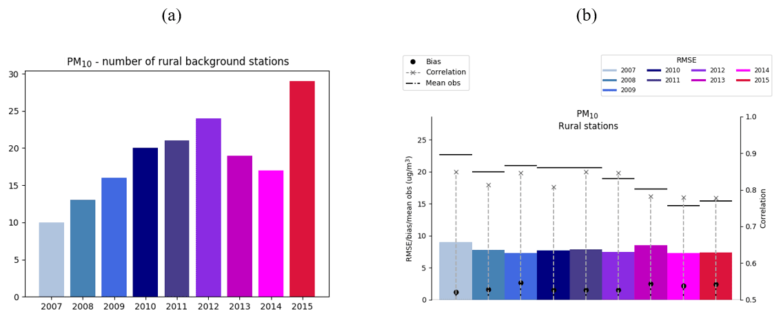
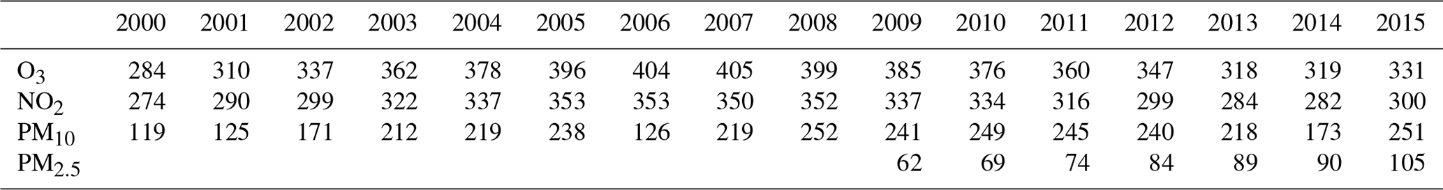
Figure 1PM10: statistical indicators calculated using cross-validation technique on daily mean PM10 values measured and estimated over rural background stations for the years 2007 to 2015. (a) Number of rural stations for each year. (b) Mean bias (black circles), RMSE (colored rectangles), correlation (grey crosses and the associated dashed lines) and mean observation (horizontal lines).
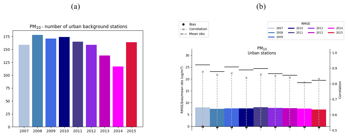
Figure 2PM10: statistical indicators calculated using cross-validation technique on daily mean PM10 values measured and estimated over URBAN background stations for the years 2007 to 2015. (a) Number of rural stations for each year. (b) Bias (black circles), RMSE (colored rectangles), correlation (grey crosses and the associated dashed lines) and mean observation (horizontal lines).

Figure 3PM2.5: statistical indicators calculated using cross-validation technique on daily mean PM2.5 values measured and estimated over rural background stations for the years 2009 to 2015. (a) Number of rural stations for each year. (b) Bias (black circles), RMSE (colored rectangles), correlation (grey crosses and the associated dashed lines) and mean observation (horizontal lines).
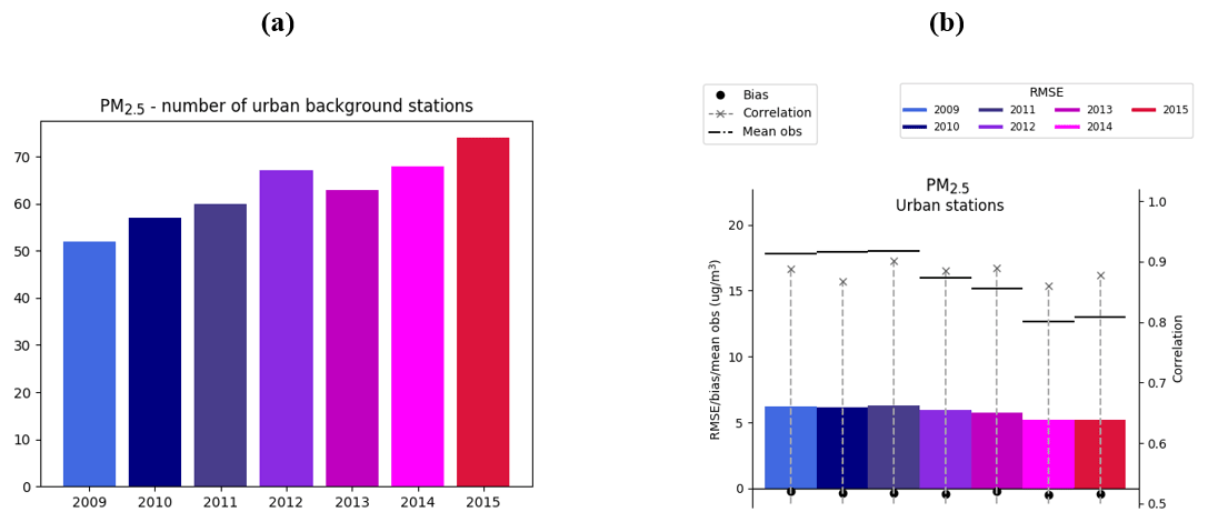
Figure 4PM2.5: statistical indicators calculated using cross-validation technique on daily mean PM2.5 values measured and estimated over URBAN background stations for the years 2009 to 2015. (a) Number of rural stations for each year. (b) Bias (black circles), RMSE (colored rectangles), correlation (grey crosses and the associated dashed lines) and mean observation (dotted horizontal lines).
2.2 CHIMERE simulations
The CHIMERE chemistry transport model (Couvidat et al., 2018) is used to estimate air pollution levels for metropolitan France with a resolution of about 4 km () over the years 2000 to 2015. This model has long been implemented and assessed in France as the main component of the national air quality forecasting and monitoring system PREV'AIR (Honoré et al., 2007). Two types of input data are used to simulate concentrations.
Prior to 2010, a configuration similar to the one used in the EURODELTA-Trends project (Colette et al., 2017) is used. The methodology of Colette et al. (2017) is used to reconstruct the emissions of the main air pollutants (non-methane volatile organic compound (NMVOC), NOx, CO, SO2, NH3 and primary PM): the annual emissions of each country, broken down by SNAP (Selected Nomenclature for reporting of Air Pollutants) sectors, are estimated using the GAINS (Greenhouse gases and Air pollution Interactions and Synergies) model (Amann et al., 2011) for the years 2000, 2005 and 2010 . To derive emissions for intervening years, sectorial results for 5-year periods are linearly interpolated. Meteorological data are simulated with the Weather Research and Forecast Model (WRF version 3.3.1; Skamarock et al., 2008) from 2000 to 2010.
For the period 2011 to 2015, year-to-year emissions of the main pollutants are taken from the cooperative program for the monitoring and evaluation of the long-range transmission of air pollutants in Europe (EMEP) available at https://www.ceip.at/webdab-emission-database/emissions-as-used-in-emep-models (last access: 19 May 2022). Annual meteorological data were provided by ECMWF with the Integrated Forecasting System (IFS) model with data assimilation.
For these two datasets, the spatialization of emissions over France is performed with a 1 km proxy based on the national bottom-up emission inventory (available at http://emissions-air.developpement-durable.gouv.fr/, last access: 19 May 2022) which feeds the CHIMERE emission pre-processor described in Mailler et al. (2017). Furthermore, Denier van der Gon et al. (2015) showed that primary PM emissions from residential wood burning can be underestimated by up to a factor of 2–3 over Europe because the emissions largely lack semi-volatile compounds. To compensate for this underestimation, a country correction factor determined from Denier van der Gon et al. (2015) is applied over the whole period.
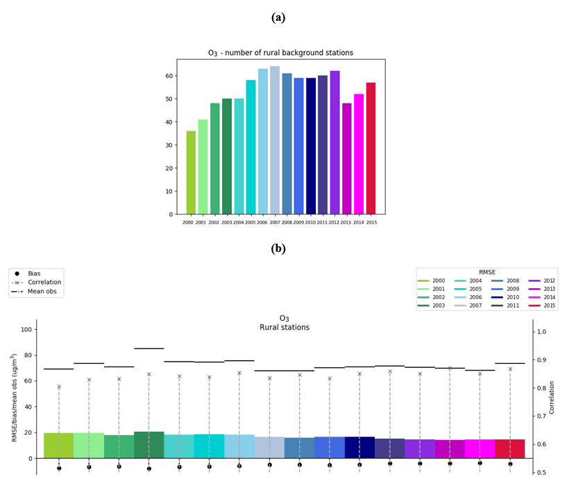
Figure 5O3: statistical indicators calculated using cross-validation technique on daily mean O3 values measured and estimated over rural background stations for the years 2000 to 2015. (a) Number of rural stations for each year. (b) Bias (black circles), RMSE (colored rectangles), correlation (grey crosses and the associated dashed lines) and mean observation (horizontal lines).
2.3 Kriging
Hourly atmospheric concentration fields are estimated by universal kriging, a geostatistical method. Kriging aims to estimate the value of a random variable (random process which describes the observations) at locations from the measurements. Kriging relies on the concept of spatial continuity, which implies that measurements that are close to each other will be more similar than distant measurements. In addition, kriging requires a good knowledge of the spatial structure of the interpolation domain which is represented by the variogram or co-variogram (second-order properties) of a random function (Goovaerts, 1997; Wackernagel, 1996; Chiles and Delfiner, 2012; Lichtenstern, 2013). Kriging involves deriving the linear combination of the observations which ensures the minimal estimation variance under a non-bias condition. At a point s0, the concentration estimate is given by Eq. (1).
where y(si), i=1…N, are the observed concentrations at sampling locations through the entire domain (unique neighborhood) or within a limited neighborhood of s0 (moving neighborhood), and λi, i=1…N, are the kriging weights.
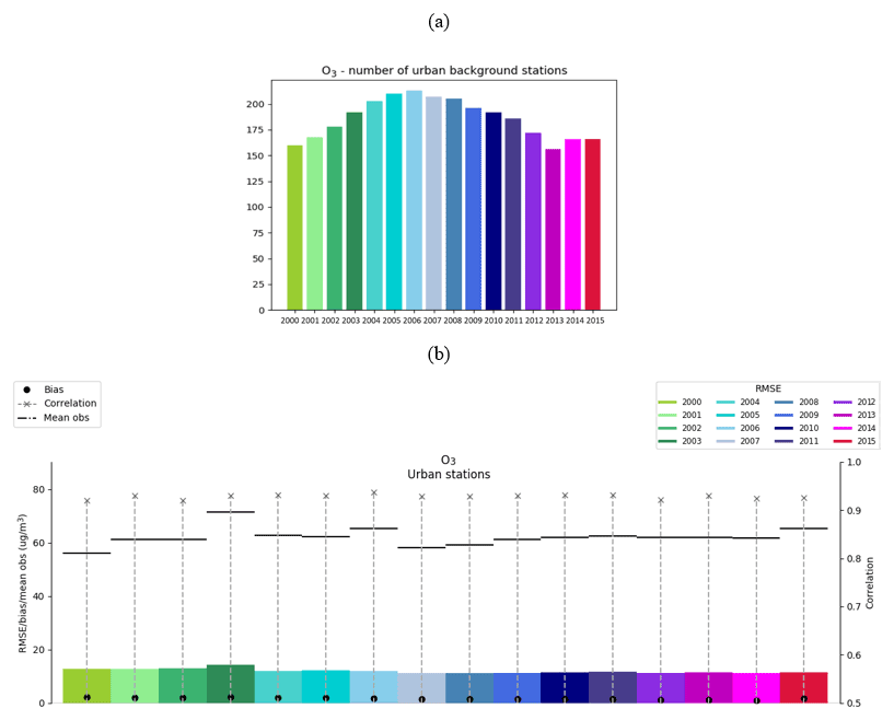
Figure 6O3: statistical indicators calculated using cross-validation technique on daily mean O3 values measured and estimated over URBAN background stations for the years 2000 to 2015. (a) Number of urban stations for each year. (b) Bias (black circles), RMSE (colored rectangles), correlation (grey crosses and the associated dashed lines) and mean observation (horizontal lines).
Among the kriging methods, the universal kriging (especially external drift kriging) allows us to consider additional information to make estimates more accurate. This approach is based on a linear regression with auxiliary variables and a spatial correlation of the residuals, and it allows us to combine simultaneously observations and additional information. The main hypothesis is that the global mean of the random variable is not constant through the domain, and it relies on explanatory variables. This kriging technique has been used for several years in monitoring air quality systems for spatial interpolation at the regional scale (PREV'AIR; Malherbe and Ung, 2009). For y(s0), which is the pollutant concentration to be estimated at a location s0, the hypothesis is a linear relation between y(s0) and the considered auxiliary variables as explained by Eqs. (2) and (3).
where m(s0) is the drift of the mean, are the coefficients of the linear regression, and are the auxiliary variables. ε corresponds to the stationary random process which is associated with a semi-variogram. In addition, the kriging weights must satisfy the drift condition described in Eq. 4.
In this work, kriging is performed with surface monitoring observations, and the drift is described by the outputs from the CHIMERE chemistry transport model. European stations located outside the French domain are included in the kriging to increase accuracy at the borders. The kriging is performed using a moving neighborhood as this allows for local adjustment of the relationship between the measurements and CHIMERE. The concentration at each grid point is estimated within a window of 80 monitoring sites. This number has been adjusted in previous studies by sensitivity tests (Benmerad et al., 2017; Beauchamp et al., 2017). In addition, smoothing is applied to avoid discontinuities in the map (Beauchamp et al., 2015); the smoothing methodology was adapted from Rivoirard and Romary (2011). The final output resolution is the same as for the CHIMERE model: approximately 4 km resolution ().
For PM10 (particles with a radius < 10 µm) and PM2.5 (particles with a radius < 2.5 µm) a co-kriging with external drift is applied. Co-kriging is an extension of kriging to the multivariate case. It allows the estimate of PM10 or PM2.5 concentrations by a linear combination of the two-variable data. The particularity of co-kriging is the use of the cross variance or semi-variance between the principal variable and the secondary variable. In the case of co-kriging with external drift, the simple and cross variograms are built based on residuals (De Fouquet et al., 2007). Co-kriging allows us to take into account the correlation between PM10 and PM2.5 and to improve consistency between PM10 and PM2.5 estimates (Beauchamp et al., 2015). This co-kriging also allows the PM2.5 estimate to benefit from the higher density of PM10 monitoring stations.
2.4 Output: regulatory air quality indicators
From the hourly kriged concentrations, several air quality indicators (regulatory and used in health impact assessments) are calculated and mapped over France. The complete list and definition of these indicators are given in Table 2.
Table 2Yearly regulatory air quality indicators from EU legislation or French legislation and usual indicators.
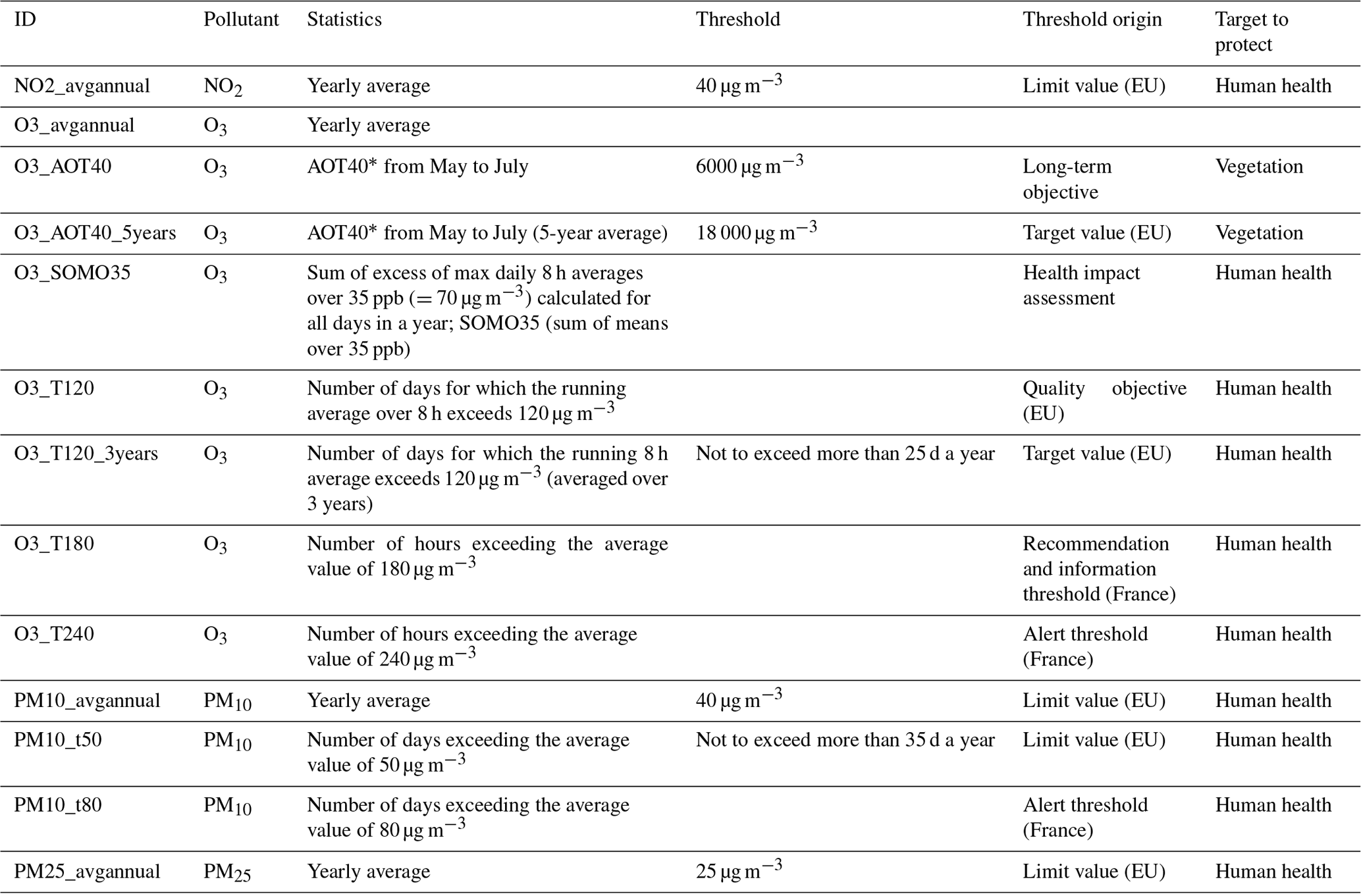
* AOT40 (expressed in µg m−3 h−1) means the sum of differences between hourly concentrations greater than 80 µg m−3 (=40 ppb or parts per billion) and 80 µg m−3 for a given period using only the 1 h values measured daily between 08:00 and 20:00 CET.
Usually the quality of the estimated concentration maps is assessed using statistical indicators that compare observations and estimated concentrations at the monitoring stations in the domain. Here, information of all background stations in the domain is already used to produce the maps. Therefore, for a fair comparison, the cross-validation method is used. The cross-validation method calculates the quality of the spatial interpolation for each measurement station point from all available information except the selected station point; i.e., it retains one data point and then makes a prediction at the spatial location of this point. This procedure is repeated for all measurement points in the available set, thus allowing the quality of the predicted values to be assessed at locations without measurements (provided they are within the area covered by the measurements).
It was noticed that the scores are systematically different at rural and urban stations (even though the kriging technique used here is not differentiated by the type of station). This is why the results of the cross-validation are described by pollutant and differentiated by station type (rural and urban types are presented here). Three statistical indicators are calculated on the basis of the daily average concentration: the mean bias, the root mean squared error (RMSE) and the Pearson correlation (r2). For each year, they are first calculated for the “left out” station, and then the median values over all stations are calculated.
Leave-one-out validation is a commonly used method in the air quality community (see, for example, ETC reports on air quality mapping (Horálek et al. 2017)) which is presently recommended by FAIRMODE (Janssen and Thunis, 2020). However, scores derived from the results of the leave-one-out validation might be influenced by areas where the density of sampling points is highest. For this reason, during the FAIRMODE project (Riviere et al., 2019), for which a kriging method similar to the one conducted here was conducted, a comparison has been performed between cross-validation results obtained by the leave-one-out cross-validation and cross-validation results obtained by the 5-fold cross-validation (cross-validation leaving 20 % of stations out). Results and related scores were very similar. We therefore decided to continue with the leave-one-out cross-validation process for the validation of our kriging results.
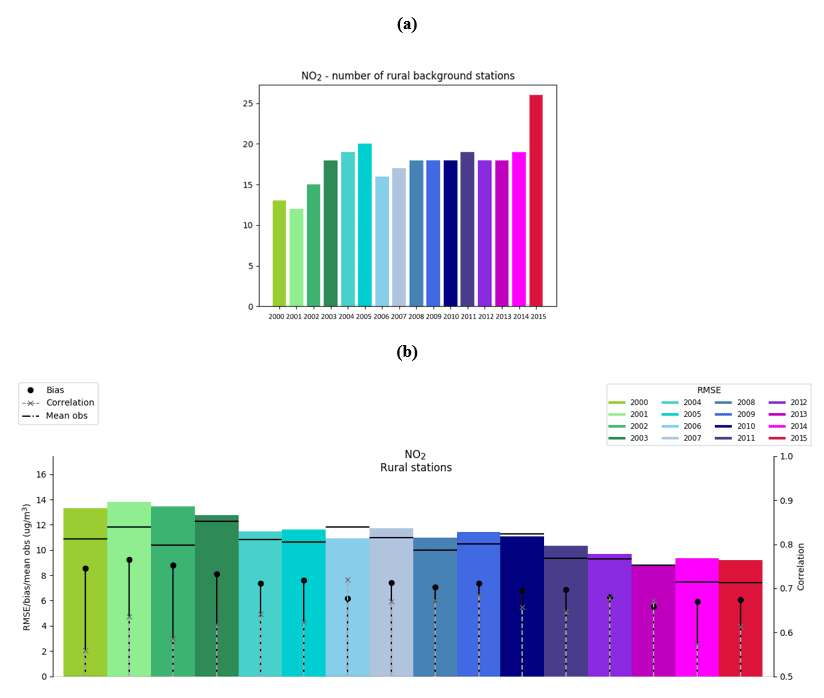
Figure 7NO2: statistical indicators calculated using cross-validation technique on daily mean NO2 values measured and estimated over rural background stations for the years 2000 to 2015. (a) Number of rural stations for each year. (b) Bias (black circles), RMSE (colored rectangles), correlation (grey crosses and the associated dashed lines) and mean observation (horizontal lines).
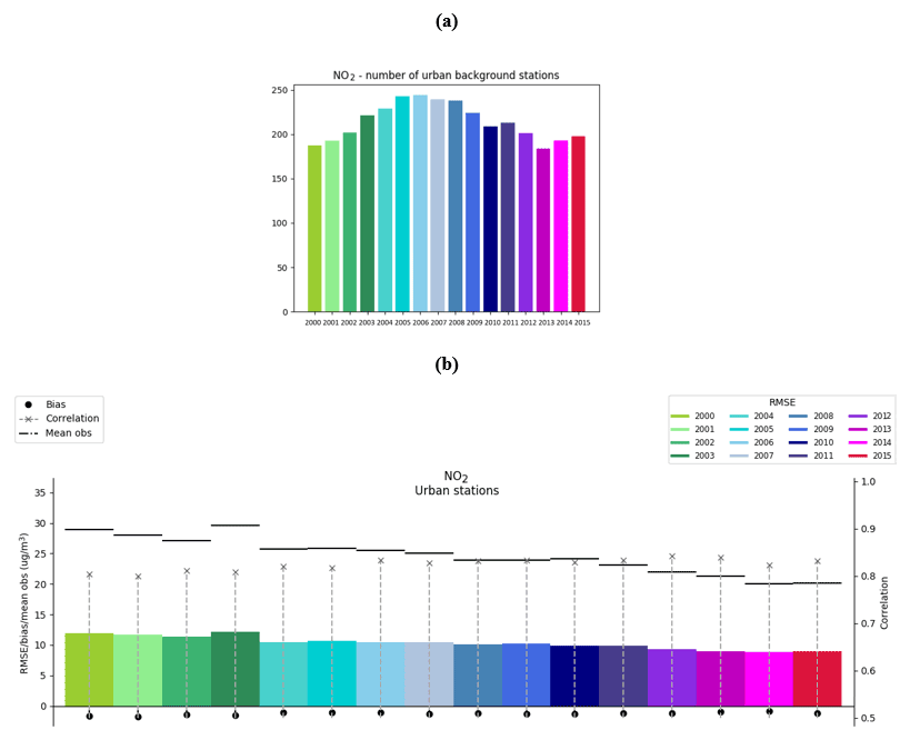
Figure 8NO2: statistical indicators calculated using cross-validation technique on daily mean NO2 values measured and estimated over URBAN background stations for the years 2000 to 2015. (a) Number of urban stations for each year. (b) Bias (black circles), RMSE (colored rectangles), correlation (grey crosses and the associated dashed lines) and mean observation (horizontal lines).
3.1 PM10
The scores show a good representation of the observations by the kriged data with correlations between 0.77 and 0.86 and RMSE of about 7 µg m−3, i.e., between 30 % and 50 % of the annual mean PM10 concentration. The mean biases are particularly low for urban stations with values below −1 %. For rural stations the average bias is less than + 3 µg m−3, i.e., less than + 15 %. The proportion between rural and urban stations varies between and . The larger number of urban stations allows a better capture of the spatial variability in concentrations in urban environments.
Looking at the evolution of the scores over the years for rural stations, the number of stations available first increases from 2009 to 2012 before decreasing until 2014. In 2015 a new increase in the number of stations in France begins. For urban stations, the decrease starts earlier (2010), but the evolution is the same. The temporal evolution of the scores generally follows the number of stations with higher correlations and smaller relative mean biases and RMSE when more stations are available. Indeed, the greater the number of stations there are, the more representative the kriging technique will be of the real spatial variability. There are exceptions, however, like in 2015 for rural stations, which had the second worst scores even though that year has the largest number of stations.
3.2 PM2.5
There are between a half and a third as many PM2.5 stations as PM10 stations. However, by using a co-kriging technique, the PM2.5 mapping also benefits from PM10 information so that the correlations, mean bias and RMSE are almost similar to the PM10 scores. The mean biases for rural stations do not exceed 20 % of the mean concentrations and are very low for urban stations (between 0 and − 3 %). As for PM10, this bias is systematically positive for rural stations (overestimation) and slightly negative over urban stations (underestimation). This is mainly related to the resolution of the data which smoothes the concentration gradients, giving a unique value for each grid (about 4 km horizontal resolution). For urban station, located close to PM2.5 precursor emissions and generally having high concentration values, this smoothing effect leads to an underestimation. For rural areas far from emission precursors, the opposite is observed.
The correlation is generally higher than 0.8, and the RMSE does not exceed 7 µg m−3 (at most 50 % of the annual mean concentration).
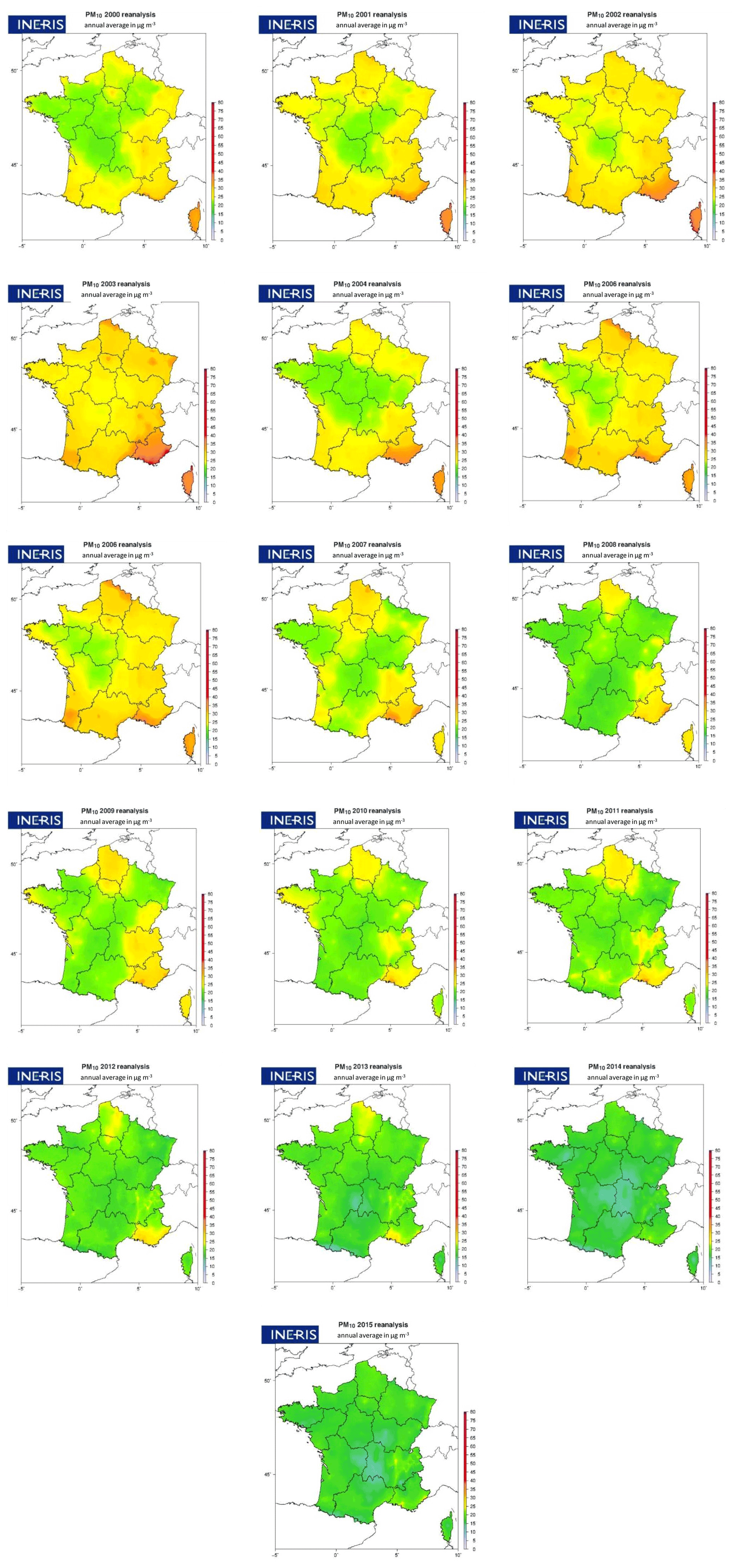
Figure 9PM10 annual mean concentrations from 2000 to 2015. Concentrations are obtained through a combination of regional modeling and observations.
3.3 O3
The comparison between estimated and observed ozone at rural stations shows good correlations (0.8 to 0.87), small relative mean negative biases (−4 % to −8 %) and low RMSE (around 20 % of the annual mean concentration). Between 2000 and 2007, the number of rural stations increased, resulting in improved modeled concentration maps. The small decrease in the number of stations after 2007 does not penalize the scores for these years.
The same conclusions can be drawn for the urban ozone scores. The higher number of urban stations even leads to slightly better scores, with correlations above 0.9 for all years and relative mean positive biases not exceeding 5 %. A satisfactory RMSE is also obtained for all years with values around 20 % of the annual mean concentration. It can be seen that the positive and negative biases are reverse with respect to the PM scores. Indeed, the highest O3 values are generally observed in rural areas where precursors have had time to produce O3 and where O3 destruction is lower than in urban areas. Therefore, the smoothing effect has the opposite effect to that of PM.
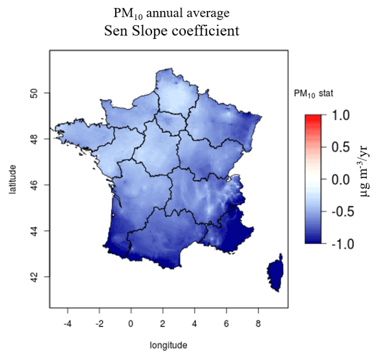
Figure 10Trends in PM10 annual mean concentration. Sen slope coefficient (µg m−3 yr−1) calculated over the period 2000–2015.
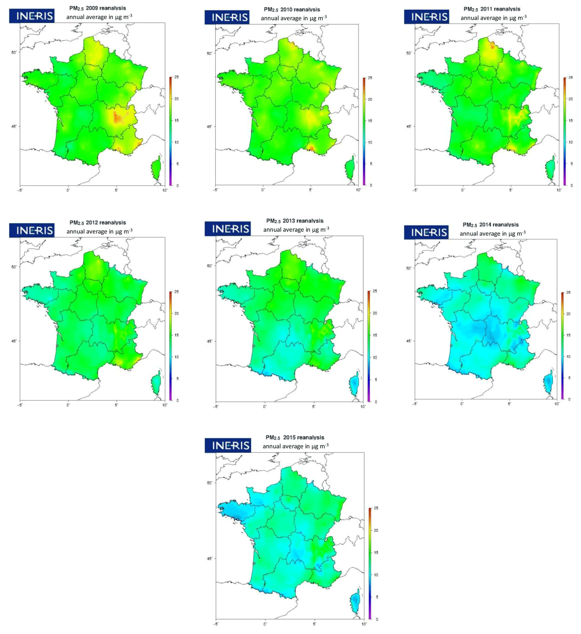
Figure 11PM2.5 annual mean concentrations from 2009 to 2015. Concentrations are obtained through a combination (kriging) of regional modeling and observations.
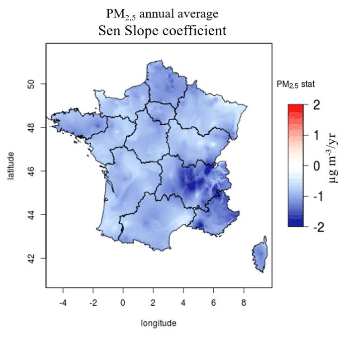
Figure 12Trends in PM2.5 annual mean concentration. Sen slope coefficients (µg m−3 yr−1) calculated over the period 2009–2015.
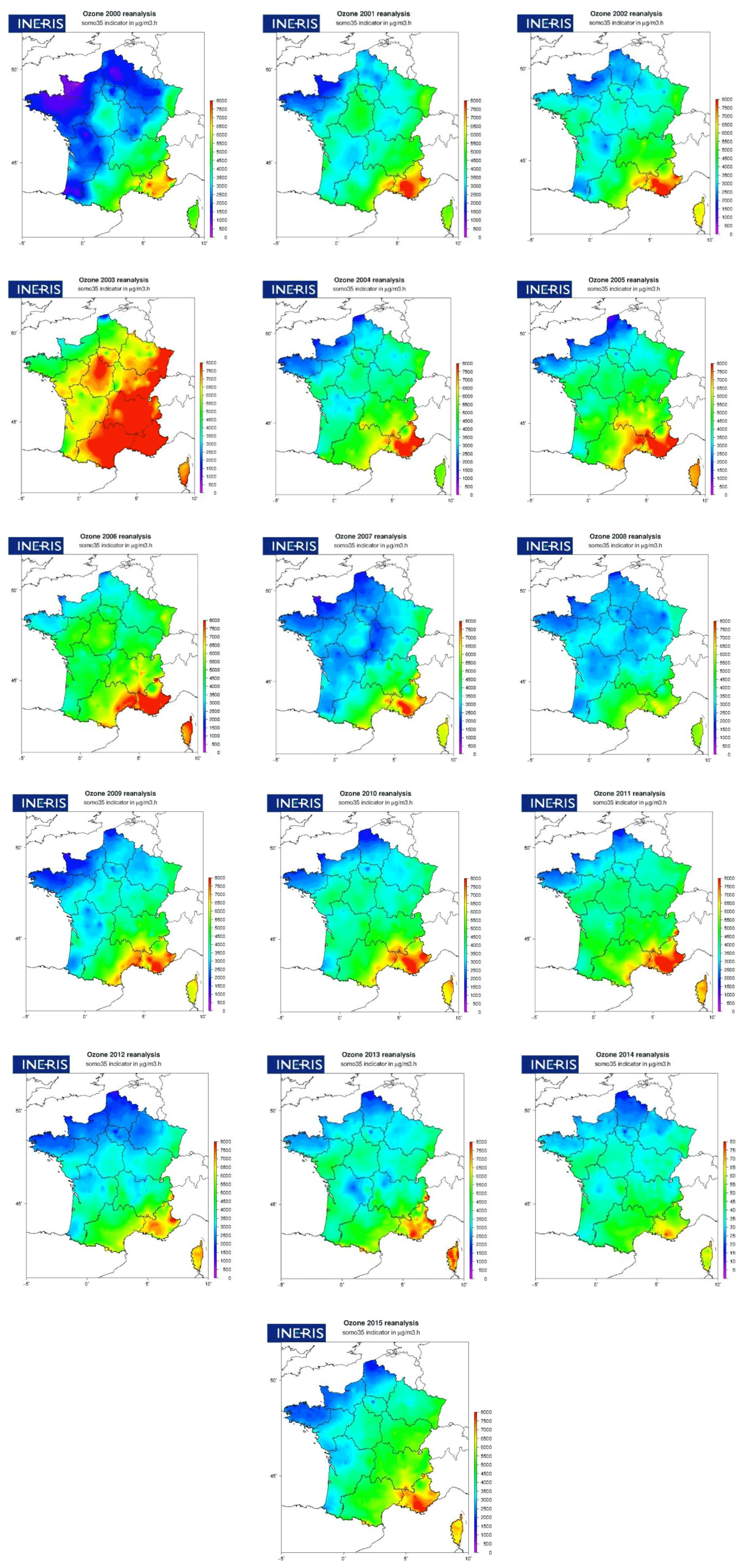
Figure 13SOMO35 indicator for the period 2000 to 2015. Ozone concentrations are obtained through a combination (kriging) of regional modeling and observations.
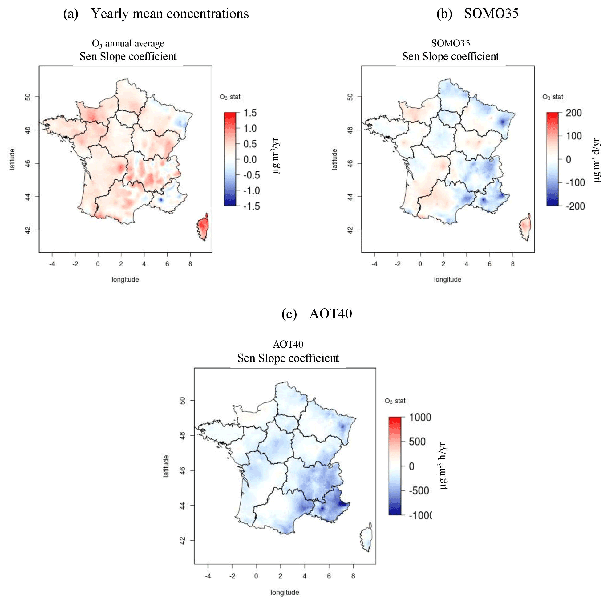
Figure 14Trends in annual mean O3 concentrations (in µg m−3 yr−1) (a), as well as SOMO35 (in µg m−3 d−1 yr−1) (b) and AOT40 (in µg m−3 h−1 yr−1) (c) indicators. Sen slope are calculated over the period 2000–2015.
3.4 NO2
Rural scores for NO2 are worse for particles and O3. The correlations are between 0.55 and 0.7, but above all, strong positive biases are observed for all years with an overestimation of the observations of 60 % to 80 %. This also affects RMSE scores that can exceed 100 % of the annual mean concentration. This poor performance can be explained by the strong spatial gradients in NO2 concentrations due to its shorter atmospheric lifetime than O3 or particles. There are too few rural stations to properly capture this variability in the kriging technique used here, so the urban stations have too much weight, and the raw model concentrations also overestimate rural concentrations.
The urban scores for NO2 are much better than the rural scores. The correlations are around 0.8, the biases do not exceed −3.5 %, and the RMSE is between 10 and 12 µg m−3 (less than 25 % of the annual mean concentration). The high number of urban background stations seems satisfactory to allow the kriging technique to correctly reproduce the spatial variability in NO2 in urban background environments. It should be noted, however, that traffic stations are not used in the present analysis (whether as observational data to be compared with or included in kriging).
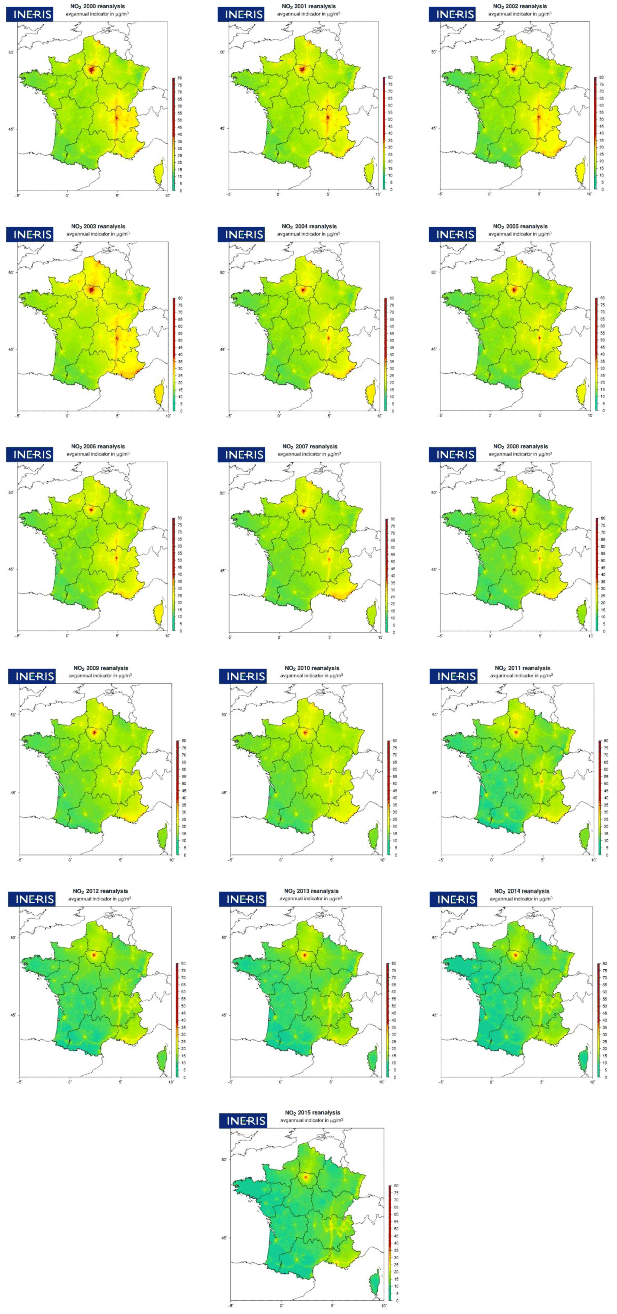
Figure 15NO2 annual mean concentrations for the period 2000 to 2015. NO2 concentrations are obtained through a combination of regional modeling and observations.
3.5 Comparison with other scores
In order to evaluate the added value of the kriging technique compared to the raw CHIMERE model simulations, the cross-validation scores can be compared to the raw model scores. Table 3 shows the scores averaged over all years and all observations without distinction of typology.
Table 3Validation scores for the raw data and the kriged concentrations (cross-validation). Annual scores (bias, RMSE and the Pearson correlation coefficient r2) are calculated over France for all years and all stations and are averaged.
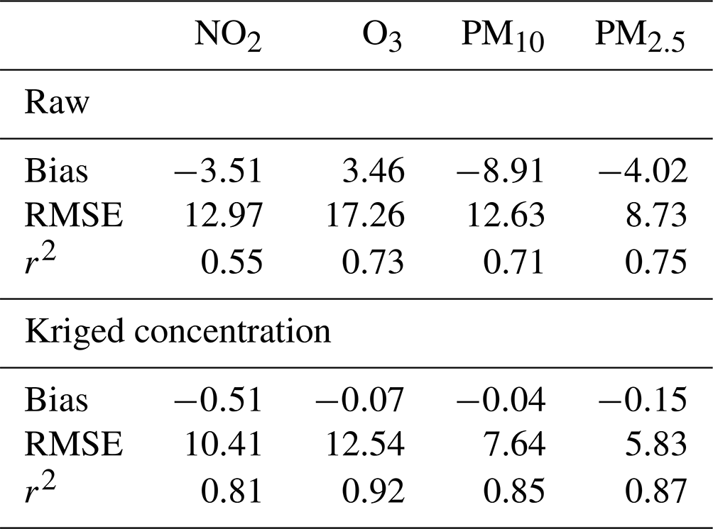
All scores are strongly improved by the kriging method of observations with CHIMERE in external drift. However, as can be seen in the previous figures, this improvement is more pronounced in urban areas than in rural areas due to the much larger number of stations in urban areas, which makes the kriging more representative of these areas.
The cross-validation scores can also be compared with those obtained in Europe with other mapping methods. Chen et al. (2019) compared 16 algorithms to develop Europe-wide spatial models of PM2.5 and NO2, included linear stepwise regression, regularization techniques and machine learning methods. Those models were developed based on the 2010 routine monitoring data from the Airbase dataset, satellite observations, dispersion model estimates and land-use variables as predictors. De Hoogh et al. (2018) also performed cross-validation of their fine-spatial-scale land-use regression models (also based on Airbase dataset, satellite observations, dispersion model estimates and land-use variables as predictors) used in Europe for the year 2010. Results from their cross-validation are compared to our own cross-validation results in Table 4.
The comparison of performance in these three studies is of course limited by the fact that the spatial coverage differs: in De Hoogh et al. (2018) and Chen et al. (2019), the cross-validation is computed over the whole of Europe. In this study, the performances are assessed over France.
For all pollutants the spatial correlation (r2) is better in our study. At the same time, higher RMSEs are also found for our study. This may be due to a larger bias, but we also demonstrated in our paper that the bias was very small, except at rural NO2 stations. Since the RMSE score also depends on the absolute concentrations, the different spatial coverage may also play a role. The lower RMSE over Europe could be an artifact of including areas where absolute concentrations of NO2, PM2.5 or O3 are lower than over France.
The validation scores obtained, as well as the comparison with raw data and with other mapping methods, allow us to be confident about the validity of the concentrations obtained and their good representativeness of background concentrations, in particular in urban areas. A crucial step appears, however, when it comes to the representativeness of rural NO2 concentrations which are overestimated in our results.
After ensuring the validation of the kriged concentration data, yearly indicators, trend over years and human exposition are calculated. Hourly concentrations fields are produced from 2000 to 2015 for NO2, O3 and PM10; however, as explained in Sect. 2, for PM10 only annual mean indicator maps are produced before 2007. PM2.5 hourly concentrations are calculated for the years 2009 to 2015 due to the limited number of background stations available before 2009.
4.1 Concentration maps and trends
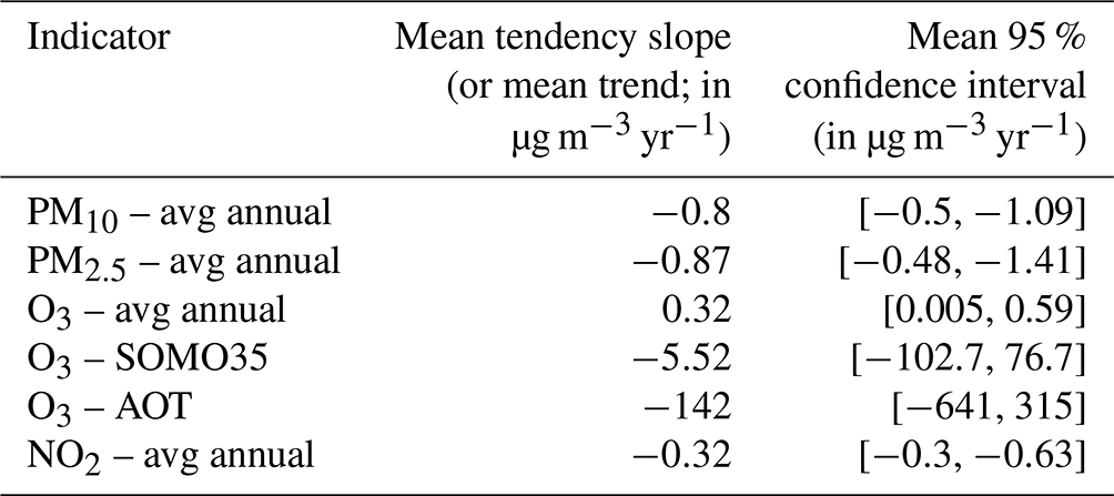
All the indicators presented in Sect. 2 are calculated, but the following sections focus on the annual averaged concentrations of PM10, PM2.5, NO2 and O3, as well as SOMO35 and AOT (two indicators associated with O3), for which mapped data are presented. These indicators are presented in this paper and available on a Zenodo repository and on an online map library (see Sect. 5). A total of 34 trend analyses over the period are performed by calculating the Sen–Theil regression slope for each grid point on the domain. To characterize the significance of these trend slopes, the 95 % confidence interval is calculated. This confidence interval represents the lower and upper values above or below which there is 95 % confidence that the trends will occur. The smaller the confidence interval is, the more statistically significant the trend will be. Large confidence intervals are considered as unrepresentative, especially those containing 0. Trend slopes and confidence intervals are calculated for each grid point in the domain, and country-averaged values are also given in Table 5.
4.1.1 PM10
Maps of annual average PM10 concentration maps are presented in Fig. 9 for the period 2000–2015. The resolution of the grid (around 4 km) allows us to see patterns such as interconnected cities, especially in the latest years during which the patterns of large inter-regional concentrations are decreasing. The impact of meteorological conditions is also visible through the interannual variability. For example, the 2003 heat wave year is associated with higher PM10 levels due to the increased formation of secondary aerosols.
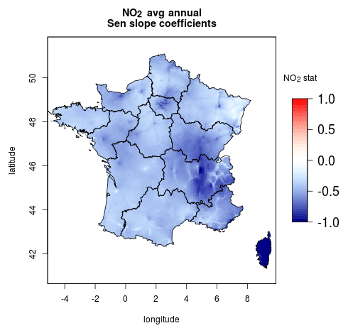
Figure 16Trends in yearly mean NO2 concentrations. Sen slope coefficients (µg m−3 yr−1) are calculated over the period 2000–2015.
Figure 10 shows the mapped trends in annual average PM10 expressed as Sen–Theil regression slope in micrograms per cubic meter per year and calculated over the period 2000–2015.
There is a downward trend in PM10 annual mean concentrations everywhere in France and in particular in the regions with the highest PM10 concentrations at the beginning of the period: the south of France (east and west), the Auvergne–Rhône–Alpes region, the east (Grand Est) and the extreme north of France. A country-averaged downward trend in PM10 concentrations of −0.8 µg m−3 per year is estimated over the period 2000–2015 (spatial average of the trends calculated on each grid point). This trend is statistically significant on average over France with a narrow 95 % confidence interval – [−0.50, −1.09] – that does not include zero (see Table 5) and applies to almost all grid points (maps of confidence interval not shown here). Taking the year 2000 as the base year, this amounts to a 39 % reduction. In a study conducted for France over the period 2000–2010, Malherbe et al. (2017) estimated a downward trend that was twice as small (0.4). This reflects the accelerated decline in concentrations in France in recent years.
This significant downward trend is the result of the decrease in primary pollutant emissions over these 16 years in response to emission reduction measures. From 2000 to 2015, primary PM10 emissions over France were reduced by 39 %, as well as emissions of PM10 precursors such as NOx emissions (−56 %) and SOx emissions (−87 %) (data calculated by CITEPA (Interprofessional Technical Centre for Studies on Air Pollution) and extracted from the 2015 French national air quality report: https://www.statistiques.developpement-durable.gouv.fr/sites/default/files/2018-10/datalab-bilan-de-la-qualite-de-l-air-en-france-en-2015-octobre-2016-c.pdf, last access: 19 May 2022).
4.1.2 PM2.5
The highest PM2.5 values are observed at the beginning of the period and are more concentrated in the main source regions than PM10. Significant reductions in annual average background concentrations are observed over the years. The Sen slope coefficients calculated for the annual average PM2.5 (Fig. 12) over the period show negative trends over the whole territory and more pronounced ones over the southeast region, the Auvergne–Rhône–Alpes region, northern France and Brittany. A downward trend of −0.87 µg m−3 per year from a national average is calculated, again with statistical significance (95 % interval of [−0.48, −1.41] which does not contain zero). Taking 2009 as a reference year, this amounts to a 35 % decrease in 7 years. As for PM10, this negative trend is associated with the reduction in primary PM2.5 emissions and in PM2.5 precursor emissions (SOx, NOx and volatile organic compounds (VOCs)).
4.1.3 Ozone
The SOMO35 indicator shows strong interannual variability. O3 is a photochemical pollutant produced by secondary reactions in the presence of NOx, VOCs and sunlight. The hot year 2003 is distinguished by a very high SOMO35 over almost the entire territory. For each year, the highest SOMO35 is found in southeastern France and to a lesser extent in the Alsace region. The trends in SOMO35, annual average O3 and AOT40 over the years are shown in Fig. 14 for the period 2000–2015.
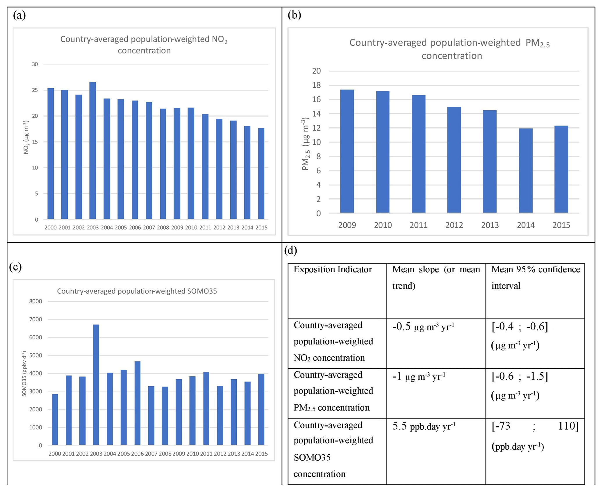
Figure 17Yearly evolution of the country-averaged population-weighted (a) NO2 concentration, (b) PM2.5 concentration and (c) SOMO35. Trends and 95 % confidence intervals are calculated (d).
For the O3 average annual concentration, small positive trends are found over France. Two exceptions are the southeast (Provence–Alpes–Côte d'Azur, or PACA, region) and the Grand Est region (east of France), i.e., the regions with the highest O3 concentrations, showing negative trends. Averaging over France, this leads to a positive trend of 0.32 µg m−3 yr−1 which corresponds to an increase of 6.5 % over 16 years. The same order of magnitude was found for the period 2000–2010 by Malherbe et al. (2017). Both negative (in the south of France) and positive trends are significant according to the mapped 95 % confidence interval (not shown). SOMO35 and AOT40 indicators, which are indicators with a threshold value below which concentrations are not taken into account, show mostly negative trends. However, according to the value of the mapped 95 % confidence interval (not shown here) on most grid points, the confidence interval is wide and contains zero, indicating a lack of significance of the calculated trends. These results are consistent with other European studies (EMEP, 2016; Malherbe et al., 2017) that show an increase in background concentrations and a decrease in O3 peaks.
Table 4Validation scores for De Hoogh et al. (2018), Chen et al. (2019), and this study. The following scores are calculated by cross-validation for the three studies: Pearson correlation coefficient r2, the bias, and the root mean square error (RMSE).
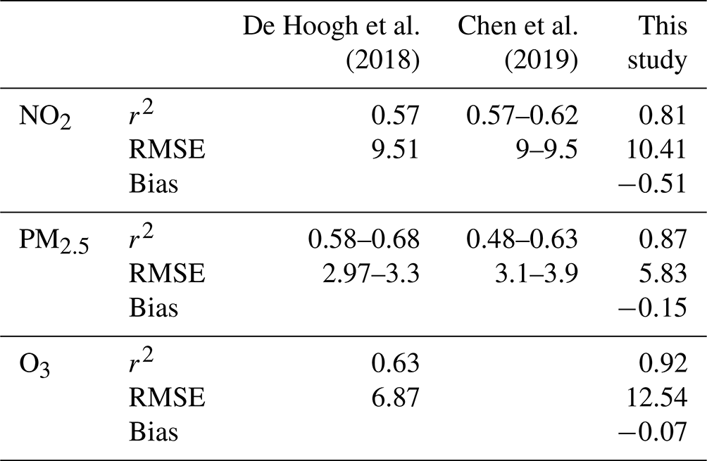
Table 5Country-averaged slope and its 95 % confidence interval.
4.1.4 NO2
NO2 is mainly emitted by road transport. All maps show the same pattern, with cities and interconnected major roads showing the highest NO2 concentrations. Trends over the period 2000–2015 are shown in Fig. 15. Decreases in NO2 concentrations are observed in both rural and urban areas throughout the country. However, we recall that rural levels were found to be overestimated with our approach (see Sect. 3.4). The decrease is more important when NO2 concentrations are high. As with PM2.5, these results highlight the combined benefit of large-scale emission management policies that target emission sectors and locally oriented policies.
On average, a significant negative trend of −0.46 µg m−3 is calculated over France with a narrow 95 % confidence interval (see Table 3). This downward trend is slightly stronger than that calculated in Malherbe et al. (2017) over the period 2000–2010 over France (−0.37 µg m−3 yr−1) and corresponds to a reduction of about 30 % (taking 2020 as the base year).
4.2 Exposure trends
Population-weighted annual average concentrations are good estimates of population exposure as they give more weight to the air pollution where people mainly live. Here, the country-averaged population-weighted concentrations of NO2, PM2.5 and SOMO35, which are the three main indicators used to calculate health impacts, are calculated for each year from the hourly kriged mapped data over France. For one pollutant, it is obtained by adding the result of multiplying the concentration by the population on all the country's grids and then dividing by the total population of the country. The population database used in this study is the LCSQA (L'expertise au service de la qualité de l'air) national population database (Létinois et al., 2014) established for the year 2015. It is based on detailed files from the French Ministry of Finance with information at building level. It is important to note that the French population used here has not varied over the years. The French population increased by about 10 % between 2000 and 2015. However, if we considered that the demographic evolution is homogeneous over the country (the urbanrural ratio has only increased by about 2.5 % in France over the same period), the population-weighted concentration on national average should be the same whatever the year of the population database.
As for the concentrations, a very clear downward trend is observed for population-weighted NO2 with a trend of −0.5 µg m−3 yr−1 and a narrow 95 % confidence interval: [−0.4, −0.6], i.e., a reduction of about 30 % in 16 years. A downward trend of −1 µg m−3 yr−1 is also clearly calculated for PM2.5 (95 % confidence interval: [−0.6, −1.5]) over the period 2009–2015, i.e., a reduction of about 31 % in 7 years. In contrast, there is no clear trend for the SOMO35 indicator over the period 2000–2015.
When the abovementioned indicators are multiplied by the total population (to obtain the total exposure, i.e., the sum of the population-weighted concentrations over a country), the outcome indicators are those used to calculate the health impact assessment based on dose-response functions, as suggested by the WHO review “Health Risks of Air Pollution in Europe”, described in Holland (2014a, b). Exposure to SOMO35, anthropic PM2.5 and NO2 (with or without threshold depending on the health impact indicator) contributes to both morbidity and mortality impacts. For example in France, they were used in the PREPA (National Air Pollutant Emissions Reduction Plan) evaluation study for which about 50 political measures to be implemented in France were evaluated and ranked on different criteria, such as air quality impact, health impact and cost–benefit assessment (Schucht et al., 2018). At constant population evolution, the trends are similar between both indicators (total exposure and population-weighted average concentration). However, the evolution in population (even if it is homogeneous over the territory) has an impact on the total exposure of the population. Therefore, we expected a reduced impact on health compared to those on population-weighted concentrations.
Mapped regulatory indicators and exposure data for all 15 years and the four pollutants described here are available on a Zenodo repository in the Netcdf format (version no. 4) and csv format for data at the municipal or regional level. The DOI link for the dataset is https://doi.org/10.5281/zenodo.5043645 (Real et al., 2021). It is also available through a web-based map library (https://www.ineris.fr/fr/recherche-appui/risques-chroniques/mesure-prevision-qualite-air/20-ans-evolution-qualite-air, Real et al., 2021). The web-based map library is intended to be updated annually. Those data have been provided to several research teams with different fields of expertise ranging from epidemiology to environmental economics and atmospheric science. Most of this work is still in progress, but other papers on the subject have been submitted or are being submitted (Favet et al., 2020; Mink, 2022; Cantrell and Michoud, 2022).
A 16-year datasets of mapped air pollution concentrations and indicators over France was constructed using a data fusion technique (kriging) that combines measurements from background surface monitoring stations and modeling from the regional model CHIMERE. The resulting data are hourly concentrations at a resolution of about 4 km over France for the period 2000–2015 (shorter period for PM2.5 and PM10 hourly indicators).
The kriging technique implemented combines kriging with external drift for NO2 and O3 and co-kriging with external drift for particulate matter, allowing the PM2.5 estimation to benefit from the highest density of PM10 monitoring stations. These datasets have been evaluated over several years using a cross-validation process that takes into account the incorporation of measurements in the correction process by retaining a data point before calculating the score. The kriging technique significantly improves the validation scores, especially in urban areas with very low biases and high correlations. However, a crucial point appears concerning the representativeness of NO2 concentrations in rural areas which are overestimated by the model. A new methodology is being developed to better map NO2 concentrations in these rural areas. It should be noted that the performance increases with the number of measurements taken into account until a threshold is reached at which the addition of stations no longer seems to improve performance. This threshold depends on the pollutant and is higher for pollutants with a strong spatial gradient (i.e., NO2 which has a shorter lifetime).
The main annual indicators (mean NO2, PM10, PM2.5, O3, SOMO35 and AOT40) are analyzed in this article, and the annual trends are calculated. Significant downward trends are calculated over the whole period for annual average concentrations of PM10, PM2.5 and NO2. They reflect the reductions in precursor emissions that have taken place in Europe since the 1990s. The trends for O3 over the 16 years are less significant. In general, the background O3 level is increasing, mainly due to large-scale pollution, and high (peaks) O3 levels are decreasing due to reductions in local O3 precursor emissions. This results in a positive trend for the annual average O3 concentration over most of France, but a small downward trend is also observed in the regions with the highest O3 levels (southeast and east). No significant trend is calculated for the two O3 indicators detailed here (SOMO35 and AOT40). Population exposure is also calculated over France. The average weight of NO2 and PM2.5 in the population of the country decreases respectively by 30 % in 16 years and 31 % in 7 years. No clear trend was found for the population weight of SOMO35.
Data kriging, results evaluation by cross-validation process, and maps and graph production for the paper were performed by ER. The CHIMERE modeling concentration data over the period 2000–2015 were produced by FC. Software developments for the kriging and cross-validation methods were provided by AU, LM and AG. The web-based map library used to store and visualize the data was developed by BR. All work has been supervised and conceptualized by AC. The manuscript draft was mainly written by ER with contributions from all co-authors.
The contact author has declared that neither they nor their co-authors have any competing interests.
Publisher's note: Copernicus Publications remains neutral with regard to jurisdictional claims in published maps and institutional affiliations.
This work was supported by the French ministry in charge of ecology. Part of the simulations was carried out in the XENAIR project funded by the ARC Foundation for Cancer Research.
This research has been supported by the Ministère de l'Écologie, du Développement Durable et de l'Énergie (grant no. program DRC16).
This paper was edited by Bo Zheng and reviewed by two anonymous referees.
Amann, M., Bertok, I., Borken-Kleefeld, J., Cofala, J., Heyes, C., Höglund-Isaksson, L., Klimont, Z., Nguyen, B., Posch, M., Rafaj, P., Sandler, R., Schöpp, W., Wagner, F., and Winiwarter, W.: Cost-effective control of air quality and greenhouse gases in Europe: Modeling and policy applications, Environ. Modell. Softw., 26, 1489–1501, 2011.
Beelen, R., Hoek, G., Pebesma, E., Vienneau, D., de Hoogh, K., and Briggs, D. J.: Mapping of background air pollution at a fine spatial scale across the European Union, Sci. Total Environ., 407, 1852–1867, 2009.
Beauchamp, M.: LCSQA notes, https://www.lcsqa.org/system/files/media/documents/lcsqa2015-note_cartes_analysees-drc-16-152350-11840a_0.pdf (last access: 19 May 2022), 2015.
Beauchamp, M., de Fouquet, C., and Malherbe, L.: Dealing with non-stationarity through explanatory variables in kriging-based air quality maps, Spatial statistics, 22, 18–46, https://doi.org/10.1016/j.spasta.2017.08.003, 2017.
Benmerad, M., Slama, R., Botturi, K., Claustre, J., Roux, A., Sage, E., Reynaud-Gaubert, M., Gomez, M., Kessler, R., Brugière, O., Mornex, J.-F., Mussot, S., Dahan, M., Boussaud, V., Danner-Boucher, I., Dromer, C., Knoop, C., Auffray, A., Lepeule, J., Malherbe, L., Meleux, F., Nicod, L., Magnan, A., Pison, C., and Siroux, V.: Chronic effects of air pollution on lung function after lung transplantation in the Systems prediction of Chronic Lung Allograft Dysfunction (SysCLAD) study, Euro. Respir. J., 49, 1600206, https://doi.org/10.1183/13993003.00206-2016, 2017.
Bentayeb, M., Stempfelet, M., Wagner, V., Zins, M., Bonenfant, S., Songeur, C., Sanchez, O., Rosso, A., Brulfert, G., Rios, I., Chaxel, E., Virga, J., Armengaud, A., Rossello, P., Rivière, E., Bernard, M., Vasbien, F., and Deprost, R.: Retrospective modeling outdoor air pollution at a fine spatial scale in France, 1989–2008, Atmos. Environ., 92, 267–279, 2014.
Bessagnet, B., Malherbe, L., and Aymoz, G. : Bilan de la première année de mesure des PM10 ajustées en France et évaluation des outils de modélisation, Rapport LCSQA, https://www.lcsqa.org/system/files/media/documents/DRC_08_94306_15151A_Bilan_PM10_corrige_vf.pdf (last access : 22 May 2022), 2008.
Briggs, D. J., de Hoogh, C., Gulliver, J., Wills, J., Elliott, P., Kingham, S., and Smallbone, K.: A regression-based method for mapping traffic-related air pollution: application and testing in four contrasting urban environments, Sci. Total Environ., 253, 151–167, 2000.
Cantrell, C., Michoud, V., Formenti, P., Doussin, J.-F., Alhajj Moussa, S., Cirtog, M., Gratien, A., and Picquet-Varrault, B. and the ACROSS Team: A Future Multi-Platform Atmospheric Chemistry Measurement Campaign to Study Oxidation in Mixed Anthropogenic-Biogenic Air Masses, EGU General Assembly 2021, online, 19–30 Apr 2021, EGU21-15448, https://doi.org/10.5194/egusphere-egu21-15448, 2021.
Chen, J., de Hoogh, K., Gulliver, J., Hoffmann, B., Hertel, O., Ketzel, M., Bauwelinck, M., Donkelaar, A., Hvidtfeldt, H. A., Katsouyanni, K., Janssen, N. A. H., Martin, R. V., Samoli, E., Schwartz, P. E., Stafoggia, M., Bellander, T., Strak, M., Wolf, K., Vienneau, D., Vermeulen, R., Brunekreef, B., and Hoek, G.: A comparison of linear regression, regularization, and machine learning algorithms to develop Europe-wide spatial models of fine particles and nitrogen dioxide, Environ. Int., 130, 104934, https://doi.org/10.1016/j.envint.2019.104934, 2019.
Chiles, J.-P. and Delfiner, P. P.: Geostatistics: Modeling Spatial Uncertainty, Vol. 497, John Wiley & Sons, 726 pp., 2012.
Colette, A., Andersson, C., Manders, A., Mar, K., Mircea, M., Pay, M.-T., Raffort, V., Tsyro, S., Cuvelier, C., Adani, M., Bessagnet, B., Bergström, R., Briganti, G., Butler, T., Cappelletti, A., Couvidat, F., D'Isidoro, M., Doumbia, T., Fagerli, H., Granier, C., Heyes, C., Klimont, Z., Ojha, N., Otero, N., Schaap, M., Sindelarova, K., Stegehuis, A. I., Roustan, Y., Vautard, R., van Meijgaard, E., Vivanco, M. G., and Wind, P.: EURODELTA-Trends, a multi-model experiment of air quality hindcast in Europe over 1990–2010, Geosci. Model Dev., 10, 3255–3276, https://doi.org/10.5194/gmd-10-3255-2017, 2017.
Couvidat, F., Bessagnet, B., Garcia-Vivanco, M., Real, E., Menut, L., and Colette, A.: Development of an inorganic and organic aerosol model (CHIMERE 2017β v1.0): seasonal and spatial evaluation over Europe, Geosci. Model Dev., 11, 165–194, https://doi.org/10.5194/gmd-11-165-2018, 2018.
De Fouquet, C., Gallois, D., and Perron, G.: Geostatistical characterization of the nitrogen dioxide concentration in an urban area : Part I : Spatial variability and cartography of the annual concentration, Atmos. Environ., 41, 6701–6714, 2007.
De Hoogh, K., Chen, J., Gulliver, J., Hoffmann, B., Hertel, O., Ketzel, M., Bauwelinck, M., Donkelaar, A., Hvidtfeldt, U. A., Katsouyanni, K., Klompmaker, J., Martin, R. V., Samoli, E., Schwartz, P. E., Stafoggia, M., Bellander, T., Strak, M., Wolf, K., Vienneau, D., Brunekreef, B., and Hoek, G.: Spatial PM2.5, NO2, O3 and BC models for Western Europe–Evaluation of spatiotemporal stability, Environ. Int., 120, 81–92, 2018.
Denier van der Gon, H. A. C., Bergström, R., Fountoukis, C., Johansson, C., Pandis, S. N., Simpson, D., and Visschedijk, A. J. H.: Particulate emissions from residential wood combustion in Europe – revised estimates and an evaluation, Atmos. Chem. Phys., 15, 6503–6519, https://doi.org/10.5194/acp-15-6503-2015, 2015.
European Environment Agency (EEA): Air Quality in Europe – 2018 Report, Copenhagen, Report No. 12/2018, 2018.
EMEP: Air pollution trends in the EMEP region between 1990 and 2012, joint report of TFMM/CCC/MSC-E and MSC-W, European Monitoring and Evaluation Programme, Norway, CCC-Report 1/2016, http://www.nilu.no/projects/ccc/reports/cccr1-2016.pdf (last access: 19 July 2019), 2016.
Fayet, Y., Praud, D., Fervers, B., Ray-Coquard, I., Blay, J.-Y., Ducimetiere, F., Fagherazzi, G., and Faure, E.: Beyond the map: evidencing the spatial dimension of health inequalities, Int. J. Health. Geogr., 19, 1–11, https://doi.org/10.1186/s12942-020-00242-0, 2020.
Goovaerts, P. (Eds.): Geostatistics for Natural Resources Evaluation, Oxford University Press, New York, 483 pp., 1997.
Holland, M.: Implementation of the HRAPIE Recommendations for European Air Pollution CBA work, Health Impact Assessment and Cost Benefit Analysis, EMRC, https://ec.europa.eu/environment/air/pdf/CBA%20HRAPIE%20implement.pdf (last access: 19 May 2022), 2014a.
Holland, M.: Cost-benefit Analysis of Final Policy Scenarios for the EU Clean Air Package, Version 2, Corresponding to IIASA TSAP Report 11, Version 1, EMRC, https://ec.europa.eu/environment/air/pdf/TSAP%20CBA.pdf (last access: 19 May 2022), 2014b.
Honoré, C., Menut, L., Bessagnet, B., Meleux, F., Rouïl, L., Vautard, R., Poisson, N., and Peuch, V. H.: PREV'AIR: A platform for air quality monitoring and forecasting, Chapter 3.4, Dev. Environm. Sci., 6, 293–300, 2007.
Horálek, J., de Smet, P., Corbet, L., Kurfürst, P., and de Leeuw, F.: European air quality maps of PM and ozone for 2010 and their uncertainty, ETC/ACM Technical Paper 2012/12, 74 pp., 2012.
Horálek, J., de Smet, P., de Leeuw, F., Kurfürst, P. and Benešová, N.: European air quality maps for 2015, ETC/ACM Technical Paper, vol. 7., 2017.
Horálek, J., Schreiberova, M., Vlasakova, L., Markova, J., Tognet, F., Schneider, P., Kurfürst, P., and Schovankova, J.: European air quality maps for 2018, Eionet Report, ETC/ATNI 2020/10, 2020.
Institute for Health Metrics and Evaluation (IHME): The Global Burden of Disease: Generating Evidence, Guiding Policy – European Union and European Free Trade Association Regional Edition, Seattle, WA, IHME, https://www.healthdata.org/policy-report/global-burden-disease-generating-evidence-guiding-policy (last access: 20 May 2022), 2013.
Janssen, S. and Thunis, P.: FAIRMODE Guidance Document on Modelling Quality Objectives and Benchmarking, version 3.2, Publications Office of the European Union, Luxembourg, EUR 30264 EN, JRC120649, 54 pp., https://doi.org/10.2760/30226, 2020.
Létinois, L.: Méthodologie de répartition spatiale de la population, LCSQA report, https://www.lcsqa.org/system/files/media/documents/drc-15-144366-00427a_modelisation_methodologie_population_2014_vf.pdf (last access: 19 May 2022), 2014.
Lichternstern, A.: Kriging methods in spatial statistics, BA thesis, Technische Universität München, Department of Mathematics, https://mediatum.ub.tum.de/doc/1173364/file.pdf (last access: 19 May 2022), 2013.
Mailler, S., Menut, L., Khvorostyanov, D., Valari, M., Couvidat, F., Siour, G., Turquety, S., Briant, R., Tuccella, P., Bessagnet, B., Colette, A., Létinois, L., Markakis, K., and Meleux, F.: CHIMERE-2017: from urban to hemispheric chemistry-transport modeling, Geosci. Model Dev., 10, 2397–2423, https://doi.org/10.5194/gmd-10-2397-2017, 2017.
Malherbe, L. and Ung, A.: Travaux relatifs à la plate-forme nationale de modélisation PREV'AIR: Réalisation de cartes analysées d'ozone (2/2), rapport LCSQA, https://www.lcsqa.org/system/files/media/documents/drc-10-103351-01139a_prevair-2_vf.pdf (last access: 19 May 2022), 2009.
Malherbe, L., Beauchamp, M., Bourin, A, and Sauvage, S.: Analyse de tendances nationales en matière de qualité de l'air, Rapport final LCSQA, , https://www.lcsqa.org/system/files/media/documents/lcsqa2016-tendances_nationales_qa_vf.pdf (last access: 19 May 2022), 2017.
Marécal, V., Peuch, V.-H., Andersson, C., Andersson, S., Arteta, J., Beekmann, M., Benedictow, A., Bergström, R., Bessagnet, B., Cansado, A., Chéroux, F., Colette, A., Coman, A., Curier, R. L., Denier van der Gon, H. A. C., Drouin, A., Elbern, H., Emili, E., Engelen, R. J., Eskes, H. J., Foret, G., Friese, E., Gauss, M., Giannaros, C., Guth, J., Joly, M., Jaumouillé, E., Josse, B., Kadygrov, N., Kaiser, J. W., Krajsek, K., Kuenen, J., Kumar, U., Liora, N., Lopez, E., Malherbe, L., Martinez, I., Melas, D., Meleux, F., Menut, L., Moinat, P., Morales, T., Parmentier, J., Piacentini, A., Plu, M., Poupkou, A., Queguiner, S., Robertson, L., Rouïl, L., Schaap, M., Segers, A., Sofiev, M., Tarasson, L., Thomas, M., Timmermans, R., Valdebenito, Á., van Velthoven, P., van Versendaal, R., Vira, J., and Ung, A.: A regional air quality forecasting system over Europe: the MACC-II daily ensemble production, Geosci. Model Dev., 8, 2777–2813, https://doi.org/10.5194/gmd-8-2777-2015, 2015.
Mink, J.: Putting a price tag on air pollution: the social healthcare costs of air pollution in France, in prep, 2022.
Real, E., Couvidat, F., Ung, A., Malherbe, L., Raux, B., Gressent, A., and Colette, A.: Historical reconstruction of background air pollution over France for 2000–2015, Zenodo [data set], https://doi.org/10.5281/zenodo.5043645, 2021 (data available at: https://www.ineris.fr/fr/recherche-appui/risques-chroniques/mesure-prevision-qualite-air/20-ans-evolution-qualite-air, last access: 19 May 2022).
Riviere, E., Bernard, J., Hulin, A., Virga, J., Dugay, F., Charles, M. A., Cheminat, M., Cortinovis, J., Ducroz, F., Laborie, A., Malherbe, L., Piga, D., Real, E., Robic, P. Y., Zaros, C., Seyve, E., and Lepeule, J.: Air pollution modeling and exposure assessment during pregnancy in the French Longitudinal Study of Children (ELFE), Atmos. Environ., 205, 103–114, 2019.
Rivoirard, J. and Romary, T.: Continuity for kriging with moving neighborhood, Mathematical Geosciences, Springer Verlag, 43, 469–481 pp., 2011.
Rouïl, L., Honore, C., Vautard, R., Beekmann, M., Bessagnet, B., Malherbe, L., Beekmann, L., Bessagnet, B., Malherbe, L., Meleux, F., Dufour, A., Elichegaray, C., Flaud, J.-M., Menut, L., Martin, D., Peuch, A., Peuch, V.-H., and Poisson, N.: PREV'AIR: an operational forecasting and mapping system for air quality in Europe, B. Am. Meteorol. Soc., 90, 73–84, 2009.
Schucht, S., Real, E., Couvidat, F., Rouil, L., Brignon, J. M., Allemand, N., Le Clercq, G., and Fayolle, D.: Economic analysis of health impacts in the National Air Pollution Control Programme, Environnement, Risques & Santé, 17, 393–400, 2018.
Skamarock, W. C., Klemp, J. B., Dudhia, J., Gill, D. O., Barker, D. M., Wang, W., and Powers, J. G.: A description of the Advanced Research WRF version 3, NCAR Technical note-475+ STR, University Corporation for Atmospheric Research, https://doi.org/10.5065/D68S4MVH, 2008.
Shaddick, G., Salter, J. M., Peuch, V.-H., Ruggeri, G., Thomas, M. L., Mudu, P., Tarasova, O., Baklanov, A., and Gumy, S.: Global Air Quality: An Inter-Disciplinary Approach to Exposure Assessment for Burden of Disease Analyses, Atmosphere, 12, 48, https://doi.org/10.3390/atmos12010048, 2021.
Tarasick, D., Galbally, I. E., Cooper, O. R., Schultz, M. G., Ancellet, G., Leblanc, T., Wallington, T. J., Ziemke, J., Liu, X., Steinbacher, M., Staehelin, J., Vigouroux, C., Hannigan, J. W., García, O., Foret, G., Zanis, P., Weatherhead, E., Petropavlovskikh, I., Worden, H., Osman, M., Liu, J., Chang, K.-L., Gaudel, A., Lin, M., Granados-Muñoz, M., Thompson, A. M., Oltmans, S. J., Cuesta, J., Dufour, G., Thouret, V., Hassler, B., Trickl, T., and Neu, J. L.: Tropospheric Ozone Assessment Report: Tropospheric ozone from 1877 to 2016, observed levels, trends and uncertainties, Elem. Sci. Anth., 7, 39, https://doi.org/10.1525/elementa.376, 2019.
Wackernagel, H.: Multivariate Geostatistics, Springer Berlin Heidelberg, 387 pp., https://doi.org/10.1002/bimj.4710380409, 1996.