the Creative Commons Attribution 4.0 License.
the Creative Commons Attribution 4.0 License.
 | 13 May 2022
First SMOS Sea Surface Salinity dedicated products over the Baltic Sea
Verónica González-Gambau
Estrella Olmedo
Antonio Turiel
Cristina González-Haro
Aina García-Espriu
Justino Martínez
Pekka Alenius
Laura Tuomi
Rafael Catany
Manuel Arias
Carolina Gabarró
Nina Hoareau
Marta Umbert
Roberto Sabia
Diego Fernández
This paper presents the first Soil Moisture and Ocean Salinity (SMOS) Sea Surface Salinity (SSS) dedicated products over the Baltic Sea. The SSS retrieval from L-band brightness temperature (TB) measurements over this basin is really challenging due to important technical issues, such as the land–sea and ice–sea contamination, the high contamination by radio-frequency interference (RFI) sources, the low sensitivity of L-band TB at SSS changes in cold waters, and the poor characterization of dielectric constant models for the low SSS range in the basin. For these reasons, exploratory research in the algorithms used from the level 0 up to level 4 has been required to develop these dedicated products. This work has been performed in the framework of the European Space Agency regional initiative Baltic+ Salinity Dynamics.
Two Baltic+ SSS products have been generated for the period 2011–2019 and are freely distributed: the Level 3 (L3) product (daily generated 9 d maps in a 0.25∘ grid; https://doi.org/10.20350/digitalCSIC/13859, González-Gambau et al., 2021a) and the Level 4 (L4) product (daily maps in a 0.05∘ grid; https://doi.org/10.20350/digitalCSIC/13860, González-Gambau et al., 2021b), which are computed by applying multifractal fusion to L3 SSS with SST maps. The accuracy of L3 SSS products is typically around 0.7–0.8 psu. The L4 product has an improved spatiotemporal resolution with respect to the L3 and the accuracy is typically around 0.4 psu. Regions with the highest errors and limited coverage are located in Arkona and Bornholm basins and Gulfs of Finland and Riga.
The impact assessment of Baltic+ SSS products has shown that they can help in the understanding of salinity dynamics in the basin. They complement the temporally and spatially very sparse in situ measurements, covering data gaps in the region, and they can also be useful for the validation of numerical models, particularly in areas where in situ data are very sparse.
- Article
(2594 KB) - Full-text XML
- BibTeX
- EndNote


The Baltic Sea is a strongly stratified semi-enclosed shallow sea that has several sub-basins, which are mostly separated from each other by underwater sills. The water balance is positive with large freshwater supply from rivers and precipitation and with occasional high-saline water input from the North Sea through the narrow and shallow Danish straits. The propagation of the saline water inflows in the deeper layers is hampered by bathymetry; the basins are connected to each other through narrow channels and shallow sills and by hydrodynamic restrictions including brackish water outflow, fronts and mixing. The mean depth of the Baltic Sea is only 54 m, which yields to highly variable ocean dynamics mainly controlled by local atmospheric forcing (Leppäranta and Myrberg, 2009). The sill areas between the basins are usually shallower than the halocline depth. The bottom waters in the southern and central basins are mainly ventilated by major Baltic saltwater inflows (Matthäus and Franck, 1992; Fischer and Matthäus, 1996; Mohrholz, 2018). Therefore, the central Baltic Sea and western Gulf of Finland deep waters suffer from anoxia, which is not the case in other sub-basins. The Gulf of Bothnia and Gulf of Riga are ventilated by upper-layer waters from the central Baltic Sea. However, there is a growing concern that changes are going on and the environmental state of these areas may worsen.
The surface layer salinities in the southern and central basins are between 6.5–8.5 psu, being highest in the southern part and decreasing towards the north. Due to the voluminous river discharge the salinity decreases towards the ends of the sub-basins in the northern and eastern extremity. Salinities in the basins also differ from each other clearly. In the Bothnian Sea, the surface salinity is typically between 5–6 psu, in the Bothnian Bay between 2–4 psu and in the Gulf of Riga 4.5–6 psu. The Gulf of Finland is an exception, because it is a direct continuation of the central basin and resembles a very large estuary, having a continuous salinity gradient in the surface salinity decreasing from 6 psu in the western part close to 0 psu in the eastern part. Surface salinity is thus an indicator of the dynamics and changes in the conditions of the basins and of the exchange between them. More detailed descriptions of the salinity variation and dynamics in the Baltic Sea can be found for example in Leppäranta and Myrberg (2009) and Lehmann et al. (2022).
Complex oceanographic conditions within the Baltic Sea are a challenge for oceanographic models and, for example, the salinity dynamics cannot be comprehensively simulated by the present model systems (e.g., Meier et al., 2006; Hordoir et al., 2019; Lehmann et al., 2022). Furthermore, model simulations of the Baltic Sea are constrained by the measurements available for calibrating and validating the models, and compiling and assimilating the initial fields. Hence, additional satellite data are crucial to improve the performance of the Baltic Sea models. In situ temperature and salinity observations in the Baltic Sea have been performed from research vessels regularly since 1898. Traditionally, the countries around the Baltic Sea deliver data to the International Council for the Exploration of the Sea (ICES). The present internationally coordinated monitoring data are collected under programs of HELCOM (http://www.helcom.fi, last access: 13 November 2019), which is the governing body (since 1979, Helsinki) in the Convention on the Protection of the Marine Environment of the Baltic Sea. There are other oceanography data portals that also include Baltic Sea data (e.g., SHARK, SeaDataNet, EMODnet, Baltic Nest Institute). The contents of these data sources are largely overlapping. In general, the sampling of the in situ data is still heterogeneous in space and time.
Remote sensing has been used for decades in the Baltic Sea to follow the ice conditions, surface temperature and algal blooms. However, salinity conditions have remained outside of an overall synoptic view so far. There is a need to put in situ data in context because of the strong seasonal cycles and strong meso-scale dynamics with fronts and eddies, which have horizontal dimensions of the order of kilometers to tens of kilometers. Remotely sensed salinity information would be a valuable addition to the available tools for understanding the changes.
For all the above, Earth observation sea surface salinity (SSS) measurements have a great potential to help in the understanding of the dynamics in the basin (Omstedt et al., 2014): they can complement temporally and spatially the in situ measurements in the region, and they also can be useful for validating numerical models, especially in those areas where in situ data are sparse. Nonetheless, the Baltic Sea is one of the most challenging regions for the SSS retrieval from L-band satellite measurements. The available EO-based global SSS products over this region are quite limited, both in terms of spatiotemporal coverage and quality due to several technical limitations. In particular, the SSS retrieval from SMOS (Soil Moisture and Ocean Salinity) measurements presents the following challenges in the Baltic Sea:
-
the contamination of ocean brightness temperature (TB) measurements close to land, particularly crucial since few points are further than 110 km from the nearest coast (Martín-Neira et al., 2016);
-
the contamination of ocean TB close to ice edges, since the Bothnian Bay and the eastern part of the Gulf of Finland are ice-covered every year, and also the Baltic Proper in severe winters;
-
the high contamination by radio-frequency interference (RFI) sources (Oliva et al., 2016);
-
the low sensitivity of L-band TB to SSS changes in the cold waters (Yueh et al., 2001) of the Baltic Sea, with a typical average value of the sea surface temperature (SST) during winter of below 3 ∘C;
-
dielectric constant models that relate the TB and the SSS that were derived from salinity measurements in the range of the global ocean (32–38 psu) and are not fully tested in the low-SSS and low-SST regimes of the Baltic Sea.
For all the above conditioning factors, essential modifications have been required in the algorithms used from the very low level of processing up to the SSS retrieval to develop dedicated SSS products over the Baltic Sea:
-
In the brightness-temperature generation, the ALL-LICEF calibration approach and the correction of the correlators' efficiency errors proposed by Corbella et al. (2015) are used to mitigate the land–sea and ice–sea contamination on TB measurements.
-
In the SSS retrieval, two major changes have been introduced with respect to the original debiased non-Bayesian retrieval (Olmedo et al., 2017) used in the generation of the current global Barcelona Expert Center (BEC) SSS product (Olmedo et al., 2021b):
-
the empirical correction of the dielectric constant model for the low SSS regimes of the Baltic Sea;
-
the characterization and correction of SSS systematic errors, depending not only on the acquisition conditions, but also on the SST.
-
In this work, we present the dedicated algorithms used to develop the Baltic+ L3 and L4 SSS products and their quality assessment. The article is structured as follows: Sect. 2 describes the datasets (Sect. 2.1) and algorithms (Sect. 2.2) used in the generation of the Baltic+ SSS products. Section 3 presents the quality assessment of the SSS products. Section 3.1 presents the different datasets used for comparison and validation, Sect. 3.2 describes the methods, Sect. 3.3 explains the quality metrics used in the validation, and Sect. 3.4 shows the validation results. The conclusions are summarized in Sect. 5.
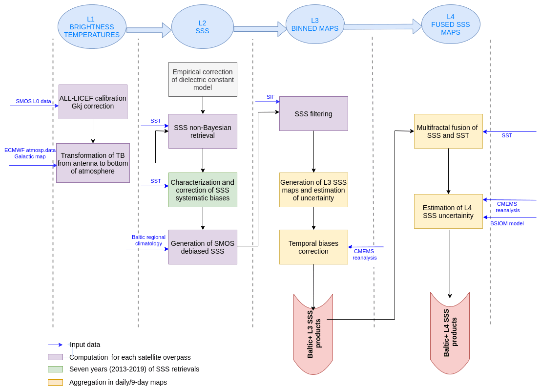
This section is devoted to explaining the datasets and the main algorithms used in the generation of the Baltic+ L3 and L4 SSS products (see Fig. 1). The processing starts from the SMOS L0 data distributed by ESA. The general algorithm encompasses several blocks (detailed in Sect. 2.2):
-
computation of brightness temperatures at antenna reference frame (ARF) from level 0 data by using the ALL-LICEF calibration and applying the Gkj correction to reduce ocean TB errors close to land and ice edges;
-
computation of the measured TB at the bottom of the atmosphere (BOA);
-
computation of the difference between SMOS TB and modeled TB and inversion to retrieve SSS;
-
correction of systematic biases on SSS by means of SMOS-based climatological data;
-
generation of the Baltic L3 salinity maps;
-
correction of temporal biases found in L3 SSS maps;
-
multifractal fusion of L3 SSS maps with an SST field to generate the L4 SSS maps.
2.1 Datasets used in the generation of the products
2.1.1 SMOS brightness temperatures
We generate the TB dataset starting from the SMOS ESA Level 0 data (https://smos-diss.eo.esa.int/oads/access/, last access: 13 November 2019). Level 0 is the raw data containing both observation data and housekeeping telemetry.
2.1.2 Auxiliary data used in the salinity retrieval
The auxiliary data used for the SSS retrieval come from the European Centre for Medium range Weather Forecast (ECMWF) (Sabater and De Rosnay, 2010). They can be accessed at https://smos-diss.eo.esa.int/oads/access/collection/AUX_Dynamic_Open (last access: 13 November 2019). ESA provides an ECMWF auxiliary file spatially and temporally collocated with each SMOS overpass. The following fields are used in the SSS retrieval: sea-ice cover, rain rate, 10 m wind speed, 10 m neutral equivalent wind (zonal and meridional components), significant wave height (SWH) of wind waves, 2 m air temperature, surface pressure and vertically integrated total water vapor (Zine et al., 2008).
We use a regional climatology as an annual reference SSS field, which is added to the debiased SMOS SSS anomalies (see Sect. 2.2.4). This regional climatology is distributed by SeaDataNet and provides temperature and salinity monthly climatologies computed from a historical dataset (mainly from CTD (conductivity, temperature and depth) devices and discrete water samplers in the period 1900–2012) (SeaDataNet Baltic Climatology, 2015), with a spatial resolution of 0.11∘ in longitude and 0.065∘ in latitude. The salinity field at 0 m depth is used. Monthly climatologies are averaged to obtain an annual reference field. A nearest-neighbor interpolation is used to compute the reference value at the grid of the debiased SMOS SSS anomalies.
2.1.3 Sea surface temperature
Since the SST is one important driver of the SSS errors, we analyzed the errors of all the available SST datasets over the Baltic sea: (i) ECMWF (Sabater and De Rosnay, 2010), (ii) OSTIA (Donlon et al., 2012), (iii) CMC (Canada Meteorological Center, 2012), (iv) REMSS (Remote Sensing Systems, 2017), (v) CCI (Merchant et al., 2019) and (vi) CMEMS Baltic Sea reanalysis (Axell, 2019). For this, we computed the differences with respect to the SeaDataNet in situ measurements (see Sect. 3.1.3). We use the SST product that provided the best performance: the ESA Sea Surface Temperature Climate Change Initiative (SST CCI) Level 4 Analysis Climate Data Record, version 2.1 (Merchant et al., 2019, https://data.ceda.ac.uk/neodc/esacci/sst/data/CDR_v2/Analysis/L4/v2.1, last access: 14 January 2020) for the period 2011–2016 and the Operational Sea Surface Temperature and Sea Ice Analysis (OSTIA) product for the period 2017–2019 (Donlon et al., 2012).
The ESA CCI SST combines data from both the Advanced Very High Resolution Radiometer (AVHRR) and Along-Track Scanning Radiometer (ATSR) SST_CCI Climate Data Records, providing daily global SST on a 0.05∘ regular latitude-longitude grid.
The OSTIA dataset uses satellite data provided by international agencies via the Group for High Resolution SST (GHRSST). These products include data from microwave and infrared satellite instruments. The OSTIA dataset also has daily global coverage on a 0.05∘ regular latitude–longitude grid.
These SST products are used in the SSS retrieval (Sect. 2.2.4), in the correction of SMOS SSS systematic biases (Sect. “Characterization and correction of SMOS SSS systematic errors”) and as a template in the fusion scheme to generate the L4 SSS product (Sect. 2.2.8).
2.1.4 Sea-ice fraction
A sea-ice mask is required to discard those SSS retrievals in ice-covered regions. This sea-ice mask is created from the sea-ice fraction (SIF) information provided by OSTIA (product ID “OSTIA-UKMO-L4-GLOB-v2.0”, Donlon et al., 2012). We generate an ice-filtering flag (SSS values are discarded when SIF >0) in order to discard those raw SSS retrievals acquired when sea ice is present.
2.1.5 CMEMS Baltic Sea reanalysis
We use the Baltic Sea physics reanalysis (CMEMS_product_ID: BALTICSEA_REANALYSIS_PHY_003_011, Axell, 2019) for the temporal correction of the Baltic+ L3 SSS maps (see Sect. 2.2.7) and for the estimation of the L4 SSS uncertainty (see Sect. 2.2.9). This product provides a 24 -year (1993–2019) reanalysis for the Baltic Sea using the ice–ocean model NEMO-Nordic and the LSEIK data assimilation scheme. Daily mean salinity at 1.5 m depth (the uppermost available salinity) is used to generate 9 d salinity fields at 0.25∘ with the same temporal coverage as the SMOS L3 SSS maps.
2.1.6 Three-dimensional coupled sea-ice–ocean model of the Baltic Sea (BSIOM)
We use the daily SSS of the BSIOM hindcast simulation using the model configuration described in Lehmann et al. (2014) with ERA5 atmospheric forcing. The horizontal resolution of the coupled sea-ice–ocean model is 2.5 km, and we use the uppermost salinity of the 60 vertical levels. These data are used for the estimation of the L4 SSS uncertainty (see Sect. 2.2.9).
2.2 Algorithm developments for Baltic+ SSS products
2.2.1 Generation of SMOS brightness temperatures
Some of the corrections we propose to improve the quality of TBs over the Baltic Sea are not included in the current operational ESA L1B products. For this reason, we have used the MIRAS Testing Software (MTS) (Corbella et al., 2008), developed by the Universitat Politècnica de Catalunya (UPC), which provides TBs at the antenna reference frame from SMOS ESA level 0 data, to generate the TB dataset.
We use the ALL-LICEF mode as the calibration approach (Corbella et al., 2016). The main advantage of using this calibration mode is that the measurements of the zero-baseline visibility, and the rest of the visibility samples, are more consistent. The up-to-date methods developed by the UPC in the recent years for reducing image reconstruction errors are also included in the MTS. Details on the image reconstruction strategy used can be found in Corbella et al. (2009, 2019).
2.2.2 Mitigation of errors in SMOS brightness temperatures
Corbella et al. (2015) showed that the dominant contribution to both land–sea contamination (LSC) and the ice–sea contamination (ISC) is caused by a mismatch between the amplitude of the zero-baseline visibility (mean antenna noise temperature) and the rest of visibilities. In particular, it was found that the error comes from an overestimation of the MIRAS correlator efficiencies (known as the Gkj parameter) and proposed a 2 % correction factor to the Gkj parameter calibrated every 2 months during the long calibration sequences (Brown et al., 2008). This corrected Gkj parameter is the one used in the denormalization of the calibrated visibilities (Corbella et al., 2005) before the TB image reconstruction.
The application of this correction leads to an overall reduction of the TB contamination close to the coasts (Corbella et al., 2015). This enhancement is also reflected globally in the quality of the SSS retrievals from the corrected TBs (González-Gambau et al., 2017).
In the Baltic, the ALL-LICEF calibration approach and the Gkj correction are crucial to reduce the LSC and ISC close to coasts and ice edges. As an indicator of the TB quality, the differences between the SMOS TB measurements and the theoretically modeled TBs at ocean surface (hereafter referred to TB anomaly) are analyzed. Details on the derivation of the modeled TBs can be found in González-Gambau et al. (2017).
The impact of the Gkj correction on the SMOS TB over the Baltic Sea is shown in Fig. 2. A significant overall reduction of the systematic biases is observed in the whole basin (∼2–3 K), improving the quality of TBs.
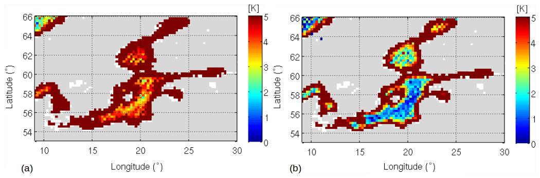
Figure 2A 9 d 0.25∘ map (June 2014) of the mean anomaly (TBSMOS−TBmod) of the first Stokes parameter divided by two, that is, the average between the horizontal and vertical polarizations of the TB () [K]. (a) TB without the Gkj correction, (b) TB after applying the Gkj correction.
González-Gambau et al. (2015) and González-Gambau et al. (2016) proposed a dedicated technique, the nodal sampling (NS), to mitigate the impact of RFI contamination. This technique has been successfully applied at a global scale (González-Gambau et al., 2017) and in the Black Sea (Olmedo et al., 2021a). However, the application of the NS for the specific case of the Baltic Sea did not show a significant improvement. In fact, this is the only basin where we did not find a positive impact when applying the NS technique. Further investigation is required to fully understand the reasons for this under-performance.
Before the salinity retrieval process, the corrected brightness temperatures are transformed from antenna to ocean surface (Olmedo et al., 2021a).
2.2.3 Empirical correction of the dielectric constant model for the Baltic Sea
The SSS retrieval is based on finding the appropriate value of raw SSS that makes the GMF (geophysical model function) of TB closer to the actually measured TB. The GMF is derived from a dielectric constant model for sea water. All the dielectric constant models found in the literature are built by empirical fitting of laboratory measurements. The dielectric constant model of Klein and Swift (1977) was used until recently in the operational SMOS L2OS (Level 2 Ocean Salinity) processor. The dielectric constant model of Meissner and Wentz (M&W) (Meissner and Wentz, 2004; Meissner et al., 2018) is used in Aquarius and SMAP salinity processors. The M&W model was reported as more suitable at low-SST ranges (Meissner and Wentz, 2004; Zhou et al., 2017). Therefore, we propose to use the M&W dielectric constant model to retrieve SSS in the Baltic Sea.
In a first analysis of the retrieved raw SSS, a low number of retrievals was obtained in some regions of the Baltic, especially in regions where the SSS values are very low. Figure 3a shows the difference between the SMOS and the modeled TB (i.e., the TB associated with the retrieved raw SSS using the GMF) for all the measurements in 2013 under the following acquisition conditions (latitude, longitude, overpass direction, across-track distance, incidence angle): , , km, . Those values for which a salinity retrieval is obtained are marked with green circles.
It was found that raw SSS values were only retrieved if TBmeas−TBmod≤0. In the Baltic Sea, the values of SSS and SST are very low and the sensitivity of SSS to TB is also very low at cold waters. Thus, large biases on TB translate to large biases on SSS, which typically leads to negative raw SSS values in the retrieval. These negative salinity values do not have any physical meaning; they just reflect the presence of instrumental biases that must be corrected.
The M&W dielectric constant model is reviewed for the SST and SSS conditions of the Baltic Sea. Figure 3b shows the modeled half first Stokes parameter as a function of the salinity for a given incidence angle (40∘) and SST (0 ∘C). The problems at low SSS values are evident: the dielectric model presents at least a maximum value for very low SSS, which causes an inversion problem for TB values that are close to this maximum (i.e., the same TB can be attributed to two different SSS values). This behavior of the models is non-physical and comes from the fact that models are constructed by polynomial fitting of experimental observations taken at the typical salinity values for the global ocean (i.e., in the range of [32–38] psu) and, therefore, the value of the dielectric constant at low SSS is an extrapolation.
For very diluted solutions, the conductivity depends almost linearly on the salinity (IOC et al., 2010). For low concentrations of salt ions (low enough to neglect interactions among ions), conductivity and emissivity depend on the amount of available ions. Thus, for low SSS, the dielectric constant should also depend almost linearly on salinity.
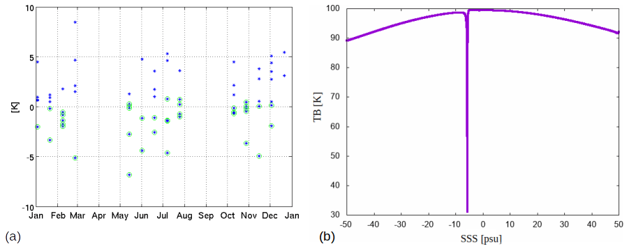
Figure 3(a) Difference of SMOS and modeled TB (blue stars) for ascending orbits in 2013 for the following acquisition conditions: (, , km, ). Green circles indicate those measurements for which a valid SSS is retrieved. (b) Half first Stokes modeled TB (M&W model) versus raw SSS for and . Note that negative SSS values do not have any physical meaning. They only reflect the presence of instrumental biases that need to be corrected.
However, as shown in Fig. 3b, the M&W model starts deviating considerably from the almost linear dependence on SSS at about 20 psu. Therefore, lacking of a better characterization of the dielectric constant at low SSS, we decided to perform a linear extension of the M&W dielectric constant model for SSS lower than 20 psu.
2.2.4 Debiased non-Bayesian SSS retrieval
The debiased non-Bayesian (DNB) SSS retrieval (Olmedo et al., 2017) focuses on the correction of the residual systematic biases in SSS (produced by LSC and permanent RFI) and on the increase in coverage with respect to the standard (Bayesian) retrieval algorithm. The original debiased non-Bayesian approach has been fine-tuned for retrieving SSS in the Baltic Sea. Major modifications are highlighted in this section.
Non-Bayesian salinity retrieval
A single SSS value is retrieved for each TB measurement at a given incidence angle, unlike the conventional Bayesian retrieval, where a single SSS is retrieved from the entire set of multi-angular TB. Details on the SSS retrieval (referred to as raw SSS, since they need to be corrected from systematic biases and filtered) can be found in Sect. 2.2 of Olmedo et al. (2017). These raw SSS data are then appropriately classified, filtered and combined, to build global SSS maps.
Characterization and correction of SMOS SSS systematic errors
We want to characterize the systematic errors in SMOS SSS. This characterization is based on the hypothesis that systematic errors are the same for all those SSS acquired under the same conditions. In total, 7 years of SMOS SSS retrievals (2013–2019, the cleanest period in terms of RFI contamination) are used for the characterization of those systematic biases on raw SSS that do not depend on time.
The raw SSS are grouped together according to their geolocation in the same fixed grid of TB measurements (coordinated by the latitude and longitude), overpass direction (ascending or descending, denoted by d), across-track distance to the center of the swath (in 50 km bins, denoted by x) and incidence angle (in 5∘ bins, denoted by θ). Then, for each group, we use the central estimator of the distribution for characterizing the systematic biases of this group. We call this central estimator the SMOS-based climatological data (see the original DNB method in Olmedo et al., 2017, for more details).
When we applied the original DNB SSS retrieval to the Baltic Sea, we observed that seasonal variations were much higher than in the global ocean (Olmedo et al., 2020) and that high gradients not corresponding to geophysical gradients (they are not observed neither in the reanalysis nor in the in situ measurements) appeared close to the coasts. These effects were evidenced when computing the monthly mean difference between the SMOS SSS and CMEMS Baltic reanalysis salinity field (Fig. 4).
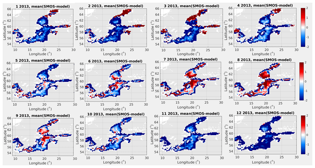
Figure 4Maps of monthly mean differences between SMOS SSS and the salinity field of CMEMS Baltic reanalysis [psu] for the year 2013.
Then, we analyzed the dependence of these differences on SST. SMOS SSS fields retrieved in 2013 were collocated with the salinity and temperature outputs from the CMEMS Baltic reanalysis. Figure 5 shows the mean of the difference between the salinity, as observed by SMOS, and the reanalysis for each bin of 1 ∘C of SST. To mitigate these systematic spatial biases dependent on SST, we modify the original DNB to include the SST (Ts) as one more parameter in the classification of the SSS retrievals for the computation of the SMOS-based climatological data.
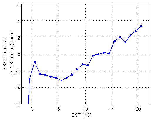
Figure 5Difference between the SMOS SSS and reanalysis salinity variability as a function of the SST.
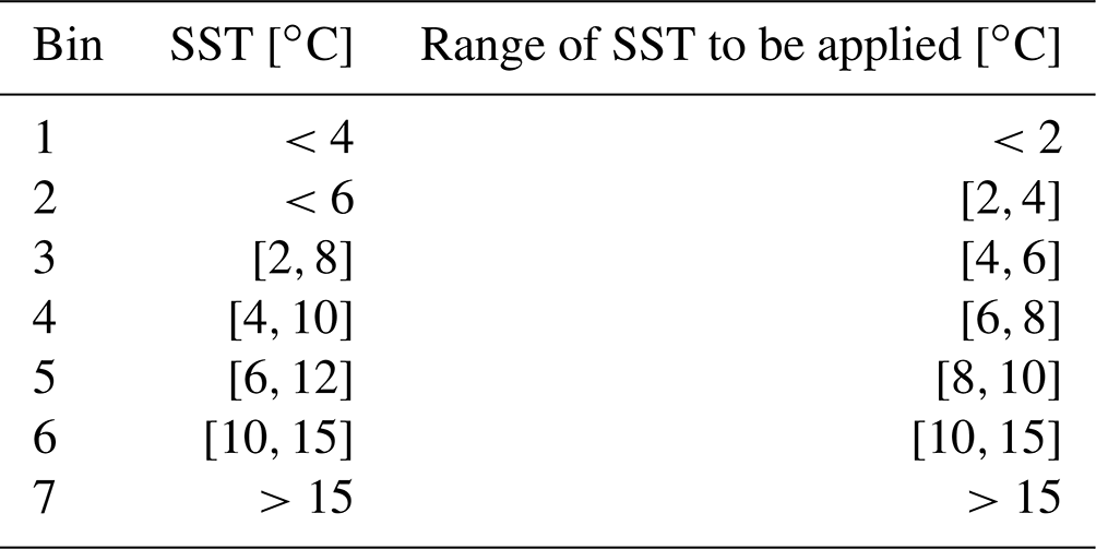
Therefore, for each given 6-tuple (instead of the 5-tuple of the original DNB), , all the raw SSS retrievals in the period 2013–2019 are accumulated. The introduction of the SST in the classification of SSS systematic errors leads to an important reduction in the number of measurements under given acquisition conditions. Therefore, to increase the number of measurements and have significant statistics, we extended the SST range when computing the SMOS-based climatological data. Seven bins of SST are defined (note that bin size varies depending on the SST range) with a certain overlap for the low ranges of SST (see Table 1).
Table 1Bins of SST for the computation of SMOS-based climatological data and the corresponding ranges of SST to be applied.
Still, the classification of the raw SSS for the 6-tuple leads to SMOS-based climatological distributions with a significantly reduced number of events. For this reason, the strategy for computing the SMOS-based climatological data, i.e., the central estimator of all the raw SSS acquired under a given 6-tuple, is changed with respect to the original DNB. We base the correction of systematic biases and filtering criteria only on the first- and second-order moments. In the Baltic Sea, the presence of outliers in the raw SSS highly impacts on the estimation of the statistical parameters that characterize the SMOS-based climatological distributions. To avoid this, the statistics are computed only with raw SSS belonging to the interval between the 5-quantile (IQ5) and the 95-quantile (IQ95). Hence, the mean (m0) and the standard deviation (σ0) of the distributions are computed in the interval [IQ5, IQ95]. Then, the SMOS-based climatological data are defined for a given acquisition condition as the averaged value of the raw SSS in the interval .
Examples of maps of the mean and the standard deviation of the SMOS-based climatological distributions are shown in Fig. 6 for two different bins of SST: bins 2 and 6 in Table 1. Note that the SMOS-based climatological values are very different for the two bins of SST and the distributions at colder temperatures are noisier, as expected, due to the low sensitivity of TB to SSS at cold waters (Yueh et al., 2001).
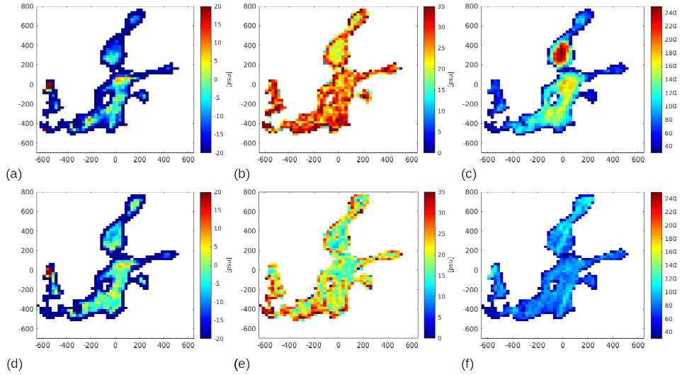
Figure 6SMOS-based climatological distributions for descending overpasses, x=0 km and . (a) Mean value for the bin 2 of SST (−10 ∘C ∘C), (b) standard deviation for the bin 2 of SST, (c) number of measurements for the bin 2 SST, (d) mean value for the bin 6 of SST (10 ∘C ∘C), (e) standard deviation for the bin 6 of SST, (f) number of measurements for the bin 6 of SST. Note that axis units are in kilometres.
Generation of debiased non-Bayesian SMOS salinities
For the generation of the debiased non-Bayesian SMOS SSS values, each raw SSS acquired at a time t and at the given acquisition condition is corrected with the corresponding SMOS-based climatological data, thus giving the SMOS-based anomalies.
Then, a time-independent SSS reference is added to the SMOS SSS anomalies to obtain the final debiased SSS values. The annual reference SSS field used is the Baltic regional climatology provided by SeaDataNet (see Sect. 2.1.2).
We study now whether the multi-annual mean of the salinity (required for the bias mitigation) changes with SST. For this, the impact of adding the regional climatology computed per bin of SST versus using a unique regional climatology as the annual reference field is analyzed. We use the salinity and temperature provided by CMEMS Baltic reanalysis in the period 2013–2019 to compute the averaged salinity for each bin of temperature. The mean error when using the single regional climatology as the annual reference field, instead of using the mean salinity value per bin of temperature (taking into account the frequency of each temperature value), is shown in Fig. 7. The typical error is around 0.05 psu, except in the Danish straits, where can reach up to 0.4 psu. Since this error is, in general, quite low in the basin, a single annual reference field is used to generate the debiased SMOS SSS.
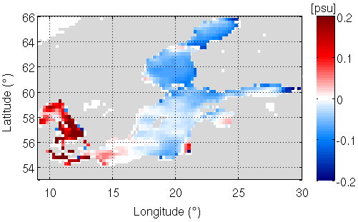
Figure 7Mean error when applying a single annual reference climatology instead of a different climatology computed for each bin of temperature.
2.2.5 Filtering criteria
Errors in SSS retrievals over the Baltic Sea are expected to be much larger than in the global ocean, due to the low sensitivity of SSS to TB at cold waters. Moreover, residual errors caused by land–sea and ice–sea contamination, as well as perturbations by RFI sources, are also affecting the salinity retrievals. For this reason, the filtering criteria defined for the BEC global product (Olmedo et al., 2021b) are not suitable for this basin. In this work, the filtering criteria are reviewed and made less restrictive while giving accurate enough values for the Baltic Sea.
The filtering criteria are the following:
-
Any raw SSS out of the range [−150, 100] psu is not considered. Note that negative values have not any physical meaning. They reflect the instrumental biases and other systematic errors that need to be corrected.
-
For a given 6-tuple, , the SMOS-based climatological distribution under at least one of these conditions is discarded:
-
The histogram has less than 30 measurements.
-
The standard deviation is greater than 35 psu.
If the SMOS-based climatological distribution corresponding to a given 6-tuple has been discarded following the previous criteria, then all the associated raw SSS are discarded.
-
-
Raw SSS are discarded if they deviate too much from the SMOS-based climatological data. That is, any raw SSS value outside the interval defined by (see Sect. “Characterization and correction of SMOS SSS systematic errors”) is discarded (see examples in Fig. 6). Note that the standard deviation of the distributions is much higher than the expected geophysical variability of SSS. Therefore, this criterion is not very restrictive.
-
In order to improve the quality of L3 SSS maps, all SSS values with an associated SSS uncertainty (estimated as detailed in Sect. 2.2.2 of Olmedo et al., 2021b) larger than 2 psu are also discarded before the generation of the L3 maps. These points mainly correspond to ice-covered areas during the cold season, such as the Bothnian Bay and the Gulf of Finland, as well as some grid points closest to the coast (see examples in Fig. 8).
-
SSS retrievals in the Skagerrak and the Kattegat straits (grid points with longitudes lower than 14∘ E) are also filtered out because of the large SSS uncertainties in the region, mainly during the cold season (see Sect. 2.2.6).
2.2.6 Generation of SSS for a given satellite overpass and L3 maps
The Baltic+ L3 SSS data product is provided in a regular longitude–latitude grid of 0.25∘ (final grid). All the debiased and filtered SSS obtained for a given grid point in one overpass are averaged using an area-weighted average. An extrapolated value of SSS can be assigned to the cells of the final grid, by conveniently weighting the contributed values for each overlapping cell of the original grid (Lambert azimuthal equal area grid of 25 km). We compute the L3 SSS maps by weight-averaging the SSS of the different overpasses in a 9 d period. Each contributing SSS is weighted by the inverse of its error variance.
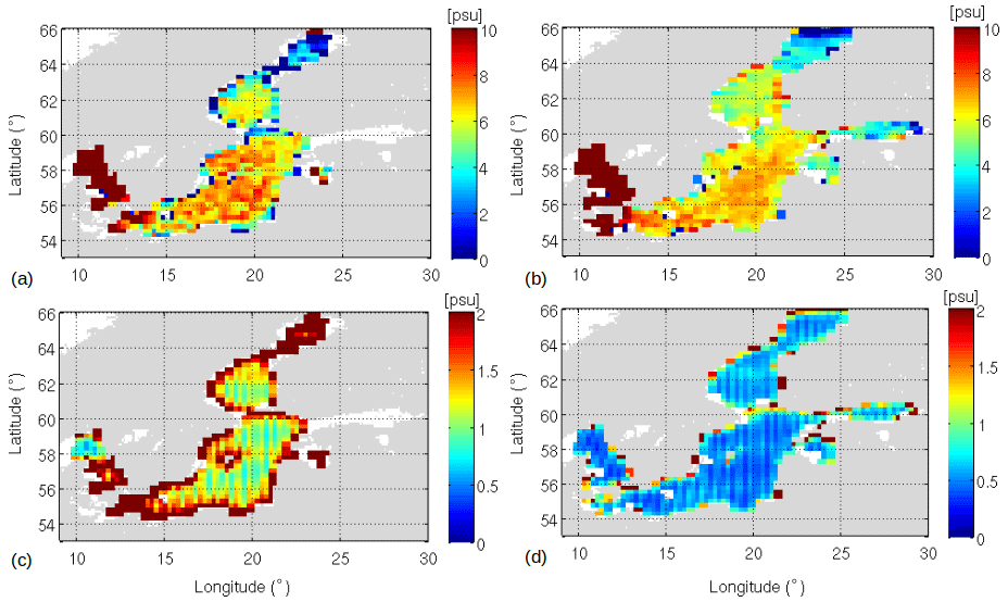
Figure 8(a) 9 d 0.25∘ L3 SSS map 15 to 23 January 2017, (b) 9 d 0.25∘ L3 SSS map 15 to 23 July 2017, (c) error of SSS map in (a), (d) error of SSS map in (b).
An example of a L3 SSS map and its associated error are shown in Fig. 8 for the cold (November to May) and warm (June to October) seasons. The estimated SSS error in the L3 product comes from the propagation of the errors in the debiased non-Bayesian SSS (in essence, coming from radiometric errors on TB; see Eq. 1 in Olmedo et al., 2021b). Note the increase in uncertainty in the winter period (Fig. 8c) with respect to the summer period (Fig. 8d). These larger errors in the cold season are expected due to the loss of TB sensitivity to SSS changes at cold waters.
2.2.7 Correction of time-dependent biases
SMOS measurements are affected not only by spatial biases, but also by biases that depend on time (Martín-Neira et al., 2016). In the debiased non-Bayesian retrieval, time-dependent biases are not corrected: the SMOS-based climatologies integrate a multi-year period, providing a reference that is constant in time (Sect. “Characterization and correction of SMOS SSS systematic errors”). Therefore, an additional correction for the time-dependent biases is required.
In the BEC global product (Olmedo et al., 2021b), the assumption used to mitigate these time-dependent biases is that the spatial average of SSS anomalies in the global ocean is zero at any instant. This hypothesis has been shown to hold well with in situ SSS (Argo) in the global ocean. But this assumption is not suitable regionally, and even less so in the Baltic Sea due to the net exchanges of salinity across region boundaries. In other BEC regional SSS products, such as those of the Mediterranean Sea (Olmedo et al., 2018b) and the Arctic Ocean (Olmedo et al., 2018a), time-dependent biases were corrected by using Argo measurements as reference. However, due to the scarce spatiotemporal coverage of Argo floats (restricted to Bothnian Sea, Gotland Deep and Bornholm Deep), this approach cannot be applied in the Baltic Sea. Instead, we assess the temporal correction by using two different reference datasets: in situ measurements from SeaDataNet (Sect. 3.1.3) and the CMEMS Baltic reanalysis (Sect. 2.1.2). As it can be observed in Fig. 9, both corrections are in agreement. However, due to the lack of in situ measurements and their spatiotemporal inhomogeneity, the temporal correction computed with in situ data is much noisier and does not always provide a value for the correction, which leads to data gaps. For these reasons, the CMEMS Baltic reanalysis is used for the temporal correction.
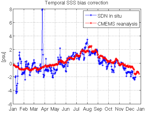
Figure 9Temporal bias correction computed for the SSS product during 2013 by using the CMEMS Baltic reanalysis (red) and SDN in situ measurements (blue). Note that the peaks in the correction computed from SDN in situ measurements are due to the very scarce and fragmentary spatial distribution of collocated in situ data.
2.2.8 Multifractal fusion of SSS and SST
L4 SSS product has been generated by applying multifractal fusion techniques (Umbert et al., 2014; Olmedo et al., 2016), which allows the noise of the SSS maps to be reduced (Turiel et al., 2014) without losing effective spatial resolution (Olmedo et al., 2016). The application of this technique is aimed at improving the spatiotemporal resolutions of the Baltic+ L3 SSS maps to approach user requirements (BEC team, 2021a).
The same SST data that are used as auxiliary data in the SSS retrieval are used here as template in the fusion scheme. L4 SSS maps are produced with the same spatiotemporal resolutions as the template, i.e., daily maps at a spatial grid of . Before applying the fusion, the salinity field from CMEMS Baltic reanalysis is used to complete the coverage where SMOS L3 SSS is not available. Salinities from reanalysis are previously filtered by using the SIF information available in the OSTIA SST product. Figure 10 shows the number of times per year (as a ratio to one) where the salinity reanalysis is used at each grid cell of the L4 map. Overall, those regions with extrapolated values coming from the reanalysis are reduced to the gulfs, Bothnian Bay and in those cell grids closest to the coast. As can be observed, during the first period of the mission (mainly during 2011–2012), the reanalysis is also occasionally used in other regions when the maps are strongly affected by RFI contamination (Oliva et al., 2016). For filtering purposes, a flag included in the product indicates if the SSS provided at each pixel comes from an extrapolated reanalysis value.
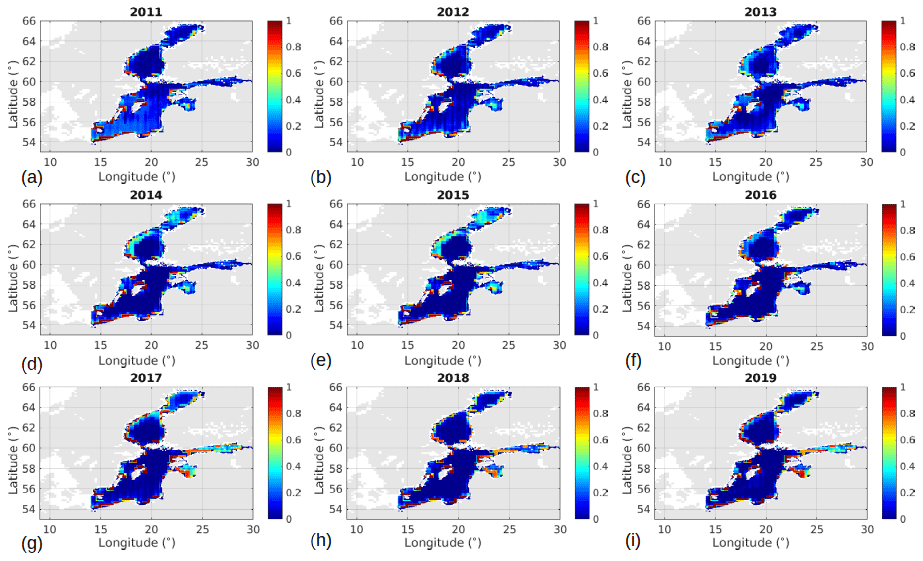
Figure 10Ratio of time when the SSS from CMEMS Baltic reanalysis is used in those grid points where the SMOS SSS L3 product is not available (from a 2011 to i 2019).
2.2.9 Estimation of the L4 SSS error
To assess the inherent uncertainty of the L4 SSS product, the correlated triple collocation (CTC) method is used (González-Gambau et al., 2020).
When applying CTC, the data are assumed to represent similar spatiotemporal scales with two of the datasets possibly having correlated errors. Under these conditions, CTC can be used to obtain maps of error variances of triplets of remote sensing SSS maps.
We consider three sets of collocated SSS maps in the period 2016–2018: (i) Baltic+ L4 SSS product, (ii) CMEMS Baltic reanalysis product (Axell, 2019) and (iii) the BSIOM hindcast simulation (Sect. 2.1.6). As shown in Fig. 8, the L3 SSS error during the cold season is higher than in the warmer season. Since the expected errors are quite different between both seasons, we performed the CTC analysis for the warm and the cold seasons separately. This analysis is done with all the products reduced to the common resolution (that of Baltic+ L4, 0.05∘ and daily frequency). Figure 11 shows the estimated error standard deviations of Baltic+ L4 SSS. L4 SSS errors are around 0.4–0.6 psu. These errors are in agreement with the differences found in the comparison to in situ measurements (see Sect. 3.4). There is a very significant error reduction in the L4 SSS with respect to the L3 SSS (0.6–0.9 psu; see Sect. 3.4.3). Note that, unlike the overall reduction of the error in the warmer season for the L3 SSS product, in the case of the L4 SSS product there is not a clear improvement for any of the seasons. This is likely due to the errors present in the SST employed as a template in the fusion scheme for the generation of the L4 SSS product.
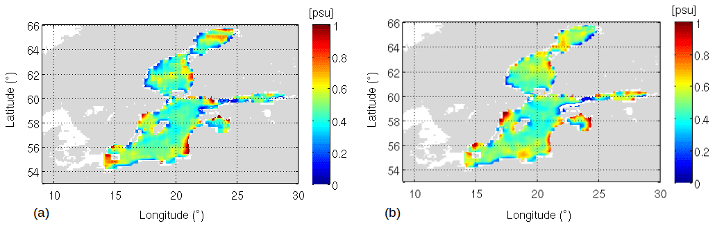
Figure 11Error standard deviations computed by CTC for Baltic+ L4 SSS during the (a) cold season and (b) warm season.
3.1 Datasets for validation
3.1.1 Satellite sea surface salinity
We compare the performance of the new Baltic+ SSS to those of other existing EO SSS products. The satellite SSS products used for this inter-comparison are the following:
-
SMOS CATDS: 9 d SMOS SSS maps provided by Centre Aval de Traitement des Données SMOS (CATDS). We use the L3 debiased v5 freely available at https://www.seanoe.org/data/00417/52804/#79565 (last access: 22 June 2021) (Boutin et al., 2018, 2020).
-
ESA CCI: 7 d CCI SSS product. We use the v1.7 (Boutin et al., 2019).
-
SMAP JPL: 8 d SMAP SSS maps are provided by Jet Propulsion Laboratory (JPL). We use the Level 3 version 4.2 freely available at https://podaac.jpl.nasa.gov/dataset/SMAP_JPL_L3_SSS_CAP_8DAY-RUNNINGMEAN_V42 (last access: 10 May 2022) (JPL Climate Oceans and Solid Earth group, 2019; Fore et al., 2016).
-
SMAP REMSS: 8 d running Remote Sensing Systems SMAP. We use the Level 3 Sea Surface Salinity Standard Mapped Image version v4, which is freely available at http://www.remss.com/missions/smap (last access: 22 June 2021). In particular, we have used the smoothed measurement at approximately 70 km resolution (Remote Sensing Systems, 2019; Meissner et al., 2018).
Figure 12 shows the spatiotemporal coverage during 2016 (percentage of valid SSS retrievals with respect to the total number of maps in the year) for each one of the above-mentioned satellite SSS products. The SMOS CATDS product shows very limited temporal and spatial coverage. SMAP JPL L3 SSS product exhibits a very good temporal and spatial coverage and SMAP REMSS covers mainly the central part of the basin with a good temporal coverage. The ESA CCI SSS product, developed from SMOS and SMAP measurements, shows a very limited spatial coverage but with good temporal coverage.
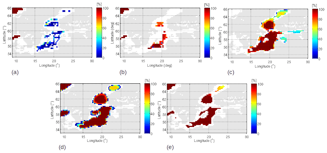
Figure 12Spatiotemporal coverage of year 2016 (percentage of valid SSS retrievals with respect to the total number of maps in the year) for each satellite product: (a) SMOS CATDS, (b) ESA CCI, (c) Baltic+ L3 SSS, (d) SMAP JPL, (e) SMAP REMSS.
3.1.2 FerryBox lines in situ salinity
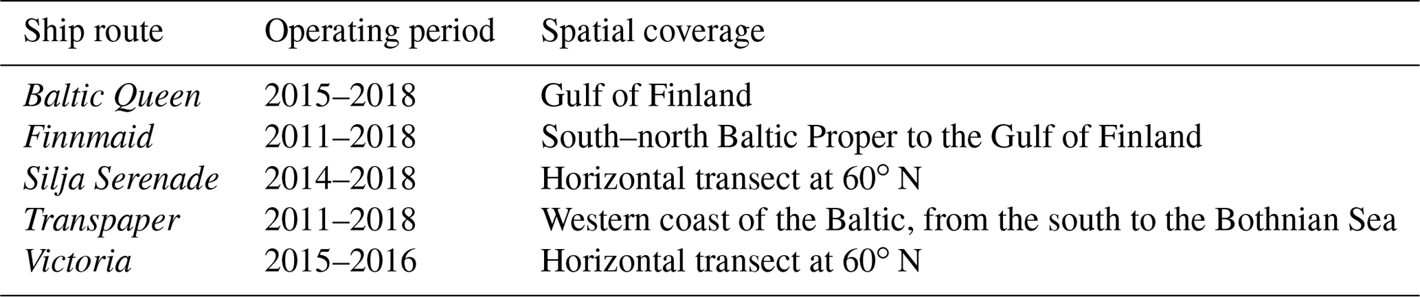
Ship tracks from the FerryBox voluntary network measure both temperature and salinity in mounted thermosalinographs (TSGs) on voluntary vessels routinely making transects in the Baltic Sea. These data were available at CMEMS under the product identifier INSITU_BAL_TS_REP_OBSERVATIONS_013_038 (it was retired in March 2020 and replaced by INSITU_GLO_TS_REP_OBSERVATIONS_013_001_b; https://doi.org/10.17882/46219, Tanguy et al., 2019).
The data collected from these vessels pass quality control checks before being distributed to the science community. All the ship routes available for the validation of Baltic+ SSS products are collected in Table 2. They are used for validation depending on data availability (i.e., each ship track has a different operating time), and its quality check passed as “good data”.
3.1.3 SeaDataNet and ICES in situ salinity
The SeaDataNet (SDN) Temperature and Salinity historical data collection for the Baltic Sea V2 (https://doi.org/10.13155/78589, Örjan et al., 2020) contains all open-access temperature and salinity in situ data retrieved from SeaDataNet infrastructure (CTD and discrete water samplers) until the end of 2014. Data have been quality-checked using Ocean Data View software. Quality flags of anomalous data have been revised using basic quality control procedures. For this validation, the following SSS and SST quality control provided within the SDN dataset is applied: var3_qc=49 (good quality of SSS) and var2_qc=49 (good quality of SST).
The in situ data in the period 2015–2019 were downloaded from ICES (International Council for the Exploration of the Sea) Oceanography CTD and bottle data (nowadays ICES Data Portal https://www.ices.dk/, last access: 14 May 2020). Data quality in ICES is solely the responsibility of the data originator, though the ICES data center may do random quality checks for the data.
Furthermore, to keep consistency with the other datasets, the uppermost available SSS measurements are used for this validation, lying in the range of 1–5 m depth.
3.2 Validation methods
Collocation strategy of satellite in situ data
The collocation strategy we follow for the comparison to in situ is the following:
-
Spatial collocation
-
FerryBox lines. These datasets provide SSS information at a very high temporal frequency. The location of in situ data are gridded to the nearest satellite grid cell, so all the in situ measurements corresponding to the same cell grid in the satellite SSS product (0.25∘ in the case of the L3 product and 0.05∘ in the L4 product) are averaged.
-
SeaDataNet. In this dataset the temporal sampling is quite sparse. Several measurements in depth are available at each station. We consider that the water in the upper 5 m is homogeneously mixed and it is representative of the surface water. Thus, we keep the shallowest measurement acquired between 1–5 m depth, to be compared with the satellite SSS. The location of in situ data are referred to the nearest satellite grid cell and compared to the corresponding Baltic+SSS measurement. In this case, in contrast to the case of the FerryBox measurements, almost no average of in situ data in a single grid is expected.
-
-
Temporal collocation
-
For all the datasets, all the in situ data available in the 9 days (for L3 product) of SMOS data used to generate the product and in the same day (for L4 product) of the map are considered in the comparison.
-
3.3 Quality metrics for the comparison to in situ
The quality assessment of the SSS satellite retrievals results from the comparison against the reference datasets presented in Sect. 3.1.2 and 3.1.3. The validation metrics are based on statistical measurements of the difference between the two quantities at the collocations ().
The following metrics are computed both for Baltic+ L3 and L4 SSS products:
-
Global statistics of ΔSSS for the datasets per year.
-
Analysis of the product performances in the cold and warm seasons separately. The separation in these two periods is based in the expected SST ranges for the different months and the expected SSS error due to those SST values. The cold season ranges from November to May (average temperature of 3.9 ∘C), and the warm season refers to the period of June to October (average temperature of 13.4 ∘C). This analysis per season is devoted to assessing if a quality improvement is observed during the warmer months, since the sensitivity increases and lower SSS errors than at colder temperatures are expected.
-
Maps of the spatial distributions of ΔSSS statistics. The temporal mean and the temporal standard deviation of ΔSSS are computed for each grid point in the map. This metric is devoted to track the possible origin of the errors (residual land sea contamination, sea-ice contamination, ice contamination itself, etc).
3.3.1 Correlated triple collocation
The three satellite SSS products with the best temporal and spatial coverage (see Sect. 3.1.1) are inter-compared. It must be pointed out that the salinity values provided by each one of the three satellite products are very different between them. We applied the CTC analysis using a 1-year period (2016), which suffices to evaluate the performance of the datasets. Three sets of collocated SSS maps are considered: JPL SMAP v4.2 SSS, 8 d maps; REMSS SMAP v4.0 SSS, 8 d maps; and Baltic+ L3 SSS, 9 d maps. We only consider Baltic+ L3 SSS here because it is the product with similar spatiotemporal resolutions to JPL and REMSS SMAPS maps, a condition needed to apply the CTC method. In this triplet, the two variables with correlated errors are the JPL and REMSS products, both from SMAP measurements. Time collocation is done by identifying the first day of the three periods used in the generation of the corresponding maps. As JPL SMAP and REMSS SMAP maps are 1 d shorter, time collocation is not perfect but differences are considered to be negligible taking into account the orbital gaps in a 9 d period. Spatial collocation is straightforward, since the three products are provided in the same grid.
3.3.2 Baltic+ SSS variability and comparison to reanalysis and in situ data
The objective of this assessment is to analyze the SSS dynamics captured by Baltic+ SSS products and the CMEMS Baltic reanalysis (Axell, 2019) and to compare them to the 22 in situ observation stations visited by research vessels (Fig. 13). Those stations are intended to cover different types of sea areas: from coastal regions to open sea. We choose the uppermost salinity observations, which means observations from 1–1.5 m depth.
Time series of Baltic+ L3 and L4 SSS products are analyzed and compared to the salinity provided by the CMEMS Baltic reanalysis and the in situ measurements. For that, we define boxes over given regions of interest, where both the reanalysis salinity and the Baltic+ L3 and L4 SSS products are averaged and compared to the in situ stations that are located in the region defined by each box. The boxes used for each region are shown in Fig. 13.
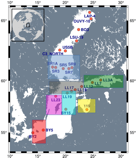
Figure 13Map of the in situ stations and the boxes used in the analysis of the time series per region. Red: Arkona Basin, grey: northern Baltic Proper, blue: Bothnian Sea, cyan: eastern Gotland Basin, pink: western Gotland Basin, green: Gulf of Finland, yellow: Gulf of Riga.
3.4 Validation results
3.4.1 Comparison to FerryBox lines salinity
All the in situ measurements from the different ferry routes are analyzed per year. The statistics are computed considering all the collocations available for the Baltic+ L3 SSS product and FerryBox data (see Table 3, first row). Note that the number of match-ups corresponds to all the collocated measurements of SMOS and ferry data. Overall, similar statistics are obtained for all the years. In the year 2012 there is a significant reduction of the accuracy due to the strong RFI affectation in the North Atlantic for that period (Oliva et al., 2016). Slightly higher biases are found for the years 2014 and 2015.
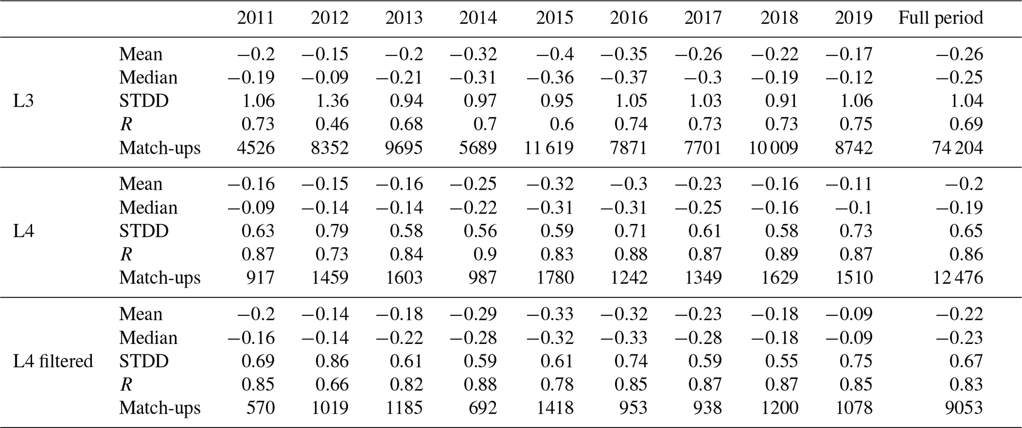
Table 3Global statistics for Baltic+ L3, L4 and filtered L4 (not considering extrapolated measurements from reanalysis) SSS products against FerryBox in situ data. Note the high variability in the number of match-ups is due to the different cruises operated each year.

To analyze the spatial distribution of the differences (ΔSSS) between the Baltic+ L3 SSS product and the in situ data provided by ferry lines, we compute the mean of ΔSSS (Fig. 14), and the standard deviation of ΔSSS (Fig. 15), for all the measurements accumulated during 1 year, for each cell of the Baltic+ L3 SSS product grid. The number of match-ups is shown in Fig. 16. Note that only grid cells with more than 10 accumulated measurements are considered. Higher standard deviation values are obtained for those cells closer to coast and ice edges, particularly close to Gotland, in the Arkona and Bornholm basins, and in the Bothnian Bay. Errors in these regions notably increase the standard deviation when computing the statistics considering all the match-up differences (see Table 3, first row).
To analyze the spatial distribution without the effect of the non-homogeneous spatial sampling, the histograms of the spatial distributions of the mean and the standard deviation of ΔSSS are computed (not shown). The most probable value of the mean ΔSSS for the L3 product is in the range of [−0.35 to −0.15], and the most probable value for the standard deviation of ΔSSS ranges between [0.57 to 0.72], depending on the year and it reaches 0.97 for the year 2012 (affected by strong RFI contamination).
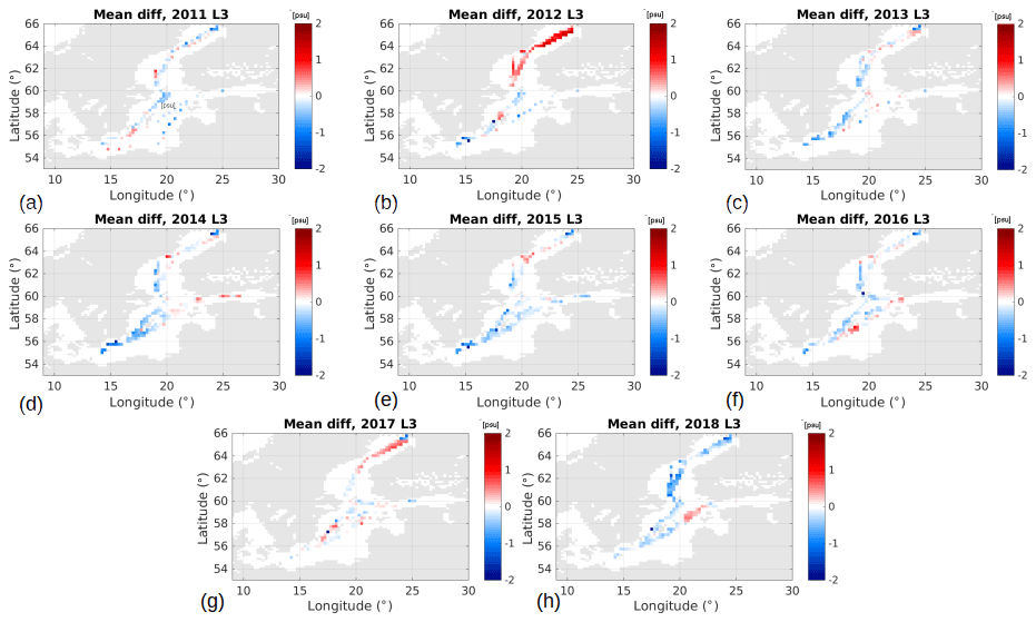
Figure 14Comparison of L3 SSS and ferry data: spatial distribution of the mean of ΔSSS [psu] per year (from a 2011 to h 2018). The reason behind the positive biases for years 2012 and 2017 in the Gulf of Bothnian is under investigation.
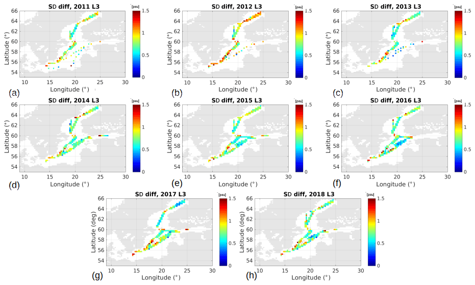
Figure 15Comparison of L3 SSS and ferry data: spatial distribution of the standard deviation of ΔSSS [psu] per year (from a 2011 to h 2018).

Figure 16Comparison of L3 SSS and ferry data: number of match-ups for each grid point in the map per year (from a 2011 to h 2018).
Global statistics are also computed considering all the collocations available for the Baltic+ L4 SSS product and FerryBox data (see Table 3, middle row). We can observe a clear reduction of the standard deviation and an increase in the correlation coefficient with respect to the statistics computed for the L3 SSS product (see Table 3, first row). Similar biases to the ones for L3 product are found for the L4 product. This is expected because the fusion methodology aims to reduce the standard deviation of the error but not the biases present in the original L3 maps (Turiel et al., 2014).
We also compute global statistics of the collocations of Baltic+ L4 SSS and FerryBox data per year, considering only those Baltic+ L4 SSS that come from the L3 SSS (i.e., extrapolated data from reanalysis are filtered out) (see Table 3, last row). As can be seen by comparing to the statistics considering all the measurements in the L4 product (Table 3, middle row), statistics have not significantly changed.
The spatial differences between the L4 SSS and the SSS provided by ferry data are computed in 0.05∘ grid of the L4 product (not shown). However, due to the low number of accumulated measurements for each grid cell, measurements are accumulated in a coarser grid (0.25∘) to have significant statistics (see Figs. 17, 18, 19). Besides, grid cells with accumulated measurements lower than 10 are filtered out. The standard deviation is reduced in all the basin with respect to the L3 product (see Fig. 18 in comparison to Fig. 15). The histograms of the spatial distributions of the mean and the standard deviation of ΔSSS are also computed. The most probable value of the mean ΔSSS for the L4 product is in the range of [−0.35 to −0.25] psu and the most probable value for the standard deviation of ΔSSS ranges between [0.33. to 0.47] psu, depending on the year.
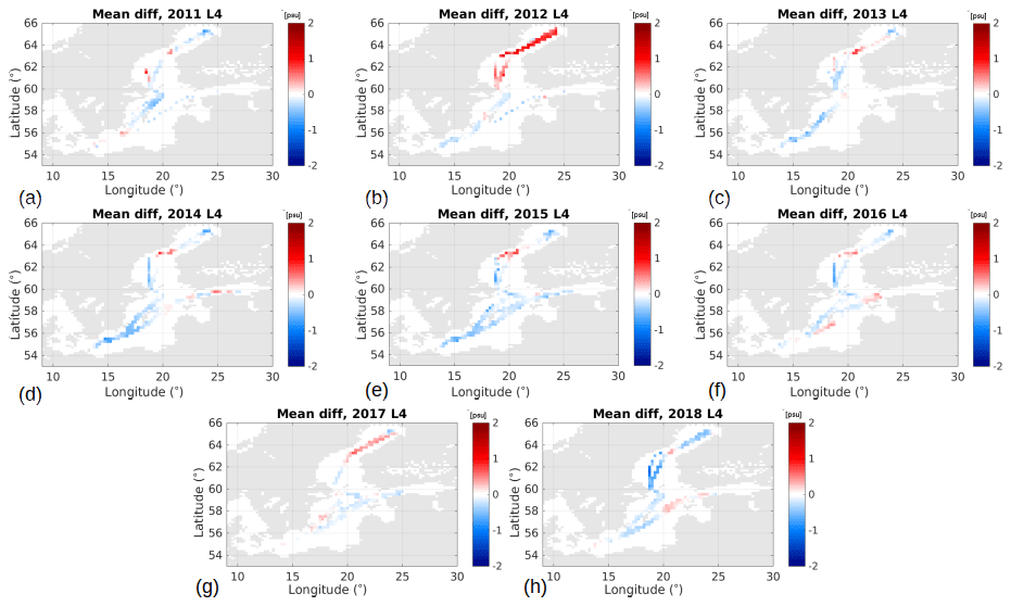
Figure 17Comparison of L4 SSS and ferry data: spatial distribution of mean ΔSSS [psu] per year (from a 2011 to h 2018).
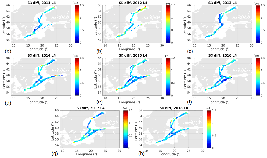
Figure 18Comparison of L4 SSS and ferry data: spatial distribution of the standard deviation of ΔSSS [psu] per year (from a 2011 to h 2018).
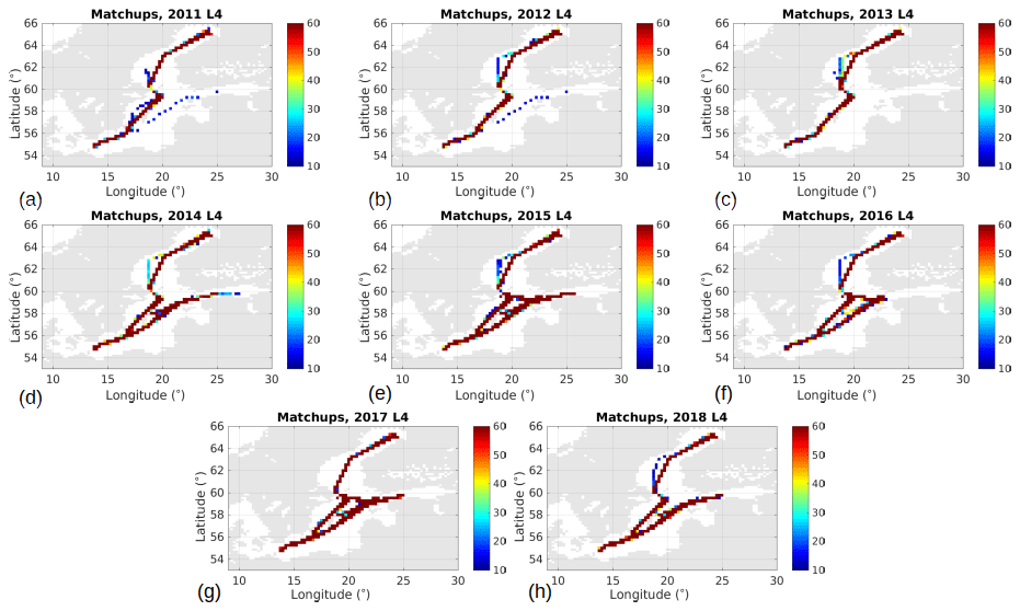
Figure 19Comparison of L4 SSS and ferry data: number of match-ups for each grid point in the map per year (from a 2011 to h 2018).
3.4.2 Comparison to SeaDataNet salinity
Global statistics are computed considering all the collocations available for the Baltic+ L3 SSS product and SeaDataNet data per year (see Table 4, first row). Overall, statistics are in agreement with the statistics of the comparison to the FerryBox data. However, higher values of standard deviation are obtained. This is likely due to the fact that Arkona and Bornholm basins are highly sampled with respect to the rest of the Baltic Sea and these regions present higher SSS errors.
Table 4Global statistics of Baltic+ L3, L4 and filtered L4 (not considering extrapolated measurements from reanalysis) SSS products against SeaDataNet in situ data.
The spatial distribution of the SeaDataNet in situ measurements allows us to analyze the performances of the Baltic+ L3 SSS product in the whole Baltic Basin and the influence of the proximity to land and ice edges in the quality of the Baltic+ SSS products. We compute the mean of ΔSSS and the standard deviation of ΔSSS for all the measurements accumulated for each cell of the Baltic+ L3 SSS product grid. Measurements are accumulated in the original L3 grid (0.25∘) for all 9 years, since there are not enough in situ observations to perform the analysis per year separately, as we do in the case of FerryBox data. Since the number of match-ups is still quite limited, we compute the same maps by accumulating the measurements in a 0.5∘ grid. In this way, we increase the number of measurements in each cell to get significant statistics. In addition, all those grid cells with less than 10 measurements are discarded. Higher errors are detected in Arkona and Bornholm basins, which are highly sampled regions. We also repeat this spatial analysis for the cold and the warm seasons. In the warm season the standard deviation is significantly reduced with respect to the cold season, as expected. The most probable value of the mean ΔSSS for the L3 product is −0.15 in the cold season and −0.35 during the warm season. For the standard deviation of ΔSSS, the most probable value is around 0.72 in the warm season and 0.78 in the cold season, although another mode appears around 1.05.
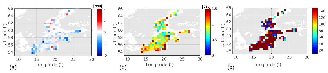
Figure 20Comparison of L3 SSS and SDN: Spatial distribution of ΔSSS [psu] with SDN in a coarser grid (0.5∘): (a) mean, (b) standard deviation, (c) number of match-ups.
Global statistics are computed considering all the collocations available for the Baltic+ L4 SSS product and SeaDataNet data per year (see Table 4, middle row). Overall, statistics are in agreement with the statistics of the comparison to the ferry data. However, higher values of standard deviation have been obtained. This is likely due to the fact that Arkona and Bornholm basins are highly sampled with respect to the rest of the Baltic Sea basin and these regions present higher SSS errors. In any case, the improvement in terms of the standard deviation and correlation coefficient with respect to the L3 SSS product is very significant (see Table 4, first row).
Global statistics are also computed considering all the collocations available for the Baltic+ L4 SSS product when the extrapolation of the reanalysis data is not considered and SeaDataNet data per year (see Table 4, last row). As can be observed by comparing to the statistics when considering all the measurements in the L4 product, statistics have not significantly changed for most of the years. Higher differences are found for the years 2011 and 2012, where the extrapolated data are not limited to the coastal pixels (see Fig. 10).
The spatial distribution of the differences between the Baltic+ L4 SSS product (considering all the measurements) and the in situ data provided by SeaDataNet is also analyzed. For that, we compute the mean of ΔSSS and the standard deviation of ΔSSS for all the measurements accumulated in each cell of a 0.5∘ grid (to get significant statistics) (see Fig. 21). Measurements have been accumulated for all 9 years since the match-ups are not enough to perform the analysis per year separately. In agreement with the analysis of the L3 product, higher errors are detected in Arkona and Bornholm basins, which are highly sampled regions. We perform this spatial analysis for the cold and the warm seasons separately. Once again, for the warm season the standard deviation is reduced with respect to the cold season, as expected. The most probable value of the mean ΔSSS for the L4 product is −0.25 in the cold season and −0.35 during the warm season. For the standard deviation of ΔSSS, the most probable value is around 0.47 in the warm season, while during the cold season it is around 0.53.
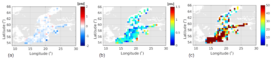
Figure 21Comparison of L4 SSS and SDN, spatial distribution of ΔSSS [psu] (0.5∘ grid): (a) mean, (b) standard deviation, (c) number of match-ups.
3.4.3 Estimated SSS uncertainty by CTC
Maps of the estimated error standard deviations for each SSS dataset are shown in Fig. 22. Notice that the estimated errors for the Baltic+ L3 SSS are in agreement with the differences found with respect to in situ measurements (see Sect. 3.4.1 and 3.4.2). Differences between both SMAP products and the Baltic+ L3 SSS are shown in Fig. 23. As shown in the figure, the Baltic+ L3 SSS product has the smallest error in the whole basin, except in some grid points of the Bothnian Bay, where the SMAP REMSS product presents a lower error.
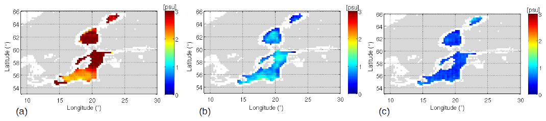
Figure 22Error standard deviations [psu] for the satellite SSS products computed by CTC for all the collocated maps in 2016: (a) SMAP-JPL (mean error in the basin: 2.81 psu), (b) SMAP-REMSS (mean error: 0.83 psu), (c) Baltic+ L3 SSS (mean error: 0.56 psu).
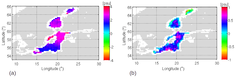
Figure 23(a) Difference between SMAP JPL and Baltic+ L3 SSS error standard deviations [psu], (b) difference between SMAP REMSS and Baltic+ L3 SSS error standard deviations.
The analysis of the Baltic+ L3 SSS product and the comparison with the other satellite products reveals that the Baltic+ L3 SSS product is currently the satellite-derived SSS product with the lowest salinity error among the currently available products, highlighting especially the improved spatial coverage and oceanographic resolution.
3.4.4 Description of salinity dynamics
Figure 24 shows the spatiotemporal collocations of the Baltic+ L3 and L4 SSS products and reanalysis with in situ measurements. It must be pointed out that the sampling frequency is too low to capture some relevant events in some in situ stations, as for example in the regions of the Bothnian Sea and the Gulf of Riga. An overall agreement in the main events is observed between satellite, model and in situ data along the time series. However, salinity from reanalysis shows a very stable behavior along the time series for some particular regions, while the variability shown by the satellite SSS better reflects the variability captured by the in situ measurements. This is observed very clearly in the northern Baltic Proper, in the eastern and western Gotland Basin and in the Gulf of Riga.
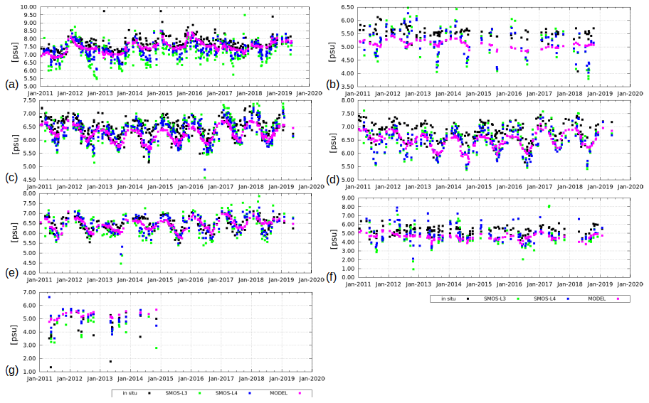
Figure 24Spatiotemporal collocations of Baltic+ L3 SSS, Baltic+ L4 SSS, CMEMS Baltic reanalysis salinity fields with in situ salinity. Regions: (a) Bornholm Basin (BB), (b) Bothnian Sea (BS), (c) northern Baltic Proper (NBP), (d) eastern Gotland Basin (EGB), (e) western Gotland Basin (WGB), (f) Gulf of Finland (GOF) and (g) Gulf of Riga (GOR).
Baltic+ SSS products can be very useful to validate the models in areas where in situ data are sparse. Also, the location of the salinity gradients and their variability is valuable knowledge in evaluating the model performance. For example, Westerlund et al. (2018) discussed that model development is needed to better capture the large salinity gradients in the Gulf of Finland, but this work is hindered by the low temporal coverage of the data and lack of measurements from the eastern part of the Gulf of Finland. The same is also true for other sub-basins of the Baltic Sea and, especially, for the northern parts (Bothnian Sea and Bothnian Bay), where monitoring data are still too sparse. Thus, the new products will foster model development and provide the possibility to assimilate SSS fields derived from space assets.
Access to the data is provided by the Barcelona Expert Center, through its FTP service. The DOI of the L3 product is https://doi.org/10.20350/digitalCSIC/13859 (González-Gambau et al., 2021a). The DOI of the L4 product is https://doi.org/10.20350/digitalCSIC/13860 (González-Gambau et al., 2021b). Seasonal averaged L4 SSS products are also available in the HELCOM catalogue (https://metadata.helcom.fi/geonetwork/srv/eng/catalog.search#/metadata/9d979033-1136-4dd1-a09b-7ee9e512ad14, BEC team, 2021b), and they can be visualized in the HELCOM Map and Data service (https://maps.helcom.fi/website/mapservice/?datasetID=9d979033-1136-4dd1-a09b-7ee9e512ad14, last access: 9 November 2021).
In this work, we present the first regional satellite-derived SSS maps over the Baltic Sea. To date, these are unique dedicated remote sensed SSS products available over the region, mainly due to the technical difficulties of retrieving SSS from satellite measurements over this basin. Several technical improvements have been required, the major ones being (i) the study of the dielectric constant models for the low-salinity regimes of the Baltic Sea, and (ii) the characterization of SMOS SSS systematic errors depending also on the SST. These improvements developed in the context of the Baltic+ Salinity Dynamics project have a clear impact on other regional initiatives (such as EO4SIBS (4000127237/19/I-EF) and SO-Fresh (4000134536) projects) and in the SSS retrieval from satellite L-band measurements in general.
Baltic+ SSS products have been proven to have a good spatiotemporal coverage with an accuracy of 0.7–0.8 psu for the L3 product (9 d, 0.25∘) and around 0.4 psu in the case of the L4 product (daily, 0.05∘). Regions with higher errors and limited coverage are located in Arkona and Bornholm basins and the gulfs of Finland and Riga (Sect. 3). The impact assessment of Baltic+ SSS products reveals that they provide valuable information about the changes in the salinity gradients and about the temporal variability in the sea surface salinity. They also show a geophysically consistent seasonal variability in surface salinity, which results from the melting of sea ice in spring and increased run-off from land when snow cover melts after the winter. For all the above, Baltic+ SSS products can help in understanding the salinity dynamics of the basin. On the one hand, this EO SSS data can fill the temporal and spatial observational gaps in the region left by the very sparse in situ measurements. On the other hand, Baltic+ SSS products can also be useful for the validation and improvement of numerical models. As well as this, the capability of the Baltic+ SSS product to map the horizontal gradients and their variability is of much value to evaluate the performance of models and provide the possibility to assimilate SSS fields.
Several scientific studies with Baltic+ SSS data are currently in progress, such as (i) the analysis of the consistency between the structures detected in the Baltic+ SSS products with the ones detected in the SST and in the DOT (Dynamic Ocean Topography) and (ii) the use of Baltic+ SSS time series as part of the HELCOM indicators to study the correlation between the SSS variability and the extreme events of different species in the Baltic Sea. Interactions with the scientific communities working in the Baltic, and in particular with Baltic Earth Working Group on Salinity Dynamics, has allowed us to identify that Baltic+ SSS products can help fill some knowledge gaps (Lehmann et al., 2022), such as (i) the determination of the SSS annual trends in the basin in the last decade and (ii) the study of the inflow and outflow dynamics at the entrance of the North Sea. For these potential applications, some additional technical developments in the product would be appropriated, mainly focused on applying a temporal correction of SSS maps without using external references, and applying fusion techniques at brightness temperature level for improving their quality in terms of coverage and spatial scales.
VGG generated the BEC product and is the main contributor to the writing of this paper. EO and CGH were the main contributors to the editing of this paper. VGG, EO, AT and JM were responsible for the conceptualization and development of the algorithms used in the generation of the product. CGH was responsible for the distribution of the products. The validation of the products was carried out by CGH, AGE, NH, MU, CG and VGG. PA and LT provided quality-controlled in situ data and participated in the discussions about the quality of the product and potential applications. MA and RC were responsible for the management of the project. DF and RS were the ESA project officers. All authors have reviewed the paper.
The contact author has declared that neither they nor their co-authors have any competing interests.
Publisher’s note: Copernicus Publications remains neutral with regard to jurisdictional claims in published maps and institutional affiliations.
The authors would like to thank Andreas Lehman (Chair of the Baltic Earth Working Group on Salinity Dynamics, from GEOMAR Helmholtz-Zentrum für Ozeanforschung) for his valuable help on the definition of the scientific requirements and the scientific impact assessment of the products and to Klaus Getzlaff (also from GEOMAR Helmholtz-Zentrum für Ozeanforschung) for kindly providing the BSIOM hindcast simulation data.
They also would like to thank Jannica Haldin, Joni Kaitaranta, Kemal Pinarbasi and Owen Rowe (from The Baltic Marine Environment Protection Commission- HELCOM) for the fruitful discussions about the potential scientific applications of the Baltic+ SSS products and for integrating the seasonally averaged Baltic+ L4 SSS maps in HELCOM web map service. Last but not least, the authors want to acknowledge the anonymous reviewers and the editor for their valuable and helpful comments.
This work has been carried out as part of the Baltic+ Salinity Dynamics project (4000126102/18/I-BG), funded by the European Space Agency. It has been also supported in part by the Spanish R&D project INTERACT (PID2020-114623RB-C31), which is funded by MCIN/AEI/10.13039/501100011033. We also received funding from the Spanish government through the “Severo Ochoa Centre of Excellence” accreditation (CEX2019-000928-S). This work is a contribution to the CSIC Thematic Interdisciplinary Platform Teledetect.
This paper was edited by Giuseppe M. R. Manzella and reviewed by two anonymous referees.
Axell, L.: Product User Manual of Baltic Sea Physical Reanalysis Product BALTICSEA_REANALYSIS_PHY_003_011, issue 2.0, Tech. Rep., Copernicus Marine Environment Monitoring Service, https://catalogue.marine.copernicus.eu/documents/PUM/CMEMS-BAL-PUM-003-011.pdf (last access: 30 October 2019), 2019. a, b, c, d
BEC team: BEC Products Description, BEC-PD-SSS-Baltic-L3-L4.pdf, version1.0, July 2021, http://bec.icm.csic.es/doc/BEC_PD_SSS_Baltic_L3_L4.pdf (last access: 10 April 2022), 2021a. a
BEC team: Baltic+ L4 seasonal SSS product, Helcom catalogue [data set] https://metadata.helcom.fi/geonetwork/srv/eng/catalog.search#/metadata/9d979033-1136-4dd1-a09b-7ee9e512ad14 (last access: 10 April 2022), 2021b. a
Boutin, J., Vergely, J. L., Marchand, S., D'Amico, F., Hasson, A., Kolodziejczyk, N., Reul, N., Reverdin, G., and Vialard, J.: New SMOS Sea Surface Salinity with reduced systematic errors and improved variability, Remote Sens. Environ., 214, 115–134, https://doi.org/10.1016/j.rse.2018.05.022, 2018. a
Boutin, J., Vergely, J.-L., and Koehler, J.and Rouffi, F. R. N.: ESA Sea Surface Salinity Climate Change Initiative (Sea_Surface_Salinity_CCI): Version 1.8 data collection, CEDA Archive [data set], https://doi.org/10.5285/9ef0ebf847564c2eabe62cac4899ec41, 2019. a
Boutin, J., Vergely, J. L., and Khvorostyanov, D.: SMOS SSS L3 maps generated by CATDS CEC LOCEAN, debias V5.0, SEANOE [data set], https://doi.org/10.17882/52804#79565, 2020. a
Brown, M. A., Torres, F., Corbella, I., and Colliander, A.: SMOS Calibration, IEEE T. Geosci. Remote, 46, 646–658, https://doi.org/10.1109/TGRS.2007.914810, 2008. a
Canada Meteorological Center: CMC 0.2 deg global sea surface temperature analysis. Ver. 2.0., PO.DAAC, CA, USA [data set], https://doi.org/10.5067/GHCMC-4FM02, 2012. a
Corbella, I., Torres, F., Camps, A., Colliander, A., Martin-Neira, M., Ribo, S., Rautiainen, K., Duffo, N., and Vall-llossera, M.: MIRAS end-to-end calibration: application to SMOS L1 processor, IEEE T. Geosci. Remote, 43, 1126–1134, https://doi.org/10.1109/TGRS.2004.840458, 2005. a
Corbella, I., Torres, F., Duffo, N., Gonzalez, V., Camps, A., and Vall-llossera, M.: Fast Processing Tool for SMOS Data, in: IGARSS 2008 – 2008 IEEE International Geoscience and Remote Sensing Symposium, vol. 2, II-1152–II-1155, https://doi.org/10.1109/IGARSS.2008.4779204, 2008. a
Corbella, I., Torres, F., Camps, A., Duffo, N., and Vall-llossera, M.: Brightness-Temperature Retrieval Methods in Synthetic Aperture Radiometers, IEEE T. Geosci. Remote, 47, 285–294, https://doi.org/10.1109/TGRS.2008.2002911, 2009. a
Corbella, I., Durán, I., Wu, L., Torres, F., Duffo, N., Khazâal, A., and Martín-Neira, M.: Impact of Correlator Efficiency Errors on SMOS Land–Sea Contamination, IEEE Geosci. Remote S., 12, 1813–1817, https://doi.org/10.1109/LGRS.2015.2428653, 2015. a, b, c
Corbella, I., González-Gambau, V., Torres, F., Duffo, N., Durán, I., and Martín-Neira, M.: The MIRAS “ALL-LICEF” calibration mode, in: 2016 IEEE International Geoscience and Remote Sensing Symposium (IGARSS), 2013–2016, https://doi.org/10.1109/IGARSS.2016.7729519, 2016. a
Corbella, I., Torres, F., Duffo, N., Durán, I., González-Gambau, V., and Martín-Neira, M.: Wide Field of View Microwave Interferometric Radiometer Imaging, Remote Sensing, 11, 682, https://doi.org/10.3390/rs11060682, 2019. a
Donlon, C. J., Martin, M., Stark, J., Roberts-Jones, J., Fiedler, E., and Wimmer, W.: The Operational Sea Surface Temperature and Sea Ice Analysis (OSTIA) system, Remote Sens. Environ., 116, 140–158, https://doi.org/10.1016/j.rse.2010.10.017, 2012. a, b, c
Fischer, H. and Matthäus, W.: The importance of the Drogden Sill in the Sound for Major Baltic Inflows, J. Marine Syst., 9, 137–157, https://doi.org/10.1016/S0924-7963(96)00046-2, 1996. a
Fore, A., Yueh, S., Tang, W., Stiles, B., and Hayashi, A.: Combined Active/Passive Retrievals of Ocean Vector Wind and Sea Surface Salinity With SMAP, IEEE T. Geosci. Remote, 54, 7396–7404, https://doi.org/10.1109/TGRS.2016.2601486, 2016. a
González-Gambau, V., Turiel, A., Olmedo, E., Martínez, J., Corbella, I., and Camps, A.: Nodal Sampling: A New Image Reconstruction Algorithm for SMOS, IEEE T. Geosci. Remote, 54, 2314–2328, https://doi.org/10.1109/TGRS.2015.2499324, 2015. a
González-Gambau, V., Olmedo, E., Turiel, A., Martínez, J., Ballabrera-Poy, J., Portabella, M., and Piles, M.: Enhancing SMOS brightness temperatures over the ocean using the nodal sampling image reconstruction technique, Remote Sens. Environ., 180, 205–220, https://doi.org/10.1016/j.rse.2015.12.032, 2016. a
González-Gambau, V., Olmedo, E., Martínez, J., Turiel, A., and Durán, I.: Improvements on Calibration and Image Reconstruction of SMOS for Salinity Retrievals in Coastal Regions, IEEE J. Sel. Top. Appl., 10, 3064–3078, https://doi.org/10.1109/JSTARS.2017.2685690, 2017. a, b, c
González-Gambau, V., Turiel, A., González-Haro, C., Martínez, J., Olmedo, E., Oliva, R., and Martín-Neira, M.: Triple Collocation Analysis for Two Error-Correlated Datasets: Application to L-Band Brightness Temperatures over Land, Remote Sensing, 12, 2281, https://doi.org/10.3390/rs12203381, 2020. a
González-Gambau, V., Olmedo, E., González-Haro, C., García-Espriu, A., and Turiel, A.: Baltic Sea Surface Salinity L3 maps, DIGITAL.CSIC [data set], https://doi.org/10.20350/digitalCSIC/13859, 2021a. a, b
González-Gambau, V., Olmedo, E., González-Haro, C., García-Espriu, A., and Turiel, A.: Baltic Sea Surface Salinity L4 maps, DIGITAL.CSIC [data set], https://doi.org/10.20350/digitalCSIC/13860, 2021b. a, b
Hordoir, R., Axell, L., Höglund, A., Dieterich, C., Fransner, F., Gröger, M., Liu, Y., Pemberton, P., Schimanke, S., Andersson, H., Ljungemyr, P., Nygren, P., Falahat, S., Nord, A., Jönsson, A., Lake, I., Döös, K., Hieronymus, M., Dietze, H., Löptien, U., Kuznetsov, I., Westerlund, A., Tuomi, L., and Haapala, J.: Nemo-Nordic 1.0: a NEMO-based ocean model for the Baltic and North seas – research and operational applications, Geosci. Model Dev., 12, 363–386, https://doi.org/10.5194/gmd-12-363-2019, 2019. a
IOC, SCOR, and IAPSO: The international thermodynamic equation of seawater – 2010: Calculation and use of thermodynamic properties, Intergovernmental Oceanographic Commission, Manuals and Guides No. 56, UNESCO (English), 196 pp., https://www.teos-10.org/pubs/TEOS.10_Manual.pdf (last access: 1 April 2022), 2010. a
JPL Climate Oceans and Solid Earth group: JPL SMAP Level 3 CAP Sea Surface Salinity Standard Mapped Image 8-Day Running Mean V4.2 Validated Dataset. Ver. 4.2., Physical Oceanography Distributed Active Archive Center, CA, USA [data set], https://doi.org/10.5067/SMP42-3TPCS, 2019. a
Klein, L. and Swift, C.: An improved model for the dielectric constant of sea water at microwave frequencies, IEEE J. Oceanic Eng., 2, 104–111, https://doi.org/10.1109/JOE.1977.1145319, 1977. a
Lehmann, A., Hinrichsen, H.-H., Getzlaff, K., and Myrberg, K.: Quantifying the heterogeneity of hypoxic and anoxic areas in the Baltic Sea by a simplified coupled hydrodynamic-oxygen consumption model approach, J. Marine Syst., 134, 20–28, https://doi.org/10.1016/j.jmarsys.2014.02.012, 2014. a
Lehmann, A., Myrberg, K., Post, P., Chubarenko, I., Dailidiene, I., Hinrichsen, H.-H., Hüssy, K., Liblik, T., Meier, H. E. M., Lips, U., and Bukanova, T.: Salinity dynamics of the Baltic Sea, Earth Syst. Dynam., 13, 373–392, https://doi.org/10.5194/esd-13-373-2022, 2022. a, b, c
Leppäranta, M. and Myrberg, K.: The Physical Oceanography of the Baltic Sea, edited by: Blondel, P., University of Bath, UK, Springer‐Verlag, Berlin‐Heidelberg, New York, ISBN: 978-3-540-79702-9, 2009. a, b
Martín-Neira, M., Oliva, R., Corbella, I., Torres, F., Duffo, N., Durán, I., Kainulainen, J., Closa, J., Zurita, A., Cabot, F., Khazaal, A., Anterrieu, E., Barbosa, J., Lopes, G., Tenerelli, J., Díez-García, R., Fauste, J., Martín-Porqueras, F., González-Gambau, V., Turiel, A., Delwart, S., Crapolicchio, R., and Suess, M.: SMOS instrument performance and calibration after six years in orbit, Remote Sens. Environ., 180, 19–39, https://doi.org/10.1016/j.rse.2016.02.036, 2016. a, b
Matthäus, W. and Franck, H.: Characteristics of major Baltic inflows – a statistical analysis, Cont. Shelf Res., 12, 1375–1400, https://doi.org/10.1016/0278-4343(92)90060-W, 1992. a
Meier, H. E. M., Kjellström, E., and Graham, L. P.: Estimating uncertainties of projected Baltic Sea salinity in the late 21st century, Geophys. Res. Lett., 33, L15705, https://doi.org/10.1029/2006GL026488, 2006. a
Meissner, T. and Wentz, F. J.: The complex dielectric constant of pure and sea water from microwave satellite observations, IEEE T. Geosci. Remote, 42, 1836–1849, https://doi.org/10.1109/TGRS.2004.831888, 2004. a, b
Meissner, T., Wentz, F. J., and Manaster, A.: Remote Sensing Systems SMAP Ocean Surface Salinities [Level 2C, Level 3 Running 8-day, Level 3 Monthly], Version 3.0 validated release, Tech. Rep., Remote Sensing Systems, Santa Rosa, CA, USA, https://doi.org/10.5067/SSSSS-TTTTT, 2018. a, b
Merchant, C. J., Embury, O., Bulgin, C. E., Block, T., Corlett, G. K., Fiedler, E., Good, S. A., Mittaz, J., Rayner, N. A., Berry, D., Eastwood, S., Taylor, M., Tsushima, Y., Waterfall, A., Wilson, R., and Donlon, C.: Satellite-based time-series of sea-surface temperature since 1981 for climate applications, Scientific Data, 6, 223, https://doi.org/10.1038/s41597-019-0236-x, 2019. a, b
Mohrholz, V.: Major Baltic Inflow Statistics – Revised, Frontiers in Marine Science, 5, https://doi.org/10.3389/fmars.2018.00384, 2018. a
Oliva, R., Daganzo, E., Richaume, P., Kerr, Y., Cabot, F., Soldo, Y., Anterrieu, E., Reul, N., Gutierrez, A., Barbosa, J., and Lopes, G.: Status of Radio Frequency Interference (RFI) in the 1400–1427 MHz passive band based on six years of SMOS mission, Remote Sens. Environ., 180, 64–75, https://doi.org/10.1016/j.rse.2016.01.013, 2016. a, b, c
Olmedo, E., Martínez, J., Umbert, M., Hoareau, N., Portabella, M., Ballabrera-Poy, J., and Turiel, A.: Improving time and space resolution of SMOS salinity maps using multifractal fusion, Remote Sens. Environ., 180, 246–263, https://doi.org/10.1016/j.rse.2016.02.038, 2016. a, b
Olmedo, E., Martínez, J., Turiel, A., Ballabrera-Poy, J., and Portabella, M.: Debiased non-Bayesian retrieval: A novel approach to SMOS Sea Surface Salinity, Remote Sens. Environ., 193, 103–126, https://doi.org/10.1016/j.rse.2017.02.023, 2017. a, b, c, d
Olmedo, E., Gabarró, C., González-Gambau, V., Martínez, J., Ballabrera-Poy, J., Turiel, A., Portabella, M., Fournier, S., and Lee, T.: Seven Years of SMOS Sea Surface Salinity at High Latitudes: Variability in Arctic and Sub-Arctic Regions, Remote Sensing, 10, 1772, https://doi.org/10.3390/rs10111772, 2018a. a
Olmedo, E., Taupier-Letage, I., Turiel, A., and Alvera-Azcárate, A.: Improving SMOS Sea Surface Salinity in the Western Mediterranean Sea through Multivariate and Multifractal Analysis, Remote Sensing, 10, 485, https://doi.org/10.3390/rs10030485, 2018b. a
Olmedo, E., González-Gambau, V., Turiel, A., Guimbard, S., González-Haro, C., Martínez, J., Gabarró, C., Portabella, M., Arias, M., Sabia, R., Oliva, R., and Corbella, I.: Towards an enhanced SMOS Level-2 Ocean Salinity product, IEEE J. Sel. Top. Appl., 13, 6434–6453, 2020. a
Olmedo, E., González-Gambau, V., Turiel, A., González-Haro, C., García-Espriu, A., Gregoire, M., Álvera-Azcárate, A., Buga, L., and Rio, M.-H.: New SMOS SSS maps in the framework of the Earth Observation data For Science and Innovation in the Black Sea, Earth Syst. Sci. Data Discuss. [preprint], https://doi.org/10.5194/essd-2021-364, 2021a. a, b
Olmedo, E., González-Haro, C., Hoareau, N., Umbert, M., González-Gambau, V., Martínez, J., Gabarró, C., and Turiel, A.: Nine years of SMOS sea surface salinity global maps at the Barcelona Expert Center, Earth Syst. Sci. Data, 13, 857–888, https://doi.org/10.5194/essd-13-857-2021, 2021b. a, b, c, d, e
Omstedt, A., Elken, J., Lehmann, A., Leppäranta, M., Meier, H., Myrberg, K., and Rutgersson, A.: Progress in physical oceanography of the Baltic Sea during the 2003–2014 period, Prog. Oceanogr., 128, 139–171, https://doi.org/10.1016/j.pocean.2014.08.010, 2014. a
Örjan, B., Coatanoan, C., and Myroshnychenko, V.: SeaDataCloud Temperature and Salinity Historical Data Collection for the Baltic Sea (Version 2), Product Information Document (PIDoc), https://doi.org/10.13155/78589, 2020. a
Remote Sensing Systems (RSS): MWIR optimum interpolated SST data set, Ver. 5.0., PO.DAAC, CA, USA [data set], https://doi.org/10.5067/GHMWI-4FR05, 2017. a
Remote Sensing Systems (RSS): SMAP Sea Surface Salinity Products, Ver. 4.0, Physical Oceanography Distributed Active Archive Center, CA, USA [data set], https://doi.org/10.5067/SMP40-2SOCS, 2019. a
Sabater, J. and De Rosnay, P.: Milestone 2 Tech Note – Parts 1/2/3: Operational Pre-processing chain, Collocation software development and Offline monitoring suite, Tech. Rep., ECMWF, http://www.ecmwf.int/en/elibrary/11316-milestone-2-tech-note-parts-1/2/3-operational-pre-processing-chain-collocation (last access: 20 June 2021), 2010. a, b
SeaDataNet Baltic Climatology: Baltic Sea – Temperature and Salinity Climatology V1.1, SeaDataNet [data set], https://doi.org/10.12770/bf35a7c5-c843-4a23-8040-07ddcf3d8e71, 2015. a
Tanguy, S., Jerome, G., Sylvie, P., and Gilles, R.: CORA, Coriolis Ocean Dataset for Reanalysis, SEANOE [data set], https://doi.org/10.17882/46219, 2019. a
Turiel, A., Isern-Fontanet, J., and Umbert, M.: Sensibility to noise of new multifractal fusion methods for ocean variables, Nonlin. Processes Geophys., 21, 291–301, https://doi.org/10.5194/npg-21-291-2014, 2014. a, b
Umbert, M., Hoareau, N., Turiel, A., and Ballabrera-Poy, J.: New blending algorithm to synergize ocean variables: The case of SMOS Sea Surface Salinity maps, Remote Sensing of Environment, 146, 172–187, https://doi.org/10.1016/j.rse.2013.09.018, 2014. a
Westerlund, A., Tuomi, L., Alenius, P., Miettunen, E., and Vankevich, R. E.: Attributing mean circulation patterns to physical phenomena in the Gulf of Finland, Oceanologia, 60, 16–31, https://doi.org/10.1016/j.oceano.2017.05.003, 2018. a
Yueh, S., West, R., Wilson, W., Li, F., Njoku, E., and Rahmat-Samii, Y.: Error sources and feasibility for microwave remote sensing of ocean surface salinity, IEEE T. Geosci. Remote, 39, 1049–1060, https://doi.org/10.1109/36.921423, 2001. a, b
Zhou, Y., Lang, R. H., Dinnat, E. P., and Vine, D. M. L.: L-Band Model Function of the Dielectric Constant of Seawater, IEEE T. Geosci. Remote, 55, 6964–6974, https://doi.org/10.1109/TGRS.2017.2737419, 2017. a
Zine, S., Boutin, J., Font, J., Reul, N., Waldteufel, P., Gabarró, C., Tenerelli, J., Petitcolin, F., Vergely, J., Talone, M., and Delwart, S.: Overview of the SMOS Sea Surface Salinity Prototype Processor, IEEE T. Geosci. Remote, 46, 621–645, https://doi.org/10.1109/TGRS.2008.915543, 2008. a