River network and hydro-geomorphological parameters at 1∕12° resolution for global hydrological and climate studies

Global-scale river routing models (RRMs) are commonly used in a variety of studies, including studies on the impact of climate change on extreme flows (floods and droughts), water resources monitoring or large-scale flood forecasting. Over the last two decades, the increasing number of observational datasets, mainly from satellite missions, and increasing computing capacities have allowed better performance by RRMs, namely by increasing their spatial resolution. The spatial resolution of a RRM corresponds to the spatial resolution of its river network, which provides the flow directions of all grid cells. River networks may be derived at various spatial resolutions by upscaling high-resolution hydrography data. This paper presents a new global-scale river network at $\mathrm{1}/\mathrm{12}$^∘ derived from the MERIT-Hydro dataset. The river network is generated automatically using an adaptation of the hierarchical dominant river tracing (DRT) algorithm, and its quality is assessed over the 70 largest basins of the world. Although this new river network may be used for a variety of hydrology-related studies, it is provided here with a set of hydro-geomorphological parameters at the same spatial resolution. These parameters are derived during the generation of the river network and are based on the same high-resolution dataset, so that the consistency between the river network and the parameters is ensured. The set of parameters includes a description of river stretches (length, slope, width, roughness, bankfull depth), floodplains (roughness, sub-grid topography) and aquifers (transmissivity, porosity, sub-grid topography). The new river network and parameters are assessed by comparing the performances of two global-scale simulations with the CTRIP model, one with the current spatial resolution ($\mathrm{1}/\mathrm{2}$^∘) and the other with the new spatial resolution ($\mathrm{1}/\mathrm{12}$^∘). It is shown that, overall, CTRIP at $\mathrm{1}/\mathrm{12}$^∘ outperforms CTRIP at $\mathrm{1}/\mathrm{2}$^∘, demonstrating the added value of the spatial resolution increase. The new river network and the consistent hydro-geomorphology parameters, freely available for download from Zenodo (https://doi.org/10.5281/zenodo.6482906, Munier and Decharme, 2022), may be useful for the scientific community, especially for hydrology and hydro-geology modelling, water resources monitoring or climate studies.

1 Introduction

Global-scale river routing models (RRMs) were primarily developed for climate studies. By simulating the flow routing processes through river networks, they allow climate models to close the water budget at the global scale. Therefore, several applications have been developed based on RRMs, including studies on the impact of climate change on extreme flows (floods and droughts, see e.g. Hirabayashi et al., 2013; Yamazaki et al., 2018), water resources monitoring (e.g. Makungu and Hughes, 2021) or large-scale flood forecasting (e.g. GloFAS, Alfieri et al., 2013; Jafarzadegan et al., 2021).

Over the last two decades, the increasing number of observational datasets, mainly from satellite missions, and increasing computing capacities have allowed better performance by RRMs, either by improving the representation of some processes (e.g. Arora and Boer, 1999; Decharme et al., 2008; Getirana et al., 2021; Guimberteau et al., 2012; Schrapffer et al., 2020; Vergnes et al., 2014; Yamazaki et al., 2013), by integrating new ones, such as lake dynamics (Guinaldo et al., 2021; Tokuda et al., 2021) or dam operations (Dang et al., 2020; Zajac et al., 2017), or by increasing the spatial resolution. Several studies have demonstrated the benefit of increasing the spatial resolution in macroscale RRMs. For example, Mateo et al. (2017) showed that the river connectivity is better described at high spatial resolution, which improves the representation of the river flow dynamics within the river network. Nguyen-Quang et al. (2018) concluded that high streamflow simulation performance requires a precise river catchment description, along with accurate forcing data (namely precipitation).

The river network, which mainly provides the flow direction of each cell, is the main component of an RRM. Higher spatial resolution allows narrower rivers to be represented and confluences to be better localized, with potential positive impacts on streamflow simulations. The river networks of most RRMs are either grid based or vector based. These approaches differ in their definitions of unit catchments. In grid-based approaches, the river network is discretized on a regular Cartesian grid, so that unit catchments are rectangular pixels. On the other hand, vector-based river networks are based on irregular shapes of unit catchments extracted from high-resolution hydrography data. For instance, TRIP (Oki and Sud, 1998), CTRIP (Decharme et al., 2019) and LISFLOOD (Van Der Knijff et al., 2010) follow a grid-based approach, while CaMa-Flood (Yamazaki et al., 2013), MGB-IPH (Collischonn et al., 2007), VIC (We et al., 2014) and RAPID (Lin et al., 2018) follow a vector-based approach.

For grid-based models, the spatial resolution is defined by the size of the grid pixels, while for vector-based models, the spatial resolution relies on a threshold catchment area. For both approaches, the river network is generally derived from the upscaling of high-resolution hydrography data. The HydroSHEDS dataset (Lehner et al., 2008) has been the basis for a lot of upscaled river networks used in RRMs. Recently, Yamazaki et al. (2019) released a new hydrography dataset, MERIT-Hydro, based on the Multi-Error-Removed Improved-Terrain DEM (MERIT DEM, Yamazaki et al., 2017) dataset. MERIT-Hydro has been used in a large number of recent studies (see e.g. Lin et al., 2019; Shin et al., 2020; Eilander et al., 2021; Getirana et al., 2021), demonstrating its overall high quality for use in RRMs, among other purposes.

Generally, grid-based approaches follow the D8 convention, meaning that each grid cell may flow into one of the eight neighbouring grid cells. Vector-based approaches are more flexible and may follow the D∞ convention, in which the water in a unit catchment may flow into any other unit catchment (not necessarily a neighbouring one). This is particularly convenient when two rivers flow through the same grid cell without being connected. The vector-based approach allows a better representation of sub-basins than the grid-based approach does, leading to increasing modelling performance (Yamazaki et al., 2013). Yet, it is expected that the difference between both approaches should decrease when the spatial resolution increases. Moreover, grid-based RRMs are more easily coupled to land surface models, which generally also follow a grid-based approach. Given these considerations, it seems worth continuing to develop high spatial resolution grid-based river networks.

Along with the river network at the appropriate spatial resolution, RRMs also require parameters that are consistent with the river network. Some parameters depend on the river network itself, such as the lengths and slopes of river stretches, and vary with the spatial resolution. Other parameters, including the roughness coefficient, river width or bankfull depth, may be calibrated or estimated using empirical relationships. In the latter case, these parameters may also indirectly depend on the spatial resolution. Finally, several RRMs use sub-grid approximations to represent fine-scale processes. For instance, some flooding schemes (e.g. in Decharme et al., 2008; Yamazaki et al., 2011; Decharme et al., 2012) rely on cumulative distribution functions (CDFs) of flood volume and depth within each grid cell. Vergnes and Decharme (2012) also used CDFs for a sub-grid representation of groundwater dynamics. Such CDFs are computed from high-resolution topography data and also directly depend on the spatial resolution of the RRM.

Although some recent studies provide a new upscaled river network based on MERIT-Hydro (see e.g. Eilander et al., 2021), only a limited set of hydro-geomorphology parameters consistent with the new river network have been derived (such as the sub-grid river length and slope). In this study, we propose to apply the hierarchical dominant river tracing (DRT, Wu et al., 2011) algorithm to MERIT-Hydro to derive a new global-scale river network at $\mathrm{1}/\mathrm{12}$^∘ (5 arcmin) along with a set of consistent hydro-geomorphological parameters. The choice of $\mathrm{1}/\mathrm{12}$^∘ as the spatial resolution for river routing modelling is a compromise between a fine-scale representation of river dynamics and computing efficiency. It is also well suited for global- to regional-scale studies. New features presented in this paper therefore include

• the river network at $\mathrm{1}/\mathrm{12}$^∘

• the river geomorphology (length, slope, depth, roughness)

• floodplain roughness and sub-grid topography

• aquifer characteristics and sub-grid topography.

A direct quantitative assessment is not possible since there is, to our knowledge, no equivalent existing dataset at the same spatial resolution. As a consequence, to evaluate the new river network and the corresponding hydro-geomorphological parameters, we propose to use the CTRIP model (Decharme et al., 2019) and to compare the results of two global-scale simulations: the first one at the current spatial resolution of CTRIP ($\mathrm{1}/\mathrm{2}$^∘) and the second one at the new spatial resolution ($\mathrm{1}/\mathrm{12}$^∘). The CTRIP model has been chosen because of its efficiency, robustness and overall performance (see e.g. Schellekens et al., 2017; Decharme et al., 2019). In addition, it has been used in many global hydrological applications, some of which have highlighted important results regarding global land hydrology (Douville et al., 2013; Cazenave et al., 2014; Padrón et al., 2020). The river network and parameters provided by this study could benefit other similar large-scale river routing models, or any other study requiring all or part of this dataset at a similarly fine spatial resolution.

The main purpose of this paper is to present the global river network at $\mathrm{1}/\mathrm{12}$^∘ and corresponding consistent hydro-geomorphological parameters. This dataset is mainly designed for all global- or regional-scale grid-based RRMs, although it could be used in a variety of hydrology-related studies that need the flow direction at a medium spatial resolution (e.g. Catalán et al., 2016; Robinne et al., 2018; Scherer et al., 2018; Wan et al., 2015; Zhou et al., 2015). The majority of large-scale RRMs use a gridded structure for global hydrological studies (see the technical review by Kauffeldt et al., 2016), and most of them are still run at a coarse spatial resolution. So, with the entire dataset described here (flow direction, river length, river slope, river bankfull depth, river roughness, floodplain roughness, major groundwater basin boundaries, aquifer transmissivity and aquifer effective porosity), many hydrological models could improve their river routing module by increasing the spatial resolution. Moreover, this consistent and comprehensive dataset can help modellers to integrate some important processes (such as inundation and groundwater) that are still neglected in some models.

The paper is organized as follows. The derivation of the river network at $\mathrm{1}/\mathrm{12}$^∘ is described in Sect. 2, which also provides a quality assessment. Section 3 describes how hydro-geomorphological parameters are derived, while Sect. 4 presents the results of CTRIP simulations at $\mathrm{1}/\mathrm{2}$^∘ and $\mathrm{1}/\mathrm{12}$^∘, along with a comparison with a large dataset of gauged river discharges.

2 River network at $\mathrm{1}/\mathrm{12}$^∘ resolution

This section describes the methodology used to derive the river network at $\mathrm{1}/\mathrm{12}$^∘ resolution at the global scale.

2.1 Background

River network datasets consist of flow direction maps that are generally derived from digital elevation models (DEMs) corrected for hydrology. With the increasing amount of satellite observations performed during recent decades, several methods have been proposed to derive river networks at various spatial resolutions using upscaling algorithms (for the D8 method, see e.g. Döll and Lehner, 2002; Reed, 2003; Shaw et al., 2005; Paz et al., 2006; Davies and Bell, 2009; Wu et al., 2011). All of them are based on a high-resolution DEM and apply different upscaling strategies. Among them, the hierarchical dominant river tracing (DRT, Wu et al., 2011) algorithm presents interesting features for deriving D8 river networks. First, it has been applied at different final resolutions (from $\mathrm{1}/\mathrm{16}$ to 2^∘), showing its flexibility. It is also a fully automated algorithm and does not necessitate any manual correction. Finally, it is designed to preserve the river network structure by processing major rivers first and applying river diversion when necessary. DRT has been applied by Wu et al. (2011, 2012) using the high-resolution hydrography network from HydroSHEDS (Lehner et al., 2008) and HYDRO1K (U.S. Geological Survey, 2000).

Recently, the Multi-Error-Removed Improved Terrain DEM (MERIT-DEM) was proposed by Yamazaki et al. (2017). MERIT-DEM relies on the SRTM3 DEM (Farr et al., 2007) and the AWE3D-30 m DEM (Tadono et al., 2015) and integrates a variety of filters and ancillary datasets to remove major height error components. MERIT-DEM has been used to derive a high-resolution (3 arcsec, about 90 m at the Equator) global flow direction map, MERIT-Hydro (Yamazaki et al., 2019), which shows good agreement with existing hydrography datasets such as HydroSHEDS (in terms of flow accumulation, river basin shape and river streamline localization) and even significant improvements in some regions. Although MERIT-DEM and MERIT-Hydro are quite recent, they have been used in a large number of recent studies (see e.g. Lin et al., 2019; Moudrý et al., 2018; Shin et al., 2019, 2020; Wing et al., 2020), where they have generally shown the added value of these datasets.

Here, we applied the DRT algorithm using MERIT-Hydro as the basis for the high-resolution hydrography network to benefit from the most recently available dataset.

The following notations and definitions are used throughout the article:

• “HR” for high resolution ($\mathrm{1}/\mathrm{1200}$^∘) of MERIT

• “12D” for $\mathrm{1}/\mathrm{12}$^∘ resolution

• “HD” for half-degree resolution

• “pixel” for a unit element at HR

• “cell” for a unit element at 12D.

2.2 Methodology

The first step in the generation of the river network is to set up a land mask at the final resolution ($\mathrm{1}/\mathrm{12}$^∘, hereafter denoted “12D”). The land mask is used to ensure that no flow direction is given to cells in the ocean, which can happen during the diversion step (see below). The 12D mask relies on the HR mask from MERIT-Hydro. A cell is considered to be land if at least 50 % of the HR pixels within the cell are land pixels.

Particular attention has been paid to estuaries and the effective connections of estuaries to oceans and seas. For example, it may happen that a large river flows into a narrow estuary. In this case, the cell corresponding to the river outlet may be disconnected from the coast by cells considered to be land (i.e. with more than 50 % HR land pixels). To ensure an effective connection to the coast, closed seas (water cells surrounded by land cells) with less than 20 cells are first converted to land. Then the HR land mask is used to find the shortest path within the estuary from the river outlet to cells marked as ocean, and cells that follow this path are converted to ocean cells. In this process, only rivers with flow accumulations greater than 10 000 pixels (HR) are considered. An example of an estuary in Ireland is presented in Fig. 1.

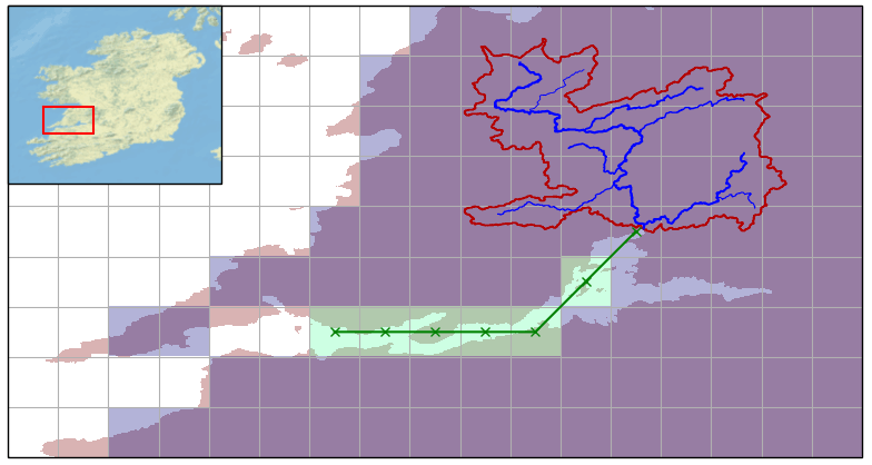
Figure 1 Example of an estuary opening: the red mask is the HR land mask, the blue mask is the 12D land mask, and the green mask represents the 12D cells converted from land to ocean to connect the river basin delineated in red to the ocean.

Using the land mask as a basis, the DRT algorithm is applied to upscale the MERIT-Hydro river network from 3 arcsec to $\mathrm{1}/\mathrm{12}$^∘ resolution. Details of the DRT algorithm may be found in Wu et al. (2011, 2012). The main steps are recalled below (Fig. 2 illustrates the process for the largest rivers of the Hérault basin in France):

1. Rivers are first sorted by decreasing flow accumulation at the outlet. Rivers are treated in this hierarchical order to ensure that the representation of large rivers is as good as possible. The following steps are applied for each river.

2. Given the river outlet, the HR river route is defined as the longest upstream river. The headwater cell is given by the first cell with a flow accumulation larger than a given threshold (10 % of the cell size, i.e. 1000 HR pixels).

3. The flow direction of the river at $\mathrm{1}/\mathrm{12}$^∘ is defined from the upstream cell to the outlet.

4. For each cell, the downstream cell is found when the HR route exits the cell with a minimum length (60 % of the cell size if cardinal, 80 % if diagonal; see e.g. cell C7 for river #2 in Fig. 2). Each time a flow direction is assigned, potential intersections are checked and corrected if necessary.

5. If a downstream cell is already assigned (e.g. by a larger river), the river is diverted: a parallel route is created that is as close to the real river as possible.

6. If the outlet is reached, the presence of loops is checked for and corrected if necessary, and the next largest river is treated (steps 2–6).

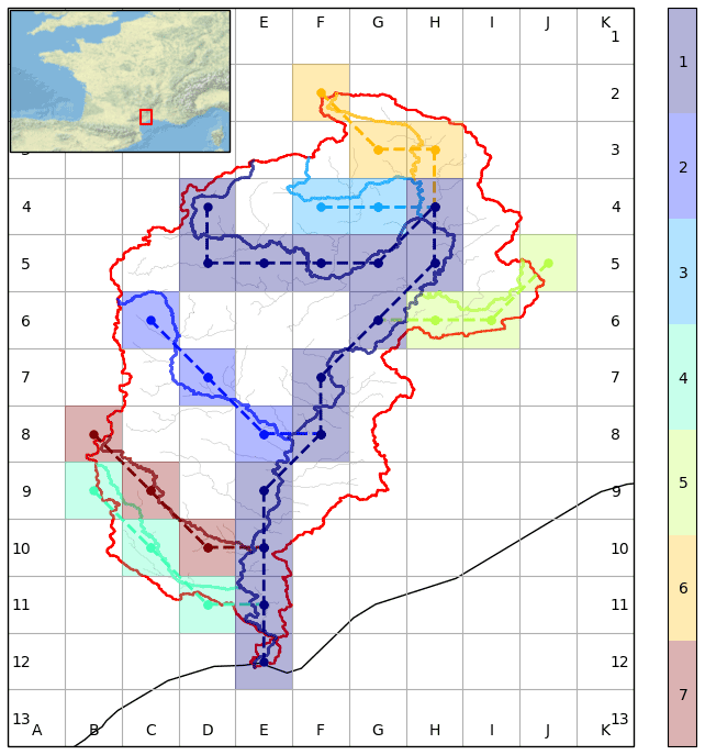
Figure 2 Example of network upscaling in the Hérault basin (France). Basin boundaries are drawn in red. Rivers are treated in descending order of drainage area and drawn with different colours; solid lines are used for HR and dashed lines for 12D.

River diversion (step 5) is an important feature of the algorithm as it allows the structure of the network to be conserved, but it simultaneously may raise problems with changes of river location (e.g. localization of gauge stations). To overcome this issue, it may be useful to keep a track of the relationship between HR and 12D rivers, which is done here by identifying each processed river with a unique id in both the HR and 12D networks. Note that while river diversion is necessary with the D8 convention, it can be avoided with the D∞ convention. Also, river diversion may have an impact on the attribution of input fluxes such as runoff that are used to force the routing model. However, we estimate that this impact can be neglected, as runoff is generally quite a smooth field at this resolution when modelled by a land surface model (LSM).

An example of diversion in the Loire River basin (France) is shown in Fig. 3. The Loire River (dark blue) is the major river of the Loire basin and is treated first. Second is the Vienne River (light blue), followed by the Cher River (green), the Creuse River (orange) and the Indre River (red). The cells M3 to H3 are occupied by the Loire River at 12D, so the Cher River portion within these cells has to be diverted to cells M4 to H4. Similarly, cells L4 to E4 are occupied by the Cher River and the Loire River at 12D, so the Indre River is diverted (to L5 to E5). River diversion allows us to conserve the river network structure as much as possible, even when several rivers flow within the same cell. Without diversion (e.g. river merging at cell M3), both gauge stations (green squares) in cell J3 would be associated with the Loire River, whereas one of them is actually located in the Cher River. River diversion allows us to conserve the locations of gauges as well as river nodes (confluences) within the river network tree.

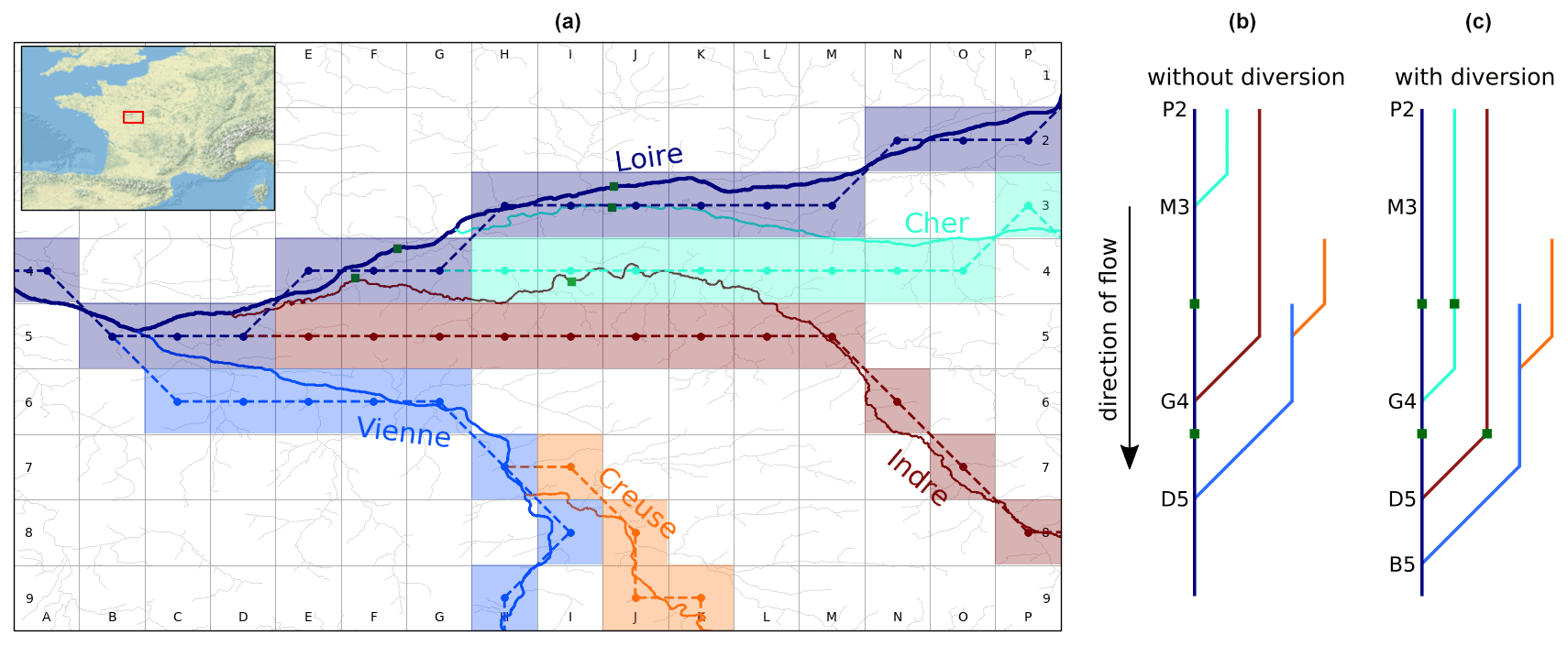
Figure 3 (a) Example of river diversions within the Loire River basin (France); (b, c) directional trees of the river network shown in (a). As in Fig. 2, rivers are treated in descending order of drainage area: (1) the Loire River (dark blue), (2) the Vienne River (light blue), (3) the Cher River (green), (4) the Creuse River (orange) and (5) the Indre River (red). Solid lines and dashed lines represent rivers at HR and 12D, respectively. Green squares represent gauge stations.

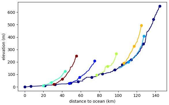
Hypsometry (elevation with respect to the longitudinal distance along the river) is computed during the process so that values of river length, slope and elevation are assigned to each cell at the end of the process. Figure 4 shows the hypsometry curves of the rivers shown in Fig. 2. Hypsometry is interpolated in the case of diversion. In addition, a unique identifier is assigned to each upscaled river and its corresponding river in the original HR network (as shown by colours in Figs. 2 and 3). This identifier and the hypsometry are used thereafter to derive the hydro-geomorphology parameters.

Figure 4 Examples of hypsometry curves for the rivers in Fig. 2.

The final river network at 12D at the global scale is represented in Fig. 5, and zooms over selected regions are provided in Fig. 6. For comparison purposes, Fig. S1 in the Supplement presents the river network over the same selected regions but at HD.

The type of river network required by most river routing models (especially those working with the D8 convention) has to provide a flow direction for each cell of the model. This ensures the closure of the global-scale water budget in earth system models. The type of soil (nature, river, lake, cities, etc.) and other characteristics (such as climate zone) are therefore not considered when setting up the global-scale river network. As a consequence, flow directions are also derived over arid regions where no river exists or within cells where no headwater stream has developed. In that sense, the river network should be considered a drainage network.

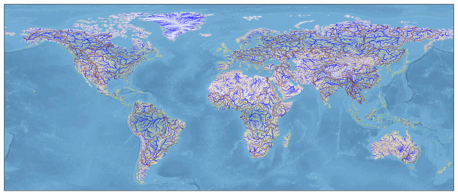
Figure 5 Global-scale river network at $\mathrm{1}/\mathrm{12}$^∘ resolution. The 69 largest basins in the world, which were used for the quality assessment, are delineated in brown.

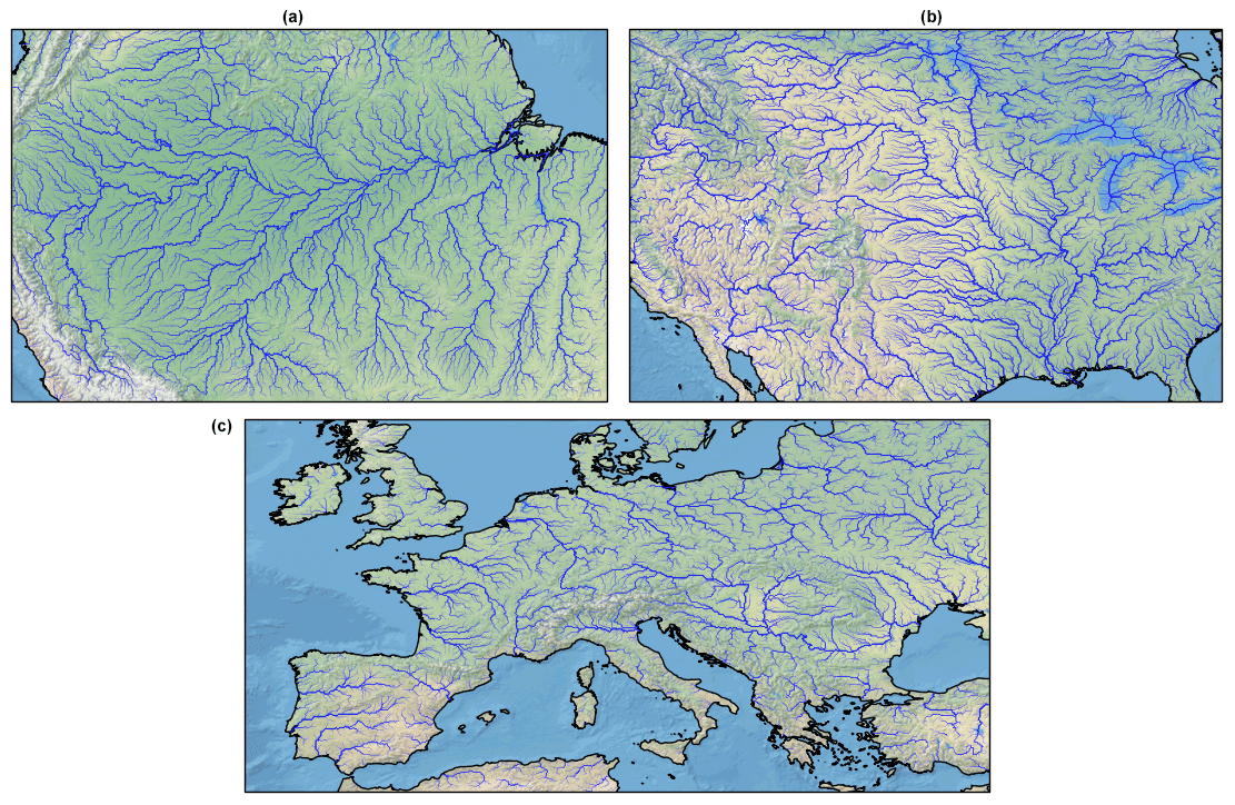
Figure 6 Regional-scale river network at $\mathrm{1}/\mathrm{12}$^∘ resolution: the Amazon basin (a), North America (b) and Europe (c).

2.3 Quality assessment

The DRT algorithm has been designed to conserve the river network structure as much as possible. The hierarchical river selection and river diversion have been set up for that purpose. The quality of the resulting river network has been assessed by Wu et al. (2011, 2012). Here, the 69 largest river basins (shown in Fig. 5) are assessed both qualitatively and quantitatively. Their total area equals 65.10⁶ km², which represents half of the total land area (excluding Antarctica and Greenland).

The qualitative assessment consists of visual comparisons of the river network from different sources, including the original MERIT-Hydro, the previous version of the CTRIP river network (CTRIP-HD) and Google Earth images. The boundary shapes of the basins have also been compared with those from CTRIP-HD, the original DRT network at 12D and the GRDC database (Lehner, 2012). For the latter, basin boundaries have been derived from the HydroSHEDS dataset at gauging stations within the 405 largest basins in the world. The basin boundary delineation has been carefully checked and is considered to be of high quality (Lehner, 2012).

The quantitative assessment first relies on the relative differences between the basin area from the newly developed 12D river network and those from other datasets, including the original DRT, MERIT-Hydro and GRDC. In addition, to assess the basin shape and coverage, an intersection-over-union (IoU) index is computed as

$$\begin{array}{}\text{(1)}& \text{IoU}=\mathrm{1}-{\displaystyle \frac{\text{area of the intersection basin mask}}{\text{area of the union basin mask}}}.\end{array}$$

The IoU index is applied on the basin masks computed from the new 12D network and the original DRT network. It equals 0 in the perfect case where the masks exactly overlap, and reaches 1 when the masks do not intersect. Details of the statistics are gathered in Table S1 in the Supplement.

Over the 69 largest basins, the overall agreement between MERIT-Hydro and the 12D river network is very good, with a median relative area difference of 0.3 %, which demonstrates the robustness of the upscaling algorithm. A large part of this difference can be attributed to basins crossing arid regions. When neglecting such basins, the mean relative difference drops from 5.8 % to 3.7 %. This cause of differences is discussed below.

Only two other basins are significantly different in the HR and 12D networks: those of the Nelson River and the Churchill River (Canada). Both river basins are connected via the South Indian Lake. The natural outlet of this lake flows into the Churchill River, but the lake is anthropized, and a part of the lake volume is diverted to the Nelson River basin for management purposes. The developer of MERIT-Hydro chose the Nelson River to be the major outlet of the South Indian Lake, considering the existing diversion project. We decided to disconnect this outlet, preferring to preserve the natural river network. Figure 7 zooms over the region surrounding the South Indian Lake. Yellow circles denote cells where the flow direction has been inverted to reconnect the lake to the Churchill River. Another noticeable difference can be seen for the Amur River basin (Asia), in which the Kherlen River appears disconnected to the Argun River, a tributary of the Amur River, while both are connected at Lake Hulun in the GRDC database. Lake Hulun is usually an inland lake without an outlet, but in wet periods it may overflow and then join the Argun River (Brutsaert and Sugita, 2008). As for the South Indian Lake, the developer of MERIT-Hydro preferred to keep them separated, which is reflected in the 12D river network (Fig. S2 in the Supplement).

Figure 7 Region surrounding the South India Lake in Canada where the river network has been corrected to follow the natural outlet of the lake to the Churchill River. Blue and red lines represent the river network at 12D and HR (MERIT-Hydro), respectively. The yellow line corresponds to the Nelson River and Churchill River delineation from GRDC. The yellow circles show the cells where the flow direction has been inverted to reconnect the lake to the Churchill River. The blue and red background masks correspond to the Nelson River and Churchill River basins extracted from MERIT-Hydro, respectively.

When compared to GRDC and DRT, the averaged relative area difference equals 5.6 % and 8.4 %, respectively. The median reaches 0.8 % in the comparison with DRT. This shows that, except for a few basins, the 12D river network and the original DRT are quite close. In Table S1, cells showing a relative area difference higher than 0.10 (10 %) are highlighted, and the potential cause of the difference is indicated by the background colour. Three main causes have been identified.

Most of the differences with GRDC and DRT come from the arid conditions characterizing parts of some basins (with a red background in Table S1). In such regions, the terrain is generally quite flat and often disconnected to the river network (endoreic). It is thus quite difficult to extract river networks, which explains the differences between the datasets (for example, within the basins of the Tigris–Euphrates and the Yellow, Senegal, Xi and Rufiji rivers). Nevertheless, the small amount of precipitation that can fall in such regions only partly infiltrates and is mostly evaporated. This volume of water never reaches the river network, so differences between river networks over arid regions can be neglected. This can be accounted for in the IoU index by removing arid regions from basin masks, with arid regions being defined as regions where the mean annual runoff is below a threshold fixed at 1 mm yr⁻¹. Figure 8 shows that the new 12D river network differs from GRDC in the southern part of the Tigris–Euphrates river system. Note that DRT is quite similar to GRDC in terms of basin delineation. This major difference can be neglected since it is within the arid region of the Arabian Peninsula. In most of the cases, the IoU significantly decreases (down to less than 10 %) when removing arid regions from the masks for basins that show large differences due to arid regions.

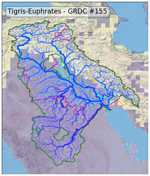
Figure 8 Tigris–Euphrates river system. River networks from the new algorithm and from DRT are drawn in blue and in cyan, respectively. Basin boundaries from the new algorithm, from DRT and from GRDC are drawn in green, magenta and orange, respectively. The overlapping blue mask represents arid regions. The IoU for this basin equals 14 %, which decreases to 8 % when the arid regions are removed.

Another source of differences is related to some missing tributaries (green background in Table S1 in the Supplement). This is the case for many river deltas, including those in the Tocantins, the Xi, the Ural, the Dvina and the Chao Phrava basins. With the D8 convention, models cannot simulate river divergence (a cell can flow into only one other cell). Figure 9 shows the case of the Red River, which joins the Mississippi Delta, but not in the main branch. This results in different river mouths in MERIT-Hydro and thus in the new 12D network.

The last noticeable difference is in the Neva River basin. It appears that in GRDC and DRT, Lake Saimaa (Finland) is disconnected from the Vuoksi River that flows into Lake Ladoga (Russia). As for the South Indian Lake, a significant part of the water is derived from Lake Saimaa to feed canals used for anthropogenic purposes (hydroelectricity, fluvial transport), which may reliably explain the disconnection of this sub-basin.

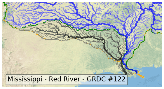
Figure 9 Lower Mississippi basin and Red River basin joining the Mississippi Delta. The Mississippi River network is drawn in blue and the Red River in black, while their boundaries are shown in green and grey, respectively. The orange line represents the basin boundary of the Mississippi River from GRDC.

Finally, the upscaling algorithm produced a reliable and consistent global river network at 12D that was very close to the GRDC database in terms of basin delineation for the 69 largest basins of the world. Since MERIT-DEM improved the HydroSHEDS high-resolution river network (Yamazaki et al., 2017), it is expected that the newly developed network improves the original DRT network.

3 Derivation of hydro-geomorphology parameters

Large-scale river routing models make use of a river network (flow direction) to propagate runoff within river basins to the oceans (in the case of exorheic basins). But the propagation dynamics also depends on geomorphological characteristics. These include river geometry (length, slope, width) and roughness (friction coefficient). For models that simulate floodplains, the topography (generally given as the relationships between the surface elevation, the area of the floodplain and the volume of water) is also needed, as well as the roughness in the floodplains. Similarly, when simulating the dynamics of groundwater and the exchanges with rivers, additional parameters are needed, such as soil porosity and transmissivity (or hydraulic conductivity). For large-scale models, floodplains and groundwater are usually simulated using a sub-grid approach, for example via a description of the distribution of the topography with respect to the elevation within each cell. This section describes the derivation of river parameters, as well as floodplain and groundwater sub-grid distributions, consistent with the river network derived in the previous section.

3.1 River parametrization

A set of parameters related to rivers and describing the flow dynamics within the river network are derived in this subsection.

For each cell, the river slope and bed elevation parameters are directly derived from the original MERIT-Hydro adjusted elevation during the upscaling of the river network by considering the river reach at HR associated with each 12D cell. It should be noted that applying DRT is quite similar to the vector‐grid‐hybrid method (Yamazaki et al., 2013) for the extraction of the ground elevation of each cell, except that the representative area of each pixel is computed not from the HR sub-catchment but directly from the HR river stretch within the cell. Nevertheless, given the type of model the current dataset is developed for (a simplified global-scale routing model), and given the uncertainties at this resolution in the runoff fields used to force the model, we suppose that the difference in area is negligible, at least for catchments covering several grid cells (or, equivalently, areas greater than 1000 km²).

For the river length within each cell, the computation relies on the HR route within the cell, contrary to other methods that use the flow direction to compute the distance between the centre of the cell and the centre of the following cell and then multiply this distance by a constant meandering ratio (e.g. CTRIP-HD). Here, meanders are accounted for in the computation of distances in the HR river route. The final river length within each cell is bounded between 1000 and 20 000 m. One may note that river reaches shorter than 1000 m correspond to headwaters, while reaches greater than 20 000 m correspond to highly meandering rivers. The river slope is also bounded between 10⁻⁴ m m⁻¹ in flat regions and 0.5 m m⁻¹ in mountainous areas.

The river width W_riv is mainly derived from the Global River Width from Landsat dataset (GRWL, Allen and Pavelsky, 2018; Frasson et al., 2019). The GRWL was developed by processing Landsat imagery at approximately mean annual flow. It provides high-resolution centreline locations alongside river widths for global rivers wider than 30 m. Water body type is given for each river reach as metadata. Here, reaches corresponding to a lake or reservoir, a canal or a tidally influenced river are discarded. Since the locations of river centrelines may not exactly match the river network at 12D, the river centrelines are first clipped in the MERIT-Hydro river network. Then the river identifier making the correspondence between HR and 12D is used to derive the river width for each cell at 12D (based on the median HR river width within each 12D cell). For grid cells where no river width can be derived from GRWL, we used the empirical relationship developed for previous versions of the CTRIP model (Vergnes et al., 2014), based on the annual mean discharge Q_mean:

$$\begin{array}{}\text{(2)}& W_{\mathrm{riv}}=\mathrm{5.41}{Q}_{\mathrm{mean}}^{\mathrm{0.59}}.\end{array}$$

Q_mean is derived from the runoff field in the GG-HYDRO database (Cogley, 2003) propagated through the river network. A threshold of 30 m is chosen as the minimum width. Figure 10 presents the distribution of river width from GRWL with respect to the annual mean discharge. It shows a strong relationship that is well captured by the empirical relationship from Vergnes et al. (2014).

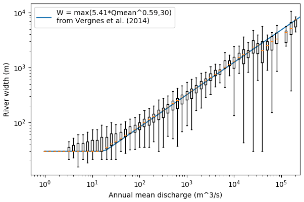
Figure 10 Distribution of river width from GRWL (Allen and Pavelsky, 2018) with respect to the annual mean discharge. The solid blue line represents the river width derived from the empirical relationship proposed by Vergnes et al. (2014).

Finally, smoothing is applied over each river (moving average with a 16-pixel width) to avoid unrealistic shrinkages (see Fig. 11).

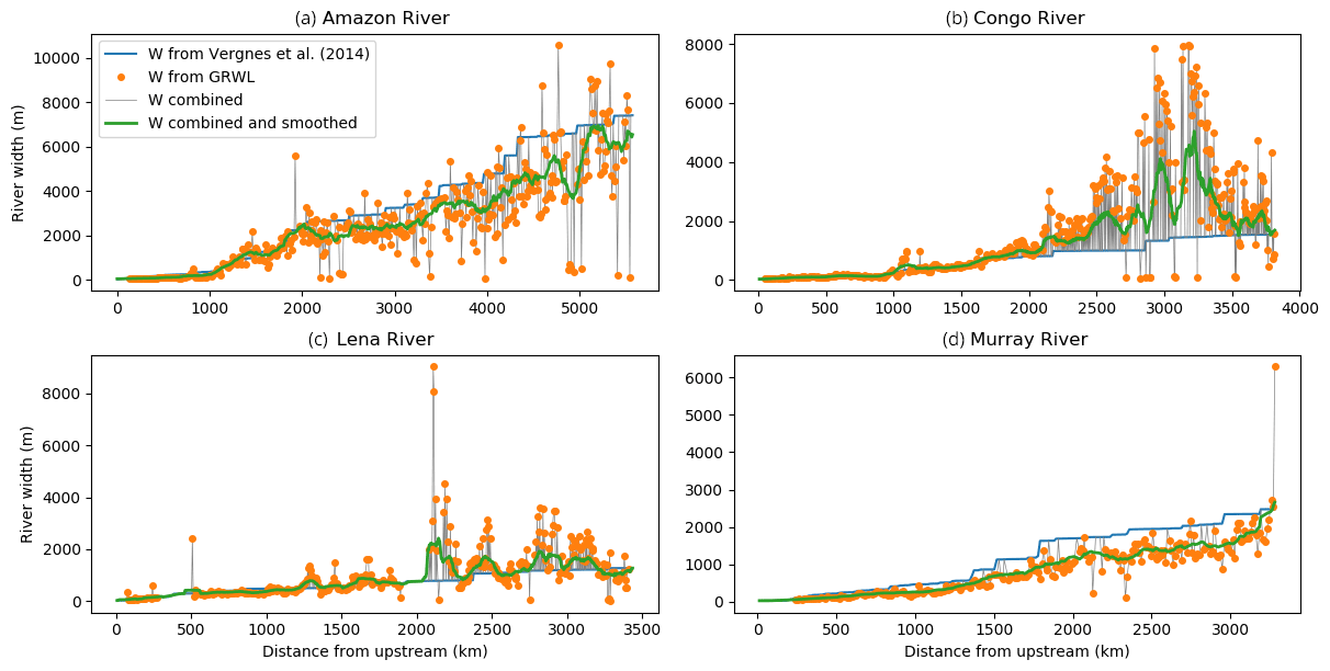
Figure 11 Examples of the combination of river widths from GRWL and Eq. (2) for (a) the Amazon River, (b) the Congo River, (c) the Lena River and (d) the Murray River.

The river depth h_riv (or bankfull depth), which is used to simulate floodplains, is derived from Eq. (3), as given in Decharme et al. (2019):

$$\begin{array}{}\text{(3)}& h_{\mathrm{riv}}=\mathrm{1.4}{W}_{\mathrm{riv}}^{\mathrm{0.28}}.\end{array}$$

The last parameter related to the river hydro-geomorphology is the roughness coefficient. Here, we used the same methodology as in Decharme et al. (2019). The roughness coefficient n_riv is derived from the weighted geometrical average of the value of 0.035 s m${}^{-\mathrm{1}/\mathrm{3}}$ (a standard value for quite large rivers, Lucas-Picher et al., 2003; Yamazaki et al., 2011) and the roughness coefficient n_fld describing the riparian zone and the vegetation in the surrounding potentially flooded area (described in the next section), where

$$\begin{array}{}\text{(4)}& n_{\mathrm{riv}}={\mathrm{0.035}}^{\mathrm{1}-{\mathit{\alpha }}_r}\times n_{\mathrm{fld}}^{{\mathit{\alpha }}_r}.\end{array}$$

The weighting coefficient α_r varies linearly from 1 in the headwater cells to 0.5 at the outlet of the river basin:

$$\begin{array}{}\text{(5)}& {\mathit{\alpha }}_r={\displaystyle \frac{\mathrm{1}}{\mathrm{2}}}\left({\displaystyle \frac{{\mathrm{SO}}_{max}-\mathrm{SO}}{{\mathrm{SO}}_{max}-{\mathrm{SO}}_{min}}}+\mathrm{1}\right),\end{array}$$

where SO is the stream order within the river basin and SO_min and SO_max are the minimum and maximum stream order values within the same basin, respectively.

Figure 12 shows the different parameters for different regions of the globe (the Amazon basin, the USA and Europe).

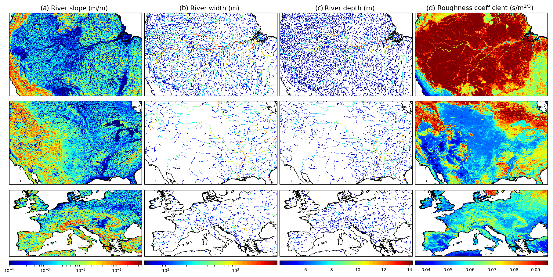
Figure 12 River parameters for the Amazon (first row), the USA (second row) and Europe (third row): river slope (a), river width (b), river depth (c) and roughness coefficient (d). River widths smaller than 50 m and river depths smaller than 4 m have been filtered out for clarity.

3.2 Floodplain parametrization

Floods may occur when the water height within the river exceeds the river depth, causing lateral flows over the river banks. A floodplain, described as an area surrounding a river that can be flooded during heavy rain events, provides water storage and directly impacts the water propagation within the river network. High-accuracy representation of the flow dynamics within floodplains requires a highly accurate DEM and intensive computations to solve the 2D Saint-Venant equations. This can be done over small areas, such as urban areas, but not at regional scales. A number of large-scale river models that account for floodplains and their impacts on the flow dynamics are based on sub-grid approximations (Yamazaki et al., 2011; Decharme et al., 2012). This concept generally relies on computing the volume of water that flows outside the river (given the river maximum volume) and estimating the water level and the area of the flooded zone from sub-grid distributions (Decharme et al., 2012).

Here, in order to ensure consistency between the river network and the floodplain representation, the adjusted elevation from MERIT-Hydro is used as the baseline to compute the sub-grid distributions of elevation, cell fraction (related to the area) and volume of water within the floodplain. The method used to extract these distributions is described in Decharme et al. (2012).

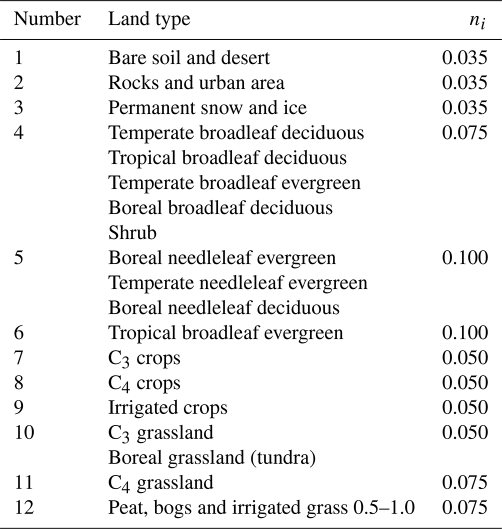
The floodplain roughness is used to estimate the flow velocity between the river and the floodplain, using the Manning–Strickler equation. In addition, a floodplain roughness coefficient is estimated empirically as in Decharme et al. (2019). This coefficient is directly related to the type of land within the cell. The ECOCLIMAP-II land cover database (Faroux et al., 2013) was used to characterize the type of land. For each cell at $\mathrm{1}/\mathrm{12}$^∘, we computed the fraction f_i of each land type listed in Table 1. Then the floodplain roughness was computed as the weighted average of the default values n_i for each land type (as given in Table 1):

$$\begin{array}{}\text{(6)}& n_{\mathrm{fld}}=\sum _{i=\mathrm{1}}^{\mathrm{12}}\left(f_i\times n_i\right).\end{array}$$

Table 1 The 12 land types derived from the 1 km ECOCLIMAP-II database and their corresponding Manning roughness values.

3.3 Groundwater parametrization

Like floodplains, aquifers can significantly impact the propagation of water within rivers. Aquifers are usually recharged by the infiltration of water at the surface and can interact directly with rivers. The direction of the exchange between a river and an aquifer depends on the water elevation in the river and the water table depth. Just as for floodplains, some large-scale hydrology models (e.g. Döll and Fiedler, 2008; Vergnes and Decharme, 2012; Decharme et al., 2019) integrate a simplified representation of aquifers in order to better represent the continental water cycle and, more specifically, the water propagation within the river network.

To delineate the main aquifers that could be represented in large-scale hydrology models, Vergnes and Decharme (2012) used the global map from the Worldwide Hydrogeological Mapping and Assessment Programme (WHYMAP; http://www.whymap.org, last access: May 2022). As in Vergnes and Decharme (2012), we considered two of the three categories included in this map for which the two-dimensional diffusive solver is well adapted: the “major groundwater basin” that gathers sedimentary basins and the alluvial plains with permeable materials, and the “complex hydrogeological structure”, which includes (among others) alluvial aquifers formed by the deposition of weathered materials. The “local and shallow aquifers” category corresponds to the old geological platforms characterized by crystalline rocks with scattered, superficial aquifers, and is not considered here. Finally, mountainous cells were removed by using a criterion on terrain slopes, and the global lithology map from Dürr et al. (2005) was used to refine the delineation of aquifers. Examples of aquifer delineation are shown in Fig. 13a.

In Vergnes and Decharme (2012), the groundwater dynamics is described by a two-dimensional diffusive equation that requires some additional parameters characterizing the soil, such as the effective porosity and the transmissivity. These characteristics highly depend on the lithology and can be estimated from mean values in the literature. Here, the lithology was derived from Dürr et al. (2005) and the mean values were from Table 1 in Vergnes and Decharme (2012). Note that values of porosity and transmissivity have been capped at 0.05 m³ m⁻³ and 0.02 m² s⁻¹, respectively, in order to avoid excessive inertia within the corresponding aquifers. Values of both parameters for different regions of the globe are shown in Fig. 13b–c.

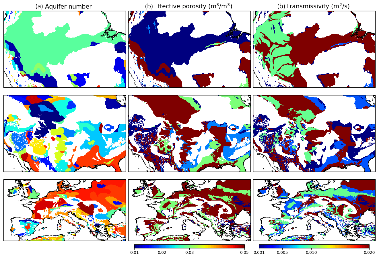
Figure 13 Aquifer numbering and parameters for the Amazon (first row), the USA (second row) and Europe (third row): aquifer number (a), effective porosity (b) and transmissivity (c).

Lastly, to simulate the exchanges between aquifers and rivers, the piezometric head has to be simulated and compared to the water level within the river. The piezometric head may be also used to represent upward capillary fluxes to the vegetation root layer (Vergnes et al., 2014). Just as for floodplains, a sub-grid approach may be used, as in Vergnes et al. (2014) and Decharme et al. (2019), to derive the distribution of the elevation and the cell fraction within each cell. Here again, the adjusted elevation from MERIT-Hydro is used to compute these distributions.

4 Validation

4.1 Modelling configuration

In this section, we set up a model configuration with the river network and the parameters described in Sects. 2 and 3. For this validation step, the CTRIP model is used with the same configuration as in Decharme et al. (2019). In the latter study, CTRIP is operated at 0.5^∘ resolution (CTRIP-HD) and the groundwater and floodplain components are accounted for. CTRIP-HD has been extensively validated against various types of observations, including river discharge, flood extent, groundwater head and total water storage (Alkama et al., 2010; Decharme et al., 2012, 2019; Vergnes and Decharme, 2012; Vergnes et al., 2014). The whole set of hydro-geomorphological parameters derived in this paper at 12D are available for CTRIP-HD. Consequently, the 12D set of parameters can be evaluated and compared to the HD set of parameters while keeping a consistent modelling framework.

Both configurations are forced by runoff and drainage fields generated by the ISBA land surface model, as described in Decharme et al. (2019). The atmospheric forcings applied to ISBA are the Earth2Observe (E2O) dataset. Although the ISBA and CTRIP models are fully coupled in Decharme et al. (2019), we prefer to run the CTRIP model in offline mode here; then, the configuration considered here includes the representation of floodplains and aquifers, but backward fluxes to ISBA (capillary rise and evaporation over floodplains) are neglected. The half-degree runoff and drainage fields are downscaled at 12D with a simple nearest-neighbour method and provided to the CTRIP model in daily time steps over the period 1979–2014. The CTRIP simulation time step is set at 3600 s, and the time step for output river discharge is 24 h (daily). Finally, a 30-year spinup period was used to let the groundwater storage state variable reach its equilibrium value.

4.2 Evaluation strategy

Here we compare the performance of the new configuration (CTRIP-12D) to that of the previous one (CTRIP-HD). The performance mainly relies on comparisons between simulated and observed discharges at more than 10 000 in situ gauge stations over the globe.

4.2.1 River discharge datasets

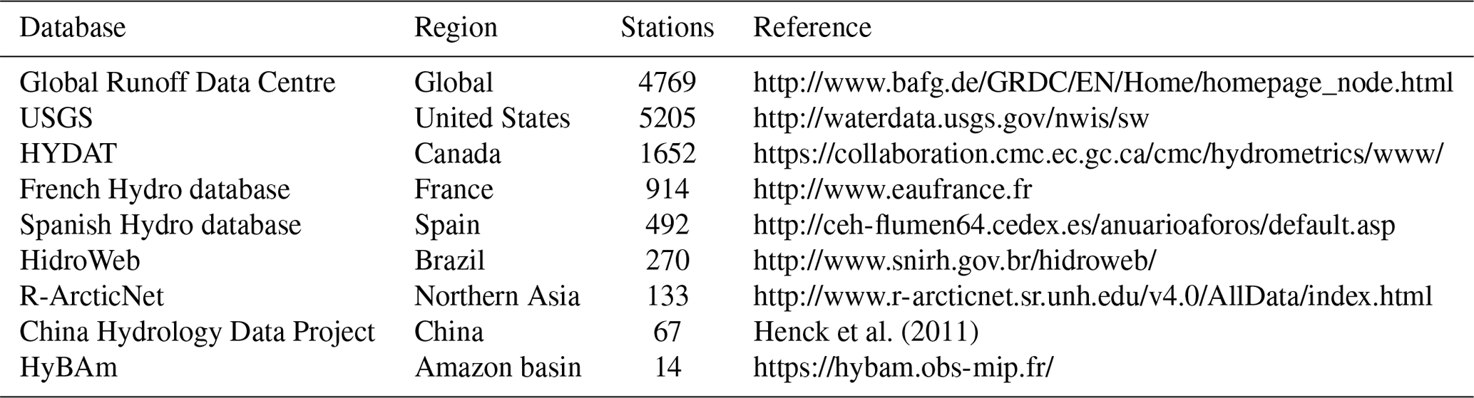
A large number of in situ gauge stations have been considered for the comparison with simulated discharge. The data were extracted from various open-access databases described in Table 2. A minimum of 3 years of records from the period 1979–2014 were imposed as a mandatory criterion, as well as the presence of localization and drainage area in the station metadata. A total of 13 516 stations were finally selected, with drainage areas ranging from 400 to 4.7×10⁶ km².

Henck et al. (2011)

Table 2 Description of the databases considered for the selection of in situ gauge stations with at least 3 years of discharge observations within the period 1979–2014. All websites were last accessed on 25 February 2021.

4.2.2 Localization of gauge stations

For the comparison between observed and simulated discharges, one must first localize the gauge station within the river network of the model. A very common method of achieving this consists of looking for the grid pixel around the station for which the drainage area is the closest to the one reported in the station metadata. However, in some cases, this can lead to the erroneous selection of the CTRIP pixel corresponding to a certain station. Such problems can happen unwittingly (see the example in Fig. 14) or for portions of rivers that have been diverted during the generation process (Sect. 2). This highlights the necessity to improve the localization methodology.

Since the coordinates and the drainage area of each station are known, it is possible to delineate the catchment related to the station from the MERIT-Hydro database. First, the pixel in the HR grid corresponding to the station is designated by selecting the pixel that minimizes a criterion that combines the distance to the station and the drainage area. At such a high resolution, the method can be considered robust enough to avoid mislocalization.

The second step consists of sorting the CTRIP pixels around the station (as in Fig. 14) in order of descending drainage area. For each pixel, the comparison between the catchment delineation obtained from MERIT-Hydro and that from CTRIP is quantified by computing the IoU index (Eq. 1). Finally, the relative error in the area (a_cost) and the relative error in the mask overlap (m_cost) are combined to find the best candidate.

Consequently, each station is assigned a CTRIP pixel more consistently than when using classical approaches. This process is applied for CTRIP-HD and CTRIP-12D. It also ensures that basins smaller than one grid pixel are excluded from the selection, since m_cost would be too high. Note also that the method is able to solve potential localization difficulties due to the river diversion allowed during the network generation process (Section 2). Although river diversion can foster this kind of situation, at the same time it allows the correct localization of the confluences within the network. This avoids artificial confluences and consequently prevents the stations concerned from being discarded (due to a bad mask overlap).

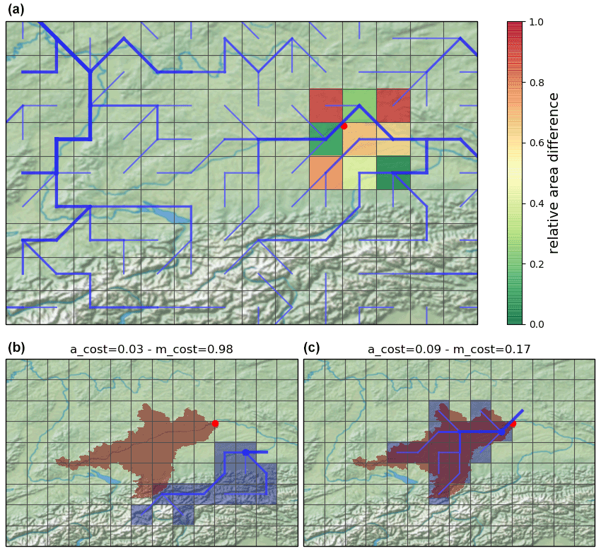
Figure 14 Example of necessary relocalization using the mask overlapping method. The station (red dot) is the Oberndorf station (GRDC id 6342910) on the Danube River (48.947^∘ N, 12.0149^∘ E). In the two lower panels, the real basin (from MERIT-Hydro) is shown in red. The lower left panel shows the CTRIP basin (in blue) for the cell with the drainage area closest to the drainage area reported at the station (i.e. the relative error in the area a_cost is the lowest). The lower right panel shows the CTRIP basin for the cell with the lowest relative error in the mask overlap (m_cost).

4.2.3 Evaluation metrics

The main metric used to quantify the performance of each simulation is the modified Kling–Gupta efficiency (KGE, Kling et al., 2012). The KGE is a combination of three factors describing the error: the relative bias, correlation and relative variability (Eq. 7). The KGE varies from −∞ to 1 (the upper bound corresponding to simulation results that perfectly match the observations) and is given by

$$\begin{array}{}\text{(7)}& \text{KGE}=\mathrm{1}-\sqrt{(r-\mathrm{1}{)}^{\mathrm{2}}+(\mathit{\beta }-\mathrm{1}{)}^{\mathrm{2}}+(\mathit{\gamma }-\mathrm{1}{)}^{\mathrm{2}}}\end{array}$$

$$\begin{array}{ll}{\displaystyle }\mathit{\beta }& {\displaystyle }={\displaystyle \frac{{\mathit{\mu }}_s}{{\mathit{\mu }}_o}}\\ {\displaystyle }\mathit{\gamma }& {\displaystyle }={\displaystyle \frac{{\mathit{\sigma }}_s/{\mathit{\mu }}_s}{{\mathit{\sigma }}_o/{\mathit{\mu }}_o}},\end{array}$$

where r is the correlation coefficient between simulated and observed discharges, β is the bias ratio, γ is the variability ratio, μ is the mean discharge and σ is the standard deviation.

We also use the normalized information contribution (NIC), which is particularly suited to quantifying the improvement between two simulations, as in Albergel et al. (2018):

$$\begin{array}{}\text{(8)}& \text{NIC}={\displaystyle \frac{{\text{KGE}}_{\text{new}}-{\text{KGE}}_{\text{ref}}}{\mathrm{1}-{\text{KGE}}_{\text{ref}}}},\end{array}$$

where KGE_ref is the KGE criterion for the reference simulation and KGE_new is the KGE criterion for the simulation that is compared to the reference. The advantage of the NIC criterion is that it normalizes the difference between the KGEs of two experiments. The impact of a given KGE difference on performance depends on the KGE values. For instance, if KGE_ref=0 and KGE_new=0.2 then NIC =0.2, whereas if KGE_ref=0.8 and KGE_new=1 then NIC =1. The higher NIC value in the second case means that the improvement is better (perfect in that case), even though the difference in KGE is the same.

4.3 Simulation performance

4.3.1 Evaluation of CTRIP-12D

In this section, the modelling results are evaluated by comparing simulated and observed river discharges at the 13 516 gauge stations selected from various open-access databases, as described in Sect. 4.2.1.

Figure 15 shows the KGE values for the 11 238 stations with a KGE greater than −1 (the others have been discarded from this figure for the sake of clarity) and zooms over the Amazon basin, North America and Europe. Globally, the CTRIP-12D model clearly shows quite good performance whatever the basin area, especially in South America, Europe, South-East Asia and the eastern part of the USA. The KGE decreases when the CTRIP-12D model is unable to satisfactorily reproduce the river discharge. Among all the stations, 2278 show a KGE lower than −1, which corresponds to very poor performance. Nevertheless, it has to be noted that most of these stations have a quite small drainage area (90 % have a drainage area smaller than 50 000 km²; 75 % have a drainage area smaller than 10 000 km²). Different reasons have been identified that can explain such deficiencies. First, some rivers are highly regulated, which is not accounted for here. Second, in some regions, the ISBA land surface model may fail to produce realistic runoff (which is used to feed CTRIP) because of model and atmospheric uncertainties (e.g. in mountainous areas). Third, in arid regions (e.g. in the Niger basin), the evaporation over open waters (rivers and floodplains) can be very high but is not accounted for here, which greatly impacts the discharge ratio. Finally, the dynamics of lakes is neglected, which also impacts the quality of the results, mainly in terms of the correlation and standard deviation.

To verify that poor performance is mainly due to these reasons and not to the new parametrization at 12D, the next section compares the performance of CTRIP-12D with that of CTRIP-HD when both are run in the same configuration.

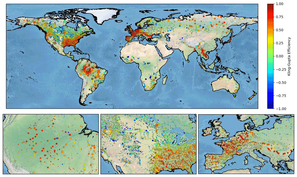
Figure 15 Kling–Gupta efficiency for CTRIP-12D over 11 238 gauge stations (with KGE $>-\mathrm{1}$), and zooms over the Amazon basin, North America and Europe. The circle size depends on the drainage area at the station.

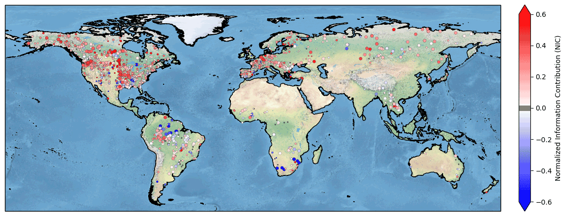
Figure 16 NIC of the Kling–Gupta efficiency between CTRIP-12D and CTRIP-HD over 2164 gauge stations (with KGE $>-\mathrm{1}$). The circle size depends on the drainage area at the station.

4.3.2 Comparison with CTRIP-HD

Considering that the CTRIP-HD model in its current version has been extensively validated (e.g. Alkama et al., 2010; Decharme et al., 2012; Vergnes and Decharme, 2012; Vergnes et al., 2014; Decharme et al., 2019), we mainly focus on the comparison between this version of CTRIP and the new one at 12D developed in this article.

Figure 17 Panels (a, c, e) show the distributions of the KGE (a), correlation r (c) and γ coefficient (e) with respect to the drainage area at each station for both CTRIP-HD and CTRIP-12D (numbers above the boxes represent the number of stations within each area bin). Panels (b, d, f) show the cumulative density function of the KGE (b) and the probability density functions of the correlation r (d) and γ coefficient (f).

By applying the methodology to localize gauge stations within the river network (see Sect. 4.2.2), 2612 stations were selected as having the correct localization in the river networks of both CTRIP-HD and CTRIP-12D. For those stations, we computed the KGE values for both simulations as well as the NIC criterion, which quantifies the improvement or degradation of CTRIP-12D compared to CTRIP-HD. As written in the previous section, despite the overall good quality of the CTRIP model, it may fail to reproduce observed discharges, in particular for stations that are highly influenced by human activities, which are not represented in CTRIP. We consider that the CTRIP model is not adapted for those stations due to the presence of processes that are not accounted for. Consequently, we consider that the improvement or degradation of model performance is not relevant for those stations and we discard them. Figure 16 presents the NIC values for all the stations with KGE values greater than −1 (2164 stations). It shows that performance is generally better with the new resolution. More precisely, 1988 stations (92 %) are impacted by the new parametrization (|NIC$|>\mathrm{0}$.02), including river routing (river network and parameters), floodplains (roughness and sub-grid topography) and groundwater (aquifer parameters and sub-grid topography). Among those stations, 470 (24 %) are negatively impacted, while 1518 (76 %) are positively impacted.

To get a closer look at the difference in performance between CTRIP-HD and CTRIP-12D, panels in Fig. 17 show the distributions of the KGE, correlation and γ variability coefficient for both simulations. For each criterion, the left panel (a, c, e) shows the criterion with respect to the drainage area at the gauge station. For this comparison, no station with a drainage area smaller than 1000 km ² has been selected because of the low resolution of CTRIP-HD. Whatever the resolution, the KGE and correlation increase with the drainage area, but for both criteria, performance is clearly better for CTRIP-12D for all categories of drainage area. A similar result is seen for the relative variability depicted by γ in Fig. 17e, as median and quartile values are closer to 1 for CTRIP-12D. The right panels (b, d, f) of Fig. 17 also show an overall better performance for CTRIP-12D in terms of KGE and correlation and because the γ distribution is closer to 1.

Better performance could be expected for smaller basins, since these basins are represented by just a few cells at HD, and the difference between the basin delineation at HD and 12D could be relatively high, leading to different contributing areas. The better performance of CTRIP-12D for larger basins is less expected. Indeed, the processes and forcing are the same for both configurations, and the parameters are derived using similar strategies and relationships. The improvement in the correlation and variability demonstrates that a better-defined river network improves the dynamics of river propagation within the basin and interactions with floodplains and aquifers. Other potential sources of differences between the models include (1) the reference HR dataset (HydroSHEDS for CTRIP-HD, MERIT-Hydro for CTRIP-12D), which impacts the generation of floodplain and aquifer sub-grid parametrization, and (2) the use of observation-based river widths for CTRIP-12D.

5 Code and data availability

The river network and hydro-geomorphology datasets (including the floodplain and aquifer parametrizations) are freely available for download from Zenodo (https://doi.org/10.5281/zenodo.6482906, Munier and Decharme, 2022). The source code is also available in this repository.

6 Conclusions

This article has presented a new global-scale river network at $\mathrm{1}/\mathrm{12}$^∘ (12D) derived from the MERIT-Hydro high-resolution hydrography data. We have also provided a set of hydro-geomorphological parameters that are consistent with this new river network. The set of parameters includes length, width, depth and roughness for rivers, roughness and sub-grid topography for floodplains, and transmissivity, effective porosity and sub-grid topography for aquifers.

The new river network and hydro-geomorphological parameters have been implemented in a new version of the CTRIP model (Decharme et al., 2019) and assessed through a simulation performance comparison with the previous version of CTRIP at 1/2^∘ (HD). It was shown that, overall, river discharges are better estimated with the 12D version, and the improvement can be mainly attributed to the finer representation of the real river network. When increasing the resolution of CTRIP from HD to 12D, the total number of cells changes from 62×10³ to 2.2×10⁶, the total number of basins increases from 4800 to 56 500, and the total river length increases from 2.5×10⁶ to 21×10⁶ km.

For perspective, it should be mentioned that the derivation of some parameters for some regions could be improved by using existing local or national data. For example, aquifers could be better described by the Référentiel Hydrogéologique Français (BDRHF) database available for France, or by hydrogeological maps from USGS for the United States.

In grid-based approaches, the river network is discretized on a regular Cartesian grid, so that unit catchments are rectangular pixels with their own hydrogeomorphological characteristics. The complete dataset described here is particularly well suited to a number of large-scale RRMs that use a gridded structure for global hydrological studies (see Table 2 in Kauffeldt et al., 2016). Not all of them are currently running at 12D resolution; on the other hand, the current tendency suggests that 5 arcmin could become the next standard resolution for global-scale climate studies, namely via the recent release of the last global meteorological dataset for impact models in phase 3a of the Inter-Sectoral Impact Model Intercomparison Project (ISIMIP3a Dirk et al., 2022). With the entire dataset described here (flow direction, river length, river slope, river bankfull depth, river roughness, floodplain roughness, major groundwater basin boundaries, aquifer transmissivity and aquifer effective porosity), many hydrological models could improve their river routing module by increasing the spatial resolution. Moreover, this consistent and comprehensive dataset can help modellers to integrate some important processes (such as inundation and groundwater) that are still neglected in some models.