the Creative Commons Attribution 4.0 License.
the Creative Commons Attribution 4.0 License.
 | 05 May 2022
Observations of the lower atmosphere from the 2021 WiscoDISCO campaign
Gijs de Boer
Joseph P. Hupy
Steven Borenstein
Jonathan Hamilton
Ben Kies
Dale Lawrence
R. Bradley Pierce
Joe Tirado
Aidan Voon
Timothy Wagner
The mesoscale meteorology of lake breezes along Lake Michigan impacts local observations of high-ozone events. Previous manned aircraft and UAS observations have demonstrated non-uniform ozone concentrations within and above the marine layer over water and within shoreline environments. During the 2021 Wisconsin's Dynamic Influence of Shoreline Circulations on Ozone (WiscoDISCO-21) campaign, two UAS platforms, a fixed-wing (University of Colorado RAAVEN) and a multirotor (Purdue University DJI M210), were used simultaneously to capture lake breeze during forecasted high-ozone events at Chiwaukee Prairie State Natural Area in southeastern Wisconsin from 21–26 May 2021. The RAAVEN platform (data DOI: https://doi.org/10.5281/zenodo.5142491, de Boer et al., 2021) measured temperature, humidity, and 3-D winds during 2 h flights following two separate flight patterns up to three times per day at altitudes reaching 500 m above ground level (a.g.l.). The M210 platform (data DOI: https://doi.org/10.5281/zenodo.5160346, Cleary et al., 2021a) measured vertical profiles of temperature, humidity, and ozone during 15 min flights up to six times per day at altitudes reaching 120 ma.g.l. near a Wisconsin DNR ground monitoring station (AIRS ID: 55-059-0019). This campaign was conducted in conjunction with the Enhanced Ozone Monitoring plan from the Wisconsin DNR that included Doppler lidar wind profiler observations at the site (data DOI: https://doi.org/10.5281/zenodo.5213039, Cleary et al., 2021b).
- Article
(7413 KB) - Full-text XML
- BibTeX
- EndNote


WiscoDISCO-21 (Wisconsin's Dynamic Influence on Shoreline Circulations on Ozone) was designed to capture lake breeze influence on the shoreline ozone observations and to interrogate the low-altitude dimensionality of the marine layer as it moves on shore. The lake breeze is a mesoscale phenomenon driven by differential air temperatures over land and water surfaces, which in spring and early summer produces a solenoidal circulation in a baroclinic environment that manifests itself as onshore flow during the day. A strong inversion develops as a shallow layer of maritime air is advected onshore and displaces the warmer terrestrial air upward (Holton, 1992; Miller et al., 2003; Martin, 2006; Wagner et al., 2022). These circulations can act as a transport mechanism of emissions on land to over water at night and in early morning hours, then allowing those emissions to not mix when trapped in cooler temperature-inverted air masses over water, eventually being driven back on land through a lake breeze. The goals of the campaign were to (a) characterize lake breeze characteristics of nearshore circulation onset and vertical shape along the shoreline of Lake Michigan, (b) capture the development or movement of convergence zones/fine-scale circulations within the lake-breeze frontal region from offshore to onshore over time, and (c) monitor ozone gradients, characteristics of chemical circulation patterns within marine-influenced inversions at the shoreline at low altitudes.
The influence of lake breeze on shoreline air quality along Lake Michigan (Keen and Lyons, 1978; Lyons and Cole, 1976; Lyons and Olsson, 1973; Dye et al., 1995; Foley et al., 2011; Stanier et al., 2021) and other Great Lakes (Hayden et al., 2011; Levy et al., 2010; Wentworth et al., 2015; Sills et al., 2011) is well documented by campaigns incorporating ground (Lyons and Cole, 1976), ferry (Lennartson and Schwartz, 2002; Cleary et al., 2015), and aircraft observations (Dye et al., 1995; Foley et al., 2011; Hayden et al., 2011; Stanier et al., 2021). The shoreline communities of Lake Michigan have historically been in non-attainment of federal ozone standards. Precursors to ozone production, volatile organic compounds (VOCs) and nitrogen oxides (NOx), have emission sources along the Chicago urban corridor, and ozone production can be enhanced when those emissions are trapped in the marine layer over the lake and get transported northward from Chicago (Vermeuel et al., 2019; Dye et al., 1995; Foley et al., 2011). The low-altitude features in ozone gradients over Lake Michigan have been observed in the recent 2017 Lake Michigan Ozone Study field campaign (Stanier et al., 2021; Doak et al., 2021). Stanier et al. (2021) describe observations for the highest measured ozone during the field campaign existing over water, offshore from Milwaukee and in the altitude range of 30–100 m above lake level. Air quality models have been shown to inadequately represent overwater ozone (Cleary et al., 2015; McNider et al., 2018; Qin et al., 2019) and do not always capture the ozone gradients at the shoreline (Stanier et al., 2021; Abdi-Oskouei et al., 2020). The shallow marine layer disruption when crossing a shoreline boundary during a lake breeze is a unique environment to study the changes in vertical mixing and pollutant extent.
WiscoDISCO-21 featured round-based Doppler lidar observations and two uncrewed aircraft systems (UASs), including the University of Colorado RAAVEN fixed-wing UAS and Purdue University's DJI M210 quadcopter. These platforms were deployed to enhance the level of detail and extend the domains of ground-based measurements to manned aircraft observations with higher spatial resolution and sustained lower-altitude flight. UASs are well suited to make observations of a shoreline environment impacted by a shallow marine layer, where vertical mixing and pollutant transport are key to understanding pollution events at the surface. UASs have been used in riverine environments to highlight pollutant transport and nighttime boundary layer dynamics (Guimaras et al., 2020). During the Ozone Water-Land Environmental Transition Study (OWLETs), UASs, ozone sondes, and lidar observations were used to observe ozone titration events above the Chesapeake Bay shipping channel (Gronoff et al., 2019). Horel et al. (2016) describe the use of distributed ground sensors, tethered sondes, and UASs to better understand the meteorological and pollutant transport factors surrounding poor air quality in the Salt Lake valley. The incorporation of multi-hole probes into fixed-wing UASs has allowed for observations of 3-D winds (Elston et al., 2015) and turbulent fluxes (Wildmann et al., 2014). The RAAVEN platform leveraged in WiscoDISCO-21 has recently been used to study the lower atmosphere across a variety of environmental regimes. This includes nearly a month of flight operations to investigate the thermodynamic and kinematic structure of trade winds over the tropical Atlantic Ocean (de Boer et al., 2022a) as well as deployments to the US Midwest to make measurements of supercell thunderstorms (Frew et al., 2020). The measurement accuracy of the RAAVEN's instrumentation was recently evaluated at the US Department of Energy's Atmospheric Radiation Measurement (ARM) program's Southern Great Plains facility (see de Boer et al., 2022b, for details).
Such high-resolution UAS observations are well-suited for documenting and characterizing the dimensions of the lake breeze phenomenon and corresponding pollutant transport. A combination of UASs and lidar can provide overlapping domains of observations that scale up to the planetary boundary layer, with UASs providing detailed insight into nonuniformities in meteorological observations along the Lake Michigan shoreline. UAS observations are particularly complementary to Doppler lidar observations, as such observations are subject to near-field issues that prevent them from making observations at very low altitudes. Given that the UASs readily operate between the surface and 100 m, these platforms can fill in this gap and provide detailed insight into thermodynamic, kinematic, and chemical properties of this layer. These observations have higher vertical and temporal resolution than many chemical models, which can provide insight into model resolution issues at the lake–land interface (Wagner et al., 2022). The WiscoDISCO-21 field campaign was conducted in conjunction with the Enhanced Ozone Monitoring initiative from the Wisconsin DNR who housed added instrumentation for NO, NOx (NOx= NO + NO2), NOy (NOy is the sum of all reactive nitrogen species), VOC canisters, and PANDORA instrumentation at the Chiwaukee Prairie air monitoring station. The NO, NOx, and VOC measurements can give some indication of the availability of precursors for ozone production and NOy measurements, and some specific VOCs can indicate something about the past ozone production history of an air parcel. The Wisconsin DNR has provided a portal for access to data from these sensors through their web portal (https://wi-dnr.widencollective.com/portals/iwvftorq/AirMonitoringData, last access: 21 April 2022).
These datasets can be used in a variety of ways to better understand the meteorology and pollution episodes at the Lake Michigan shoreline. The lidar WindPRO data and RAAVEN data provide complete coverage of the atmospheric dynamics of the marine layer such that it can be characterized and modeled (Wagner et al., 2022; Jozef et al., 2022). Those characterizations could be used to test the fidelity of operational meteorological models (such as HRRR) in modeling the stable boundary layer height. The datasets can also be used to test models for the roughness parameterizations in a shoreline environment using overwater and overland turbulence. The combination of ozone data with the meteorological data can be used to constrain air quality models for the chosen mixing volume for chemical processing in the atmosphere, using the FOAM model (Vermeuel et al., 2019) or testing vertical grid-scale sizing of nested high-resolution models for their ability to reproduce the gradients in ozone as measured using UASs (Abdi-Oskouei et al., 2020). The lake breeze phenomenon is similar to bay breeze and sea breeze circulations that complicate modeling efforts in other shoreline locations impacted by poor air quality (Caicedo et al., 2021; Geddes et al., 2021), and model fidelity is crucial to the development of appropriate emissions controls in these environments.
2.1 University of Colorado RAAVEN UAS
The RAAVEN UAS (Fig. 1) is a fixed-wing UAS with a wingspan of 2.3 m that has been operated by the University of Colorado Boulder since 2019. The RAAVEN's airframe is based on a custom-manufactured model from RiteWing RC. The airframe has been updated to meet the needs of atmospheric science missions spanning a variety of environments. The RAAVEN leverages the PixHawk2 autopilot system and employs an 8S 21 000 mAh lithium ion (Li-Ion) battery pack to offer flight times around 2.5 h, depending on conditions and executed flight patterns. Specific modifications to the airframe include the integration of a tail boom to enhance longitudinal stability and improve the platform's performance. The aircraft has a top airspeed of approximately 130 km h−1, though operations during WiscoDISCO-21 were almost exclusively conducted in the 60–70 km h−1 range.
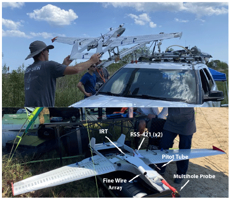
Figure 1The University of Colorado RAAVEN being prepared for launch during WiscoDISCO21 (top) and a closeup of the RAAVEN sensing systems (bottom).
For the WiscoDISCO-21 campaign, the RAAVEN was equipped with an instrument suite derived from the miniFlux payload co-developed by the National Oceanic and Atmospheric Administration (NOAA), the Cooperative Institute for Research in Environmental Sciences (CIRES), and Integrated Remote and In Situ Sensing (IRISS) at the University of Colorado. In this configuration, the aircraft was set up to measure atmospheric and surface properties to support evaluation of thermodynamic state, kinematic state, and turbulent fluxes of heat and momentum. This involves a suite of core instrumentation (see Fig. 3), including a multihole pressure probe (MHP) from Black Swift Technologies, LLC (BST); a pair of RSS421 PTH (pressure, temperature, humidity) sensors from Vaisala, Inc.; a custom finewire array, developed and manufactured at the University of Colorado Boulder; a pair of Melexis MLX90614 IR thermometers; and a VectorNav VN-300 inertial navigation system (INS). This sensor suite is logged using a custom-designed FlexLogger data logging system.
The Vaisala RSS421 sensors are identical to those used in the Vaisala RD41 dropsonde and very similar to the Vaisala RS41 radiosonde. This unit employs a linear resistive platinum temperature sensor with a resolution of 0.01 ∘C, repeatability of 0.1 ∘C, and response time (as measured within the RS41 radiosonde) of 0.5 s at 1000 hPa when moving at 6 m s−1. For relative humidity (RH), the RSS421 includes a thin-film capacitor with a resolution of 0.1 % RH and a repeatability of 2 % RH, with a temperature-dependent response time of better than 0.3 s at 20 ∘C (again, as measured within the RS41, with 6 m s−1 airflow at 1000 hPa). Finally, the pressure sensor is capacitive with a silicon diaphragm, having a resolution of 0.01 hPa and a repeatability of 0.4 hPa. For WiscoDISCO-21, a pair of these sensor modules was mounted to the top of the RAAVEN's fuselage, between the nose and the tail of the aircraft on the port side. The sensor mounting angles were offset to ensure that the two sensors would have different amounts of solar exposure as the aircraft maneuvers through the atmosphere and to allow for the detection of solar heating effects since no shading is used. Additional information on atmospheric thermodynamic state is available from an E+E EE-03 sensor that is integrated into the BST MHP and from a Sensiron SHT-85 sensor that is integrated in the custom finewire array. The EE-03 has a temperature accuracy (at 20 ∘C) of 0.3 ∘C, while the humidity accuracy is stated to be 3 % RH at 21 ∘C. The SHT-85 has a stated temperature accuracy of 0.1 ∘C (from 20–50 ∘C) and a repeatability of 0.08 ∘C, while the humidity sensor has a stated accuracy of 1.5 % RH and a repeatability of 0.15 % RH. Both the EE03 and the SHT-85 sensors have slower response times than the RSS421 sensor described above and are typically not used for scientific purposes unless there is a complete failure of the RSS421.
In addition to the SHT-85 sensor, the finewire array consists of two 5 µm diameter platinum wires extending over a 2 mm length, suspended in the free stream by supporting prongs. One wire is operated as a hotwire anemometer, with approximately 100 ∘C overheating compared to the ambient environmental temperature. The other wire is operated as a coldwire thermometer, with approximately 1 ∘C overheating relative to the surrounding environment. The wires have thermal time constants of 0.5 ms in a 15 m s−1 airflow regime and support a sampling frequency of up to 800 Hz to support measurement of turbulent fluctuations in velocity and temperature. An electronics module converts resistance change in the wires due to velocity or temperature variability to amplified voltages. For WiscoDISCO-21, the finewire was logged at 250 Hz by the FlexLogger, which is equivalent to a 7.2 cm minimum length scale at the RAAVEN's typical cruise airspeed of 18 m s−1. Time series of these recorded data are processed during post-flight analysis to transform the voltages recorded by the fine-wire module to velocity and temperature. Additionally, these measured quantities can be fit to inertial sub-range turbulence models to wavenumber spectra over suitable time intervals, producing turbulence intensity parameters epsilon (kinetic energy dissipation rate) and CT2 (temperature structure constant). The resolution (noise floor) of these parameterizations is 2.0 × 10⁻⁷ W kg−1 for epsilon and 4.5 × 10⁻⁶ K2 m for CT2. Resolution of the raw time series is 8.3 × 10⁻⁵ m s−1 for the hotwire and 1.3 × 10⁻⁴ K for the coldwire.
In addition to the EE-03 PTH measurements, the BST five-hole probe supports measurement of airspeed, angle of attack (α), and sideslip angle (β). These measurements are combined with the GPS-based ground velocities and aircraft altitude from the VectorNav VN-300 to derive the three components of the inertial wind (u, v, w), as discussed in Sect. 4. The VN-300 can be configured in a dual-Global Navigation Satellite System (GNSS) mode, under which the relative positions of two GNSS antennae are used to calculate the platform yaw. However, this setting was not used during the WiscoDISCO-21 deployment. Under dynamic conditions, the system has a stated accuracy of 0.3∘ in GPS compass heading, 0.1∘ in pitch and roll, 2.5 m horizontal position accuracy, 2.5 m vertical position accuracy when integrating information from the barometric pressure sensor, and 0.05 m s−1 accuracy in inertial velocity. Input from the system's gyroscope, accelerometer, GNSS receiver, magnetometer, and pressure sensor is filtered through an extended Kalman filter (EKF) to produce a navigation solution. VN-300 data were logged at 50 Hz resolution during WiscoDISCO-21.
Finally, RAAVEN deploys two Melexis MLX90614 IR thermometers: one looking up from the top of the aircraft and one looking down towards the surface in level flight. These sensors are factory calibrated to work in operational temperatures between −40 and 125 ∘C and to measure target brightness temperatures between −70 and 380 ∘C. They have a high accuracy (0.5 ∘C) and a measurement resolution of 0.02 ∘C. The RAAVEN-mounted MLX90614s are not stabilized to maintain a vertical orientation, meaning that the observed target is perpendicular to the reference frame of the aircraft. This requires some care when interpreting measurement from time periods when the aircraft is conducting pitch or rolling maneuvers. For WiscoDISCO-21, we leveraged the “I” version of this sensor, which has a 5∘ field of view. These sensors have a broad passband range of 5–14 µm, meaning that while it covers the infrared atmospheric window, it is also subject to radiation emitted by water vapor and other radiatively active gases. This means that there is a significant depth of atmosphere between the aircraft and a given target (e.g., cloud, surface), and atmospheric gases influence the temperature reading. Despite this range spanning the 9.6 µm O3 band, the relative proximity of the sensor to targets of interest (e.g., surface, clouds) means that this overlap is not expected to significantly influence the readings, due to the integrated path length being relatively small. Therefore, if absolute accuracy of brightness temperature is important, the sensor should be operated in close proximity to a target of interest. However, relative contributions from different surface types or atmospheric conditions can still be easily distinguished despite a lack of absolute calibration for extended distance sensing. Such gradient detection can be useful for detecting surface inhomogeneities, or for understanding whether the aircraft is operating under cloud or clear sky.
2.2 M210 UAS
The DJI M210 quadcopter was equipped with a 3-D printed top-mounted bracket for holding a 2B Technologies personal ozone monitor (POM) and an Intermet Systems iMET-XQ2 meteorology sensor (Fig. 2). The copter had a ∼ 15 min flight time with the onboard sensors without a camera. The POM measures ambient ozone using UV absorption and active humidity subtraction by measuring a whole-air sample and an ozone scrubbed sample in a 10 s duty cycle. The POM records data to its internal data storage at 10 s intervals with a log number and timestamp along with GPS coordinates and instrumentation metrics (optical cell pressure and temperature). The iMET system records temperature, humidity, and pressure along with GPS coordinates and a timestamp to internal data storage. Each instrument (the POM and iMET) had individual data logging systems and separate power supplies. Both the POM and the iMET had GPS capabilities with the POM logging inconsistently and the iMET logging GPS more consistently. Each instrument and the UAS flight recorder logged timestamps. The iMET recorded observations of temperature, relative humidity, humidity temperature, and pressure at a frequency of 10 Hz. The POM recorded ozone observations at a frequency of 0.1 Hz. The POM, iMET, and M210 timestamps drifted up to 60 s from the other logged data. The flight log recorded the M210 positioning (altitude, latitude, longitude) at 100 Hz. The M210 flight logs, iMET data, and POM data were each downloaded separately after each series of flights.
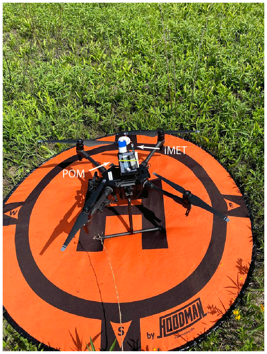
Figure 2DJI M210 multirotor UAS with bracket-mounted POM and iMET.
2.3 Chiwaukee lidar system
A Halo Photonics Stream Line XR Doppler lidar (Pearson et al., 2009) was deployed on the roof of the Chiwaukee Prairie air monitoring station (Fig. 3), approximately 3 m a.g.l. This is the same system that is regularly deployed as part of the Space Science and Engineering Center (SSEC) Portable Atmospheric Research Center, SPARC (Wagner et al., 2019). The Doppler lidar actively emits pulses of near-infrared radiation at a wavelength of 1.5 µm. This wavelength is long enough that molecular scattering causes little attenuation of the signal, but it is short enough that it is sensitive to aerosols that are suspended within the planetary boundary layer.
The Doppler lidar uses velocity-azimuth display (VAD) scans of the Doppler lidar to retrieve profiles of wind speed and direction. In VAD, an instrument capable of measuring along-beam velocity (like a Doppler radar or lidar) stares at multiple azimuths at a non-zenith elevation angle over a short period of time and then reconstructs the profile of winds above the lidar by assessing how the along-beam velocity changes as a function of azimuth and range. For WiscoDISCO-21, the VAD scans were configured with six azimuthal stares per profile (at azimuths of 0, 60, 120∘, and so on) with an elevation angle of 70∘. Range gates were 18 m. VAD scans were conducted every 4 min, and each VAD took approximately 45 s to complete. Between VADs, the lidar reverted to vertical stares in order to capture profiles of backscatter and vertical velocity. Since the lidar depends on the presence of scatterers to have a detectable signal return, the depth of the retrieved wind profiles varied significantly throughout the experiment from as shallow as 200 m to as deep as 2 km.
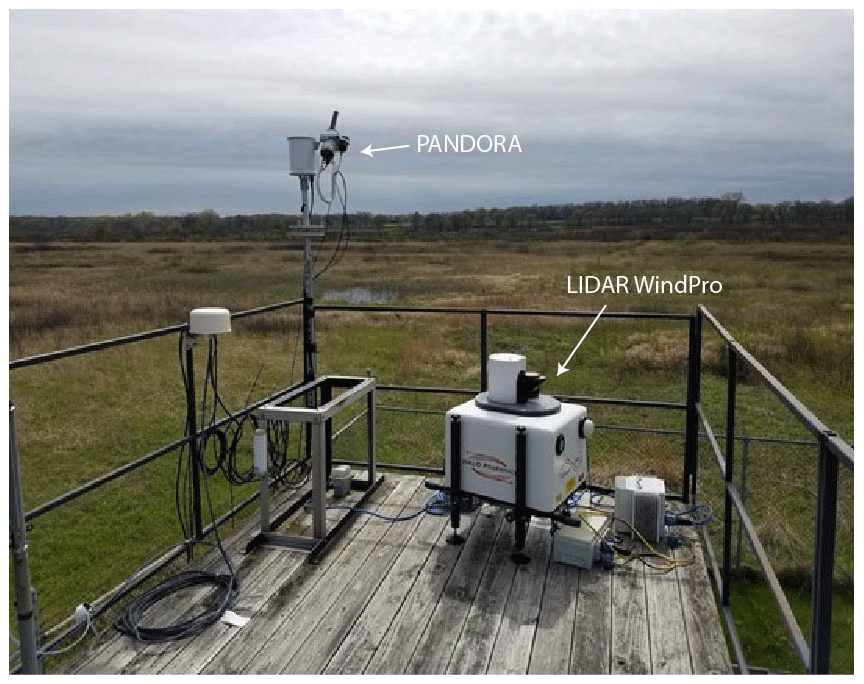
Figure 3Roof of the Chiwaukee Prairie air monitoring system, showing the PANDORA (upper left) and Doppler lidar (right center). The wooden floor pictured here is approximately 3 m a.g.l.
The Chiwaukee Prairie State Natural Area is a 1.97 million square meters shoreline prairie managed by the Wisconsin Department of Natural Resources (WiDNR) located along the shoreline of Lake Michigan and adjacent to the Wisconsin–Illinois border. The WiDNR operates an air monitoring station (Airs ID 55-059-0019) for Kenosha County within this area, located at 11838 First Court in Pleasant Prairie, WI. This location was chosen due to its suitability for UAS flight operations and the regular influence of lake breeze circulations at the site. As a result of these lake breezes, the WiDNR's Chiwaukee Prairie Monitor regularly observes some of the highest ozone concentrations in the state (Stanier et al., 2021) with a 2015–2017 design value of 78 ppb (Cleary et al., 2022), where the federal ozone standard is 70 ppb for an 8 h average. Land use in the region is mixed suburban housing and farming, with two marinas directly south of the research site. Chiwaukee Prairie has trail access along Al Kemper Trail and 122nd Street that is isolated from automobile, bicycle, and most pedestrian traffic. The M210 flights were conducted near the WiDNR Air Monitoring site (latitude: 42.5045, longitude: −87.8095), and the RAAVEN flight operations were conducted on Al Kemper Trail or 122nd St. to provide ample room for take-off and landing (Fig. 4).
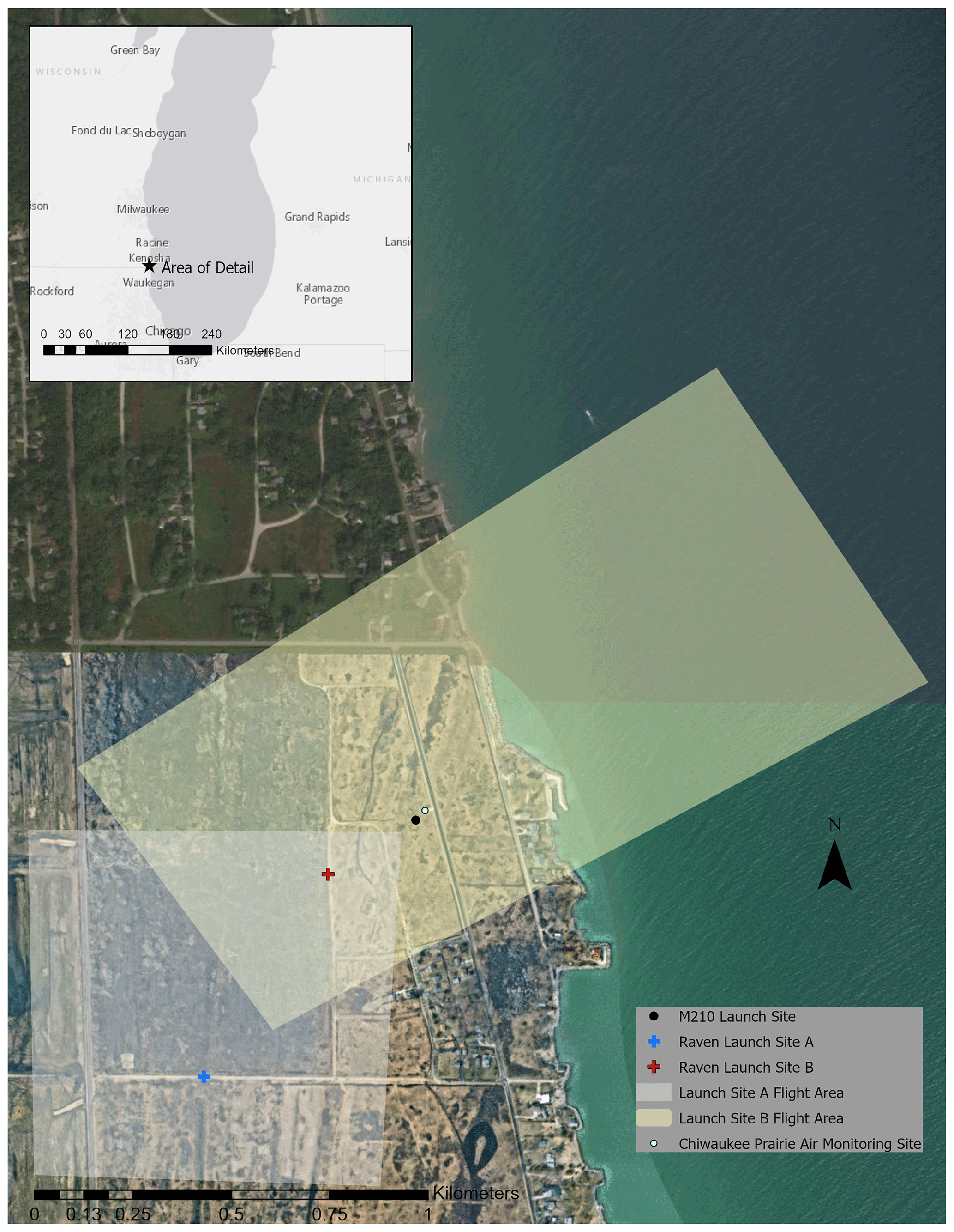
Figure 4Research site map including Chiwaukee Prairie air monitor and locations for launch sites for M210 and RAAVEN. Map created using Esri ArcPro version 2.52 using ArcPro basemap imagery.
The primary goal for the field campaign was to capture elevated ozone concentration events resulting from lake breeze circulations at the site. The deployment strategy for selecting a time window for field operations was dictated by ozone and meteorological forecasts that predicted light southerly winds for an extended period that would both (a) increase the likelihood of onshore lake breeze flow from weaker southerly winds and (b) drive pollutant transport from the Chicago metro area to the site.
Forecasts from both the WiDNR and Realtime Air Quality Modeling System (RAQMS) were used to select an ideal deployment period. The dates of 21–26 May 2021 were chosen as meeting those requirements. The selection of the time period for the campaign was dictated by capturing a combination of lake breeze and ozone events. An acceptable window for operations from late 23 May through mid-June was targeted because of the higher frequency of high-ozone and lake breeze events occurring in this region during late spring/ early summer (see Cleary et al., 2022, Supplement, for a list of high ozone events for the years 2013–2019 at Chiwaukee Prairie). Once the operations window was approaching, the team used the RAQMS forecast model (Fig. 5) and consulted with the Wisconsin Department of Natural Resources (WiDNR) Air Quality Division's meteorologist to decide on a “go time” to initiate deployment from all collaboration partners for an 8 d campaign. The go time required evidence that synoptic flow would have a southerly component for a few days (normally brought about by a high-pressure system over the Ohio River valley) with limited precipitation events. Flights were canceled during days in which high ozone and southerly-southeasterly lake breeze were not expected (Table 1).
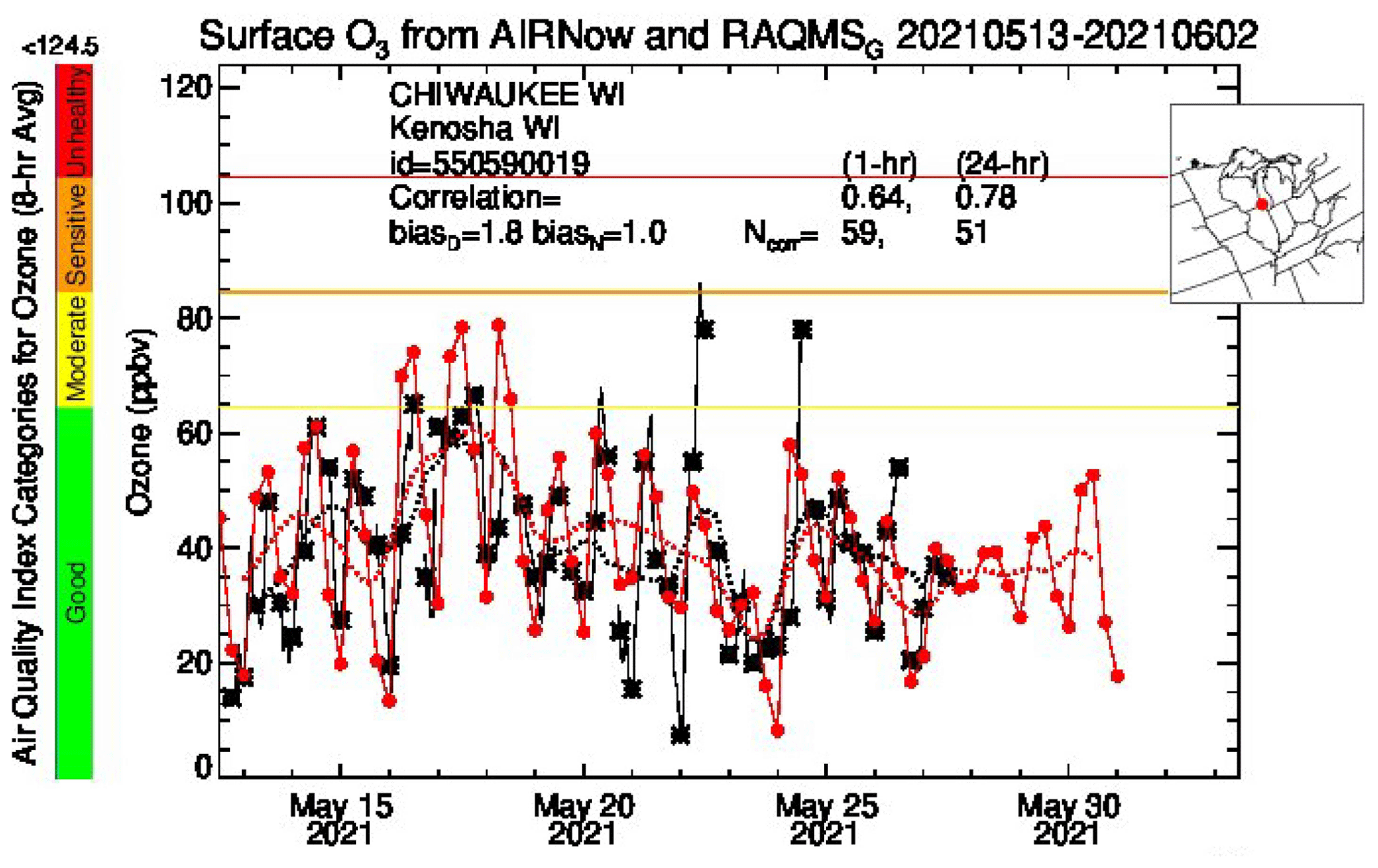
Figure 5The 8 h ozone concentrations from RAQMS forecast (red) and observations (black) for 13–26 May 2021 at Chiwaukee Prairie.
Table 1UAS flight days and conditions for the WiscoDISCO-21 field campaign. Flight patterns A and B are depicted in Fig. 6a.
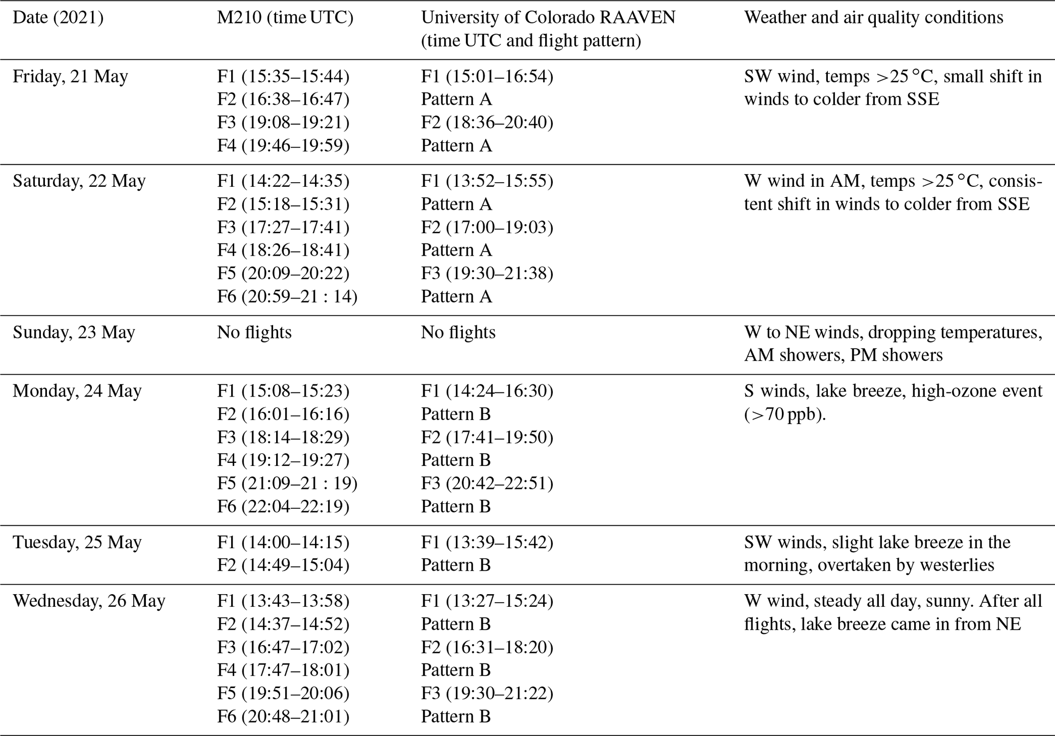
Flights were conducted in the time window 08:00–17:00 local time, CDT (13:00–22:00 UTC) (Table 1). The RAAVEN platform features 2 h flight times and was deployed to complete up to three flights per day. The M210 flew slow ascents to 120 m a.g.l. with an approximate 15 min flight time, completing up to six flights per day, and the sampling pattern was designated to achieve maximum overlap with the RAAVEN flight times by conducting two flights per RAAVEN flight.
During WiscoDISCO-21, the RAAVEN completed 12 flights, totaling 25.4 flight hours, operating under a Certificate of Authorization (COA) from the US Federal Aviation Administration (FAA) to allow flights up to 518 m a.g.l. Figure 6a shows a map of the RAAVEN flights, while Fig. 2b includes a histogram of the altitudes covered by these flights. Flights were designed to follow two distinct flight patterns: A and B to capture over-prairie profiles using a circular pattern with holding at altitudes 400, 250, 150, 100, and 50 m a.g.l. and over-water/over-prairie profiles using an extended racetrack pattern that traversed the shoreline, with holding altitudes at 400, 250, 150, 100, and 50 m a.g.l. (see Fig. 6c for the two flight patterns). Figure 7 shows histograms of the measurements obtained by the RAAVEN over the length of the campaign, including temperature, relative humidity, wind speed, wind direction, air pressure, and surface and sky brightness temperature.
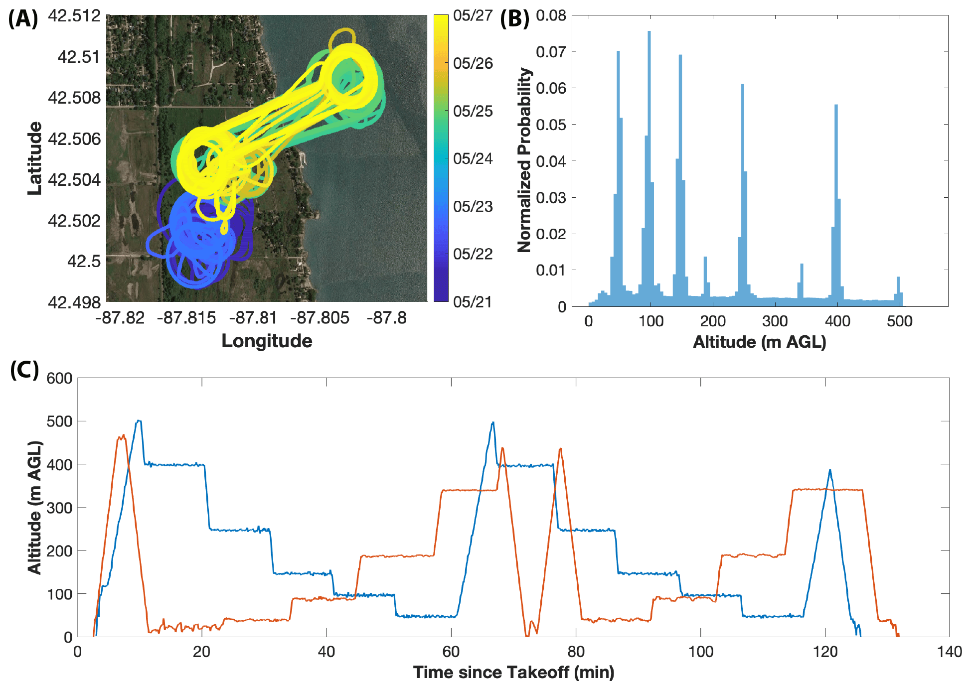
Figure 6A map showing the flight tracks for the RAAVEN with blue showing flight pattern A and yellow or green showing flight pattern B (a), a histogram of altitudes sampled by the RAAVEN (b), and example time–height plots of the two types of RAAVEN flights (c). The “normalized probability” presented for a given bin is the number of elements in a given bin divided by the total number of elements in the input data, so that the integral of the histogram equals 1. Background maps are © Google Maps 2021, downloaded through their API.
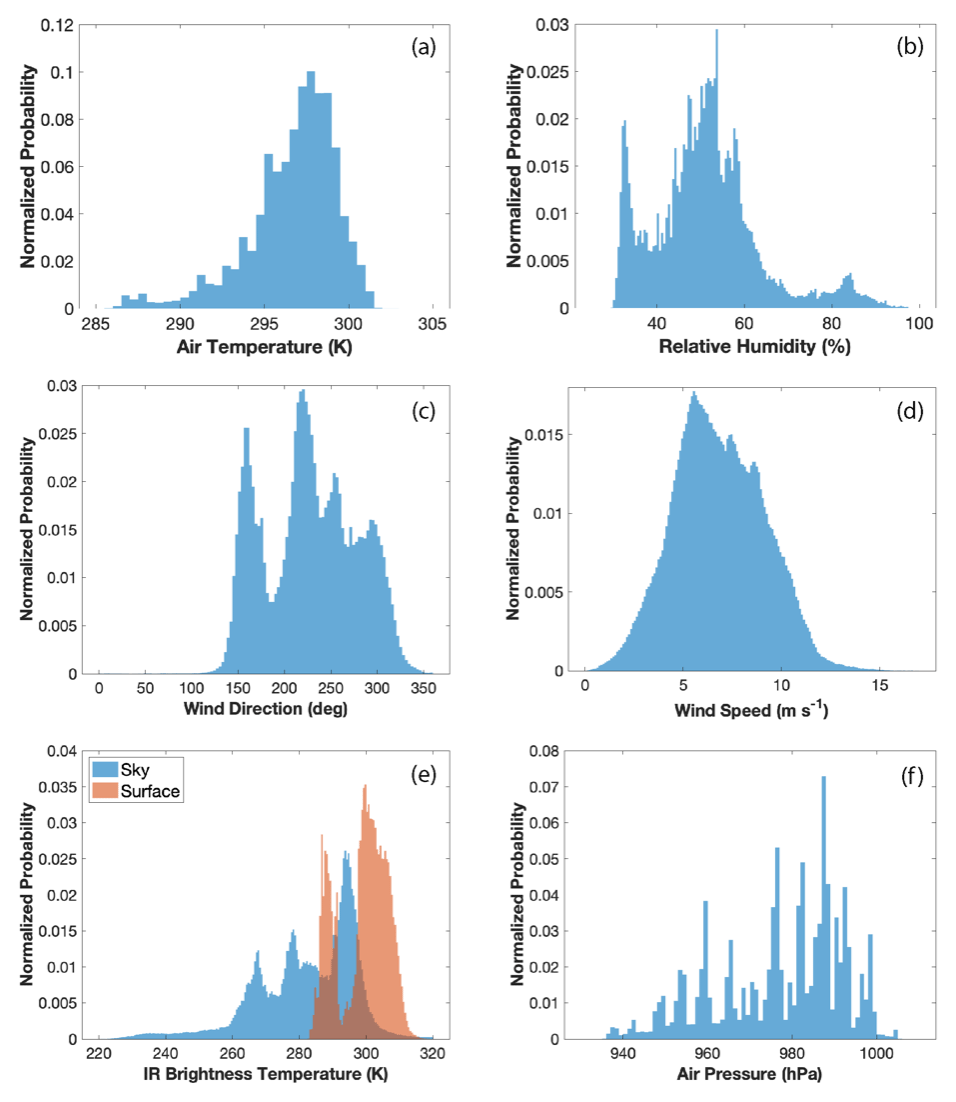
Figure 7Histograms of (a–f) temperature, relative humidity, wind direction, wind speed, IR brightness temperatures, and air pressure, as measured by the RAAVEN during WiscoDISCO-21. As in Fig. 6, the “normalized probability” presented for a given bin is the number of elements in a given bin divided by the total number of elements in the input data, so that the integral of the histogram equals 1.
4.1 University of Colorado RAAVEN UAS
Data collected by the different sensors carried by the RAAVEN during WiscoDISCO-21 were logged at a variety of different logging rates. The finewire system was logged at 250 Hz, the fastest rate of all of the sensors. The BST MHP was logged at 100 Hz and the VectorNav VN-300 at 50 Hz, the Melexis IR sensors and variables related to finewire status were logged at 20 Hz, while data collected from the PixHawk autopilot and Vaisala RSS421 sensors were logged at 5 Hz. Each logging event carried out by the FlexLogger includes a sample time from the logger CPU clock, allowing for post-collection time alignment between the different sensors. These sample times, along with artificial 5, 20, 50, 100, and 250 Hz clocks spanning the sample times between initial GPS lock and the last recorded sample time for the VN-300, are used to align the different variables to a set of common clocks, primarily through one-dimensional linear interpolation. One exception to the linear interpolation is the yaw estimate, which is circular in nature (ranging between −180 and 180∘) and therefore uses a “nearest” interpolation to ensure that the transition from 360 to 0∘ is not represented as 180. During this interpolation process, a limited number of points sharing a common sample time with another point are removed from the record. Once these time variables are established, a base_time variable is established using the 250 Hz timestamp and offsets from base_time are then calculated for all different logging resolutions.
The resampled (in time) dataset includes a variety of derived and measured quantities. Aircraft positions, including latitude, longitude, and altitude, are measured by the VN-300. The aircraft altitude is corrected using a combination of various inputs from onboard GPS and pressure altimeters, as neither of these altitude estimates can be used reliably as a definite flight altitude. Pressure altitude is subject to drift over the duration of a single flight due to atmospheric evolution over a 2.5 h window, potentially resulting in values at landing that are higher or lower than those at take-off. Similarly, the accuracy of the GPS altitude is insufficient to capture the vertical position of the aircraft to the level of detail required. To calculate a true altitude, a combination of the autopilot altitude, VN-300 altitude, and VN-300 pressure is used. First, a flight_flag variable is computed using airspeed and altitude information from the autopilot. Any data points with airspeed exceeding 10 m s−1 and an altitude exceeding 5 m a.g.l. is flagged as a time when the aircraft is flying (flight_flag = 1). The point at 200 samples (4 s) prior to the first point in the record where the aircraft is deemed to be flying is recorded as the initial take-off index, while the data point at 200 samples (4 s) after the last point in the record where the aircraft is deemed to be flying is recorded as the landing index. The difference between the autopilot altitude at these two indices is added into the flight record on a time step-by-time step basis, to correct for temporal drift in pressure. A linear fit is then calculated to relate the VN-300 pressure and the difference between the VN-300-reported altitude and the autopilot-reported altitude. This pressure-dependent altitude correction is then applied to the VN-300-reported altitude to derive a final altitude.
Wind estimation from fixed-wing aircraft requires the combination of several different measurements related to airspeed, aircraft motion, and airflow over the aircraft (see van den Kroonenberg et al., 2008). These measurements need to be of sufficient quality, and angular offsets and logging delays need to be considered and removed. For RAAVEN, true airspeed (TAS) biases have a large impact on derivation of wind speed, while the angular offsets between the MHP and INS and time lag between the GPS and in situ measurements have smaller impacts. These potential sources of error are corrected for using an optimization technique, where small adjustments are made to the individual parameters, and the combination that results in the wind solution with the smallest overall variance is selected as the correct winds.
For the RAAVEN WiscoDISCO-21 dataset, TAS is calculated using measurements from the MHP and RSS421 probe using Eq. (1) from Brown et al. (1983):
where ρ is the density of air calculated using the static pressure reported from the MHP, temperature from the RSS421, and the specific gas constant for dry air. is defined as
where sin 2θa is the total aerodynamic angle of the MHP, calculated using the angle of attack (α) and sideslip angle (β) reported by the MHP.
Based on testing in a temperature chamber, the pressure sensors used in this version of the MHP were found to have non-linear temperature dependencies. This requires the application of an additional temperature-dependent correction to ensure that an artificial alteration of TAS with altitude was not present. Additional information on the calculation of airspeed and other quantities from the MHP can be found in de Boer et al. (2022a).
Derivation of the RAAVEN's thermodynamic measurements included multiple processing steps. First, data from the two RSS421 sensors are averaged to attempt to reduce the influence of any solar exposure of the sensors. Previous evaluations of the potential for solar contamination have not revealed any specific biases on the observation (see de Boer et al., 2022a). Over the course of the WiscoDISCO-21 campaign, the two sensors varied by less than 0.5 ∘C (Fig. 8). The averaged temperature time series was then used to calibrate the coldwire data by applying a linear fit to the relationship between the coldwire voltage and the temperature measured by the RSS421 sensor. The RSS421 relative humidity values were also averaged. Typically, the RH measurements agreed to within 2 %.
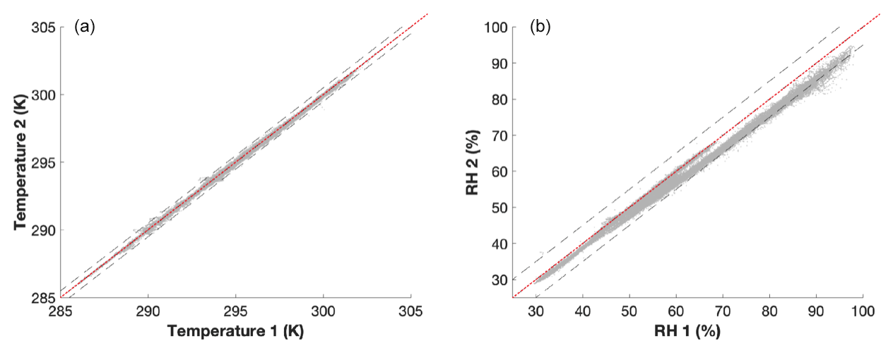
Figure 8A comparison of temperature (a) and relative humidity (b) observations from the two Vaisala RSS-421 sensors on RAAVEN for all flights. The red dotted lines represent a one-to-one agreement, with the dashed black lines representing 0.5∘ (for temperature) and 5 % (for relative humidity) deviation from perfect agreement.
All quantities measured by the RAAVEN have data quality flags associated with them. For the RSS421-derived temperature, the flag is set to zero for good data and set to 1 for times when any of the following occur: (a) the absolute value of the difference between the temperature from either individual sensor and the output temperature is greater than 0.5 ∘C, (b) the absolute value of the difference between the output temperature and the temperature from the EE-03 sensor on the MHP exceeds 5 ∘C, (c) the recorded error flag of either RSS421 sensor is active, or (d) the aircraft is not flying. For the RH measurement from the RSS421, a similar set of criteria are used to activate the data quality flag, except the limits are set to be 6 % between RSS421 sensors and 15 % between the output RH value and the MHP-provided RH value. The relative humidity values from the MHP are significantly impacted by the exposure of that sensor to sunlight and the associated impact on sensor temperature. This is not corrected for, resulting in large fluctuations in the RH values at times. As a result, this measurement (from the MHP) only provides a reality check to ensure that the RSS421 sensors are reporting accurate values, and therefore such a large offset (15 %) is allowed. The more important comparison is between the two RSS421 sensors, which should agree much more closely, as they are the same sensor type and are mounted within close proximity of one another. The coldwire temperature data quality flag is activated when the difference between the coldwire temperature and either of the RSS421 temperatures exceeds 1 ∘C, when the absolute value of the difference between the coldwire temperature and the MHP temperature exceeds 3 ∘C, when the coldwire voltage is observed to fall outside of the 0–4 V analog range, or when the aircraft is not flying. Finally, the pressure quality control flag for the pressure measurement from the VN-300 is activated if the absolute value of the difference between the reported VN-300 static pressure and that measured by either of the RSS421 sensors exceeds 2.5 hPa. The RSS421 pressure measurements are not used because they are believed to be biased low due to the airflow passing over their location on the aircraft.
In addition to the flags discussed above, we include a three-stage flag for the wind measurements, which is set to 0 (good data), 1 (suspect data), or 2 (bad data). Data are determined to be bad if any of the following conditions were met.
-
The measured angle of attack or sideslip exceeds 20∘, with values between 10–20∘ flagged as “suspect”.
-
The true airspeed (TAS) is below 10 m s−1.
-
Any of the MHP ports are deemed to be blocked, as determined by the differential pressure value for any of the sensors falling below −100 Pa.
-
The moving window variance of the MHP-derived TAS over 40 s is less than 5.
-
The aircraft is not flying.
-
The difference between the MHP TAS and that from the Pitot probe is greater than 5 m s−1.
Finally, we included two additional flags in the data stream to allow data users to better understand aircraft flight state and support sampling during specific phases of flight. These flags include the “Flight_Flag” introduced previously, as well as a “Flight_State” flag. The Flight_State flag includes information on whether the craft is flying straight (0) or is turning (1) in the ones place, whether the aircraft is descending (0), level (1), or ascending (2) in the tens place, and whether the aircraft is in flight (1) or not (0) in the hundreds place. If, for example, a data user wanted to analyze straight, level flight legs, they would search for data with Flight_State equal to 110. These flags are derived from information from a combination of sensors, including the altitude variable described above, the aircraft yaw, and the Flight_Flag variable described earlier on in this paragraph.
The accuracy of the RAAVEN observations has been evaluated in previous studies. For example, a comparison of RAAVEN data with measurements collected by radiosondes launched from the Barbados Cloud Observatory was conducted in recent work from de Boer et al. (2022b). While radiosondes in that evaluation were launched approximately 20 km to the southeast, the air sampled by both systems was largely representative of the marine boundary layer, implying limited spatial variability. In that evaluation, the observations from the RAAVEN were very well correlated with those from the radiosondes and do not show any positive or negative bias, supporting the idea that the RAAVEN measurements provide an accurate depiction of the lower atmosphere. In addition, recent work allowed for direct comparison of RAAVEN data to observations collected by radiosondes and a 60 m tower at the US Department of Energy's Southern Great Plains (SGP) research site. That study, de Boer et al. (2022a), similarly provided confidence in the RAAVEN observations, showing close statistical agreement between the different data sources.
4.2 M210 UAS
Data from the M210 flight controller, the POM, and the iMET were all logged to individual instrument internal data storage with independent timestamps. The average flight time of the M210 was 13.96 min. The POM instrument logged data at 0.1 Hz. The iMET logged data every 10 Hz, and the M210 flight log recorded UAS GPS positioning and flight statistics at 100 Hz. The ozone concentrations from the POM are adjusted to calibrated values, where ozone calibrations were conducted before every set of two flights for the M210 using a 2BTech model 306 ozone calibration source (Fig. 9). Data quality flags are established as 0 being no concern, 1 being time flag, and 2 being calibration and time flag. The time flag indicates flights where the time offset between the M210 and the instrument time offset is large (iMET >10 s or POM >30 s). The calibration flag indicates when the POM was not responsive to the ozone calibration source (Flight 5 on 24 May) after an over-water flight. All times were averaged to 90 s and compressed to the time window of observations for a single M210 ascent using the M210 timestamp. A timestamp for 90 s averaged data from all instrumentation on the M210 was generated by using the M210 timestamp as primary and adjusting to a time offset in either the POM or the iMET for the start of a flight; then each variable was averaged for every 90 s interval of the flight. A 1σ standard deviation is presented as the uncertainty for the 90 s averages. The iMET observations of temperature, relative humidity, pressure, and humidity temperature are presented using the 90 s averages with uncertainty as 1σ standard deviations. Each flight ascent start and end were determined by observed changes in atmospheric pressure by the iMET sensor, altitude change in the M210, or noted time of ascent in field notebook for the POM. The altitudes for each observation were obtained by averaging the M210 flight log altitude data for the 90 s timestamps. The flight data timestamps varied slightly for each data source. The POM time drift was the most pronounced, with an average difference between the iMet of ∼ 24 s. The POM's time was adjusted manually throughout the campaign as the time would drift over the course of one flight. The average difference between the iMet and the M210 over 20 flights was ∼ 4 s. Only 20 % of flights had a time difference between iMET and M210 greater than 10 s. Instrument battery loss occurred for the iMET system, which resulted in lost data for two flights on 26 May 2021.

Figure 9A sample POM calibration from 24 May 2021. The linear regression fit gives y=0.9689 (±0.0061) x+0.83 (±0.35), R2=0.9937. Each calibration concentration had a 5 min duration with the POM logging 10 s data.
Intercomparison between observations made via instrumentation on the M210 at 5 m a.g.l. and at the Wisconsin DNR ground station show a linear agreement between the observations (Fig. 10). The linear agreement is better for the iMET temperature and the ground station temperature with R2=0.970 in comparison to R2=0.955 for O3 observations. The O3 linear fit, O3 (POM)=0.944 (±0.044) O3 (DNR)−3.3 (±1.9), has a negative intercept. The uncertainties in the POM's O3 concentrations are much larger than uncertainties in the ground station instrumentation. The linear agreement between the different instrumentation on separate observation platforms demonstrates that the M210 platform instrumentation provides an accurate, albeit less precise, representation of the atmosphere.
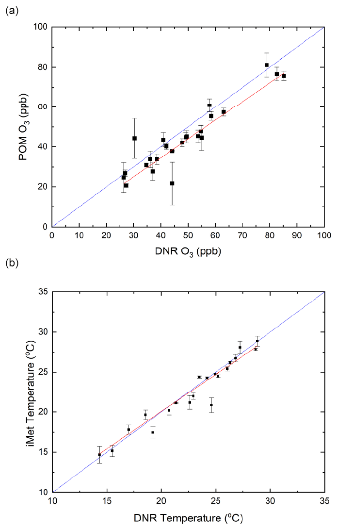
Figure 10Intercomparison between measurements from instrumentation on the M210 at 5 m a.g.l. and at the Wisconsin DNR ground station for (a) O3 (ppb) observations and (b) temperature (∘C). Blue lines depict 1:1 agreement, and red lines depict the linear regression best fit with (a) O3 (POM)=0.944 (±0.044) O3 (DNR)−3.3 (±1.9), R2=0.955 and (b) TiMET=0.929 (±0.038) TDNR+1.48 (±0.93), R2=0.970.
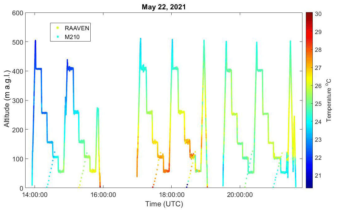
Figure 11Temperatures (∘C) measured from University of Colorado RAAVEN (◦) and the M120 (□) on 22 May 2021. RAAVEN was flying over-prairie circular spirals in pattern A.
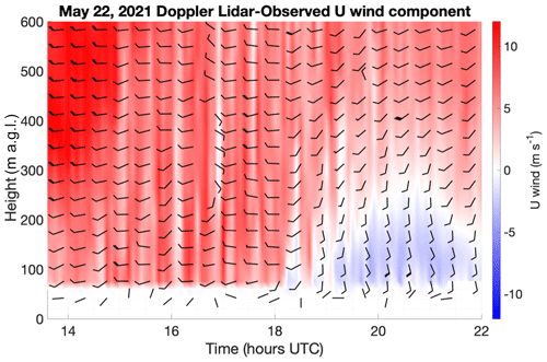
Figure 12Time–height cross section of the u (zonal) component of the Doppler-lidar-observed horizontal winds (in m s−1), overlaid with horizontal wind barbs (in knots) plotted according to the standard convention from 22 May 2021. Wind barbs are thinned by a factor of 5 in the time dimension and a factor of 2 in the height dimension to aid readability.
A community data repository has been established for this field campaign at https://zenodo.org/communities/wiscodisco21/ (last access: 21 April 2022). The datasets in the repository cover the merged iMET and POM datasets from the M210 (DOI: https://doi.org/10.5281/zenodo.5160346, Cleary et al., 2021a) as .txt files, the RAAVEN dataset (DOI: https://doi.org/10.5281/zenodo.5142491, de Boer et al., 2021) as .cdf files, and the Doppler lidar wind profiler (DOI: https://doi.org/10.5281/zenodo.5213039, Cleary et al., 2021b) as .cdf files. M210 files have a naming convention that includes WiscoDisco_M210_YYYYMMDD_F#, where the flight number for the day is indicated by F#. RAAVEN files have a naming convention that includes WiscoDisco_CU-RAAVEN_YYYYMMDD_hhmmss_B1.nc, where YYYYMMDD is the year, month, and day that the data were collected; hhmmss is the time of power on for the aircraft; and B1 is the data processing level, where B1 files have had data quality checks and post-processing (e.g., coldwire calibration and wind estimation) applied. The Doppler lidar files have a naming convention that includes chiwaukee_wind_profiles_YYYYMMDD and chiwaukee_stare_YYYYMMDD. All datasets include geospatial information (latitude, longitude, altitude) and timestamps in UTC.
The WiscoDISCO-21 project demonstrates how UASs can be used to sample a complex circulation near the surface without causing major disruption to people, wildlife, and ecosystems in the area. An example of a characterization of lake breeze incursion is shown in Figs. 11 and 12, which include the temperature profiles from the M210 and RAAVEN (Fig. 11) and Doppler lidar u wind component (Fig. 12). The temperature profiles from the M210 and RAAVEN show a notable temperature inversion in the late afternoon below 150 m, and the Doppler lidar u wind component shows easterly winds arriving after 18:00 UTC. The combination of u component winds from Doppler lidar and the temperature observations from the UAS platforms is consistent in demonstrating a marine layer incursion with maximum height of approximately 250 m a.g.l. at 21:00 UTC collapsing to a height of 100 m a.g.l. by 22:00 UTC. The nonuniform start to the lake breeze onset fluctuated, shown as shifting u component winds from easterly to westerly after 18:00 UTC (Fig. 12) and disagreement with the lowest-altitude observations from the M210 and RAAVEN between 18:30–19:00 UTC (Fig. 11). The distance between the M210 launch site and the RAAVEN landing site complicates the low-altitude observations of temperatures between 18:00 and 19:00 UTC, which may also indicate the very limited incursion of the lake breeze at that time.
The 2021 WiscoDISCO field campaign incorporated the use of two UAS platforms for meteorological and chemical measurements in the atmosphere, a multirotor completing vertical profiles up to 120 m a.g.l. and a fixed wing executing flight patterns up to 500 m a.g.l. alongside a lidar WindPro instrument capable of sensing winds and aerosol backscatter from altitudes of 100–2000 m a.g.l. The overlapping domains are useful for characterizing low-altitude mesoscale meteorology of the lake breeze at a shoreline environment that regularly observes ozone enhancement events during onshore flow. Data from all instruments and platforms have been compiled, quality-control tested, and uploaded to a community repository. The collaborative field campaign involved teams from four different universities and obtained continuous lidar data in conjunction with 24 flight hours of fixed wing and 6 flight hours of multi-rotor vertical profiles on days likely impacted by lake breeze.
The data from the WiscoDISCO-21 campaign can be used to evaluate the markers for lake breeze incursion overland in winds, temperatures, chemical composition, and optical properties (backscatter). The thermodynamic conditions for lake breeze incursion at a local scale can be determined through the evaluation of horizontal and vertical winds, atmospheric stability, and potential temperature. The positioning of pollutants with respect to the marine layer markers can also be investigated.
PAC is the PI of this project and was responsible for data collection, overseeing data analysis from the M210, field campaign planning and logistics, and the writing and editing of this document. BK was responsible for data collection for the M210 in the field; JT was responsible for data analysis, quality control, and data formatting for the repository for the M210; and AV was responsible for data analysis for the M210. JPH was responsible for piloting the M210 and the writing and editing of this paper. GdB was responsible for coordination and execution of the University of Colorado RAAVEN flights and for development, writing, and editing of the publication. SB and JH contributed to the collection of the RAAVEN dataset as field operators and supported the development of this paper. DL supplied instrumentation for the RAAVEN UAS and contributed to the writing of the paper. TW and RBP were responsible for data collection, data analysis of the Doppler lidar instrumentation, and writing and editing this document, and RBP assisted in field planning.
Gijs de Boer works as a consultant for Black Swift Technologies, who manufacture the multi-hole pressure probe used in the collection of the RAAVEN dataset.
Any opinions, findings, and conclusions or recommendations
expressed in this material are those of the author(s) and do not necessarily
reflect the views of the National Science Foundation.
Publisher’s note: Copernicus Publications remains neutral with regard to jurisdictional claims in published maps and institutional affiliations.
The UW–Eau Claire team acknowledges support from the Student Blugold Commitment Differential Tuition program. The University of Colorado team acknowledges financial support from the University of Wisconsin–Eau Claire through a sub-contract supported by the US National Science Foundation, as well as support from the NOAA Physical Sciences Laboratory. The authors thank Nathan Taminger and Paul McKinley for their participation in the WiscoDISCO-21 field campaign.
This research has been supported by the National Science Foundation (grant no. 1918850).
This paper was edited by Bo Zheng and reviewed by two anonymous referees.
Abdi-Oskouei, M., Carmichael, G., Christiansen, M., Ferrada, G., Roozitalab, B., Sobhani, N., Wade, K., Czarnetzki, A., Pierce, R. B., Wagner, T., and Stanier, C.: Sensitivity of Meteorological Skill to Selection of WRF-Chem Physical Parameterizations and Impact on Ozone Prediction During the Lake Michigan Ozone Study (LMOS), J. Geophys. Res.-Atmos., 125, e2019JD031971, https://doi.org/10.1029/2019jd031971, 2020.
Brown, E. N., Friehe, C. A., and Lenschow, D. H.: The use of pressure-fluctuations on the nose of an aircraft for measuring air motion, J. Clim. Appl. Meteorol., 22, 171–180, https://doi.org/10.1175/1520-0450(1983)022<0171:Tuopfo>2.0.Co;2, 1983.
Caicedo, V., Delgado, R., Luke, W. T., Ren, X. R., Kelley, P., Stratton, P. R., Dickerson, R. R., Berkoff, T. A., and Gronoff, G.: Observations of bay-breeze and ozone events over a marine site during the OWLETS-2 campaign, Atmos. Environ., 263, 118669, https://doi.org/10.1016/j.atmosenv.2021.118669, 2021.
Cleary, P., Hupy, J., Kies, B., Tirado, J., and Voon, A.: UWEC and Purdue M210 Data for WiscoDISCO21 (Version V2), Zenodo [data set], https://doi.org/10.5281/zenodo.5160346, 2021a.
Cleary, P., Wagner, T. J., and Pierce, R. B.: UW-Madison SSEC Lidar Wind Profiler for WiscoDISCO 21 (Version V1), Zenodo [data set], https://doi.org/10.5281/zenodo.5213039, 2021b.
Cleary, P. A., Fuhrman, N., Schulz, L., Schafer, J., Fillingham, J., Bootsma, H., McQueen, J., Tang, Y., Langel, T., McKeen, S., Williams, E. J., and Brown, S. S.: Ozone distributions over southern Lake Michigan: comparisons between ferry-based observations, shoreline-based DOAS observations and model forecasts, Atmos. Chem. Phys., 15, 5109–5122, https://doi.org/10.5194/acp-15-5109-2015, 2015.
Cleary, P. A., Dickens, A. J., McIlquham, M., Sanchez, M., Geib, K., Hedberg, C., Hupy, J., Watson, M. W., Fuoco, M., Olson, E. R., Pierce, R. B., Stanier, C., Long, R., Valin, L., Conley, S., and Smith, M.: Impacts of lake breeze meteorology on ozone gradient observations along Lake Michigan shorelines in Wisconsin, Atmos. Environ., 269, 118834, https://doi.org/10.1016/j.atmosenv.2021.118834, 2022.
de Boer, G., Borenstein, S., Hamilton, J., Rhodes, M., Choate, C., and Cleary, P.: CU RAAVEN data for WiscoDISCO21, Zenodo [data set], https://doi.org/10.5281/zenodo.5142491, 2021.
de Boer, G., Borenstein, S., Calmer, R., Cox, C., Rhodes, M., Choate, C., Hamilton, J., Osborn, J., Lawrence, D., Argrow, B., and Intrieri, J.: Measurements from the University of Colorado RAAVEN Uncrewed Aircraft System during ATOMIC, Earth Syst. Sci. Data, 14, 19–31, https://doi.org/10.5194/essd-14-19-2022, 2022a.
de Boer, G., Elston, J., Houston, A., Pillar-Little, E., Argrow, B., Bell, T., Chilson, P., Choate, C., Greene, B., Islam, A., Detweiler, C., Jacob, J., Natalie, V., Rhodes, M., Rico, D., Stachura, M., Lappin, F., Whyte, S., and Wilson, M.: Evaluation and Intercomparison of Small Uncrewed Aircraft Systems Used for Atmospheric Research, Journal of Atmospheric and Oceanic Technology, in preparation, 2022b.
Doak, A. G., Christiansen, M. B., Alwe, H. D., Bertram, T. H., Carmichael, G., Cleary, P., Czarnetzki, A. C., Dickens, A. F., Janssen, M., Kenski, D., Millet, D. B., Novak, G. A., Pierce, B. R., Stone, E. A., Long, R. W., Vermeuel, M. P., Wagner, T. J., Valin, L., and Stanier, C. O.: Characterization of ground-based atmospheric pollution and meteorology sampling stations during the Lake Michigan Ozone Study 2017, J. Air Waste Manage., 71, 866–889, https://doi.org/10.1080/10962247.2021.1900000, 2021.
Dye, T. S., Roberts, P. T., and Korc, M. E.: Observations of transport processes for ozone and ozone precursors during the 1991 Lake Michigan Ozone Study, J. Appl. Meteorol., 34, 1877–1889, https://doi.org/10.1175/1520-0450(1995)034<1877:ootpfo>2.0.co;2, 1995.
Elston, J., Argrow, B., Stachura, M., Weibel, D., Lawrence, D., and Pope, D.: Overview of Small Fixed-Wing Unmanned Aircraft for Meteorological Sampling, J. Atmos. Ocean. Tech., 32, 97–115, https://doi.org/10.1175/jtech-d-13-00236.1, 2015.
Foley, T., Betterton, E. A., Jacko, P. E. R., and Hillery, J.: Lake Michigan air quality: The 1994-2003 LADCO Aircraft Project (LAP), Atmos. Environ., 45, 3192–3202, https://doi.org/10.1016/j.atmosenv.2011.02.033, 2011.
Frew, E. W., Argrow, B., Borenstein, S., Swenson, S., Hirst, C. A., Havenga, H., and Houston, A.: Field observation of tornadic supercells by multiple autonomous fixed-wing unmanned aircraft, J. Field Robot., 37, 1077–1093, https://doi.org/10.1002/rob.21947, 2020.
Geddes, J. A., Wang, B., and Li, D.: Ozone and Nitrogen Dioxide Pollution in a Coastal Urban Environment: The Role of Sea Breezes, and Implications of Their Representation for Remote Sensing of Local Air Quality, J. Geophys. Res.-Atmos., 126, e2021JD035314, https://doi.org/10.1029/2021jd035314, 2021.
Gronoff, G., Robinson, J., Berkoff, T., Swap, R., Farris, B., Schroeder, J., Halliday, H. S., Knepp, T., Spinei, E., Carrion, W., Adcock, E. E., Johns, Z., Allen, D., and Pippin, M.: A method for quantifying near range point source induced O3 titration events using Co-located Lidar and Pandora measurements, Atmos. Environ., 204, 43–52, https://doi.org/10.1016/j.atmosenv.2019.01.052, 2019.
Guimaras, P., Ye, J. H., Batista, C., Barbosa, R., Ribeiro, I., Medeiros, A., Zhao, T. N., Hwang, W. C., Hung, H. M., Souza, R., and Martin, S. T.: Vertical Profiles of Atmospheric Species Concentrations and Nighttime Boundary Layer Structure in the Dry Season over an Urban Environment in Central Amazon Collected by an Unmanned Aerial Vehicle, Atmosphere, 11, 1371, https://doi.org/10.3390/atmos11121371, 2020.
Hayden, K. L., Sills, D. M. L., Brook, J. R., Li, S.-M., Makar, P. A., Markovic, M. Z., Liu, P., Anlauf, K. G., O'Brien, J. M., Li, Q., and McLaren, R.: Aircraft study of the impact of lake-breeze circulations on trace gases and particles during BAQS-Met 2007, Atmos. Chem. Phys., 11, 10173–10192, https://doi.org/10.5194/acp-11-10173-2011, 2011.
Holton, J.: An Introduction to Dynamic Meteorology, third edn., Academic Press, San Diego, ISBN-10 012354355X, 1992.
Horel, J., Crosman, E., Jacques, A., Blaylock, B., Arens, S., Long, A., Sohl, J., and Martin, R.: Summer ozone concentrations in the vicinity of the Great Salt Lake, Atmos. Sci. Lett., 17, 480–486, https://doi.org/10.1002/asl.680, 2016.
Jozef, G., Cassano, J., Dahlke, S., and de Boer, G.: Testing the efficacy of atmospheric boundary layer height detection algorithms using uncrewed aircraft system data from MOSAiC, Atmos. Meas. Tech. Discuss. [preprint], https://doi.org/10.5194/amt-2021-383, in review, 2022.
Keen, C. S. and Lyons, W. A.: Lake/Land Breeze circulations on the western shore of Lake Michigan, J. Appl. Meteorol., 17, 1843–1855, https://doi.org/10.1175/1520-0450(1978)017<1843:lbcotw>2.0.co;2, 1978.
Lennartson, G. J. and Schwartz, M. D.: The lake breeze-ground-level ozone connection in eastern Wisconsin: A climatological perspective, Int. J. Climatol., 22, 1347–1364, https://doi.org/10.1002/joc.802, 2002.
Levy, I., Makar, P. A., Sills, D., Zhang, J., Hayden, K. L., Mihele, C., Narayan, J., Moran, M. D., Sjostedt, S., and Brook, J.: Unraveling the complex local-scale flows influencing ozone patterns in the southern Great Lakes of North America, Atmos. Chem. Phys., 10, 10895–10915, https://doi.org/10.5194/acp-10-10895-2010, 2010.
Lyons, W. A. and Cole, H. S.: Photochemical oxidant transport – Mesoscale lake breeze and synoptic-scale aspects, J. Appl. Meteorol., 15, 733–743, https://doi.org/10.1175/1520-0450(1976)015<0733:potmlb>2.0.co;2, 1976.
Lyons, W. A. and Olsson, L. E.: Detailed mesometeorological studies of air pollution dispersion in Chicago lake breeze, Mon. Weather Rev., 101, 387–403, https://doi.org/10.1175/1520-0493(1973)101<0387:dmsoap>2.3.co;2, 1973.
Martin, J. E.: Mid-Latitude Atmospheric Dynamics: A First Course, John Wiley & Sons, West Sussex, ISBN-10 0470864656, 2006.
McNider, R. T., Pour-Biazar, A., Doty, K., White, A., Wu, Y. L., Qin, M. M., Hu, Y. T., Odman, T., Cleary, P., Knipping, E., Dornblaser, B., Lee, P., Hain, C., and McKeen, S.: Examination of the Physical Atmosphere in the Great Lakes Region and Its Potential Impact on Air Quality – Overwater Stability and Satellite Assimilation, J. Appl. Meteorol. Clim., 57, 2789–2816, https://doi.org/10.1175/jamc-d-17-0355.1, 2018.
Miller, S. T. K., Keim, B. D., Talbot, R. W., and Mao, H.: Sea breeze: Structure, forecasting, and impacts, Rev. Geophys., 41, 1011, https://doi.org/10.1029/2003rg000124, 2003.
Pearson, G., Davies, F., and Collier, C.: An Analysis of the Performance of the UFAM Pulsed Doppler Lidar for Observing the Boundary layer, J. Atmos. Ocean. Tech., 26, 240–250, https://doi.org/10.1175/2008JTECHA1128.1, 2009.
Qin, M. M., Yu, H. F., Hu, Y. T., Russell, A. G., Odman, M. T., Doty, K., Pour-Biazar, A., McNider, R. T., and Knipping, E.: Improving ozone simulations in the Great Lakes Region: The role of emissions, chemistry, and dry deposition, Atmos. Environ., 202, 167–179, https://doi.org/10.1016/j.atmosenv.2019.01.025, 2019.
Sills, D. M. L., Brook, J. R., Levy, I., Makar, P. A., Zhang, J., and Taylor, P. A.: Lake breezes in the southern Great Lakes region and their influence during BAQS-Met 2007, Atmos. Chem. Phys., 11, 7955–7973, https://doi.org/10.5194/acp-11-7955-2011, 2011.
Stanier, C. O., Pierce, R. B., Abdi-Oskouei, M., Adelman, Z. E., Al-Saadi, J., Alwe, H. D., Bertram, T. H., Carmichael, G. R., Christiansen, M. B., Cleary, P. A., Czarnetzki, A. C., Dickens, A. F., Fuoco, M. A., Hughes, D. D., Hupy, J. P., Janz, S. J., Judd, L. M., Kenski, D., Kowalewski, M. G., Long, R. W., Millet, D. B., Novak, G., Roozitalab, B., Shaw, S. L., Stone, E. A., Szykman, J., Valin, L., Vermeuel, M., Wagner, T. J., and Whitehill, A. R.: Overview of the Lake Michigan Ozone Study 2017, B. Am. Meteorol. Soc., 102, E2207–E2225, https://doi.org/10.1175/BAMS-D-20-0061.1, 2021.
van den Kroonenberg, A., Martin, T., Buschmann, M., Bange, J., and Vorsmann, P.: Measuring the Wind Vector Using the Autonomous Mini Aerial vehicle M(2)AV, J. Atmos. Ocean. Tech., 25, 1969–1982, https://doi.org/10.1175/2008JTECHA1114.1, 2008.
Vermeuel, M. P., Novak, G. A., Alwe, H. D., Hughes, D. D., Kaleel, R., Dickens, A. F., Kenski, D., Czarnetzki, A. C., Stone, E. A., Stanier, C. O., Pierce, R. B., Millet, D. B., and Bertram, T. H.: Sensitivity of Ozone Production to NOx and VOC Along the Lake Michigan Coastline, J. Geophys. Res.-Atmos., 124, 10989–11006, https://doi.org/10.1029/2019jd030842, 2019.
Wagner, T. J., Klein, P. M., and Turner, D. D.: A new generation of ground-based mobile platforms for active and passive profiling of the boundary layer, B. Am. Meteorol. Soc., 100, 137–153, https://doi.org/10.1175/bams-d-17-0165.1, 2019.
Wagner, T. J., Czarnetzki, A. C., Christiansen, M., Pierce, R. B., Stanier, C. O., Dickens, A. F., and Eloranta, E. W.: Observations of the Development and Vertical Structure of the Lake-Breeze Circulation during the 2017 Lake Michigan Ozone Study, J. Atmos. Sci., 74, 1005–1020, https://doi.org/10.1175/JAS-D-20-0297.1, 2022.
Wentworth, G. R., Murphy, J. G., and Sills, D. M. L.: Impact of lake breezes on ozone and nitrogen oxides in the Greater Toronto Area, Atmos. Environ., 109, 52–60, https://doi.org/10.1016/j.atmosenv.2015.03.002, 2015.
Wildmann, N., Ravi, S., and Bange, J.: Towards higher accuracy and better frequency response with standard multi-hole probes in turbulence measurement with remotely piloted aircraft (RPA), Atmos. Meas. Tech., 7, 1027–1041, https://doi.org/10.5194/amt-7-1027-2014, 2014.
- Abstract
- Introduction
- Description of instrumentation and vehicles
- Description of measurement location, deployment strategies, and sampling
- Data processing and quality control
- Data availability and file structure
- Interpreted results
- Summary
- Author contributions
- Competing interests
- Disclaimer
- Acknowledgements
- Financial support
- Review statement
- References