the Creative Commons Attribution 4.0 License.
the Creative Commons Attribution 4.0 License.
 | 13 Apr 2022
High-resolution land use and land cover dataset for regional climate modelling: a plant functional type map for Europe 2015
Vanessa Reinhart
Peter Hoffmann
Diana Rechid
Jürgen Böhner
Benjamin Bechtel
The concept of plant functional types (PFTs) is shown to be beneficial in representing the complexity of plant characteristics in land use and climate change studies using regional climate models (RCMs). By representing land use and land cover (LULC) as functional traits, responses and effects of specific plant communities can be directly coupled to the lowest atmospheric layers. To meet the requirements of RCMs for realistic LULC distribution, we developed a PFT dataset for Europe (LANDMATE PFT Version 1.0; http://doi.org/10.26050/WDCC/LM_PFT_LandCov_EUR2015_v1.0, Reinhart et al., 2021b). The dataset is based on the high-resolution European Space Agency Climate Change Initiative (ESA-CCI) land cover dataset and is further improved through the additional use of climate information. Within the LANDMATE – LAND surface Modifications and its feedbacks on local and regional cliMATE – PFT dataset, satellite-based LULC information and climate data are combined to create the representation of the diverse plant communities and their functions in the respective regional ecosystems while keeping the dataset most flexible for application in RCMs. Each LULC class of ESA-CCI is translated into PFT or PFT fractions including climate information by using the Holdridge life zone concept. Through consideration of regional climate data, the resulting PFT map for Europe is regionally customized. A thorough evaluation of the LANDMATE PFT dataset is done using a comprehensive ground truth database over the European continent. The assessment shows that the dominant LULC types, cropland and woodland, are well represented within the dataset, while uncertainties are found for some less represented LULC types. The LANDMATE PFT dataset provides a realistic, high-resolution LULC distribution for implementation in RCMs and is used as a basis for the Land Use and Climate Across Scales (LUCAS) Land Use Change (LUC) dataset which is available for use as LULC change input for RCM experiment set-ups focused on investigating LULC change impact.
- Article
(11942 KB) - Full-text XML
- Companion paper
- BibTeX
- EndNote


Land use and land cover (LULC), including the vegetation type and function, were declared essential climate variables (ECVs) by the Global Climate Observing System (GCOS) (Bojinski et al., 2014). Changes in ECVs are crucial factors of climate change and therefore need to be monitored and further represented in climate models to be able to assimilate and understand atmospheric processes and feedback effects on different scales. For LULC, anthropogenic modifications are the most important drivers of change. Deforestation and reforestation and expansion of urban and cropland areas affect biogeophysical (e.g. albedo, roughness, evapotranspiration, runoff) and biogeochemical (e.g. carbon emissions and sinks) surface properties and processes (Mahmood et al., 2014; Lawrence and Vandecar, 2015; Alkama and Cescatti, 2016; Perugini et al., 2017; Davin et al., 2020). Besides LULC changes, land management practices are being assessed regarding the influence of related land surface modifications on regional climate and also the potential of land management practices regarding climate change adaptation and mitigation efforts (Lobell et al., 2006; Kueppers et al., 2007; Burke and Emerick, 2016).
In order to represent impacts and feedbacks of LULC modifications as realistically as possible, regional climate models (RCMs) require an accurate representation of LULC and its changes. In this context, the concept of plant functional types (PFTs) is used frequently for the representation of LULC in RCMs (Davin et al., 2020).
PFTs are aggregated plant species groups that share comparable biophysical properties and functions. The aggregation makes it possible to represent these functionality groups within one single model grid unit as a mosaic. The main difference of the PFT representation in comparison to the LULC class representation is the grouping of vegetation according to function instead of a descriptive definition. The function of a group is directly represented by the biophysical and biochemical properties that are prescribed or dynamically computed within the vegetation layer of an RCM. A comprehensive review of the subsequent development of PFTs representing vegetation dynamics in climate models was done by Wullschleger et al. (2014). Attempts have been made, particularly by the dynamic global vegetation modelling community, to move beyond the PFT representation and apply the concept of plant functional traits (e.g. van Bodegom et al., 2014; Yang et al., 2015). While some plant functional traits are already introduced to land surface models, which are employed by RCMs (e.g. Li et al., 2021), there is debate whether the PFT approach can be replaced by the plant functional traits approach or by using new evolution-based lineage functional types (Anderegg et al., 2021).
The need for applicable global PFT maps for vegetation models that are used with atmospheric models was already well emphasized by Box (1996). Moreover, the requirement that a climate model should include a vegetation model representing the biosphere was discussed by Lavorel et al. (2007). One criterion that is highly emphasized is the inter-regional applicability of a preferably simple PFT classification, which has the ability to capture key characteristics of the biosphere from biome to continental scale, regardless of climate zone and individual vegetation composition. A variety of PFT definitions and cross-walking procedures (CWPs), used for translating LULC products into global or regional PFT maps, emerged in the last decades (Bonan et al., 2002; Poulter et al., 2011; Ottlé et al., 2013; Poulter et al., 2015). The respective CWP documentation consists of the utilized input data, the translation table where each LULC class is assigned to PFT proportions and a description of how the input data are used to create the final product. However, the individual PFT definitions and CWPs as well as the mostly satellite-based input data differ greatly in complexity and temporal and horizontal resolution (Bonan et al., 2002; Winter et al., 2009; Lu and Kueppers, 2012). Moreover, inter-regional consistency cannot be achieved by products that originate from regionally constrained input data or regionally adapted CWPs. Therefore, the additional use of climate information in the CWP from LULC to PFT is a highly useful step in order to create a dynamically customizable product that can be adapted to various climate and vegetation characteristics (Poulter et al., 2011).
With the present work, we introduce a PFT map for the European continent that specifically addresses the requirements of the RCM community. The land cover maps of the European Space Agency Climate Change Initiative (ESA-CCI) are translated into 16 PFTs, creating an updated version of the interactive MOsaic-based Vegetation (iMOVE) PFTs that were originally developed for the RCM REMO (Wilhelm et al., 2014). Climate information is implemented in the CWP by employing the Holdridge ecosystem classification concept based on the Holdridge life zones (HLZs; Holdridge, 1967), which provide a global classification of climatic zones in relation to potential vegetation cover. The HLZ concept is commonly used as a tool for ecosystem mapping from various overlapping research communities (Lugo et al., 1999; Yue et al., 2001; Khatun et al., 2013; Szelepcsényi et al., 2014; Tatli and Dalfes, 2021). This paper gives detailed documentation on the preparation of the PFT map – hereinafter referred to as “LANDMATE PFT” – within the Helmholtz Institute for Climate Service Science (HICSS) project “Modelling human LAND surface Modifications and its feedbacks on local and regional cliMATE” (LANDMATE). The LANDMATE PFT map is prepared in close collaboration with the EURO-CORDEX Flagship Pilot Study Land Use and Climate Across Scales (FPS LUCAS; Rechid et al., 2017). Within the FPS LUCAS, RCM experiments are coordinated among an RCM ensemble to investigate the impact of LULC change for past climate and future climate scenarios. Through creation of LANDMATE PFT and the time series LUCAS Land Use Change (LUC) (Hoffmann et al., 2021), the need for improved LULC and LULC change representation among the FPS LUCAS RCM ensemble is met. For the preparation of LANDMATE PFT, we developed a CWP for the translation of LULC classes of ESA-CCI into 16 PFTs according to the needs of regional climate modellers from all over Europe (Bontemps et al., 2013). The focus in development of the LANDMATE PFT map Version 1.0 is on the distinguished representation of biophysical properties in the RCMs, while the representation of biochemical properties of different LC types will be addressed in a future approach. A key issue to address in the map development process is the accuracy of LULC representation in the final product (Hartley et al., 2017). In order to assess the quality of the product, we compared the LANDMATE PFT map to a comprehensive ground truth database for large parts of the European continent. The quality information derived from the assessment supports the RCM community in addressing and interpreting uncertainties caused by LULC representation in RCMs. The general workflow and subsequently all utilized datasets are summarized in Sect. 2, while the major steps of the CWP are listed in Sect. 3. Section 4 introduces in detail the accuracy assessment procedure, followed directly by the results in Sect. 5. All CWTs and figures corresponding to the CWP and the accuracy assessment can be found in Appendices A and B.
The LANDMATE PFT map (Reinhart et al., 2021b) is a combination of multiple datasets and concepts created using well-established methods and, in addition, by considering the expertise of regional climate modellers from all over Europe within the FPS LUCAS.
2.1 General workflow
The workflow to generate the LANDMATE PFT map is summarized in Fig. 1, which also includes the steps to generate the LUCAS LUC dataset further described in the companion paper by Hoffmann et al. (2021). First, a high-resolution land cover map (ESA-CCI LC, Sect. 2.2.1), which has a native resolution of ∼ 300 m, is aggregated to the 0.1∘ target resolution using SAGA GIS (Conrad et al., 2015). The target resolution results from the FPS LUCAS ensemble resolution (i.e. EURO-CORDEX domain EUR-11) that is used for LULCC impact studies in FPS LUCAS Phase II. The LULC type information from the original product is preserved in fractions per 0.1∘ grid cell, which is advantageous to common majority resampling methods. The sum of PFT fractions in the whole dataset remains the same at all target resolutions: only the distribution of fractions per grid cell changes depending on the target resolution.

Figure 1The general workflow to generate LANDMATE PFT 2015 Version 1.0. This workflow is part of the workflow to generate the LUCAS LUC time series as introduced in the companion paper by Hoffmann et al. (2021).
A climate dataset for Europe (E-OBS, Sect. 2.2.2) is utilized for the preparation of a climate zone map over Europe (Holdridge life zones, Sect. 2.2.4). From the climate dataset, the ensemble means 2 m temperature and annual precipitation from 1950 to 2020 are used to create the climate zone map of 0.1∘ horizontal resolution which is further implemented in the CWTs to prepare the final LANDMATE PFT maps. For regions that are not covered by E-OBS, the respective data of the Climate Research Unit (CRU) dataset (Sect. 2.2.3) are used.
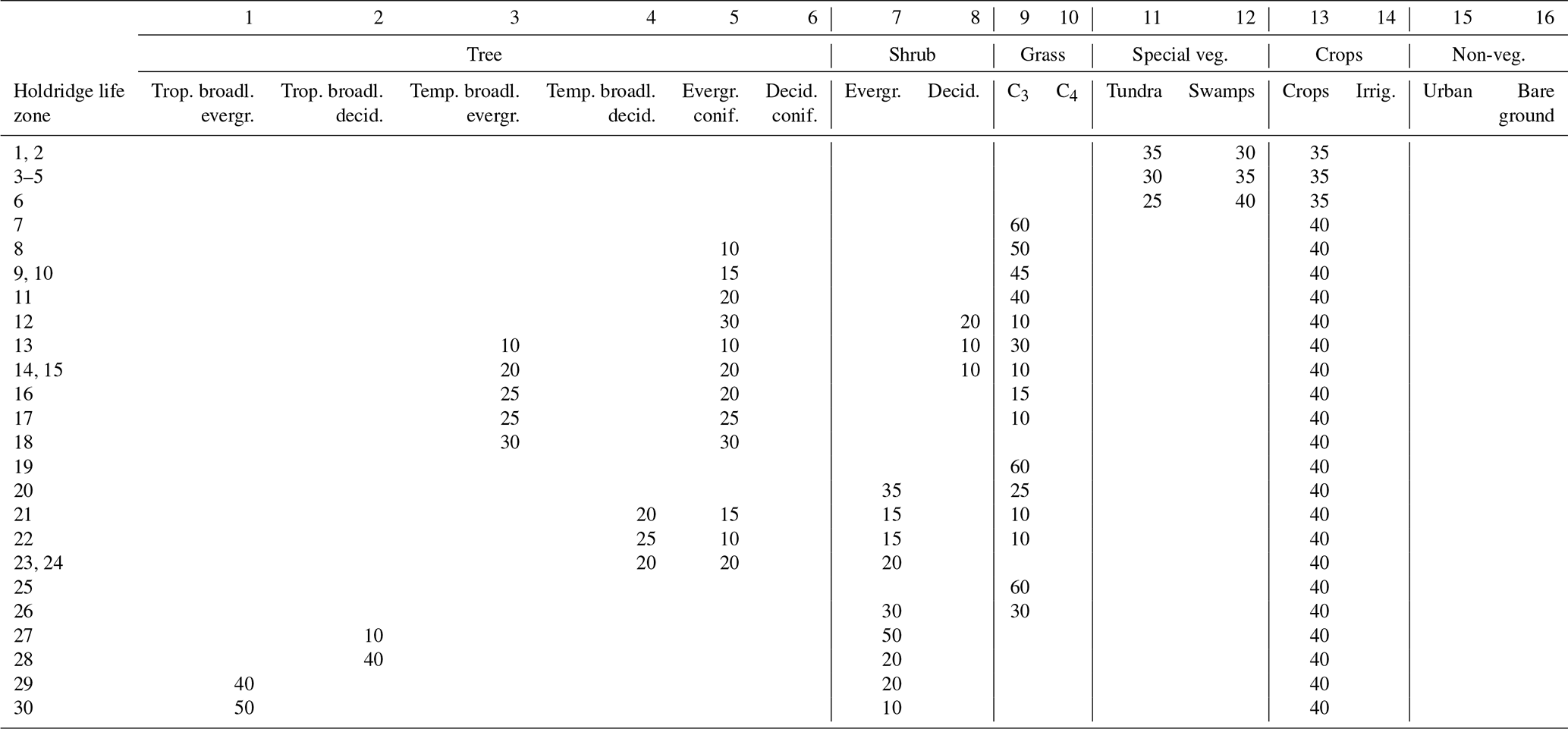
A CWT (Sect. 3) is created for each of the 37 ESA-CCI LC classes. Since the table has three dimensions (land cover class, HLZ and PFT), it was necessary to prepare the individual tables that include unique translations for each HLZ. For example, Table 1 shows the CWT for LC class 40 – Mosaic natural vegetation (tree, shrub, herbaceous cover) (>50 %)/cropland (<50 %) – where the numbers of the HLZs in the first column correspond to the HLZ numbers in Fig. 2. For each HLZ in the first column, LC class 40 is translated into fractions of the LANDMATE PFTs. For the example class that means an increasing tree fraction from the boreal to tropical HLZs and a change in tree species composition which makes the whole PFT fraction composition per pixel regionally adjustable. Each pixel of the map that contains one specific ESA-CCI LC class is translated to contain multiple PFT fractions representing the properties of multiple LC types, such as roughness length, albedo or leaf area index. These multiple properties can further be implemented in an RCM. Depending on the ability of the RCM, multiple fraction properties or an average of the properties are passed on to the overlaying and underlaying layers, where the average of all PFT fraction properties is still a more accurate representation of LC than the properties of only one LC class. An example of the implementation of PFT fractions in an RCM is given by Wilhelm et al. (2014), where the use of PFTs within the RCM REMO is described.
Table 1Cross-walking table for ESA CCI LC class 40 – Mosaic natural vegetation (tree, shrub, herbaceous cover) (>50 %)/cropland (<50 %).
The translation process is based on Wilhelm et al. (2014), where the translation of the Global Land Cover (GLC) 2006 into the 16 REMO-iMOVE PFTs is described. Since the nomenclatures of GLC 2006 and ESA-CCI LC are similar and based on the same classification system, some of the CWTs were initially adopted from Wilhelm et al. (2014). For the more diverse ESA-CCI LC classes, new CWTs need to be created. The new CWTs follow the translation of Poulter et al. (2015) (ESA POULTER) but were carefully revised and modified during the process. After application of the CWP, an additional map of potential C3 and C4 grass vegetation (North American Carbon Program Multi-scale Synthesis and Terrestrial Model Intercomparison Project – NACP MsTMIP, Sect. 2.2.6) is used to divide the grass PFT fractions. The quality of the LANDMATE PFT dataset is finally assessed by comparison to a comprehensive ground truth database (LUCAS land use and land cover survey, Sect. 4).
2.2 Datasets and concepts
2.2.1 ESA-CCI LC
The ESA-CCI provides continuous global land cover maps (ESA-CCI LC) at ∼ 300 m horizontal grid resolution. The ESA-CCI LC maps are available for download in annual time steps for the years 1992–2018 (ESA, 2017a). The classification of the LC maps follows the United Nations Land Cover Classification System (UN-LCCS) protocol (Di Gregorio, 2005) and consists of 22 level-1 classes and 14 additional level-2 classes, which include regional specifications. More information on ESA-CCI LC data processing can be found at http://maps.elie.ucl.ac.be/CCI/viewer/download/ESACCI-LC-Ph2-PUGv2_2.0.pdf (last access: 4 April 2022). An overview of the satellite missions involved in the production of ESA-CCI LC is given in Table 2. Besides systematic global validation efforts (ESA, 2017a; Hua et al., 2018), a few regional approaches investigated the quality of ESA-CCI LC over Europe (Vilar et al., 2019; Reinhart et al., 2021a).

1 MEdium Resolution Imaging Spectrometer Full Resolution/Reduced Resolution (ESA, 2006). 2 Surface reflectance. 3 Advanced Very-High-Resolution Radiometer (Hastings and Emery, 1992). 4 SPOT Vegetation satellite programme (Maisongrande et al., 2004). 5 Project for On-Board Autonomy – Vegetation (Dierckx et al., 2014). 6 Ocean and Land Colour Instrument (OLCI) and Sea and Land Surface Temperature Radiometer (SLSTR) (Donlon et al., 2012).
2.2.2 E-OBS climate data
The E-OBS dataset (Cornes et al., 2018) is a daily gridded observational dataset derived from station observations from European countries covering the period from 1950 to 2020. The point observations are interpolated using a spline method with random perturbations in order to produce an ensemble of realizations. For the creation of the HLZs that are used for the conversion of ESA-CCI LC classes to PFTs (Sect. 2.2.5), the ensemble mean of the 2 m temperature (TG) and precipitation (RR) on a regular 0.1∘ grid from E-OBS Version 19.0e is used. It covers most of Europe, some parts of the Middle East and a narrow strip of northern Africa.
2.2.3 CRU
The CRU TS 4.03 dataset is a global gridded high-resolution climate dataset based on station observations produced and maintained by the CRU of the University of East Anglia (Harris et al., 2014). The dataset provides global monthly means of climate parameters at 0.5∘ resolution from 1901 to 2019. In order to achieve the target resolution of 0.1∘ for the global LANDMATE PFT maps, the CRU climate data are downscaled using bilinear interpolation. Following Hoffmann et al. (2016), distance-weighted interpolation was applied to the atmospheric observation dataset CRU to extrapolate the climate data to the coastlines of the ESA-CCI LC maps in order to compensate for the different land–sea masks of the products. The CRU climate dataset was used within this application for regions where E-OBS is not available. The bilinear interpolation of E-OBS caused minor issues on coastlines and small islands all over the research area, where this interpolation method was not able to correctly account for the resolution differences of the 0.1∘ E-OBS and 0.018∘ LANDMATE PFT land–sea masks, respectively. The issue caused by the large resolution difference is fixed with a preceding extrapolation of the climate data along coastlines and islands in the LANDMATE PFT map Version 1.1 that is currently being prepared. Since the interpolation issue only affected a negligible number of LANDMATE PFT cells, the validation measures are not affected by this issue in a noticeable way.
2.2.4 Holdridge life zones
The Holdridge life zone concept was initially developed in 1967 (Holdridge, 1967) to define all divisions of the global biosphere, depending on the relation of biotemperature (average of monthly temperature above 0∘C; since plant activities are idle below freezing, all values below 0∘C are adjusted to 0∘C), mean annual precipitation and the ratio of potential evapotranspiration to mean annual precipitation. By combining threshold values of biotemperature and annual rainfall, the 38 HLZs are created (Table 3). In the present analysis, the subtropical and warm temperate as well as polar and subpolar HLZs are merged. Through the merging of the aforementioned HLZs, 30 individual HLZs in total are available for the creation of the European HLZ map (Fig. 2).
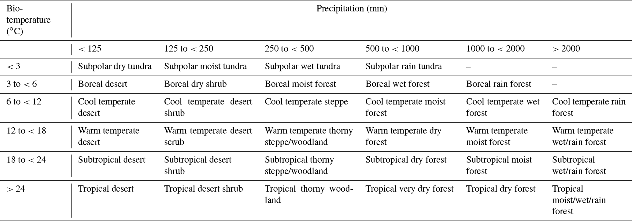
The dynamic character of the specific quantitative ranges of the long-term means of the utilized climate parameters makes the HLZ classification more flexible than other available global ecosystem classifications and therefore makes the HLZs most suitable for the application presented in this article. In addition, the requirement for input data is relatively low.
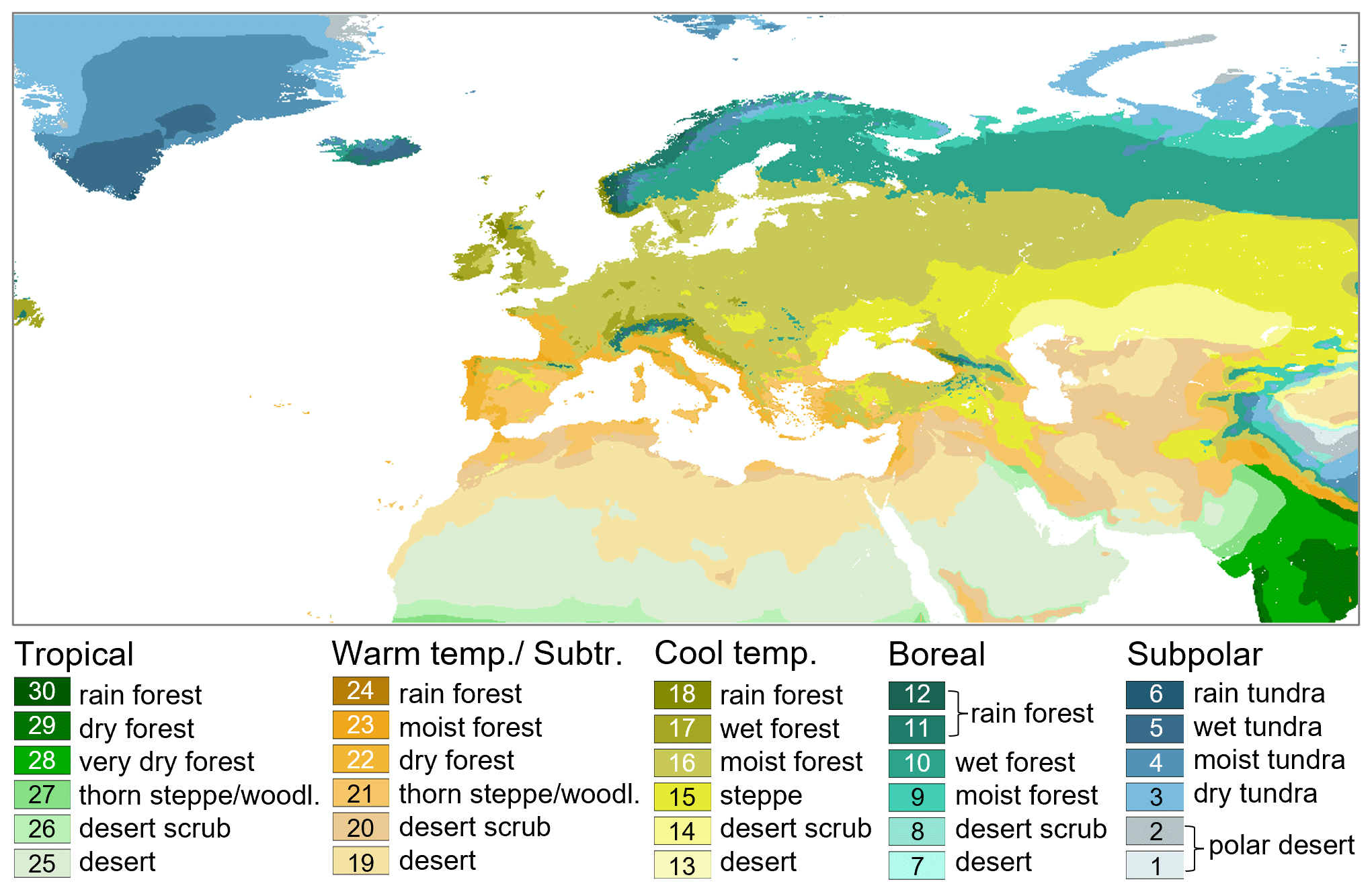
Figure 2Holdridge life zone map for the extent of LANDMATE PFTs.
In the past, the HLZ concept was not only found to be useful for global applications, but was also successfully implemented, especially for regional mapping approaches, due to its ability to capture regional climate features with the support of bioclimatic variables (Daly et al., 2003; Tatli and Dalfes, 2016). Further, the HLZ concept was used for LULC change predictions, such as land use impact assessments, related to current and future climate change scenarios (Chen et al., 2003; Skov and Svenning, 2004; Yue et al., 2006; Saad et al., 2013; Szelepcsényi et al., 2018). With the implementation of climate data through the HLZ concept, the resulting PFT maps become more detailed and can be customized to individual regions without losing global consistency.
2.2.5 Plant functional types
Figure 3 shows the LANDMATE PFTs that are based on the PFTs introduced by Wilhelm et al. (2014). The implementation of an irrigated cropland PFT (PFT 14) that is currently being developed within the HICSS project LANDMATE will be implemented in a later version of the dataset. In the initial version that is presented in this article, all cropland proportions are assigned to the cropland PFT (PFT 13).
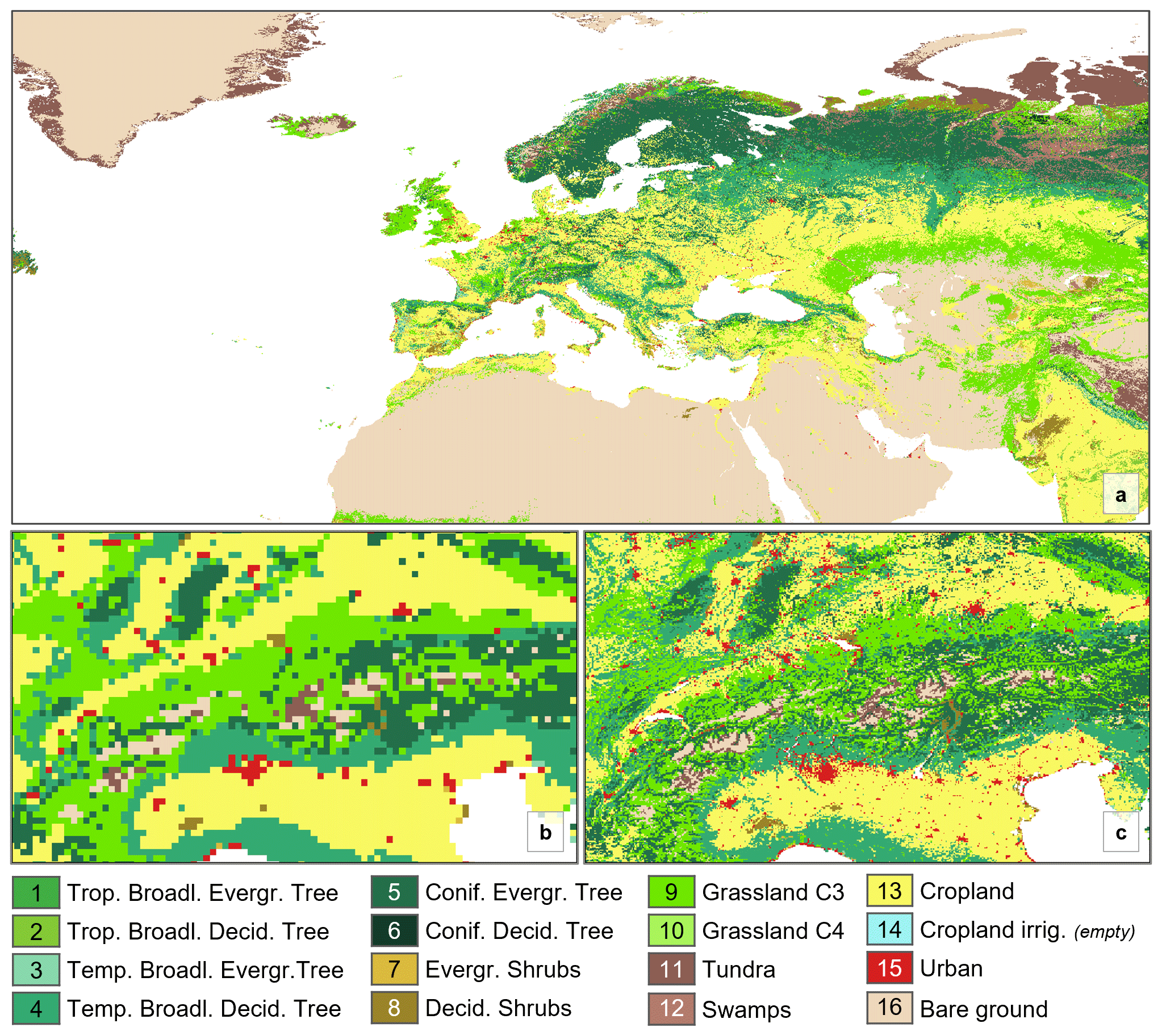
Figure 3LANDMATE PFT map for Europe for 2015 (a). Below a map section of the Alpine region shows an example of the resolution difference between LANDMATE PFT 0.1 (b) and LANDMATE PFT 0.018 (c). LANDMATE PFT 0.018 is used in the present accuracy assessment. For improved visualization, all maps show the majority PFT per grid cell. The irrigated cropland PFT (14) is not used in this map. More information is given in Sect. 3.4.
2.2.6 Potential C4 grass fraction NACP MsTMIP
The initial land cover map from the ESA-CCI LC does not provide a distinction between C3 and C4 grassland. The focus of the present approach is the improvement of representation of the biophysical properties of LC types. Since the distinction between C3 and C4 grasses is rather important for biochemical properties, such as the carbon cycle, the decision was made to use a pre-existing, external product for the spatial distinction between C3 and C4 grasses. The map from the NACP MsTMIP (Wei et al., 2014) is constructed based on the synergetic land cover product (SYNMAP) by Jung et al. (2006). SYNMAP is a combination of multiple high-resolution LULC products using a fuzzy agreement approach. The NACP MsTMIP map uses the grassland fractions from the SYNMAP product. The potential C4 grass distribution is generated by Wei et al. (2014) by employing the well-established method introduced by Still et al. (2003), which is based on the growing season temperature and rainfall in combination with present climate conditions from the global CRU-NCEP dataset. The potential C4 grass map is provided on a 0.5∘ horizontal grid for the period from 1801 to 2010. For the preparation of LANDMATE PFT the NACP MsTMIP map of 2010 is used. The LANDMATE PFT grass fraction is split up into C4 and C3 grasses by multiplying grassland by the potential C4 vegetation fraction and for C3 grass (1 – potential C4 vegetation fraction), respectively.
The spatial distribution of C3 and C4 grasses is not evaluated in the present approach due to the lack of information in the reference dataset. Through the use of the state-of-the-art NACP MsTMIP map, the highest possible quality of C3 and C4 grass distribution given in the LANDMATE PFT map is ensured.
2.3 LUCAS – land use and land cover survey
The harmonized LUCAS in situ land cover and use database for field surveys from 2006 to 2018 (d’Andrimont et al., 2020) is the most consistent ground truth database for the European continent. The survey was carried out at 3-yearly intervals between 2006 and 2018. The systematic sampling design of the survey consists of a theoretical, regular grid over the European continent with ∼ 2 km grid size. The reference point locations are the corner points of the theoretical grid. Not all locations within the survey were easily accessible. Therefore, the survey is supported by in situ photo interpretation, in-office photo interpretation and satellite data in the latest time steps 2015 and 2018 (Table 4). However, the main proportion of the reference points was recorded through location visits at all time steps, which makes this land survey the most reliable and consistent ground truth database for Europe.
Table 4Number and recording method of reference points in the LUCAS land cover and use database per time step.

1 Photo interpretation close to the reference location. 2 Photo interpretation with supporting data, such as satellite images. 3 Ground truth.
The extent of the LUCAS survey was increased over time. The 2006 survey covered 11 countries, while the 2018 map covers large parts of the European continent, with 28 countries. Throughout the survey, the ground truth data were continuously checked for quality and plausibility. For the accuracy assessment of the LANDMATE PFT map, the ground truth points of the year 2015 are employed (Sect. 4). In order to avoid confusion between the FPS LUCAS and the LUCAS ground truth dataset, the latter will be further referred to as ground truth survey or GT-SUR.
The CWP from ESA-CCI LC classes to PFTs presented in this article is based generally on (1) the translation introduced by Poulter et al. (2015) and (2) the translation by Wilhelm et al. (2014). Both translations are not just combined with each other, but are also modified using additional data. The following sections introduce the PFTs of LANDMATE PFT aggregated into general LULC types and give an overview of the decisions on modifications that are made during the production process based on literature and additional data.
3.1 Trees and shrubs, tropical and temperate | PFTs 1–8
The LANDMATE PFTs are more diversified regarding tree PFTs than the generic ESA POULTER PFTs. While the generic ESA POULTER PFTs have four shrub PFTs, the LANDMATE dataset has only two, while the tree PFT count was increased to six. The increase in tree PFT diversity is done in order to address the strong biogeophysical impacts of forested areas on regional and local climate, such as decreased albedo and increased roughness length (Bright et al., 2015). The effects of forested areas on near-surface climate are distinctively different to the effects of shrub- or grass-covered areas and are also highly dependent on tree species composition and latitudinal range (Bonan, 2008; Richardson et al., 2013). Another reason for the six tree PFTs is the intended use of the PFT maps in RCMs. In the land surface models (LSMs) of current-generation RCMs, a distinction is rather made between different tree or tree community types than between different shrub types. Therefore, and with regard to the implementation process that needs to be done for each RCM individually, an increase in the number of tree PFTs and a decrease in the number of shrub PFTs are considered to be convenient. Accordingly, the tree and shrub proportions were distributed following both the needleleaf and broadleaf definitions of the ESA-CCI LC classes as well as the HLZ map, where the HLZ map was decisive for an assignment of forest proportions to the temperate or tropical tree PFT, respectively. Following a comparison to different forest datasets over Europe (not shown), the tree proportions in the translation of the mixed land cover classes, e.g. class 61 – Tree cover, broadleaved, deciduous, closed (>40 %), are increased to be in line with the indicated overall forest amount over Europe.
3.2 Grassland | PFTs 9 and 10
The generic ESA POULTER PFTs include a natural grassland and a managed grassland PFT to include grassland and cropland, respectively. The LANDMATE PFTs include two grassland PFTs, distinguishing between C3 and C4 grass. The contrasting photosynthetic pathways and therefore contrasting synthetic response to CO2 and temperature determine specific ecosystem functions for both PFTs, respectively. The main differences are found in global terrestrial productivity and water cycling (Lattanzi, 2010; Pau et al., 2013). The translation from the LULC classes that contain grassland proportions into C3 or C4 grass PFTs, respectively, is supported by a map of potential C4 vegetation by Wei et al. (2014), where the potential global distribution of C4 is estimated using bioclimatic parameters (Sect. 2.2.6).
3.3 Tundra and swamps | PFTs 11 and 12
The specific vegetation PFTs tundra and swamps are treated individually in LANDMATE PFT. Tundra is mostly used for the polar and subpolar HLZs, where the climatic conditions require a clear distinction of the land surface properties from the boreal and temperate regions regarding exchange and feedback processes with the atmosphere (Thompson et al., 2004). Chapin et al. (2000) further suggest a differentiation of vegetation composition within these northern vegetation communities, which can also be realized using the introduced CWP. The swamp PFT is mostly used for translating the ESA-CCI LC mosaic tree/shrub/herbaceous classes and also partly for the flooded tree cover classes in most of the HLZs. Swamps occur mainly in the boreal and polar regions in the European domain.
3.4 Cropland | PFTs 13 and 14
Currently, two cropland PFTs are defined in the LANDMATE PFT map. The cropland PFT (PFT 13, Fig. 3) includes all managed, agricultural land surface proportions. The uncertainties of the translation of the ESA-CCI cropland classes and mixed cropland classes into the cropland PFTs were investigated by Li et al. (2018), where the comparison of LULC change in the ESA POULTER PFT maps against other LULC products showed inconsistencies between global trends and geographical patterns between the products. However, Li et al. (2018) provide a modified CWT that was adjusted with regard to an improved knowledge base on how to translate LULC classes into PFTs for climate models. Particular focus is laid on mosaic classes and the sparsely vegetated classes, of which numerous appear in ESA-CCI LC. Therefore, the CWP from Li et al. (2018) for cropland is adopted in the present CWP.
The irrigated cropland PFT (PFT 14, Fig. 3) is currently empty in the LANDMATE PFT map Version 1.0. This decision is made following intense research on available irrigation information. The ESA-CCI LC map that is used as initial input contains an “irrigated cropland” class, but this information was not used in the process. The investigation on irrigated areas included the comparison of ESA-CCI LC to other products that are available, such as the irrigation map from the FAO (Siebert et al., 2005). Although the ESA-CCI LC quality assessment shows very good agreement of the ESA-CCI LC irrigated cropland with the validation database (ESA, 2017a), the comparison showed considerable differences between the products. The success of detection of irrigated areas is highly dependent on the correct detection of the crop types to infer the water needs of the respective crops, on atmospheric and environmental conditions and on the availability of multi-temporal, high-resolution imagery (Bégué et al., 2018; Karthikeyan et al., 2020). Further, most remote sensing applications depend highly on ground truth data and local knowledge. Applications using different satellite imagery to detect agricultural management practices, such as irrigation, are only successfully tested and applied in local spatial units (Rufin et al., 2019; Ottosen et al., 2019). Therefore, the irrigated cropland PFT remains unoccupied for now. Nevertheless, PFT 14 is defined within LANDMATE PFT Version 1.0 for the purpose of adding irrigated LULC fractions in the future. For the long-term LUCAS LUC dataset (Hoffmann et al., 2021), which is extended backward and forward based on the LANDMATE PFT map for Europe 2015, irrigated cropland areas are already implemented following the irrigated area definition of the Land Use Harmonization (LUH2) dataset (Hurtt et al., 2011).
3.5 Non-vegetated | PFTs 15 and 16
The non-vegetated PFTs in the LANDMATE PFT dataset are urban and bare. The urban grid cells from ESA-CCI LC are directly translated into urban fractions for all HLZs in the CWP. The same applies for all bare ground proportions that are translated fully into the bare PFT. In addition, the ESA-CCI LC mixed classes are split up, and the bare ground proportions within the mixed classes are added to the bare PFT. The explicit treatment of urban areas and especially differentiation from bare ground provides the possibility of resolving urban surface characteristics in RCMs. The treatment of urban areas as a slab surface or as an equal to rock surface as done in several RCM approaches cannot account for the complex biogeophysical processes associated with an urban agglomeration (Daniel et al., 2019; Belda et al., 2018). Due to the distinction of the two surface types, the LANDMATE PFT map can be used for impact studies with an urban focus.
3.6 Water, permanent snow and ice
The LANDMATE PFTs do not include individual PFT definitions for water and snow/ice, respectively. Regarding the water representation, most currently used RCMs utilize a land–sea mask to account for oceans and inland water areas. Therefore, an explicit definition of water as an individual PFT has not been implemented. Consequently, all water fractions such as marine water, lakes and rivers are set to no data. In the present translation, the snow/ice grid cells from ESA-CCI land cover are translated into a bare PFT following Wilhelm et al. (2014).
The LANDMATE PFT map is based on the ESA-CCI LC map which was quality checked and compared to similar LULC products on a global (ESA, 2017b; Yang et al., 2017; Hua et al., 2018; Li et al., 2018) and regional level (Reinhart et al., 2021a; Vilar et al., 2019). However, the translation from LULC classes into PFTs necessarily results in a change in the map. The final product, the LANDMATE PFT map, is intended to be used in RCMs, which means the quality of the final product must be assessed in addition to the available quality assessments of the initial ESA-CCI LC map. In order to overcome the resolution difference, which is non-negligible between LANDMATE PFT and the reference data GT-SUR, the LANDMATE PFT map is prepared at 0.018∘ horizontal resolution, which corresponds closely to the 2 km theoretical grid of GT-SUR.
The design of such a quality assessment of a large-scale map product is not trivial, especially since the map product itself and the reference data are often different in structure and nomenclature, given that ground truth reference data are mostly collected as point data and independently of the assessed map product (Foody, 2002; Wulder et al., 2006; Olofsson et al., 2014). In order to produce reliable quality information for LANDMATE PFT, the present assessment follows closely the well-established good-practice recommendations. Nevertheless, adjustments are done to account for the fractional structure of LANDMATE PFT. Section 4.2 provides additional information on the requirements of a good-practice accuracy assessment, the key components and the selected sampling design and metrics.
4.1 Research area
The coverage of GT-SUR in the year 2015 includes 28 countries which are highlighted in dark grey in Fig. 4.

Figure 4Coverage of the reference GT-SUR over the European continent (a). As an example for the whole research area (b) shows the GT-SUR point coverage (and LULC group representation) of one grid cell of the auxiliary 2.5∘ grid.
The total number of GT-SUR points for 2015 is 340 143. Out of these points, 338 619 points (∼ 99.55 %) are covered with valid LANDMATE PFT grid cells of the assessed LULC types and can be used in the analysis. Countries located within the contiguous area but missing in the assessment are Switzerland, Norway, the Russian Kaliningrad Oblast, Bosnia and Herzegovina, Montenegro, Albania, Serbia, Kosovo, North Macedonia, and Belarus. Figure 4 also shows the 2.5∘ grid that was used for the analysis of the accuracy assessment results (Sect. 5). Due to the fine scale and the high number of points over the whole research area, the visualization of the spatial analyses on a continental scale is challenging. Therefore, the research area is overlayed with a 2.5∘ grid (as shown in Fig. 4). While the results are presented in these 2.5∘ grid units, the results are calculated for each point within one unit and then aggregated. For example, in a 2.5∘ grid unit containing 1000 pairs of LANDMATE PFT cells and GT-SUR points, 50 % overall accuracy is achieved when 500 pairs agree on the LC type. The overall and class-wise accuracy results for all points within each 2.5∘ grid cell are aggregated in order to identify large-scale spatial quality differences for the analysed LULC types. In order to give information on the relevance of the accuracy metrics, the number of LANDMATE PFT–GT-SUR pairs for each LULC type per grid cell are displayed alongside the accuracy figures in Sect. 5.
4.2 Accuracy assessment – background and design
The key components of the accuracy assessment of a large-scale land cover product are objective, sampling design, response design and the final analyses and estimation (Wulder et al., 2006). All of the key components have great impact on the quality of the assessment and, further, on the final metrics, especially in the present assessment, where reference and assessed dataset differ widely in structure. LANDMATE PFT is a gridded dataset with fractional LULC classes but no information on the subgrid location within the grid cell. Other than that, the points of GT-SUR have fixed locations expressed through exact coordinates but no (exact) information on the spatial extent of this class. Another challenge is the fractional structure of LANDMATE PFT itself, where one unit (grid cell) possibly contains multiple fractions. Therefore, the design of the accuracy assessment needs to be customized to the objective, which is to determine the overall quality of the LANDMATE PFT map for Europe 2015 as well as the quality of individual LULC type representation within the map in order to derive recommendations for the use of LANDMATE PFTs in RCMs.
When it comes to the sampling design, sampling size, spatial distribution of the respective sample and the representation of each LULC type or class within the sample are crucial for producing reliable quality information about a LULC product (Stehman, 2009). The collection of ground truth data is a rather expensive procedure regarding time and money, which needs to be considered during the process. However, in the present assessment we are able to rely on an existing ground truth database containing over 340 000 records, which eliminates the possible issue of a too small reference database. It is also known that all assessed LULC types are represented in a sufficiently high number (Table 6). Nevertheless, the present assessment is a special case situation, with every unit of LANDMATE PFT containing more than one LULC type potentially. Therefore, the subsets are selected through application of a filter to capture the map accuracy in a way that accounts for the fractional structure within the grid cells in the LANDMATE PFT map (see Sect. 4.2.1).
The response design deals with the spatial support regions (SSRs) and the labelling protocol or classification harmonization. The SSR is a buffer region around a sampling unit that is selected to account for small-scale landscape heterogeneity that is likely not captured by larger-scale map products. In the present case, the sampling design is selected in a way that the grid cells of LANDMATE PFT serve as SSRs for each GT-SUR point. A fraction is not located precisely at one location within the respective grid cell but is evenly distributed over the whole grid cell. Assuming the uniformly distributed fraction can occur in small patches or in one large patch within the grid cell, the whole grid cell is defined as an SSR for the respective LULC type. The labelling protocol needs to be determined to deal with the different legends of the reference and the assessed map. The harmonization of legends is selected with regard to the objective of the respective assessment, as in this case, to provide information about the quality of representation of the most dominant LULC types in LANDMATE PFT. The labelling protocol used in the present assessment is summarized in Table 5.
The analyses and estimation used are error matrices that give an overview of the overall and LULC type-wise accuracy of the LANDMATE PFT map. For both resolutions of LANDMATE PFT, the error matrices and the resulting accuracy measures overall accuracy (OA), producer's accuracy (PA) and user's accuracy (UA) are calculated, where PA and OA are calculated group-wise. The error matrix is a cross-tabulation between map and reference of the size q×q, where q stands for the number of land cover classes or groups. The map classes are placed in the rows and the reference classes in the columns so that the diagonal of the matrix gives the sum of the correctly classified map units. The off-diagonal cell values represent the disagreement between the map and the reference. The overall accuracy is calculated according to Eq. (1):
The sum of the agreeing diagonal elements nii of all LULC types is divided by the number of all observations n. The PA represents the accuracy from the view of the map producer. The PA stands for the probability that a LULC feature in the reference is classified as the respective feature by the map. The PA is calculated using Eq. (2), where the number of correctly classified units per LULC type nii is divided by the total number of LULC type occurrences of the reference n+i:
While the PA gives the proportion of features in the reference that are actually represented as those in the produced map, the UA is the accuracy from the perspective of the map user. It is the probability of a feature classified as such in the map being actually present in the reference. The UA is calculated using Eq. (3), where the number of correctly classified pixels nii per LULC type is divided by the row sum :
4.2.1 Dataset harmonization and filter
The quality assessment is done by assigning the PFT type with the maximum fraction per grid cell to the GT-SUR points located within the respective grid cell. The classifications of both datasets are harmonized as shown in Table 5, where the focus is laid on the main LULC types in order to make the comparison as detailed as possible but also to be able to produce reliable and robust results for the RCM community.
Table 5Classification harmonization between the LANDMATE PFT map and GT-SUR.
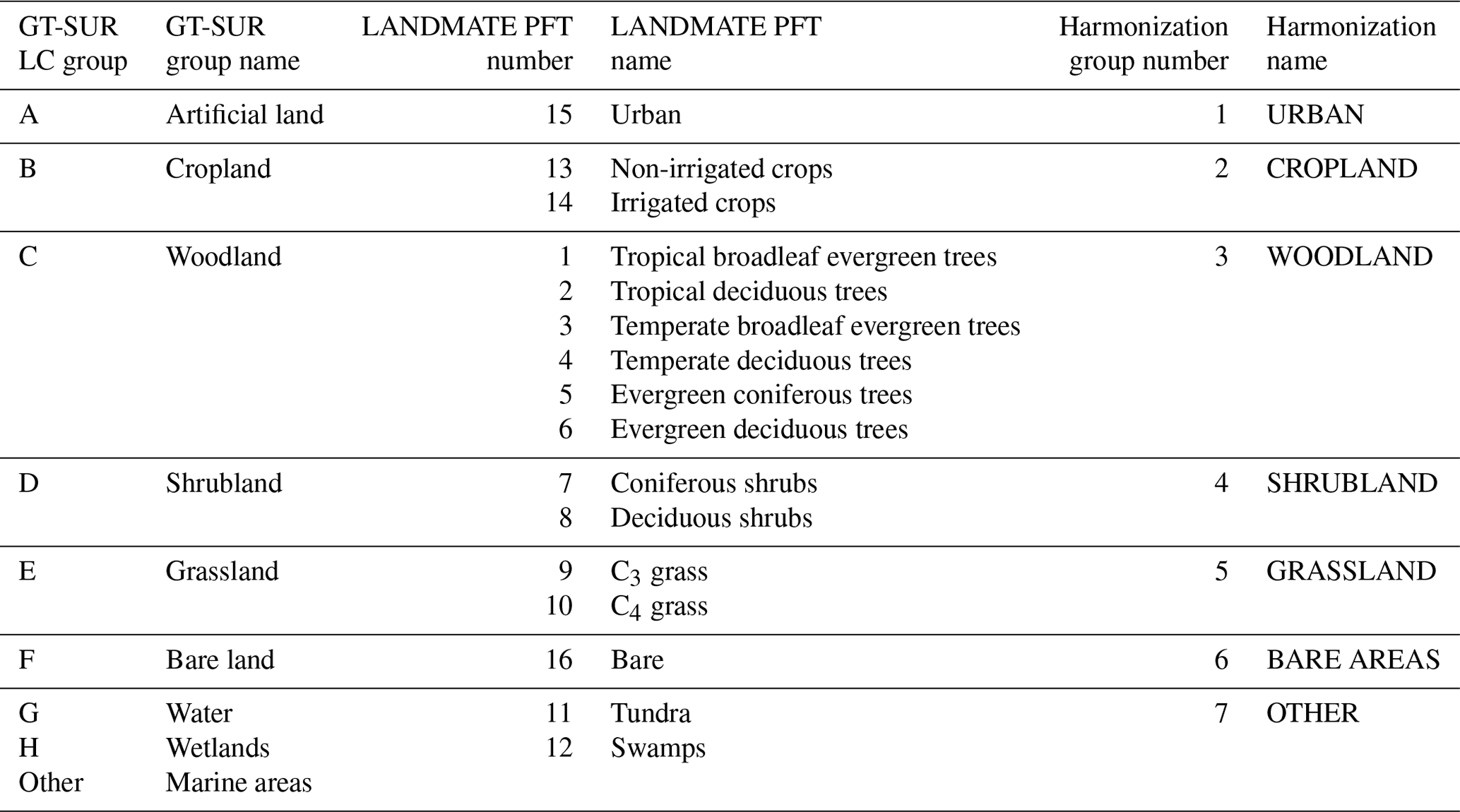
The LULC types URBAN, CROPLAND, WOODLAND, SHRUBLAND, GRASSLAND and BARE AREAS are harmonized without applying modifications to the classifications. The LANDMATE PFTs can easily be grouped or directly adopted, while the GT-SUR level-1 classification (letters A–H) is completely adopted into the harmonized groups. In general, RCMs implement a dedicated land–sea mask to determine aquatic areas for both inland and marine water. Therefore, the categories Water and Marine areas are not further analysed. Since the LULC types Tundra and Swamps (LANDMATE PFT) and Wetlands (GT-SUR) cannot be harmonized with sufficient agreement with the GT-SUR LULC type definitions, the LULC types are also not further analysed in the assessment. Thus, the LULC types Water and Marine areas and Wetlands (GT-SUR) and Tundra and Swamps (LANDMATE PFT) are merged into the LULC type OTHER. Although the group cannot be evaluated regarding the quality of the LANDMATE PFT map, the group needs to be involved in the assessment to keep the numbers in the assessment correct and reliable for all other groups. However, as is shown in Table 6, only a minor number of points/cells is affected.
Both datasets are provided in a regular Gaussian grid (WGS84 EPSG:4326) so that no reprojection of the datasets needs to be done for the comparison.
The LANDMATE PFT dataset includes multiple LULC fractions per grid cell. Accordingly, the area proportion of the dominant LULC type varies widely and thus the likelihood that the GT-SUR point sample falls within this area. The grid cells are grouped by minimum coverage of the dominant LULC type from 0.1 to 1, where 0.1 means a minimum coverage of 10 % and 1 means full coverage of the dominant LULC type. The coexisting fractions are not located in particular parts within a grid cell but are equally distributed, while the GT-SUR points have fixed locations on the map. With the applied grouping of the cells dependent on the minimum coverage of the dominant LULC type, the influence of grid cell heterogeneity on accuracy metrics is investigated within the assessment.
Besides the total number of LANDMATE PFT cells in the analysis, diversity among the represented LULC types is important. The right column of Table 6 shows the number of LANDMATE PFT cells where the respective LULC type (left column) is dominant. The table is not grouped by minimum coverage but by LULC type and shows that each assessed LULC type is represented in a sufficiently high number when only the cells with dominant coverage (regardless of the total proportion) are considered for each LULC type.
Table 6General information on data in the comparison.
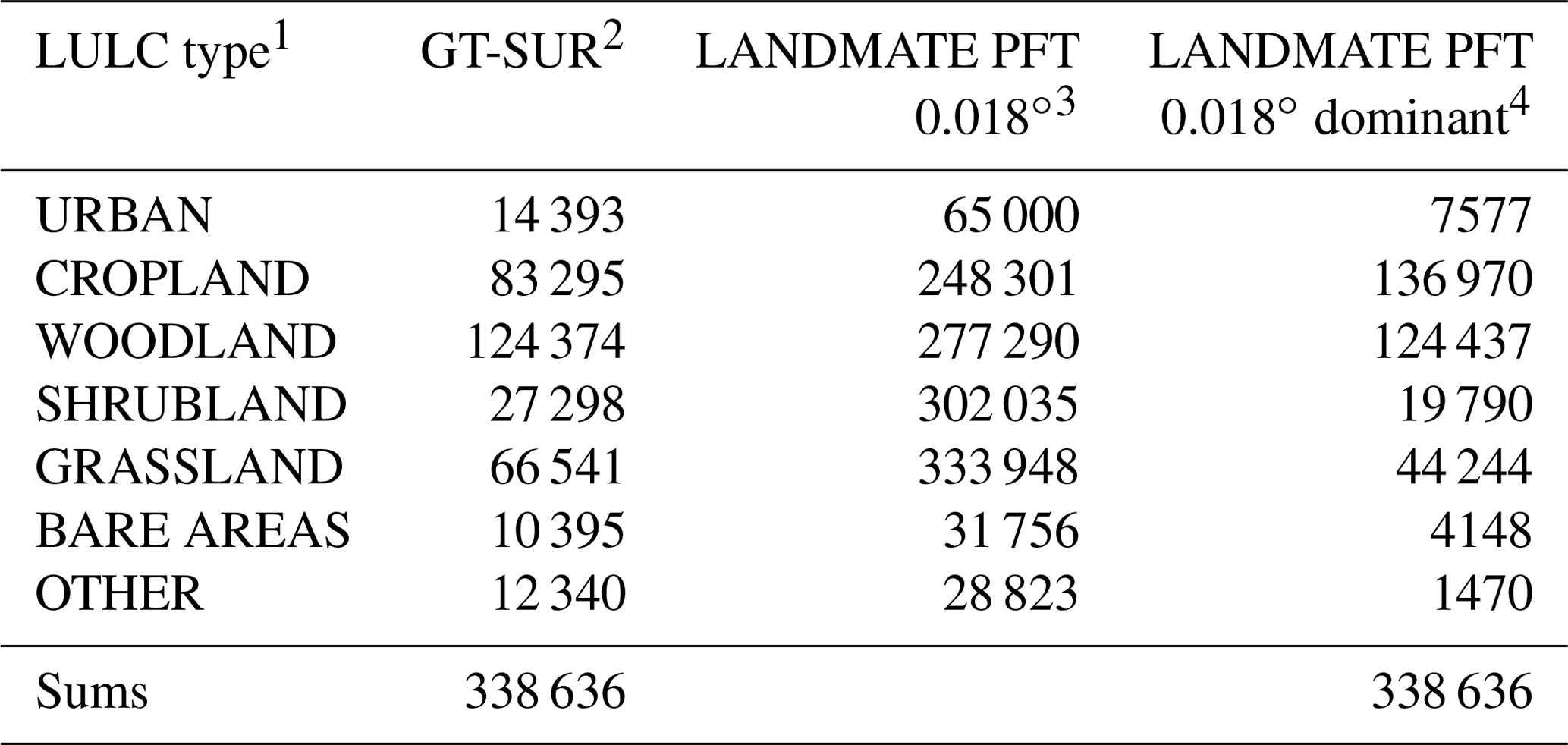
1 LULC type analysed in the quality assessment. 2 Number of GT-SUR points per LULC type. 3 Total number of grid cells in LANDMATE PFT that have a share >0 % of the respective LULC type. 4 Number of cells where the LULC type is dominant in LANDMATE PFT 0.018∘.
In order to show the impact of the grid cell heterogeneity of LANDMATE PFT, the agreement of LANDMATE PFT with the reference GT-SUR is investigated for each threshold for minimum coverage (0.1–1) of the dominant LULC type. For visualization of the spatial analysis, the point count and percentage agreement with the reference dataset are aggregated per 2.5∘ cell of the auxiliary grid, which was established as most useful for visualization of the results. Nevertheless, the comparison of LANDMATE PFT to GT-SUR is done at cell level for the whole research area. All resulting confusion matrices for the assessed LC types at cell level are available in Appendix B.
In order to be able to capture the spatial distribution of the quality of the LULC type representation within LANDMATE PFT, the assessed cells must be distributed well over the research area and contain a sufficiently large cell count of each LULC type. Figure 5 shows the distribution and count of cells grouped by threshold for minimum coverage. The maps show that the groups with a threshold lower than 0.7 are distributed very well over the research area. Each region is covered with a sufficient number of LANDMATE PFT grid cells that can be compared to the respective GT-SUR points. The 0.8 group shows a quite patchy pattern and a strongly decreasing sample number in northern Europe. For the 0.9 group, the patchy pattern and low number of cells per 2.5∘ grid cell spread over the whole research area. While the 0.9 group could still be used for evaluation of LANDMATE PFT for limited regions in Europe, the group only containing cells with 100 % coverage of one LULC type (map 1) is clearly not evaluable due to the overall small cell count (<1500). Figure 6a gives an overview of the cell count per group for each individual LULC type.
For CROPLAND, WOODLAND and GRASSLAND, the threshold for minimum coverage of the respective dominant LULC type has a strong influence on the total cell count within each group, while for URBAN and BARE AREAS, the cell count remains similar up to the 0.6 group. For SHRUBLAND, the cell count decreases strongly from the 0.4 group upwards. The curve characteristics suggest that the LULC types CROPLAND, WOODLAND, and GRASSLAND have a higher proportion of cells with a relatively low dominant coverage, but since they are the three most populated LULC types overall (see Table 6), the proportions are comparable to the other three groups.
Figure 6b shows the highest UA for WOODLAND and the lowest for SHRUBLAND, while all the other LULC types range in between. The threshold for minimum coverage of the individual LULC types has slightly more influence on the UA than on the PA of LANDMATE PFT, where the UA increases towards the groups with higher cell homogeneity.
Figure 6c shows the PA for all LULC types dependent on the threshold for minimum coverage of the dominant LULC type, including the overall accuracy for all LULC types together (dark grey line). While the overall accuracy is relatively independent of the threshold for minimum coverage, some LULC types are affected. For WOODLAND, PA decreases rapidly for the 0.8 group. Considering that the cell count for this group does decrease noticeably from 0.7 to 0.8 (Fig. 6a), the low PA is likely a result of this low cell count. The PAs for GRASSLAND and SHRUBLAND remain almost constant but at a lower level compared to the other groups.
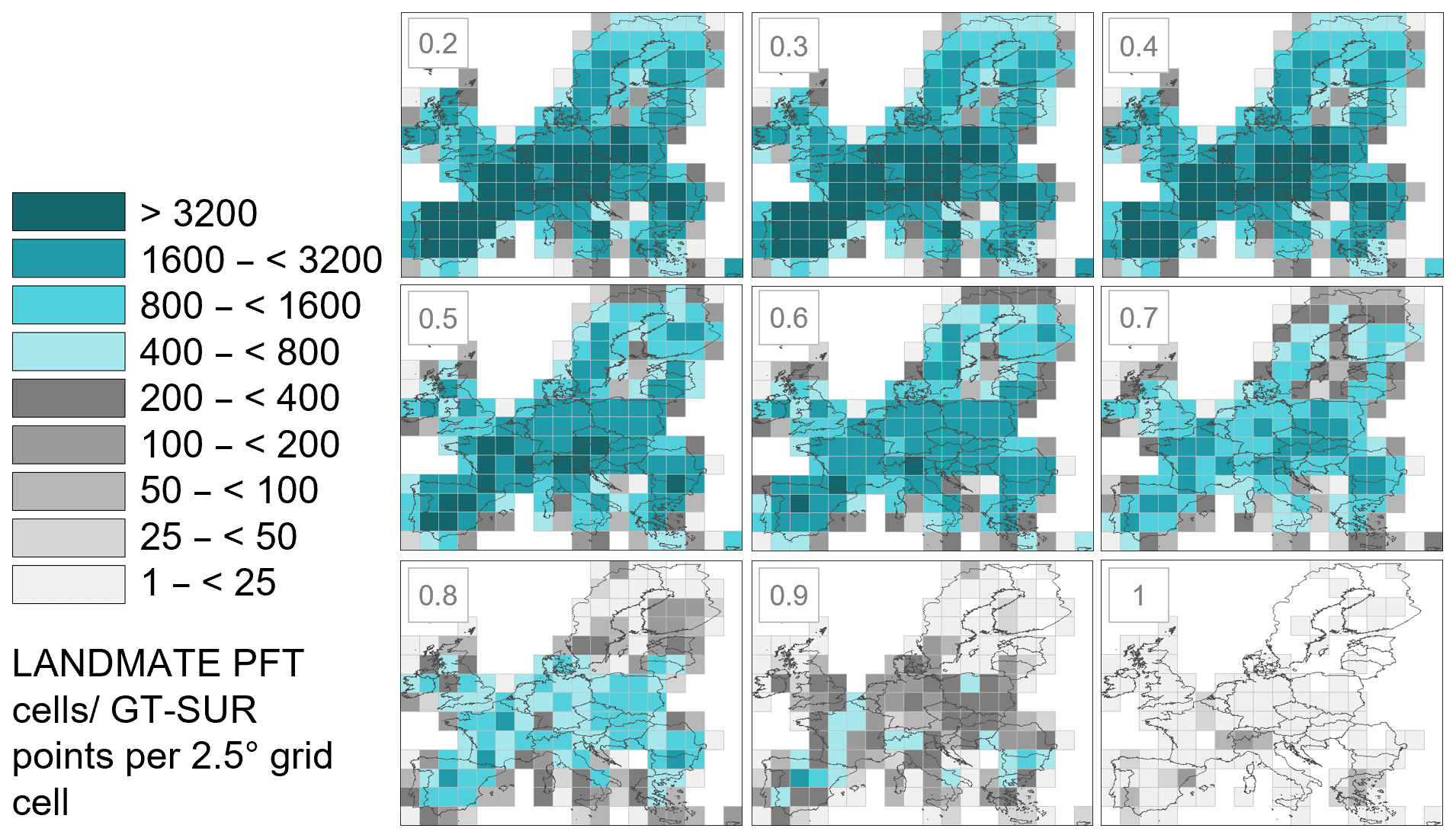
Figure 5The distribution of the LANDMATE PFT cells grouped by threshold for minimum coverage of the respective dominant LULC type over the research area in Europe. The same number of LANDMATE PFT cells falls into the groups with minimum coverages of 0.1 and 0.2. Therefore, the 0.1 group is not shown in the figure.

Figure 6Cell count (a), user's accuracy (b) and producer's accuracy (c) per LULC type of the LANDMATE PFT as a function of the threshold for minimum coverage of the respective dominant LULC type.
The spatial analysis for the six assessed LULC types for the 0.7 group is shown in Fig. 7. In order to give an overview of the spatial agreement patterns for the range of evaluable groups, the respective figures for the 0.2 and 0.5 groups are included in Appendix B (Figs. B1 and B2).

Figure 7Total count of evaluated LANDMATE PFT grid cells per 2.5∘ grid cell of the auxiliary grid as introduced in Sect. 4.1 (a–c; g–i) and producer's accuracy for the individual LULC types (d–f; j–l) for group 0.7 (the dominant LULC type occupies >70 % per LANDMATE PFT grid cell).
The urban representation in LANDMATE PFT for the 0.7 group is shown in Fig. 7a and d. Figure 6c shows that the PA for all groups is overall low and not majorly influenced by the threshold for minimum coverage. With increasing coverage of the dominant LULC type URBAN, the PA increases slightly but is still lower than 40 % for groups that include enough points to be considered representative of the research area.
A visualization of the map agreement between LANDMATE PFT and GT-SUR reveals the issue that leads to the overall low PA. Figure 8 shows four large URBAN agglomerations in different areas of Europe, where the red points represent GT-SUR urban points and the white points represent GT-SUR points representing non-urban LULC types. The grey-scaled squares represent the LANDMATE PFT URBAN fractions from zero (no coverage, white) to one (full coverage, black) within one grid cell.
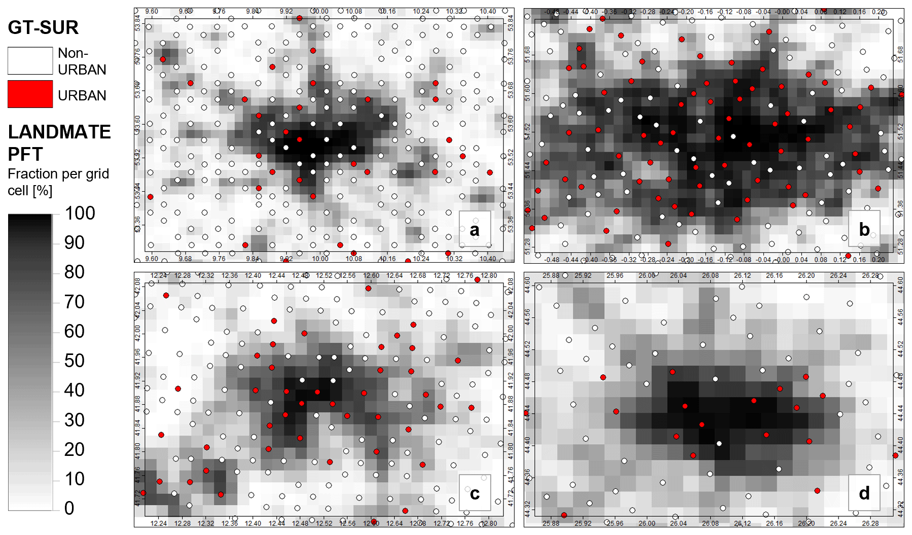
Figure 8Examples of URBAN representation in LANDMATE PFT (grey-scale grid) and GT-SUR (points). Cities shown are Hamburg (a), London (b), Rome (c) and Bucharest (d).
The LANDMATE PFT grid cells with a large urban fraction represent the respective city core of the selected example cities, while the GT-SUR points that are located within the city core are mostly not classified as URBAN. However, the GT-SUR points do not fail to represent the structure of urban areas because these areas are characterized through a heterogeneous pattern of sealed surfaces, recreational areas (e.g. parks) and different building types and density, not through a homogeneous sealed area. The LANDMATE PFT map represents this heterogeneous structure through the varying fractions of non-urban PFTs within the grid cell. However, in order to make the impact of a larger city visible in an RCM simulation, it is beneficial for LANDMATE PFT to represent a larger city with a dense core structure. Further, the URBAN fractions in LANDMATE PFT are directly adopted from the ESA-CCI LC dataset, which was thoroughly validated. Therefore, despite the low agreement with GT-SUR in the present assessment, the URBAN PFT of LANDMATE PFT 2015 is considered to be of sufficiently good quality and suitable for representing urban land cover in high-resolution (∼ 3 km) RCM simulations. Due to the aforementioned comparability issues, the UA of the LULC type URBAN is not further discussed in this assessment.
The CROPLAND representation in LANDMATE PFT shows, together with WOODLAND, the highest PA for the research area. As shown in Fig. 6c, the PA for all 10 groups is >80 %, which is to be considered very good agreement with the reference.
Figure 7b shows the distribution of CROPLAND points in GT-SUR over the research area. CROPLAND points are the second-most frequent LULC type in GT-SUR and are mainly distributed over central and southern Europe. Although the northern European grid cells show a lower count of CROPLAND points, Fig. 7e shows that the PA is still very high in these areas. The PA increases with increasing cell homogeneity (Figs. B1e and B2e). Regarding the UA for CROPLAND, LANDMATE PFT shows a strong overestimation, where ∼ 36 % of the LANDMATE PFT CROPLAND cells in the 0.7 group are actually another LULC type in the reference, where 36 % are GRASSLAND and 13 % are WOODLAND. The UA for CROPLAND increases rapidly towards the more homogeneous groups. However, the confusion with WOODLAND and GRASSLAND is non-negligible and will be discussed in Sect. 7.
For the representation of WOODLAND, the PA shows the second-highest values, with >70 % for all groups with a reasonably high cell count (groups 0.1–0.7, Fig. 6c). Similar to CROPLAND, the cell heterogeneity does not have a large impact on PA. The highest PA is reached over the northern European regions (Fig. 7f). Deficits are visible over the southern United Kingdom, parts of the Iberian Peninsula and the coastline along Belgium and the Netherlands. Further, a low PA is found for cells that have an overall small cell count in the Mediterranean (Fig. 7c).
The differences between northern and southern regions tend to increase towards the more homogeneous groups (see Figs. B1f and B2f for comparison). Agreement over the northern regions increases, while agreement over the Iberian Peninsula decreases together with a rapid decrease in the WOODLAND cell count within the corresponding grid cells. The UA for WOODLAND is noticeably higher than for all other LULC types (>70 % for the 0.2 group and increasing towards the more homogeneous groups), which emphasizes the very good quality of WOODLAND representation in LANDMATE PFT. The most confusion is found with LULC type GRASSLAND and the OTHER LULC types (not investigated in this assessment). Altogether, the UA of ∼ 85 % for group 0.7 is interpreted as a very good representation of the LULC type WOODLAND within LANDMATE PFT 2015.
The coverage of cells with the dominant LULC type GRASSLAND is well distributed except for the northern European regions (Fig. 7h). The PA for LANDMATE PFT GRASSLAND according to Fig. 7k is very high in the United Kingdom and in some regions of central Europe. For the remaining regions of the research area, the PA for GRASSLAND is considerably low. This PA pattern remains similar throughout the range of evaluable groups (Figs. B1k and B2k), with an average of 31 %–37 %.
The main reason for this low accuracy of LANDMATE PFT regarding GRASSLAND can be found by looking at the results of the LULC types CROPLAND and WOODLAND. The UAs of CROPLAND and WOODLAND reveal that ∼ 36 % of the LANDMATE PFT CROPLAND cells actually represent GRASSLAND in the reference, which adds up to over almost 55 % of the total GT-SUR GRASSLAND points. Another reason is found in the dataset structure of LANDMATE PFT. A considerable amount of GRASSLAND is not part of the assessment because GRASSLAND does not make up the dominant but rather the second-most dominant PFT in ∼ 45 % of all LANDMATE PFT grid cells. Therefore, the seemingly weak GRASSLAND representation in LANDMATE PFT rather shows a weakness of the present assessment that is caused by the different dataset structures.
The PA for SHRUBLAND and BARE AREAS is the lowest of all assessed LULC types, with <20 % for all groups of both LULC types, respectively (Fig. 6c). The low overall cell count of both LULC types might be one reason for the low PA. However, looking at the distribution of the SHRUBLAND and BARE AREA points in Fig. 7g and i, LANDMATE PFT is not able to capture the LULC types even in grid cells with a relatively high cell count. The GT-SUR includes ∼ 27 000 SHRUBLAND points, while LANDMATE PFT includes only ∼ 19 000 cells where SHRUBLAND is the dominant LULC type. Therefore, one reason for the poor SHRUBLAND representation lies within the base map (ESA-CCI LC) used for the creation of LANDMATE PFT, where the known low count of SHRUBLAND proportions was inherited by LANDMATE PFT. It must be noted that a large proportion of SHRUBLAND in ESA-CCI LC is part of the mixed LC classes, such as Shrubland/Cropland or Shrubland/Forest. The known deficit was partly compensated by the translation into the PFTs, where SHRUBLAND proportions were added to the total as proportions of the mixed ESA-CCI LC classes. Further, SHRUBLAND makes up the second-most dominant PFT in ∼ 20 % of the total LANDMATE PFT grid cells in the assessment. Just like for GRASSLAND, these SHRUBLAND proportions cannot be addressed sufficiently within the present assessment.
The overall BARE AREAS cell count in LANDMATE PFT in the 0.7 group is only about 28 % of the actual BARE AREA points in GT-SUR. Further, within the 0.7 group, over 64 % of the GT-SUR BARE AREAS points are identified as CROPLAND, while only ∼ 17 % (<1000 points for the 0.7 group) of the GT-SUR BARE AREAS are actually identified by LANDMATE PFT, with the highest PA in the Alps, northern Great Britain, and northern Scandinavia (Fig. 7l). However, due to the comparably low cell count, the spatial assessment is rather not reliable. Just like for SHRUBLAND, the homogeneity of LANDMATE PFT cells does not have a large impact on the PA. UA is higher than PA, with ∼ 43 % for group 0.2 and increasing towards more homogeneous groups (over 60 % for group 0.7). However, considering the rapidly decreasing cell count for the more homogeneous groups, the accuracy measures are becoming even less representative of the BARE AREA representation in LANDMATE PFT. Nevertheless, the BARE AREA representation in LANDMATE PFT is further discussed in Sect. 7.
5.1 Comparison to ESA POULTER PFT validation results
In order to compare the LANDMATE PFT map quality to the ESA POULTER PFT map quality, the validation workflow presented in this paper is also applied to the latter for the year 2015. The PA differences of LANDMATE PFT and ESA POULTER PFT are shown in Fig. 9. The spatial PA differences vary between the assessed LULC types and groups. For URBAN, the differences are negligible. Since the ESA-CCI LC URBAN proportions are directly adopted in both PFT translations, this result was expected. The small differences in some grid cells of the map might result from the changes in the CWP within the LANDMATE PFT workflow that cause other LULC types to be of dominant coverage and therefore change the total cell counts per LULC type in the aggregation. LANDMATE PFT represents CROPLAND slightly worse than ESA POULTER PFT according to the differences seen on the maps. The difference is mainly caused by the translation of the “cropland tree or shrub cover” class of ESA CCI LC, which is dominant in the Mediterranean region. Within the LANDMATE PFT translation, the LC class is translated into 70 % shrubs and 30 % cropland according to Li et al. (2018). Using this translation, the Mediterranean cropland properties, where the cultivation of lemons or olives makes up a large proportion of the total agricultural landscape, are better represented. These types of cultivation grow in short- to medium-height trees with the properties of shrubs rather than cropland. Therefore, a considerable number of dominant cropland cells are changed into dominant shrubland cells within the comparison to GT-SUR, which is reflected in the accuracy numbers in Fig. 9. The threshold for minimum coverage does not have considerable influence on the CROPLAND representation, except for northern Europe, where the highest minimum coverage threshold (0.7) shows the lowest PA for cropland. In contrast, the LANDMATE PFT WOODLAND representation is most improved for the highest minimum threshold (0.7) in comparison to the ESA POULTER PFTs. A similar result is found for the GRASSLAND representation. It is noticeable that the signal changes for the BARE AREAS representation. For the group with a minimum coverage of 0.2, ESA POULTER PFT shows the better BARE AREAS representation, while for the 0.7 group, LANDMATE PFT shows the better quality.
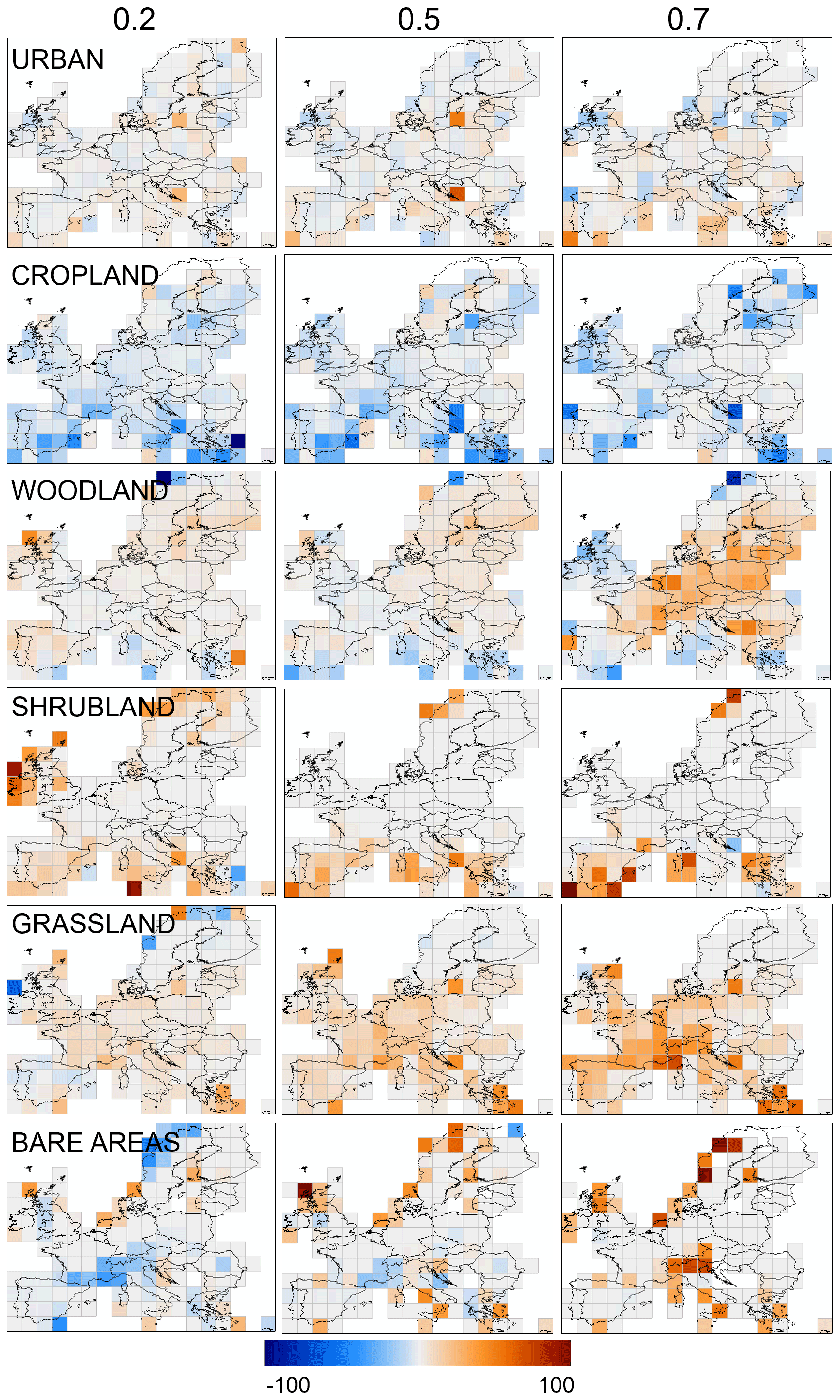
Figure 9Comparison between the PA for LANDMATE PFT and ESA PFT. The plots show the differences between the PA, where the positive values mean a higher PA of LANDMATE PFT and the negative values a higher PA of ESA POULTER PFT. The differences were calculated per 2.5∘ grid cell of the auxiliary grid as introduced in Sect. 4.1 for each LULC type of the 0.2 group (left column), the 0.5 group (middle column) and the 0.7 group (right column).
The LANDMATE PFT dataset for Europe 2015 is published with the Long Term Archiving Service (LTA) for large research datasets, which are relevant for climate or Earth system research, of the German Climate Computing Service (DKRZ). Like the World Data Center for Climate (WDCC), the DKRZ LTA is accredited as a regular member of the World Data System. The LANDMATE PFT dataset for Europe 2015 is available within the LANDMATE project data at http://doi.org/10.26050/WDCC/LM_PFT_LandCov_EUR2015_v1.0 (Reinhart et al., 2021b). Within the LANDMATE project, brief documentation summarizes the technical information corresponding to LANDMATE PFT.
The present work introduces the preparation of the LANDMATE PFT map 2015 for the European continent based on high-resolution LULC datasets and climate data. The LANDMATE PFT map for 2015 Version 1.0 is prepared in order to provide realistic, high-resolution LULC representation for RCMs. The dataset includes LULC information from different, validated sources as well as regional climate information through involvement of the HLZs. A cross-walking procedure (CWP) is developed to translate the original LULC classes into PFTs. The various mixed LULC classes included in the base map ESA-CCI LC are difficult to resolve within RCMs, which is taken into account by ESA by providing a default CWT for the translation of the LC classes into PFTs within the dedicated user tool. The revised and improved CWTs of the present approach include high-resolution climate data in the translation. The involvement of climate data allows customized translation of LULC classes for individual regions in addition to the disaggregation of LULC classes into PFT fractions. The 16 LANDMATE PFTs are selected to provide simple transferability to various RCM families in order to be able to conduct coordinated RCM experiments where the implementation of a common, high-quality LULC map provides minimum uncertainty for a multi-model ensemble.
The accuracy assessment of LANDMATE PFT is conducted in the form of a comparison to the ground truth dataset LUCAS land use and land cover survey (GT-SUR). In order to account for the different structure of the reference GT-SUR and the assessed LANDMATE PFT map and, further, the fractional structure of the LANDMATE PFT grid cells, the grid cells are grouped by a threshold for minimum coverage of the dominant LULC type. All groups are analysed regarding agreement with the reference (i.e. GT-SUR). In order to investigate regional differences in accuracy measures, a spatial analysis supported by an auxiliary grid over the research area is done. The quality of the LANDMATE PFT map is assessed using the overall accuracy (OA) and the producer's and user's accuracy (PA and UA) for the individual LULC types. The additional comparison to the generic ESA POULTER PFT map (ESA POULTER PFT) should give information on the regional improvement of LULC type representation in LANDMATE PFT. Overall, the validation serves as recommendation and uncertainty information for regional climate modellers who use LANDMATE PFT or the time series LUCAS LUC (Hoffmann et al., 2021), which is based on LANDMATE PFT, in RCMs.
Within the accuracy assessment, the OA does not change considerably between the evaluable groups of the respective LULC types, which shows that the dataset structure has no noticeable impact on that accuracy measure. The highest PA is found for CROPLAND and WOODLAND, which are the dominant LULC types in the research area. The lowest PA is found for SHRUBLAND and BARE AREAS, which are also the LULC types with the lowest overall cell count. The UA is found to be highest for WOODLAND, followed by CROPLAND, GRASSLAND and BARE AREAS. Both accuracy measures, PA and UA, are influenced by grid cell heterogeneity of the dominant LULC type within a grid cell. The difference between the groups for UA is 10 % to 20 % per group, while the difference for PA is noticeable but considerably lower, which means that the applied threshold range has a higher influence on the former.
The URBAN representation in LANDMATE PFT represents a special case in the present assessment due to the heterogeneous structure of urban areas. Both datasets, GT-SUR and LANDMATE PFT, are able to represent the LULC type URBAN very well for their respective purposes. Nevertheless, the PA for URBAN reflects the limitations of the present assessment method. The fine-scale point data of GT-SUR represent the patchwork structure of recreational areas, building blocks, and other urban elements at the locations of the respective points, while LANDMATE PFT represents the urban area as an agglomeration of grid cells with URBAN as the dominant LULC type. Therefore, and despite the accuracy assessment results for the LULC type URBAN, the LANDMATE PFT dataset can be recommended for use in RCMs that resolve urban features over the European continent.
A limitation of LANDMATE PFT is the overestimation of CROPLAND at the expense of GRASSLAND and WOODLAND and the overestimation of WOODLAND at the expense of mostly GRASSLAND. This overestimation has a minor impact on the overall WOODLAND and CROPLAND representation but a major impact on the representation of GRASSLAND in LANDMATE PFT. The representation of GRASSLAND is comparably low for the aforementioned reasons. Further, the LULC types with the lowest point counts SHRUBLAND and BARE AREAS are not well represented, which happens due to the low overall sample size but also due to the overall too low representation in LANDMATE PFT, which is partly inherited from the base map ESA-CCI LC. The representation of these LULC types needs to be considered when using LANDMATE PFT in RCM simulations using the supporting maps in Figs. 7, B1 and B2. Nevertheless, the representation of SHRUBLAND and BARE AREAS is improved in some regions compared to ESA POULTER PFT.
Another limitation is the distinction between C3 and C4 grass and the missing irrigated cropland fractions. The distinction between C3 and C4 grass is made through the use of an additional product and is not based on the HLZ approach. Further, the grass fractions are not evaluated separately due to the missing C3/C4 grass information in GT-SUR. The suggested that C3/C4 grass distribution in LANDMATE PFT relies on a product that is dedicated to the C3/C4 grass representation and employed by climate modellers. However, the use of the external product holds additional uncertainties within LANDMATE PFT that cannot be quantified with the present assessment method. The main focus of LANDMATE PFT Version 1.0 is on the representation of biophysical properties of LULC types within RCMs. While C3 and C4 grasses differ in their biophysical properties, which is the reason to include them as separate PFTs, the main impacts can be expected for biogeochemical processes. Hence, for the further improvement of LANDMATE PFT and for the use of this dataset for the modelling of the carbon cycle, it is advisable to put additional effort into the implementation and evaluation of C3/C4 grass fractions.
Regarding the irrigated cropland fractions, we aimed to proceed the same way as for the C3/C4 grass fractions – to rely on an external product because the land cover category provided by ESA-CCI LC does not cover the full extent of irrigated land use. Unlike for C3/C4 grass, where one particular high-quality product is available, the multiple products that were considered are of different structure, resolution, and acquisition date and show considerable differences in irrigated cropland proportions. Also, the ESA-CCI LC class “cropland irrigated” that could have been directly adopted from the initial LC dataset shows considerable differences to the other state-of-the-art products. Since irrigation is a land management practice that is shown to have large biophysical impacts on regional climate and that therefore is of importance to the RCM community, we prepared the dataset to easily implement irrigated cropland using additional datasets. For instance, in the time series LUCAS LUC, which is based on the LANDMATE PFT dataset, the annually varying irrigated cropland fractions are taken from the LUH2 dataset in order to be consistent for the past and future time steps.
Further improvements could be made with respect to the distinction of tree PFTs. Currently, six tree PFTs are considered in LANDMATE PFT following Wilhelm et al. (2014), with two tropical broadleaf tree PFTs, two broadleaf temperate tree PFTs, and two coniferous tree PFTs. The CWP employed in this study could be further refined to include a separation between temperate and boreal tree PFTs, which would involve a careful extension of the individual CWTs.
The quality of the representation of LULC types in LANDMATE PFT is assessed through the comparison to ground truth data. The structural differences of the datasets, where gridded data are compared to point data, is a major weakness of this assessment. Although the fractional structure does not have a major influence on the OA, the LULC type-wise PA and even more the UA are affected.
The present assessment takes into account the dominant LULC type per grid cell of LANDMATE PFT. Depending on the proportion of this LULC type, the second- or third-most represented LULC type can occupy a considerable area of the respective grid cell. Therefore, a follow-up assessment where these LULC type proportions are also considered and compared to the ground truth is needed in order to investigate whether the PA of the less dominant LULC types GRASSLAND, SHRUBLAND and BARE AREAS is increased. The use of additional LULC data specialized in one LULC type would be a useful step to validate the quality of GRASSLAND, SHRUBLAND and BARE AREAS representation in LANDMATE PFT 2015.
The results show that the LANDMATE PFT map is able to represent LULC over large parts of Europe with sufficient quality. Especially the dominant LULC types are represented overall well, which is highly beneficial for RCM experiments that require realistic, high-resolution LULC representation. Nevertheless, there are uncertainties found for the less represented LULC types. Regarding the presence of less represented LULC types, we did a qualitative assessment where we checked certain locations of interest with other available datasets (e.g. CORINE Land Cover, Google Earth images) supporting the development process of the CWTs. The additional cross-checking did improve the quality of the final LANDMATE PFT map. However, it was not done with a pre-defined workflow or protocol. Hence, we suggest developing a strategic and quantifiable sampling protocol for the qualitative assessment as an additional step within the map production workflow. This could further improve the CWTs and subsequently the PFT product. When using LANDMATE PFT in an RCM, it is crucial to consider these uncertainties when interpreting simulation results. Especially the spatial distribution of uncertainties in LANDMATE PFT needs to be considered when comparing simulation results to observations because the input parameters in the employed land surface schemes are influenced by the individual LULC, which subsequently considerably impacts lower-atmosphere processes, such as the intensity of heat and moisture exchange. Thus, by carefully considering the issue of uncertainty introduced by the LULC input, incorrect conclusions about RCM model performance and about small-scale interconnections can be reduced (Ge et al., 2007; Sertel et al., 2010; Santos-Alamillos et al., 2015; Reinhart et al., 2021a).
Besides the quality of the LULC product, the implementation process of each individual RCM is crucial for the realistic representation of LULC in regional climate model experiments. When translating a LULC product into the model-specific LULC classes and structure, modifications are done that can change the map characteristics. When the LANDMATE PFT product is used in an RCM that only uses the dominant LULC fraction per grid cell, the overall LULC proportions can change. The same applies when LANDMATE PFT is used in a model with limited fractions per grid cell or a different classification system. The present assessment gives a guideline on the quality of LANDMATE PFT (Version 1.0) when used unaltered. Through the involvement of the ground truth data, regional deficits of LANDMATE PFT are presented that can be compensated for during the implementation process in the individual RCM or RCM family.
The findings of the present assessment support the identification of uncertainties within the LANDMATE PFT map for Europe. Nevertheless, user feedback is crucial for the future overall improvement of LANDMATE PFT. The RCM community within the WCRP (World Climate Research Programme) FPS LUCAS is already participating in the feedback process where implementation of LANDMATE PFT and the LUCAS LUC time series in different RCMs is comprehensively documented. The future work on LANDMATE PFT also includes the extension of the dataset to other CORDEX regions. Although the dataset is based on various globally available datasets and therefore can be created globally, the introduced quality assessment method must be performed for each region individually, preferably using region-specific expert knowledge. Further, the assessment should be expanded in order to include the second- or third-most represented LULC type per grid cell to possibly achieve more accurate quality information about LANDMATE PFT.
Table A1Cross-walking table for ESA-CCI LC class 10 – Cropland, rainfed – and LC class 11 – Cropland, herbaceous cover. For LC classes 10 and 11, no HLZs were assigned.

Table A2Cross-walking table for ESA-CCI LC class 12 – Cropland, tree or shrub cover. For LC class 12, no HLZs were assigned.

Table A3Cross-walking table for ESA-CCI LC class 20 – Cropland, irrigated or post flooding. For LC class 20, no HLZs were assigned.

Table A4Cross-walking table for ESA-CCI LC class 30 – Mosaic cropland (>50 %)/natural vegetation (tree, shrub, herbaceous cover) (<50 %).
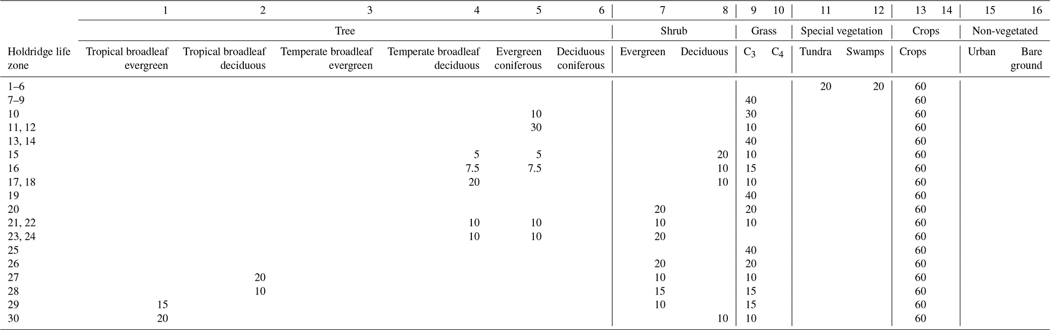
Table A5Cross-walking table for ESA-CCI LC class 40 – Mosaic natural vegetation (tree, shrub, herbaceous cover) (>50 %)/cropland (<50 %).
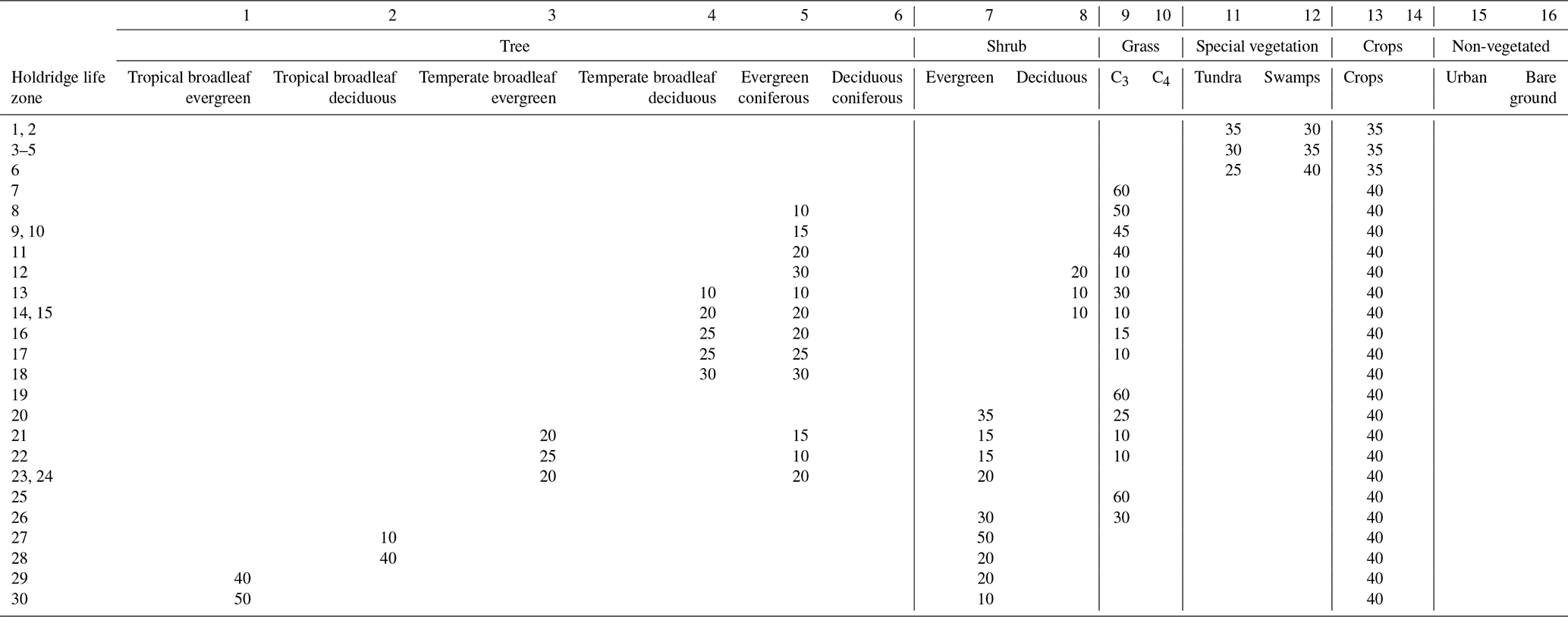
Table A6Cross-walking table for ESA-CCI LC class 50 – Tree cover, broadleaved, evergreen, closed to open (>15 %).
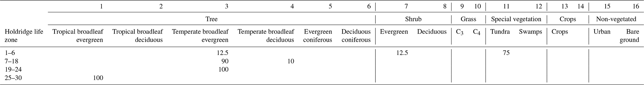
Table A7Cross-walking table for ESA-CCI LC class 60 – Tree cover, broadleaved, deciduous, closed to open (>15 %).

Table A8Cross-walking table for ESA-CCI LC class 61 – Tree cover, broadleaved, deciduous, closed (>40 %).
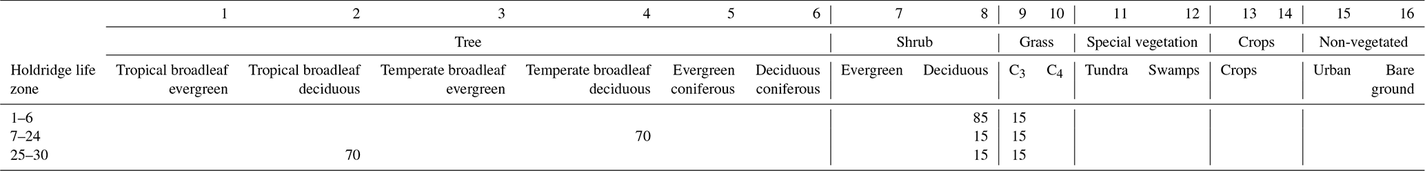
Table A9Cross-walking table for ESA-CCI LC class 62 – Tree cover, broadleaved, deciduous, open (15 %–40 %).

Table A10Cross-walking table for ESA-CCI LC class 70 – Tree cover, needleleaved, evergreen, closed to open (>15 %) – and LC class 71 – Tree cover, needleleaved, evergreen, closed (>40 %).

Table A11Cross-walking table for ESA-CCI LC class 72 – Open (15 %–40 %) needleleaved deciduous or evergreen forest (>5 m).
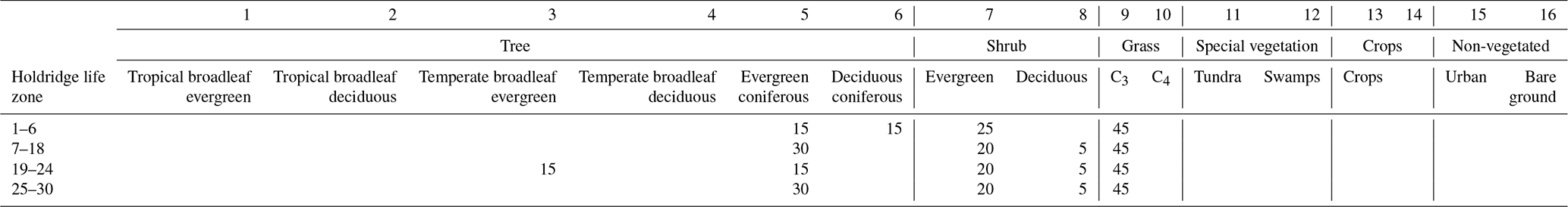
Table A12Cross-walking table for ESA-CCI LC class 80 – Tree cover, needleleaved, deciduous, closed to open (>15 %).

Table A13Cross-walking table for ESA-CCI LC class 81 – Treecover, needleleaved, deciduous, closed (>40 %).

Table A14Cross-walking table for ESA-CCI LC class 82 – Tree cover, needleleaved, deciduous, open (15 %–40 %).

Table A15Cross-walking table for ESA-CCI LC class 90 – Tree cover, mixed leaf type (broadleaved and needleleaved).
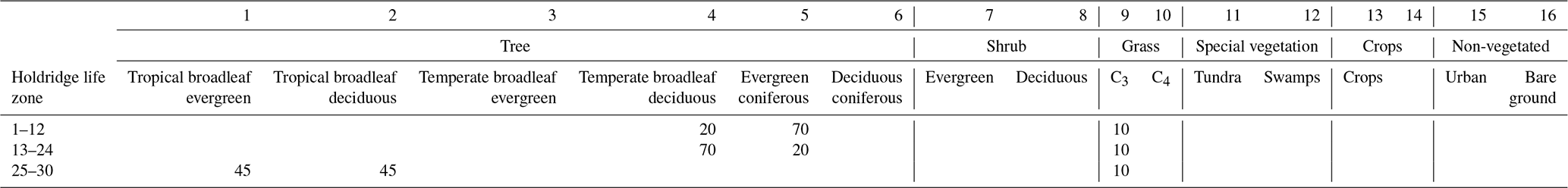
Table A16Cross-walking table for ESA-CCI LC class 100 – Mosaic tree and shrub (>50 %)/herbaceous cover (<50 %).
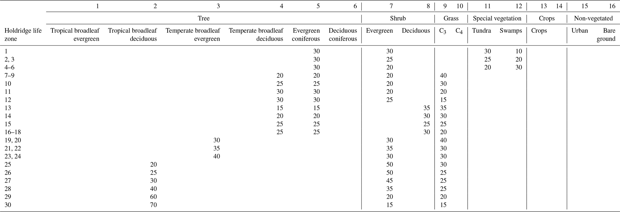
Table A17Cross-walking table for ESA-CCI LC class 110 – Mosaic herbaceous cover (>50 %)/tree and shrub (<50 %).
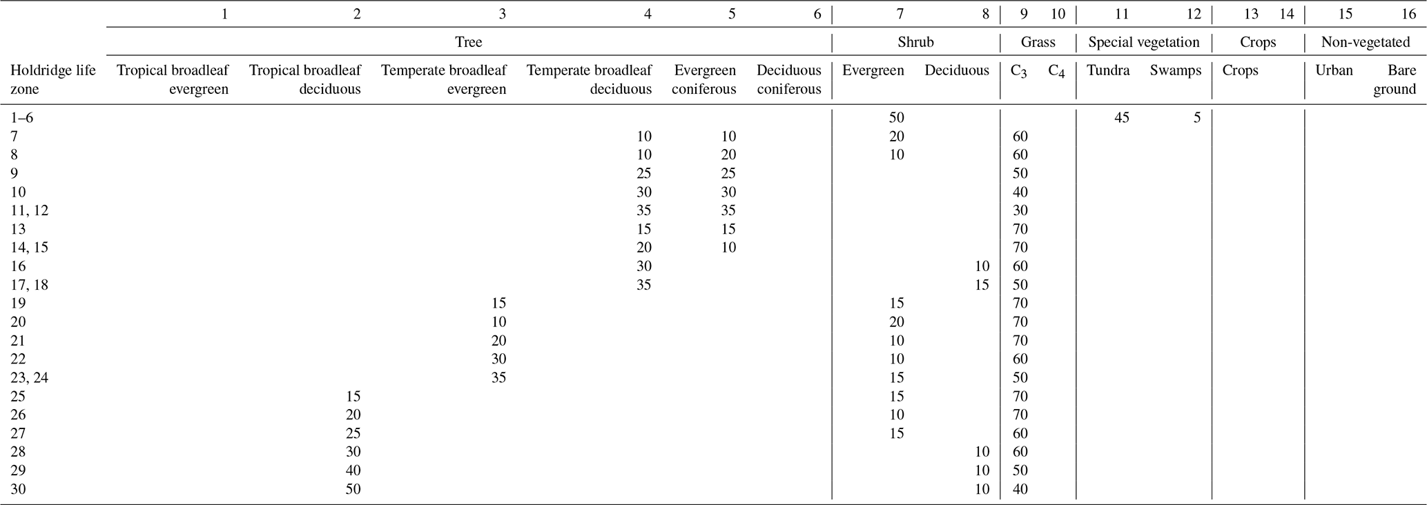
Table A18Cross-walking table for ESA-CCI LC class 120 – Shrubland.
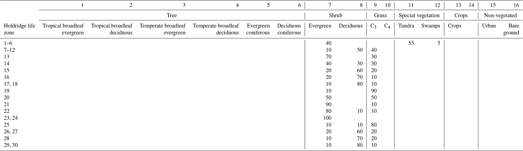
Table A19Cross-walking table for ESA-CCI LC class 121 – Evergreen shrubland – and LC class 122 – Deciduous shrubland.

Table A20Cross-walking table for ESA-CCI LC class 122 – Evergreen shrubland – and LC class 122 – Deciduous shrubland.
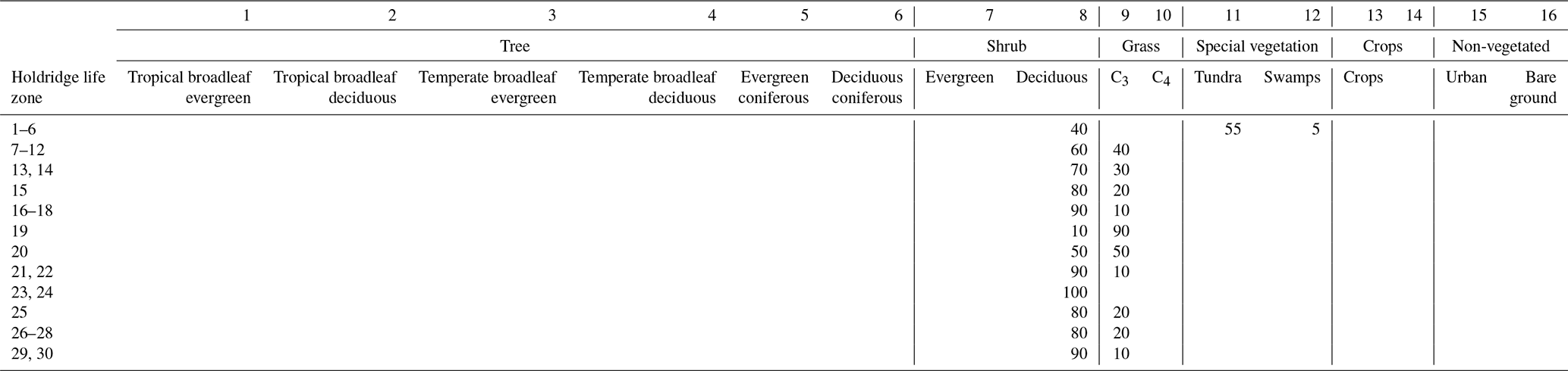
Table A21Cross-walking table for ESA-CCI LC class 130 – Grassland.
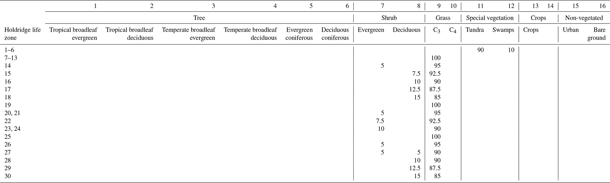
Table A22Cross-walking table for ESA-CCI LC class 140 – Lichens and mosses.
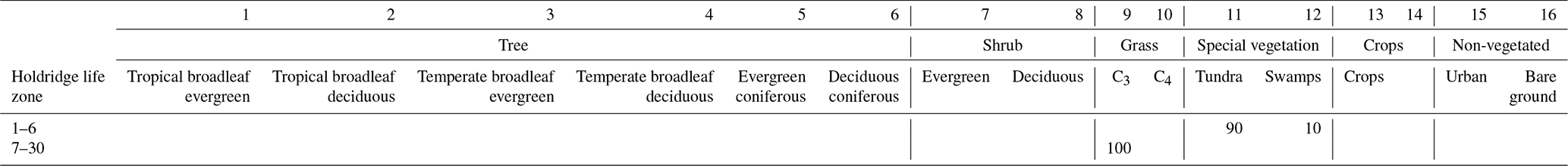
Table A23Cross-walking table for ESA-CCI LC class 150 – Sparse vegetation (tree, shrub, herbaceous cover) (<15 %).

Table A24Cross-walking table for ESA-CCI LC class 151 – Sparse tree (<15 %).
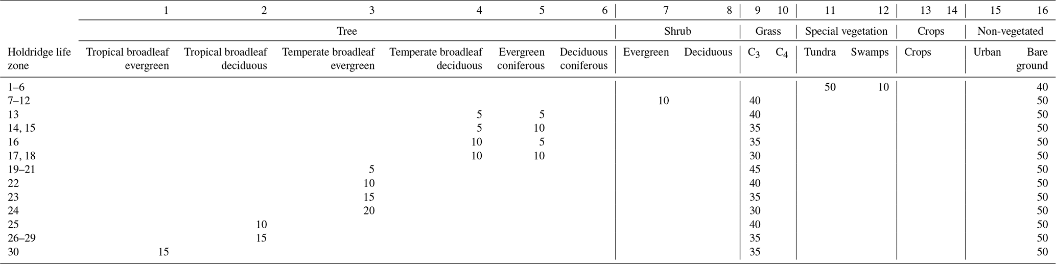
Table A25Cross-walking table for ESA-CCI LC class 152 – Sparse shrub (<15 %).
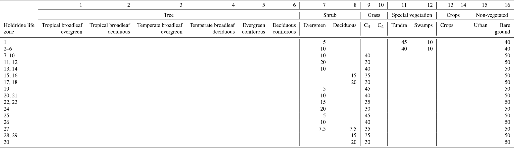
Table A26Cross-walking table for ESA-CCI LC class 153 – Sparse herbaceous cover (<15 %).
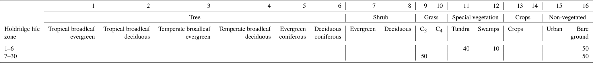
Table A27Cross-walking table for ESA-CCI LC class 160 – Tree cover, flooded, fresh or brackish water.
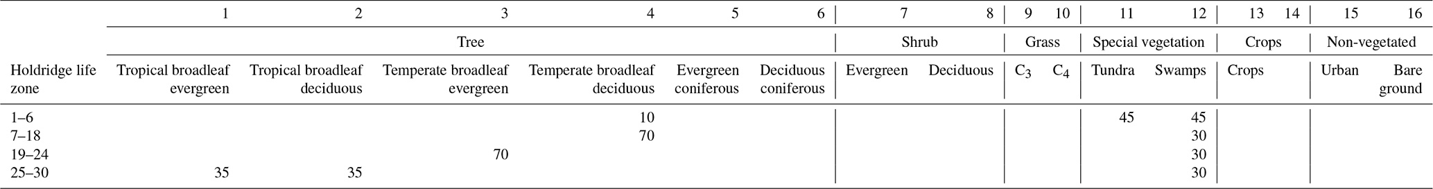
Table A28Cross-walking table for ESA-CCI LC class 170 – Tree cover, flooded, saline water.
Table A29Cross-walking table for ESA-CCI LC class 180 – Shrub or herbaceous cover, flooded, fresh/saline/brackish water.
Table A30Cross-walking table for ESA-CCI LC class 190 – Urban.

Table A31Cross-walking table for ESA-CCI LC class 200 – Bare areas – LC class 201 – Consolidated bare areas – and LC class 202 – Unconsolidated bare areas.


Figure B1Total count of evaluated LANDMATE PFT grid cells per 2.5∘ grid cell of the auxiliary grid as introduced in Sect. 4.1 (a–c; g–i) and producer's accuracy for the individual LULC types (d–f; j–l) for group 0.2 (the dominant LULC type occupies >20 % per LANDMATE PFT grid cell).

Figure B2Total count of evaluated LANDMATE PFT grid cells per 2.5∘ grid cell of the auxiliary grid as introduced in Sect. 4.1 (a–c; g–i) and producer's accuracy for the individual LULC types (d–f; j–l) for group 0.5 (the dominant LULC type occupies >50 % per LANDMATE PFT grid cell).
Table B1Confusion matrix for LANDMATE PFT group 0.1 – the dominant LULC type occupies a minimum of 10 % of a LANDMATE PFT grid cell.
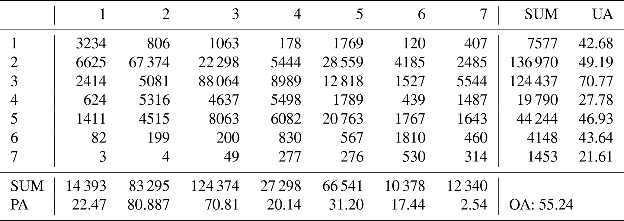
Table B2Confusion matrix for LANDMATE PFT group 0.2 – the dominant LULC type occupies a minimum of 20 % of a LANDMATE PFT grid cell.
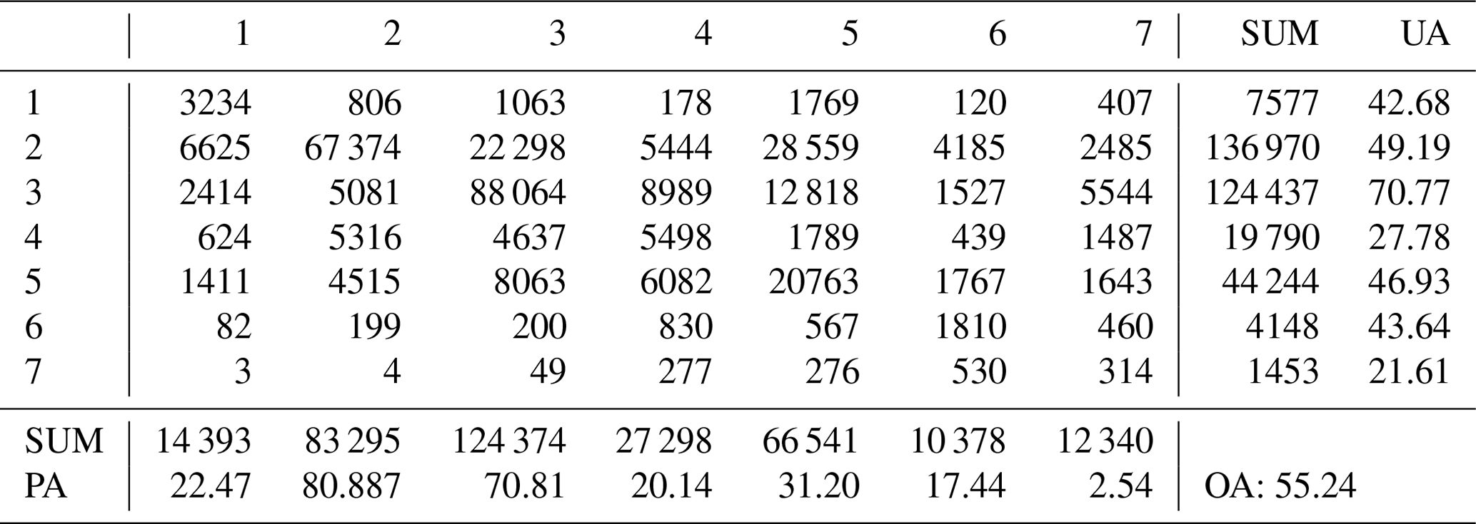
Table B3Confusion matrix for LANDMATE PFT group 0.3 – the dominant LULC type occupies a minimum of 30 % of a LANDMATE PFT grid cell.
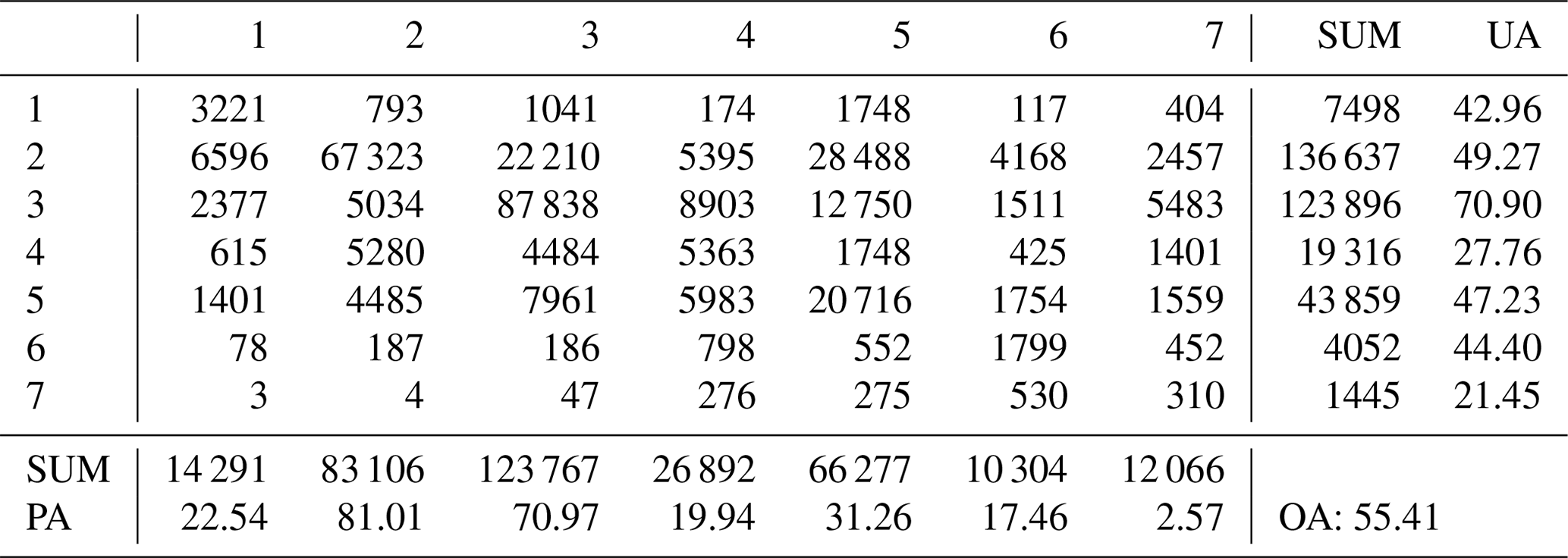
Table B4Confusion matrix for LANDMATE PFT group 0.4 – the dominant LULC type occupies a minimum of 40 % of a LANDMATE PFT grid cell.
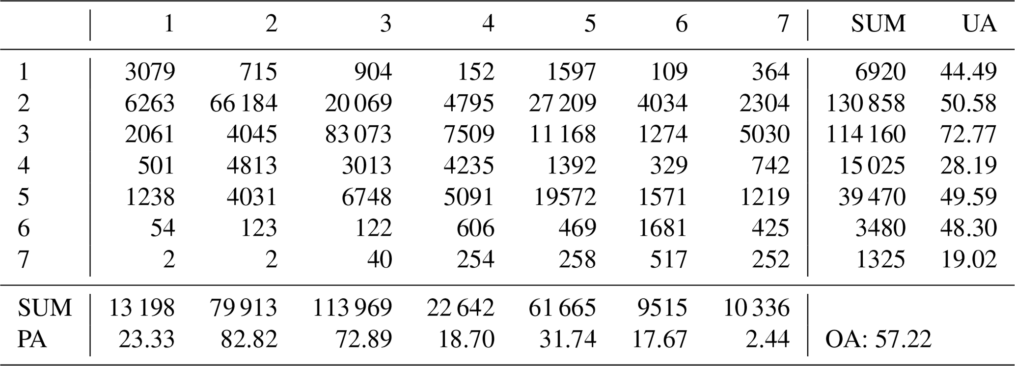
Table B5Confusion matrix for LANDMATE PFT group 0.5 – the dominant LULC type occupies a minimum of 50 % of a LANDMATE PFT grid cell.
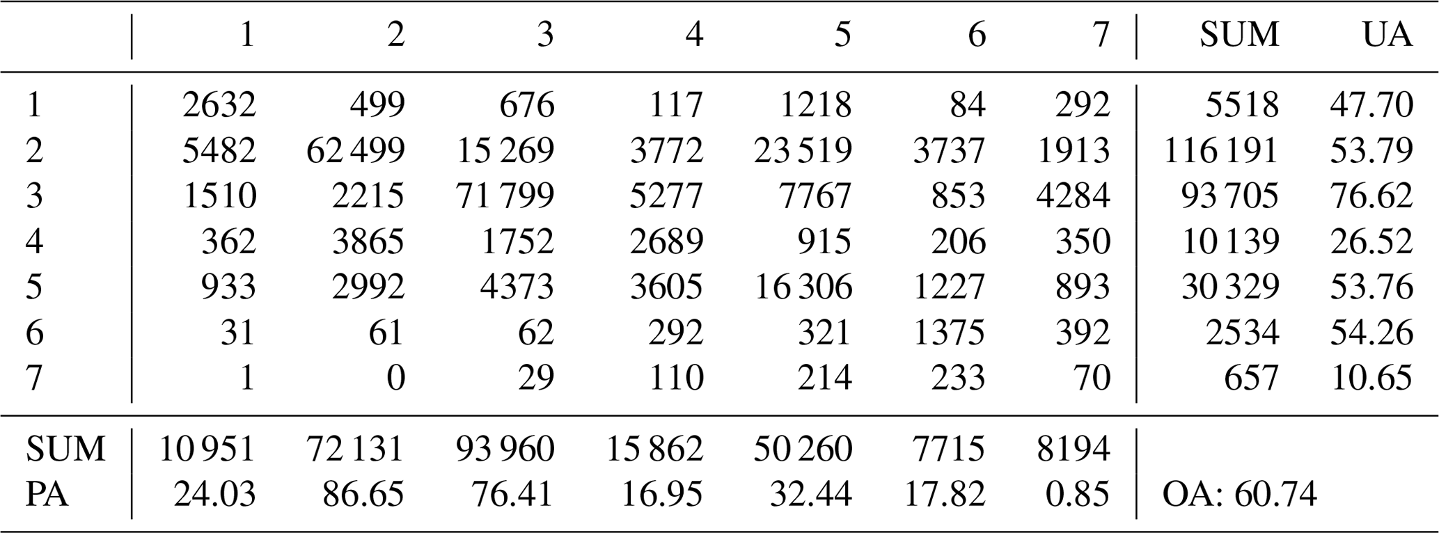
Table B6Confusion matrix for LANDMATE PFT group 0.6 – the dominant LULC type occupies a minimum of 60 % of a LANDMATE PFT grid cell.
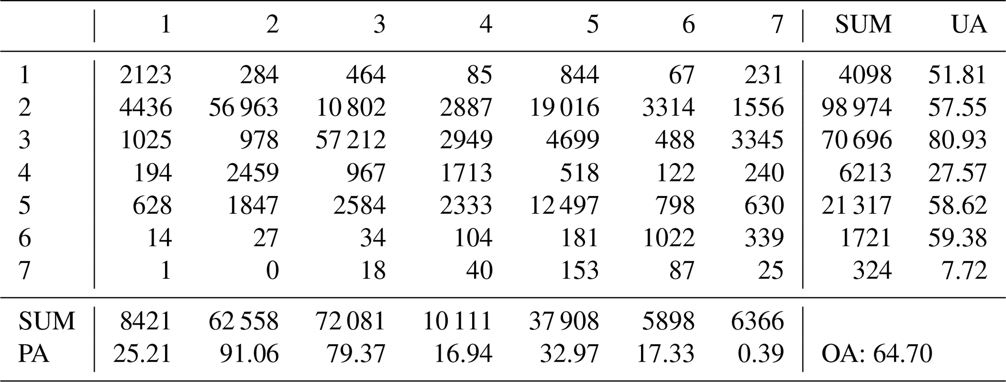
Table B7Confusion matrix for LANDMATE PFT group 0.7 – the dominant LULC type occupies a minimum of 70 % of a LANDMATE PFT grid cell.
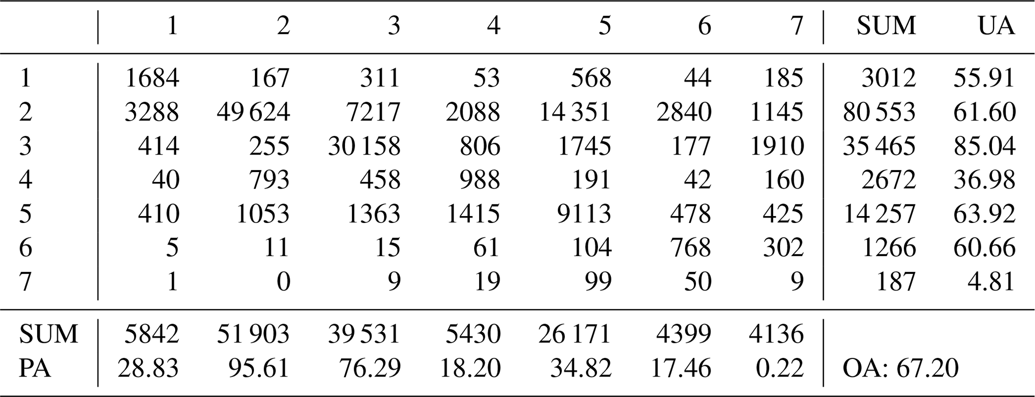
Table B8Confusion matrix for LANDMATE PFT group 0.8 – the dominant LULC type occupies a minimum of 80 % of a LANDMATE PFT grid cell.
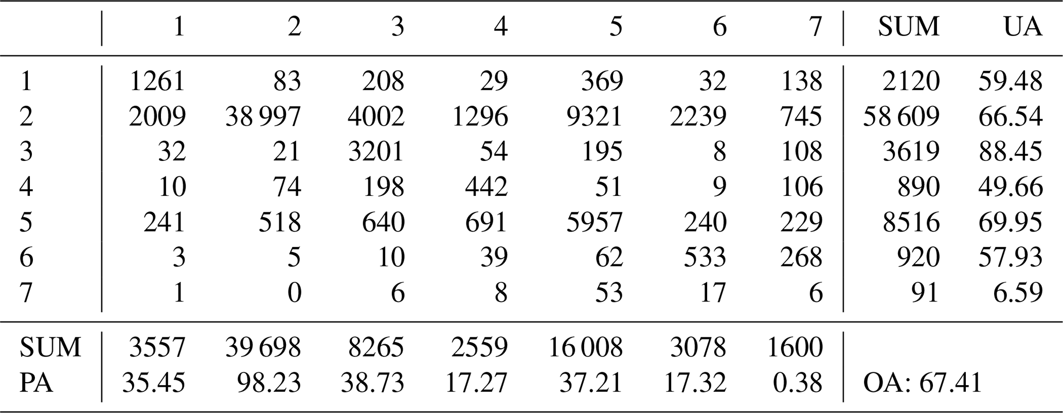
Table B9Confusion matrix for LANDMATE PFT group 0.9 – the dominant LULC type occupies a minimum of 90 % of a LANDMATE PFT grid cell.
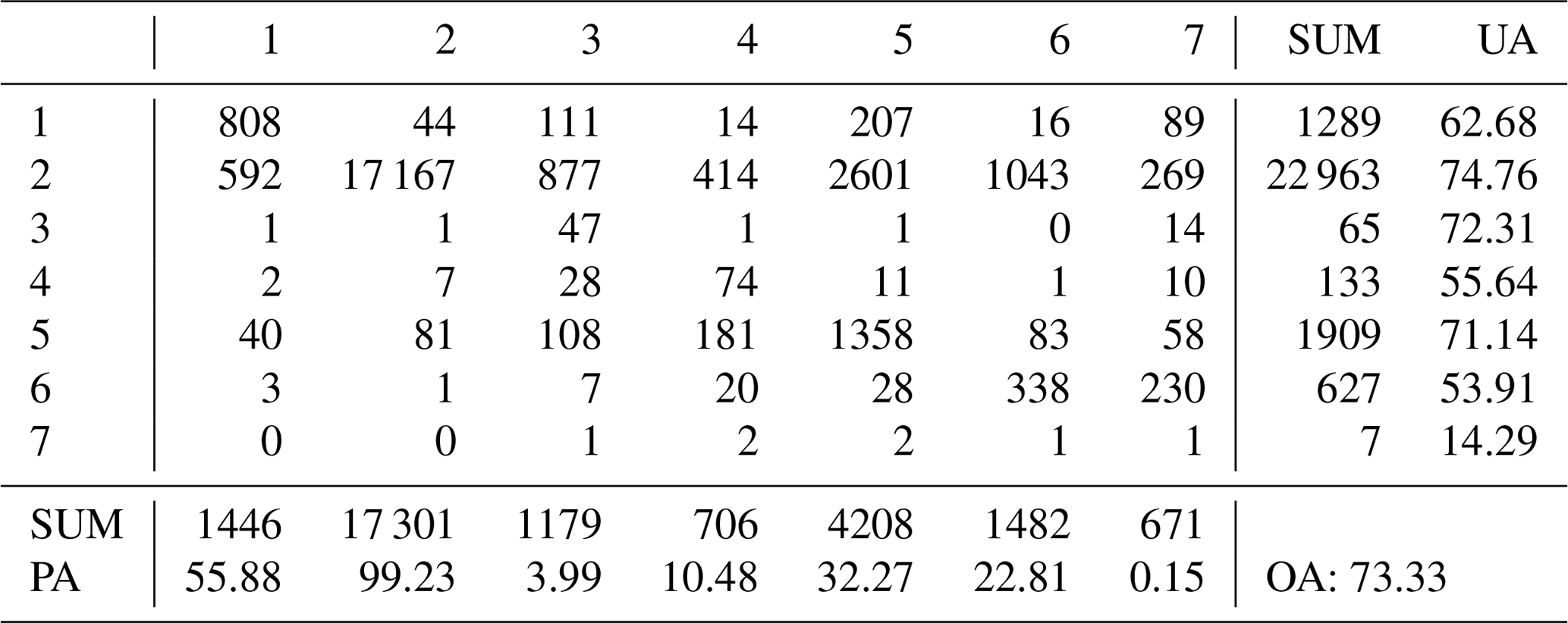
Table B10Confusion matrix for LANDMATE PFT group 1.0 – the dominant LULC type occupies 100 % of a LANDMATE PFT grid cell.
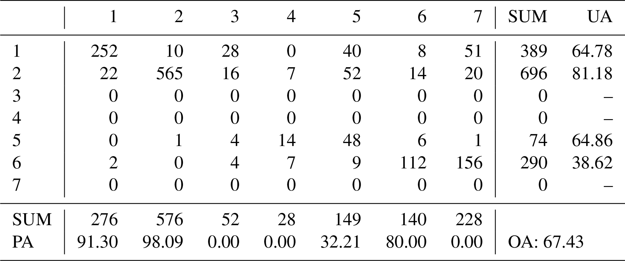
VR conceptualized the paper outline and objective with the support of DR, PH and JB. VR and PH developed the cross-walking procedure and the corresponding cross-walking tables. PH developed the required translation software for the cross-walking procedure. VR developed the accuracy assessment design for the LANDMATE PFT map, supported by BB. VR conducted the accuracy assessment and the visualization of results. VR wrote the original draft of the paper, VR, PH, DR, JB, and BB reviewed and edited the draft, and VR wrote the final paper.
The contact author has declared that neither they nor their co-authors have any competing interests.
Publisher’s note: Copernicus Publications remains neutral with regard to jurisdictional claims in published maps and institutional affiliations.
We are grateful for the support of LUCAS by WCRP-CORDEX as a Flagship Pilot Study. We are grateful for the E-OBS dataset from EU-FP6 project UERRA (http://www.uerra.eu, last access: 4 April 2022), the Copernicus Climate Change Service, and the data providers in the ECA&D project (https://www.ecad.eu, last access: 4 April 2022). We thank the European Space Agency (ESA) for making the land cover products publicly available. Special thanks go to the FPS LUCAS partners for providing useful comments in order to improve the dataset.
This work was financed within the framework of the Helmholtz Institute for Climate Service Science (HICSS), a cooperation between the Climate Service Center Germany (GERICS) and Universität Hamburg, Germany, and conducted as part of the LANDMATE (Modelling human LAND surface modifications and its feedbacks on local and regional cliMATE) project.
This paper was edited by David Carlson and reviewed by Gregory Duveiller and Arthur Endsley.
Alkama, R. and Cescatti, A.: Biophysical climate impacts of recent changes in global forest cover, Science, 351, 600–604, 2016. a
Anderegg, L. D. L., Griffith, D. M., Cavender-Bares, J., Riley, W. J., Berry, J. A., Dawson, T. E., and Still, C. J.: Representing plant diversity in land models: An evolutionary approach to make “Functional Types” more functional, Glob. Change Biol., 28, 2541–2554, https://doi.org/10.1111/gcb.16040, 2021. a
Bégué, A., Arvor, D., Bellon, B., Betbeder, J., De Abelleyra, D., Ferraz, R. P. D., Lebourgeois, V., Lelong, C., Simões, M., and Verón, S. R.: Remote sensing and cropping practices: A review, Remote Sensing, 10, 99, https://doi.org/10.3390/rs10010099, 2018. a
Belda, M., Halenka, T., Huszar, P., Karlicky, J., and Nováková, T.: Do we need urban parameterization in high resolution regional climate simulations?, in: AGU Fall Meeting Abstracts, 2018AGUFM.A21L2878B, 2018. a
Bojinski, S., Verstraete, M., Peterson, T. C., Richter, C., Simmons, A., and Zemp, M.: The concept of essential climate variables in support of climate research, applications, and policy, B. Am. Meteorol. Soc., 95, 1431–1443, 2014. a
Bonan, G. B.: Forests and climate change: forcings, feedbacks, and the climate benefits of forests, Science, 320, 1444–1449, 2008. a
Bonan, G. B., Levis, S., Kergoat, L., and Oleson, K. W.: Landscapes as patches of plant functional types: An integrating concept for climate and ecosystem models, Global Biogeochem. Cy., 16, 5-1–5-23, https://doi.org/10.1029/2000GB001360, 2002. a, b
Bontemps S., Defourny P., Radoux J., Van Bogaert E., Lamarche C., Achard F., Mayaux P., Boettcher M., Brockmann C., Kirches G., Zülkhe M., Kalogirou V., Seifert F.M., and Arino O.: Consistent global land cover maps for climate modelling communities: current achievements of the ESA’s land cover CCI, in: Proceedings of the ESA living planet symposium, Edinburgh, 9–13 September 2013, pp. 9–13, 2013. a
Box, E. O.: Plant functional types and climate at the global scale, J. Veg. Sci., 7, 309–320, 1996. a
Bright, R. M., Zhao, K., Jackson, R. B., and Cherubini, F.: Quantifying surface albedo and other direct biogeophysical climate forcings of forestry activities, Glob. Change Biol., 21, 3246–3266, 2015. a
Burke, M. and Emerick, K.: Adaptation to climate change: Evidence from US agriculture, Am. Econ. J.-Econ. Pol., 8, 106–40, 2016. a
Chapin III, F. S., McGuire, A. D., Randerson, J., Pielke Sr., R., Baldocchi, D., Hobbie, S. E., Roulet, N., Eugster, W., Kasischke, E., Rastetter, E. B., Zimov, S. A., and Running, S. W.: Arctic and boreal ecosystems of western North America as components of the climate system, Glob. Change Biol., 6, 211–223, 2000. a
Chen, X., Zhang, X.-S., and Li, B.-L.: The possible response of life zones in China under global climate change, Global Planet. Change, 38, 327–337, 2003. a
Conrad, O., Bechtel, B., Bock, M., Dietrich, H., Fischer, E., Gerlitz, L., Wehberg, J., Wichmann, V., and Böhner, J.: System for Automated Geoscientific Analyses (SAGA) v. 2.1.4, Geosci. Model Dev., 8, 1991–2007, https://doi.org/10.5194/gmd-8-1991-2015, 2015. a
Cornes, R. C., van der Schrier, G., van den Besselaar, E. J., and Jones, P. D.: An ensemble version of the E-OBS temperature and precipitation data sets, J. Geophys. Res.-Atmos., 123, 9391–9409, 2018. a
Daly, C., Helmer, E. H., and Quiñones, M.: Mapping the climate of puerto rico, vieques and culebra, Int. J. Climatol., 23, 1359–1381, 2003. a
Daniel, M., Lemonsu, A., Déqué, M., Somot, S., Alias, A., and Masson, V.: Benefits of explicit urban parameterization in regional climate modeling to study climate and city interactions, Clim. Dynam., 52, 2745–2764, 2019. a
Davin, E. L., Rechid, D., Breil, M., Cardoso, R. M., Coppola, E., Hoffmann, P., Jach, L. L., Katragkou, E., de Noblet-Ducoudré, N., Radtke, K., Raffa, M., Soares, P. M. M., Sofiadis, G., Strada, S., Strandberg, G., Tölle, M. H., Warrach-Sagi, K., and Wulfmeyer, V.: Biogeophysical impacts of forestation in Europe: first results from the LUCAS (Land Use and Climate Across Scales) regional climate model intercomparison, Earth Syst. Dynam., 11, 183–200, https://doi.org/10.5194/esd-11-183-2020, 2020. a, b
Di Gregorio, A.: Land cover classification system: classification concepts and user manual: LCCS, vol. 2, Food and Agriculture Organization of the United Nations, Rome, ISBN 92-5-105327-8, 2005. a
Dierckx, W., Sterckx, S., Benhadj, I., Livens, S., Duhoux, G., Van Achteren, T., Francois, M., Mellab, K., and Saint, G.: PROBA-V mission for global vegetation monitoring: standard products and image quality, Int. J. Remote Sens., 35, 2589–2614, 2014. a
Donlon, C., Berruti, B., Buongiorno, A., Ferreira, M.-H., Féménias, P., Frerick, J., Goryl, P., Klein, U., Laur, H., Mavrocordatos, C., Nieke, J., Rebhan, H., Seitz, B., Stroede, J., and Sciarrac, R.: The global monitoring for environment and security (GMES) sentinel-3 mission, Remote Sens. Environ., 120, 37–57, 2012. a
d’Andrimont, R., Yordanov, M., Martinez-Sanchez, L., Eiselt, B., Palmieri, A., Dominici, P., Gallego, J., Reuter, H. I., Joebges, C., Lemoine, G., and van der Velde, M.: Harmonised LUCAS in-situ land cover and use database for field surveys from 2006 to 2018 in the European Union, Scientific Data, 7, 352, https://doi.org/10.1038/s41597-020-00675-z, 2020. a
ESA: MERIS Product Handbook, Issue: 2.1, https://earth.esa.int/eogateway/documents/20142/37627/MERIS-product-handbook.pdf, (last access: 4 April 2022), 2006. a
ESA: Land Cover CCI Product User Guide Version 2, Tech. rep., European Space Agency, http://maps.elie.ucl.ac.be/CCI/viewer/download/ESACCI-LC-Ph2-PUGv2_2.0.pdf (last access: 4 April 2022), 2017a. a, b, c, d
ESA: Land Cover CCI Product User Guide Version 2, Tech. Rep., http://maps.elie.ucl.ac.be/CCI/viewer/download/ESACCI-LC-Ph2-PUGv2_2.0.pdf (last access: 4 April 2022), 2017b. a
Foody, G. M.: Status of land cover classification accuracy assessment, Remote Sens. Environ., 80, 185–201, 2002. a
Ge, J., Qi, J., Lofgren, B. M., Moore, N., Torbick, N., and Olson, J. M.: Impacts of land use/cover classification accuracy on regional climate simulations, J. Geophys. Res.-Atmos., 112, D05107, https://doi.org/10.1029/2006JD007404, 2007. a
Harris, I., Jones, P., Osborn, T., and Lister, D.: Updated high-resolution grids of monthly climatic observations – the CRU TS3.10 Dataset, Int. J. Climatol., 34, 623–642, https://doi.org/10.1002/joc.3711, 2014. a
Hartley, A., MacBean, N., Georgievski, G., and Bontemps, S.: Uncertainty in plant functional type distributions and its impact on land surface models, Remote Sens. Environ., 203, 71–89, 2017. a
Hastings, D. A. and Emery, W. J.: The advanced very high resolution radiometer (AVHRR) – A brief reference guide, Photogramm. Eng. Rem. S., 58, 1183–1188, 1992. a
Hoffmann, P., Katzfey, J., McGregor, J., and Thatcher, M.: Bias and variance correction of sea surface temperatures used for dynamical downscaling, J. Geophys. Res.-Atmos., 121, 12-877–12-890, 2016. a
Hoffmann, P., Reinhart, V., and Rechid, D.: LUCAS LUC future land use and land cover change dataset (Version 1.0), World Data Center for Climate (WDCC) at DKRZ [data set], https://doi.org/10.26050/WDCC/LUC_future_landCovChange_v1.0, 2021. a, b, c, d, e
Holdridge, L. R.: Life zone ecology, Life zone ecology, Tropical Science Center, 1967. a, b, c
Hua, T., Zhao, W., Liu, Y., Wang, S., and Yang, S.: Spatial consistency assessments for global land-cover datasets: A comparison among GLC2000, CCI LC, MCD12, GLOBCOVER and GLCNMO, Remote Sensing, 10, 1846, https://doi.org/10.3390/rs10111846, 2018. a, b
Hurtt, G. C., Chini, L. P., Frolking, S., Betts, R. A., Feddema, J., Fischer, G., Fisk, J. P., Hibbard, K., Houghton, R. A., Jones, C. D., Kindermann, G., Kinoshita, T., Klein Goldewijk, K., Riahi, K., Shevliakova, E., Smith, S., Stehfest, E., Thomson, A., Thornton, P., van Vuuren, D. P., and Wang, Y. P.: Harmonization of land-use scenarios for the period 1500–2100: 600 years of global gridded annual land-use transitions, wood harvest, and resulting secondary lands, Climatic Change, 109, 117–161, https://doi.org/10.1007/s10584-011-0153-2, 2011. a
Jung, M., Henkel, K., Herold, M., and Churkina, G.: Exploiting synergies of global land cover products for carbon cycle modeling, Remote Sens. Environ., 101, 534–553, 2006. a
Karthikeyan, L., Chawla, I., and Mishra, A. K.: A review of remote sensing applications in agriculture for food security: Crop growth and yield, irrigation, and crop losses, J. Hydrology, 586, 124905, https://doi.org/10.1016/j.jhydrol.2020.124905, 2020. a
Khatun, K., Imbach, P., and Zamora, J.: An assessment of climate change impacts on the tropical forests of Central America using the Holdridge Life Zone (HLZ) land classification system, iForest-Biogeosciences and Forestry, 6, 183–189, https://doi.org/10.3832/ifor0743-006, 2013. a
Kueppers, L. M., Snyder, M. A., and Sloan, L. C.: Irrigation cooling effect: Regional climate forcing by land-use change, Geophys. Res. Lett., 34, L03703, https://doi.org/10.1029/2006GL028679, 2007. a
Lattanzi, F. A.: C3/C4 grasslands and climate change, in: Proceedings of the 23rd General Meeting of the European Grassland Federation, Kiel, Germany, 29 August–2 September 2010, Mecke Druck und Verlag, 3–13, ISBN 978-3-86944-021-7, 2010. a
Lavorel, S., Díaz, S., Cornelissen, J. H. C., Garnier, E., Harrison, S. P., McIntyre, S., Pausas, J. G., Pérez-Harguindeguy, N., Roumet, C., and Urcelay, C.: Plant functional types: are we getting any closer to the Holy Grail?, in: Terrestrial ecosystems in a changing world, 1st edn., edited by: Canadell, J. G., Pataki, D. E., and Pitelka, L. F., pp. 149–164, Springer, ISBN 978-3-540-32730-1, https://doi.org/10.1007/978-3-540-32730-1_13, 2007. a
Lawrence, D. and Vandecar, K.: Effects of tropical deforestation on climate and agriculture, Nat. Clim. Change, 5, 27–36, 2015. a
Li, L., Yang, Z.-L., Matheny, A. M., Zheng, H., Swenson, S. C., Lawrence, D. M., Barlage, M., Yan, B., McDowell, N. G., and Leung, L. R.: Representation of Plant Hydraulics in the Noah-MP Land Surface Model: Model Development and Multiscale Evaluation, J. Adv. Model. Earth Sy., 13, e2020MS002214, https://doi.org/10.1029/2020MS002214, 2021. a
Li, W., MacBean, N., Ciais, P., Defourny, P., Lamarche, C., Bontemps, S., Houghton, R. A., and Peng, S.: Gross and net land cover changes in the main plant functional types derived from the annual ESA CCI land cover maps (1992–2015), Earth Syst. Sci. Data, 10, 219–234, https://doi.org/10.5194/essd-10-219-2018, 2018. a, b, c, d, e
Lobell, D., Bala, G., and Duffy, P.: Biogeophysical impacts of cropland management changes on climate, Geophys. Res. Lett., 33, L06708, https://doi.org/10.1029/2005GL025492, 2006. a
Lu, Y. and Kueppers, L. M.: Surface energy partitioning over four dominant vegetation types across the United States in a coupled regional climate model (Weather Research and Forecasting Model 3–Community Land Model 3.5), J. Geophys. Res.-Atmos., 117, D06111, https://doi.org/10.1029/2011JD016991, 2012. a
Lugo, A. E., Brown, S. L., Dodson, R., Smith, T. S., and Shugart, H. H.: The Holdridge life zones of the conterminous United States in relation to ecosystem mapping, J. Biogeogr., 26, 1025–1038, 1999. a
Mahmood, R., Pielke Sr., R. A., Hubbard, K. G., Niyogi, D., Dirmeyer, P. A., McAlpine, C., Carleton, A. M., Hale, R., Gameda, S., Beltrán-Przekurat, A., Baker, B., McNider, R., Legates, D. R., Shepherd, M., Du, J., Blanken, P. D., Frauenfeld, O. W., Nair U. S., and Fallt, S.: Land cover changes and their biogeophysical effects on climate, Int. J. Climatol., 34, 929–953, 2014. a
Maisongrande, P., Duchemin, B., and Dedieu, G.: VEGETATION/SPOT: an operational mission for the Earth monitoring; presentation of new standard products, Int. J. Remote Sens., 25, 9–14, 2004. a
Olofsson, P., Foody, G. M., Herold, M., Stehman, S. V., Woodcock, C. E., and Wulder, M. A.: Good practices for estimating area and assessing accuracy of land change, Remote Sens. Environ., 148, 42–57, 2014. a
Ottlé, C., Lescure, J., Maignan, F., Poulter, B., Wang, T., and Delbart, N.: Use of various remote sensing land cover products for plant functional type mapping over Siberia, Earth Syst. Sci. Data, 5, 331–348, https://doi.org/10.5194/essd-5-331-2013, 2013. a
Ottosen, T.-B., Lommen, S. T., and Skjøth, C. A.: Remote sensing of cropping practice in Northern Italy using time-series from Sentinel-2, Comput. Electron. Agr., 157, 232–238, 2019. a
Pau, S., Edwards, E. J., and Still, C. J.: Improving our understanding of environmental controls on the distribution of C3 and C4 grasses, Global Change Biol., 19, 184–196, 2013. a
Perugini, L., Caporaso, L., Marconi, S., Cescatti, A., Quesada, B., de Noblet-Ducoudre, N., House, J. I., and Arneth, A.: Biophysical effects on temperature and precipitation due to land cover change, Environ. Res. Lett., 12, 053002, https://doi.org/10.1088/1748-9326/aa6b3f, 2017. a
Poulter, B., Ciais, P., Hodson, E., Lischke, H., Maignan, F., Plummer, S., and Zimmermann, N. E.: Plant functional type mapping for earth system models, Geosci. Model Dev., 4, 993–1010, https://doi.org/10.5194/gmd-4-993-2011, 2011. a, b
Poulter, B., MacBean, N., Hartley, A., Khlystova, I., Arino, O., Betts, R., Bontemps, S., Boettcher, M., Brockmann, C., Defourny, P., Hagemann, S., Herold, M., Kirches, G., Lamarche, C., Lederer, D., Ottlé, C., Peters, M., and Peylin, P.: Plant functional type classification for earth system models: results from the European Space Agency's Land Cover Climate Change Initiative, Geosci. Model Dev., 8, 2315–2328, https://doi.org/10.5194/gmd-8-2315-2015, 2015. a, b, c
Rechid, D., Davin, E., de Noblet-Ducoudré, N., and Katragkou, E.: CORDEX Flagship Pilot Study LUCAS – Land Use & Climate Across Scales – a new initiative on coordinated regional land use change and climate experiments for Europe, in: 19th EGU General Assembly, EGU2017, Vienna, Austria, 23–28 April 2017, 19, p. 13172, 2017. a
Reinhart, V., Fonte, C. C., Hoffmann, P., Bechtel, B., Rechid, D., and Böhner, J.: Comparison of ESA climate change initiative land cover to CORINE land cover over Eastern Europe and the Baltic States from a regional climate modeling perspective, Int. J. Appl. Earth Obs., 94, 102221, https://doi.org/10.1016/j.jag.2020.102221, 2021a. a, b, c
Reinhart, V., Hoffmann, P., and Rechid, D.: LANDMATE PFT land cover dataset for Europe 2015 (Version 1.0), WDC Climate [data set], https://doi.org/10.26050/WDCC/LM_PFT_LandCov_EUR2015_v1.0, 2021b. a, b, c
Richardson, A. D., Keenan, T. F., Migliavacca, M., Ryu, Y., Sonnentag, O., and Toomey, M.: Climate change, phenology, and phenological control of vegetation feedbacks to the climate system, Agr. Forest Meteorol., 169, 156–173, 2013. a
Rufin, P., Frantz, D., Ernst, S., Rabe, A., Griffiths, P., Özdoğan, M., and Hostert, P.: Mapping cropping practices on a national scale using intra-annual landsat time series binning, Remote Sensing, 11, 232, https://doi.org/10.3390/rs11030232, 2019. a
Saad, R., Koellner, T., and Margni, M.: Land use impacts on freshwater regulation, erosion regulation, and water purification: a spatial approach for a global scale level, Int. J. Life Cycle Ass., 18, 1253–1264, 2013. a
Santos-Alamillos, F., Pozo-Vázquez, D., Ruiz-Arias, J., and Tovar-Pescador, J.: Influence of land-use misrepresentation on the accuracy of WRF wind estimates: Evaluation of GLCC and CORINE land-use maps in southern Spain, Atmos. Res., 157, 17–28, 2015. a
Sertel, E., Robock, A., and Ormeci, C.: Impacts of land cover data quality on regional climate simulations, Int. J. Climatol., 30, 1942–1953, 2010. a
Siebert, S., Döll, P., Hoogeveen, J., Faures, J.-M., Frenken, K., and Feick, S.: Development and validation of the global map of irrigation areas, Hydrol. Earth Syst. Sci., 9, 535–547, https://doi.org/10.5194/hess-9-535-2005, 2005. a
Skov, F. and Svenning, J.-C.: Potential impact of climatic change on the distribution of forest herbs in Europe, Ecography, 27, 366–380, 2004. a
Stehman, S. V.: Sampling designs for accuracy assessment of land cover, Int. J. Remote Sens., 30, 5243–5272, 2009. a
Still, C. J., Berry, J. A., Collatz, G. J., and DeFries, R. S.: Global distribution of C3 and C4 vegetation: carbon cycle implications, Global Biogeochem. Cy., 17, 6–14, https://doi.org/10.1029/2001GB001807, 2003. a
Szelepcsényi, Z., Breuer, H., and Sümegi, P.: The climate of Carpathian Region in the 20th century based on the original and modified Holdridge life zone system, Centr. Eur. J. Geosci., 6, 293–307, 2014. a
Szelepcsényi, Z., Breuer, H., Kis, A., Pongrácz, R., and Sümegi, P.: Assessment of projected climate change in the Carpathian Region using the Holdridge life zone system, Theor. Appl. Climatol., 131, 593–610, 2018. a
Tatli, H. and Dalfes, H. N.: Defining Holdridge's life zones over Turkey, Int. J. Climatol., 36, 3864–3872, 2016. a
Tatli, H. and Dalfes, H. N.: Analysis of temporal diversity of precipitation along with biodiversity of Holdridge life zones, Theor. Appl. Climatol., 144, 391–400, 2021. a
Thompson, C., Beringer, J., Chapin III, F. S., and McGuire, A. D.: Structural complexity and land-surface energy exchange along a gradient from arctic tundra to boreal forest, J. Veg. Sci., 15, 397–406, 2004. a
van Bodegom, P. M., Douma, J. C., and Verheijen, L. M.: A fully traits-based approach to modeling global vegetation distribution, P. Natl. Acad. Sci. USA, 111, 13733–13738, https://doi.org/10.1073/pnas.1304551110, 2014. a
Vilar, L., Garrido, J., Echavarría, P., Martinez-Vega, J., and Martín, M. P.: Comparative analysis of CORINE and climate change initiative land cover maps in Europe: Implications for wildfire occurrence estimation at regional and local scales, Int. J. Appl. Earth Obs., 78, 102–117, 2019. a, b
Wei, Y., Liu, S., Huntzinger, D., Michalak, A., Viovy, N., Post, W., Schwalm, C., Schaefer, K., Jacobson, A., LU, C., Tian, H., Ricciuto, D., Cook, R., Mao, J., and Shi, X.: NACP MsTMIP: Global and North American Driver Data for Multi-Model Intercomparison, NASA [data set], https://doi.org/10.3334/ORNLDAAC/1220, 2014. a, b, c
Wilhelm, C., Rechid, D., and Jacob, D.: Interactive coupling of regional atmosphere with biosphere in the new generation regional climate system model REMO-iMOVE, Geosci. Model Dev., 7, 1093–1114, https://doi.org/10.5194/gmd-7-1093-2014, 2014. a, b, c, d, e, f, g, h
Winter, J. M., Pal, J. S., and Eltahir, E. A.: Coupling of integrated biosphere simulator to regional climate model version 3, J. Climate, 22, 2743–2757, 2009. a
Wulder, M. A., Franklin, S. E., White, J. C., Linke, J., and Magnussen, S.: An accuracy assessment framework for large-area land cover classification products derived from medium-resolution satellite data, Int. J. Remote Sens., 27, 663–683, 2006. a, b
Wullschleger, S. D., Epstein, H. E., Box, E. O., Euskirchen, E. S., Goswami, S., Iversen, C. M., Kattge, J., Norby, R. J., van Bodegom, P. M., and Xu, X.: Plant functional types in Earth system models: past experiences and future directions for application of dynamic vegetation models in high-latitude ecosystems, Annals of Botany, 114, 1–16, https://doi.org/10.1093/aob/mcu077, 2014. a
Yang, Y., Zhu, Q., Peng, C., Wang, H., and Chen, H.: From plant functional types to plant functional traits: A new paradigm in modelling global vegetation dynamics, Prog. Phys. Geog., 39, 514–535, https://doi.org/10.1177/0309133315582018, 2015. a
Yang, Y., Xiao, P., Feng, X., and Li, H.: Accuracy assessment of seven global land cover datasets over China, ISPRS J. Photogramm., 125, 156–173, 2017. a
Yue, T., Liu, J., Jørgensen, S. E., Gao, Z., Zhang, S., and Deng, X.: Changes of Holdridge life zone diversity in all of China over half a century, Ecol. Model., 144, 153–162, 2001. a
Yue, T. X., Fan, Z. M., Liu, J. Y., and Wei, B. X.: Scenarios of major terrestrial ecosystems in China, Ecol. Model., 199, 363–376, 2006. a
- Abstract
- Introduction
- Methods and data
- Cross-walking procedure – ESA-CCI LC classes to PFTs
- Quality assessment of the LANDMATE PFT map
- Results
- Data availability
- Discussion and conclusion
- Appendix A
- Appendix B
- Author contributions
- Competing interests
- Disclaimer
- Acknowledgements
- Financial support
- Review statement
- References