the Creative Commons Attribution 4.0 License.
the Creative Commons Attribution 4.0 License.
 | 11 Apr 2022
Comparing national greenhouse gas budgets reported in UNFCCC inventories against atmospheric inversions
Zitely A. Tzompa-Sosa
Marielle Saunois
Chunjing Qiu
Chang Tan
Taochun Sun
Yanan Cui
Katsumasa Tanaka
Rona L. Thompson
Hanqin Tian
Yuanzhi Yao
Yuanyuan Huang
Ronny Lauerwald
Atul K. Jain
Xiaoming Xu
Ana Bastos
Stephen Sitch
Paul I. Palmer
Thomas Lauvaux
Alexandre d'Aspremont
Clément Giron
Antoine Benoit
Benjamin Poulter
Jinfeng Chang
Ana Maria Roxana Petrescu
Steven J. Davis
Giacomo Grassi
Clément Albergel
Francesco N. Tubiello
Lucia Perugini
Wouter Peters
Frédéric Chevallier
In support of the global stocktake of the Paris Agreement on climate change, this study presents a comprehensive framework to process the results of an ensemble of atmospheric inversions in order to make their net ecosystem exchange (NEE) carbon dioxide (CO2) flux suitable for evaluating national greenhouse gas inventories (NGHGIs) submitted by countries to the United Nations Framework Convention on Climate Change (UNFCCC). From inversions we also deduced anthropogenic methane (CH4) emissions regrouped into fossil and agriculture and waste emissions, as well as anthropogenic nitrous oxide (N2O) emissions. To compare inversion results with national reports, we compiled a new global harmonized database of emissions and removals from periodical UNFCCC inventories by Annex I countries, and from sporadic and less detailed emissions reports by non-Annex I countries, given by national communications and biennial update reports. No gap filling was applied. The method to reconcile inversions with inventories is applied to selected large countries covering ∼90 % of the global land carbon uptake for CO2 and top emitters of CH4 and N2O. Our method uses results from an ensemble of global inversions produced by the Global Carbon Project for the three greenhouse gases, with ancillary data. We examine the role of CO2 fluxes caused by lateral transfer processes from rivers and from trade in crop and wood products and the role of carbon uptake in unmanaged lands, both not accounted for by NGHGIs. Here we show that, despite a large spread across the inversions, the median of available inversion models points to a larger terrestrial carbon sink than inventories over temperate countries or groups of countries of the Northern Hemisphere like Russia, Canada and the European Union. For CH4, we find good consistency between the inversions assimilating only data from the global in situ network and those using satellite CH4 retrievals and a tendency for inversions to diagnose higher CH4 emission estimates than reported by NGHGIs. In particular, oil- and gas-extracting countries in central Asia and the Persian Gulf region tend to systematically report lower emissions compared to those estimated by inversions. For N2O, inversions tend to produce higher anthropogenic emissions than inventories for tropical countries, even when attempting to consider only managed land emissions. In the inventories of many non-Annex I countries, this can be tentatively attributed to a lack of reporting indirect N2O emissions from atmospheric deposition and from leaching to rivers, to the existence of natural sources intertwined with managed lands, or to an underestimation of N2O emission factors for direct agricultural soil emissions. Inversions provide insights into seasonal and interannual greenhouse gas fluxes anomalies, e.g., during extreme events such as drought or abnormal fire episodes, whereas inventory methods are established to estimate trends and multi-annual changes. As a much denser sampling of atmospheric CO2 and CH4 concentrations by different satellites coordinated into a global constellation is expected in the coming years, the methodology proposed here to compare inversion results with inventory reports (e.g., NGHGIs) could be applied regularly for monitoring the effectiveness of mitigation policy and progress by countries to meet the objective of their pledges. The dataset constructed by this study is publicly available at https://doi.org/10.5281/zenodo.5089799 (Deng et al., 2021).
- Article
(7998 KB) - Full-text XML
- Companion paper
-
Supplement
(1494 KB) - BibTeX
- EndNote


Despite the pledges of many countries to limit or decrease their greenhouse gas emissions through the Paris Agreement in 2015, current trends will likely lead to a warming of 3 to 4 ∘C (Robiou du Pont and Meinshausen, 2018; UNEP, 2021). Following COP26, many countries have recently announced ambitious plans to become neutral in terms of their net greenhouse gas emissions in the future, with some ambitious near-term reduction targets (Masood and Tollefson, 2021). The global stocktake coordinated by the secretariat of the United Nations Framework Convention on Climate Change (UNFCCC) aims to use data from national greenhouse gas inventories (NGHGIs) to assess collective climate progress. It is expected there will be differences in the quality of NGHGIs being reported to the UNFCCC (Perugini et al., 2021). UNFCCC Annex I parties, which include all OECD (Organisation for Economic Co-operation and Development) countries and several EIT (economy in transition) countries, already report their emissions annually following the same IPCC guidelines (IPCC, 2006) and a common reporting format, with a time latency of roughly 1.5 years. In contrast, non-Annex I parties, mostly developing countries and less developed countries, are currently not required to provide reports as regularly and in as much detail as Annex I parties and use different IPCC guidelines (e.g., Revised IPCC 1996 Guidelines for National Greenhouse Gas Inventories, IPCC 2006 Guidelines for National Greenhouse Gas Inventories, or a mix of the two) in their national communications (NCs) or biennial update reports (BURs) submitted to the UNFCCC. Only by 2024, 1 year after the first global stocktake scheduled in 2023, will non-Annex I party countries move to regular and harmonized reporting of their emissions, following the Paris Agreement's enhanced transparency framework (ETF).
The IPCC guidelines for NGHGIs encourage countries to use independent information to check on emissions and removals (IPCC, 1997, 2006), such as comparisons with independently compiled inventory databases (e.g., IEA (International Energy Agency), CDIAC (Carbon Dioxide Information Analysis Center), EDGAR (The Emissions Database for Global Atmospheric Research)) or with atmospheric concentration measurements interpreted by atmospheric inversion models (see Sect. 6.10.2 in IPCC, 2019). Such a verification of “bottom-up” national reports against “top-down” atmospheric inversion results is not mandatory, although a few countries have already added inversions as a consistency check of their national reports (specifically Switzerland – FOEN, 2021; the United Kingdom – Brown et al., 2021; New Zealand – Ministry for the Environment, 2021; and Australia – DISER, 2021). Here we aim to use the results of available atmospheric inversions with global coverage, focusing on three ensembles of inversions with global coverage published with the global CO2, CH4, and N2O budget assessments coordinated by the Global Carbon Project (GCP) (Friedlingstein et al., 2020; Saunois et al., 2020; Tian et al., 2020). These inversions cover up to the last 40 years for CO2 and approximately the last 20 years for CH4 and N2O.
Inversion results for CO2 land fluxes have been compared with bottom-up inventories in previous research work for the USA (Pacala et al., 2001), Europe (Schulze et al., 2009; Janssens et al., 2005), and China (Piao et al., 2009). Further work was done at the scale of large regions for 9 large regions in phase 1 of the REgional Carbon Cycle Assessment and Processes (RECCAP1) (Ciais et al., 2020) and is being prepared for 14 regions (Canadell et al., 2012). Previously, inversion results were compared to inventories only for one greenhouse gas (Stavert et al., 2020; Thompson et al., 2019; Chevallier, 2021) or for one country (Kort et al., 2008; Miller and Michalak, 2017; Miller et al., 2019; White et al., 2019; Lunt et al., 2021). Recently, Petrescu et al. (2021a, b) provided a synthesis of the three greenhouse gas emissions over the EU27 (27 member states of the EU) and the UK for all major emitting sectors in two companion papers using global and regional inversions, the latter with higher-resolution transport models. They also compared NGHGIs with bottom-up datasets: global inventories, vegetation models, forestry models, and bookkeeping models analyzing specifically land use change fluxes (as part of the synthesis activity of the VERIFY project) (VERIFY, https://verify.lsce.ipsl.fr/, last access: 1 July 2021). Yet, for CO2, they did not make any corrections to CO2 inversions for lateral fluxes (Regnier et al., 2013) even though this was done in earlier European syntheses (Janssens et al., 2005; Ciais et al., 2020).
This study is a contribution to phase 2 of the REgional Carbon Cycle Assessment and Processes (RECCAP2) initiative and takes the next step forward by analyzing UNFCCC inventories for the three greenhouse gases and key sectors and comparing them with inversions for selected high-emitting countries (or groups of countries) that encompass the majority of global emissions. It also provides detailed methodologies to make inversion results more comparable with inventories, in the context of efforts made by the scientific community following the roadmap of the Committee on Earth Observation Satellites (The Joint CEOS/CGMS Working Group on Climate, 2020) for using satellite inversions to support the Paris Agreement global stocktake process. The methods presented here are also relevant for the development of a global CO2 monitoring and verification support capacity by the European Copernicus Programme (Pinty et al., 2017, 2019; Copernicus, 2021; Balsamo et al., 2021) (e.g., with the CoCO2 project), and by the NASA carbon monitoring system (e.g., the inversion model intercomparison of using OCO-2 satellite data) (Crowell et al., 2019; NOAA, 2021).
The main methodological advances of this study include (1) the separation of CO2 fluxes from inversions over managed and unmanaged land, the former used to compare with NGHGIs; (2) the processing of inversion results at the national level to make them more comparable to NGHGIs by subtracting the CO2 fluxes not accounted for in the NGHGIs from the inversion total flux, such as CO2 fluxes from lateral carbon transport; (3) the processing of CH4 inversions to split natural and anthropogenic CH4 emissions, enabling a comparison with NGHGIs that only register anthropogenic emissions; (4) a similar treatment of N2O inversion results; and (5) accounting for indirect N2O emissions from atmospheric anthropogenic nitrogen deposition and anthropogenic nitrogen leaching to groundwater and inland waters, for the countries that did not report these emissions in their inventories. For Annex I countries, annual common reporting format (CRF) data were downloaded from the UNFCCC website (UNFCCC, 2021c) with complete information about each sub-sector, whereas for non-Annex I countries, information about sub-sectors is not consistently reported and a manual analysis and quality check of NC and BUR reports (UNFCCC, 2021a, b) had to be carried out for each individual country analyzed here.
Our inversion–inventory comparison framework is applicable to countries or groups of countries with an area larger than the spatial resolution of atmospheric transport models typically used for inversions. Further, inversions use a priori information on the spatial patterns of fluxes. Some inversions adjust fluxes at the spatial resolution of their transport models to match atmospheric observations and use spatial error correlations (usually Gaussian length scales) that tie the adjustment of fluxes from one grid cell to its neighbors at distances of hundreds to thousands of kilometers. Other inversions adjust fluxes over coarse regions that are larger than the resolution of their transport model, implicitly assuming a perfect correlation of fluxes within these regions (see Table A4 of Friedlingstein et al., 2020, for CO2 inversions and Table 4 of Saunois et al., 2020, for details). Thus, the results are shown for selected large-emitter countries or large absorbers in the case of CO2. We have selected a different set of countries or groups of countries for each gas. According to the median of inversion data we used in this study, our selected countries collectively represent ∼70 % of global fossil fuel CO2 emissions, ∼90 % of the global land CO2 sink, ∼60 % of anthropogenic CH4 emissions, and ∼55 % of anthropogenic N2O emissions. To more robustly interpret global inversion results for comparison with inventories, we chose high-emitting countries with areas that contain at least 13 grid boxes of the highest-resolution grid-scale inversions and that have (if possible) some coverage by atmospheric air-sample measurements, although some selected tropical countries have few or no atmospheric stations (Fig. S1). We seek to reconcile inversions with inventories with a clear framework to process inversion data in order to make them as comparable as possible with inventories. Uncertainties suggested by the spread of different inversion models (min–max range given the small number of inversions) and the causes for discrepancies with inventories are analyzed systematically and on a case-by-case basis, for annual variations and for mean budgets over several years. We specifically address the following questions: (1) how do inversion models compare with NGHGIs for the three gases? (2) What are plausible reasons for mismatches between inversions and NGHGIs? (3) What independent information can be extracted from inversions to evaluate the mean values or the trends of greenhouse gas emissions and removals? (4) Can inversions be used to constrain national CH4 emissions and separate trends for natural versus anthropogenic sources, and into fossil fuels and agricultural plus waste anthropogenic sources? And (5) can inversions help constrain the importance of emissions and removals for unmanaged lands (not reported by inventories and yet important for linking emissions and removals to the concentration and radiative forcing changes) of the three main greenhouse gases?
The paper presents a new global database of national emissions reports for all countries and its grouping into sectors, the global atmospheric inversions used for the study, the processing of fluxes from these inversions to make their results as comparable as possible with inventories (Sect. 2), and the time series of inversions compared with inventories for each gas, with insights into key sectors for CH4 (Sects. 3–5). The discussion (Sect. 6) focuses on the comparison of terrestrial CO2 fluxes with fossil and cement emissions, the different sources of uncertainties for CH4 inversions, the comparison of inversions with CH4 and N2O inventories for mean budgets in the most recent 5 years, and the comparison of global inversion results from this study with published regional inversions. Finally, concluding remarks are drawn on how inversions could be used in a systematic manner to support the evaluation and possible improvement of inventories for the Paris Agreement.
2.1 Compilation and harmonization of national inventories reported to the UNFCCC
All UNFCCC parties “shall” periodically update and submit their national greenhouse gas (GHG) inventories of emissions by sources and removals by sinks to the convention parties. Annex I countries have submitted their national inventory reports (NIRs) and common reporting format (CRF) tables every year with a complete time series starting in 1990. Non-Annex I parties have been required to submit their national communications (NCs) roughly every 4 years after entering the convention and submit biennial update reports (BURs) every 2 years since 2014. Currently, there are in total nearly 400 submissions of NCs and over 100 submissions of BURs (Fig. 1).
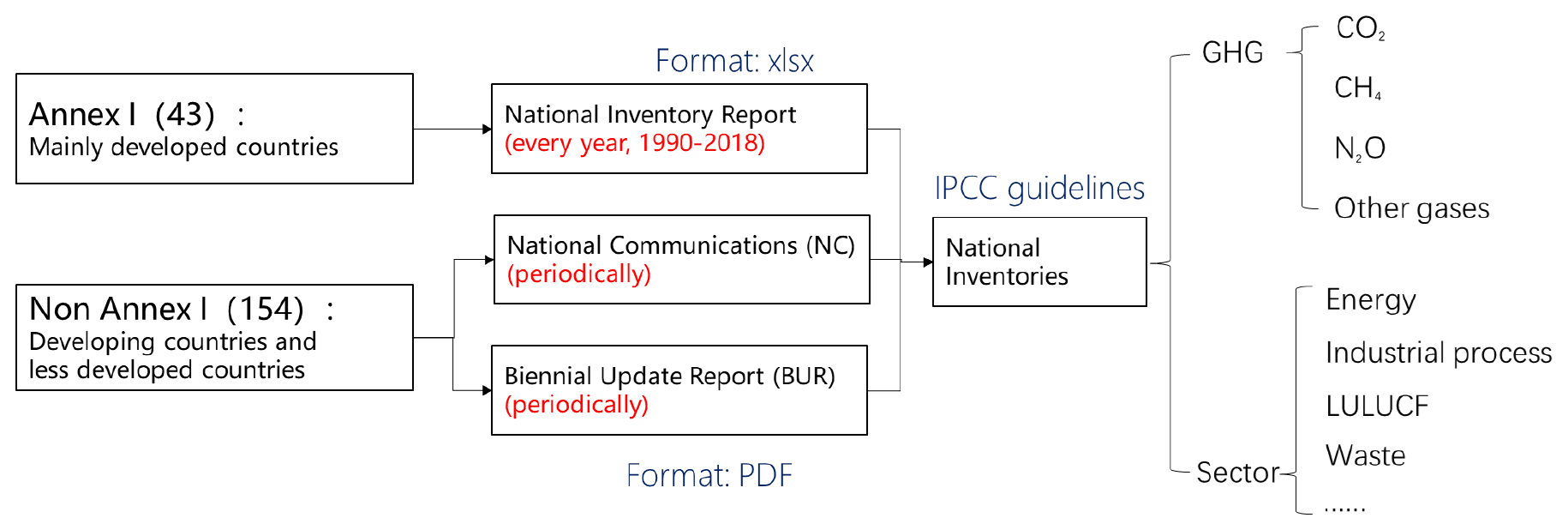
We collected the greenhouse gas emissions data from the national inventories submitted to the UNFCCC. For Annex I countries, data collection is straightforward, as their reports are provided as Excel files under a common reporting format (CRF). For non-Annex I countries, the data were directly extracted from the original reports provided in Portable Document Format (PDF) files. Data from successive reports for the same country were extracted, except when they relate to the same years, in which case only the latest version is considered. While Annex I countries are required to compile their inventory following IPCC 2006 guidelines and the subdivision between sectors established by a UNFCCC decision (dec. 24/CP.19), non-Annex I countries are allowed to follow the older 1996 IPCC guidelines, with different approaches and sectors. Consequently, the methods used and the reported sectors may be different among NC and BUR reports.
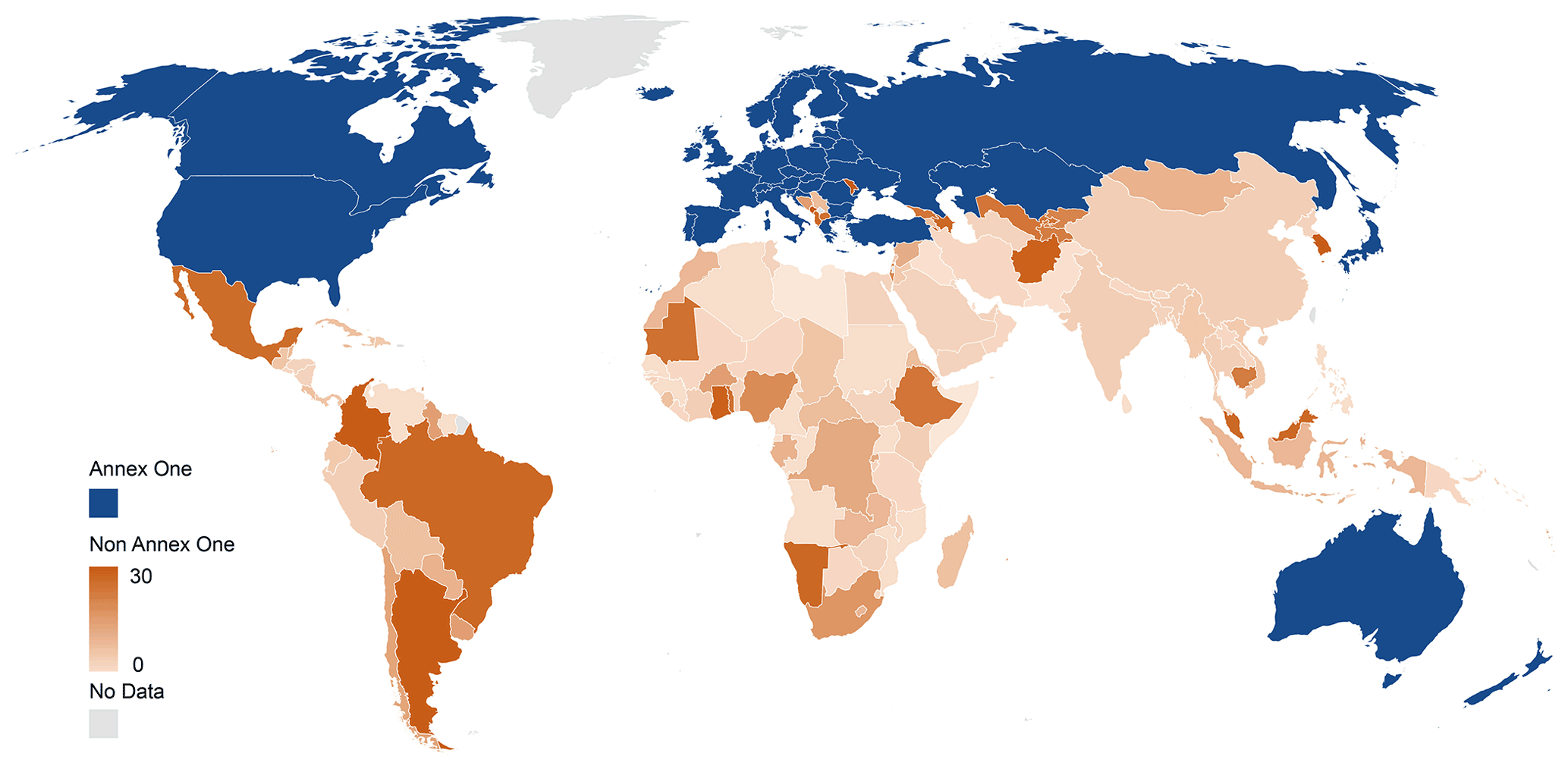
Figure 2Number of reporting years by NGHGI reports (from NCs, BURs, and UNFCCC; detailed data by party, https://di.unfccc.int/detailed_data_by_party, last access: 3 March 2022) which include specific gas and sectoral breakdowns in each non-Annex I country; emissions from Greenland are reported by Denmark.
2.2 Atmospheric inversions
2.2.1 CO2 inversions
The CO2 atmospheric inversions used here (Table S1) are the six from the Global Carbon Budget 2020 (Friedlingstein et al., 2020): CarbonTracker Europe CTE2020 (van der Laan-Luijkx et al., 2017), the Jena CarboScope sEXTocNEET_v2020 (Rödenbeck et al., 2003), the inversion from the Copernicus Atmosphere Monitoring Service (CAMS) v19r1 (Chevallier et al., 2005), the inversion from the University of Edinburgh (UoE) (Feng et al., 2016), the Model for Interdisciplinary Research on Climate (MIROC) inversion (Patra et al., 2018), and the NICAM-based Inverse Simulation for Monitoring CO2 (NISMON-CO2) v2020.1 (Niwa et al., 2017a; Niwa, 2020). They all cover at least the period 2001–2019 based on atmospheric air-sample measurements. Their design is summarized in Tables 4 and A4 of Friedlingstein et al. (2020). A common protocol unites them, but this protocol only deals with the submission procedure and data formats: participants were free to design their inversion configuration in their own way, as long as their resulting inversion satisfied some quality criteria. A common gridded fossil fuel dataset with a monthly resolution (Jones et al., 2021) was made available to the participants as a fixed prior, but its use was not compulsory.
2.2.2 CH4 inversions
The CH4 atmospheric inversions used here (Table S1) to estimate methane fluxes are those from eight inverse systems reporting for the global methane budget (Saunois et al., 2020): CarbonTracker Europe CH4 (Tsuruta et al., 2017), GELCA (Ishizawa et al., 2016), LMDz-PYVAR (Yin et al., 2015; Zheng et al., 2018a, b), MIROC4-ACTM (Patra et al., 2018; Chandra et al., 2021), NICAM-TM (Niwa et al., 2017a, b), NIES-TM–FLEXPART (Wang et al., 2019; Maksyutov et al., 2021), TM5 CAMS (Segers and Houweling, 2017), and TM5 JRC (Bergamaschi et al., 2018). An ensemble of 21 inversions includes 10 surface-based inversions covering 2000–2017 and 11 satellite-based inversions covering 2010–2017 (Table S1). The protocol suggested a set of common prior source and sink estimates along with a set of in situ atmospheric observations. However, their use was not compulsory, and the inversions differ in terms of prior fluxes and handling of observation data. Satellite-based inversion uses TANSO-GOSAT CH4 total columns, but different retrievals were used depending on the modeling group (see Saunois et al., 2020, Supplement). As a result, the ensemble of CH4 inversions derived a wider range of results compared to those from a strict intercomparison protocol. However, most of the inversions were driven using a single prescribed climatological OH from TransCom (Patra et al., 2011). Omitting OH interannual variability and trends leads to attributing most of the variations in atmospheric methane concentration to variations in emissions.
2.2.3 N2O inversions
The N2O atmospheric inversions used to estimate N2O fluxes are the three inversion systems used in the GCP Nitrous Oxide Budget (Tian et al., 2020): GEOS-Chem (Wells et al., 2015), PyVAR-CAMS (Thompson et al., 2014), and INVICAT (Wilson et al., 2014). The MIROC4-ACTM N2O inversion was not used as it has a relatively coarse resolution control vector and appears to be an outlier (Patra et al., 2018). Similarly to CH4, the protocol recommended a set of prior source and sink estimates, but these were not compulsory, although all the three inversions used in this study used the same prior estimates. All inversions used ground-based observations from the NOAA discrete sampling network, and three of the inversions included observations from additional networks (for details see Tian et al., 2020). All inversions accounted for photolysis and oxidation of N2O in the stratosphere, resulting in atmospheric lifetimes in the range of 118 to 129 years.
2.3 Processing of CO2 inversion data for comparison with NGHGIs
2.3.1 National masks – fossil fuel emissions regridding – managed land mask
The aggregation of the gridded flux maps of each inversion, with various native resolutions, at the national annual scale followed the procedure described in Chevallier (2021): it was based on the 0.08∘ × 0.08∘ land country mask of Klein Goldewijk et al. (2017) that allowed us to compute the fraction of each country in each inversion grid box. In addition, for CH4 and N2O, emissions from inland waters at a 0.08∘ × 0.08∘ resolution were attributed to the closest country. For this study, intact forest areas (that are defined as “unmanaged land” in this study) were removed from the CO2 totals, in proportion to their presence in each inversion grid box, based on the intact forest landscape maps of Potapov et al. (2017) shown in Fig. S1. This approach assumes that non-intact forest represents a reasonably good proxy for managed forest reported in national GHG inventories (Grassi et al., 2021). In the absence of a machine-readable definition of the plots considered to be managed in many NGHGIs, this choice remains somewhat arbitrary, and other unmanaged land datasets could have been used (Ogle et al., 2018; Chevallier, 2021). We subtracted the same fossil fuel emissions from Friedlingstein et al. (2020) from the total CO2 flux of each inversion to analyze terrestrial CO2 fluxes, which is equivalent to assuming perfect knowledge of fossil emissions, but note that these values are consistent with the fossil fuel emissions reported in the NGHGIs. This assumption leads to an underestimation of the spread of terrestrial CO2 fluxes among inversions.
2.3.2 Subtracting CO2 fluxes due to lateral carbon transport by crop and wood product trade and by rivers
As defined in the 2006 IPCC Guidelines for National Greenhouse Gas Inventories (IPCC, 2006), only CO2 emissions and removals from managed land are reported in NGHGIs as a proxy for direct human-induced effects. However, inversion models retrieve CO2 fluxes over all land. We thus retained inversions' national estimates of the net ecosystem exchange (NEE) CO2 flux () over managed lands only (ML, here defined as all land except intact forests) because the fluxes over unmanaged land (here approximated by intact forest) are not counted by NGHGIs. Here we use NEE from the definition of Ciais et al. (2020), standing for all non-fossil CO2 exchange fluxes between terrestrial surfaces and the atmosphere; other work may use net biome production (NBP) with a similar meaning. As a result, we produce “adjusted” inversion fluxes that can be compared to inventories. In addition, there are CO2 fluxes that are part of but are not counted by NGHGIs. These fluxes are induced by (i) anthropogenic export and import of crop and wood products across each country's boundary ( and ) and (ii) river carbon export (), which has an anthropogenic and a natural component (Regnier et al., 2013). We assumed that NGHGIs include CO2 losses from fire (wildfire and prescribed fire) and other disturbances (wind, pests) and from harvesting in their estimates of land carbon stocks changes, as recommended by the LULUCF (Land Use, Land-Use Change and Forestry) reporting guidelines. The adjusted inversion NEE that can be compared with inventories, , is given by
where the sign ⇔ means “compared with”, is the anthropogenic CO2 uptake flux from NGHGIs, and is the sum of natural and anthropogenic CO2 uptake flux on land from CO2 fixation by plants that is leached as carbon via soils and channeled to rivers to be exported to the ocean or to another country. All countries export river carbon, but some countries also receive river inputs; e.g., Romania receives carbon from Serbia via the Danube. We estimated the lateral carbon export by rivers minus the imports from rivers entering each country, including dissolved organic carbon, particulate organic carbon, and dissolved inorganic carbon of atmospheric origin distinguished from that of lithogenic origin, by using the data and methodology described by Ciais et al. (2020). Data are from Mayorga et al. (2010) and Hartmann et al. (2009) and follow the approach of Ciais et al. (2020, 2022) proposed for large regions but here with new data at a national scale. Over a country that only exports river carbon, the amount of carbon exported is equivalent to an atmospheric CO2 sink, denoted as as in Eq. (1), thus ignoring burial, which is a small term. Over a country that receives carbon from rivers flowing into its territory, a small national CO2 outgassing is produced by a fraction of this imported flux. In that case, we assumed that the fraction of outgassed to incoming river carbon is equal to the fraction of outgassed to soil-leached carbon in the RECCAP2 region to which a country belongs, estimated with data from Ciais et al. (2020).
is the sum of CO2 sinks and sources induced by the trade of crop products. This flux was estimated from the annual trade balance of 171 crop commodities calculated for each country from FAOSTAT data combined with carbon content values of each commodity (Xu et al., 2021). All the traded carbon in crop commodities is assumed to be oxidized as CO2 in 1 year, neglecting stock changes of products and the fraction of carbon from crop products going to waste pools and sewage waters after consumption, thus not necessarily oxidized to atmospheric CO2. is the sum of CO2 sinks and sources induced by the trade of wood products (Zscheischler et al., 2017). Here, we followed Ciais et al. (2020), who used a bookkeeping model to calculate the fraction of imported carbon in wood products that is oxidized in each country during subsequent years, defined from Mason Earles et al. (2012). Emissions of CO2 by herbivory is partly included in the flux for the fraction of crop products delivered as feed to animals. Emissions of CO2 from grazing animals and their manure decomposition occur in the same grid box as where grass is consumed, so the CO2 net flux captured by an inversion is comparable with grazed grassland carbon stock changes of inventories. Emissions of reduced carbon compounds (VOCs, CH4, CO) are not included in this analysis (see Ciais et al., 2020, for a discussion of their importance in inversion CO2 budgets).
In summary, the purpose of the adjustment of Eq. (1) is to make inversions' output comparable to the NGHGIs that do not include , , and . For example, the UNFCCC accounting rules (IPCC, 2006) assume that all the harvested wood products are emitted in the territory of a country which produces them, which is equivalent to ignoring as a national sink or source of CO2. The adjusted inversion fluxes from Eq. (1) no longer correspond to physical real land–atmosphere CO2 world fluxes, but they match the carbon accounting system boundaries of UNFCCC NGHGIs and will be used in the following. In the following, we will only discuss adjusted inversion CO2 fluxes but for simplicity call them “inversion fluxes”.
2.4 Processing of CH4 inversions for comparison with national inventories
Atmospheric inversions derive net total CH4 emissions at the surface. It is difficult for them to disentangle overlapping emissions from different sectors at the pixel/regional scale based on the information contained in atmospheric CH4 observations only. However, six of the eight modeling systems solve for some source categories owing to different spatio-temporal distributions between the sectors. For each inversion, monthly gridded posterior flux estimates were provided at a 1∘ × 1∘ grid resolution for the net flux at the surface (); the soil uptake at the surface (); the total source at the surface (); and five emitting sectors – agriculture and waste (), fossil fuel (), biomass and biofuel burning (), wetlands (), and other natural () emissions. Considering the soil uptake a “negative source”, the following equation applies:
For inversions solving for net flux only, the partition to source sectors was created based on using a fixed ratio of sources calculated from prior flux information at the pixel scale. For inversions solving for some categories, a similar approach was used to partition the solved categories to the five aforementioned emitting sectors. Such processing can lead to significant uncertainties if not all sources increase or change at the same rate in a given region/pixel. National values have been estimated using the country land mask described in the CO2 section; thus offshore emissions are not counted as part of inversion results unless they are in a coastal grid cell.
Four methodologies were used to separate CH4 anthropogenic emissions from inversions ) in order to compare them with national inventories (). The calculations of anthropogenic emissions by each method were performed separately for GOSAT inversions and in situ inversions. The first method consists in using the inversion partitioning as defined in Saunois et al. (2020):
Method 1
This method has some uncertainties. First, the partitioning relies on the prior estimates, and second, emissions from wildfires are counted for in the biomass and biofuel burning (BB) inversion category but are not reported in NGHGIs. The BB inversion category includes methane emissions from wildfires in forests, savannahs, grasslands, peatlands, agricultural residues, and the burning of biofuels in the residential sector (stoves, boilers, fireplaces). Therefore, we subtracted bottom-up (BU) emissions from wildfires () based on the GFEDv4 dataset (van der Werf et al., 2017) using its reported dry matter burned and CH4 emission factors. The GFEDv4 dataset also reports separately agricultural and waste fire emissions data, which are obviously anthropogenic and occur on managed lands. We assumed that those fires are reported by NGHGIs, so they were not counted in .
Methods 2, 3/1, and 3/2
The second method is a variant of the first one, which removes the median of all inversions of natural emissions (wetlands and other natural sources in Saunois et al., 2020) from the total sources and applies the same removal of wildfires from the BB category as in method 1.
The third method removes natural emissions using only products from bottom-up approaches. This method relies first on the soil uptake (), either prescribed or optimized by each inversion, in order to determine the total methane emissions (anthropogenic + natural).
The bottom-up (BU) natural methane sources removed from total CH4 emissions in Eq. (5) are from separate estimates from termites , wetlands , freshwater (lakes and reservoirs) , and geological processes . Termite emissions are described in Saunois et al. (2020), and we use the mean of their estimates, which amounts to 9 Tg CH4 yr−1 at the global scale. Geological emissions are based on the Etiope et al. (2019) distributions with a global initial total of 37.4 Tg CH4 yr−1 rescaled to a lower value of 5.4 Tg CH4 yr−1 in agreement with pre-industrial radiocarbon CH4 measurements of Hmiel et al. (2020). Freshwater emissions from lakes and reservoirs are from Stavert et al. (2020) and contribute about 71.6 Tg CH4 yr−1 at the global scale, likely an overestimation due to double counting with wetlands (Saunois et al., 2020). It should be noted that fluxes with inland water surfaces are attributed to the closest country by using the high-resolution country mask described in the CO2 section to avoid double counting. Two variants of the third method were used, differing by the bottom-up product used to remove wetland emissions. In method 3/1, we use a climatological estimate of wetland emissions calculated from land surface models forced by the same wetland extent WAD2M (Zhang et al., 2021), and in method 3/2 we use the emissions of the same land surface models simulating variable wetland areas.
2.5 Processing of N2O inversions for comparison with inventories
We subtracted estimates of natural N2O sources from the N2O emission budget ( of each inversion in order to provide inversions of anthropogenic emissions () that can be compared with national inventories ().
For this study, intact forest areas (that are unmanaged, by definition) from Potapov et al. (2017) and lightly grazed grassland areas from Chang et al. (2021a) were removed from the N2O totals in proportion to their presence in each inversion grid box. Lightly grazed grasslands (Chang et al., 2021a) include ecosystems with wild grazers and with extensive grazing by domestic animals, mainly in steppe and tundra regions (Fig. S1). We assumed the intact forest areas and lightly grazed grassland areas approximate unmanaged land, where the fluxes are not reported in the NGHGIs. We verified that the inversion grid box fractions classified as unmanaged do not contain point source emissions from the industry or energy and diffuse emissions from the waste sector to make sure that we do not inadvertently remove anthropogenic sources by masking those unmanaged areas.
To do so, from the EDGAR v4.3.2 inventory (Janssens-Maenhout et al., 2019), we checked that N2O from waste water handling covers a relatively large area that might be partly located in unmanaged land. But the emission rates are more than 1 order of magnitude smaller than those from agriculture soils. For other sectors, only very few of the unmanaged grid boxes contain point sources, and none of them has an emission rate that is comparable with agricultural soils (managed land). Thus, our assumption that emissions from these other sectors are primarily located over managed land is solid (other sectors include power industry; oil refineries and transformation industry; combustion for manufacturing; aviation; road transportation, no resuspension; railways, pipelines, and off-road transport; shipping; energy for buildings; chemical processes; solvents and product use; solid waste incineration; waste water handling; and solid waste landfills). Therefore, our masking of unmanaged land inversion grid boxes gives us in Eq. (6). The flux is the natural emissions from freshwater systems in Eq. (6) given by a gridded simulation of the DLEM (Yao et al., 2019) describing pre-industrial N2O emissions from N leached by soils and lost to the atmosphere by rivers in the absence of anthropogenic perturbations (considered the average of 1900–1910). Natural emissions from lakes were estimated only at a global scale by Tian et al. (2020) and represent a small fraction of rivers' emissions. Therefore, they are neglected in this study. The flux is based on the GFED4s dataset (van der Werf et al., 2017) using their reported dry matter burned and N2O emission factors. Because the GFED dataset reports specific agricultural and waste fire emissions data and we assume that those fires (on managed lands) are reported by NGHGIs, they were not counted in . Note that there could also be a background natural N2O emission from soils over managed lands (). We did not try to subtract this flux from managed land emissions because we assumed that, after a land use change from natural to fertilized agricultural land, background emissions decrease and become very small compared to N-fertilizer-induced anthropogenic emissions. In a future study, for we could use the estimate given by simulations of pre-industrial emissions from the NMIP ensemble of dynamic vegetation models with carbon–nitrogen interactions (number of models, n, is 7), namely, its simulation S0 in which climate forcing is recycled from 1901–1920, CO2 is at the level of 1860, and no anthropogenic nitrogen is added to terrestrial ecosystems (Tian et al., 2019).
Another important point to ensure a rigorous comparison between inversions and NGHGI data is whether anthropogenic indirect emissions (AIEs) of N2O are reported in NGHGI reports. UNFCCC parties should report these in their NGHGIs according to the IPCC guidelines, but we found that this is not always the case. For example, South Africa's BUR3 did not report the indirect GHG emissions. AIEs arise from anthropogenic nitrogen from fertilizers leached to rivers and anthropogenic nitrogen deposited from the atmosphere to soils. AIEs typically represent 20 % of direct anthropogenic emissions and cannot be ignored in a comparison with inversions. For Annex I countries, AIEs are systematically reported, generally based on ad hoc emission factors since these fluxes cannot be directly measured, and it is assumed that indirect emissions only occur on managed land. For non-Annex I countries, we checked manually from the original NC and BUR documents if AIEs were reported or not by each non-Annex I country. If AIEs were reported by a country, they were used as such to compare NGHGI data with inversion results and grouped into the agricultural sector. If they were not reported or if their values were outside plausible ranges, AIEs were independently estimated by the perturbation simulation of N-fertilizer leaching, CO2, and climate on rivers and lakes fluxes in the DLEM (Yao et al., 2019) and by the perturbation simulation of atmospheric nitrogen deposition on N2O fluxes from the NMIP model ensemble (Tian et al., 2019). Table S2 lists the non-Annex I countries among the top 20 N2O emitters if they have reported AIEs to the UNFCCC from national inventories.
2.6 Grouping of inventory sectors for comparison with inversion sectors
The categories of fluxes estimated by inversions and NGHGI sectors are different (Table S3). The bottom-up inventories are compiled based on activity data (statistics) following the IPCC 1996 and 2006 guidelines (IPCC, 1997, 2006), with detailed information of sub-sectors. But the top-down inversions can only distinguish very few sectors. Thus, in this study, we aggregated sectors into some larger sectors to make inversions and inventories comparable for each GHG gas (Table 1).
For CO2, the inversions are divided into two aggregated sectors: (1) fossil fuel and cement CO2 emissions and (2) land flux. Inversions use a prior gridded fossil fuel dataset as summarized in Sect. 2.2; thus, in this study we compare only the land flux between inversions and inventories. The adjusted land flux (NEE) from each inversion is calculated by subtracting the national total fossil emissions from the total CO2 flux, where the fossil emissions are from the Global Carbon Project annual dataset (Friedlingstein et al., 2020), consistent with the prior fossil emission maps proposed to inversion modellers and used by them, except for the inversion of Feng et al. (2009, 2016) (see Table A4 of Friedlingstein et al., 2020, for details). For processing NGHGIs, we subtracted fossil emissions of the sectors of energy and industrial processes (or industrial processes and product use) from the total net CO2 emissions to obtain NEE CO2 fluxes over managed ecosystems. Note that transportation and residential CO2 emissions are reported under the energy sector.
For CH4, we compare inversions and national inventories based on three emission groups: fossil, agriculture and waste, and total anthropogenic. For NGHGIs, we group the sectors of energy and industrial processes (and product use) into fossil, excluding biofuel burning (reported under the energy sector); group sectors of agriculture and waste into agriculture and waste; and aggregate fossil, agriculture and waste, and biofuel burning into total anthropogenic.
For N2O, we derived anthropogenic emissions by Eq. (6) by subtracting natural emissions from rivers from Yao et al. (2019) after masking unmanaged grasslands and intact forest areas.
Table 1Grouping of aggregated sectors for comparisons between inventories and inversions.
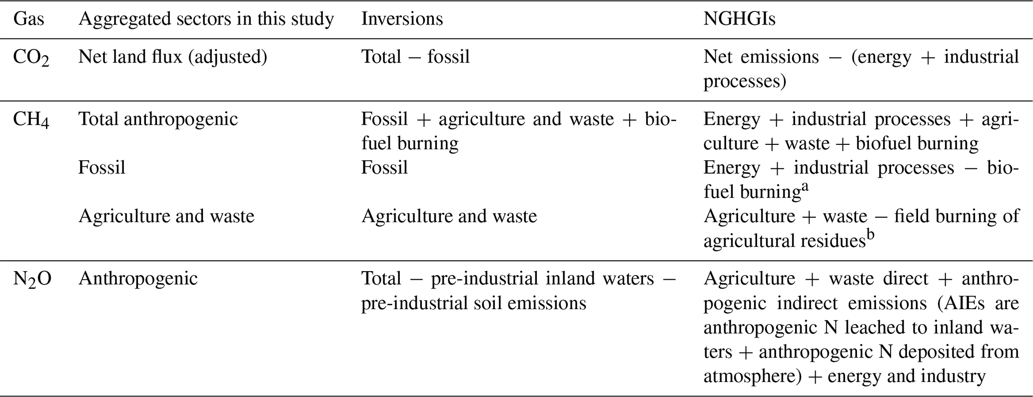
a Biofuel burning is likely not included in NGHGIs but is under “1 A 4 Other Sectors” if it is reported. b Field burning of agricultural residues is reported in Annex I countries under the agricultural sector. Note that indirect N2O emissions are reported by Annex I countries but not systematically by non-Annex I ones (see Table S2).
2.7 Choice of example countries for analysis
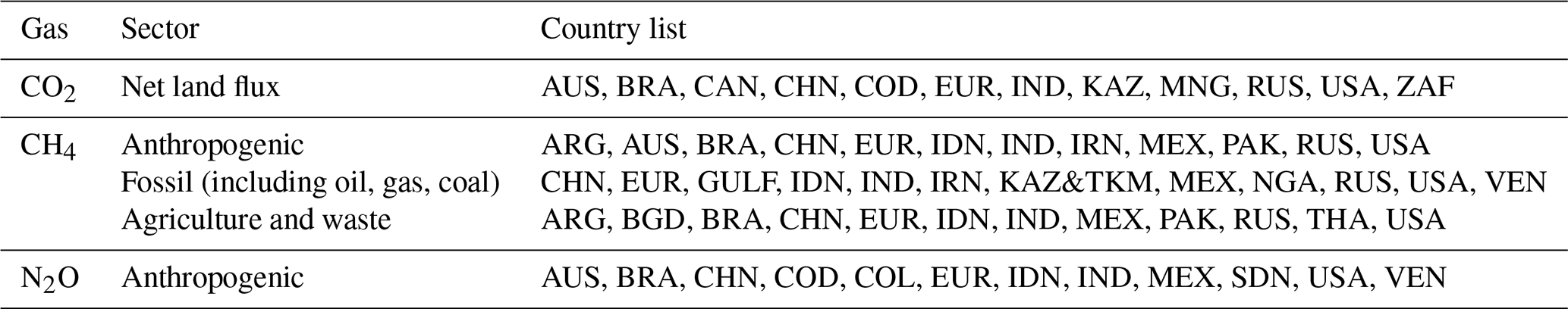
We selected 12 countries (counting the EU27 and UK as 1 country) for the analysis, the selection being different for CO2, CH4, and N2O anthropogenic fluxes, based on the following criteria. Each selected country should have a large enough area because small countries cannot be constrained using coarse-spatial-resolution inversions and, if possible, some coverage by the in situ global network. The country with the smallest area is Venezuela (916 400 km2), selected for CH4 because it is a large oil and gas emitter and its emissions can still be constrained by inversions using GOSAT satellite observations, except inversions using the NIES column CH4 product that has very few observations in the wet season over Venezuela and Nigeria for instance (see Table S1 and Fig. S2 for GOSAT satellite sounding coverage). For CO2, we selected the top 10 fossil fuel CO2 emitters because, even if inversions do not resolve those emissions which are used as a fixed prior, it is important to compare the magnitude of their CO2 sinks with their fossil CO2 emissions. We also selected two large boreal countries (i.e., Russia and Canada); two tropical countries with important areas of forests (i.e., Brazil and the Democratic Republic of Congo); two large countries with in situ stations (i.e., Mongolia and Kazakhstan); and two large dry Southern Hemisphere countries with a high rank in the fossil fuel CO2 emitters (i.e., South Africa and Australia), which both have atmospheric stations to constrain their land CO2 flux. Altogether, the 12 countries account for >90 % of the global land CO2 sink given by NGHGIs. For CH4, we ranked countries or groups of countries in decreasing order of total anthropogenic, fossil, and agricultural emissions. The criteria of large areas and having atmospheric stations are important for in situ inversions. For satellite inversions, the advantage of GOSAT is that it provides observations where the surface network is very sparse, such as the tropics, so that countries with no or only a few ground-based observations can still obtain reliable top-down estimates. The inversion resolution is what dictates if small countries can be reliably estimated. Thus, this study includes China, India, the USA, the EU, Russia, and Indonesia, which are among the top fossil and top agricultural emitters and have vast territories, and excludes small countries considering the coarse spatial resolution. Altogether, the selected countries for CH4 represent ∼60 % of the global anthropogenic CH4 emission given by NGHGIs, ∼15 % of the fossil emissions, and ∼40 % of agriculture and waste emissions. For N2O, we chose the top 12 emitters based on NGHGI reports. In most of them, anthropogenic N2O emissions are dominated by the agricultural sector, whose share (including indirect agricultural emissions) of total NGHGI emissions ranges from 6 % in Venezuela to 95 % in Brazil. Altogether, the selected countries represent ∼55 % of the global anthropogenic N2O emissions given by NGHGIs.
Table 2Lists of countries or groups of countries analyzed and displayed in the result section for each gas and each sector: China (CHN); the United States (USA); Russia (RUS); Canada (CAN); Kazakhstan (KAZ); Mongolia (MNG); India (IND); Brazil (BRA); the Democratic Republic of the Congo (COD); South Africa (ZAF); Australia (AUS); the EU27 and UK – the 27 member states of the EU and the United Kingdom (EUR), Pakistan (PAK), Argentina (ARG), Mexico (MEX), Iran (IRN), Indonesia (IDN); Saudi Arabia, Oman, the United Arab Emirates, Kuwait, Bahrain, Iraq, and Qatar (GULF); Kazakhstan and Turkmenistan (KAZ&TKM); Venezuela (VEN); Nigeria (NGA); Thailand (THA); Bangladesh (BGD); Colombia (COL); and Sudan (SDN).
First, we compared the global land use CO2 flux from inversions with NGHGIs. While data for the specific countries analyzed in this paper (Fig. 3) are based on our own compilation, the global land use flux from NGHGIs is from Grassi et al. (2021) (based on a compilation of different country submissions to the UNFCCC, in a few cases gap-filled with country reports to FAO Global Forest Resources Assessment (FRA) 2015). For the period 2007–2017, our inversions give an average global land sink of 1.4 Gt C yr−1 over all lands and of 1.3 Gt C yr−1 over managed lands. Over managed lands, the CAMS, UoE, and Jena models have a higher sink; CTE2020 and NISMON give similar values; and MIROC gives a smaller sink than over all lands (see Table S1 for the list of models). For a similar period (2010 and 2015) the NGHGI data compiled by Grassi et al. (2021) indicate a global land sink of only 0.3 Gt C yr−1, which is much smaller than that of inversions. Such a large difference can be possibly explained by the fact that (i) NGHGIs are incomplete, especially in developing countries, especially for soil carbon stock change in grasslands, croplands, wetlands, and forests (where actual observation-based estimates are often lacking) and (ii) in some cases, NGHGIs do not fully capture recent environmental effects (e.g., CO2 fertilization). Inversions are also smaller than the Tier 1 approach published by Harris et al. (2021), who estimate a sink of 2.1 Gt C yr−1 over the last 20 years over managed and unmanaged forests, with a large range of ±13 Gt C that seems biophysically implausible.
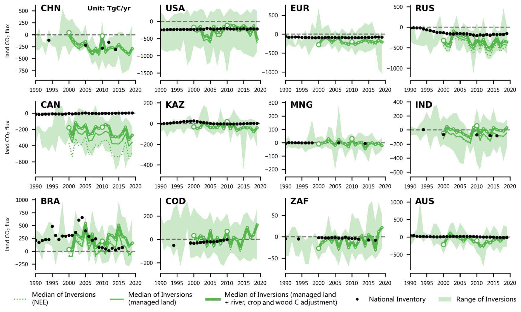
Figure 3Net ecosystem exchange (NEE) CO2 fluxes (Tg C yr−1) from China (CHN), the United States (USA), the EU27 and UK (EUR), Russia (RUS), Canada (CAN), Kazakhstan (KAZ), Mongolia (MNG), India (IND), Brazil (BRA), the Democratic Republic of the Congo (COD), South Africa (ZAF), and Australia (AUS). By convention, CO2 removals from the atmosphere are counted negatively, while CO2 emissions are counted positively. The black dots denote the reported values from NGHGIs. Note that C stock change for agricultural land is reported under the LULUCF sector, whereas CH4 and N2O emissions of agricultural activities are reported in the agriculture sector. The fossil emissions CO2 from agricultural machinery are reported under the energy sector and not included under the agriculture sector or the AFOLU (Agriculture, Forestry, and Other Land Use) sector. For EUR, the NISMON inversion data were removed in 2018 and 2019, being a large outlier. The thick solid green lines denote the median of land fluxes over managed land of all CO2 inversions, after adjustment of CO2 fluxes from lateral transport by rivers and crop and wood trade. The thin solid line is the median of inversions over managed land and without lateral transport adjustment. The dotted line is the original median of inversions, where the large hollow dots in the line are for years beginning a decade and small hollow dots are for other years. Light green shading is from the min–max range of inversions. Because before 2000, there were only four inversion models, the median is not shown.
Figure 3 displays the time series of land-to-atmosphere CO2 fluxes for the selected countries (Table 2). Across the 12 countries, the median of inversions shows significant interannual variability, generally consistent between the six inversions (Fig. S3). This signal reflects the impact of climate variability on terrestrial carbon fluxes and of annual variations in land use emissions. In the inversion of CO2 fluxes, the effects of climate variability on an interannual and decadal scale, rising CO2, nitrogen availability, and other environmental drivers are not separable from the direct human-induced effects of land use and management. Decadal variability in carbon stocks induced by climate and environmental drivers is mostly captured by the NGHGIs of countries that use regular forest inventories to measure stock changes over time (stock-difference method), e.g., with dense sampling of forest plots. Yet, such gridded stock change inventories do not capture interannual variability, for instance, when higher mortality or a growth deficit occurs in a severe drought year and causes an abnormal CO2 source to the atmosphere (Ciais et al., 2005; Wolf et al., 2016; Bastos et al., 2020). In contrast, the NGHGIs of countries based on forestry models using static growth curves of representative forests do not necessarily capture the recent transient impact of environmental driver changes; see Table 1 in the Supplement of Grassi et al. (2021), which includes information on the method (gain–loss or stock difference) used by several major countries. This may partially explain why inversions estimate higher CO2 sinks (e.g., in CAN, AUS, and some EUR countries).
In large fossil CO2 emitter countries of temperate latitudes, inversions and NGHGI estimates are quite similar in China (CHN) and the USA but give a higher CO2 uptake in the EU27 and UK (EUR), Russia (RUS), and Canada (CAN) (Fig. 3). In these five countries/group of countries, adjusting inversions by CO2 fluxes induced by river carbon transport and by the trade of crop and wood products tends to lower CO2 sinks, especially for large crop exporters like the USA and CAN. But it still leaves a median CO2 uptake after adjustment (of 243 Tg C yr−1 in CHN, 243 Tg C yr−1 in the USA, 189 Tg C yr−1 in EUR, 325 Tg C yr−1 in RUS, and 217 Tg C yr−1 in CAN during 2000–2019) which is still higher than in NGHGI reports (Fig. 3). The differences between NGHGIs and inversions differ between countries however.
In CHN, the successive national communication estimates in five different years fall in the range of the six inversions and give a trend towards an increasing carbon sink. Adjusted inversions provide a median CO2 sink of 142 Tg C yr−1 in 2005 and of 245 Tg C yr−1 during 2010–2014, consistent with reported values from NGHGI reports (166 Tg C yr−1 in 2005 and an average of 247 Tg C yr−1 in 2010, 2012, and 2014). Note that the NGHGIs in 2010 and 2014 reported in China's NC3 and BUR2 used the IPCC 2006 guidelines to calculate the flux from the LULUCF sector, which includes fluxes from six land use types (forest land, cropland, grassland, wetlands, settlements, and other land). However, the LULUCF sector in the previous 3 years reported in NC1, NC2, and BUR1 only considered fluxes from forest land.
In the USA, the carbon stock change estimates of the NGHGIs fall within the range of inversions during the last 3 decades, with a mean value of 221 Tg C yr−1 from NGHGIs during 2000–2019 compared to an average of 243 Tg C yr−1 by inversions (going from a sink of 943 Tg C yr−1 to a source of 286 Tg C yr−1). Yet, the USA inventory gives a small decrease in carbon sinks with time, whereas the median of adjusted inversions produces a decrease in the net CO2 uptake, from an average of 287 Tg C yr−1 in the 2000s to 200 Tg C yr−1 in the 2010s, dropping by nearly 30 % during the last 30 years despite the uncertainty suggested by the range of inversion model results. Estimates from NGHGIs also show a decreasing trend but with less fluctuation, from a mean value of 239, 222, and 219 Tg C yr−1 in the 1990s, 2020s, and 2010s, respectively. In EUR, inversions systematically indicate a larger net CO2 uptake than NGHGIs, by on average 104 Tg C yr−1 more than NGHGIs yet with a non-significant trend (Mann–Kendall test p=0.7), consistent with stable land carbon storage shown by NGHGIs.
In the two largest boreal and Arctic countries Canada (CAN) and Russia (RUS), inversions produce a CO2 sink (average 217 and 325 Tg C yr−1) which is systematically larger than that of the NGHGIs (2 and 171 Tg C yr−1, respectively) during 2000–2019. CAN is one of the few countries that does not capture most of the recent indirect environmental change effects (Grassi et al., 2021). The larger Russian sink of inversions is similar to the results of a recent analysis (Schepaschenko et al., 2021) of forest inventory and satellite biomass data estimating a carbon accumulation of 343 Tg C yr−1 from 1988 to 2014. The Russian carbon sink rate of increase is 6.0 Tg C yr−2 in the NGHGIs during the 2000s, smaller than the increasing CO2 sink rate of 16.4 Tg C yr−2 across inversions. When inversions include all lands in these two countries instead of managed land only, the net land CO2 sink becomes 40 % larger in CAN and 16 % larger in RUS. Unmanaged lands in our intact forest dataset cover 30 % of CAN and 15 % of RUS total forest area and are associated with CO2 sink densities of 44 and 29 g C m−2 yr−1, respectively, nearly identical to 46 and 30 g C m−2 yr−1 in managed lands. It should be noted that in Canada's CRF, removals by forest land are largely diminished by the emissions from harvested wood products in the LULUCF sector.
Among the selected large forested tropical countries, Brazil (BRA) is one of the few non-Annex I countries that has provided continuous time series of NGHGIs since 1990. The Brazilian NGHGIs show a net loss of carbon stocks from 1990 to 2020, with an increasing loss from 1990 to 2005 followed by a decrease afterwards. This change is explained mostly by deforestation rates (tree cover loss), which declined by a quarter between 2001–2005 (3.4 Mha yr−1) and 2006–2016 (2.7 Mha yr−1) (Global Forest Watch, 2021) or from 5.1 Mha yr−1 in 2000–2010 to 1.7 Mha yr−1 in 2015–2020, following government policies to protect forests, which were enforced until 2019. The latest year of reported inventory was 2016 in BRA, but satellite estimates of deforestation rates in the Brazilian Amazon from the Program to Calculate Deforestation in the Amazon (PRODES) system of the Brazilian Space Agency indicated a sharp increase in deforestation in 2019 (1 Mha). On top of deforestation, degradation and fires also cause a loss of carbon in BRA and other Amazon countries, such as Peru (18 Tg C yr−1 during 2000–2019) and Colombia (25 Tg C yr−1 during 2000–2019). The area of degraded forests has been reduced in BRA, tailing off with the reduction trend of deforestation until 2019 (Bullock et al., 2020; Matricardi et al., 2020), even though the components of degradation from burned and logged forests, two processes causing the largest loss of carbon per unit area, have remained constant over time. The number of active fires in BRA seems to have remained constant, with peaks during dry years. The CO2 emissions from fires may be larger and decoupled from decreasing CO2 losses from decreasing deforestation (Aragão et al., 2018). Drought generally causes abnormal CO2 losses in the Brazilian Amazon, of 0.48 Gt C yr−1 during the 2010 drought, based on a regional inversion with aircraft CO2 vertical profiles (Gatti et al., 2014), and of 0.25 Gt C yr−1 during the extreme El Niño drought of 2015, from aboveground biomass loss estimated by satellite vegetation optical depth changes (Qin et al., 2021). The land fluxes of inversions indicate that Brazilian managed land became abnormal sources in the dry years 2005 (540 Tg C yr−1), 2007 (334 Tg C yr−1), 2010 (195 Tg C yr−1), and 2015 (511 Tg C yr−1), with a sudden net increase compared to the previous year (240 Tg C in 2004, 180 Tg C in 2006, 132 Tg C in 2009, and 232 Tg C in 2015). Over the period 2010–2019, the aboveground net mean CO2 flux of the Brazilian Amazon area was estimated to be a weak source of 0.06 Gt C yr−1 (Qin et al., 2021), also consistent with data from the inversion of Palmer et al. (2019) (see their Table 1). The median land CO2 flux of inversions in this study over the same period shows a source of 0.25 Gt C yr−1, comparable in magnitude but with a large spread (from a small sink of 96 Tg C yr−1 to a source of 510 Tg C yr−1). Recently, a top-down estimate based on 2010–2018 aircraft profiling of CO2 mole fractions (Gatti et al., 2021) suggested a substantial source of carbon in the eastern Amazon forest basin driven by fire emissions and loss of forest carbon uptake in dry seasons. The western part of the basin was nearly neutral in NEE, with deforestation fires and climate warming/drying playing a much smaller role. We also acknowledge that the estimate by Qin et al. (2021) gives only the carbon change in aboveground biomass, which is not strictly comparable to inversion results, the latter including soil and inland water CO2 fluxes and legacy CO2 emissions following mortality from the decomposition of coarse woody debris (Yang et al., 2021). Note also the importance of lateral carbon fluxes from the export of agricultural commodities in Brazil as a driver of deforestation (Follador et al., 2021; Weisse and Goldman, 2021). As for the other selected large forested tropical country, the Democratic Republic of Congo (COD), NGHGIs show a net sink of 19 Tg C yr−1 from 2000 to 2010 with a smaller interannual variability than in BRA despite a similar forested area. Interestingly, NGHGIs in COD show a decreasing CO2 sink from 1994 to 2010, while inversions give an increasing CO2 sink from the 1990s to the period around 2010, followed by a reversal after 2010. During the last decade, years after 2015 were net CO2 sources to the atmosphere for COD. It should be acknowledged that the NGHGIs of COD are extremely uncertain (and contradictory information, i.e., high removals, has been provided by the country in different official documents sent to the UNFCCC and to FAO).
For India (IND), although the land CO2 sinks show an increased uptake across inversions during the first half of the 2000s with an annual uptake of 14 Tg C yr−1 during this period, the CO2 uptake from the inversions fluctuated between positive and negative values in the 1990s and 2010s, indicating that the role of land CO2 flux shifted between a net carbon sink and a net carbon source (Takaya et al., 2021). This shift to a net CO2 source could be explained by a decreased Indian monsoon after ∼2007 (University of Hawaii Indian Summer Monsoon Index, http://apdrc.soest.hawaii.edu/projects/monsoon/seasonal-monidx.html, last access: 5 July 2021). For the two continental Asian countries, Mongolia (MNG) and Kazakhstan (KAZ), the land CO2 flux fluctuates around zero with a small interannual variation, indicating a stable trend of land flux changes and a small contribution to the uptake of all Northern Hemisphere Annex I countries.
For Australia (AUS), there is a clear CO2 sink anomaly during the extremely wet La Niña event from May 2010 to March 2012 (Poulter et al., 2014; Haverd et al., 2016). In the following fire season of late 2012 and early 2013, more fires were reported from the legacy of a higher fuel load in the previous wet period, and these CO2 emissions likely caused the net CO2 uptake to decrease (Harris and Lucas, 2019).
For maritime Southeast Asian countries, that is, Indonesia (IDN), Malaysia (MYS), and Papua New Guinea (PGN) grouped together (Fig. S4), we found a large peak of CO2 emissions during the El Niño of 1998 corresponding to extreme fire emissions from peat burning (Page et al., 2002). This group of countries shows a net sink of 60 Tg C yr−1 of CO2 since 2000. For continental Southeast Asian countries, that is, Thailand (THA), Myanmar (MMR), Laos (LAO), Cambodia (KHM), and Viet Nam (VMN) grouped together, we found on average that inversions give a similar net CO2 flux to that reported by NGHGIs. In this group of countries, inversions give a decreasing sink trend in the last decade (Fig. S4), consistent with the observation of increased forest clearing and biomass carbon losses, in particular over mountain regions (Davis et al., 2015; Zeng et al., 2018).
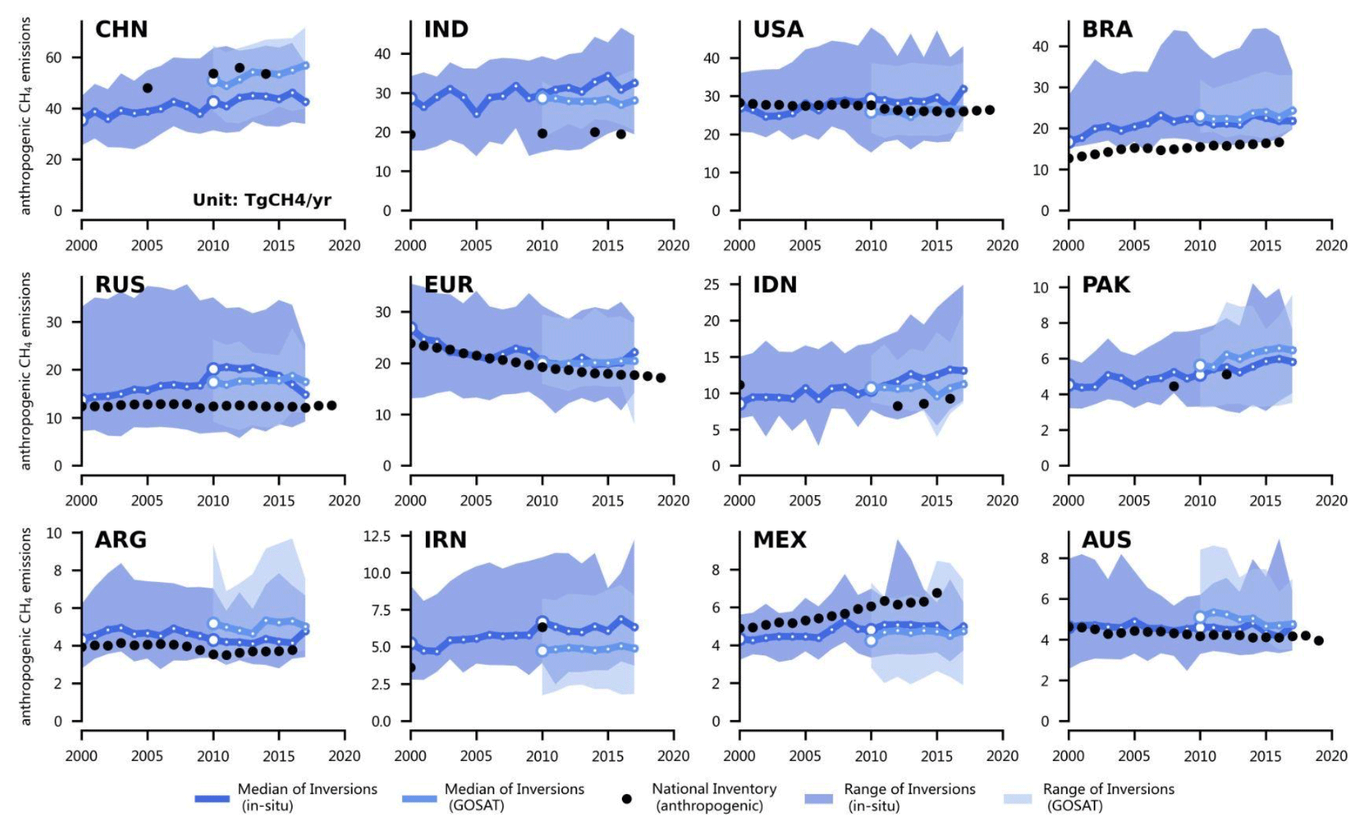
Figure 4Total anthropogenic CH4 fluxes for the 12 top emitters: China (CHN), India (IND), the United States (USA), Brazil (BRA), Russia (RUS), the EU27 and UK (EUR), Indonesia (IDN), Pakistan (PAK), Argentina (ARG), Iran (IRN), Mexico (MEX), and Australia (AUS), following method 1 based on the original separation of anthropogenic vs. natural sources by each inversion with wildfires subtracted (see Sect. 2). The black dots denote the reported values from NGHGIs. The dark blue lines and areas denote the median and maximum–minimum ranges of in situ CH4 inversions, respectively, and the light blue ones the equivalent of the GOSAT inversions. Note the different scale for each country.
4.1 Total anthropogenic CH4 emissions
Figure 4 shows the variations in CH4 anthropogenic emissions from 2000 to 2019 (up to 2017 for inversions), defined by summing the sectors of agriculture and waste, fossil fuels, and biofuel burning for the 12 selected countries (see Sect. 2.4). The distribution of emissions is strongly skewed even among the top 12 emitters, with the largest and most populated countries forming a group of super-emitters and other countries having much smaller emissions and thus being more difficult to quantify by inversions. According to GOSAT inversions, China (CHN) has the largest emissions of around 53 Tg CH4 yr−1, followed by India (IND) with 28 Tg CH4 yr−1, the USA with 26 Tg CH4 yr−1, Brazil (BRA) with 23 Tg CH4 yr−1, the EU27 and UK (EUR) with 20 Tg CH4 yr−1, Russia (RUS) with 18 Tg CH4 yr−1, and Indonesia (IDN) with 11 Tg CH4 yr−1, and the other countries has emissions of only around 5 Tg CH4 yr−1. Note the asymmetric range around the median of inversions for BRA in Fig. 4. The data in Fig. 4 indicate a large spread between inversions, owing to differences in model settings and transport. Differences due to different methods used to separate anthropogenic from natural emissions are smaller than this spread, and we discuss them in Sect. 6.2. We observed on average a smaller range of GOSAT inversions (number of inversions, n is 11) than in situ inversions (n=10) in countries emitting more than 10 Tg CH4 yr−1. The median emissions from GOSAT inversions are systematically lower than from in situ inversions, except in CHN where GOSAT inversions are on average 21 % larger than in situ ones during 2010–2017. Ranges overlap between the two inversion ensembles. Generally, the difference between NGHGIs and inversions is of the same sign based on GOSAT and in situ inversions, which gives us some confidence for evaluating NGHGIs because the GOSAT observations are different and independent from in situ networks. Ex ante, we trust more GOSAT-based inversions over most countries because GOSAT has a better observation coverage, except for in EUR and the USA where the in situ network is dense (Fig. S2). From the result shown in Fig. 4 that GOSAT and in situ inversions are on the same side compared to NGHGIs, we can thus be more confident of results provided by in situ inversions over the full time period.
For China (CHN), during 2000–2017, the median of anthropogenic emissions from in situ inversions is 44 Tg CH4 yr−1. This is lower than the NGHGI reports (53 Tg CH4 yr−1, average of four communications in 2005, 2010, 2012, and 2014). The median of GOSAT inversions (53 Tg CH4 yr−1) is close to that of NGHGIs (54 Tg CH4 yr−1) in the 2010s (Fig. 4). The trend of emissions is consistent between inversions and NGHGI data, although the increasing trend is larger in GOSAT than in in situ inversions after 2010. For the USA, the median of inversions is close to the NGHGI-reported value during the whole study period. The trend of in situ inversions in the USA is positive, with an increase of 0.3 Tg CH4 yr−1 from 2000 to 2017, in contrast to the small decrease of 0.1 Tg CH4 yr−1 in the NGHGI data. The GOSAT inversions also show a positive trend of 0.1 Tg CH4 yr−1 from 2010 to 2017. This different trend between inversions and the US NGHGIs might be attributed to CH4 leakage from unconventional oil and gas extraction that may not be fully accounted for in NGHGIs (Allen, 2016). This type of oil and gas production became important after the mid-2000s and has emission factors that are twice larger than current values from the US Environmental Protection Agency (EPA) currently used in the NGHGIs, as shown by local and regional measurement campaigns (Alvarez et al., 2018; Sargent et al., 2021).
For the EU27 and UK (EUR), the decreasing trend of anthropogenic CH4 emissions diagnosed by inversions is consistent with NGHGI estimates, but the median of inversions is higher than the NGHGI data by 2 Tg CH4 yr−1 for the study period from 2010 to 2017. This result is consistent with the EU synthesis results of Petrescu et al. (2021b) although they used a different method to subtract natural emissions based on regional estimates of peatlands and inland water natural emissions. Positive differences between inversions and NGHGI reports are found for Russia (RUS), India (IND), Brazil (BRA), Argentina (ARG), and Australia (AUS). In Russia (RUS), emissions are larger in inversions than in the NGHGI data, and this result is robust to the choice of the method to separate natural from anthropogenic sources (see Figs. S5 and 10). Note however that RUS wetland emissions are partly concentrated in the region of western Siberia (northern Ob river basin) just to the south of a major basin of gas extraction (Yamal), and these two sources are difficult to separate from each other in global inversions. Note that methane emissions from fires in Russia are smaller than fossil and wetland emissions, and fires cannot explain why inversions give larger emissions than the NGHGIs.
In Brazil (BRA), the result that inversions give systematically larger CH4 emissions than NGHGIs is also robust due to the method used to separate wetlands from anthropogenic emissions (Fig. S5), but our inversions did not use in situ data in the interior of the country (Fig. S1) and the coverage of GOSAT is sparse due to clouds (Fig. S2), especially in the wet season, which makes the estimation of the total CH4 source uncertain over this country. In India (IND), both the in situ and the GOSAT inversions also give a higher anthropogenic emission than the NGHGI data and the share of emissions from natural wetlands is much smaller than in RUS and BRA, reducing the risk of aliasing between anthropogenic and natural emissions and suggesting a lower estimation by the NGHGIs. In Indonesia (IDN) the median of inversions is slightly higher than the NGHGI data with the separation method used in Fig. 4 but close to NGHGIs with other methods (Figs. 10 and S5). All inversions give a large positive anomaly of CH4 emissions during the 2015 El Niño, when abnormal peat fire emissions occurred (Heymann et al., 2017; Yin et al., 2016), with a biomass burning event being attributed to an anthropogenic source by our aggregation of inversion results (Sect. 2) but likely not included by the NGHGIs. In AUS, the anthropogenic emissions mainly from the coal extraction and cattle sector of the NGHGIs are found to be very close to the inversion median, across both in situ and GOSAT inversions. In Pakistan (PAK) and Iran (IRN), NGHGI values show good consistency with the in situ inversions; however, in Pakistan (PAK) the GOSAT inversions are 18 % higher than the in situ inversions. Mexico (MEX) is the only country whose NGHGIs are higher than the inversions among the 12 selected countries, which is mainly attributed to the difference between inversions and inventories in the agriculture and waste sector (see below).
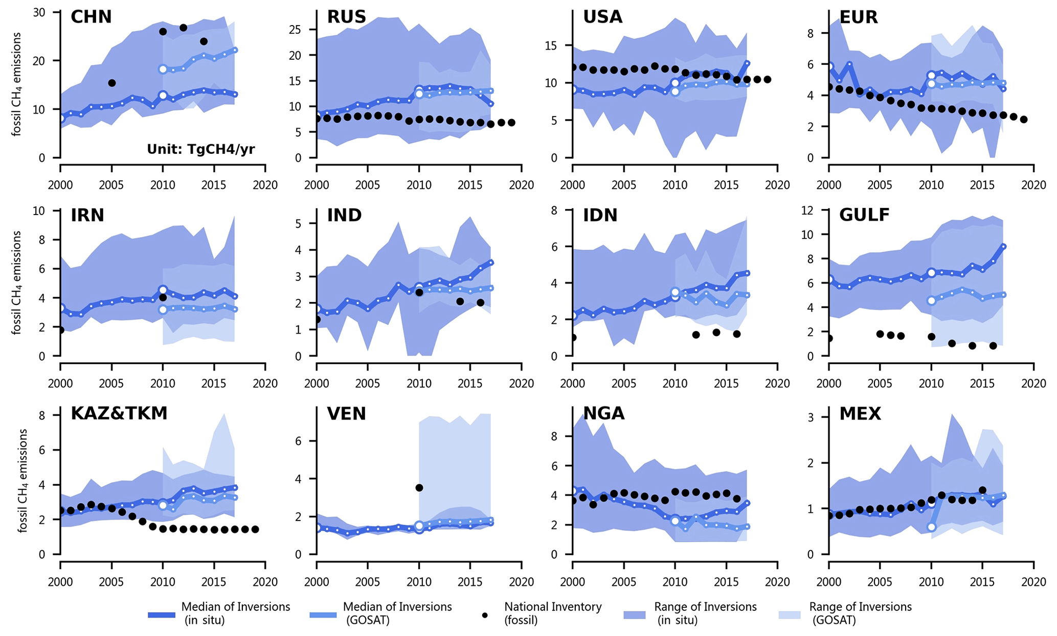
Figure 5CH4 emissions from the fossil fuel sector from the top 12 emitters of this sector: China (CHN), Russia (RUS), the United States (USA), the EU27 and UK (EU), Iran (IRN), India (IND), Indonesia (IDN), Persian Gulf countries (GULF denotes Saudi Arabia + Iraq + Kuwait + Oman + the United Arab Emirates + Bahrain + Qatar), Kazakhstan and Turkmenistan (KAZ&TKM), Venezuela (VEN), Nigeria (NGA), and Mexico (MEX). The black dots denote the reported value from the NGHGIs. In the NGHGI data shown in Fig. 5 for GULF, Saudi Arabia reported four NGHGIs in 1990, 2000, 2010, and 2012; Iraq reported one in 1997; Kuwait reported three in 1994, 2000, and 2016; Oman reported one in 1994; the United Arab Emirates reported four in 1994, 2000, 2005, and 2014; Bahrain reported three in 1994, 2000, and 2006; and Qatar reported one in 2007. The reported values are interpolated over the study period to be summed and plotted in the figure. For KAZ&TKM, the reported values of Turkmenistan during 2001–2003, 2005–2009, and 2011–2020 are interpolated and added to annual reports from Kazakhstan, an Annex I country for which annual data are available. Other lines, colors, and symbols are as in Fig. 4.
4.2 Fossil CH4 emissions
Figure 5 presents the CH4 emissions for the top 12 emitters from the fossil sector. The largest emitter is China (CHN), mainly from the sub-sector of coal extraction (85 % in 2014), followed by Russia (RUS) and the United States (USA). The range of inversions relative to median values is larger for fossil emissions than for total anthropogenic emissions, reflecting the fact that the uncertainty in inversions increases through their separation of fossil from other sources. Here, GOSAT inversions in which fossil sector emissions were separated from the total emissions in each grid cell using the share provided by a prior differ from in situ inversions where different sectors correspond to specific tracers, in particular for CHN where the choice of a prior to separate fossil emissions from other emissions is critical (Liu et al., 2021). In China (CHN), both in situ and GOSAT inversions find on average significantly smaller emissions than the NGHGIs, by 50 % (13 Tg CH4 yr−1) for in situ inversions and 24 % (6 Tg CH4 yr−1) for GOSAT inversions in the 2010s, consistent with Liu et al. (2021). In Russia (RUS), in situ and GOSAT inversions both have fossil emissions of nearly 6 Tg CH4 yr−1 larger than NGHGIs, with a diverging trend of an increase in inversions and a decrease in the NGHGIs. This mismatch is possibly due to aliasing between wetland emissions and gas extraction industries that occur in roughly the same region or because of accidental leaks from ultra-emitters that are ignored in the NGHGIs. The ultra-emitters defined by Lauvaux et al. (2022) are namely all short-duration leaks from oil and gas facilities (e.g., wells, compressors) with an individual emission >20 t CH4 h−1, each event lasting generally less than 1 d. The contribution of these ultra-emitters is discussed in Sect. 4.3.1. In the USA, fossil emissions from in situ inversions are smaller than in NGHGIs by 26 % until 2011 and then aligned. Differences between NGHGIs and inversions may be due to (1) under-reported emissions (Alvarez et al., 2018) in inventories from the shale gas extraction industry, which today represent 68 % of the total USA oil and gas production (EIA, 2021b), and (2) excluded oil and gas offshore emissions in the fossil sources' top-down budget through the land masking applied to the inversions. We note that although the emissions from the offshore sector might be underestimated (Gorchov Negron et al., 2020), they produce only about 3 % of the total US natural gas production (EIA, 2021c). In EUR, similar fossil emissions values are found from in situ inversions and NGHGIs before 2010, but both in situ and GOSAT inversions show higher emissions than NGHGIs from 2010 to 2017. The decreasing trend in fossil emissions between 2000 and 2010 is very consistent between inversions and NGHGI reports in EUR. In India (IND), fossil emissions mainly come from fugitive emissions (∼60 % from natural gas and 30 % from solid fuels in 2010 from MoEFCC, 2015). Only three years are available from NGHGIs, and they report similar values to GOSAT inversions with constant emissions from 2010. On the contrary, in situ inversions suggest continuously increasing emissions.
In major oil- and gas-extracting countries that have negligible agricultural and wetland emissions like Kazakhstan (KAZ), grouped in this study with Turkmenistan (TKM) into KAZ&TKM; Iran (IRN); and Persian Gulf countries (GULF), fossil emissions should be easier to separate by inversions and thus to be compared with NGHGIs. We found that GULF and KAZ&TKM fossil emissions are on average 4 and 2 times higher than diagnosed by in situ and GOSAT inversions, respectively, compared to NGHGI reports. The reasons for the lower GULF reports of emissions could be because of ultra-emitters not included in the NGHGIs, a point further examined in Sect. 6. Note that Saudi Arabie (SAU) emissions seem to be lower than for other GULF countries according to inversions, but SAU is not separated well by inversions from neighboring countries. More ultra-emitters and larger emission budgets from ultra-emitters (see Sect. 6) were also found in Qatar, Kuwait, and Iraq than in SAU (Lauvaux et al., 2022). Similarly, KAZ is downwind of Turkmenistan (TKM), which has a high share of ultra-emitters (Lauvaux et al., 2022), and global inversions working at a rather coarse resolution could misallocate to KAZ emissions coming from TKM. The emitting countries in the Persian Gulf area have no atmospheric CH4 in situ station coverage, while KAZ has two stations. In contrast, the sampling of atmospheric column CH4 by GOSAT is rather dense in all those countries, thanks to frequent cloud-free conditions. Thus GOSAT inversions could be viewed as more accurate than in situ inversions for IRN, SAU, and KAZ, and we note that GOSAT inversions give lower emissions than in situ inversions. We also compared inversions and NGHGIs with annual CH4 emissions data compiled by PRIMAP-hist (Gütschow et al., 2016) for the energy sector and found that this dataset produces much larger emissions than both NGHGIs and the median of inversions for GULF and KAZ&TKM (Fig. S6). The methodology of PRIMAP-hist interpolates and extrapolates UNFCCC values using trends of EDGAR v4.2, an inventory which is known to overestimate fossil CH4 emissions (Thompson et al., 2015; Patra et al., 2016; Ganesan et al., 2017). The higher values of PRIMAP-hist may thus be due to the extrapolation of temporally sparse national inventories for those countries, and this dataset should not be considered similar to NGHGIs for the fossil fuel CH4 sector.
In Nigeria (NGA) and Venezuela (VEN), where nearly half of the oil and gas industry is offshore or near the coast (NAPIMS, 2021), we found that fossil CH4 emissions are smaller in inversions than in the NGHGIs. This result should be considered with caution as those countries have a small size and thus emissions that are difficult to constrain by global inversions. The presence of clouds further reduces the number of GOSAT soundings, and anthropogenic and natural CH4 emissions are collocated with fossil ones. Finally, for Mexico (MEX), GOSAT and in situ inversions show good agreement with respect to NGHGIs. However, this apparent agreement might stem from both an overestimation of offshore emissions (not included here in inversions due to land masking) and an underestimation of inland fossil fuel emissions by the NGHGIs (Zavala-Araiza et al., 2021). Possible reasons could include the following: (1) in MEX, roughly 80 % of oil production and 60 % of gas production is from offshore shallow water wells. Emission inventories seem to be overestimating offshore emissions of CH4 by about an order of magnitude (Zavala-Araiza et al., 2021). (2) Emission factors used in bottom-up inventories are generic (not specific to Mexican types of well, reservoir, technology, age of technology, etc.). (3) Due to the elongated shape of Mexico, and because it is surrounded by water, the spread of the inversions is higher compared to in other countries.
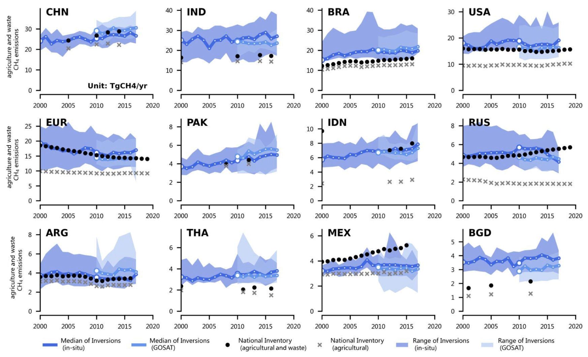
Figure 6CH4 emissions from agriculture and waste for the 12 largest emitters in this sector: China (CHN), India (IND), Brazil (BRA), the United States (USA), the EU27 and UK (EUR), Pakistan (PAK), Indonesia (IDN), Russia (RUS), Argentina (ARG), Thailand (THA), Mexico (MEX), and Bangladesh (BGD). The black dots denote the reported estimates from NGHGIs from the agriculture and waste sector, and the grey crosses denote NGHGI emissions from the agriculture sector only, the difference being the waste sector. Other lines, colors, and symbols are as in Fig. 4.
4.3 Agriculture and waste CH4 emissions
Figure 6 presents the CH4 emissions of the agriculture and waste sector for the top 12 emitters. Like in Fig. 5, the relative spread of inversions (min–max range divided by mean) is larger for this sector than for the total of all anthropogenic sectors. We observed that the median of GOSAT inversions is close to the median of in situ inversions within ±0.3 Tg CH4 yr−1 over the period 2009–2017 across the countries in Fig. 6. The values from NGHGIs also show good consistency with the inversions. In China (CHN), agriculture and waste emissions from the most recent NGHGI reports in the 2010s (28 Tg CH4 yr−1) are between the GOSAT inversions (29 Tg CH4 yr−1) and in situ inversions (27 Tg CH4 yr−1). The trend in agricultural emissions is consistent between inversions and NGHGIs for CHN. In India (IND), inversions give systematically higher emissions than NGHGIs by 50 % for GOSAT and 38 % for in situ inversions, with GOSAT and in situ inversions being similar in 2010 (∼24 Tg CH4 yr−1) and showing thereafter a decreasing trend in GOSAT (−0.1 Tg CH4 yr−1) compared to an increasing trend in in situ (+0.3 Tg CH4 yr−1) inversions. In IND, from the national inventory, enteric fermentation is the major CH4 source of the agriculture and waste sector, contributing 61 % of emissions with 20 % for rice cultivation and 16 % for waste. A similar result is found in Bangladesh (BGD), where agricultural emissions are dominated by rice production (48 % in 2012) and enteric fermentation (42 % in 2012), with GOSAT inversions giving emissions that are nearly double those of the NGHGI reports during 2001 and 2012. The large differences between the inversions and NGHGIs for IND and BGD could be due to the potential underestimation of livestock CH4 emissions by NGHGIs. NGHGIs used the Tier 1 method and associated emission factors from the 2006 IPCC Guidelines for National Greenhouse Gas Inventories (IPCC, 2006), while a recent study (Chang et al., 2021b) found that the estimates using the revised Tier 1 or Tier 2 methods from the 2019 Refinement to the 2006 IPCC Guidelines for National Greenhouse Gas Inventories (IPCC, 2019) are 48 %–60 % and 42 %–61 % higher for IND and BGD by 2010, respectively, and match better the inferred emissions from inversions. In Brazil (BRA), both GOSAT and in situ inversions are systematically larger than the NGHGIs by 34 % and by 29 %, respectively, but show a consistent increasing trend over their study periods. In the USA, the medians of GOSAT and in situ inversions are slightly higher than those of the NGHGIs, while NGHGIs show a slowly decreasing trend over the study period. In Indonesia (IDN), Pakistan (PAK), and Argentina (ARG), the medians of in situ inversions have a good consistency with NGHGI-reported values, while GOSAT inversion emissions in the 2010s are on average 19 % higher in Pakistan and 24 % higher in Argentina but 9 % lower in Indonesia compared to the NGHGI reports. In the EU27 and UK (EUR), emissions from agriculture and waste are found to have significantly decreased over time in the NGHGI data, mainly from solid waste disposal (Petrescu et al., 2021a), a trend that is captured by inversions and is close to the NGHGIs over the study period. In contrast, emissions from agriculture and waste in Russia (RUS) are reported to have a positive trend after 2010, contributed mainly by the solid waste disposal (crosses vs. circles in Fig. 6), whereas in situ inversions produce a consistent trend from 2000 to 2014 but a decrease thereafter, and the GOSAT inversions produce stable values, lower than the NGHGIs after 2010. Last, in Mexico (MEX), the inversion data in Fig. 6 indicate consistently lower agricultural and waste emissions than the NGHGIs, by 1.6 Tg CH4 yr−1 across in situ inversions and by 1.0 Tg CH4 yr−1 in the GOSAT inversions. Inversions produce stable emissions in the period after 2010, whereas the NGHGIs give an increase at a rate of 2 % yr−1, mainly from solid waste disposal (∼60 %) and livestock (∼40 %). Note that livestock CH4 emissions in Mexico increased by more than 20 % during 2000–2018 (from ∼2.0 to ∼2.4 Tg CH4 yr−1) from all methodologies used by Chang et al. (2021b) (2006 Tier 1, 2019 Tier 1, and Mixed Tier), suggesting that the increase in the national inventory agricultural emissions shown in Fig. 6 is consistent with more recent methodologies.
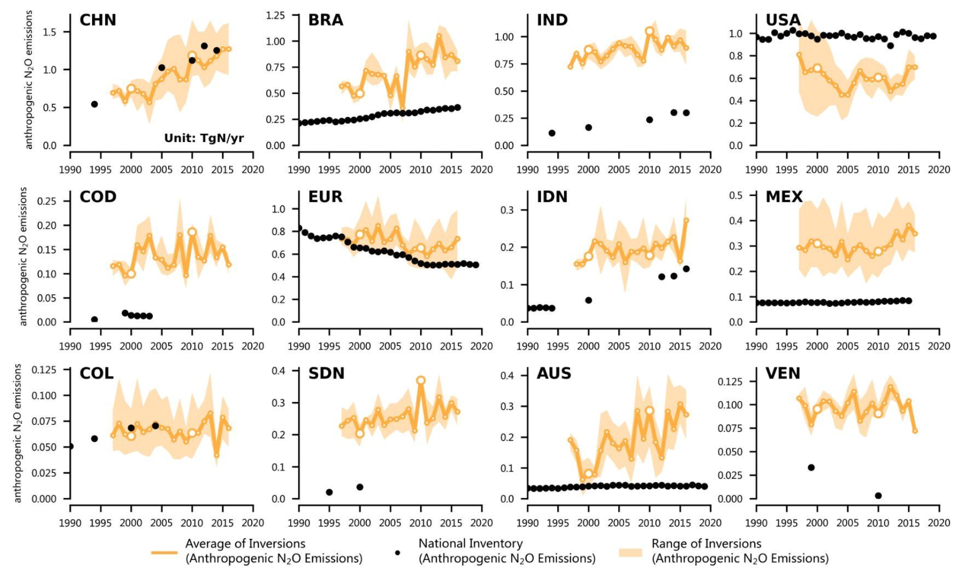
Figure 7Anthropogenic N2O fluxes of the top 12 emitters: China (CHN), Brazil (BRA), India (IND), the United States (USA), the Democratic Republic of the Congo (COD), the EU27 and UK (EUR), Indonesia (IDN), Mexico (MEX), Colombia (COL), Sudan (SDN), Australia (AUS), and Venezuela (VEN). The black dots denote the anthropogenic emissions from the UNFCCC national inventories. The thick orange lines denote the median of anthropogenic fluxes among N2O inversions, and the light orange areas denote the maximum–minimum ranges of all inversions. COD NC3 reports 2000–2010, but total emissions are inconsistent with sectoral emissions.
Figure 7 compares anthropogenic N2O emissions from inversions and NGHGIs. Inversions tend to produce higher emissions than NGHGIs, except for in the USA, China (CHN), and Colombia (COL). In all the countries considered, inversions show a larger interannual variability than NGHGI data. In the USA, the median of anthropogenic emissions from inversions is about 30 % lower than the inventories and shows a larger interannual variability with a minimum around the year 2005. In the EU27 and UK (EUR), the median of inversions became 32 % larger than NGHGIs after 2013, but inversions capture the decreasing trend of NGHGI-reported emissions before that year. This decreasing trend was attributed mainly to industrial emissions, according to NGHGI data and other inventories analyzed by Petrescu et al. (2021b). In general, the masking of unmanaged lands in gridded inversion fluxes reduces national emissions, in particular in tropical countries like the Democratic Republic of the Congo (COD) and Brazil (BRA), where unmanaged forests are significant emitters of N2O in inversions (see Fig. 12). Possible reasons for lower anthropogenic emissions for nearly all the non-Annex 1 countries can be the use of Tier 1 emission factors (EFs), which may be lower than when soil and climate dependence is accounted for (Philibert et al., 2013; Shcherbak et al., 2014; Q. Wang et al., 2020), and the non-linear observed concave response of cropland soil emissions as a function of added N fertilizers (Zhou et al., 2015), which makes emissions higher than the linear relation used by NGHGIs in Tier 1 approaches. In an ideal world, the EFs should represent the natural and anthropogenic components since these cannot be distinguished from field measurements, from which EFs are derived. In practice, the EFs are mostly based on measurements made in temperate climates and for soils of cropland established long ago with few “background” emissions. Therefore, there may be a systematic underestimation of default IPCC EFs from tropical climates, and recently established agricultural lands where the IPCC EFs also have huge uncertainty of up to ±75 %–100 %. Another reason may be the omission of emissions from reactive N contained in organic fertilizers (manure), about which NGHGIs do not provide details for non-Annex I reports. Last, anthropogenic indirect emissions (AIEs) from atmospheric nitrogen deposition and leaching of human-induced nitrogen additions to aquifers and inland waters are reported by Annex I countries using simple emission factors, but they are not systematically reported by non-Annex I countries. In Table S2, we compiled AIE data for the 20 highest N2O-emitting countries in the non-Annex I category, including the ones displayed in Fig. 7, using FAOSTAT data. Those indirect emissions represent 18 % of direct mineral-fertilizer-induced anthropogenic emissions from cropland soils in EUR and 16 % in the USA for instance and thus make NGHGI data systematically lower than inversions for countries that did not include them. According to the data in Table S2, indirect emissions represent 5 % to 10 % of anthropogenic emissions in most of the non-Annex I countries shown in Fig. 7. In consequence, their omission cannot explain the whole mismatch between NGHGIs and inversions. We also compared in Table S2 indirect emissions data from inventories with those provided by the FAOSTAT database (FAO, 2021).
In this section, we further analyze comparison between NGHGIs and inversions for the three gases. First, we compare the land CO2 flux to fossil fuel emissions and their respective trends. Then we discuss the uncertainty arising from the separation between anthropogenic and natural CH4 emissions in inversions by comparing the results of different separation methods, and we analyze how inversions resolve fossil versus agricultural emission budgets in each country. The contribution of CH4 emissions from ultra-emitters in the fossil fuel sector, which is not counted in inventories but could explain why inversions diagnose higher emissions than inventories in many oil- and gas-extracting countries, is further analyzed using independent estimates. Then, we analyze the separation of natural from anthropogenic sources in national N2O budgets from inversions, a topic which has not been addressed in previous studies. Finally, we compare the results of our global inversions with regional inversions based on higher-resolution transport models or assimilating regional data for China (CHN), the EU27 and UK (EUR), the USA, and Brazil (BRA).

Figure 8CO2 fluxes for land sinks and fossil emissions. Boxplots represent inversions for different time periods. Horizontal lines inside boxplots denote median values for inversions. Vertical lines of boxplots denote minimum and maximum values for selected time periods. Black horizontal lines symbolize net CO2 fluxes (fossil fuel and cement emissions + land flux) for inversions. Circumferences represent the mean of UNFCCC NGHGI data available for each time period.
6.1 Land CO2 fluxes compared to fossil fuel emissions
Figure 8 presents fossil fuel and cement emissions, the net land CO2 flux, and the net flux from the sum of the land flux and fossil emissions. Fossil CO2 emissions are obtained by re-aggregating to national totals the emission maps provided by each modeling group. These emissions are not optimized by inversions and may differ from UNFCCC NGHGIs because most non-Annex I countries do not have annual emission estimates and because inversions use as fixed priors gap-filled annual data from CDIAC and BP statistics for non-Annex I countries (Friedlingstein et al., 2020), whereas the red circles in Fig. 8 show the average of emissions from available BUR or NC reports in each period (thus, for each period only data of available years of national inventories are used to calculate the average). For Annex I countries, the prior fossil CO2 emission maps prescribed to the inversions from Jones et al. (2021) match by construction national totals from the UNFCCC. For non-Annex I countries, the prior fossil CO2 emission map is based mainly on CDIAC national emissions (Friedlingstein et al., 2020). The data presented in Fig. 8 show differences between NGHGI data and inversion priors, possibly due to (1) international bunker fuel emissions from ships and aviation counted in inversions as surface emissions but not included in UNFCCC national registers, (2) interpolation or regridding by inversion modelers of gridded fossil fuel emissions, or (3) our aggregation processing of national emissions from coarse-resolution inversions back to national totals (see Sect. 2.3). Residual differences have been corrected when presenting in Fig. 8 the land sink to match the emissions of Friedlingstein et al. (2020), but these inconsistencies of emissions between inventories and what is prescribed as prior fossil emissions in inversions should be kept in mind for future studies.
There is a striking consistency in Fig. 8 between means for each 6–7-year period of NGHGI land carbon sinks and inversions, after the adjustments presented in Sect. 2, for all major emitters. Although the range of inversions is large compared to the small uncertainties reported by NGHGI reports, the median value of inversions is within 37 % of NGHGIs for China (CHN), the USA, India (IND), and Brazil (BRA). Inversions give a larger sink compared to NGHGI data for several countries, however, such as Russia (RUS, by 85 %), the EU27 and UK (EUR, by 113 %), Australia (AUS, by >600 %), and Canada (CAN, >10 000 %). On the one hand, NGHGIs could potentially report lower estimation of carbon sinks in their managed lands due to incomplete estimation of environmental factors (e.g., CO2 fertilization effect) and incomplete reporting, especially for the soil pool (many of them assume that, e.g., mineral grassland soils are neutral, whereas this is probably not the case); however, the larger sink from inversions may also stem from prescribing bunker fuel aircraft emissions at the surface in the atmospheric transport models, which may imply a larger compensatory land CO2 sink. For CHN, given the large amount of fossil emissions, there is an aliasing effect between the choice of a prior emission estimate and the magnitude of the inferred national land sink (Saeki and Patra, 2017). For CAN and AUS, our proxy for unmanaged lands may explain systematically lower sink estimates in inventories compared to inversions. It should also be noted that Canada uses relatively old growth functions that do not capture much of the recent transient impact of environmental changes such as rising CO2 and longer growing seasons. AUS considers all forest as formally “managed”, but the vast majority (100 Mha of “other native forest”) is assumed to be in carbon equilibrium in the AUS NGHGIs. Thus with this assumption there is no biomass loss because the wood removal is zero, whereas old-growth forest may comprise carbon sinks.
In this study, we applied a mask of unmanaged forests to inversion gridded CO2 fluxes, which has mainly the effect of reducing CO2 uptake over the countries that have a large fraction of unmanaged forests, namely by 14 % in RUS, 30 % in CAN, 16 % in BRA, and 16 % in COD. BRA is a specific case because although large fractions of the Brazilian Amazon forest are slightly disturbed by “management” activities, it contains a significant fraction of protected areas and indigenous territories (23 % of the total forest area in BRA) (Alejo et al., 2021; IWGIA, 2021) which are counted as managed land by a political decision on land use. Thus, there is a large mismatch between nationally reported areas of unmanaged land (316 Mha in 2010 according to Table 3.109 from MCTI, 2016) and the intact forest mask that we used (166 Mha in 2010, ∼33 % of the national forest cover). According to Table 3 in the Supplement of Grassi et al. (2021), the share of total forest comprising intact forest was around 40 % in CAN and BRA and 20 % in RUS. This share depends on the threshold used to define forest, but in BRA, our intact forest area (16 %) used to exclude the inversion fluxes from unmanaged land seems to be too small. In comparison, the land carbon removals from NGHGIs are compiled based on the national communication reports of Brazil that say for instance that about half of Brazil's forest is unmanaged. We also note that we did nothing to mask unmanaged grasslands and rangelands for CO2 fluxes, even though these systems are thought to be larger CO2 sinks per unit area than managed grasslands (Chang et al., 2021a). In the future, it should be possible to mask inversions using the area simulated as managed grasslands by Chang et al. (2021a), that is, 1650 Mha or a fraction of 33 % of the global grassland area from their study. The masking of inversions' fluxes over unmanaged forests in the USA, CHN, and EUR has a negligible impact on the net land CO2 flux from inversions given their small/negligible share of forest being declared as unmanaged.
Regarding the effect of CO2 fluxes caused by lateral processes, which do not result in national carbon stock changes, the correction that we applied to inversions (Sect. 2) is equivalent to reproducing the rules of accounting by countries, where wood products harvested (also biofuels) are considered to be emitted where they have been produced, even though these products can be exported and CO2 emitted elsewhere. On the other hand, domestically produced and consumed wood, which comprises the majority of wood use in most countries, will induce subnational patterns of CO2 sources and sinks, assumed to be captured by inversions and not considered explicitly here as an inversion adjustment. To our knowledge, no country is accounting for carbon in traded crop products (as it is not a stock change) or for carbon transferred from soils to rivers and outgassed, buried in aquatic sediments, or transferred to the ocean. In inventories, observed soil carbon stock changes should implicitly include carbon leached or eroded from soils. However, since very few inventories are based on actual soil carbon change estimates but rather use assumptions or models that ignore the river loop of the carbon cycle, it is possible that the amount of carbon remaining in soils is overestimated by these approaches (Lauerwald et al., 2020). We found that altogether, the correction of inversions by CO2 fluxes induced by the lateral transport from river, crop, and wood products goes from a net source of 19 Tg C yr−1 in Sudan (mainly crop import) to a net sink of 169 Tg C yr−1 in Brazil (mainly lateral export). The river correction always makes the inversion net land CO2 flux a smaller sink, whereas the trade of crop and wood can be a net CO2 source or a sink, depending on the balance of exports and imports. We found that these trade fluxes are a source of CO2 in the net-importing countries China, the EU27 and UK, and Japan and a CO2 sink in wood- and food-exporting countries like the USA, Brazil, and Argentina. We outline the fact that most of the carbon lost by soils to rivers in a country is outgassed in territorial waters (see Sect. 2.3). Inversion results should partly include this source, although without prescribing it in an explicit manner (e.g., in their prior), but part of this CO2 source could also be misallocated to other countries in the flux increment of inversions. The same remark holds true for CO2 fluxes induced by crop and wood product growth, harvest, and trade. Although there is uncertainty about the share of unmanaged land as well as the lateral fluxes, we still make our efforts to narrow the gap between NGHGIs and inversions by excluding flues in unmanaged land and adjusting lateral fluxes from inversions. However, more profound and systematic analysis and comparisons are called for to harmonize the different scopes between national inventory compilations and inverse models.
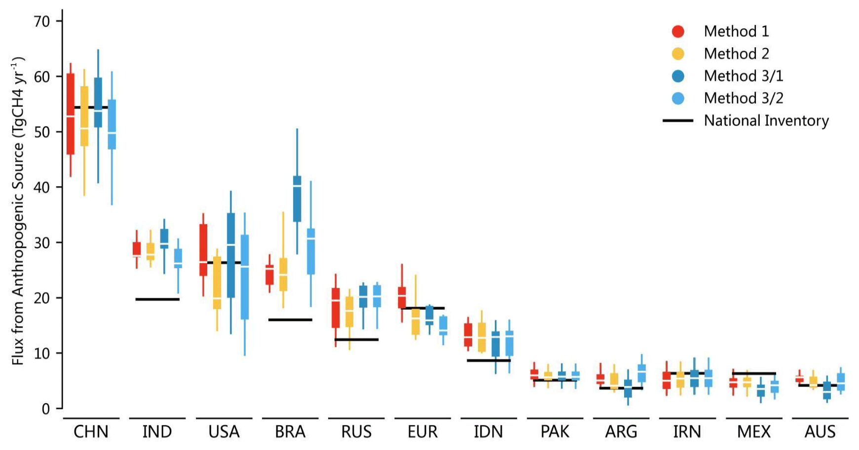
Figure 9Interquartile, min, and max of total anthropogenic CH4 emissions separated using different methods based on GOSAT inversions in the 2010s and the total anthropogenic CH4 emissions from NGHGIs. For each region, vertical boxes show the median, interquartile range, and min–max of the GOSAT inversions. Each color represents a different separation approach, as defined in Sect. 2.4. Black lines denote the average of total anthropogenic CH4 emissions from national inventories in the 2010s with available reported years.
6.2 Uncertainties due to the separation of natural from anthropogenic CH4 emissions
Uncertainty in anthropogenic CH4 emissions using the inversion method is suggested not only by the spread between models (due to transport models and other inversion specific settings) but also by the method chosen to separate anthropogenic from natural emissions. The data shown in Fig. 9 compare the results of the four different separation methods presented in Sect. 2. They show that the uncertainty due to the separation method is generally much smaller than the spread between different models, derived from the fact that inversion vertical ranges appear large relative to differences due to the separation procedure. In China (CHN), the between-method range of median inversion estimates of anthropogenic emissions is 4 Tg CH4 yr−1, compared to the mean model spread (interquartile) of 46–60 Tg CH4 yr−1. The range between the median of different methods is 10 Tg CH4 for the USA, 6 Tg CH4 for the EU27 and UK (EUR), and 3 Tg CH4 for Russia (RUS). In Brazil (BRA), methods 3/1 and 3/2 based on ecosystem models of wetland emissions to diagnose natural emissions give much larger anthropogenic emissions. This is likely because these models report lower natural emissions (Sawakuchi et al., 2014); e.g., they do not have emissions from flooded forests (Pangala et al., 2017), from the open river itself, or from palm swamps and peat complexes (Winton et al., 2017), which comprise an important CH4 source in BRA (Melack et al., 2004). Method 1, which is based on the original separation of natural vs. anthropogenic emissions from inversions, is not systematically different from other methods, but its results differ markedly due to its different use of data sources in each natural/anthropogenic part (see Sect. 2.4). Method 1 gives slightly higher anthropogenic emissions than other methods by 4 Tg CH4 yr−1 on average for EUR and by 3 Tg CH4 yr−1 for the USA and a smaller value than other methods by 1 Tg CH4 yr−1 for RUS. The positive difference between method 1, chosen for this study, and other methods (Fig. S5) implies a better match of inversions with respect to NGHGIs for EUR than if other methods were used. For the USA, if we were using method 2, the anthropogenic CH4 emissions would be smaller by 2 Tg CH4 yr−1, which would further accentuate lower estimations of inversion emissions compared to the NGHGIs, especially before 2010. For RUS, even if other methods were used to compare with NGHGIs, our result of a lower estimation of anthropogenic CH4 emissions by the NGHGI report remains valid. In CHN, our result that inversions produce systematically smaller anthropogenic CH4 emissions than NGHGI data is also robust to the choice of method.
Figure 10Total anthropogenic CH4 emissions from in situ (S) and GOSAT (G) inversions compared to NGHGIs (NI). S and G data correspond to the mean of inversion medians from the last 5 years of the available inversion data (2013 to 2017). Error bars denote minimum and maximum values for S and G inversions. NGHGI values represent the mean of the three most recent available country reports during the period 1999–2017. Dark red and black emissions represent the fraction of fossil fuel emissions from intensely emitting oil and gas (O&G) basins and from intensely emitting coal basins, respectively, derived from the Kayrros Methane Watch (Figs. S7 and S8, Table S3). On top of NGHGI emissions, emissions from ultra-emitters (red) are added to NGHGI estimates (diagnosed from S5P-TROPOMI measurements for the period 2019–2020; Lauvaux et al., 2022). For the countries where individual basin emissions are shown, the grey bar is the rest of the fossil emissions, i.e., the inversion fossil fuel emissions minus the sum of basins' emissions. Anthropogenic biomass burning was estimated by subtracting GFEDv4 emissions (van der Werf et al., 2017) excluding emissions over agricultural lands from the total biomass burning emissions of each inversion (method 1 in Sect. 2).
6.3 Contributions from fossil fuel versus agriculture and waste sectors in CH4 emissions
Figure 10 compares the share of the different sectors for anthropogenic CH4 emissions across a selection of 12 top emitting countries (selected countries from top anthropogenic and top fossil CH4 emitters). Generally, inversions partition agricultural and waste emissions consistently with NGHGIs within the respective uncertainties in both approaches. Inversions provide, however, larger biomass burning emissions than reported by NGHGIs, partly because we assumed that all biomass burning and biofuel emissions were anthropogenic in inversion results, whereas countries report only fire emissions on managed lands and emissions of biofuel burning used for house heating and cooking. Inversions tend to produce higher CH4 emissions than NGHGIs for all major oil- and gas-emitting countries (except CHN), in particular the USA, Russia (RUS), and Kazakhstan and Turkmenistan (KAZ&TKM). This under-reporting (also discussed in Sect. 4.2) can be due to the fact that inventories and emission factors do not consider CH4 leaks from ultra-emitting events consisting of very large and sporadic emissions, like accidental leaks (Cusworth et al., 2018). Here, we used the first global quantitative estimate of ultra-emitters derived by Lauvaux et al. (2022) from S5P-TROPOMI measurements, namely all short-duration leaks from oil and gas facilities (e.g., wells, compressors) with an individual emission >20 t CH4 h−1, with each event lasting generally less than 1 d. Using the event duration obtained by fitting a local dispersion model to observed S5P-TROPOMI methane plumes, all ultra-emitting events in each country were aggregated during the period from January 2019 to December 2020 (Table S3). Assuming that those large leaks are not reported by NGHGIs, they were added to NGHGI reports of fossil CH4 emissions as plain red stacked bars in Fig. 10. Doing so reduces the misfit with inversions, especially in RUS and KAZ&TKM. Ultra-emitters represent 85 % (1.4 Tg CH4 yr−1) of NGHGI fossil emissions for KAZ&TKM, 14 % (0.9 Tg CH4 yr−1) for RUS, and 2 % (0.03 Tg CH4 yr−1) for the countries grouped in the GULF region. We also considered emissions derived from S5P-TROPOMI measurements at the scale of regional extraction basins for oil, gas, and coal. Four major oil and gas basins were considered (Fig. S7) as they are specific areas where many individual wells and storage facilities are concentrated, each of them with a probability of emitting CH4 and forming a clear regional enhancement of CH4 detected in S5P-TROPOMI and imaged and assimilated with a regional inversion into a regional CH4 emission budget (see Table S3, Supplement, and Kayrros Methane Watch, https://www.kayrros.com/methane-watch/, last access: 30 July 2021). Such basin-scale emissions were diagnosed from regional inversions using S5P-TROPOMI atmospheric measurements. Here, we assumed that those basins are already counted as part of the national CH4 budgets from in situ and GOSAT inversions. Thus, they are shown here for the share of total national fossil emissions that they represent in inversions (dark red bars, part of total fossil emissions in inversion results displayed in Fig. 10). In the USA, the Permian basin emissions represent between 21 % (in situ, S) and 24 % (GOSAT, G) of the total national fossil CH4 estimates from inversions. Alone, the Permian basin contributed 16 % of the total gas and 35 % of the oil extracted in the USA in 2019 (EIA, 2021a). Our average 2019–2020 emission estimate in the Permian basin is 2.3 Tg CH4 yr−1 from S5P-TROPOMI data, which is consistent with an estimate of 2.7 Tg CH4 yr−1 from O&G industries in the Permian basin reported by Zhang et al. (2020) but contrasts with the 1.4 Tg CH4 yr−1 emission estimate for the entire USA reported by EPA (2020). In the GULF, emissions from the basin comprising Iraq and Kuwait represent 32 % (S)–46 % (G) of the total estimated fossil emissions of this region. This basin estimation encompasses four of the highest-oil-producing fields in the world, and its oil production accounts for 31.5 % of all the countries in the GULF region (EIA, 2021a). The basin estimation from inversions for IRN (2.3 Tg CH4) represents 55.2 % (S)–71.0 % (G) of estimated fossil fuel emissions and 94.8 % of the national total NGHGI estimates.

Figure 11N2O emission fluxes in Tg N yr−1 for CAMS (C), GEOS-Chem (G), and INVICAT (T) inversions compared to NGHGI (NI) data for 2010–2016. C, G, and T data correspond to the mean of fluxes from 2010 to 2016. NGHGI values represent the mean of available data for the same period. Anthropogenic river emissions are from Yao et al. (2019), and they are represented for information as part of managed land emissions, as they are captured by inversions (Sect. 2). Natural river emissions are considered the average of 1900–1910 (Sect. 2) and are removed from total emissions of inversions. Data of wildfires correspond to GFEDv4-reported values for the period of interest (van der Werf et al., 2017). They are counted as non-anthropogenic emissions following Eq. (6) in Sect. 2 and reported here for information.
6.4 Overlooked importance of natural N2O emissions in non-Annex I countries
As shown in Sect. 5, the estimation of N2O emission fluxes by emission inventories is challenging, and currently some non-Annex I countries (e.g., COD) have no estimates available. Figure 11 compares inversions (CAMS, GEOS-Chem, and INVICAT) to available NGHGI-reported N2O emission fluxes. Because emission sectors of NGHGIs and inversions are limited and do not coincide with each other, the comparison of N2O emission sectors between these two data sources can only be accomplished partially. The main innovation proposed in this study has been to separate total inversion fluxes into unmanaged and managed lands so that the emissions over managed lands minus the natural inland water emissions can be compared with inventories (Sect. 2). We can see in the data presented in Fig. 12 that natural emissions (natural fluxes from lakes and rivers plus fluxes from unmanaged lands) account for 32 % of the mean inversion total in BRA, 47 % in COD, and 57 % in AUS. In temperate industrialized countries with a smaller fraction of unmanaged land, the magnitude of natural fluxes relative to anthropogenic ones is smaller. In comparison to emissions from unmanaged lands, the natural emissions from rivers are always of a very small magnitude. In general, removing natural emissions tends to improve the agreement with inventories in non-Annex I countries. In Annex I countries, it tends to make inversion-based emissions smaller than those of NGHGIs. The main uncertainty is in the area of grasslands and forests assumed to be unmanaged from our masks and how well they correspond to the unmanaged areas used by each country. A large area of extensively grazed land, e.g., in Mongolia and Kazakhstan, is considered here natural, whereas those countries may consider them under management, even though the nitrogen cycle and N2O emissions are close to natural conditions for extensive grazing. The consistent pattern of higher emissions in inversions than NGHGIs among the three model inversions for non-Annex I countries suggests possible improvements in inventory compilation including adopting country-specific emission factors or re-assessing and reporting indirect emissions when this is not the case (Table S2). On the other hand, for the USA and CHN, the median of inversion emissions is smaller than in inventories and CAMS is higher than the two other inversions considered. Concerning smaller inversion estimates for CHN and the USA compared to NGHGIs, this could be because the Tier 1 used by NGHGIs assumes static EFs, whereas EFs may change (become smaller or larger) depending on cropland nitrogen use efficiency (NUE) and climate. The USA improved its NUE in the 1990s compared to the 1980s considerably (Lassaletta et al., 2014), but if the EFs used are based on flux measurements in the 1980s, these could be too high. A recent data-driven model of direct cropland N2O emissions (Q. Wang et al., 2020) using non-linear EF and regional N-fertilizer input data found emissions smaller than those found by Tier 1 methods, which would be in better agreement with inversions. Another source of uncertainty in the N2O inversions is the prior estimates for land versus ocean. Since the ocean is not well constrained in the inversions, having a too high ocean prior will mean the land total will be underestimated and vice versa.
6.5 Comparison with regional emissions
Table 3 compares the results of the global inversions used in this study with regional inversion results compiled from the literature, generally obtained with higher-resolution regional transport models and sometimes using atmospheric data not assimilated by global inversions. Global inversion results are given without and with adjustments for CO2 fluxes due to lateral transport and for anthropogenic emissions estimated using equation method 1 for CH4 and Eq. (6) for N2O (Sect. 2). The purpose of introducing a CO2 flux correction (Sect. 2.3) was to make an accurate comparison with inventories, but since regional CO2 inversions did not use such an adjustment, here we focus on comparing regional inversions with global ones without adjustment.
For CO2 fluxes in CHN, except for the large uptake found by the inversion (J. Wang et al., 2020), all previous regional inversion results fall within the range of our global inversion ensemble for their period of overlap, indicating no systematic bias of global inversions. Note that J. Wang et al. (2020) provide a global inversion using new Chinese stations data and a discretization of fluxes into smaller sub-regions within China. In BRA, the range of global inversions also covers regional inversion results yet with global inversions being a small CO2 source in 2010 (194 Tg C yr−1) and regional inversions a large source in that year. The regional inversions from Gatti et al. (2014) and Van der Laan-Luijkx et al. (2015) using aircraft CO2 and CO profiles in the Amazon also give a larger flux change between 2010 (a dry year, a CO2 source in the Amazon) and 2011 (a wet year, a CO2 sink in the Amazon) than global inversions that do not assimilate these aircraft data. For EUR, the range of regional inversions (Petrescu et al., 2021a) is similar to the one of global inversions. For North America, however, regional inversions give a higher average CO2 uptake than global ones, although within their range.
For CH4 emissions in CHN, the results of all regional inversions (Miller et al., 2019; Thompson et al., 2015) are consistent with our global inversion ensemble, although the inversion of Miller et al. (2019) is in the upper range. For BRA or the Amazon basin, interestingly, regional inversions (Tunnicliffe et al., 2020; Wilson et al., 2016) provide systematically higher CH4 emissions than global in situ inversion estimates, but regional inversions include wetlands and rivers, which can explain their higher values. If natural emissions were removed from regional inversions, then their values would be consistent with global results; i.e., Tunnicliffe et al. (2020) estimated that CH4 emissions from BRA are 33.6±3.6 Tg CH4 yr−1 with 19.0±2.6 Tg CH4 yr−1 from anthropogenic sources, falling within the range of our estimates for anthropogenic emissions from global inversions (19–36 Tg CH4 yr−1). In the EU and the USA or North America, the regional inversions in Table 3 which have higher-resolution transport models give higher CH4 emissions than global inversions, even when only anthropogenic emissions are considered in regional inversions. This suggests that global models may systematically underestimate CH4 emissions from those two high emitters. For N2O, we have several regional inversions for North America, all producing higher emissions than the median of global inversions by a factor of 4, on average. The only regional N2O inversion over Europe is also about 2 times higher than the median of global inversions.
Table 3Comparison of global inversions in this study with regional inversions from the literature (the range from the inversion ensemble is given in parentheses, unless stated otherwise). Values in bold text are statistically valid in that the regional inversion results fall within the range of our global inversion ensemble.
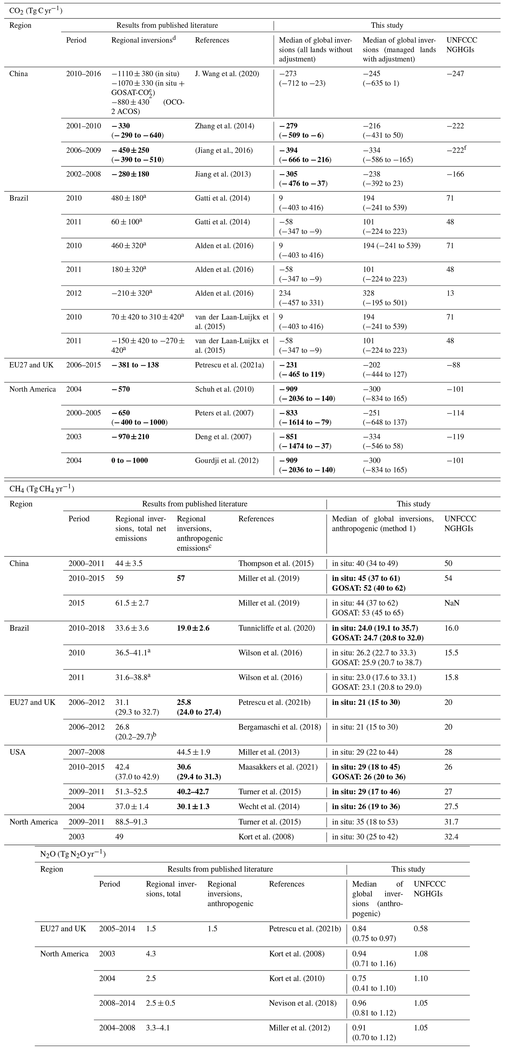
a Estimates for the Amazon Basin. b The 10th and 90th percentiles. c The separation of anthropogenic emissions from regional emissions excludes wetlands but uses different methods than in this study. d No adjustment of regional CO2 inversion results was performed, unlike in column 5 and based on Eq. (1) for global inversions. e GOSAT ACOS and OCO-2 ACOS XCO2 products (Kong et al., 2019; GES DISC, 2021). f For China, only two NGHGI reports are available, in 2005 and 2010, and the average of the two years is given in the table.
GHG (CO2, CH4, N2O) data from inverse models and UNFCCC national inventories are available at https://doi.org/10.5281/zenodo.5089799 (Deng et al., 2021).
This dataset contains five data files, including GHG data from inverse models and UNFCCC national inventories in the top emitter countries.
- –
CO2_inversion_1990-2019. This contains annual CO2 flux data from 6 inversion models in three sectors:
- •
-
“land flux (all land)”, i.e., land flux from all land;
- •
-
“land flux (managed land)”, i.e., land flux from managed land;
- •
-
“land flux (managed land + lateral adjustment)”, i.e., land flux from managed land by adjusting the lateral flux.
- –
CH4_inversion_2000-2017. This contains CH4 flux data from 10 in situ inversion (2000–2017) and 11 satellite inversion (2010–2017) models from four sectors:
- •
-
“anthropogenic (method x)”, i.e., anthropogenic emissions from managed land, where x could be 1, 2, 3/1, or 3/2, representing different methods to calculate the emissions in this sector;
- •
-
“fossil”, i.e., emissions from the fossil sector;
- •
-
“agriculture & waste”, i.e., emissions from the agriculture and waste sector combined;
- •
-
“biomass burning”, i.e., emissions from biomass burning.
- –
N2O_inversion_1997-2016. This contains anthropogenic N2O emissions data from 3 models.
- –
Inventory_1990-2019. This contains inventory data collected from UNFCCC national inventories. The classification of sectors corresponds with the inversion data files for each gas species.
- –
Inventory_1990-2019_IPCC. This contains inventory data collected from UNFCCC national inventories in the IPCC category.
This study proposes a new toolbox to improve the consistency between inversions and UNFCCC NGHGIs for each of the three greenhouse gases. We post-processed inversion results to make them comparable with the rules of accounting of inventories. For CO2, we excluded the fluxes in unmanaged lands with an intact forest mask and estimated the fluxes associated with lateral transport (by river or by trade). For CH4, we proposed three methods to split the anthropogenic fluxes from inversions by aggregating prior estimates from each sector or by removing fluxes of natural processes. For N2O, we also separated the fluxes from managed land by using the same method on CO2 and accounting for the indirect N2O emissions. In the case of CO2, using a mask of managed lands is also critical for large forested countries (Grassi et al., 2021) and tends to make their “carbon sink” smaller than when using inversion fluxes over all the grid cells. Here we made a first attempt to use an intact “non-managed” forest mask for this purpose. Such a mask could be extended to unmanaged grasslands in future studies, e.g., following recent work by Chang et al. (2021a). However, it should be noted that there are discrepancies between the intact forest landscape maps of Potapov et al. (2017) that we use and the unmanaged land defined in NGHGIs. For instance, an intact forest protected in a national park will be classified as managed in the corresponding NIR. Conversely, some areas of “unmanaged forest” are outside of the intact forests defined by Potapov et al. (2017), e.g., northern open woodlands. Here, we recommend that countries should report their managed land in a spatially explicit manner to enable a better evaluation of national emissions reports using inversions (and other observation-based approaches), and countries should also follow the recommendations of the IPCC 2006 guidelines encouraging countries to use atmospheric data as an independent check on their national reports (IPCC, 2006, 2019) (see also the discussion in Chevallier, 2021). Removing from inversions the CO2 fluxes coupled to lateral transport, which represent no carbon stock change and are not all visible to inventories, generally makes the carbon sink significantly smaller in northern mid-latitude countries (e.g., 26 % in CAN and 18 % lower in RUS) than if raw inversion data were used. All harvest is seen by NGHGIs as a loss of carbon stock in forest. Then, the wood that remains in the country enters the harvested wood products (HWP) pool (where gains and losses are recorded). What is “invisible” in NGHGIs is the wood that enters the HWP pool of a foreign country. CH4 and N2O emissions have been even less explored for a systematic comparison of inversions with inventories. For these two gas species, we improved the processing of inversion gridded fluxes to separate anthropogenic fluxes from the total emissions in order to provide estimates that can be compared with NGHGIs for policy implementation. For CH4, we proposed three methods to remove the signal of natural CH4 emissions and found that their robustness is country dependent, the separation of natural emissions to retrieve anthropogenic emissions being more difficult in countries that have both large natural and anthropogenic emissions and few atmospheric stations, like RUS or BRA. We certainly recommend here to reduce the uncertainty in prior estimates and improve estimations of natural sources using, e.g., better bottom-up datasets of wetland area, rivers, and lakes and their CH4 emissions rates in order to make further in-depth comparisons between these methods. For CH4, a second notable result is that despite the large spread of inversions, both in situ and GOSAT inversions show valid differences from NGHGI anthropogenic emissions. We also found that Kazakhstan and Turkmenistan in central Asia and the Gulf countries in the Middle East, characterized by oil- and gas-producing industries, report much lower CH4 emissions than atmospheric inversions. It is fair to say that in this region, there are few ground stations, and inversions could depend on their prior fluxes, but the fact that GOSAT and in situ data point to NGHGI emissions being underestimated suggests areas for future research to constrain the emissions of these countries. We recommend here developing regional campaigns (such as those performed in Alvarez et al., 2018) to refine emission factors and to track regional oil, gas, and coal basin emissions and ultra-emitter site level emissions using new tools (such as moderate- and high-resolution satellite imagery). For N2O, the prevalence of large tropical natural sources, being outside the responsibility of countries if they are located on unmanaged lands, has been overlooked before. For example, nearly half of the forests in Brazil are unmanaged according to its national inventory report. We did not solve this problem but highlighted it and proposed a new method to remove natural emissions from inversion total emissions. As many non-Annex I countries which will have to produce inventories for the global stocktake are tropical countries with a very active nitrogen cycle and large natural N2O emissions, a decoupling will exist between targeted emissions reductions and the observed growth rate of N2O; it may hamper the eventual effectiveness of mitigation policies that are directly reflected in the UNFCCC NGHGI reports, especially for this greenhouse gas.
It is fair to say that the uncertainty from inversions from the spread of different models is generally large, so inversions cannot “falsify” NGHGIs in most instances. Nevertheless, for CH4 in countries around the Persian Gulf and central Asia and to some extent in Russia and for N2O in tropical countries, Mexico, and Australia, we found that NGHGI emissions are significantly lower than inversions, which suggests that activity data or emission factors may need to be re-evaluated. Despite their large spread, inversions have the advantage of providing fluxes that are consistent with the accurately observed growth rates of each greenhouse gas in the atmosphere. The uncertainty in inversions is mainly a systematic bias due to internal settings or to the choice of a transport model. It does not mean that inversions cannot be used for monitoring interannual variability and trends of fluxes, in response to mitigation efforts, since most of their bias should have a small temporal component.
The study of global inversions at the country scale rather than at the traditional subcontinent scale (e.g., the “TransCom 3 regions” of Gurney et al., 2002) obviously pushes inversions close to the limit of their domain of validity, even in the case of large countries. The densification of observation networks and systems, especially from space, increases the observational information available at all spatial scales and gradually makes it possible to study smaller countries. This densification must be accompanied by a corresponding increase in the horizontal resolution of inversion systems (both the transport model and the control vector to be optimized). Note that the spatial resolution of most inverse models such as those contributing to the global carbon–methane–nitrous oxide budget is larger than 1∘ (see Table A4 in Friedlingstein et al., 2020; Table S6 in Saunois et al., 2020; and Table 18 in the Supplement of Tian et al., 2020). They will likely soon have to go below 1∘ on a global scale to remain competitive for this type of study, despite the high computational challenge posed by the atmospheric inversion of long-lived tracers.
The supplement related to this article is available online at: https://doi.org/10.5194/essd-14-1639-2022-supplement.
ZD, PC, MS, and FC designed and coordinated the study. PC, MS, CQ, RLT, HT, YH, and FC designed the framework of atmosphere inversion data processing. ZD, PC, ZATS, MS, CQ, and FC performed the post-processing and analysis and wrote the paper. ZD, CT, TS, PK, and YC compiled the national greenhouse gas inventories. MS, RLT, HT, and FC gathered the global atmosphere inversion datasets of CO2, CH4, and N2O. HT and YY provided the inland water N2O emissions. CQ and RL provided the lake CH4 emissions. CQ processed and provided the downscaled geological CH4 emissions and conducted the comparison with regional inversions. XX provided the CO2 flux embodied in food trade. TL, AdA, CG, and ABe provided the CH4 emissions from ultra-emitters. JC provided the lightly grazed grassland mask. FC processed the atmosphere inversion data with masks of intact forest, lightly grazed grassland, and country boundaries. ZD, PC, ZATS, TL, and FC produced the figures. ZD, PC, ZATS, MS, CQ, KT, XL, RLT, HT, YY, YH, RL, AKJ, XX, ABa, SS, PIP, TL, AdA, CG, ABe, BP, JC, AMRP, SJD, ZL, GG, CA, FNT, LP, WP, and FC contributed to the updating of the full text and appended comments.
The contact author has declared that neither they nor their co-authors have any competing interests.
Publisher's note: Copernicus Publications remains neutral with regard to jurisdictional claims in published maps and institutional affiliations.
The authors are very grateful to the atmosphere inversion model developers Aki Tsuruta, Arjo Segers, Bo Zheng, Chris Wilson, Christian Rödenbeck, Kelley Wells, Liesbeth Florentie, Misa Ishizawa, Naveen Chandra, Peter Bergamaschi, Prabir Patra, Shamil Maksyutov, Yi Yin, and Yosuke Niwa for the availability of their global CO2, CH4, and N2O inversion data and acknowledge many other data providers (measurements, models, inventories, atmospheric inversions, hybrid products, etc.) that are directly or indirectly used in this synthesis.
This research has been supported by the European Space Agency Climate Change Initiative (ESA CCI) RECCAP2 project (grant no. ESRIN/4000123002/18/I-NB) and by the European Commission Prototype system for a Copernicus CO2 service (CoCO2, grant no. 958927); the “Investissements d'avenir” program, reference ANR-19-P3IA-0001 (PRAIRIE 3IA Institute); and the Observation-based system for monitoring and verification of greenhouse gases (VERIFY, grant no. 725546).
This paper was edited by David Carlson and reviewed by two anonymous referees.
Alden, C. B., Miller, J. B., Gatti, L. V., Gloor, M. M., Guan, K., Michalak, A. M., van der Laan-Luijkx, I. T., Touma, D., Andrews, A., Basso, L. S., Correia, C. S. C., Domingues, L. G., Joiner, J., Krol, M. C., Lyapustin, A. I., Peters, W., Shiga, Y. P., Thoning, K., van der Velde, I. R., van Leeuwen, T. T., Yadav, V., and Diffenbaugh, N. S.: Regional atmospheric CO2 inversion reveals seasonal and geographic differences in Amazon net biome exchange, Glob. Chang. Biol., 22, 3427–3443, https://doi.org/10.1111/gcb.13305, 2016.
Alejo, C., Meyer, C., Walker, W. S., Gorelik, S. R., Josse, C., Aragon-Osejo, J. L., Rios, S., Augusto, C., Llanos, A., Coomes, O. T., and Potvin, C.: Are indigenous territories effective natural climate solutions? A neotropical analysis using matching methods and geographic discontinuity designs, PLoS One, 16, e0245110, https://doi.org/10.1371/journal.pone.0245110, 2021.
Allen, D. T.: Emissions from oil and gas operations in the United States and their air quality implications, J. Air Waste Manag. Assoc., 66, 549–575, https://doi.org/10.1080/10962247.2016.1171263, 2016.
Alvarez, R. A., Zavala-Araiza, D., Lyon, D. R., Allen, D. T., Barkley, Z. R., Brandt, A. R., Davis, K. J., Herndon, S. C., Jacob, D. J., Karion, A., Kort, E. A., Lamb, B. K., Lauvaux, T., Maasakkers, J. D., Marchese, A. J., Omara, M., Pacala, S. W., Peischl, J., Robinson, A. L., Shepson, P. B., Sweeney, C., Townsend-Small, A., Wofsy, S. C., and Hamburg, S. P.: Assessment of methane emissions from the U.S. oil and gas supply chain, Science, 361, 186–188, https://doi.org/10.1126%2Fscience.aar7204, 2018.
Aragão, L. E. O. C., Anderson, L. O., Fonseca, M. G., Rosan, T. M., Vedovato, L. B., Wagner, F. H., Silva, C. V. J., Silva Junior, C. H. L., Arai, E., Aguiar, A. P., Barlow, J., Berenguer, E., Deeter, M. N., Domingues, L. G., Gatti, L., Gloor, M., Malhi, Y., Marengo, J. A., Miller, J. B., Phillips, O. L., and Saatchi, S.: 21st Century drought-related fires counteract the decline of Amazon deforestation carbon emissions, Nat. Commun., 9, 536, https://doi.org/10.1038/s41467-017-02771-y, 2018.
Balsamo, G., Engelen, R., Thiemert, D., Agusti-Panareda, A., Bousserez, N., Broquet, G., Brunner, D., Buchwitz, M., Chevallier, F., Choulga, M., Denier Van Der Gon, H., Florentie, L., Haussaire, J.-M., Janssens-Maenhout, G., Jones, M. W., Kaminski, T., Krol, M., Le Quéré, C., Marshall, J., McNorton, J., Prunet, P., Reuter, M., Peters, W., and Scholze, M.: The CO2 Human Emissions (CHE) Project: First Steps Towards a European Operational Capacity to Monitor Anthropogenic CO2 Emissions, Front. Remote Sens., 2, 707247, https://doi.org/10.3389/frsen.2021.707247, 2021.
Bastos, A., Fu, Z., Ciais, P., Friedlingstein, P., Sitch, S., Pongratz, J., Weber, U., Reichstein, M., Anthoni, P., Arneth, A., Haverd, V., Jain, A., Joetzjer, E., Knauer, J., Lienert, S., Loughran, T., McGuire, P. C., Obermeier, W., Padrón, R. S., Shi, H., Tian, H., Viovy, N., and Zaehle, S.: Impacts of extreme summers on European ecosystems: a comparative analysis of 2003, 2010 and 2018, Philos. T. R. Soc. Lond. B, 375, 20190507, https://doi.org/10.1098/rstb.2019.0507, 2020.
Bergamaschi, P., Karstens, U., Manning, A. J., Saunois, M., Tsuruta, A., Berchet, A., Vermeulen, A. T., Arnold, T., Janssens-Maenhout, G., Hammer, S., Levin, I., Schmidt, M., Ramonet, M., Lopez, M., Lavric, J., Aalto, T., Chen, H., Feist, D. G., Gerbig, C., Haszpra, L., Hermansen, O., Manca, G., Moncrieff, J., Meinhardt, F., Necki, J., Galkowski, M., O'Doherty, S., Paramonova, N., Scheeren, H. A., Steinbacher, M., and Dlugokencky, E.: Inverse modelling of European CH4 emissions during 2006–2012 using different inverse models and reassessed atmospheric observations, Atmos. Chem. Phys., 18, 901–920, https://doi.org/10.5194/acp-18-901-2018, 2018.
Brown, P., Broomfield, M., Cardenas, L., Choudrie, S., Jones, L., Karagianni, E., Passant, N., Thistlethwaite, G., Thomson, A., Turtle, L., and Others: UK Greenhouse Gas Inventory, 1990 to 2019: Annual Report for submission under the Framework Convention on Climate Change, Department for Business, Energy & Industrial Strategy, ISBN 978-0-9933975-7-8, 2021.
Bullock, E. L., Woodcock, C. E., Souza Jr., C., and Olofsson, P.: Satellite-based estimates reveal widespread forest degradation in the Amazon, Glob. Chang. Biol., 26, 2956–2969, https://doi.org/10.1111/gcb.15029, 2020.
Canadell, J., Ciais, P., Sabine, C., and Joos, F. (Eds.): REgional Carbon Cycle Assessment and Processes (RECCAP), Biogeosciences, https://bg.copernicus.org/articles/special_issue107.html (last access: 5 December 2021), 2012.
Chandra, N., Patra, P. K., Bisht, J. S. H., Ito, A., Umezawa, T., Saigusa, N., Morimoto, S., Aoki, S., Janssens-Maenhout, G., Fujita, R., Takigawa, M., Watanabe, S., Saitoh, N., and Canadell, J. G.: Emissions from the Oil and Gas Sectors, Coal Mining and Ruminant Farming Drive Methane Growth over the Past Three Decades, J. Meteorol. Soc. Japan. Ser. II, 99, 309–337, https://doi.org/10.2151/jmsj.2021-015, 2021.
Chang, J., Ciais, P., Gasser, T., Smith, P., Herrero, M., Havlík, P., Obersteiner, M., Guenet, B., Goll, D. S., Li, W., Naipal, V., Peng, S., Qiu, C., Tian, H., Viovy, N., Yue, C., and Zhu, D.: Climate warming from managed grasslands cancels the cooling effect of carbon sinks in sparsely grazed and natural grasslands, Nat. Commun., 12, 118, https://doi.org/10.1038/s41467-020-20406-7, 2021a.
Chang, J., Peng, S., Yin, Y., Ciais, P., Havlik, P., and Herrero, M.: The key role of production efficiency changes in livestock methane emission mitigation, AGU Advances, 2, e2021AV000391, https://doi.org/10.1029/2021av000391, 2021b.
Chevallier, F.: Fluxes of carbon dioxide from managed ecosystems estimated by national inventories compared to atmospheric inverse modeling, Geophys. Res. Lett., 48, e2021GL093565, https://doi.org/10.1029/2021gl093565, 2021.
Chevallier, F., Fisher, M., Peylin, P., Serrar, S., Bousquet, P., Bréon, F.-M., Chédin, A., and Ciais, P.: Inferring CO2 sources and sinks from satellite observations: Method and application to TOVS data, J. Geophys. Res., 110, D24309, https://doi.org/10.1029/2005jd006390, 2005.
Ciais, P., Reichstein, M., Viovy, N., Granier, A., Ogée, J., Allard, V., Aubinet, M., Buchmann, N., Bernhofer, C., Carrara, A., Chevallier, F., De Noblet, N., Friend, A. D., Friedlingstein, P., Grünwald, T., Heinesch, B., Keronen, P., Knohl, A., Krinner, G., Loustau, D., Manca, G., Matteucci, G., Miglietta, F., Ourcival, J. M., Papale, D., Pilegaard, K., Rambal, S., Seufert, G., Soussana, J. F., Sanz, M. J., Schulze, E. D., Vesala, T., and Valentini, R.: Europe-wide reduction in primary productivity caused by the heat and drought in 2003, Nature, 437, 529–533, https://doi.org/10.1038/nature03972, 2005.
Ciais, P., Yao, Y., Gasser, T., Baccini, A., Wang, Y., Lauerwald, R., Peng, S., Bastos, A., Li, W., Raymond, P. A., Canadell, J. G., Peters, G. P., Andres, R. J., Chang, J., Yue, C., Dolman, A. J., Haverd, V., Hartmann, J., Laruelle, G., Konings, A. G., King, A. W., Liu, Y., Luyssaert, S., Maignan, F., Patra, P. K., Pere- gon, A., Regnier, P., Pongratz, J., Poulter, B., Shvidenko, A., Valentini, R., Wang, R., Broquet, G., Yin, Y., Zscheischler, J., Guenet, B., Goll, D. S., Ballantyne, A.-P., Yang, H., Qiu, C., and Zhu, D.: Empirical estimates of regional carbon budgets imply reduced global soil heterotrophic respiration, Natl. Sci. Rev., 8, nwaa145, https://doi.org/10.1093/nsr/nwaa145, 2020.
Ciais, P., Bastos, A., Chevallier, F., Lauerwald, R., Poulter, B., Canadell, J. G., Hugelius, G., Jackson, R. B., Jain, A., Jones, M., Kondo, M., Luijkx, I. T., Patra, P. K., Peters, W., Pongratz, J., Petrescu, A. M. R., Piao, S., Qiu, C., Von Randow, C., Regnier, P., Saunois, M., Scholes, R., Shvidenko, A., Tian, H., Yang, H., Wang, X., and Zheng, B.: Definitions and methods to estimate regional land carbon fluxes for the second phase of the REgional Carbon Cycle Assessment and Processes Project (RECCAP-2), Geosci. Model Dev., 15, 1289–1316, https://doi.org/10.5194/gmd-15-1289-2022, 2022.
Copernicus: OBSERVER: Monitoring Anthropogenic CO2 emissions with Copernicus, https://www.copernicus.eu/en/news/news/observer-monitoring-anthropogenic-co2-emissions-copernicus, last access: 2 July 2021.
Crowell, S., Baker, D., Schuh, A., Basu, S., Jacobson, A. R., Chevallier, F., Liu, J., Deng, F., Feng, L., McKain, K., Chatterjee, A., Miller, J. B., Stephens, B. B., Eldering, A., Crisp, D., Schimel, D., Nassar, R., O'Dell, C. W., Oda, T., Sweeney, C., Palmer, P. I., and Jones, D. B. A.: The 2015–2016 carbon cycle as seen from OCO-2 and the global in situ network, Atmos. Chem. Phys., 19, 9797–9831, https://doi.org/10.5194/acp-19-9797-2019, 2019.
Cusworth, D. H., Jacob, D. J., Sheng, J.-X., Benmergui, J., Turner, A. J., Brandman, J., White, L., and Randles, C. A.: Detecting high-emitting methane sources in oil/gas fields using satellite observations, Atmos. Chem. Phys., 18, 16885–16896, https://doi.org/10.5194/acp-18-16885-2018, 2018.
Davis, K. F., Yu, K., Rulli, M. C., Pichdara, L., and D'Odorico, P.: Accelerated deforestation driven by large-scale land acquisitions in Cambodia, Nat. Geosci., 8, 772–775, https://doi.org/10.1038/ngeo2540, 2015.
Deng, F., Chen, J. M., Ishizawa, M., Yuen, C.-W., Mo, G., Higuchi, K., Chan, D., and Maksyutov, S.: Global monthly CO2 flux inversion with a focus over North America, Tellus B, 59, 179–190, https://doi.org/10.1111/j.1600-0889.2006.00235.x, 2007.
Deng, Z., Ciais, P., Tzompa-Sosa, Z., Saunois, M., Chevallier, F., Tan, C., Sun, T., Ke, P., Cui, Y., and Liu, Z.: GHG data from inverse models and UNFCCC national inventories v0.1, Zenodo [data set], https://doi.org/10.5281/zenodo.5089799, 2021.
DISER: National Inventory Report 2019, Department of Industry, Science, Energy and Resources, https://unfccc.int/documents/273478 (last access: 4 April 2022), 2021.
EIA: Drilling productivity report, U.S. Energy Information Administration, https://www.eia.gov/petroleum/drilling/, last access: 7 July 2021a.
EIA: U.S. natural gas gross withdrawals and production, https://www.eia.gov/dnav/ng/ng_prod_sum_dc_NUS_mmcf_a.htm, last access: 7 July 2021b.
EIA: Where our natural gas comes from, https://www.eia.gov/energyexplained/natural-gas/where-our-natural-gas-comes-from.php, last access: 7 July 2021c.
EPA: Inventory of U.S. Greenhouse Gas Emissions and Sinks: 1990–2018, United States Environmental Protection Agency, EPA 430-R-20-002, 2020.
Etiope, G., Ciotoli, G., Schwietzke, S., and Schoell, M.: Gridded maps of geological methane emissions and their isotopic signature, Earth Syst. Sci. Data, 11, 1–22, https://doi.org/10.5194/essd-11-1-2019, 2019.
FAO: FAOSTAT Emissions Totals, FAO, Rome, https://www.fao.org/faostat/en/?#data/GT, last access: 7 July 2021.
Feng, L., Palmer, P. I., Bösch, H., and Dance, S.: Estimating surface CO2 fluxes from space-borne CO2 dry air mole fraction observations using an ensemble Kalman Filter, Atmos. Chem. Phys., 9, 2619–2633, https://doi.org/10.5194/acp-9-2619-2009, 2009.
Feng, L., Palmer, P. I., Parker, R. J., Deutscher, N. M., Feist, D. G., Kivi, R., Morino, I., and Sussmann, R.: Estimates of European uptake of CO2 inferred from GOSAT retrievals: sensitivity to measurement bias inside and outside Europe, Atmos. Chem. Phys., 16, 1289–1302, https://doi.org/10.5194/acp-16-1289-2016, 2016.
FOEN: Switzerland's Greenhouse Gas Inventory 1990–2019: National Inventory Report and reporting tables (CRF), Federal Office for the Environment, Bern, https://unfccc.int/documents/224855 (last access: 4 April 2022), 2021.
Follador, M., Soares-Filho, B. S., Philippidis, G., Davis, J. L., de Oliveira, A. R., and Rajão, R.: Brazil's sugarcane embitters the EU-Mercosur trade talks, Sci. Rep.-UK, 11, 13768, https://doi.org/10.1038/s41598-021-93349-8, 2021.
Friedlingstein, P., O'Sullivan, M., Jones, M. W., Andrew, R. M., Hauck, J., Olsen, A., Peters, G. P., Peters, W., Pongratz, J., Sitch, S., Le Quéré, C., Canadell, J. G., Ciais, P., Jackson, R. B., Alin, S., Aragão, L. E. O. C., Arneth, A., Arora, V., Bates, N. R., Becker, M., Benoit-Cattin, A., Bittig, H. C., Bopp, L., Bultan, S., Chandra, N., Chevallier, F., Chini, L. P., Evans, W., Florentie, L., Forster, P. M., Gasser, T., Gehlen, M., Gilfillan, D., Gkritzalis, T., Gregor, L., Gruber, N., Harris, I., Hartung, K., Haverd, V., Houghton, R. A., Ilyina, T., Jain, A. K., Joetzjer, E., Kadono, K., Kato, E., Kitidis, V., Korsbakken, J. I., Landschützer, P., Lefèvre, N., Lenton, A., Lienert, S., Liu, Z., Lombardozzi, D., Marland, G., Metzl, N., Munro, D. R., Nabel, J. E. M. S., Nakaoka, S.-I., Niwa, Y., O'Brien, K., Ono, T., Palmer, P. I., Pierrot, D., Poulter, B., Resplandy, L., Robertson, E., Rödenbeck, C., Schwinger, J., Séférian, R., Skjelvan, I., Smith, A. J. P., Sutton, A. J., Tanhua, T., Tans, P. P., Tian, H., Tilbrook, B., van der Werf, G., Vuichard, N., Walker, A. P., Wanninkhof, R., Watson, A. J., Willis, D., Wiltshire, A. J., Yuan, W., Yue, X., and Zaehle, S.: Global Carbon Budget 2020, Earth Syst. Sci. Data, 12, 3269–3340, https://doi.org/10.5194/essd-12-3269-2020, 2020.
Ganesan, A. L., Rigby, M., Lunt, M. F., Parker, R. J., Boesch, H., Goulding, N., Umezawa, T., Zahn, A., Chatterjee, A., Prinn, R. G., Tiwari, Y. K., van der Schoot, M., and Krummel, P. B.: Atmospheric observations show accurate reporting and little growth in India's methane emissions, Nat. Commun., 8, 836, https://doi.org/10.1038/s41467-017-00994-7, 2017.
Gatti, L. V., Gloor, M., Miller, J. B., Doughty, C. E., Malhi, Y., Domingues, L. G., Basso, L. S., Martinewski, A., Correia, C. S. C., Borges, V. F., Freitas, S., Braz, R., Anderson, L. O., Rocha, H., Grace, J., Phillips, O. L., and Lloyd, J.: Drought sensitivity of Amazonian carbon balance revealed by atmospheric measurements, Nature, 506, 76–80, https://doi.org/10.1038/nature12957, 2014.
Gatti, L. V., Basso, L. S., Miller, J. B., Gloor, M., Gatti Domingues, L., Cassol, H. L. G., Tejada, G., Aragão, L. E. O. C., Nobre, C., Peters, W., Marani, L., Arai, E., Sanches, A. H., Corrêa, S. M., Anderson, L., Von Randow, C., Correia, C. S. C., Crispim, S. P., and Neves, R. A. L.: Amazonia as a carbon source linked to deforestation and climate change, Nature, 595, 388–393, https://doi.org/10.1038/s41586-021-03629-6, 2021.
GES DISC: ACOS GOSAT/TANSO-FTS Level 2 Full Physics Standard Product V9r (ACOS_L2S), https://disc.gsfc.nasa.gov/datasets/ACOS_L2S_9r/summary, last access: 6 July 2021.
Global Forest Watch: Tree cover loss in Brazil, http://www.globalforestwatch.org, last access: 5 July 2021.
Gorchov Negron, A. M., Kort, E. A., Conley, S. A., and Smith, M. L.: Airborne Assessment of Methane Emissions from Offshore Platforms in the U.S. Gulf of Mexico, Environ. Sci. Technol., 54, 5112–5120, https://doi.org/10.1021/acs.est.0c00179, 2020.
Gourdji, S. M., Mueller, K. L., Yadav, V., Huntzinger, D. N., Andrews, A. E., Trudeau, M., Petron, G., Nehrkorn, T., Eluszkiewicz, J., Henderson, J., Wen, D., Lin, J., Fischer, M., Sweeney, C., and Michalak, A. M.: North American CO2 exchange: inter-comparison of modeled estimates with results from a fine-scale atmospheric inversion, Biogeosciences, 9, 457–475, https://doi.org/10.5194/bg-9-457-2012, 2012.
Grassi, G., Stehfest, E., Rogelj, J., van Vuuren, D., Cescatti, A., House, J., Nabuurs, G.-J., Rossi, S., Alkama, R., Viñas, R. A., Calvin, K., Ceccherini, G., Federici, S., Fujimori, S., Gusti, M., Hasegawa, T., Havlik, P., Humpenöder, F., Korosuo, A., Perugini, L., Tubiello, F. N., and Popp, A.: Critical adjustment of land mitigation pathways for assessing countries' climate progress, Nat. Clim. Chang., 11, 425–434, https://doi.org/10.1038/s41558-021-01033-6, 2021.
Gurney, K. R., Law, R. M., Denning, A. S., Rayner, P. J., Baker, D., Bousquet, P., Bruhwiler, L., Chen, Y.-H., Ciais, P., Fan, S., Fung, I. Y., Gloor, M., Heimann, M., Higuchi, K., John, J., Maki, T., Maksyutov, S., Masarie, K., Peylin, P., Prather, M., Pak, B. C., Randerson, J., Sarmiento, J., Taguchi, S., Takahashi, T., and Yuen, C.-W.: Towards robust regional estimates of CO2 sources and sinks using atmospheric transport models, Nature, 415, 626–630, https://doi.org/10.1038/415626a, 2002.
Gütschow, J., Jeffery, M. L., Gieseke, R., Gebel, R., Stevens, D., Krapp, M., and Rocha, M.: The PRIMAP-hist national historical emissions time series, Earth Syst. Sci. Data, 8, 571–603, https://doi.org/10.5194/essd-8-571-2016, 2016.
Harris, N. L., Gibbs, D. A., Baccini, A., Birdsey, R. A., de Bruin, S., Farina, M., Fatoyinbo, L., Hansen, M. C., Herold, M., Houghton, R. A., Potapov, P. V., Suarez, D. R., Roman-Cuesta, R. M., Saatchi, S. S., Slay, C. M., Turubanova, S. A., and Tyukavina, A.: Global maps of twenty-first century forest carbon fluxes, Nat. Clim. Chang., 11, 234–240, https://doi.org/10.1038/s41558-020-00976-6, 2021.
Harris, S. and Lucas, C.: Understanding the variability of Australian fire weather between 1973 and 2017, PLoS One, 14, e0222328, https://doi.org/10.1371/journal.pone.0222328, 2019.
Hartmann, J., Jansen, N., Dürr, H. H., Kempe, S., and Köhler, P.: Global CO2-consumption by chemical weathering: What is the contribution of highly active weathering regions?, Glob. Planet. Change, 69, 185–194, 2009.
Haverd, V., Smith, B., and Trudinger, C.: Dryland vegetation response to wet episode, not inherent shift in sensitivity to rainfall, behind Australia's role in 2011 global carbon sink anomaly, Glob. Chang. Biol., 22, 2315–2316, https://doi.org/10.1016/j.gloplacha.2009.07.007, 2016.
Heymann, J., Reuter, M., Buchwitz, M., Schneising, O., Bovensmann, H., Burrows, J. P., Massart, S., Kaiser, J. W., and Crisp, D.: CO2 emission of Indonesian fires in 2015 estimated from satellite-derived atmospheric CO2 concentrations, Geophys. Res. Lett., 44, 1537–1544, https://doi.org/10.1002/2016GL072042, 2017.
Hmiel, B., Petrenko, V. V., Dyonisius, M. N., Buizert, C., Smith, A. M., Place, P. F., Harth, C., Beaudette, R., Hua, Q., Yang, B., Vimont, I., Michel, S. E., Severinghaus, J. P., Etheridge, D., Bromley, T., Schmitt, J., Faïn, X., Weiss, R. F., and Dlugokencky, E.: Preindustrial 14CH4 indicates greater anthropogenic fossil CH4 emissions, Nature, 578, 409–412, https://doi.org/10.1038/s41586-020-1991-8, 2020.
IPCC: Revised 1996 IPCC Guidelines for National Greenhouse Inventories, IPCC/OECD/IEA, Paris, France, ISBN 92-64-15578-3, 1997.
IPCC: 2006 IPCC guidelines for National Greenhouse Gas Inventories, IGES, ISBN 4-88788-032-4, 2006.
IPCC: 2019 Refinement to the 2006 IPCC Guidelines for National Greenhouse Gas Inventories, edited by: Buendia, E., Tanabe, K., Kranjc, A., Baasansuren, J., Fukuda, M., Ngarize, S., Osako, A., Pyrozhenko, Y., Shermanau, P., and Federici, S., Intergovernmental Panel on Climate Change (IPCC), Switzerland, ISBN 978-4-88788-232-4, 2019.
Ishizawa, M., Mabuchi, K., Shirai, T., Inoue, M., Morino, I., Uchino, O., Yoshida, Y., Belikov, D., and Maksyutov, S.: Inter-annual variability of summertime CO2 exchange in Northern Eurasia inferred from GOSAT , Environ. Res. Lett., 11, 105001, https://doi.org/10.1088/1748-9326/11/10/105001, 2016.
IWGIA: international work group for indigenous affairs, https://www.iwgia.org/en/brazil.html, last access: 7 July 2021.
Janssens, I. A., Freibauer, A., Schlamadinger, B., Ceulemans, R., Ciais, P., Dolman, A. J., Heimann, M., Nabuurs, G.-J., Smith, P., Valentini, R., and Schulze, E.-D.: The carbon budget of terrestrial ecosystems at country-scale – a European case study, Biogeosciences, 2, 15–26, https://doi.org/10.5194/bg-2-15-2005, 2005.
Janssens-Maenhout, G., Crippa, M., Guizzardi, D., Muntean, M., Schaaf, E., Dentener, F., Bergamaschi, P., Pagliari, V., Olivier, J. G. J., Peters, J. A. H. W., van Aardenne, J. A., Monni, S., Doering, U., Petrescu, A. M. R., Solazzo, E., and Oreggioni, G. D.: EDGAR v4.3.2 Global Atlas of the three major greenhouse gas emissions for the period 1970–2012, Earth Syst. Sci. Data, 11, 959–1002, https://doi.org/10.5194/essd-11-959-2019, 2019.
Jiang, F., Wang, H. W., Chen, J. M., Zhou, L. X., Ju, W. M., Ding, A. J., Liu, L. X., and Peters, W.: Nested atmospheric inversion for the terrestrial carbon sources and sinks in China, Biogeosciences, 10, 5311–5324, https://doi.org/10.5194/bg-10-5311-2013, 2013.
Jiang, F., Chen, J. M., Zhou, L., Ju, W., Zhang, H., Machida, T., Ciais, P., Peters, W., Wang, H., Chen, B., Liu, L., Zhang, C., Matsueda, H., and Sawa, Y.: A comprehensive estimate of recent carbon sinks in China using both top-down and bottom-up approaches, Sci. Rep.-UK, 6, 22130, https://doi.org/10.1038/srep22130, 2016.
Jones, M. W., Andrew, R. M., Peters, G. P., Janssens-Maenhout, G., De-Gol, A. J., Ciais, P., Patra, P. K., Chevallier, F., and Le Quéré, C.: Gridded fossil CO2 emissions and related O2 combustion consistent with national inventories 1959–2018, Sci Data, 8, 2, https://doi.org/10.1038/s41597-020-00779-6, 2021.
Klein Goldewijk, K., Beusen, A., Doelman, J., and Stehfest, E.: Anthropogenic land use estimates for the Holocene – HYDE 3.2, Earth Syst. Sci. Data, 9, 927–953, https://doi.org/10.5194/essd-9-927-2017, 2017.
Kong, Y., Chen, B., and Measho, S.: Spatio-Temporal Consistency Evaluation of XCO2 Retrievals from GOSAT and OCO-2 Based on TCCON and Model Data for Joint Utilization in Carbon Cycle Research, Atmosphere, 10, 354, https://doi.org/10.3390/atmos10070354, 2019.
Kort, E. A., Eluszkiewicz, J., Stephens, B. B., Miller, J. B., Gerbig, C., Nehrkorn, T., Daube, B. C., Kaplan, J. O., Houweling, S., and Wofsy, S. C.: Emissions of CH4 and N2O over the United States and Canada based on a receptor-oriented modeling framework and COBRA-NA atmospheric observations, Geophys. Res. Lett., 35, L18808, https://doi.org/10.1029/2008gl034031, 2008.
Kort, E. A., Andrews, A. E., Dlugokencky, E., Sweeney, C., Hirsch, A., Eluszkiewicz, J., Nehrkorn, T., Michalak, A., Stephens, B., Gerbig, C., Miller, J. B., Kaplan, J., Houweling, S., Daube, B. C., Tans, P., and Wofsy, S. C.: Atmospheric constraints on 2004 emissions of methane and nitrous oxide in North America from atmospheric measurements and a receptor-oriented modeling framework, J. Integr. Environ. Scie., 7, 125–133, https://doi.org/10.1080/19438151003767483, 2010.
Lassaletta, L., Billen, G., Grizzetti, B., Anglade, J., and Garnier, J.: 50 year trends in nitrogen use efficiency of world cropping systems: the relationship between yield and nitrogen input to cropland, Environ. Res. Lett., 9, 105011, https://doi.org/10.1088/1748-9326/9/10/105011, 2014.
Lauerwald, R., Regnier, P., Guenet, B., Friedlingstein, P., and Ciais, P.: How Simulations of the Land Carbon Sink Are Biased by Ignoring Fluvial Carbon Transfers: A Case Study for the Amazon Basin, One Earth, 3, 226–236, https://doi.org/10.1016/j.oneear.2020.07.009, 2020.
Lauvaux, T., Giron, C., Mazzolini, M., d'Aspremont, A., Duren, R., Cusworth, D., Shindell, D., and Ciais, P.: Global Assessment of Oil and Gas Methane Ultra-Emitters, Science, 375, 557–561, https://doi.org/10.1126/science.abj4351, 2022.
Liu, M., van der A, R., van Weele, M., Eskes, H., Lu, X., Veefkind, P., de Laat, J., Kong, H., Wang, J., Sun, J., Ding, J., Zhao, Y., and Weng, H.: A New Divergence Method to Quantify Methane Emissions Using Observations of Sentinel-5P TROPOMI, Geophys. Res. Lett., 48, e2021GL094151, https://doi.org/10.1029/2021GL094151, 2021.
Lunt, M. F., Manning, A. J., Allen, G., Arnold, T., Bauguitte, S. J.-B., Boesch, H., Ganesan, A. L., Grant, A., Helfter, C., Nemitz, E., O'Doherty, S. J., Palmer, P. I., Pitt, J. R., Rennick, C., Say, D., Stanley, K. M., Stavert, A. R., Young, D., and Rigby, M.: Atmospheric observations consistent with reported decline in the UK's methane emissions (2013–2020), Atmos. Chem. Phys., 21, 16257–16276, https://doi.org/10.5194/acp-21-16257-2021, 2021.
Maasakkers, J. D., Jacob, D. J., Sulprizio, M. P., Scarpelli, T. R., Nesser, H., Sheng, J., Zhang, Y., Lu, X., Bloom, A. A., Bowman, K. W., Worden, J. R., and Parker, R. J.: 2010–2015 North American methane emissions, sectoral contributions, and trends: a high-resolution inversion of GOSAT observations of atmospheric methane, Atmos. Chem. Phys., 21, 4339–4356, https://doi.org/10.5194/acp-21-4339-2021, 2021.
Maksyutov, S., Oda, T., Saito, M., Janardanan, R., Belikov, D., Kaiser, J. W., Zhuravlev, R., Ganshin, A., Valsala, V. K., Andrews, A., Chmura, L., Dlugokencky, E., Haszpra, L., Langenfelds, R. L., Machida, T., Nakazawa, T., Ramonet, M., Sweeney, C., and Worthy, D.: Technical note: A high-resolution inverse modelling technique for estimating surface CO2 fluxes based on the NIES-TM–FLEXPART coupled transport model and its adjoint, Atmos. Chem. Phys., 21, 1245–1266, https://doi.org/10.5194/acp-21-1245-2021, 2021.
Mason Earles, J., Yeh, S., and Skog, K. E.: Timing of carbon emissions from global forest clearance, Nat. Clim. Chang., 2, 682–685, https://doi.org/10.1038/nclimate1535, 2012.
Masood, E. and Tollefson, J.: COP26 climate pledges: What scientists think so far, Nature, https://doi.org/10.1038/d41586-021-03034-z, 2021.
Matricardi, E. A. T., Skole, D. L., Costa, O. B., Pedlowski, M. A., Samek, J. H., and Miguel, E. P.: Long-term forest degradation surpasses deforestation in the Brazilian Amazon, Science, 369, 1378–1382, https://doi.org/10.1126/science.abb3021, 2020.
Mayorga, E., Seitzinger, S. P., Harrison, J. A., Dumont, E., Beusen, A. H. W., Bouwman, A. F., Fekete, B. M., Kroeze, C., and Van Drecht, G.: Global Nutrient Export from WaterSheds 2 (NEWS 2): Model development and implementation, Environ. Model. Softw., 25, 837–853, https://doi.org/10.1016/j.envsoft.2010.01.007, 2010.
MCTI: Third National Communication of Brazil to the United Nations Framework Convention on Climate Change, Ministry of Science, Technology and Innovation, ISBN 978-85-88063-22-8, 2016.
Melack, J. M., Hess, L. L., Gastil, M., Forsberg, B. R., Hamilton, S. K., Lima, I. B. T., and Novo, E. M. L. M.: Regionalization of methane emissions in the Amazon Basin with microwave remote sensing, Glob. Chang. Biol., 10, 530–544, 2004.
Miller, S. M. and Michalak, A. M.: Constraining sector-specific CO2 and CH4 emissions in the US, Atmos. Chem. Phys., 17, 3963–3985, https://doi.org/10.5194/acp-17-3963-2017, 2017.
Miller, S. M., Kort, E. A., Hirsch, A. I., Dlugokencky, E. J., Andrews, A. E., Xu, X., Tian, H., Nehrkorn, T., Eluszkiewicz, J., Michalak, A. M., and Wofsy, S. C.: Regional sources of nitrous oxide over the United States: Seasonal variation and spatial distribution, J. Geophys. Res., 117, D06310, https://doi.org/10.1029/2011jd016951, 2012.
Miller, S. M., Wofsy, S. C., Michalak, A. M., Kort, E. A., Andrews, A. E., Biraud, S. C., Dlugokencky, E. J., Eluszkiewicz, J., Fischer, M. L., Janssens-Maenhout, G., Miller, B. R., Miller, J. B., Montzka, S. A., Nehrkorn, T., and Sweeney, C.: Anthropogenic emissions of methane in the United States, P. Natl. Acad. Sci. USA, 110, 20018–20022, https://doi.org/10.1073/pnas.1314392110, 2013.
Miller, S. M., Michalak, A. M., Detmers, R. G., Hasekamp, O. P., Bruhwiler, L. M. P., and Schwietzke, S.: China's coal mine methane regulations have not curbed growing emissions, Nat. Commun., 10, 303, https://doi.org/10.1038/s41467-018-07891-7, 2019.
Ministry for the Environment: New Zealand's Greenhouse Gas Inventory 1990–2019, Ministry for the Environment, ME 1559, ISSN 1179-223X, 2021.
MoEFCC: India First Biennial Update Report to the United Nations Framework Convention on Climate Change, Ministry of Environment, Forest and Climate Change, https://unfccc.int/documents/180646 (last access: 4 April 2022), 2015.
NAPIMS: Crude oil reserves/ production, https://napims.nnpcgroup.com/Pages/Crude-Oil-Reserves-Production.aspx, last access: 7 July 2021.
Nevison, C., Andrews, A., Thoning, K., Dlugokencky, E., Sweeney, C., Miller, S., Saikawa, E., Benmergui, J., Fischer, M., Mountain, M., and Nehrkorn, T.: Nitrous oxide emissions estimated with the CarbonTracker-Lagrange north American regional inversion framework, Global Biogeochem. Cycles, 32, 463–485, https://doi.org/10.1002/2017gb005759, 2018.
Niwa, Y.: Long-term global CO2 fluxes estimated by NICAM-based Inverse Simulation for Monitoring CO2 (NISMON-CO2), NIES [data set], https://doi.org/10.17595/20201127.001, 2020.
Niwa, Y., Fujii, Y., Sawa, Y., Iida, Y., Ito, A., Satoh, M., Imasu, R., Tsuboi, K., Matsueda, H., and Saigusa, N.: A 4D-Var inversion system based on the icosahedral grid model (NICAM-TM 4D-Var v1.0) – Part 2: Optimization scheme and identical twin experiment of atmospheric CO2 inversion, Geosci. Model Dev., 10, 2201–2219, https://doi.org/10.5194/gmd-10-2201-2017, 2017a.
Niwa, Y., Tomita, H., Satoh, M., Imasu, R., Sawa, Y., Tsuboi, K., Matsueda, H., Machida, T., Sasakawa, M., Belan, B., and Saigusa, N.: A 4D-Var inversion system based on the icosahedral grid model (NICAM-TM 4D-Var v1.0) – Part 1: Offline forward and adjoint transport models, Geosci. Model Dev., 10, 1157–1174, https://doi.org/10.5194/gmd-10-1157-2017, 2017b.
NOAA: The OCO-2 MIP v7 MIP, https://gml.noaa.gov/ccgg/OCO2/, last access: 3 July 2021.
Ogle, S. M., Domke, G., Kurz, W. A., Rocha, M. T., Huffman, T., Swan, A., Smith, J. E., Woodall, C., and Krug, T.: Delineating managed land for reporting national greenhouse gas emissions and removals to the United Nations framework convention on climate change, Carbon Balance Manag., 13, 9, https://doi.org/10.1186/s13021-018-0095-3, 2018.
Pacala, S. W., Hurtt, G. C., Baker, D., Peylin, P., Houghton, R. A., Birdsey, R. A., Heath, L., Sundquist, E. T., Stallard, R. F., Ciais, P., Moorcroft, P., Caspersen, J. P., Shevliakova, E., Moore, B., Kohlmaier, G., Holland, E., Gloor, M., Harmon, M. E., Fan, S. M., Sarmiento, J. L., Goodale, C. L., Schimel, D., and Field, C. B.: Consistent land- and atmosphere-based U.S. carbon sink estimates, Science, 292, 2316–2320, https://doi.org/10.1126/science.1057320, 2001.
Page, S. E., Siegert, F., Rieley, J. O., Boehm, H.-D. V., Jaya, A., and Limin, S.: The amount of carbon released from peat and forest fires in Indonesia during 1997, Nature, 420, 61–65, https://doi.org/10.1038/nature01131, 2002.
Palmer, P. I., Feng, L., Baker, D., Chevallier, F., Bösch, H., and Somkuti, P.: Net carbon emissions from African biosphere dominate pan-tropical atmospheric CO2 signal, Nat. Commun., 10, 3344, https://doi.org/10.1038/s41467-019-11097-w, 2019.
Pangala, S. R., Enrich-Prast, A., Basso, L. S., Peixoto, R. B., Bastviken, D., Hornibrook, E. R. C., Gatti, L. V., Marotta, H., Calazans, L. S. B., Sakuragui, C. M., Bastos, W. R., Malm, O., Gloor, E., Miller, J. B., and Gauci, V.: Large emissions from floodplain trees close the Amazon methane budget, Nature, 552, 230–234, https://doi.org/10.1038/nature24639, 2017.
Patra, P. K., Houweling, S., Krol, M., Bousquet, P., Belikov, D., Bergmann, D., Bian, H., Cameron-Smith, P., Chipperfield, M. P., Corbin, K., Fortems-Cheiney, A., Fraser, A., Gloor, E., Hess, P., Ito, A., Kawa, S. R., Law, R. M., Loh, Z., Maksyutov, S., Meng, L., Palmer, P. I., Prinn, R. G., Rigby, M., Saito, R., and Wilson, C.: TransCom model simulations of CH4 and related species: linking transport, surface flux and chemical loss with CH4 variability in the troposphere and lower stratosphere, Atmos. Chem. Phys., 11, 12813–12837, https://doi.org/10.5194/acp-11-12813-2011, 2011.
Patra, P. K., Saeki, T., Dlugokencky, E. J., Ishijima, K., Umezawa, T., Ito, A., Aoki, S., Morimoto, S., Kort, E. A., Crotwell, A., Kumar, K. R., and Nakazawa, T.: Regional Methane Emission Estimation Based on Observed Atmospheric Concentrations (2002–2012), J. Meteorol. Soc. Jpn. Ser. II, 94, 91–113, https://doi.org/10.2151/jmsj.2016-006, 2016.
Patra, P. K., Takigawa, M., Watanabe, S., Chandra, N., Ishijima, K., and Yamashita, Y.: Improved Chemical Tracer Simulation by MIROC4.0-based Atmospheric Chemistry-Transport Model (MIROC4-ACTM), SOLAIAT, 14, 91–96, https://doi.org/10.2151/sola.2018-016, 2018.
Perugini, L., Pellis, G., Grassi, G., Ciais, P., Dolman, H., House, J. I., Peters, G. P., Smith, P., Günther, D., and Peylin, P.: Emerging reporting and verification needs under the Paris Agreement: How can the research community effectively contribute?, Environ. Sci. Policy, 122, 116–126, https://doi.org/10.1016/j.envsci.2021.04.012, 2021.
Peters, W., Jacobson, A. R., Sweeney, C., Andrews, A. E., Conway, T. J., Masarie, K., Miller, J. B., Bruhwiler, L. M. P., Pétron, G., Hirsch, A. I., Worthy, D. E. J., van der Werf, G. R., Randerson, J. T., Wennberg, P. O., Krol, M. C., and Tans, P. P.: An atmospheric perspective on North American carbon dioxide exchange: CarbonTracker, P. Natl. Acad. Sci. USA, 104, 18925–18930, https://doi.org/10.1073%2Fpnas.0708986104, 2007.
Petrescu, A. M. R., McGrath, M. J., Andrew, R. M., Peylin, P., Peters, G. P., Ciais, P., Broquet, G., Tubiello, F. N., Gerbig, C., Pongratz, J., Janssens-Maenhout, G., Grassi, G., Nabuurs, G.-J., Regnier, P., Lauerwald, R., Kuhnert, M., Balkovič, J., Schelhaas, M.-J., Denier van der Gon, H. A. C., Solazzo, E., Qiu, C., Pilli, R., Konovalov, I. B., Houghton, R. A., Günther, D., Perugini, L., Crippa, M., Ganzenmüller, R., Luijkx, I. T., Smith, P., Munassar, S., Thompson, R. L., Conchedda, G., Monteil, G., Scholze, M., Karstens, U., Brockmann, P., and Dolman, A. J.: The consolidated European synthesis of CO2 emissions and removals for the European Union and United Kingdom: 1990–2018, Earth Syst. Sci. Data, 13, 2363–2406, https://doi.org/10.5194/essd-13-2363-2021, 2021a.
Petrescu, A. M. R., Qiu, C., Ciais, P., Thompson, R. L., Peylin, P., McGrath, M. J., Solazzo, E., Janssens-Maenhout, G., Tubiello, F. N., Bergamaschi, P., Brunner, D., Peters, G. P., Höglund-Isaksson, L., Regnier, P., Lauerwald, R., Bastviken, D., Tsuruta, A., Winiwarter, W., Patra, P. K., Kuhnert, M., Oreggioni, G. D., Crippa, M., Saunois, M., Perugini, L., Markkanen, T., Aalto, T., Groot Zwaaftink, C. D., Tian, H., Yao, Y., Wilson, C., Conchedda, G., Günther, D., Leip, A., Smith, P., Haussaire, J.-M., Leppänen, A., Manning, A. J., McNorton, J., Brockmann, P., and Dolman, A. J.: The consolidated European synthesis of CH4 and N2O emissions for the European Union and United Kingdom: 1990–2017, Earth Syst. Sci. Data, 13, 2307–2362, https://doi.org/10.5194/essd-13-2307-2021, 2021b.
Philibert, A., Loyce, C., and Makowski, D.: Prediction of N2O emission from local information with Random Forest, Environ. Pollut., 177, 156–163, https://doi.org/10.1016/j.envpol.2013.02.019, 2013.
Piao, S., Fang, J., Ciais, P., Peylin, P., Huang, Y., Sitch, S., and Wang, T.: The carbon balance of terrestrial ecosystems in China, Nature, 458, 1009–1013, https://doi.org/10.1038/nature07944, 2009.
Pinty, B., Janssens-Maenhout, G., Dowell, M., Zunker, H., Brunhes, T., Ciais, P., Dee, D., Denier van der Gon, H., Dolman, H., Drinkwater, M., Engelen, R., Heimann, M., Holmlund, K., Husband, R., Kentarchos, A., Meijer, Y., Palmer, P., and Scholze, M.: An Operational Anthropogenic CO2 Emissions Monitoring & Verification System: Baseline Requirements, Model Components and Functional Architecture, Publications Office of the European Union, https://doi.org/10.2760/08644, 2017.
Pinty, B., Ciais, P., Dee, D., Dolman, H., Dowell, M., Engelen, R., Holmlund, K., Janssens-Maenhout, G., Meijer, Y., Palmer, P., Scholze, M., Denier van der Gon, H., Heimann, M., Juvyns, O., Kentarchos, A., and Zunker, H.: An Operational Anthropogenic CO2 Emissions Monitoring & Verification Support Capacity: Needs and High Level Requirements for in Situ Measurements: Report from the CO2 Monitoring Task Force, Publications Office of the European Union, https://doi.org/10.2760/182790, 2019.
Potapov, P., Hansen, M. C., Laestadius, L., Turubanova, S., Yaroshenko, A., Thies, C., Smith, W., Zhuravleva, I., Komarova, A., Minnemeyer, S., and Esipova, E.: The last frontiers of wilderness: Tracking loss of intact forest landscapes from 2000 to 2013, Sci. Adv., 3, e1600821, https://doi.org/10.1126/sciadv.1600821, 2017.
Poulter, B., Frank, D., Ciais, P., Myneni, R. B., Andela, N., Bi, J., Broquet, G., Canadell, J. G., Chevallier, F., Liu, Y. Y., Running, S. W., Sitch, S., and van der Werf, G. R.: Contribution of semi-arid ecosystems to interannual variability of the global carbon cycle, Nature, 509, 600–603, https://doi.org/10.1038/nature13376, 2014.
Qin, Y., Xiao, X., Wigneron, J.-P., Ciais, P., Brandt, M., Fan, L., Li, X., Crowell, S., Wu, X., Doughty, R., Zhang, Y., Liu, F., Sitch, S., and Moore, B.: Carbon loss from forest degradation exceeds that from deforestation in the Brazilian Amazon, Nat. Clim. Chang., 11, 442–448, https://doi.org/10.1038/s41558-021-01026-5, 2021.
Regnier, P., Friedlingstein, P., Ciais, P., Mackenzie, F. T., Gruber, N., Janssens, I. A., Laruelle, G. G., Lauerwald, R., Luyssaert, S., Andersson, A. J., Arndt, S., Arnosti, C., Borges, A. V., Dale, A. W., Gallego-Sala, A., Goddéris, Y., Goossens, N., Hartmann, J., Heinze, C., Ilyina, T., Joos, F., LaRowe, D. E., Leifeld, J., Meysman, F. J. R., Munhoven, G., Raymond, P. A., Spahni, R., Suntharalingam, P., and Thullner, M.: Anthropogenic perturbation of the carbon fluxes from land to ocean, Nat. Geosci., 6, 597–607, https://doi.org/10.1038/ngeo1830, 2013.
Robiou du Pont, Y. and Meinshausen, M.: Warming assessment of the bottom-up Paris Agreement emissions pledges, Nat. Commun., 9, 4810, https://doi.org/10.1038/s41467-018-07223-9, 2018.
Rödenbeck, C., Houweling, S., Gloor, M., and Heimann, M.: CO2 flux history 1982–2001 inferred from atmospheric data using a global inversion of atmospheric transport, Atmos. Chem. Phys., 3, 1919–1964, https://doi.org/10.5194/acp-3-1919-2003, 2003.
Saeki, T. and Patra, P. K.: Implications of overestimated anthropogenic CO2 emissions on East Asian and global land CO2 flux inversion, Geoscience Letters, 4, 1–10, https://doi.org/10.1186/s40562-017-0074-7, 2017.
Sargent, M. R., Floerchinger, C., McKain, K., Budney, J., Gottlieb, E. W., Hutyra, L. R., Rudek, J., and Wofsy, S. C.: Majority of US urban natural gas emissions unaccounted for in inventories, P. Natl. Acad. Sci. USA, 118, e2105804118, https://doi.org/10.1073/pnas.2105804118, 2021.
Saunois, M., Stavert, A. R., Poulter, B., Bousquet, P., Canadell, J. G., Jackson, R. B., Raymond, P. A., Dlugokencky, E. J., Houweling, S., Patra, P. K., Ciais, P., Arora, V. K., Bastviken, D., Bergamaschi, P., Blake, D. R., Brailsford, G., Bruhwiler, L., Carlson, K. M., Carrol, M., Castaldi, S., Chandra, N., Crevoisier, C., Crill, P. M., Covey, K., Curry, C. L., Etiope, G., Frankenberg, C., Gedney, N., Hegglin, M. I., Höglund-Isaksson, L., Hugelius, G., Ishizawa, M., Ito, A., Janssens-Maenhout, G., Jensen, K. M., Joos, F., Kleinen, T., Krummel, P. B., Langenfelds, R. L., Laruelle, G. G., Liu, L., Machida, T., Maksyutov, S., McDonald, K. C., McNorton, J., Miller, P. A., Melton, J. R., Morino, I., Müller, J., Murguia-Flores, F., Naik, V., Niwa, Y., Noce, S., O'Doherty, S., Parker, R. J., Peng, C., Peng, S., Peters, G. P., Prigent, C., Prinn, R., Ramonet, M., Regnier, P., Riley, W. J., Rosentreter, J. A., Segers, A., Simpson, I. J., Shi, H., Smith, S. J., Steele, L. P., Thornton, B. F., Tian, H., Tohjima, Y., Tubiello, F. N., Tsuruta, A., Viovy, N., Voulgarakis, A., Weber, T. S., van Weele, M., van der Werf, G. R., Weiss, R. F., Worthy, D., Wunch, D., Yin, Y., Yoshida, Y., Zhang, W., Zhang, Z., Zhao, Y., Zheng, B., Zhu, Q., Zhu, Q., and Zhuang, Q.: The Global Methane Budget 2000–2017, Earth Syst. Sci. Data, 12, 1561–1623, https://doi.org/10.5194/essd-12-1561-2020, 2020.
Sawakuchi, H. O., Bastviken, D., Sawakuchi, A. O., Krusche, A. V., Ballester, M. V. R., and Richey, J. E.: Methane emissions from Amazonian Rivers and their contribution to the global methane budget, Glob. Chang. Biol., 20, 2829–2840, https://doi.org/10.1111/gcb.12646, 2014.
Schepaschenko, D., Moltchanova, E., Fedorov, S., Karminov, V., Ontikov, P., Santoro, M., See, L., Kositsyn, V., Shvidenko, A., Romanovskaya, A., Korotkov, V., Lesiv, M., Bartalev, S., Fritz, S., Shchepashchenko, M., and Kraxner, F.: Russian forest sequesters substantially more carbon than previously reported, Sci. Rep.-UK, 11, 12825, https://doi.org/10.1038/s41598-021-92152-9, 2021.
Schuh, A. E., Denning, A. S., Corbin, K. D., Baker, I. T., Uliasz, M., Parazoo, N., Andrews, A. E., and Worthy, D. E. J.: A regional high-resolution carbon flux inversion of North America for 2004, Biogeosciences, 7, 1625–1644, https://doi.org/10.5194/bg-7-1625-2010, 2010.
Schulze, E. D., Luyssaert, S., Ciais, P., Freibauer, A., Janssens, I. A., Soussana, J. F., Smith, P., Grace, J., Levin, I., Thiruchittampalam, B., Heimann, M., Dolman, A. J., Valentini, R., Bousquet, P., Peylin, P., Peters, W., Rödenbeck, C., Etiope, G., Vuichard, N., Wattenbach, M., Nabuurs, G. J., Poussi, Z., Nieschulze, J., and Gash, J. H.: Importance of methane and nitrous oxide for Europe's terrestrial greenhouse-gas balance, Nat. Geosci., 2, 842–850, https://doi.org/10.1038/ngeo686, 2009.
Segers, A. and Houweling, S.: Description of the CH4 Inversion Production Chain, Copernicus Atmosphere Monitoring Service, https://atmosphere.copernicus.eu/sites/default/files/2020-01/CAMS73_2018SC1_D73.5.2.2-2019_202001_production_chain_v1.pdf (last access: 6 April 2022), 2017.
Shcherbak, I., Millar, N., and Robertson, G. P.: Global metaanalysis of the nonlinear response of soil nitrous oxide (N2O) emissions to fertilizer nitrogen, P. Natl. Acad. Sci. USA, 111, 9199–9204, https://doi.org/10.1073/pnas.1322434111, 2014.
Stavert, A. R., Canadell, J. G., Kleinen, T., and Zhuang, Q.: Regional trends and drivers of the 2000–2017 global methane budget, Glob. Chang. Biol., 28, 182–200, 2020.
Takaya, Y., Kosaka, Y., Watanabe, M., and Maeda, S.: Skilful predictions of the Asian summer monsoon one year ahead, Nat. Commun., 12, 2094, https://doi.org/10.1038/s41467-021-22299-6, 2021.
The Joint CEOS/CGMS Working Group on Climate: Roadmap for implementation of a constellation architecture for monitoring carbon dioxide and methane from space, Committee on Earth Observation Satellites (CEOS), https://ceos.org/observations/documents/CEOS_CGMS_GHG_Constellation_Roadmap_V2.3_cleaned.pdf (last access: 6 April 2022), 2020.
Thompson, R. L., Chevallier, F., Crotwell, A. M., Dutton, G., Langenfelds, R. L., Prinn, R. G., Weiss, R. F., Tohjima, Y., Nakazawa, T., Krummel, P. B., Steele, L. P., Fraser, P., O'Doherty, S., Ishijima, K., and Aoki, S.: Nitrous oxide emissions 1999 to 2009 from a global atmospheric inversion, Atmos. Chem. Phys., 14, 1801–1817, https://doi.org/10.5194/acp-14-1801-2014, 2014.
Thompson, R. L., Stohl, A., Zhou, L. X., Dlugokencky, E., Fukuyama, Y., Tohjima, Y., Kim, S.-Y., Lee, H., Nisbet, E. G., Fisher, R. E., Lowry, D., Weiss, R. F., Prinn, R. G., O'Doherty, S., Young, D., and White, J. W. C.: Methane emissions in East Asia for 2000–2011 estimated using an atmospheric Bayesian inversion, J. Geophys. Res., 120, 4352–4369, https://doi.org/10.1002/2014JD022394, 2015.
Thompson, R. L., Lassaletta, L., Patra, P. K., Wilson, C., Wells, K. C., Gressent, A., Koffi, E. N., Chipperfield, M. P., Winiwarter, W., Davidson, E. A., Tian, H., and Canadell, J. G.: Acceleration of global N2O emissions seen from two decades of atmospheric inversion, Nat. Clim. Chang., 9, 993–998, https://doi.org/10.1038/s41558-019-0613-7, 2019.
Tian, H., Yang, J., Xu, R., Lu, C., Canadell, J. G., Davidson, E. A., Jackson, R. B., Arneth, A., Chang, J., Ciais, P., Gerber, S., Ito, A., Joos, F., Lienert, S., Messina, P., Olin, S., Pan, S., Peng, C., Saikawa, E., Thompson, R. L., Vuichard, N., Winiwarter, W., Zaehle, S., and Zhang, B.: Global soil nitrous oxide emissions since the preindustrial era estimated by an ensemble of terrestrial biosphere models: Magnitude, attribution, and uncertainty, Glob. Chang. Biol., 25, 640–659, https://doi.org/10.1111/gcb.14514, 2019.
Tian, H., Xu, R., Canadell, J. G., Thompson, R. L., Winiwarter, W., Suntharalingam, P., Davidson, E. A., Ciais, P., Jackson, R. B., Janssens-Maenhout, G., Prather, M. J., Regnier, P., Pan, N., Pan, S., Peters, G. P., Shi, H., Tubiello, F. N., Zaehle, S., Zhou, F., Arneth, A., Battaglia, G., Berthet, S., Bopp, L., Bouwman, A. F., Buitenhuis, E. T., Chang, J., Chipperfield, M. P., Dangal, S. R. S., Dlugokencky, E., Elkins, J. W., Eyre, B. D., Fu, B., Hall, B., Ito, A., Joos, F., Krummel, P. B., Landolfi, A., Laruelle, G. G., Lauerwald, R., Li, W., Lienert, S., Maavara, T., MacLeod, M., Millet, D. B., Olin, S., Patra, P. K., Prinn, R. G., Raymond, P. A., Ruiz, D. J., van der Werf, G. R., Vuichard, N., Wang, J., Weiss, R. F., Wells, K. C., Wilson, C., Yang, J., and Yao, Y.: A comprehensive quantification of global nitrous oxide sources and sinks, Nature, 586, 248–256, https://doi.org/10.1038/s41586-020-2780-0, 2020.
Tsuruta, A., Aalto, T., Backman, L., Hakkarainen, J., van der Laan-Luijkx, I. T., Krol, M. C., Spahni, R., Houweling, S., Laine, M., Dlugokencky, E., Gomez-Pelaez, A. J., van der Schoot, M., Langenfelds, R., Ellul, R., Arduini, J., Apadula, F., Gerbig, C., Feist, D. G., Kivi, R., Yoshida, Y., and Peters, W.: Global methane emission estimates for 2000–2012 from CarbonTracker Europe-CH4 v1.0, Geosci. Model Dev., 10, 1261–1289, https://doi.org/10.5194/gmd-10-1261-2017, 2017.
Tunnicliffe, R. L., Ganesan, A. L., Parker, R. J., Boesch, H., Gedney, N., Poulter, B., Zhang, Z., Lavrič, J. V., Walter, D., Rigby, M., Henne, S., Young, D., and O'Doherty, S.: Quantifying sources of Brazil's CH4 emissions between 2010 and 2018 from satellite data, Atmos. Chem. Phys., 20, 13041–13067, https://doi.org/10.5194/acp-20-13041-2020, 2020.
Turner, A. J., Jacob, D. J., Wecht, K. J., Maasakkers, J. D., Lundgren, E., Andrews, A. E., Biraud, S. C., Boesch, H., Bowman, K. W., Deutscher, N. M., Dubey, M. K., Griffith, D. W. T., Hase, F., Kuze, A., Notholt, J., Ohyama, H., Parker, R., Payne, V. H., Sussmann, R., Sweeney, C., Velazco, V. A., Warneke, T., Wennberg, P. O., and Wunch, D.: Estimating global and North American methane emissions with high spatial resolution using GOSAT satellite data, Atmos. Chem. Phys., 15, 7049–7069, https://doi.org/10.5194/acp-15-7049-2015, 2015.
UNEP: Emissions Gap Report 2021, UN Environment Program, ISBN 978-92-807-3890-2, 2021.
UNFCCC: Biennial Update Report submissions from Non-Annex I Parties, https://unfccc.int/BURs, last access: 2 July 2021a.
UNFCCC: National Communication submissions from Non-Annex I Parties, https://unfccc.int/non-annex-I-NCs, last access: 5 December 2021b.
UNFCCC: National Inventory Submissions 2021, https://unfccc.int/ghg-inventories-annex-i-parties/2021, last access: 2 July 2021c.
van der Laan-Luijkx, I. T., van der Velde, I. R., Krol, M. C., Gatti, L. V., Domingues, L. G., Correia, C. S. C., Miller, J. B., Gloor, M., van Leeuwen, T. T., Kaiser, J. W., Wiedinmyer, C., Basu, S., Clerbaux, C., and Peters, W.: Response of the Amazon carbon balance to the 2010 drought derived with CarbonTracker South America, Global Biogeochem. Cycles, 29, 1092–1108, https://doi.org/10.1002/2014GB005082, 2015.
van der Laan-Luijkx, I. T., van der Velde, I. R., van der Veen, E., Tsuruta, A., Stanislawska, K., Babenhauserheide, A., Zhang, H. F., Liu, Y., He, W., Chen, H., Masarie, K. A., Krol, M. C., and Peters, W.: The CarbonTracker Data Assimilation Shell (CTDAS) v1.0: implementation and global carbon balance 2001–2015, Geosci. Model Dev., 10, 2785–2800, https://doi.org/10.5194/gmd-10-2785-2017, 2017.
van der Werf, G. R., Randerson, J. T., Giglio, L., van Leeuwen, T. T., Chen, Y., Rogers, B. M., Mu, M., van Marle, M. J. E., Morton, D. C., Collatz, G. J., Yokelson, R. J., and Kasibhatla, P. S.: Global fire emissions estimates during 1997–2016, Earth Syst. Sci. Data, 9, 697–720, https://doi.org/10.5194/essd-9-697-2017, 2017.
Wang, F., Maksyutov, S., Tsuruta, A., Janardanan, R., Ito, A., Sasakawa, M., Machida, T., Morino, I., Yoshida, Y., Kaiser, J. W., Janssens-Maenhout, G., Dlugokencky, E. J., Mammarella, I., Lavric, J. V., and Matsunaga, T.: Methane Emission Estimates by the Global High-Resolution Inverse Model Using National Inventories, Remote Sensing, 11, 2489, https://doi.org/10.3390/rs11212489, 2019.
Wang, J., Feng, L., Palmer, P. I., Liu, Y., Fang, S., Bösch, H., O'Dell, C. W., Tang, X., Yang, D., Liu, L., and Xia, C.: Large Chinese land carbon sink estimated from atmospheric carbon dioxide data, Nature, 586, 720–723, https://doi.org/10.1038/s41586-020-2849-9, 2020.
Wang, Q., Zhou, F., Shang, Z., Ciais, P., Winiwarter, W., Jackson, R. B., Tubiello, F. N., Janssens-Maenhout, G., Tian, H., Cui, X., Canadell, J. G., Piao, S., and Tao, S.: Data-driven estimates of global nitrous oxide emissions from croplands, Natl. Sci. Rev., 7, 441–452, https://doi.org/10.1093/nsr/nwz087, 2020.
Wecht, K. J., Jacob, D. J., Frankenberg, C., Jiang, Z., and Blake, D. R.: Mapping of North American methane emissions with high spatial resolution by inversion of SCIAMACHY satellite data, J. Geophys. Res., 119, 7741–7756, https://doi.org/10.1002/2014JD021551, 2014.
Weisse, M. and Goldman, E. D.: Just 7 commodities replaced an area of forest twice the size of Germany between 2001 and 2015, https://www.globalforestwatch.org/blog/commodities/global-deforestation-agricultural-commodities/ (last access: 6 April 2022), 2021.
Wells, K. C., Millet, D. B., Bousserez, N., Henze, D. K., Chaliyakunnel, S., Griffis, T. J., Luan, Y., Dlugokencky, E. J., Prinn, R. G., O'Doherty, S., Weiss, R. F., Dutton, G. S., Elkins, J. W., Krummel, P. B., Langenfelds, R., Steele, L. P., Kort, E. A., Wofsy, S. C., and Umezawa, T.: Simulation of atmospheric N2O with GEOS-Chem and its adjoint: evaluation of observational constraints, Geosci. Model Dev., 8, 3179–3198, https://doi.org/10.5194/gmd-8-3179-2015, 2015.
White, E. D., Rigby, M., Lunt, M. F., Smallman, T. L., Comyn-Platt, E., Manning, A. J., Ganesan, A. L., O'Doherty, S., Stavert, A. R., Stanley, K., Williams, M., Levy, P., Ramonet, M., Forster, G. L., Manning, A. C., and Palmer, P. I.: Quantifying the UK's carbon dioxide flux: an atmospheric inverse modelling approach using a regional measurement network, Atmos. Chem. Phys., 19, 4345–4365, https://doi.org/10.5194/acp-19-4345-2019, 2019.
Wilson, C., Chipperfield, M. P., Gloor, M., and Chevallier, F.: Development of a variational flux inversion system (INVICAT v1.0) using the TOMCAT chemical transport model, Geosci. Model Dev., 7, 2485–2500, https://doi.org/10.5194/gmd-7-2485-2014, 2014.
Wilson, C., Gloor, M., Gatti, L. V., Miller, J. B., Monks, S. A., McNorton, J., Bloom, A. A., Basso, L. S., and Chipperfield, M. P.: Contribution of regional sources to atmospheric methane over the Amazon Basin in 2010 and 2011, Global Biogeochem. Cycles, 30, 400–420, https://doi.org/10.1002/2015GB005300, 2016.
Winton, R. S., Flanagan, N., and Richardson, C. J.: Neotropical peatland methane emissions along a vegetation and biogeochemical gradient, PLoS One, 12, e0187019, https://doi.org/10.1371%2Fjournal.pone.0187019, 2017.
Wolf, S., Keenan, T. F., Fisher, J. B., Baldocchi, D. D., Desai, A. R., Richardson, A. D., Scott, R. L., Law, B. E., Litvak, M. E., Brunsell, N. A., Peters, W., and van der Laan-Luijkx, I. T.: Warm spring reduced carbon cycle impact of the 2012 US summer drought, P. Natl. Acad. Sci. USA, 113, 5880–5885, https://doi.org/10.1073/pnas.1519620113, 2016.
Xu, X., Sharma, P., Shu, S., Lin, T.-S., Ciais, P., Tubiello, F. N., Smith, P., Campbell, N., and Jain, A. K.: Global Greenhouse Gas Emissions from Plant-and Animal-Based Food, Nature Food, 2, 724–732, https://doi.org/10.1038/s43016-021-00358-x, 2021.
Yang, H., Ciais, P., Chave, J., Huang, Y., Ballantyne, A. P., Yu, K., Berzaghi, F., and Wigneron, J.-P.: Coarse woody debris are buffering mortality-induced carbon losses to the atmosphere in tropical forests, Environ. Res. Lett., 16, 011006, https://doi.org/10.1088/1748-9326/abd58a, 2021.
Yao, Y., Tian, H., Shi, H., Pan, S., Xu, R., Pan, N., and Canadell, J. G.: Increased global nitrous oxide emissions from streams and rivers in the Anthropocene, Nat. Clim. Chang., 10, 138–142, https://doi.org/10.1038/s41558-019-0665-8, 2019.
Yin, Y., Chevallier, F., Ciais, P., Broquet, G., Fortems-Cheiney, A., Pison, I., and Saunois, M.: Decadal trends in global CO emissions as seen by MOPITT, Atmos. Chem. Phys., 15, 13433–13451, https://doi.org/10.5194/acp-15-13433-2015, 2015.
Yin, Y., Ciais, P., Chevallier, F., van der Werf, G. R., Fanin, T., Broquet, G., Boesch, H., Cozic, A., Hauglustaine, D., Szopa, S., and Wang, Y.: Variability of fire carbon emissions in equatorial Asia and its nonlinear sensitivity to El Niño, Geophys. Res. Lett., 43, 10472–10479, https://doi.org/10.1002/2016GL070971, 2016.
Zavala-Araiza, D., Omara, M., Gautam, R., Smith, M. L., Pandey, S., Aben, I., Almanza-Veloz, V., Conley, S., Houweling, S., Kort, E. A., Maasakkers, J. D., Molina, L. T., Pusuluri, A., Scarpelli, T., Schwietzke, S., Shen, L., Zavala, M., and Hamburg, S. P.: A tale of two regions: methane emissions from oil and gas production in offshore/onshore Mexico, Environ. Res. Lett., 16, 024019, https://doi.org/10.1088/1748-9326/abceeb, 2021.
Zeng, Z., Estes, L., Ziegler, A. D., Chen, A., Searchinger, T., Hua, F., Guan, K., Jintrawet, A., and Wood, E. F.: Highland cropland expansion and forest loss in Southeast Asia in the twenty-first century, Nat. Geosci., 11, 556–562, https://doi.org/10.1038/s41561-018-0166-9, 2018.
Zhang, H. F., Chen, B. Z., van der Laan-Luijkx, I. T., Chen, J., Xu, G., Yan, J. W., Zhou, L. X., Fukuyama, Y., Tans, P. P., and Peters, W.: Net terrestrial CO2 exchange over China during 2001–2010 estimated with an ensemble data assimilation system for atmospheric CO2, J. Geophys. Res., 119, 3500–3515, https://doi.org/10.1002/2013JD021297, 2014.
Zhang, Y., Gautam, R., Pandey, S., Omara, M., Maasakkers, J. D., Sadavarte, P., Lyon, D., Nesser, H., Sulprizio, M. P., Varon, D. J., Zhang, R., Houweling, S., Zavala-Araiza, D., Alvarez, R. A., Lorente, A., Hamburg, S. P., Aben, I., and Jacob, D. J.: Quantifying methane emissions from the largest oil-producing basin in the United States from space, Sci. Adv., 6, eaaz5120, https://doi.org/10.1126/sciadv.aaz5120, 2020.
Zhang, Z., Fluet-Chouinard, E., Jensen, K., McDonald, K., Hugelius, G., Gumbricht, T., Carroll, M., Prigent, C., Bartsch, A., and Poulter, B.: Development of the global dataset of Wetland Area and Dynamics for Methane Modeling (WAD2M) , Earth Syst. Sci. Data, 13, 2001–2023, https://doi.org/10.5194/essd-13-2001-2021, 2021.
Zheng, B., Chevallier, F., Ciais, P., Yin, Y., Deeter, M. N., Worden, H. M., Wang, Y., Zhang, Q., and He, K.: Rapid decline in carbon monoxide emissions and export from East Asia between years 2005 and 2016, Environ. Res. Lett., 13, 044007, https://doi.org/10.1088/1748-9326/aab2b3, 2018a.
Zheng, B., Chevallier, F., Ciais, P., Yin, Y., and Wang, Y.: On the role of the flaming to smoldering transition in the seasonal cycle of African fire emissions, Geophys. Res. Lett., 45, 11998–12007, https://doi.org/10.1029/2018GL079092, 2018b.
Zhou, F., Shang, Z., Zeng, Z., Piao, S., Ciais, P., Raymond, P. A., Wang, X., Wang, R., Chen, M., Yang, C., Tao, S., Zhao, Y., Meng, Q., Gao, S., and Mao, Q.: New model for capturing the variations of fertilizer-induced emission factors of N2O, Global Biogeochem. Cycles, 29, 885–897, https://doi.org/10.1002/2014GB005046, 2015.
Zscheischler, J., Mahecha, M. D., Avitabile, V., Calle, L., Carvalhais, N., Ciais, P., Gans, F., Gruber, N., Hartmann, J., Herold, M., Ichii, K., Jung, M., Landschützer, P., Laruelle, G. G., Lauerwald, R., Papale, D., Peylin, P., Poulter, B., Ray, D., Regnier, P., Rödenbeck, C., Roman-Cuesta, R. M., Schwalm, C., Tramontana, G., Tyukavina, A., Valentini, R., van der Werf, G., West, T. O., Wolf, J. E., and Reichstein, M.: Reviews and syntheses: An empirical spatiotemporal description of the global surface–atmosphere carbon fluxes: opportunities and data limitations, Biogeosciences, 14, 3685–3703, https://doi.org/10.5194/bg-14-3685-2017, 2017.
- Abstract
- Introduction
- Material and methods
- Results for net land CO2 fluxes
- Results for CH4 anthropogenic emissions
- Results for N2O emissions
- Discussion
- Data availability
- Conclusions
- Author contributions
- Competing interests
- Disclaimer
- Acknowledgements
- Financial support
- Review statement
- References
- Supplement