the Creative Commons Attribution 4.0 License.
the Creative Commons Attribution 4.0 License.
 | 08 Apr 2022
Observations of marine cold-air outbreaks: a comprehensive data set of airborne and dropsonde measurements from the Springtime Atmospheric Boundary Layer Experiment (STABLE)
Janosch Michaelis
Amelie U. Schmitt
Christof Lüpkes
Jörg Hartmann
Gerit Birnbaum
Timo Vihma
In March 2013, the Springtime Atmospheric Boundary Layer Experiment (STABLE) was carried out in the Fram Strait region and over Svalbard to investigate atmospheric convection and boundary layer modifications due to interactions between sea ice, the atmosphere, and open water. A major goal was the observation of marine cold-air outbreaks (MCAOs), which are typically characterised by the transport of very cold air masses from the ice-covered ocean over a relatively warm water surface and which often affect local and regional weather conditions. During STABLE, MCAOs were observed on 4 d within a period displaying a strongly northward-shifted sea ice edge north of Svalbard and, thus, with an unusually large Whaler's Bay polynya. The observations mainly consisted of in situ measurements from airborne instruments and of measurements by dropsondes. Here, we present the corresponding data set from a total of 15 aircraft vertical profiles and 22 dropsonde releases. Besides an overview of the flight patterns and instrumentation, we provide a detailed presentation of the individual quality-processing mechanisms, which ensure that the data can be used, for example, for model validation. Moreover, we discuss the effects of the individual quality-processing mechanisms, and we briefly present the main characteristics of the MCAOs based on the quality-controlled data. All 37 data series are published on the World Data Center PANGAEA (Lüpkes et al., 2021a, https://doi.org/10.1594/PANGAEA.936635).
- Article
(9234 KB) - Full-text XML
- BibTeX
- EndNote


The Springtime Atmospheric Boundary Layer Experiment (STABLE) was an aircraft campaign led by the German Alfred Wegener Institute. It was conducted in the Fram Strait region west and north of Svalbard in March 2013. One of the main objectives of the campaign was to conduct measurements during marine cold-air outbreaks (MCAOs). MCAOs are characterised by the advection of cold air masses that typically originate from the sea-ice-covered ocean over a relatively warm water surface and can result in moderate or strong convection depending on the season. In the high latitudes, MCAOs represent one of the strongest events of atmosphere–ocean interaction (Brümmer, 1996). Thus, they often affect local and regional weather conditions, for example, by promoting polar low formation (Rasmussen, 2003). Particularly in the Fram Strait region, strong Northern Hemisphere MCAO events occur with high frequency (Brümmer and Pohlmann, 2000; Fletcher et al., 2016). Strong MCAOs were also observed during STABLE. On 4 d during the experiment, detailed investigations were performed using in situ and remote sensing instrumentation of the Polar 5 research aircraft as well as dropsondes. In this paper, we provide a detailed presentation of the atmospheric measurements in the lower troposphere related to the MCAOs observed during STABLE.
The data set consists of measurements from 15 vertical aircraft profiles (Table 1) and 20 dropsondes (Table 2). Data from two additional dropsondes, which were released to investigate the spatial and temporal differences in the observations, are also included (see also Table 2). All data were obtained over the marginal sea ice zone (MIZ) as well as over the open-ocean region, nearly in the direction of the lower atmospheric flow in the considered MCAOs (see Fig. 1). Each data series consists of quality-controlled measurements of temperature, humidity, wind, and pressure. As the main quality processing of the aircraft data, we corrected related air temperature measurements for the adiabatic effect of the dynamic pressure originating from the motion of the aircraft. Air pressure measurements were corrected for the influence of the flow field around the aircraft. For the dropsonde data, multiple corrections were applied for which we used the Atmospheric Sounding Processing Environment (ASPEN; see Martin and Suhr, 2021) software. The data set is accessible from the World Data Center PANGAEA (Lüpkes et al., 2021a, https://doi.org/10.1594/PANGAEA.936635).
Parts of the data set have already been used by Tetzlaff et al. (2014) and Tetzlaff (2016) to study the MCAO development during STABLE in spring 2013. In that period, the MCAO development was – at least in its northern part – extreme due to a northward shift of the ice edge and an unusually large width of the Whaler's Bay polynya north of Svalbard (Tetzlaff et al., 2014, their Fig. 1). However, overall, climate projections suggest a future weakening of MCAOs and, correspondingly, weaker or reduced polar low development due to increased sea ice loss in their source region (e.g. Kolstad and Bracegirdle, 2008; Zahn and von Storch, 2010; Landgren et al., 2019). The Fram Strait region is, in particular, marked by a stronger-than-average retreat of the Arctic sea ice extent (Cavalieri and Parkinson, 2012). As shown by Tetzlaff et al. (2014) and Tetzlaff (2016), it is also a prominent example of an already ongoing poleward movement of an MCAO source region.
In general, MCAOs are accompanied by a large variety of small-scale processes (e.g. roll and cellular convection, cloud radiative processes, phase changes of water, and local and non-local turbulence). In turn, these processes depend on many different preconditions (e.g. sea ice structure and concentration and the moisture content above the temperature inversion), which complicates their exact representation in numerical weather prediction and climate models (e.g. Pithan et al., 2018). Examples of observational and modelling studies on the respective processes can be found in publications such as Brümmer et al. (1992), Lüpkes and Schlünzen (1996), Brümmer (1997), Hartmann et al. (1997), Brümmer (1999), Gryanik and Hartmann (2002), Liu et al. (2006), Gryschka et al. (2008), Chechin et al. (2013), Gryschka et al. (2014), Chechin and Lüpkes (2017), and Geerts et al. (2021), and more general reviews are given by work such as Etling and Brown (1993), Brümmer and Pohlmann (2000), Lüpkes et al. (2012), and Vihma et al. (2014).
With the data set that we describe in this paper, we aim to provide reliable and highly resolved atmospheric measurements. These data can be used as a valuable reference for further observational studies as well as for the validation of model simulation results. The data refer to observations that cover not only the open-ocean region with well-developed convective boundary layers but also the MCAO source regions over almost closed sea ice. Moreover, the exceptionally low sea ice concentration north of Svalbard clearly influenced the measurements; this was evidenced by the extreme atmospheric boundary layer (ABL) heights that were observed already far in the north. Thus, the data may be used to better understand the detailed small-scale processes related to MCAOs, and they may also help to understand the future trends in polar air mass transformations.
The reminder of the paper is structured as follows: Sect. 2 deals with a brief overview of the STABLE campaign, including the large-scale weather situations causing the MCAOs; in Sect. 3, we describe the aircraft's instrumentation and the quality-processing mechanisms applied to the corresponding measurements; in Sect. 4, we do the same for the dropsondes; in Sect. 5, we briefly describe the horizontal distances covered during the aircraft's vertical flight sections and during the measurements of each dropsonde; in Sect. 6, we describe some characteristics of the MCAOs based on the quality-controlled data; and finally, a data availability statement is given in Sect. 7, and conclusions are drawn in Sect. 8.
Table 1Overview of all aircraft ascents and descents performed mostly upwind of the sea ice margin on 4, 6, and 7 March 2013.*
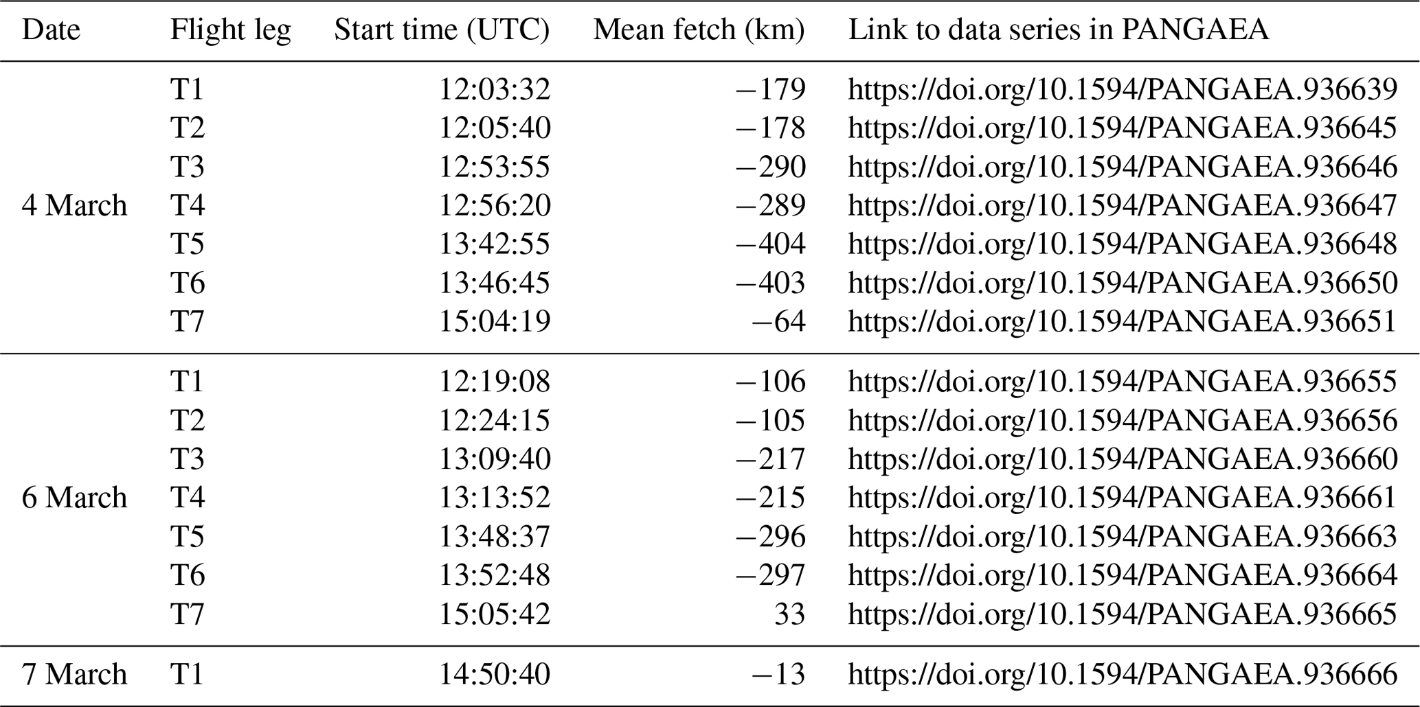
* The mean fetch along the flight tracks denotes the mean distance to the sea ice edge during the flight legs with negative (positive) values denoting flights over sea ice (open water). These distances were determined along the 5∘ E (4 March), 2.5∘ E (6 March), and 2∘ E (7 March) meridians respectively. All individual data series listed in the last column are also listed in Lüpkes et al. (2021a).
Table 2Overview of all dropsondes released on 4, 6, 7, and 26 March 2013.a

a The mean fetch denotes the mean distance to the sea ice edge along the flight track for each dropsonde. For 4, 6, and 7 March, these distances were determined along the 5∘ E (4 March), 2.5∘ E (6 March), and 2∘ E (7 March) meridians respectively. For 26 March, the values refer to the sea ice edge at 80.9∘ N and 17∘ E, which approximately marks the northeasternmost extension of the Whaler's Bay polynya on that day (see Fig. 1d). b This dropsonde was released at the same latitude as dropsonde D4 from the same day but more to the west and with a shorter fetch. c This dropsonde was released almost at the same position as dropsonde D2 from the same day but approximately 2 h 20 min earlier (see also Fig. 1). All individual data series listed in the last column are also listed in Lüpkes et al. (2021a).
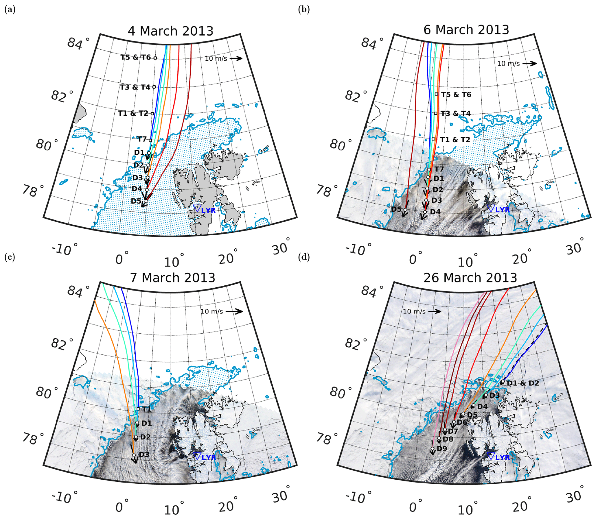
Figure 1Ice edge based on a 70 % threshold value of the ice concentration (derived with the Arctic Radiation and Turbulence Interaction Study, ARTIST, Sea Ice algorithm for the Advanced Microwave Scanning Radiometer 2; see Spreen et al., 2008) during MCAOs on (a) 4 March, (b) 6 March, (c) 7 March, and (d) 26 March 2013. The arrows denote the vertically ABL-averaged wind at the positions of the dropsondes listed in Table 2. In panels (a)–(c), locations of the aircraft profiles listed in Table 1 are shown. Coloured lines are backward trajectories obtained with the Hybrid Single-Particle Lagrangian Integrated Trajectory transport and dispersion model (Draxler and Rolph, 2010) at 10 m height from the positions of the dropsondes and of the southernmost aircraft vertical profiles for 4, 6, and 7 March. The backgrounds of panels (b)–(d) are the corresponding MODIS visible images at 13:10, 12:15, and 12:45 UTC respectively (data from https://lance.modaps.eosdis.nasa.gov/modis/, last access: 16 August 2021). Blue triangles mark the location of Longyearbyen airport (LYR). Modified based on Tetzlaff et al. (2014) and Tetzlaff (2016).
We present a data set that was collected during the STABLE campaign in the Fram Strait region north and west of Svalbard on 4, 6, 7, and 26 March 2013. The large-scale weather patterns on those days promoted the formation of strong MCAOs. The observations on 4, 6, and 7 March all concentrated on the same MCAO episode. During the course of 3 March, northerly winds and, thus, a strong off-ice flow developed in the lower troposphere over Fram Strait between a low-pressure system east of Svalbard and a strong high-pressure system over Greenland. These large-scale weather conditions more or less persisted for another 4 d, although the lower tropospheric flow turned slightly to the northwest in the southern part on 7 March (Fig. 1a, b, c). On 8 March, the MCAO weakened due to a high-pressure ridge that moved to the region west of Svalbard. The satellite images in Fig. 1 show that the MCAO affected the Whaler's Bay polynya – especially on 26 March. On that day, the flow almost had a northeast–southwest orientation (Fig. 1d) and was, thus, directed along the corresponding axis of the polynya. The corresponding large-scale weather pattern was characterised by a low-pressure system located at the southern tip of Svalbard, which had developed during the previous night.
The measurements during STABLE were performed with the Polar 5 research aircraft, a Basler BT-671. The following description of flight patterns and of the aircraft's instrumentation in Sect. 3.1 is partly based on Tetzlaff et al. (2014) and Tetzlaff (2016). Apart from observing MCAOs, an additional topic of STABLE was the measurement of ABL convection over leads in sea ice (mean and turbulent quantities). These measurements are described in detail by Tetzlaff et al. (2015), Tetzlaff (2016), and Michaelis et al. (2021), and the corresponding data can be found in Lüpkes et al. (2021b).
2.1 Flight patterns
All research flights (of typically 5–6 h duration) started and ended at the Longyearbyen airport (see also Fig. A1 in Appendix A). The measurements described in this paper took place between approximately 12:00 and 16:00 UTC on each day. Horizontally, they covered an area between approximately 78 and 84∘ N and between −5 and 25∘ E (Fig. 1). Basically, the flights were organised as follows. Especially over the open-ocean region with strong convective rolls and related clouds, flights were carried out at constant altitude of about 3000 m. There, the dropsondes were released. Prior to this, flight sections were flown north of the sea ice edge: these flights were mainly at low levels in the ABL, although some sections were also at 3000 m. These sections were interrupted at some points by ascents and descents to measure the vertical structure of the ABL. Cloud cover decreased during all flights towards the north, while the sea ice concentration increased to more than 90 %–95 % in this direction. The data set that we describe here was gained from the ascents and descents as well as from the dropsondes (see Fig. 1 and Tables 1–2).
For both 4 and 6 March, the data set consists of measurements from seven ascents and descents over the MIZ northwest of Svalbard (T1–T7) and of five dropsondes (D1–D5). On both days, the aircraft profiles T1–T6 were performed between about 40 m height and an altitude of 500–1000 m, which was above the shallow ABL. For these flight legs, the lower limits of the profiles were mostly determined by the low-level cloud conditions over sea ice. The remaining flight legs, abbreviated by T7 for both days, represent ascents performed up to almost 3000 m. For 7 March, measurements are only available from one ascent over the sea ice edge (T1) and from three dropsondes (D1–D3). For 26 March, only dropsonde measurements are included (D1–D9).
The dropsondes were mainly released over the open-ocean region between the sea ice edge and a few hundred kilometres downwind. Only three sondes were used north of the sea ice edge and, thus, over the sea-ice-covered region (D1 from 4 March as well as D1 and D2 from 26 March). On 4, 6, and 7 March, the ascents, descents, and dropsonde measurements were performed along a certain meridian. The meridional orientation of the flight patterns roughly corresponded to the main ABL flow direction in the MCAO as shown by the ABL-averaged winds at the dropsondes' positions (Fig. 1a, b, c). The corresponding MODIS visible images (for 6 and 7 March) denote that the main orientation of the cloud streets agreed well with the ABL-averaged winds on 7 March. However, a small shift is shown for 6 March, which might be due to the 3 h time difference between the satellite image and the dropsonde measurements (Fig. 1b). The MCAO observed on 26 March originated over the Whaler's Bay polynya so that the dropsonde measurements were performed along the main MCAO orientation from northeast to southwest (Fig. 1d).
3.1 Instrumentation
The data from the aircraft vertical profiles consist of high-frequency meteorological measurements and of measurements based on GPS and INS (Internal Navigation System) for position and altitude. Altitude is also provided based on the measured atmospheric static pressure. The corresponding offset in the original data, caused by the difference between the reference pressure at departure and the local near-surface pressure, was corrected using radar altimeter measurements during low-level flight legs between the vertical profiles. Differences between pressure and GPS height are explained in more detail in Sect. 3.2. Meteorological quantities were measured by instruments installed in and at the aircraft's nose-boom. Air pressure was measured with a five-hole probe, and the individual pressure components were then used to derive horizontal and vertical wind components. Note that we only provide mean meteorological quantities here, as the systematic determination of turbulent fluxes would have required different flight patterns. Vertical wind is only available as a deviation from the average value during horizontal flight sections (see also Ehrlich et al., 2019); thus, this quantity is also not provided in the final airborne data set. Temperature was measured with a Pt100 resistance thermometer, and relative humidity was measured with a dew point mirror. Pressure and temperature sensors responded fast enough to obtain a recording frequency of 100 Hz, whereas this value is lower for humidity (1 Hz). In the final, quality-controlled data set, all measurements are provided with a 100 Hz frequency, resulting in a vertical resolution of approximately 5 cm. Measurement accuracies are determined as ±0.1 hPa for pressure, ±0.01 K for temperature, ±0.4 % for the relative humidity readings, and ±0.2 m s−1 for the horizontal wind components (Hartmann et al., 2018). Note that the accuracy of humidity measurements, in particular, depends on environmental conditions. The given accuracy for the wind components is valid for horizontal flight legs and might, therefore, be worse during vertical profiles due to a different pressure field surrounding the aircraft (Hartmann et al., 2018). More details on the aircraft's instrumentation, the individual sensors, the calibration procedures, and the accuracies of the resulting data are provided in Hartmann et al. (2018) and Ehrlich et al. (2019, their Sect. 3.1).
3.2 Quality processing
Post-flight quality controlling for the airborne measurements included the interpolation of GPS and INS data to the time of the sensors installed at the turbulence nose boom. In addition, although there was not a standard procedure to remove spikes or outliers after the basic processing (as described in Hartmann et al., 2018) had been applied, all data series shown here were inspected visually. Sections of aircraft data where invalid values were identified (e.g. due to the influence by icing) have not been included in the data stored in the repository.
Air pressure data were corrected for the influence of the flow field around the aircraft. The corrected (static) air pressure ps was obtained as follows:
where ps,i is the uncorrected static pressure, qi is the uncorrected dynamic pressure, c is a calibration factor to obtain the corrected dynamic pressure (with c=1.165), and Δps is the measurement error of the five-hole probe depending on the flow angle (see Hartmann et al., 2018, their Eq. 6). The constant c was obtained by Hartmann et al. (2018) from several pairs of reverse-heading flight sections during which the mean wind only changed a little.
The wind components were calculated by the difference between the aircraft's velocity and the vector of the true airflow following the method described in detail by Hartmann et al. (2018). While the former component was obtained with a high accuracy from GPS and INS, the latter was obtained from the quality-controlled pressure measurements. Thus, for the wind components, there was no additional quality processing necessary apart from the manual check of all time series from which invalid sections had been removed. This also held for the humidity measurements.
Air temperature data were corrected for the adiabatic effect of the dynamic pressure originating from the motion of the aircraft. The following formula was applied:
where T is the corrected air temperature, TeN is the temperature measured by the sensor (in ∘C), qc is the quality-controlled dynamic pressure, R is the specific gas constant of dry air, and cp is the specific heat capacity of dry air at constant pressure. According to Eq. (2), temperatures are lower after the correction. For our aircraft data set, the average difference between uncorrected and corrected temperatures is 2–3 K. The maximum difference among all flight legs is almost 5 K.
In Fig. 2, we show the differences reported between the aircraft's altitude measured by GPS and that derived from the recorded and quality-controlled static pressure for each vertical profile. Mostly, the two data series differ by less than 10 m. Larger deviations are shown for some profiles of 4 March, peaking at a difference of more than 30 m on average for the T6 profile. For most profiles, the values measured by GPS were higher than the pressure-based values. This also holds for the height measurements of the dropsondes (see Sect. 4.2.1 and 4.2.3).
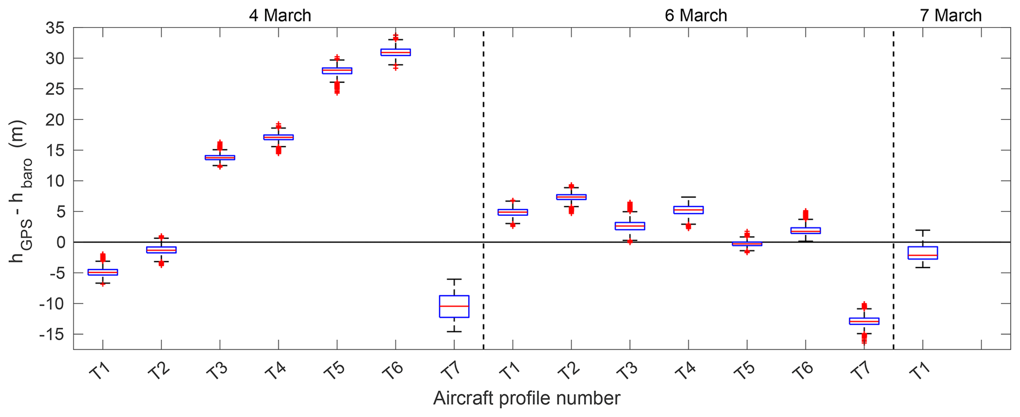
Figure 2Distribution of the differences between the aircraft's height measured by GPS (hGPS) and the corrected pressure altitude (hbaro) for each aircraft profile (see Table 1). Red lines show the median, the boxes are bounded by the upper and lower quartiles, the whiskers include the interval of approximately 99.7 % of the values, and red crosses denote outliers.
4.1 Instrumentation
The RD93 dropsondes (manufactured by Vaisala) were launched from the aircraft using the Airborne Vertical Atmosphere Profiling System (AVAPS, software version 1.7.1; see Ikonen et al., 2010) in its lite version, which can process only one dropsonde at a time (Vaisala, 2009). Here, we briefly summarise the main properties of both the sondes and the AVAPS based on the more detailed information given by Hock and Franklin (1999), Vaisala (2009), and Ikonen et al. (2010). Each sonde has a diameter of 7 cm; is 41 cm long; weighs about 390 g; and is equipped with temperature, humidity, and pressure sensors. Position, height, and wind speed and direction are derived from a GPS module that can track up to 12 satellites simultaneously. Pressure, temperature, and humidity measurements are collected by the AVAPS every 0.5 s, and GPS-derived wind is collected every 0.25 s. The AVAPS also reports the number of satellites used for the individual GPS-based measurements and the wind error. Following Hock and Franklin (1999), the latter is determined based on the measurement errors in the sondes' horizontal and vertical velocities and accelerations. The latter error consists of a random component (i.e. noise in the velocity estimates) and of a sampling component due to the sampling interval of the wind measurements (see Hock and Franklin, 1999).
Considering the sondes' fall rates of about −10 m s−1 during STABLE, a vertical resolution of approximately 2.5 m was obtained for wind, whereas the other meteorological quantities had a vertical resolution of approximately 5 m. Measurement accuracies are indicated by the manufacturer as 0.2 K for temperature, 0.4 hPa for pressure, 2 % for relative humidity (±2 % relative humidity for all readings), and 0.5 m s−1 for the horizontal wind speed (Vaisala, 2009). Following the remarks given by Hock and Franklin (1999), these values might be larger under non-laboratory conditions. For an older version of the Vaisala GPS dropsondes, the above-mentioned authors estimated measurement errors of 0.2 K for temperature, 1.0 hPa for pressure, < 5% for relative humidity, and 0.5–2 m s−1 for the horizontal wind speed (Hock and Franklin, 1999, their Table 3). As mentioned above, the magnitude of the latter error depends on the uncertainties in the position measurements via GPS. The measurements transmitted by each dropsonde were stored by the AVAPS as ascii-formatted text files, and we then applied quality-processing mechanisms to these files using ASPEN.
4.2 Quality processing
The need to apply quality processing to the raw dropsonde data from the STABLE campaign was shown by Tetzlaff (2016). They compared measurements of a dropsonde released over the MIZ with nearby airborne measurements obtained during an ascent and a descent. As stated by Tetzlaff (2016), the airborne measurements act as a useful reference for the dropsonde data due to the dropsonde's lower resolution and simpler instrumentation. The validation by Tetzlaff (2016) was performed over a region with 90 %–95 % sea ice cover on 20 March 2013. On this day, a stable boundary layer had developed due to on-ice flow conditions. The spatial difference between the aircraft profiles and the dropsonde was about 10 km near the release altitude and about 50 km near the surface. To focus only on sensor-related differences and to minimise the effects of surface-related spatial inhomogeneities, Tetzlaff (2016) selected measurements between 800 and 2000 m height for the comparison.
Tetzlaff (2016) found a very good agreement between the airborne and dropsonde measurements for wind despite the spatial differences. The average temperature measured with the dropsonde was 0.38 ∘C higher than during the aircraft profiles, which corresponded to twice the sensor's stated accuracy. The measured temperature variability was lower due to the lower sampling rate of the dropsonde's temperature sensor (Tetzlaff, 2016). Significant discrepancies occurred for relative humidity. The dropsonde data showed an absolute dry bias of 7 % compared with the relative humidity reading measured by aircraft (Tetzlaff, 2016). This was in agreement with the value from Vance et al. (2004), derived based on a comparison of the dropsonde type used with radiosonde and airborne data. In addition, the dropsonde's GPS sensor overestimated the altitude of the sonde by about 25 m (Tetzlaff, 2016). Thus, for the subsequent analysis of the dropsonde measurements in the MCAOs during STABLE, Tetzlaff (2016) and Tetzlaff et al. (2014) both used the pressure- and temperature-based geopotential height instead of the less reliable GPS height. They also removed data between the dropsonde release and the points where the sensors adapted to the ambient conditions in the atmosphere. Correction of the dry bias for humidity was not considered by the above-mentioned authors.
4.2.1 Correction mechanisms with the ASPEN software
To provide a reliable, quality-controlled dropsonde data set, we applied most of the standard quality-processing mechanisms implemented in ASPEN (see Martin and Suhr, 2021) for correcting the AVAPS raw data. Most of the following procedures have also been applied in other studies, for example, by Vömel et al. (2021) for their dropsonde data set. The individual steps are as follows:
-
The temperature-dependent dry bias for relative humidity is corrected using an algorithm provided by Vaisala (see also Vömel et al., 2016).
-
An ambient equilibration for pressure, temperature, and relative humidity is carried out. All data between the release of the sondes and the time after the individual sensors had adapted to the environmental atmospheric conditions (equilibration) were skipped by this correction. The range of the corresponding data being discarded was calculated by specifying the equilibration time as 7 times the individual sensors' time constants. Pressure and temperature equilibration times were set as equal. The largest equilibration time was applied for humidity, as the humidity sensor's time constant is largest. Using this correction, most of the data within the first 200–300 m of the launch point were discarded.
-
An ambient equilibration for wind, where 10 s was set as equilibration time, was carried out.
-
A post-splash check was undertaken. The three dropsondes released over the MIZ (see Table 2 and Sect. 2.1) still transmitted data after they had already reached the surface, which was automatically detected by ASPEN. The respective last relevant data points were then specified manually. All of the other dropsondes released over open water did not contain post-splash data.
-
A satellite check was run. A minimum of six satellites was set as a lower limit to ensure reliable GPS-based data (position, GPS height, fall velocity, and wind).
-
A wind error check was carried out. Wind measurements for which the corresponding error was higher than a certain threshold value were discarded. The threshold values specified in ASPEN are 1.5 m s−1 for measurements between 100 m and 10 km altitude and 1 m s−1 for measurements below 100 m and above 10 km.
-
Data points outside of predefined limits were removed. Lower and upper limits are specified in ASPEN as 0 and 1200 hPa for pressure, −100 and 50 ∘C for temperature, 0 % and 120 % for relative humidity, 0 and 150 m s−1 for wind speed, 0 and 360 ∘ for the wind direction, and −300 m and 40 000 m for the GPS altitude (adapted from https://ncar.github.io/aspendocs/algo_limitcheck.html, last access: 25 January 2022, Martin and Suhr, 2021).
-
Outliers were removed. Outliers are treated as a specified multiple of the standard deviation (σ) from a least-squares linear fit calculated for each data series. The multiples were specified as 4.5σ for pressure, 5σ for temperature, 10σ for relative humidity, and 5σ for the wind. These values correspond to the specifications suggested by the software developers for the dropsonde type used (see also https://ncar.github.io/aspendocs/algo_outlier.html, last access: 25 January 2022, Martin and Suhr, 2021).
-
Wild points were removed. These points refer to single data points that differ by more than a certain threshold value (specified in terms of change per unit in time) with respect to the neighbouring points. Similar to the outliers, these threshold values are also specified by the user. Here, we again chose the values suggested by the software developers. These are 1.5 hPa s−1 for pressure, 0.5 ∘C s−1 for temperature, 3 % s−1 for relative humidity, 0.005∘ s−1 for GPS latitude and longitude, 50 m s−1 for GPS altitude, and 10 m s−2 for wind speed.
-
A dynamic correction for wind and temperature was performed. This procedure helped to diminish errors caused by the temperature sensor's time lag (see also Sect. 4.2.2) and by the sonde's inertia that affected the wind determination.
-
Calculation of surface pressure and temperature by extrapolation was undertaken using the lowermost data point and the sonde's fall rate.
-
Calculation of the geopotential height was carried out based on pressure, temperature, and relative humidity. ASPEN uses upward integration starting from the surface or downward integration starting from the release altitude if the dropsonde does not transmit data until reaching the surface. For our dropsonde data, all dropsondes transmitted data to the surface; thus, we applied upward integration only (see Sect. 4.2.3 for more details).
-
A vertical (fall) velocity check was performed. The reliability of the dropsonde's horizontal wind measurements can be well linked to its fall velocity measured by GPS. ASPEN compares the GPS-based fall velocity to the hydrostatically derived fall velocity and the theoretical fall velocity. They are calculated based on the time-differentiated hydrostatic equation or based on the sonde's and parachute's aerodynamic properties using a model respectively. If the GPS-based fall velocity differed from the other two velocities by more than 2.5 m s−1, the corresponding wind measurements were discarded.
-
Calculation of the vertical wind component was undertaken. This quantity was calculated based on the parachute's area and the parachute drag coefficient. We specified those as 0.09 m2 and 0.61 respectively, following Wang et al. (2009).
More detailed explanations of these quality-processing mechanisms are given by Martin and Suhr (2021).
The removal of data points that did not pass the quality-processing procedures by ASPEN predominantly concerned the uppermost dropsonde measurements and, thus, regions where the sensors had not yet adapted to the ambient conditions after the sondes' releases. In addition, a small number of data, namely just 2–5 s measurement time of all sondes, was removed by the vertical fall velocity check. A removal of wind measurements with wind error values exceeding the limits also mostly concerned the measurements just below the aircraft.
Some of the uppermost GPS-derived data from the D5 sonde on 4 March, the D1 sonde on 6 March, and the D8 sonde on 26 March were removed because the minimum number of satellites required for the calculations was not reached. Hence, for the latter two sondes, GPS-derived data are not available for the uppermost 40–50 m after the pressure and temperature sensors had already adapted to the ambient conditions. For the D5 sonde from 4 March, GPS-derived data from the uppermost 200 m are missing in the quality-controlled data set, as the reported number of GPS satellites was zero at that time. In almost all dropsonde data series, a very small number of non-consecutive data points (mostly less than 10 per sonde) was removed by ASPEN because they were marked as having a cyclic redundancy check error for either the pressure–temperature unit or the GPS module.
4.2.2 Dry bias correction for humidity and dynamical adjustment
As expected, relative humidity values in the quality-controlled data are always higher than in the uncorrected data. Averaged over each data series, the correction ranges from +7.1 % to +9.9 % compared with the uncorrected relative humidity readings. These values correspond with the above-mentioned dry bias values found in previous studies (Vance et al., 2004; Tetzlaff, 2016).
The dynamical adjustment applied to the temperature and wind measurements is the only procedure that actually modifies the measured data (Martin and Suhr, 2021). Regarding the temperature data, the adjustment leads to a seemingly faster response of the dropsondes' temperature sensors to strong small-scale changes with height. This helps to overcome the lower temperature variability captured by the sondes compared with the aircraft measurements (see also Tetzlaff, 2016). We illustrate this effect in Fig. 3 for the three dropsondes that were released over sea ice. It is shown that the dynamical adjustment leads to more pronounced upper and lower boundaries of the temperature inversions, especially for those at a height of about 200–400 m, whereas the remaining measured temperature data are barely affected. For all dropsonde measurements, the average temperature of each profile only changed by about 0.05–0.25 K due to the dynamical adjustment. The dynamical adjustment for wind barely caused any change in the original wind values (not shown).
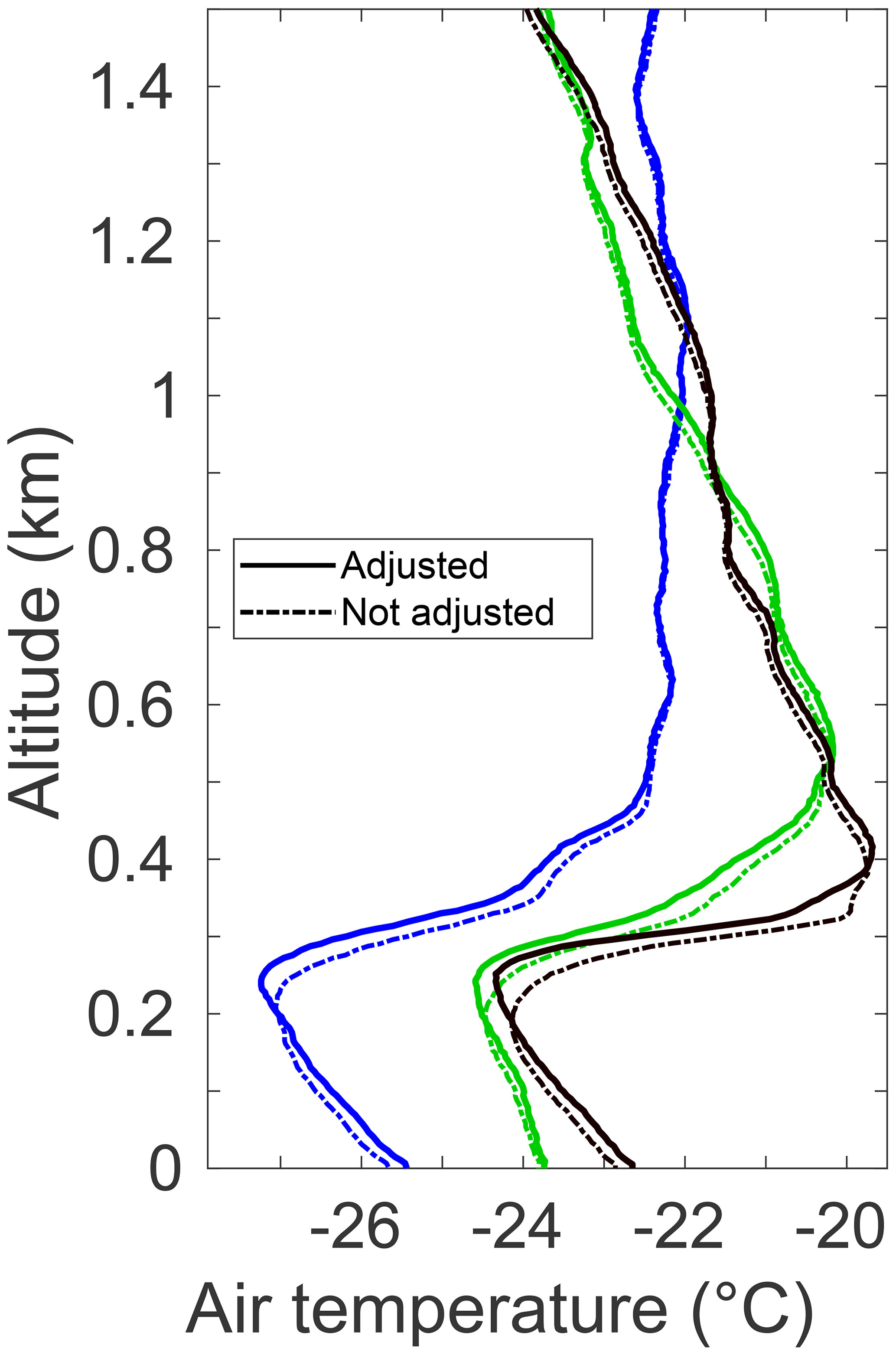
Figure 3Air temperature data of the D1 dropsonde from 4 March (blue) and the D1 (green) and D2 (dark red) dropsondes from 26 March (see Table 2) with and without the dynamical adjustment of ASPEN (see Martin and Suhr, 2021). Only the lowest 1.5 km of the profiles are shown.
4.2.3 Geopotential height calculation
As the three dropsondes that terminated over sea ice contained post-splash data, we can be sure that they transmitted data down to the surface. However, from the corresponding raw data series, we found that the GPS-based height delivered values of about 25–35 m at the point where the surface was reached. This discrepancy is similar to that described by Tetzlaff (2016). The other sondes transmitted data down to a GPS-derived height of about 25–50 m without containing post-splash data. This means that all of these sondes most probably reached the surface, although it is not indicated by the GPS-based height in the raw data. In addition, the sondes' measurements are transmitted at the end of the 0.5 s measurement cycle. This led to a loss of data for the lowermost few metres for the sondes not reporting post-splash data (Hock and Franklin, 1999). For these two reasons, we can, however, assume that the corresponding sondes successfully transmitted data until they reached the sea surface. The sondes' surface data, which were then required to perform the upward integration of the geopotential height, were computed in ASPEN via extrapolation from the lowermost measurements transmitted. The upward integration was then performed until the uppermost quality-controlled pressure value was reached. In most cases, the uppermost quality-controlled pressure value was at a lower altitude than the uppermost GPS-derived wind values due to the different equilibration times for the corresponding sensors (Sect. 4.2.1). Thus, no geopotential altitude could be obtained for a few of the uppermost quality-controlled wind data points.
4.2.4 Wind speed error
As explained in Sect. 4.2.1, wind measurements exceeding a certain error threshold are discarded by ASPEN. In Fig. 4, we show the distribution of the wind error for the remaining quality-controlled wind data. It is shown that the median as well as the lower and upper quartiles of the wind error are between 0.4 and 0.7 m s−1 in most cases. Moreover, for all sondes, the whiskers in Fig. 4 denote that approximately 99.7 % of the wind error values are between 0.4 and 0.9 m s−1. However, for some data points, the wind error amounts to almost 1.5 m s−1.

For model validation, the dropsondes' drift distances and the flight distances during the aircraft's descents/ascents might be important; thus, we provide this information in Fig. 5. As we decided to plot the distances against the pressure-based altitude and not against the value based on GPS, the dropsondes' drift distances (Fig. 5a, b, c, d) are not shown for the layer where the meteorological sensors had not yet adapted to the environmental atmospheric conditions after release (see also Sect. 4.2.1). We also added the release altitudes of all sondes in Fig. 5a–d, where this information is only available from GPS. Most of the sondes showed a monotonic drift that was generally along the main flow direction in the respective MCAO, except for D2 from 6 March. Especially on 26 March, some sondes drifted faster in the lowest kilometre of the atmosphere than at higher altitudes. This indicates a stronger wind speed in the convective ABL compared with the free atmosphere (see also Chechin et al., 2013). None of the sondes drifted more than 5 km, and the strongest drifts were observed on 4 March.
Due to the small inclination of the aircraft during the vertical profiles (trajectory angles between −3 and −5∘ for descents and between 5 and 8∘ for ascents, on average), the travel distance and, thus, the horizontal distance of the measurements during one descent/ascent was much higher than for the dropsondes. During STABLE, these horizontal distances summed to 30–40 km for an ascent from the surface to 3 km altitude (Fig. 5e, f, g). During the shorter profiles over the MIZ further north, the horizontal travel distance was mostly in the range from 2 to 13 km.
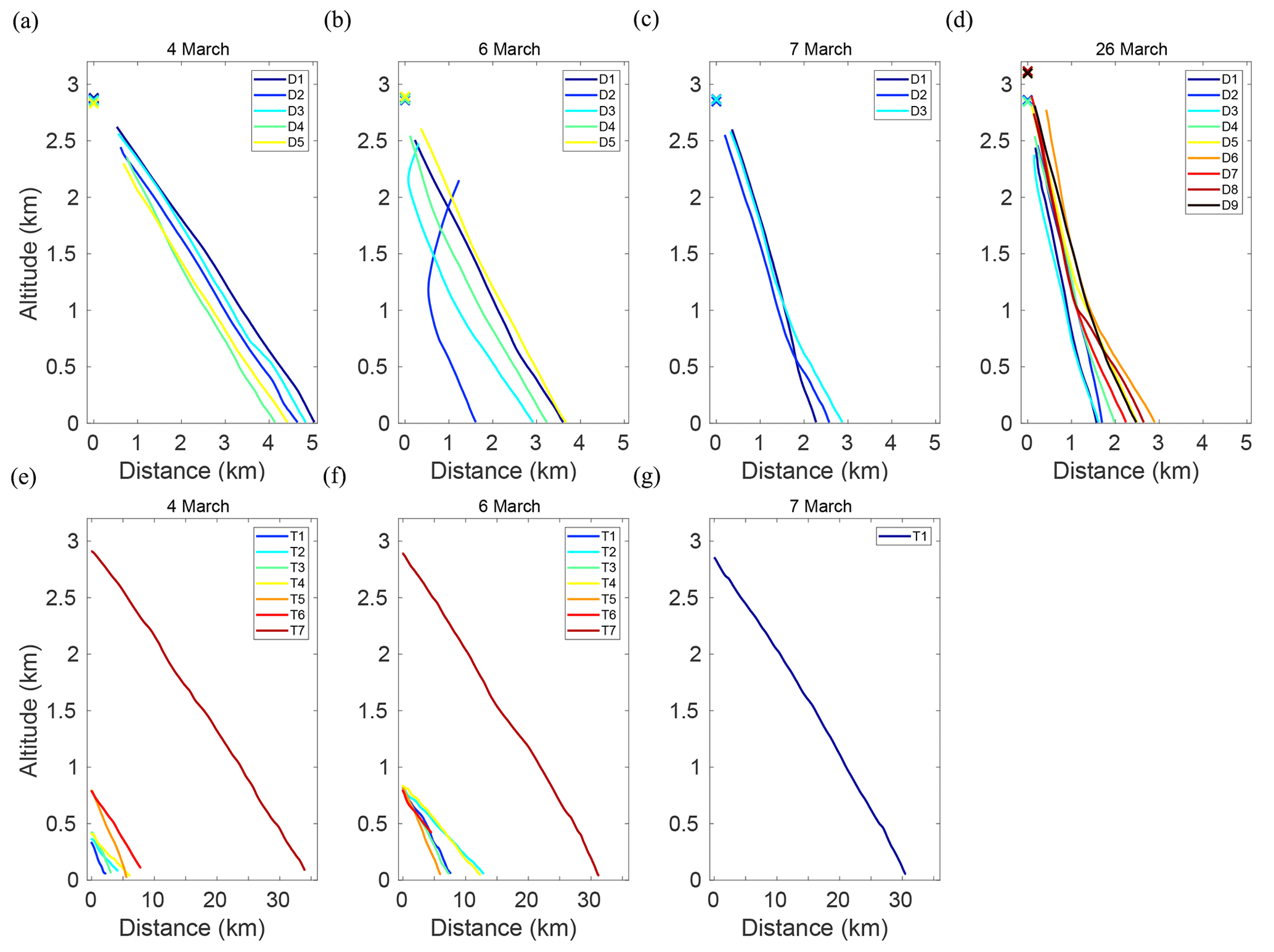
Figure 5Horizontal drift distances of the dropsondes (a–d) and distances flown by the aircraft during ascents and descents (e–g). Distances are calculated with respect to the uppermost measurement point. For the dropsondes, this information is missing for the uppermost layer (see text), and coloured crosses refer to the dropsondes' release altitudes derived via GPS.
In this section, we focus on the meteorological characteristics of the MCAOs based on the quality-controlled airborne and dropsonde data. Figures 6 and 7 show vertical cross sections of temperature, wind speed, and specific and relative humidity. For the latter quantity, it should be noted that we only show those regions where saturation over ice was reached, indicating that clouds had presumably been present. Figures B1 and B2 in Appendix B show the total values of relative humidity. All cross sections are designed in a similar way to those shown in Tetzlaff et al. (2014) for potential temperature and in Tetzlaff (2016) for all four variables. The data from the aircraft's profiles in the above-mentioned work are the same as those in our illustrations, whereas different corrections were applied to the dropsonde data (see Sect. 4.2.1). Figures 6 and 7 also show the ABL height on each day, which was adapted from Tetzlaff (2016). We provide only a brief description of the cross sections and refer to Tetzlaff et al. (2014) and Tetzlaff (2016) for a more detailed interpretation.
6.1 MCAO episode from 4 to 7 March
On 4 March, the observed MCAO was characterised by a shallow, slightly stably stratified ABL of about 250 m depth over sea ice and by a strong increase in both the ABL height and temperature with increasing distance over open water (Fig. 6a). As noted by Tetzlaff et al. (2014), the resulting ABL height of about 2500 m at a distance of 214 km was extraordinarily high compared with MCAOs observed in the early 1990s (e.g. Brümmer, 1997). A strong increase with increasing distance was also observed for both specific humidity and horizontal wind speed inside the ABL (Fig. 6c, e). The relative humidity distribution depicts clouds in the entire ABL over open water with an increasing cloud base and top further to the south (Fig. 6g). Another shallow cloud layer is denoted above the ABL at about 50 km distance. Moreover, it is shown that clouds were presumably also present over sea ice on that day, except for the northernmost flight legs. This agrees with visual observations made by the participants of the corresponding research flight.
On 6 March, the ABL over sea ice was slightly shallower than 2 d before. Moreover, the increase in both temperature and the ABL height with increasing distance was not as pronounced as on 4 March (Fig. 6b). The specific humidity distribution denotes a slightly more humid ABL over sea ice but a similarly humid ABL over open water compared with 4 March (Fig. 6d). Horizontal winds basically decreased from 4 to 6 March, especially over open water (Fig. 6f). The relative humidity distribution denotes the presence of clouds over both sea ice and the open ocean. Compared with 4 March, less clouds might have been present over sea ice on 6 March (Fig. 6h).
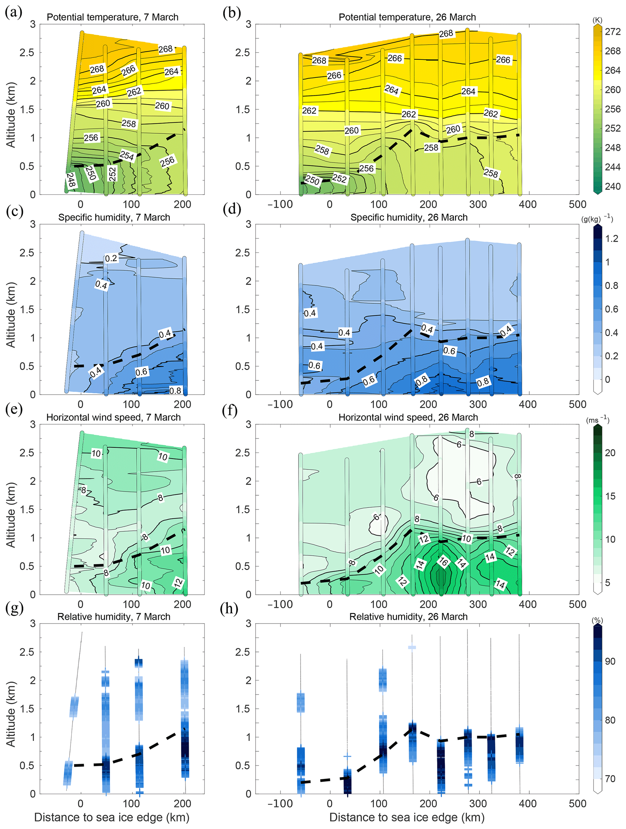
Unlike the previous 2 d, no airborne measurements are available for the MIZ region on 7 March. The corresponding cross sections indicate a weakening of the MCAO compared with 4 and 6 March. Namely, specific humidity and horizontal wind speed in the ABL over open water were lower than on 4 and 6 March (Fig. 7a, c, e). Furthermore, the increases in temperature and in the ABL with increasing distance were less strong. The corresponding relative humidity distribution (Fig. 7g) denotes several clouds not only in but also above the ABL along the entire cross section.
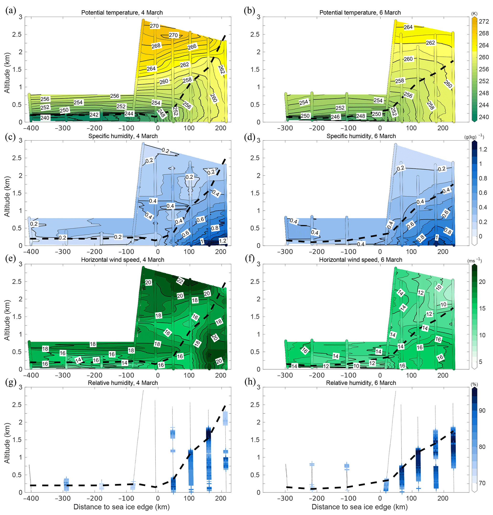
Figure 6Vertical cross sections of (a–b) potential temperature, (c–d) specific humidity, (e–f) horizontal wind speed, and (g–h) relative humidity in saturated areas with respect to an ice surface for (a, c, e, g) 4 March and (b, d, f, h) 6 March 2013 based on the quality-controlled airborne and dropsonde measurements. The flow is from left to right so that negative (positive) distances correspond to sea ice (open water). Dashed black lines denote the ABL height. Modified based on Tetzlaff et al. (2014) and Tetzlaff (2016).
6.2 MCAO event on 26 March
The measurements of the D2–D5 dropsondes, which were released almost exactly along the main ABL flow direction in the MCAO, denote a deepening of the ABL from a height of approximately 250 m near −50 km distance over the MIZ to a height of 1250 m at about 160 km distance over open water (Fig. 7b). This coincides with a potential temperature increase in the ABL from approximately 248 to 258 K and a slight increase in both specific humidity and horizontal wind speed (Fig. 7b, d, f). Figure 7h shows that clouds were presumably present in the entire ABL along the MCAO orientation and also above the ABL over the polynya region. In the region further downwind where the D6–D9 dropsondes were released, the ABL-averaged wind direction had turned slightly to north (see Fig. 1d), and the ABL had not deepened further with increasing fetch.
The data are available from the PANGAEA repository (Lüpkes et al., 2021a). All 37 data series can be found at https://doi.org/10.1594/PANGAEA.936635 along with a brief data description. The individual DOIs of each data series are also listed in Tables 1 and 2 in this paper. All data series are provided as tab-delimited text files (ascii). Missing or discarded measurements are indicated by empty fields in those files, although this only concerns the dropsonde data. All data are supplemented by metadata with information on the location and time of the measurements, the corresponding event, and the measured quantities.
The STABLE aircraft campaign was performed in March 2013. One of its main objectives was the investigation of atmospheric convection and boundary layer modifications associated with marine cold-air outbreaks (MCAOs). MCAOs occurring over the Fram Strait region were observed on 4 d using highly resolved atmospheric measurements from instruments mounted in and at the aircraft's nose boom and by dropsondes. The observations took place during a period with an unusually large Whaler's Bay polynya north of Svalbard, which also led to extraordinarily deep convective boundary layers during the MCAOs only 200–250 km south of the ice edge (see Tetzlaff et al., 2014, and Tetzlaff, 2016). We have given a detailed description of the corresponding data from a total of 15 aircraft vertical profiles and 22 dropsondes. Data from the aircraft's profiles predominantly referred to observations over the marginal sea ice zone up to about 400 km upwind of the ice edge, whereas most of the dropsonde measurements took place over the open ocean. Thus, the research flights were arranged to allow detailed lower-tropospheric observations ranging from the MCAO source regions far north of the ice margin to the open-ocean region with the evolving convective boundary layers. Moreover, the flights approximately followed the mean wind direction.
To obtain a high-quality data set, we applied several quality-processing steps for both aircraft and dropsonde measurements. Especially for the dropsonde data, multiple corrections had to be applied. Thus, we used quality-processing algorithms implemented in the Atmospheric Sounding Processing Environment (ASPEN; Martin and Suhr, 2021) software. This did not only help to remove suspicious data points but also, for example, to correct the dry bias found in the dropsonde measurements of relative humidity (see Vance et al., 2004). Moreover, a dynamical adjustment applied to the dropsondes' temperature measurements improved the representation of the observed temperature inversions and generally helped to overcome the reduction in the captured temperature variability compared with the aircraft measurements.
Our data set refers to observations of one MCAO episode lasting for 3 d and to an MCAO that directly affected the Whaler's Bay polynya. This tenders at least two possible uses for these data in further studies: (1) they could be utilised for the exploration of the temporal and spatial variability of the MCAO episode from 4 to 7 March 2013, and (2) the data could act as a reference for investigations of MCAOs under an extremely small springtime Arctic sea ice cover north of Svalbard. Thus, the data may be useful for micro- and mesoscale process-oriented modelling approaches (as in work such as Lüpkes and Schlünzen, 1996; Gryschka et al., 2008; Gryschka et al., 2014; and Chechin et al., 2013) as well as for larger-scale projections that assume an extremely low ice concentration north of Svalbard such as that observed during STABLE.
Altogether, the data set that we presented here consists of reliable and highly resolved atmospheric measurements of temperature, humidity, wind, and pressure. It provides a detailed representation of the vertical structure of the lower troposphere inside and above the evolving boundary layers during the MCAOs. Thus, it might serve as a valuable reference for comparisons with other observational data as well as for the validation of model simulation results for such polar air mass transformation events.
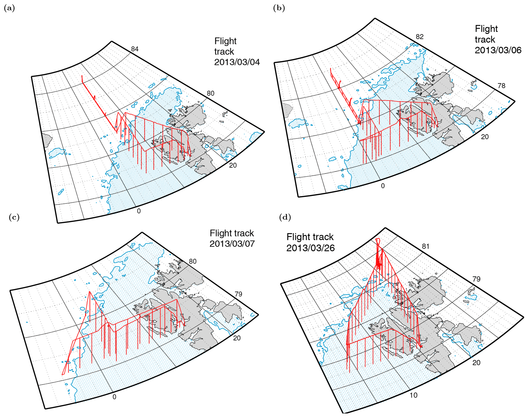
Figure A1A 3D illustration of the flight tracks on 4 March (a), 6 March (b), 7 March (c), and 26 March 2013 (d) plotted over the ice edge based on a 70 % threshold value of the ice concentration (see also Fig. 1 in Sect. 2). The length of the vertical lines between the flight tracks and the surface indicates the height of the aircraft during the research flights.
Figure A1 illustrates the flight tracks of the research flights from STABLE on 4, 6, 7, and 26 March 2013. On 4 and 6 March, the flight patterns mainly consisted of meridionally oriented flight legs in the region of the MCAOs (see also Sect. 2.1). On 7 March, additional measurements were performed during a low-level flight leg nearly parallel to the ice margin west of Svalbard. On 26 March, airborne measurements were performed over a lead located near 81.6∘ N and 21.4∘ E (see also Tetzlaff et al., 2015; Michaelis et al., 2021) prior to the measurements in the MCAO that occurred over the Whaler's Bay polynya.
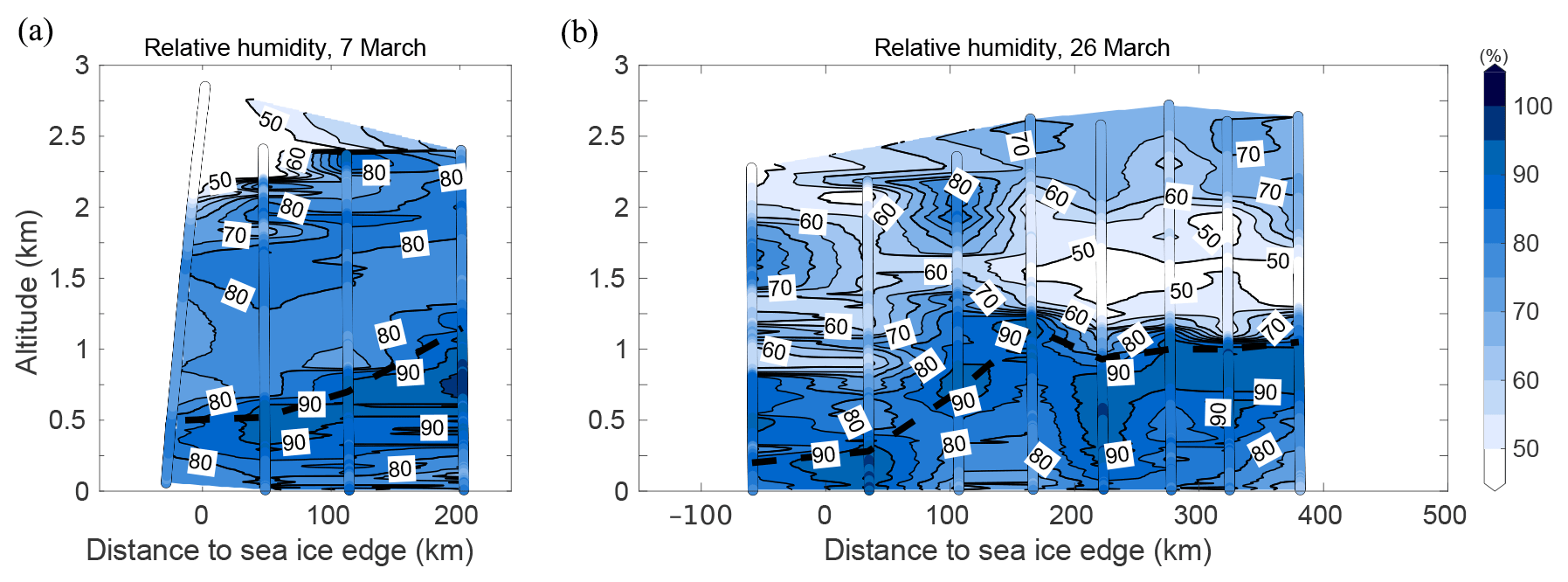
Similar to panels g and h in Figs. 6 and 7 (shown in Sect. 6), we provide vertical cross sections of the relative humidity based on the airborne and dropsonde measurements for 4, 6, 7, and 26 March 2013 in the respective MCAOs in Figs. B1 and B2. Unlike the corresponding panels in Sect. 6, we show the distribution of the total relative humidity in this section. While panels g and h in Figs. 6 and 7 helped to detect regions of saturated air and, thus, clouds, Figs. B1 and B2 help to better identify dry and humid regions in the atmosphere roughly along the main MCAO orientations. For example, it is clearly shown that the region of the free atmosphere above the convective ABL over open water was basically much drier on 4 March than on 6 March (Fig. B1a, b). Low relative humidity is also shown above the temperature inversion on 26 March, starting at a fetch of about 150 km (Fig. B2b).
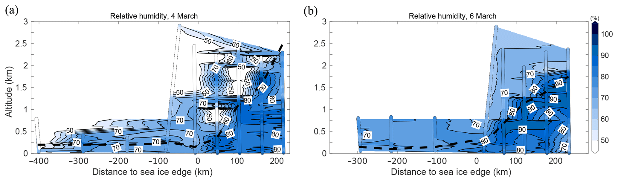
Figure B1Same as Fig. 6, but vertical cross sections are shown for the total values of relative humidity on (a) 4 March and (b) 6 March 2013. Modified based on Tetzlaff et al. (2014) and Tetzlaff (2016).
AS, CL, JH, GB, and TV all participated in planning the research flights during STABLE, and they operated the instruments onboard the aircraft, including the AVAPS dropsonde system. The quality processing was performed by JH for the aircraft data and by JM for the dropsonde data using the ASPEN dropsonde software. Data visualisation was done by JM with contributions from AS. JM performed the data analyses and prepared the manuscript. All co-authors contributed to the final writing of the paper.
The contact author has declared that neither they nor their co-authors have any competing interests.
Publisher’s note: Copernicus Publications remains neutral with regard to jurisdictional claims in published maps and institutional affiliations.
We gratefully acknowledge funding from the Deutsche Forschungsgemeinschaft (DFG, German Research Foundation; project no. 268020496 – TRR 172) within the framework of the Transregional Collaborative Research Centre: “ArctiC Amplification: Climate Relevant Atmospheric and SurfaCe Processes, and Feedback Mechanisms (AC)3”. We are grateful to all aircraft engineers and the flight crew for their support during the campaign. We also thank Andreas Walbröl and Jan Chylik for helpful comments. Finally, we thank Ian Brooks and an anonymous reviewer for their constructive criticism that helped to improve the paper.
This research has been supported by the Deutsche Forschungsgemeinschaft (grant no. 268020496 – TRR 172).
This paper was edited by Ge Peng and reviewed by Ian Brooks and one anonymous referee.
Brümmer, B.: Boundary-layer modification in wintertime cold-air outbreaks from the Arctic sea ice, Bound-Lay. Meteorol., 80, 109–125, https://doi.org/10.1007/BF00119014, 1996. a
Brümmer, B.: Boundary layer mass, water, and heat budgets in wintertime cold-air outbreaks from the Arctic sea ice, Mon. Weather Rev., 125, 1824–1837, https://doi.org/10.1175/1520-0493(1997)125<1824:BLMWAH>2.0.CO;2, 1997. a, b
Brümmer, B.: Roll and cell convection in wintertime Arctic cold-air outbreaks, J. Atmos. Sci., 56, 2613–2636, https://doi.org/10.1175/1520-0469(1999)056<2613:RACCIW>2.0.CO;2, 1999. a
Brümmer, B. and Pohlmann, S.: Wintertime roll and cell convection over Greenland and Barents Sea regions: A climatology, J. Geophys. Res.-Atmos., 105, 15559–15566, https://doi.org/10.1029/1999JD900841, 2000. a, b
Brümmer, B., Rump, B., and Kruspe, G.: A cold air outbreak near Spitsbergen in springtime—Boundary-layer modification and cloud development, Bound-Lay. Meteorol., 61, 13–46, https://doi.org/10.1007/BF02033993, 1992. a
Cavalieri, D. J. and Parkinson, C. L.: Arctic sea ice variability and trends, 1979–2010, The Cryosphere, 6, 881–889, https://doi.org/10.5194/tc-6-881-2012, 2012. a
Chechin, D. G. and Lüpkes, C.: Boundary-layer development and low-level baroclinicity during high-latitude cold-air outbreaks: A simple model, Bound-Lay. Meteorol., 162, 91–116, https://doi.org/10.1007/s10546-016-0193-2, 2017. a
Chechin, D. G., Lüpkes, C., Repina, I. A., and Gryanik, V. M.: Idealized dry quasi 2-D mesoscale simulations of cold-air outbreaks over the marginal sea ice zone with fine and coarse resolution, J. Geophys. Res.-Atmos., 118, 8787–8813, https://doi.org/10.1002/jgrd.50679, 2013. a, b, c
Draxler, R. R. and Rolph, G. D.: HYSPLIT (HYbrid Single-Particle Lagrangian Integrated Trajectory) model access via NOAA ARL READY website, NOAA Air Resources Laboratory, Silver Spring, MD, 25, http://ready.arl.noaa.gov/HYSPLIT.php (last access: 22 July 2021), 2010. a
Ehrlich, A., Wendisch, M., Lüpkes, C., Buschmann, M., Bozem, H., Chechin, D., Clemen, H.-C., Dupuy, R., Eppers, O., Hartmann, J., Herber, A., Jäkel, E., Järvinen, E., Jourdan, O., Kästner, U., Kliesch, L.-L., Köllner, F., Mech, M., Mertes, S., Neuber, R., Ruiz-Donoso, E., Schnaiter, M., Schneider, J., Stapf, J., and Zanatta, M.: A comprehensive in situ and remote sensing data set from the Arctic CLoud Observations Using airborne measurements during polar Day (ACLOUD) campaign, Earth Syst. Sci. Data, 11, 1853–1881, https://doi.org/10.5194/essd-11-1853-2019, 2019. a, b
Etling, D. and Brown, R. A.: Roll vortices in the planetary boundary layer: A review, Bound-Lay. Meteorol., 65, 215–248, https://doi.org/10.1007/BF00705527, 1993. a
Fletcher, J., Mason, S., and Jakob, C.: The climatology, meteorology, and boundary layer structure of marine cold air outbreaks in both hemispheres, J. Climate, 29, 1999–2014, https://doi.org/10.1175/JCLI-D-15-0268.1, 2016. a
Geerts, B., McFarquhar, G., Xue, L., Jensen, M., Kollias, P., Ovchinnikov, M., Shupe, M., DeMott, P., Wang, Y., Tjernström, M., Field, P., Abel, S., Spengler, T., Neggers, R., Crewell, S., Wendisch, M., and Lüpkes, C.: Cold-Air Outbreaks in the Marine Boundary Layer Experiment (COMBLE) Field Campaign Report, DOE/SC-ARM-21-001, https://www.arm.gov/publications/programdocs/doe-sc-arm-21-001.pdf (last access: 31 January 2022), 2021. a
Gryanik, V. M. and Hartmann, J.: A turbulence closure for the convective boundary layer based on a two-scale mass-flux approach, J. Atmos. Sci., 59, 2729–2744, https://doi.org/10.1175/1520-0469(2002)059<2729:ATCFTC>2.0.CO;2, 2002. a
Gryschka, M., Drüe, C., Etling, D., and Raasch, S.: On the influence of sea-ice inhomogeneities onto roll convection in cold-air outbreaks, Geophys. Res. Lett., 35, L23804, https://doi.org/10.1029/2008GL035845, 2008. a, b
Gryschka, M., Fricke, J., and Raasch, S.: On the impact of forced roll convection on vertical turbulent transport in cold air outbreaks, J. Geophys. Res.-Atmos., 119, 12–513, https://doi.org/10.1002/2014JD022160, 2014. a, b
Hartmann, J., Kottmeier, C., and Raasch, S.: Roll vortices and boundary-layer development during a cold air outbreak, Bound-Lay. Meteorol., 84, 45–65, https://doi.org/10.1023/A:1000392931768, 1997. a
Hartmann, J., Gehrmann, M., Kohnert, K., Metzger, S., and Sachs, T.: New calibration procedures for airborne turbulence measurements and accuracy of the methane fluxes during the AirMeth campaigns, Atmos. Meas. Tech., 11, 4567–4581, https://doi.org/10.5194/amt-11-4567-2018, 2018. a, b, c, d, e, f, g
Hock, T. F. and Franklin, J. L.: The NCAR GPS dropwindsonde, B. Am. Meteorol. Soc., 80, 407–420, https://doi.org/10.1175/1520-0477(1999)080<0407:TNGD>2.0.CO;2, 1999. a, b, c, d, e, f
Ikonen, I., Demetriades, N. W. S., and Holle, R. L.: Vaisala dropsondes: History, status, and applications, in: 29th Conference on Hurricanes and Tropical Meteorology, Tucson, Arizona, 10–14 May 2010, https://ams.confex.com/ams/29Hurricanes/webprogram/Paper168031.html (last access: 1 February 2022), 2010. a, b
Kolstad, E. W. and Bracegirdle, T. J.: Marine cold-air outbreaks in the future: An assessment of IPCC AR4 model results for the Northern Hemisphere, Clim. Dynam., 30, 871–885, https://doi.org/10.1007/s00382-007-0331-0, 2008. a
Landgren, O. A., Seierstad, I. A., and Iversen, T.: Projected future changes in Marine Cold-Air Outbreaks associated with Polar Lows in the Northern North-Atlantic Ocean, Clim. Dynam., 53, 2573–2585, https://doi.org/10.1007/s00382-019-04642-2, 2019. a
Liu, A. Q., Moore, G. W. K., Tsuboki, K., and Renfrew, I. A.: The effect of the sea-ice zone on the development of boundary-layer roll clouds during cold air outbreaks, Bound-Lay. Meteorol., 118, 557–581, https://doi.org/10.1007/s10546-005-6434-4, 2006. a
Lüpkes, C. and Schlünzen, K. H.: Modelling the Arctic convective boundary-layer with different turbulence parameterizations, Bound-Lay. Meteorol., 79, 107–130, https://doi.org/10.1007/BF00120077, 1996. a, b
Lüpkes, C., Vihma, T., Birnbaum, G., Dierer, S., Garbrecht, T., Gryanik, V. M., Gryschka, M., Hartmann, J., Heinemann, G., Kaleschke, L., Raasch, S., Savijärvi, H., Schlünzen, K. H., and Wacker, U.: Mesoscale modelling of the Arctic atmospheric boundary layer and its interaction with sea ice, in: Arctic Climate Change, Springer, 279–324, 2012. a
Lüpkes, C., Hartmann, J., Schmitt, A. U., Birnbaum, G., Vihma, T., and Michaelis, J.: Airborne and dropsonde measurements in MCAOs during STABLE in March 2013, PANGAEA [data set], https://doi.org/10.1594/PANGAEA.936635, 2021a. a, b, c, d, e
Lüpkes, C., Hartmann, J., Schmitt, A. U., and Michaelis, J.: Convection over sea ice leads: Airborne measurements of the campaign STABLE from March 2013, PANGAEA [data set], https://doi.org/10.1594/PANGAEA.927260, 2021b. a
Martin, C. and Suhr, I.: NCAR/EOL Atmospheric Sounding Processing ENvironment (ASPEN) software. Version 3.4.6, https://www.eol.ucar.edu/content/aspen, last access: 20 May 2021. a, b, c, d, e, f, g, h
Michaelis, J., Lüpkes, C., Schmitt, A. U., and Hartmann, J.: Modelling and parametrization of the convective flow over leads in sea ice and comparison with airborne observations, Q. J. Roy. Meteor. Soc., 147, 914–943, https://doi.org/10.1002/qj.3953, 2021. a, b
Pithan, F., Svensson, G., Caballero, R., Chechin, D., Cronin, T. W., Ekman, A. M., Neggers, R., Shupe, M. D., Solomon, A., Tjernström, M., and Wendisch, M.: Role of air-mass transformations in exchange between the Arctic and mid-latitudes, Nat. Geosci., 11, 805–812, https://doi.org/10.1038/s41561-018-0234-1, 2018. a
Rasmussen, E. A.: Polar lows, in: A Half Century of Progress in Meteorology: A Tribute to Richard Reed, Springer, 61–78, 2003. a
Spreen, G., Kaleschke, L., and Heygster, G.: Sea ice remote sensing using AMSR-E 89-GHz channels, J. Geophys. Res.-Oceans, 113, C02S03, https://doi.org/10.1029/2005JC003384, 2008. a
Tetzlaff, A.: Convective processes in the polar atmospheric boundary layer: a study based on measurements and modeling, Doctoral dissertation, University of Bremen, Germany, 136 pp., http://nbn-resolving.de/urn:nbn:de:gbv:46-00105016-14 (last access: 31 January 2022), 2016. a, b, c, d, e, f, g, h, i, j, k, l, m, n, o, p, q, r, s, t, u, v, w, x, y
Tetzlaff, A., Lüpkes, C., Birnbaum, G., Hartmann, J., Nygård, T., and Vihma, T.: Brief Communication: Trends in sea ice extent north of Svalbard and its impact on cold air outbreaks as observed in spring 2013, The Cryosphere, 8, 1757–1762, https://doi.org/10.5194/tc-8-1757-2014, 2014. a, b, c, d, e, f, g, h, i, j, k, l, m, n
Tetzlaff, A., Lüpkes, C., and Hartmann, J.: Aircraft-based observations of atmospheric boundary-layer modification over Arctic leads, Q. J. Roy. Meteor. Soc., 141, 2839–2856, https://doi.org/10.1002/qj.2568, 2015. a, b
Vaisala: Vaisala Dropsonde RD93, http://www.vaisala.com (last access: 02 February 2022), 2009. a, b, c
Vance, A. K., Taylor, J. P., Hewison, T. J., and Elms, J.: Comparison of in situ humidity data from aircraft, dropsonde, and radiosonde, J. Atmos. Ocean. Tech., 21, 921–932, https://doi.org/10.1175/1520-0426(2004)021<0921:COISHD>2.0.CO;2, 2004. a, b, c
Vihma, T., Pirazzini, R., Fer, I., Renfrew, I. A., Sedlar, J., Tjernström, M., Lüpkes, C., Nygård, T., Notz, D., Weiss, J., Marsan, D., Cheng, B., Birnbaum, G., Gerland, S., Chechin, D., and Gascard, J. C.: Advances in understanding and parameterization of small-scale physical processes in the marine Arctic climate system: a review, Atmos. Chem. Phys., 14, 9403–9450, https://doi.org/10.5194/acp-14-9403-2014, 2014. a
Vömel, H., Young, K., and Hock, T.: NCAR GPS Dropsonde Humidity Dry Bias, Tech. rep., National Center for Atmospheric Research Boulder, Colorado, 10 pp., https://www.aoml.noaa.gov/hrd/Storm_pages/Dropsonde_Dry_Bias_TN_531.pdf (last access: 25 January 2022), 2016. a
Vömel, H., Goodstein, M., Tudor, L., Witte, J., Fuchs-Stone, Ž., Sentić, S., Raymond, D., Martinez-Claros, J., Juračić, A., Maithel, V., and Whitaker, J. W.: High-resolution in situ observations of atmospheric thermodynamics using dropsondes during the Organization of Tropical East Pacific Convection (OTREC) field campaign , Earth Syst. Sci. Data, 13, 1107–1117, https://doi.org/10.5194/essd-13-1107-2021, 2021. a
Wang, J., Bian, J., Brown, W. O., Cole, H., Grubišić, V., and Young, K.: Vertical air motion from T-REX radiosonde and dropsonde data, J. Atmos. Ocean. Tech., 26, 928–942, https://doi.org/10.1175/2008JTECHA1240.1, 2009. a
Zahn, M. and von Storch, H.: Decreased frequency of North Atlantic polar lows associated with future climate warming, Nature, 467, 309–312, https://doi.org/10.1038/nature09388, 2010. a
For more information, the reader is referred to https://www.awi.de/en/expedition/aircraft/polar-5-6.html (last access: 25 January 2022)
- Abstract
- Introduction
- The STABLE campaign
- Aircraft measurements
- Dropsonde measurements
- Horizontal distance
- Cold-air outbreaks
- Data availability
- Conclusions
- Appendix A: Flight tracks
- Appendix B: Vertical cross sections of relative humidity
- Author contributions
- Competing interests
- Disclaimer
- Acknowledgements
- Financial support
- Review statement
- References