the Creative Commons Attribution 4.0 License.
the Creative Commons Attribution 4.0 License.
 | 07 Apr 2022
A new dataset of river flood hazard maps for Europe and the Mediterranean Basin
Francesco Dottori
Lorenzo Alfieri
Alessandra Bianchi
Jon Skoien
Peter Salamon
In recent years, the importance of continental-scale hazard maps for riverine floods has grown. Nowadays, such maps are used for a variety of research and commercial activities, such as evaluating present and future risk scenarios and adaptation strategies, as well as supporting management plans for national and local flood risk. In this paper we present a new set of high-resolution (100 m) hazard maps for river flooding that covers most European countries, as well as all of the river basins entering the Mediterranean and Black Sea in the Caucasus, the Middle East and northern Africa. The new river flood hazard maps represent inundation along 329 000 km of the river network, for six different flood return periods, expanding on the datasets previously available for the region. The input river flow data for the new maps are produced by means of the hydrological model LISFLOOD using new calibration and meteorological data, while inundation simulations are performed with the hydrodynamic model LISFLOOD-FP. In addition, we present here a detailed validation exercise using official hazard maps for Hungary, Italy, Norway, Spain and the UK, which provides a more detailed evaluation of the new dataset compared with previous works in the region. We find that the modelled maps can identify on average two-thirds of reference flood extent, but they also overestimate flood-prone areas with below 1-in-100-year flood probabilities, while for return periods equal to or above 500 years, the maps can correctly identify more than half of flooded areas. Further verification is required in the northern African and eastern Mediterranean regions, in order to better understand the performance of the flood maps in arid areas outside Europe. We attribute the observed skill to a number of shortcomings of the modelling framework, such as the absence of flood protections and rivers with an upstream area below 500 km2 and the limitations in representing river channels and the topography of lowland areas. In addition, the different designs of reference maps (e.g. extent of areas included) affect the correct identification of the areas for the validation, thus penalizing the scores. However, modelled maps achieve comparable results to existing large-scale flood models when using similar parameters for the validation. We conclude that recently released high-resolution elevation datasets, combined with reliable data of river channel geometry, may greatly contribute to improving future versions of continental-scale river flood hazard maps. The new high-resolution database of river flood hazard maps is available for download at https://doi.org/10.2905/1D128B6C-A4EE-4858-9E34-6210707F3C81 (Dottori et al., 2020a).
- Article
(19977 KB) - Full-text XML
- BibTeX
- EndNote


Nowadays, flood hazard maps are a basic requirement of any flood risk management strategy (EC, 2007). Such maps provide spatial information about a number of variables (e.g. flood extent, water depth and flow velocity) that are crucial to quantify flood impacts and therefore to evaluate flood risk. Moreover, they can be used as a powerful communication tool, enabling the quick visualization of the potential spatial impact of a river flood over an area.
In recent years, continental- and global-scale flood maps have grown in importance, and these maps are now used for a variety of research, for humanitarian and commercial activities, and in support of national and local flood management (Ward et al., 2015; Trigg et al., 2016). Global flood maps are used to provide flood risk information and to support decision-making in spatial and infrastructure planning, in countries where national-level assessments are not available (Ward et al., 2015). Moreover, continental and global hazard maps are vital for the consistent quantification of flood risk and for projecting the impacts of climate change (Alfieri et al., 2015; Trigg et al., 2016; Dottori et al., 2018), thereby allowing for comparisons between different regions, countries and river basins (Alfieri et al., 2016). Quantitative and comparable flood risk assessments are also necessary to derive measurable indicators of the targets set by international agreements such as the Sendai Framework for Disaster Risk Reduction (UNISDR, 2015).
In Europe, continental-scale flood hazard maps have been produced by Barredo et al. (2007), Feyen et al. (2012), Alfieri et al. (2014), Dottori et al. (2016b) and Paprotny et al. (2017). These maps have been used for a variety of studies, such as the evaluation of river flood risk under future socioeconomic and climate scenarios (Barredo et al., 2007; Feyen et al., 2012; Alfieri et al., 2015), the evaluation of flood adaptation measures (Alfieri et al., 2016), and near-real-time rapid risk assessment (Dottori et al., 2017).
The quality of continental-scale flood maps is constantly improving, thanks to the increasing accuracy of datasets and modelling tools. Wing et al. (2017) developed a dataset of flood hazard maps for the conterminous United States using detailed national datasets and high-resolution hydrodynamic modelling and demonstrated that continental-scale maps can achieve an accuracy similar to official national hazard maps, including maps based on accurate local-scale studies. Moreover, Wing et al. (2017), used the same official hazard maps to evaluate the performance of the global flood hazard model developed by Sampson et al. (2015). While the global model was less accurate than the continental version, it was able to identify correctly over two-thirds of flood extent. Conversely, European-scale maps have undergone limited testing against the official hazard maps, due to limitations in accessing official data (Alfieri et al., 2014).
Here, we present a new set of flood hazard maps at 100 m resolution (Dottori et al., 2020a), developed as a component of the Copernicus European Flood Awareness System (EFAS, https://www.efas.eu, last access: 17 March 2022; Thielen et al., 2009). The new dataset builds upon the map catalogue developed by Dottori et al. (2016b) and features several improvements. The geographical extent of the new maps has been expanded to include most of geographical Europe; the rivers entering the Mediterranean Sea and the Black Sea (with the partial inclusion of the Nile river basin); and Turkey, Syria and the Caucasus. To the best of our knowledge, these are the first flood hazard maps available at 100 m resolution for the whole region of the Mediterranean basin. The hydrological input data are calculated using the LISFLOOD hydrological model (Van der Knijff et al., 2010; Burek et al., 2013; https://ec-jrc.github.io/lisflood/, last access: 17 March 2022), based on updated routines and input data with respect to the previous dataset by Dottori et al. (2016b). Flood simulations are performed with the hydrodynamic model LISFLOOD-FP (Bates et al., 2010; Shaw et al., 2021), following the approach developed by Alfieri et al. (2014, 2015).
To provide a comprehensive overview of the skill of the new hazard maps, we perform a validation exercise using official hazard maps for a number of countries, regions and large river basins in Europe. The number and extent of the validation sites allows for a more detailed evaluation with respect to previous efforts by Alfieri et al. (2014) and Paprotny et al. (2017), even though none of the validation sites is located outside Europe (due to the unavailability of national flood maps). Finally, we discuss the results of the validation in light of previous literature studies, compare the performance of the present and previous versions of the flood hazard map dataset, and discuss a number of tests with alternative datasets and methods.
In this section we describe the procedure adopted to produce and validate the flood hazard maps. The hydrological input data consist of daily river flow for the years 1990–2016, produced with the hydrological model LISFLOOD (see Sect. 2.1), based on interpolated daily meteorological observations. River flow data are analysed to derive frequency distributions, peak discharges and flood hydrographs, as described in Sect. 2.2. Flood hydrographs are then used to simulate flooding processes at the local scale with the LISFLOOD-FP hydrodynamic model (Sect. 2.3). Finally, Sect. 2.4 describes the validation exercise and the comparison of different approaches and input datasets.
2.1 The LISFLOOD model
LISFLOOD (Burek et al., 2013; Van der Knijff et al., 2010) is a distributed, physically based rainfall-runoff model combined with a routing module for river channels. For this work we used an updated version of LISFLOOD, released as open-source software and available at https://ec-jrc.github.io/lisflood/ (last access: 17 March 2022). The new version features an improved routine to calculate water infiltration, the possibility of simulating open water evaporation and minor adjustments that correct previous code inconsistencies (Arnal et al., 2019). The model is applied to run a long-term hydrological simulation for the period 1990–2016 at 5 km grid spacing and at daily resolution, which provides the hydrological input data for the flood simulations. Note that the same simulation also provides initial conditions for daily flood forecast issued by EFAS.
The long-term run of LISFLOOD is driven by gridded meteorological maps, derived by interpolating meteorological observations from stations and precipitation datasets (see Appendix A for details). The meteorological dataset has been updated with respect to the dataset used by Dottori et al. (2016b) to include new stations and gridded datasets across the new EFAS domain (Arnal et al., 2019). In addition, LISFLOOD simulations require a number of static input maps such as land cover, a digital elevation model (DEM), a drainage network, soil parameters and the parameterization of reservoirs. All the static maps have been updated to cover the whole EFAS domain depicted in Fig. 1. Further details on the static maps are provided by Arnal et al. (2019).
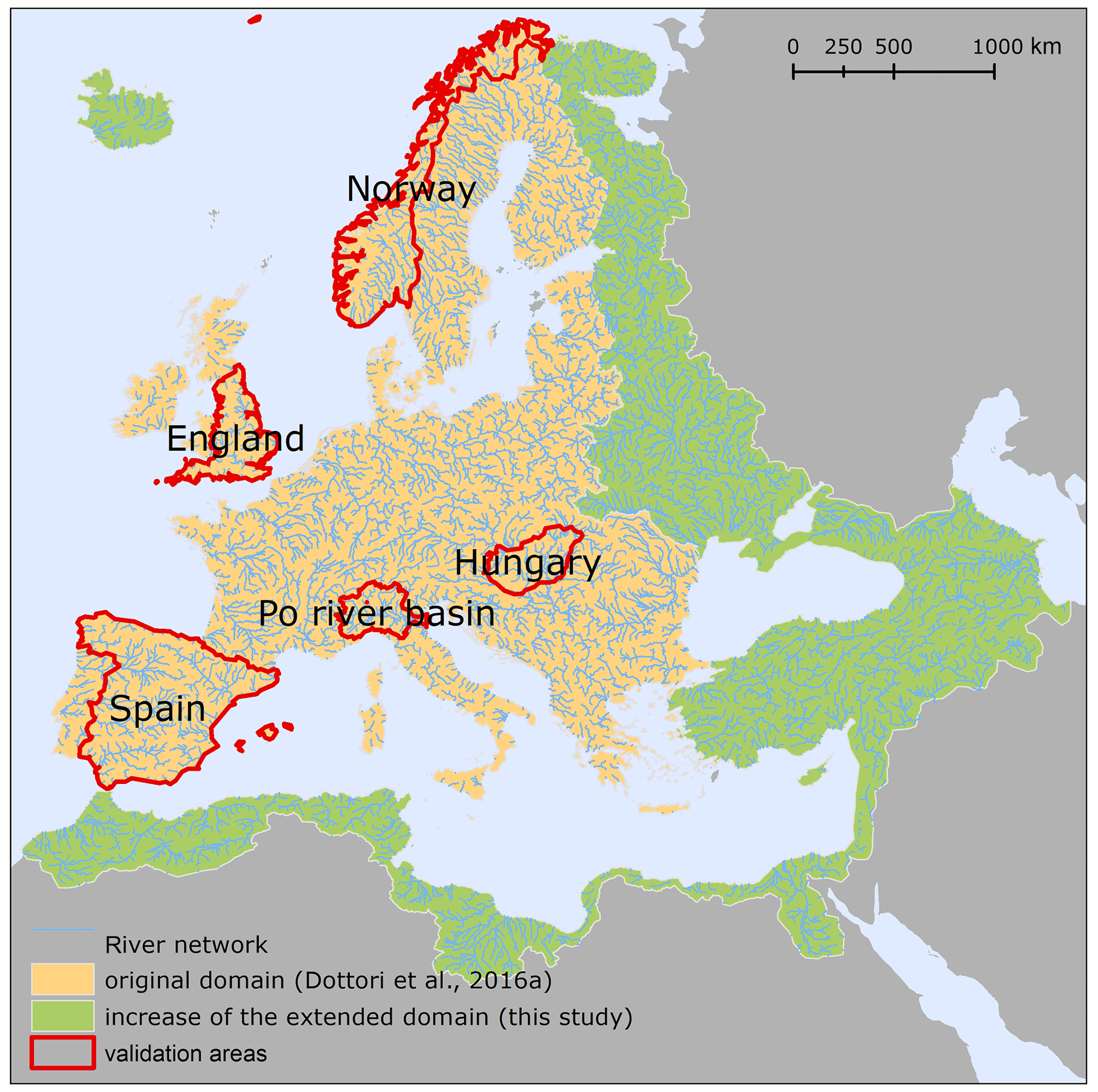
Figure 1Geographical extent of the EFAS extended domain covered by the present dataset of flood hazard maps. The extent of the map dataset produced by Dottori et al. (2016b) is depicted in beige, while the regions added with the extended domain are in green. The figure also displays the river network considered by the flood maps and the areas used for the validation exercise (see Sects. 2.3 and 3).
The current LISFLOOD version also benefits from an updated calibration at the European scale, based on the evolutionary-algorithm approach (Hirpa et al., 2018) with the modified Kling–Gupta efficiency criteria (KGE; Gupta et al., 2009) as an objective function and streamflow data for 1990–2016 from more than 700 gauge stations. The same stations have been used to validate model results, considering different periods of the time series. The calibration and validation procedure and the resulting hydrological skill are described by Arnal et al. (2019) and summarized in Appendix B. While we did not carry out a formal comparison with the previous LISFLOOD calibration, which used a different algorithm and performance indicators (Zajac et al., 2013), the larger dataset of streamflow observations and the improvement of the calibration routines should provide a better performance.
The geographical extent used in the present study to produce the flood maps follows the recent enlargement of EFAS (Arnal et al., 2019) and is shown in Fig. 1. The new domain is approximately 8 930 000 km2 wide (an increase of 76 % compared with the previous extent). The new extent covers the entire area of geographical Europe (with the exclusion of the Don River basin and Volga River basin and a number of river basins of the Arctic Sea in Russia); all the rivers entering the Mediterranean and Black Sea (with a partial inclusion of the Nile river basin); and all of the territories of Armenia, Georgia and Turkey and most of Syria and Azerbaijan.
The river network included in the new flood hazard maps has a total length of 329 000 km, with an 80 % increase compared with the previous flood maps (Alfieri et al., 2015; Dottori et al., 2016b).
2.2 Hydrological input of flood simulations
The hydrological input data required for the flood simulations are provided using synthetic flood hydrographs, following the approach proposed by Alfieri et al. (2014).
We use the streamflow dataset derived from the long-term run of LISFLOOD described in Sect. 2.1, considering the rivers with upstream drainage areas larger than 500 km2. This threshold was selected because the meteorological input data cannot accurately capture the short and intense rainfall storms that induce extreme floods in small river basins, and therefore the streamflow dataset does not represent accurately the flood statistics of smaller catchments (Alfieri et al., 2014).
For each pixel of the river network we selected annual maxima over the period 1990–2016, and we used the L-moments approach (linear combination of order statistics) to fit a Gumbel distribution and calculate peak flow values for reference return periods of 10, 20, 50, 100, 200 and 500 years. We also calculated the 30- and 1000-year return periods in limited parts of the model domain to allow for validation against official hazard maps (see Sect. 2.3). The resulting goodness of fit is presented and discussed in Appendix B. We used the Gumbel distribution to keep a parsimonious parameterization (two parameters instead of three for the generalized extreme-value (GEV) distribution, log-normal distribution and others), thus avoiding overparameterization when extracting high-return-period maps from a relatively short time series. The same distribution was also adopted for the extreme-value analysis in previous studies regarding flood frequency and hazard (Alfieri et al., 2014, 2015; Dottori et al., 2016a).
Subsequently, we calculate a flow duration curve (FDC) from the streamflow dataset. The FDC is obtained by sorting in decreasing order all the daily discharges, thus providing annual maximum values QD for any duration i between 1 and 365 d. Annual maximum values are then averaged over the entire period of data and used to calculate the ratios εi between each average maximum discharge for the ith duration QD(i) and the average annual peak flow (i.e. QD = 1 d). Such a procedure was carried out for all the pixels of the river network.
The synthetic flood hydrographs are derived using daily time steps, following the procedure proposed by Maione et al. (2003). The peak value of the hydrograph is given by the peak discharge for the selected T-year return period QT, while the other values for Qi are derived by multiplying QT by the ratio εi. The hydrograph peak QT is placed in the centre of the hydrograph, while the other values for Qi are sorted alternatively as shown in Fig. 2. The resulting hydrograph shape is therefore fully consistent with the empirical values of the flow duration curve. The total duration of the synthetic hydrograph is given by the local value of the time of concentration Tc such that all of the durations > Tc are discarded from the final hydrograph (Fig. 2).
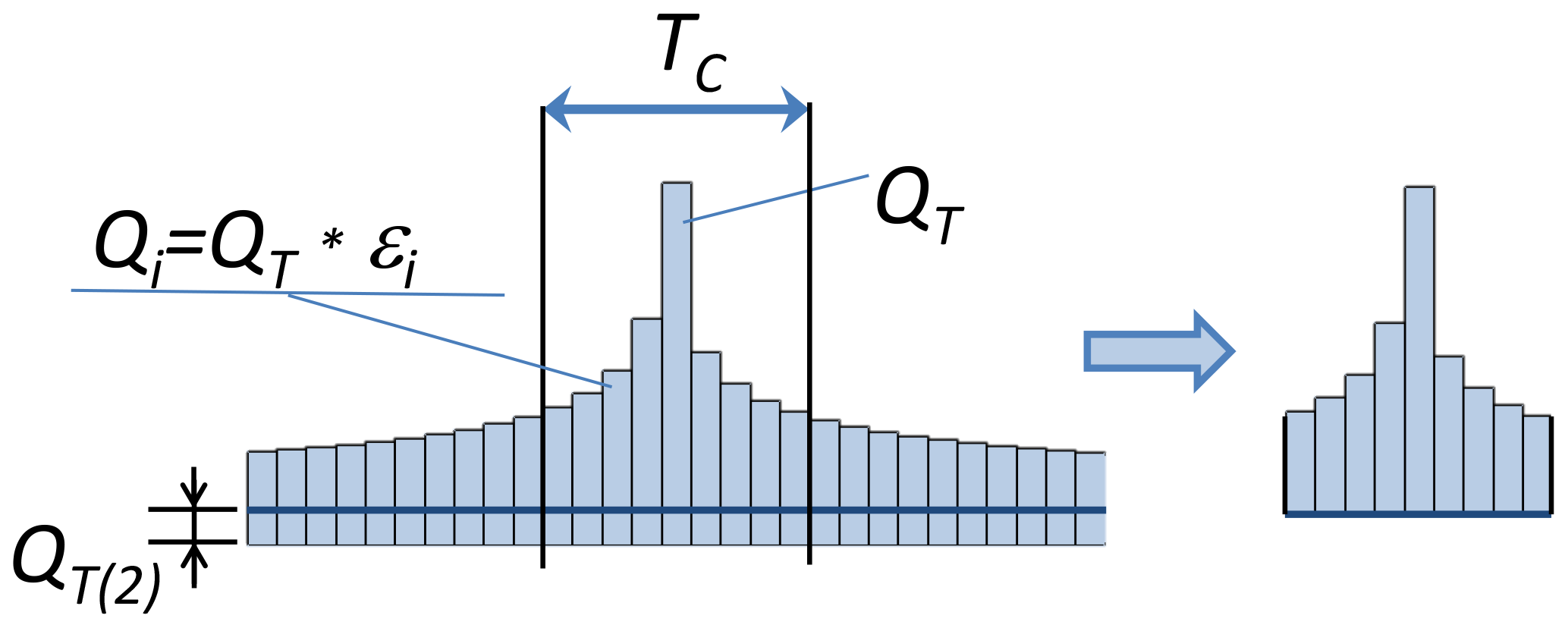
Figure 2General scheme of flood hydrographs (adapted from Alfieri et al., 2014).
Because river channels are usually not represented in continental-scale topography, flood hydrograph values are reduced by subtracting the 2-year discharge peak QT(2), which is commonly considered representative of full-bank conditions. (Note that the original DEM is not modified with this procedure.) Hence, the overall volume of the flood hydrograph is given by the sum of all daily flow values with a duration < Tc.
2.3 Flood hazard mapping
The continental-scale flood hazard maps are derived from local flood simulations run along the entire river network, as in Alfieri et al. (2014). We use the DEM at 100 m resolution developed for the Catchment Characterisation and Modelling database (CCM; Vogt et al., 2007) to derive a high-resolution river network at the same resolution. Along this river network we identify reference sections every 5 km along the stream-wise direction, and we link each section to the closest upstream section (pixel) of the EFAS 5 km river network, using a partially automated procedure to ensure a correct linkage near confluences. In this way, the hydrological variables necessary to build the flood hydrographs can be transferred from the 5 km to the 100 m river network. Figure 3 describes how the 5 km and 100 m river sections are linked using a conceptual scheme.
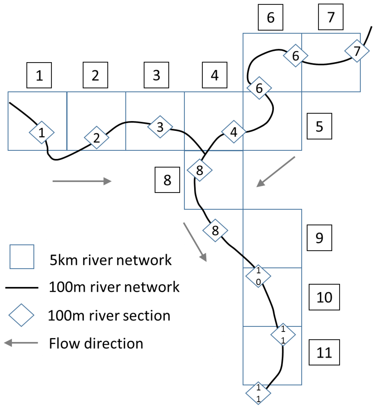
Figure 3Conceptual scheme of the EFAS river network (5 km, squares) with the high-resolution network (100 m) and river sections (diamonds) where flood simulations are derived. The related sections of the two networks are indicated by the same number. Source: Dottori et al. (2017).
Then, for every 100 m river section we run flood simulations using the two-dimensional hydrodynamic model LISFLOOD-FP (Shaw et al., 2021) to produce a local flood map for each of the six reference return periods. Simulations are based on the local inertia solver of LISFLOOD-FP developed by Bates et al. (2010), which is now available as open-source software (https://www.seamlesswave.com/LISFLOOD8.0, last access: 17 March 2022). We use the CCM DEM as elevation data, the synthetic hydrographs described in Sect. 2.2 as hydrological input data, and a mosaic of CORINE Land Cover for the year 2016 (Coordination of Information on the Environment; Copernicus Land Monitoring Service, 2017) and Copernicus GLOBCOVER (Global Land Cover map) for the year 2009 (Bontemps et al., 2011) to estimate the friction coefficient based on land use.
Finally, the flood maps with the same return period are merged together to obtain the continental-scale flood hazard maps. The 100 m river network is included as a separate map in the dataset to delineate those water courses that were considered in creating the flood hazard maps.
It is important to note that the flood maps developed do not account for the influence of local flood defences, in particular dyke systems. Such a limitation has been dictated mainly by the absence of consistent data at the European scale. None of the available DEMs for Europe has the required accuracy and resolution to embed artificial embankments into elevation data. Furthermore, there are no publicly available continental or national datasets describing the location and characteristics (e.g. dyke height and distance from river channel) for flood protections. Currently available datasets are based on the design return period of flood protection, e.g. the maximum return period of flood events that protections can withstand before being overrun (Jongman et al., 2014; Scussolini et al., 2016). Most of the protection standards reported by these datasets for Europe are based on empirical regressions derived using proxy variables (e.g. gross domestic product (GDP) and land use), with few data based on actual design standards. While these datasets have been applied to calculate flood risk scenarios (Alfieri et al., 2015) and flood impacts (Dottori et al., 2017), they have important limitations when used for mapping flood extent. Wing et al. (2017) linked the flood return period of protection standards with flood frequency analysis to adjust the bank height of the river channels, however with impaired performance of the model. Moreover, recent studies for the United States suggest that empirical regressions based on gross domestic product and land use may not be reliable (Wing et al., 2019b).
Despite these limitations, maps not accounting for physical flood defences may be applied to estimate the flood hazard in the case of failure of the protection structures and for flood events exceeding protection levels.
2.4 Validation of flood hazard maps
2.4.1 Selection of validation areas and maps
The validation of large-scale flood hazard maps requires the use of benchmarks with one or more datasets with extension and accuracy commensurate with the modelled maps. For instance Wing et al. (2017) used the official hazard maps developed for the conterminous United States to evaluate the performance of two flood hazard models designed to produce global- and continental-scale flood maps, respectively (see Sect. 1). In Europe, all EU member states as well as the UK have developed national datasets of flood hazard maps for a range of flood probabilities (usually expressed with the flood return period), following the guidelines of the EU Floods Directive (EC, 2007). These maps are usually derived using multiple hydrodynamic models of varying complexity (AdB Po, 2012) based on high-resolution topographic and hydrological datasets, such as DEMs of at least 5 m resolution in England (Sampson et al., 2015), lidar elevation data in Spain (MITECO, 2011) and river sections based on lidar surveys in the Po River basin (AdB Po, 2012). Although official maps might be either prone to errors or incomplete (Wing et al., 2017), these are likely to provide higher accuracy than the modelled maps presented here, and therefore they have been selected as reference maps for the validation. While official flood maps are generally available online for consultation on web GIS (geographic information systems) services, only a few countries and river basin authorities make the maps available for download in a format that allows for comparison with geospatial data. Table 1 presents the list of flood hazard maps that could be retrieved and used for the validation exercise, while their geographical distribution is shown in Fig. 1. Note that the relevant links to access these maps are provided in the Data availability section.
Table 1Characteristics of the flood hazard maps used in the validation exercise. The links for downloading the maps are provided in the Data availability section.
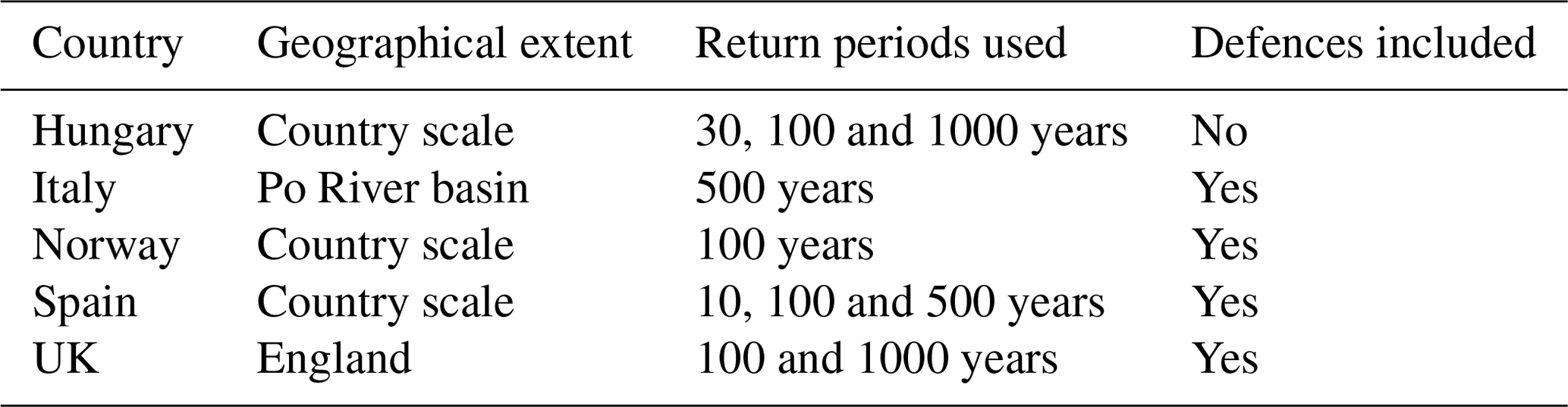
While more official maps like these are likely to become available in the near future, the maps considered here offer an acceptable overview of the different climatic zones and floodplain characteristics of the European continent. Conversely, we could not retrieve national or regional flood hazard maps outside Europe, meaning the skill of the modelled maps could not be tested in the arid regions of northern Africa and the eastern Mediterranean. In Norway, Spain, the UK and the Po River basin, the official maps take flood defences into account, which are not represented in the modelling framework. Official maps for England also include areas prone to coastal-flooding events (such as tidal and storm surges). None of the official maps include areas prone to pluvial flooding, which are therefore not considered in this analysis.
As mentioned in Sect. 2.3, the modelled maps do not include the effect of flood protections. Wherever possible, for the comparison exercise we selected either reference flood maps that do not account for protections (e.g. Hungary) or maps for flood return periods exceeding local protection standards, assuming that the resulting flood extent is relatively unaffected by flood defences. For example, the main stem of the Po River is protected against 1-in-200-year flood events (Wing et al., 2019b), whereas protection standards in England and Norway are usually above 20 years (Scussolini et al., 2016). Reference maps where the extent and design level of protection are not known (e.g. Spain) have been also included in the comparison to increase the number of validation areas.
2.4.2 Performance metrics and validation procedure
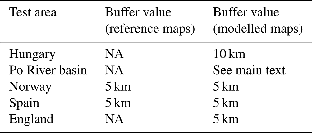
The national flood hazard maps listed in Table 1 are provided as polygons of flood extent, with no information on water depth or on the original resolution of data. According to Sampson et al. (2015), the official flood hazard maps for England are constructed using DEMs of at least 5 m resolution; therefore flood extent maps should be of comparable resolution. Reference flood maps for the Po basin and Spain are likely to have a similar resolution, since they are based on lidar elevation data (AdB Po, 2012; MITECO, 2011). For the comparison, official reference maps have been converted to raster format with the same resolution as the modelled maps (i.e. 100 m), while the latter have been converted to binary flood extent maps. To improve the comparison between modelled and reference maps, we applied a number of corrections. Firstly, we used the CORINE Land Cover map to exclude permanent waterbodies (river beds of large rivers or estuaries, lakes, reservoirs or coastal lagoons) from the comparison. Secondly, we restricted the comparison area around modelled maps to exclude the elements of a river network (e.g. minor tributaries) included in the reference maps but not in the modelled maps. We used a different buffer extent according to each study area, considering the floodplain morphology and the variable extent and density of mapped river network. For example, in Hungary we applied a 10 km buffer around modelled maps to include the large flooded areas reported in reference maps and to avoid overfitting. In England, we used a 5 km buffer due to the high density of the river network mapped in the official maps. The buffer is also applied to mask out coastal areas far from rivers estuaries because official maps include flood-prone areas due to 1-in-200-year coastal flood events. We calculated that flood-prone areas inside the 5 km buffer correspond to 73 % of the total extent for the 1-in-100-year flood. For the Po River basin, we excluded from the comparison the areas belonging to the Adige River basin and the lowland drainage network, which are not included in the official hazard maps. In Spain and Norway official flood hazard maps have only been produced where relevant assets are at risk, according to available documentation (MITECO 2011; NVE, 2020). We therefore restricted the comparison only to areas where official flood hazard maps have been produced. Table 2 provides the list of parameters used to determine the areas used for the comparison.
Table 2List of parameters used to determine the extent of areas used for comparing reference and modelled maps (NA: buffer not applied).
We evaluate the performance of simulated flood maps against reference maps using a number of indices proposed in the literature (Bates and De Roo, 2000; Alfieri et al., 2014; Dottori et al., 2016a; Wing et al., 2017). The hit rate (HR) evaluates the agreement of simulated maps with observations and it is defined as
where Fm∩Fo is the area correctly predicted as flooded by the model and Fo indicates the total observed flooded area. HR scores range from 0 to 1, with a score of 1 indicating that all wet cells in the benchmark data are wet in the model data. The formulation of the HR does not penalize overprediction, which can be instead quantified using the false-alarm rate FAR:
where is the area wrongly predicted as flooded by the model. FAR scores range from 0 (no false alarms) to 1 (all false alarms). Finally, a more comprehensive measure of the agreement between simulations and observations is given by the critical-success index (CSI), defined as
where Fm∪Fo is the union of observed and simulated flooded areas. CSI scores range from 0 (no match between model and benchmark) to 1 (perfect match between benchmark and model).
2.5 Additional tests
To choose the best possible methodologies and datasets to construct the flood hazard maps, we performed a number of tests using recent input datasets, as well as alternative strategies to account for vegetation effects on elevation data.
2.5.1 Elevation data
It is well recognized that the quality of flood hazard maps strongly depends on the accuracy of elevation data used for modelling (Yamazaki et al., 2017). This is especially crucial for continental-scale maps, since the quality of available elevation datasets is rarely commensurate with the accuracy required for modelling flood processes (Wing et al., 2017). Moreover, high-resolution and accurate elevation data such as lidar-based DEMs cannot be used for reasons of consistency, since these data are only available for few areas and countries.
The recent release of new global elevation models have the potential to improve the accuracy of large-scale flood simulations and hence the quality of flood hazard maps. Here, we test the use of the MERIT DEM (Multi-Error-Removed Improved-Terrain; Yamazaki et al., 2017) within the proposed modelling approach, and we compare the results with those obtained with the CCM DEM. The MERIT DEM is based on the Shuttle Radar Topography Mission (SRTM) data, similar to the CCM DEM, but has been extensively corrected and improved through comparisons with other large-scale datasets to eliminate error bias, improve data accuracy at high latitudes (areas above 60∘ are not covered by SRTM) and compensate for factors like vegetation cover. Note that areas above 60∘ in the CCM DEM were derived from national datasets, and therefore these areas are where the two datasets are likely to differ most.
2.5.2 Correction of elevation data with land use
The CCM DEM elevation dataset is mostly based on SRTM data, and so the elevation values can be spuriously increased by the effect of the vegetation canopy in densely vegetated areas and by buildings in urban areas. Recent research work has proposed advanced techniques to remove surface artefacts, based on artificial neural networks (Wendi et al., 2016; Kulp and Strauss, 2018) or other machine learning methods (Liu et al., 2019; Meadows and Wilson, 2021). Most approaches correct DEM elevation with higher-accuracy datasets, using auxiliary data such as tree density and height for correcting vegetation bias (as done for the MERIT DEM by Yamazaki et al., 2017), whereas elevation bias in urban areas can be corrected using night light, population density or OpenStreetMap elevation data (Liu et al., 2019). Given that improving elevation data is not the main scope of this work, we opted for applying a simpler method for quickly correcting the CCM DEM elevation data. Specifically, we use the land cover map derived from CORINE Land Cover and Copernicus GLOBCOVER to identify densely vegetated areas and urban areas, and we applied a correction factor as a function of local land use to reduce elevation locally. The correction factor varies from 8 m for densely forested areas to 2 m for urban areas. Note that these values are based on the findings of previous literature studies such as Baugh et al. (2013) and Dottori et al. (2016a), while a formal calibration was not undertaken.
We present the outcomes of the validation exercise by first describing the general results at the country and regional scale (Sect. 3.1). Then, we discuss the outcomes for England, Hungary and Spain (Sect. 3.2), while the Norway and Po River basin case studies are presented in Appendix C. We also complement the analysis with additional validation over major river basins in England and Spain. In Sect. 3.3 we compare our results with the validation exercise carried out by Wing et al. (2017) and with the findings of other literature studies. Finally, in Sect. 3.4 and 3.5 (and Appendix B) we compare the performance of the present and previous versions of the flood hazard map dataset, and we discuss the results of the tests with different elevation data and strategies to account for vegetation.
3.1 Validation of modelled maps at the national and regional scale
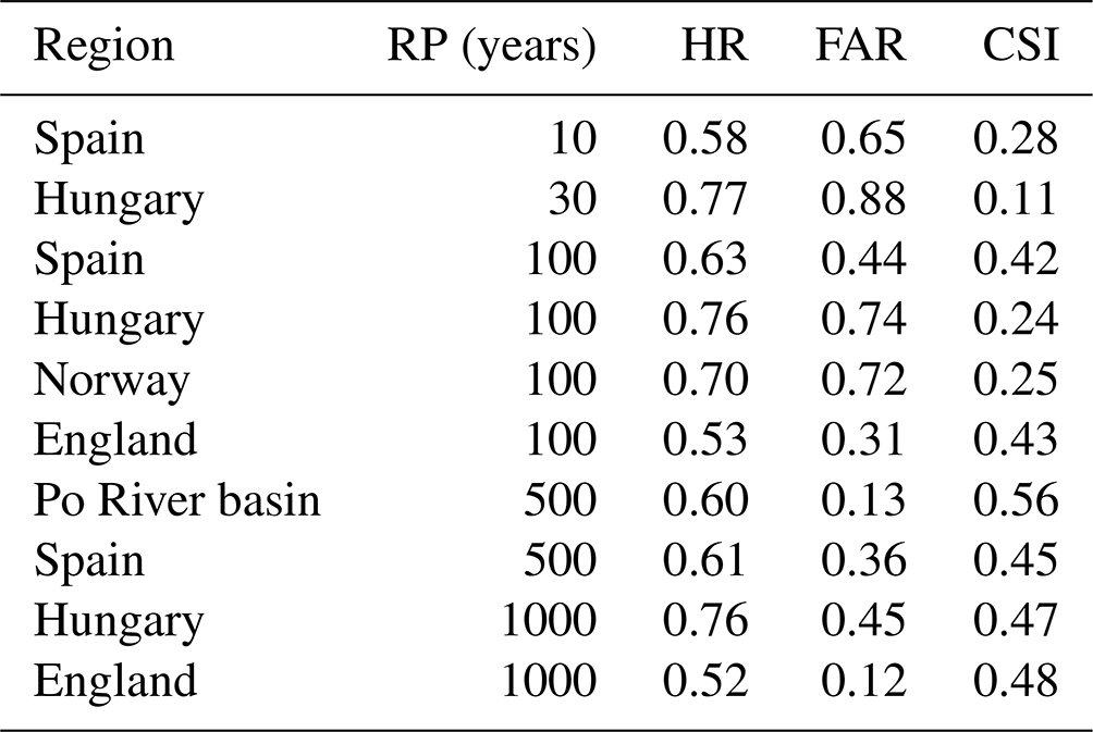
Table 3 presents the validation results for each testing area and return period. The performance metrics are calculated using the total extent of the reference and modelled maps with the same return period. The first visible outcome is the low scores for the comparisons with reference maps with a high probability of flooding, i.e. low flood return periods (< 30 years). Performances improve markedly with the increase of return periods due to the decrease of the false-alarm rate (FAR), while the hit rate (HR) does not vary significantly. In particular, critical-success index (CSI) values approach 0.5 for the low-probability flood maps, i.e. for return periods equal or above 500 years. Considering that most of the reference flood maps include the effect of flood defences (unlike the modelled maps), these results suggest that the majority of rivers in the study areas may be protected for flood return periods of around 100 years or less, as indeed reported by available flood defence databases (Scussolini et al., 2016). Differences between simulated and reference hydrological input are likely to influence the skill of modelled flood maps and may depend on several factors such as the hydrological-model performance for peak flows, the extreme-value analysis (distribution used for extreme-value fitting and length of available time series) and the design hydrograph estimation. In the following sections, we evaluate the modelled hydrological regime considering the skill of the LISFLOOD long-term simulation and the uncertainty of the extreme-value analysis (see Appendix B2). However, further analysis is difficult, as we have no specific information on the hydrological input used for the reference flood maps (e.g. peak flows, statistical modelling of extremes and hydrograph shape). High-probability floods are also sensitive to the method used to reproduce river channels, and the simplified approach used in this study might underestimate the conveyance capacity of channels (see Sect. 3.2.2 for an example). Finally, the better performance for low-probability floods may also depend on floodplain morphology, where valley sides create a morphological limit to flood extent.
Table 3Results of the validation against official flood hazard maps. Value of the performance indices at country and regional scale. RP: return period, HR: hit rate, FAR: false-alarm rate, CSI: critical-success index.
3.2 Discussion of results at the national and regional scale
The results in Table 3 highlight considerable differences in the skill of the flood maps across countries and regions. While some differences may arise from the variability of floodplain morphology and model input data, others are attributable to the different methods applied to produce the reference maps (MITECO, 2011; NVE, 2020). In the following sections we examine in more detail the outcomes for each study area.
3.2.1 England
According to Table 3, modelled flood maps tend to underestimate flood extent in England, as visible by the HR values around 0.5 (e.g. out of every two flooded cells, only one is correctly identified as flooded by the model). Such a result is confirmed when focusing the analysis on the major river basins of England, as reported in Table 4. Notably, HR has generally marginal or no increases with the increase of the return period considered, while FAR values have a marked decrease. Results reported by Arnal et al. (2019) and summarized in Fig. B1 suggest a fair hydrological skill of the LISFLOOD calibration in England, with KGE values generally above 0.5. The difference between estimated and reference discharge annual maxima is also acceptable, generally below 25 %. However, there is not a clear correlation between hydrological and flood map skill, with some basins (e.g. Thames) showing high KGE values but relatively low CSI values.
Table 4Validation indices in England and in major river basins.

For the Thames basin, the low CSI value is likely influenced by the tidal flooding component from London eastwards. According to Sampson et al. (2015), the official flood hazard map assumes a 1-in-200-year coastal flood along with the failure of the Thames tidal barrier, whereas our river flood simulations use the mean sea level as a boundary condition and do include storm surge and tidal flooding. Concurrent fluvial–tidal flooding processes occur in other river estuaries, so this might reduce the skill of the modelled maps. Furthermore, the Thames catchment is heavily urbanized and has extensive flood defence and alleviation schemes compared to the other catchments (Sampson et al., 2015). Both aspects might increase the elevation bias of the CCM DEM and complicate the correct simulation of extreme flood events.
Besides these results, the visual inspection of reference maps suggest that the underestimation is partly caused by the high density of mapped river network in the reference maps, with respect to modelled maps. Indeed, the modelling framework excludes river basins with an upstream basin area below 500 km2, meaning that EFAS maps only cover main river stems but miss several smaller tributaries. This is clearly visible over the Severn and in the upper Thames basins (Fig. 4) and might also explain the lower skill in the lowlands of Ouse and Trent rivers, where the contributions of main river stems and tributaries to the flood extent are difficult to separate. Including minor tributaries in the flood maps would require either increasing the resolution of the climatological forcing to reproduce intense local rainfall or adding a pluvial flooding component as done by Wing et al. (2017). Finally, areas prone to storm surge and tidal flooding around river estuaries might further reduce the overall skill of modelled maps, despite the 5 km buffer applied.
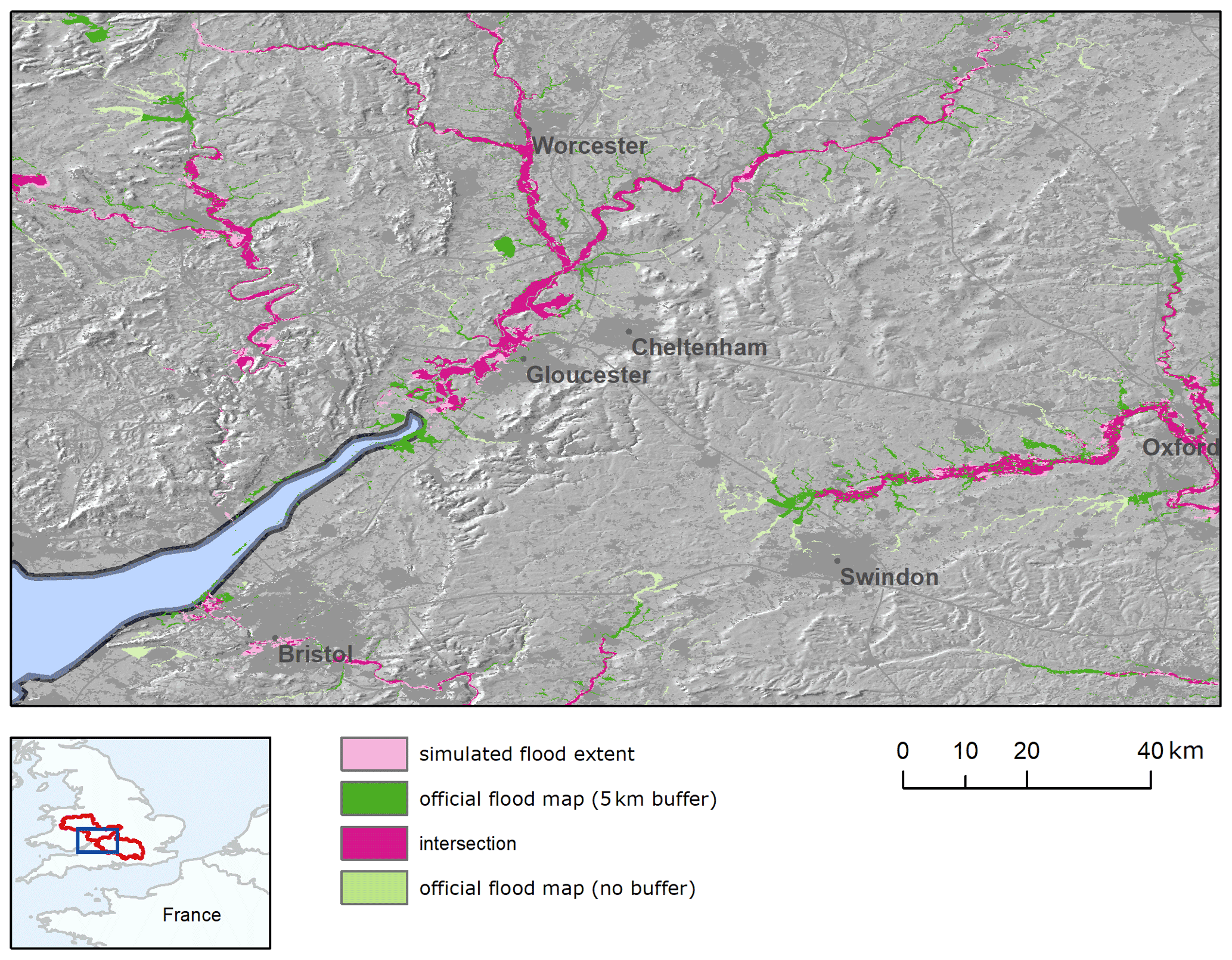
Figure 4Comparison of modelled (blue) and reference (green) flood hazard maps (1-in-100-year flood hazard) over the Severn (centre) and the upper Thames (right) river basins in England. Purple areas denote the intersection (agreement) between the modelled and reference set of maps. The original reference maps (i.e. with no masking around modelled maps) are shown in light green.
3.2.2 Hungary
The results in Table 3 for Hungary show a general tendency to overestimate flood extent for all return periods. HR values are consistently high and do not change much with the return period. Conversely, FAR is very high for the 1-in-30-year flood map and still considerable even for the 1-in-1000-year flood map. Arnal et al. (2019) reported a fair hydrological skill of LISFLOOD (KGE values > 0.5) for the calibration period, even though KGE validation values were considerably low for the Tisza River. The uncertainty of estimated discharge annual maxima is also comparable to the average values reported in Appendix B2.
Given that flood defences are not modelled in reference maps, the observed results may be explained by assuming a large conveyance capacity of river channels. For instance, the 1-in-100-year reference map shows relatively few flooded areas for the Danube main stem (Fig. 5), thus suggesting that the main channels can convey the 1-in-100-year discharge without overflowing. Conversely, river channels in the modelling framework are assumed to convey only the 1-in-2-year discharge. Obviously, the same considerations can be made for 1-in-30-year discharge for the majority of river network, which explains the very low scores. Furthermore, artificial structures such as road embankments and drainage networks may further reduce flood extent in lowland areas, leading to a further overestimation given the fact that these features are not represented in the DEM. These findings highlight the need for a high-resolution DEM fed with local-scale information to achieve adequate performance in lowland areas, as observed also by Wing et al. (2019b).
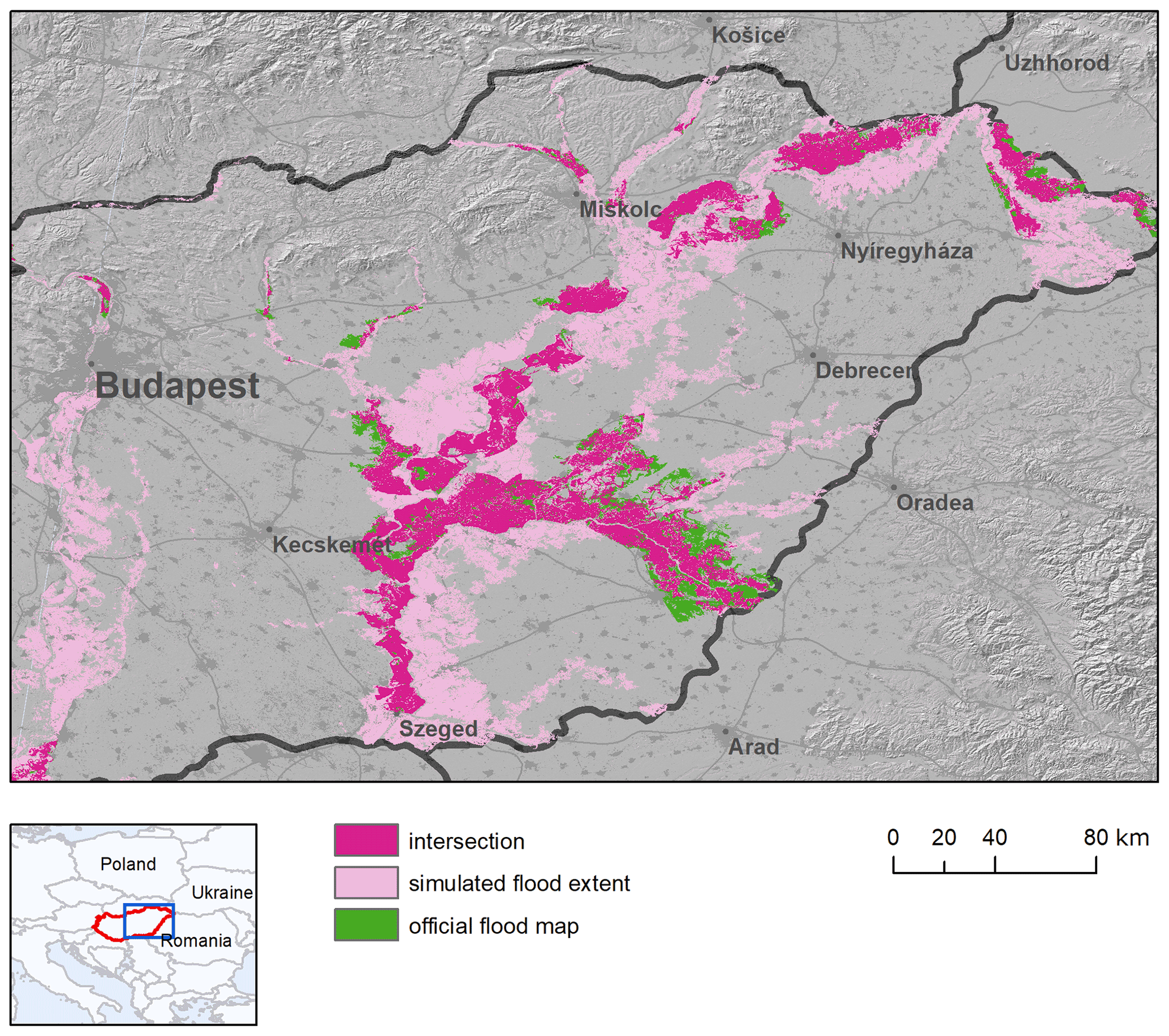
Figure 5Comparison of modelled (blue) and reference (green) flood hazard maps (1-in-100-year flood hazard) over the Danube (left) and Tisza (right) rivers in Hungary. Purple areas denote the intersection between the modelled and reference set of maps.
3.2.3 Spain
The performance of the modelled maps in Spain shows a fairly stable HR value and decreasing FAR values with increasing return periods, similarly to what was observed for England and Hungary. The analysis of the results for the major river basins of the Iberian Peninsula, reported in Table 5, provide further insight into the skill of flood maps. A number of basins exhibit both large HR and FAR such as the Douro, Tagus and Guadalquivir basins. Rivers in south-eastern Spain (Segura and Júcar) have relatively low HR values, while the modelled maps perform better in the Ebro river basin. The interpretation of results requires the consideration of different aspects. The poor results for the 1-in-10-year maps are likely due to the effect of flood protection structures, such as dykes and flood regulation systems, which are probably relevant also for the 1-in-100-year map. Indeed, most Iberian rivers are regulated by multiple reservoirs, which are often used to reduce flood peaks according to specific operating rules. While dykes are not represented in the inundation model, reservoirs are included in the LISFLOOD model through a simplified approach, given that operating rules are not known. Therefore, the real and modelled hydrological regimes might differ significantly, including flow peaks of low-probability flood events. This is also reflected by the low hydrological skill of LISFLOOD, with KGE values generally below 0.5 with few exceptions (Fig. B1).
Table 5Validation indices in Spain and in some test river basins.
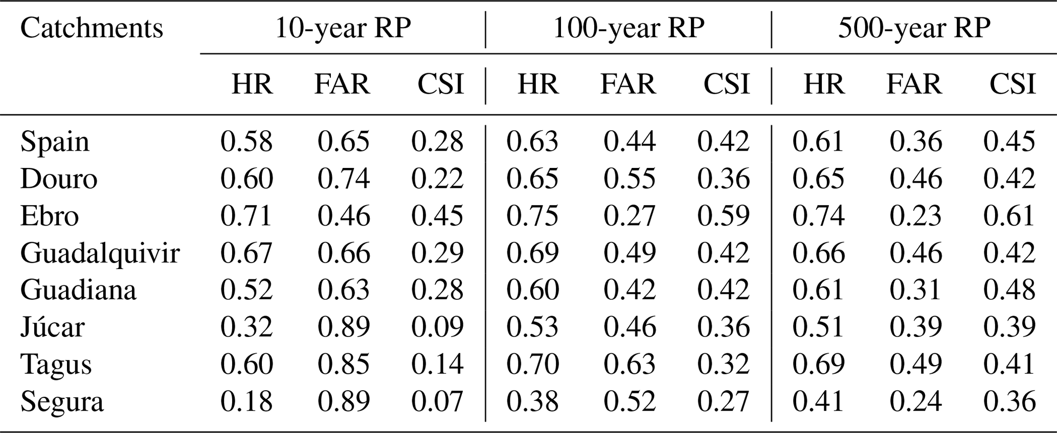
In addition, the comparison of modelled and reference maps is affected by the partial coverage of the reference inundation maps in several river basins. According to the information available on the official website (MITECO, 2011) large sections of the river network in the basins of the Douro, Tagus, Guadiana and Guadalquivir rivers have not been analysed, due to the absence of relevant assets or inhabited places at risk. Even though this has been accounted for by restricting the area of comparison around reference maps, a visual inspection of the maps being compared shows spurious overestimation around the edges of reference map polygons (Fig. 6). Finally, the low HR values scored in rivers in south-eastern Spain (Segura and Júcar) are partially explained by the presence of several tributaries not included in EFAS maps.

Figure 6Comparison of modelled (blue) and reference (green) flood hazard maps (1-in-100-year flood hazard) over a stretch of the Guadalquivir river basin, Spain. Purple areas denote the intersection between the two sets of maps.
3.3 Comparison with previous continental-scale validation studies
To put the previously described results into context, we compare them with the validation exercises performed by Sampson et al. (2015) over the Thames and Severn rivers in England and by Wing et al. (2017) over the United States. The study by Wing et al. (2017) is, to our knowledge, the first study that carried out a consistent validation of modelled flood hazard maps at the continental scale. Bates et al. (2021) have recently updated the work by Wing et al. (2017), by including pluvial and coastal-flooding components in the modelling framework, but their work is not considered here. A comparison of validation metrics of the three studies is shown in Tables 6 and 7. For our framework, we calculated each index in Table 6 using the overall modelled and reference flood extent available for each return period (e.g. the value for the 100-year maps includes reference and modelled maps for England, Spain and Norway). As such, each area is weighted according to the extent of the corresponding flood map.
Table 6Comparison of the performance metrics for the European model described in the present study and the two models evaluated in the study by Wing et al. (2017). NA – not available
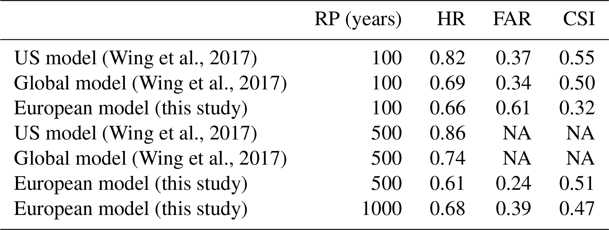
Table 7Comparison of the performance metrics for the maps described in the present study and the global maps by Sampson et al. (2015). Metrics for the latter study are calculated removing all channels with upstream areas of less than 500 km2.

As can be seen in Table 6, the continental-scale model by Wing et al. (2017), achieved the highest scores both for 100- and 500-year return periods. However, this model is based on national datasets with higher accuracy and resolution than those available for the European continent (e.g. a 10 m resolution DEM and a detailed catalogue of flood defences). The global and European models have comparable hit rates for the 100-year flood maps (0.68 and 0.65, respectively), but the former exhibits a much lower FAR value (0.34 compared to 0.61 for the European model) and a higher HR value for the 500-year maps.
The higher HR values scored by the US and global models might depend on the higher density of the modelled river network, which includes river reaches up to 50 km2 by simulating both pluvial and fluvial flooding processes. The lower FAR values of the US and global models might be explained by the inclusion of flood defences. In the US model, defences are explicitly modelled using the US dataset of flood defences, while the global model parameterizes flood defences through the adjustment of channel conveyance using socioeconomic factors and the degree of urbanization (Wing et al., 2017). However, Wing et al. (2017), observed that the latter methodology had a negligible effect on HR values in defended areas, when compared with an undefended version of the model.
Another possible reason for the low FAR values is the different approach used in the validation method. Wing et al. (2017), applied a narrow 1 km buffer around official maps to constrain the area of comparison and avoid spurious overprediction in areas not considered by official maps. However, this might result in a reduction of true false alarms because part of the overestimated flood areas can go undetected. To verify this hypothesis, we recalculated the performance indices against the 100-year reference map in Spain using a 1 km buffer instead of the 5 km one previously applied to constrain the validation area. As a result the FAR value dropped from 0.44 to 0.34, similar to the performance of the global model. However, we observed a reduction of true false alarms, especially in river basins with continuous map coverage such as the Ebro, Júcar and Segura.
The comparison of HR, FAR and CSI values shows better scores for the global maps by Sampson et al. (2015) with respect to our modelled maps (Table 7).
The different masking applied to reference flood maps may explain some of the differences: Sampson et al. (2015) removed all channels with upstream areas of less than 500 km2, whereas here we use a simpler 5 km buffer around modelled maps. The exclusion of permanent river channels in our comparison may further penalize the overall score especially for the Thames, which as a rather large channel estuary. Besides these differences in the validation, the better metrics of the maps by Sampson et al. (2015) may depend on a more accurate hydrological input (based on the regionalization of gauge station data) and a better correction of urban elevation bias (based on a moving-window filter instead of the constant correction values applied here).
To provide further context, the US model by Wing et al. (2017) attained average CSI values of ∼ 0.75 against a number of detailed local models, whereas flood models built and calibrated for local applications may achieve CSI scores up to 0.9 when benchmarked against very high-quality data (see Wing et al., 2019a). Fleischmann et al. (2019) recently proposed that regional-scale models can provide locally relevant estimates of flood extent when CSI > 0.65. Although the overall values shown in Table 3 are consistently below this threshold, better results are observed for a number of river basins, as shown in Tables 4 and 5.
3.4 Comparison with the previous flood map dataset
Table 8 compares the performances of the flood hazard maps described in the present study (version 2) with the previous version developed by Dottori et al. (2016b; version 1). The comparison is shown for England and Hungary. Results for all other areas are comprised within the range of results shown in Table 3. As can be seen, differences are generally reduced across the different areas and return periods. Version 1 of the flood maps produced slightly better results in Hungary for the 100- and 1000-year return period (increased CSI and HR and lower FAR), while version 2 has somewhat improved performances in England, mainly driven by higher HR.
Table 8Comparison of performances of the flood hazard maps described in the present study and developed by Dottori et al. (2016b). Table reports the ratio between flood extents (F2 / F1) and the difference between version 2 and 1 of the HR, FAR and CSI values.
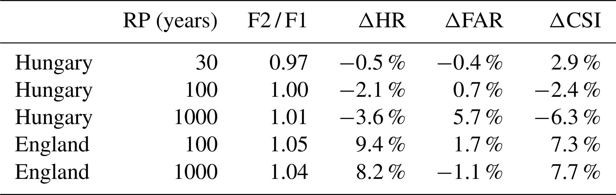
These outcomes may be interpreted considering the changes in input data between the two versions and the structure of the modelling approach and of input data, which in turn has not changed substantially. The main difference between the two map versions is given by the hydrological input, with version 2 using the latest calibrated version of the LISFLOOD model.
For the 100-year return period, peak flow values of version 2 are on average 35 % lower than version 1 in Hungary and 16 % lower in England. However, similar decreases are also observed for the 1-in-2-year peak discharge that determines full-bank discharge. The resulting reduction in channel hydraulic conveyance with respect to version 1 is likely to offset the decrease of peak flood volumes, which explain the small difference in overall flood extent given by the F2 / F1 parameter in Table 8. Such results confirm the low sensitivity of the modelling framework to the hydrological input observed by Dottori et al. (2016a) and by Trigg et al. (2016) for a global-scale application. This low sensitivity is likely to offset the uncertainty related to the estimation of peak flow values reported in Appendix B. The results also confirm that the knowledge of river channel geometry is crucial to correctly model the actual channel conveyance and thus improve inundation modelling. Other differences in input data are given by minor changes in Manning's parameters and in the EFAS river network, which might contribute to the observed differences.
3.5 Influence of elevation data
Table 9 compares the metrics calculated with the CCM DEM elevation data against the same metrics for the modelled flood maps based on the MERIT DEM. The comparison is carried out for England, Hungary and the Po River basin. Performance is slightly improved by the use of MERIT DEM data for all areas and return periods, in particular through the reduction of FAR, even though the overall increase of CSI values is limited to a few percentage points.
Table 9Comparison of performances of the flood hazard maps described in the present study and developed by Dottori et al. (2016b) based on the MERIT DEM (a) and the CCM DEM (b). Table reports the ratio between flood extents F and the differences for HR, FAR and CSI (e.g. ().
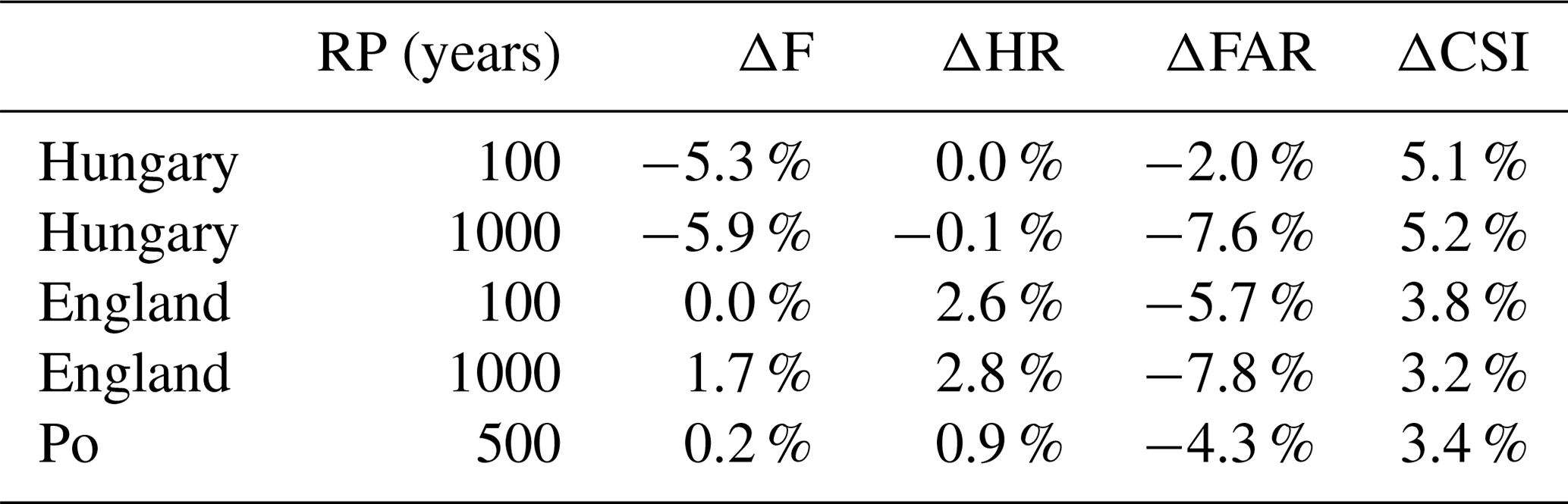
Because of this limited improvement and the considerable amount of time required to re-run the complete set of flood hazard maps (several days for each return period), it was decided not to update the flood maps using the MERIT DEM as elevation data. Moreover, new high-resolution datasets such as the Copernicus DEM (ESA-Airbus, 2019), the 90 m version of the TanDEM-X (TerraSAR-X – synthetic-aperture radar – add-on for Digital Elevation Measurements) dataset (https://geoservice.dlr.de/web/dataguide/tdm90, last access: 17 March 2022) and MERIT Hydro (Yamazaki et al., 2019) have recently become available, and therefore future research could focus on performing additional comparisons to identify which dataset is most suitable for inundation modelling in Europe.
We presented here a new dataset of flood hazard maps covering geographical Europe and including large parts of the Middle East and river basins entering the Mediterranean Sea. This dataset significantly expands the previous available flood maps datasets at the continental scale (Alfieri et al., 2014; Dottori et al., 2016b) and therefore constitutes a valuable source of information for future research studies and flood management, especially for countries where no official flood hazard maps are available. The new maps also benefit from updated models and new calibration and meteorological data. The maps are being used for a range of applications at the continental scale, from evaluating present and future river flood risk scenarios to the cost–benefit assessment of different adaptation strategies to reduce flood impacts, and for comparisons between different regions, countries and river basins (Dottori et al., 2020b). Moreover, the flood hazard maps are designed to be integrated with the Copernicus European Flood Awareness System (EFAS) and will be used to perform operational flood impact forecasting in EFAS (Dottori et al., 2017).
We performed a detailed validation of the modelled flood maps in several European countries against official flood hazard maps. The resulting validation exercise is the most complete undertaken so far for Europe to our best knowledge and provided a comprehensive overview of the strengths and limitations of the new maps. Nevertheless, the unavailability of reference flood maps outside Europe did not allow for any validation in the arid regions in northern Africa and the eastern Mediterranean. In these areas, further research will be needed to better understand the performance of the flood mapping procedure here proposed. Modelled maps generally achieve low scores for a high and medium probability of flooding. For the 1-in-100-year return period, the modelled maps can identify on average two-thirds of reference flood extent; however they also largely overestimate flood-prone areas in many regions, thus hampering the overall performance. Performances improve markedly with the increase of the return period, mostly due to the decrease of the false-alarm rate. In particular, critical-success index (CSI) values approach and in some cases exceed 0.5 for return periods equal to or above 500 years, meaning that the maps can correctly identify more than half of flooded areas in the main river stems and tributaries of different river basins.
It is important to note that the validation was affected by problems in identifying the correct areas for a fair comparison because of the different density of the mapped river network in reference and modelled maps. In our study we used large buffers to constrain comparison areas, which possibly penalized the model performance by generating spurious false alarms in areas not considered by official maps. However, we observed that the proposed maps achieve results comparable to other large-scale flood models when using similar parameters for the validation.
The low skill of modelled maps for a high and medium probability of flooding, with large overestimations observed in different lowland areas, is likely motivated by the non-inclusion of flood defences in the modelling framework and the simplified representation of channel hydraulic conveyance, due to the absence of datasets at the European scale describing river channels and defence structures (i.e. design standards and the location of dyke systems). Such information combined with a high-resolution DEM fed with local-scale information (artificial and defence structures) is crucial to improve the performance of large-scale flood models and apply more realistic flood modelling tools, as observed also by Wing et al. (2017, 2019b). Uncertainty in peak flow estimation can also influence the skill of the modelled maps; however, we found that the limited sensitivity of the modelling approach to changes in the hydrological input smooths out this uncertainty source because channel conveyance is linked to streamflow characteristics. Such findings highlight the need for independent data of river channel width, shape and depth to better reproduce streamflow and flooding processes. Moreover, the improved results offered by the use of the MERIT DEM elevation data suggest that recent high-resolution datasets such as the Copernicus DEM (ESA-Airbus, 2019), TanDEM-X (https://geoservice.dlr.de/web/dataguide/tdm90, last access: 17 March 2022) and MERIT Hydro (Yamazaki et al., 2019) may offer a viable solution to improve future versions of continental-scale flood hazard maps in Europe.
Increasing map coverage by including the minor river network is likely to improve the skill of modelled maps. However, this might require the use of a different modelling approach to account for pluvial flooding (Wing et al., 2017; Bates et al., 2021), along with reliable model climatology to represent small-scale precipitation processes. Improving the simulation of reservoirs may also reduce the difference between the real and modelled hydrological regimes in regions such as the Iberian Peninsula and the Alps.
The dataset described in this paper is accessible as part of the data collection “River Flood Hazard Maps at European and Global Scale” at the Joint Research Centre (JRC) Data Catalogue (https://doi.org/10.2905/1D128B6C-A4EE-4858-9E34-6210707F3C81, Dottori et al., 2020a).
The dataset comprises the following maps (eight in total), each one available as a raster (GeoTIFF) file:
-
map of permanent waterbodies for Europe and the Mediterranean basin
-
river network in Europe and the Mediterranean basin
-
river flood hazard maps for Europe and the Mediterranean basin (return periods of 10, 20, 50, 100, 200 and 500 years).
The official flood hazard maps used for the validation exercise are freely accessible at the following websites.
-
Spain: https://www.miteco.gob.es/es/cartografia-y-sig/ide/descargas/agua/zi-lamina.aspx (Ministerio para la Transición Ecológica y el Reto Demográfico, 2022) (in Spanish)
-
Po River basin: https://pianoalluvioni.adbpo.it/mappe-del-rischio-2/download-mappe/ (Autorità di bacino distrettuale del fiume Po, 2022) (in Italian)
-
Norway: https://www.nve.no/flaum-og-skred/kartlegging/flaum/ (Noregs Vassdrags- og Energidirektorat, 2022) (in Norwegian)
-
England: https://data.gov.uk/dataset/bed63fc1-dd26-4685-b143-2941088923b3/flood-map-for-planning-rivers-and-sea-flood-zone-3 (Environment Agency, 2022a) https://data.gov.uk/dataset/cf494c44-05cd-4060-a029-35937970c9c6/flood-map-for-planning-rivers-and-sea-flood-zone-2 (Environment Agency, 2022b) (in English)
-
Hungary: https://www.vizugy.hu/index.php?module=content&programelemid=62 (Országos Vízügyi Főigazgatóság, 2022) (in Hungarian)
The LISFLOOD hydrological model used in this research is released as open-source software and available at https://ec-jrc.github.io/lisflood/ (European Commission JRC, 2022).
The streamflow dataset derived from the long-term run of the LISFLOOD model is available at https://cds.climate.copernicus.eu/cdsapp#!/dataset/efas-historical (Copernicus Climate Change Service, 2022).
The LISFLOOD-FP hydrodynamic model used in this research is available as open-source software at https://www.seamlesswave.com/LISFLOOD8.0 (University of Bristol, 2022) for research and non-commercial purposes.
The MERIT-DEM dataset used in this research is available at http://hydro.iis.u-tokyo.ac.jp/~yamadai/MERIT_DEM (Yamazaki et al., 2018).
The CCM DEM dataset used in this research is not publicly available due to the use of proprietary data. The dataset can be requested for research purposes upon reasonable request.
All links were accessed on 14 February 2022.
The long-term run of the hydrological model LISFLOOD is based on observed data from meteorological stations and precipitation datasets, which are collected and continuously expanded as part of the development work for EFAS. The meteorological variables considered are precipitation, minimum and maximum temperature, wind speed, solar radiation, and vapour pressure. The number of stations with available meteorological observations depends on the period and variable considered, with an increasing availability towards the end of the historical simulation period. As an example, for the year 2016 the number of daily observations available ranged from ∼ 8800 for temperature to ∼ 5500 for precipitation and ∼ 3700 for vapour pressure. The input from meteorological stations is completed by a number of precipitation datasets (EURO4M-APG, EUropean Reanalysis and Observations for Monitoring–Alpine precipitation grid dataset; INCA-Analysis Austria, Integrated Nowcasting through Comprehensive Analysis; ERA-Interim GPCP corrected, European Centre for Medium-Range Weather Forecasts Reanalysis and Global Precipitation Climatology Project; and CARPATCLIM, Climate of the Carpathian Region; for details, see Arnal et al., 2019). Note that the same datasets are used to drive the LISFLOOD calibration and to calculate the initial conditions for the EFAS forecasts. The data from meteorological stations and gridded datasets were then interpolated using the interpolation scheme SPHEREMAP to produce meteorological grids with a daily time step. The reader is referred to Arnal et al. (2019) for further details.
B1 LISFLOOD calibration and validation results
We report here an overview of the results of the LISFLOOD calibration and validation presented by Arnal et al. (2019). The skill of LISFLOOD in reproducing observed flow regimes (hydrological skill) is expressed using two indices, the Kling–Gupta efficiency (KGE; Gupta et al., 2009) and the Nash–Sutcliffe efficiency (NSE; Nash and Sutcliffe, 1970). The NSE index is widely applied in literature and is useful to measure the hydrological skill under high-flow conditions, given its sensitivity to flow extremes (Krause et al., 2005). The KGE index provides a more complete evaluation of the model skill under variable-flow conditions and is therefore useful for calibration purposes (Gupta et al., 2009; Knoben et al., 2019).
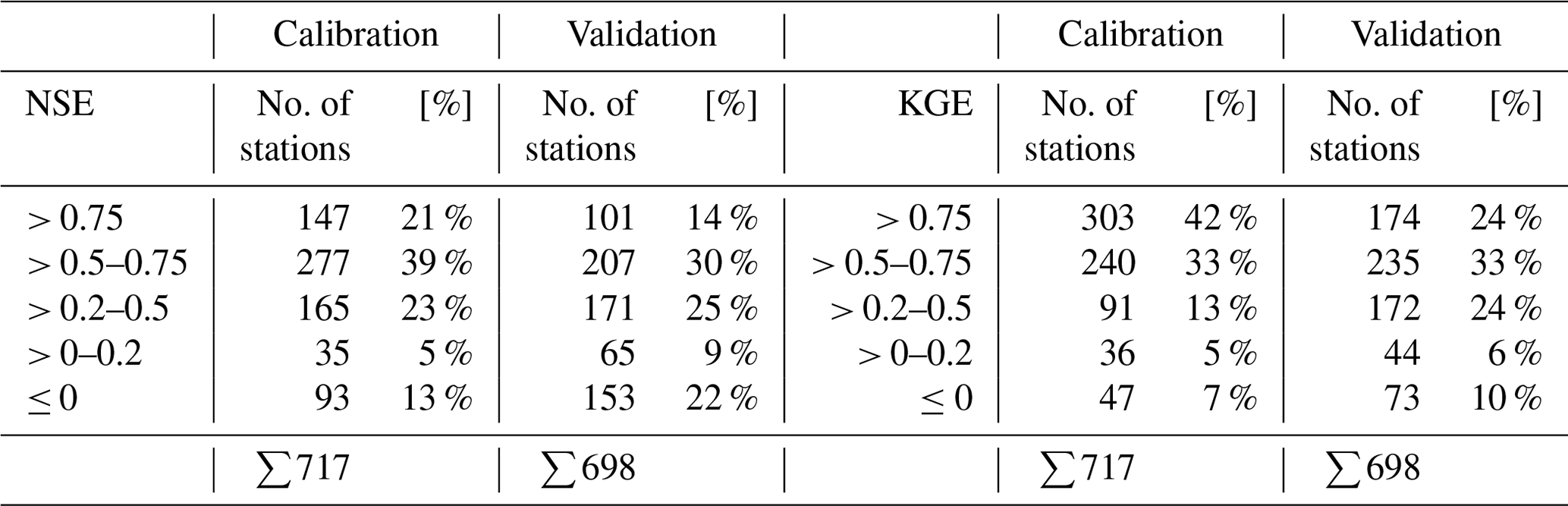
Table B1 summarizes the results of the KGE and NSE indices, and Fig. B1 shows the spatial distribution of the KGE index values across the EFAS domain. The spatial distribution of NSE is roughly similar. For a detailed list of scores for all stations, please refer to Arnal et al. (2019).
As can be seen from Table B1: 75 % of all stations scored a KGE value of higher than 0.5 during calibration, and 57 % did so during validation. NSE index values above 0.5 are scored for 60 % and 44 % of stations for the calibration and validation periods, respectively.
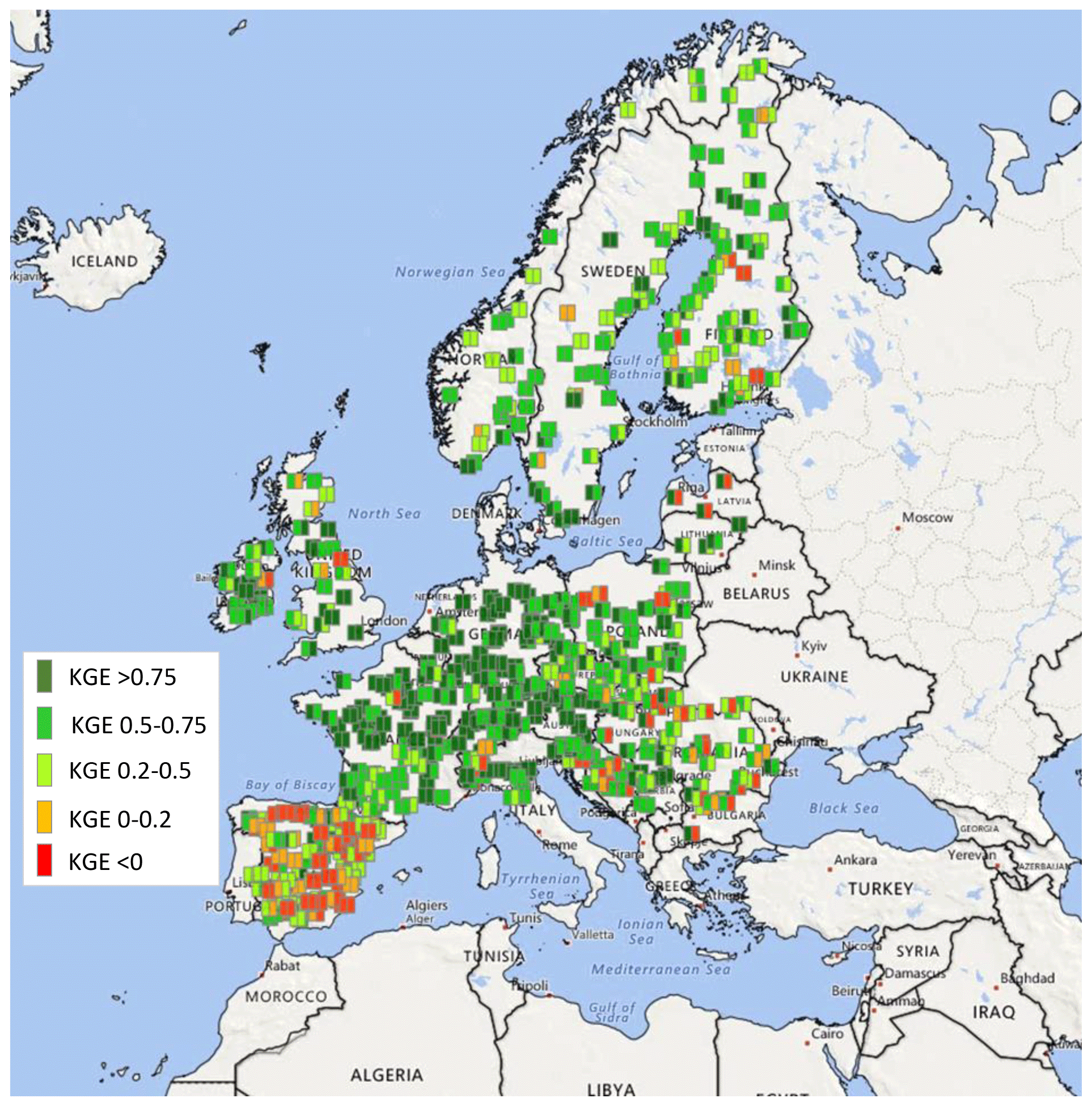
Figure B1Hydrological skill of EFAS at the calibration locations. Colour coding denotes the quality of the KGE during calibration (left half of square) and validation (right half of the square). Adapted from Arnal et al. (2019).

Figure B2Comparison of the empirical and fitted distributions of annual discharge maxima at selected locations of the rivers Rhine (left) and Danube (right).
Table B1Overview of the hydrological skill of LISFLOOD for the calibration and validation stations.
It is clearly noticeable that the skill is not homogeneously distributed across Europe, with higher skills in large parts of central Europe and lower skills mostly in Spain caused by the strong influence of reservoirs and flow control structures. The other study areas considered in the validation exercise (England, Hungary, Norway and Po River basin) exhibit KGE and NSE values generally above 0.5.
B2 Performance of the extreme-value analysis
Here we evaluate the performance of the Gumbel distribution in fitting the available reference discharge values (26 annual maxima calculated for all the grid points of the LISFLOOD long-term run). Specifically, we compare the empirical and fitted distributions of streamflow annual maxima using the Cramér–von Mises test (Anderson, 1962), and we calculate the average differences between reference and fitted discharge values. Table B2 summarizes the resulting p values over the study area. Figure B2 compares empirical and fitted distributions in two locations of the rivers Rhine and Danube.
Table B2Overview of the performance of the Gumbel distribution calculated with the Cramér–von Mises criterion.
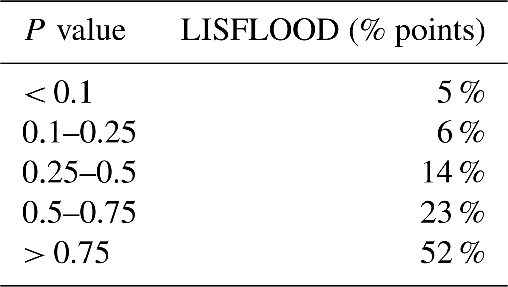
The p values in Table B2 suggest a low skill of the fitted Gumbel distributions; however the resulting uncertainty in the estimates of discharge maxima is generally below 25 %, as in the examples shown in Fig. B2. This is considered acceptable because the reference discharge maxima are modelled and not observed values. Due to the limited sample size, it is not possible to evaluate the extrapolation error for peak flows beyond the available sample; however, previous studies suggested the suitability of the Gumbel distribution. Cunnane (1989) stated that the Gumbel distribution is effective for small sample sizes, whereas the generalized extreme-value (GEV) distribution shows a better overall performance if the size is greater than 50. More recently, Papalexiou and Koutsoyiannis (2013) found similar results for extreme precipitation values. In particular, they demonstrated that short record lengths affects the estimation the GEV shape parameter and thus the choice between a two-parameter (Gumbel) and a three-parameter GEV. Di Baldassarre et al. (2008) observed that the Gumbel distribution might estimate flood extremes with high return periods (e.g. 100 years) with smaller errors than other distributions, if the available sample size is small. Further research could use longer observed streamflow series to compare different extreme-value distributions across European regions, similarly to what was done by Villarini and Smith (2010) for the eastern United States and Rahman et al. (2013) for Australia.
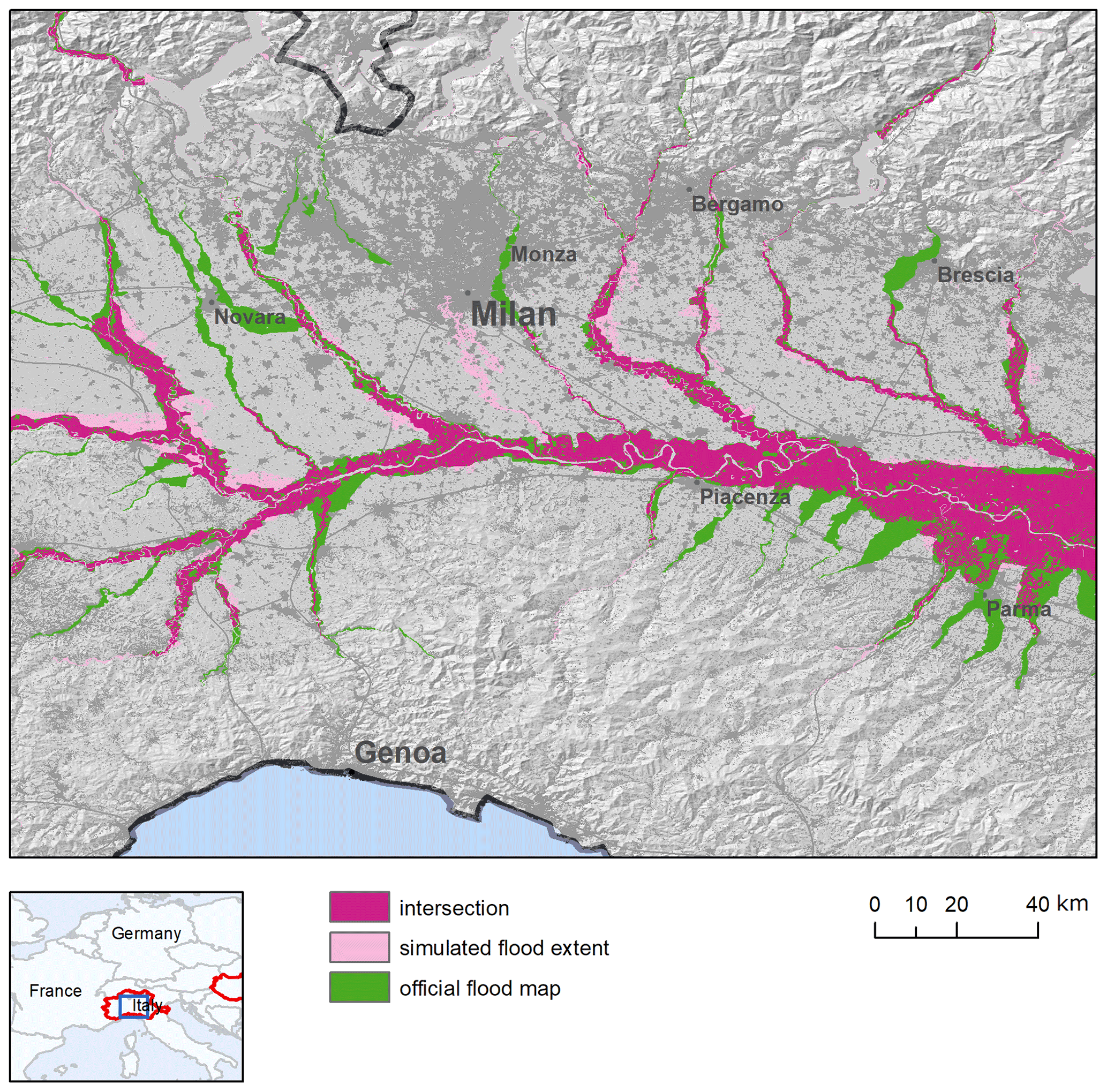
Figure C1Comparison of modelled (blue) and reference (green) flood hazard maps (1-in-500-year flood hazard) over the Po River basin, Italy. Purple areas denote the intersection (agreement) between the two sets of maps.
C1 Validation of the hazard maps for the Po River basin
According to Table 3, the modelled flood maps provide a better reproduction of reference maps for the Po River, compared to other study areas. False alarms are low, while hit rate (HR) values indicate that two out of every three pixels in the reference map are correctly identified as flooded. The analysis of reference and modelled maps (Fig. C1) suggests that the underestimation is partly caused by flooded areas along some tributaries which are not included in modelled maps. Other areas with omission errors are located near confluences of the Po main stem and the major tributaries in Emilia-Romagna, which may depend on the underestimation of peak flow on tributaries. In fact, the results of the LISFLOOD calibration in Fig. B1 show better hydrological skill along the Po main stem, compared to some tributaries. Finally, it is likely that the inclusion of smaller tributaries of the river network in the modelled maps would improve the overall performance.
C2 Validation of the hazard maps for Norway
The results of the modelled flood maps in Norway show a general tendency to overestimate flood extent for the 1-in-100-year events, with high values for both the hit rate (HR) and false-alarm rate (FAR). Such a result is in fact largely influenced by the relatively small extent and discontinuous coverage of reference maps. Flood-prone areas for the 1-in-100-year official maps only cover 215 km2, possibly due to the low density of populated places in Norway, while they cover between 4700 and 5700 km2 for England, Spain and Hungary. As for Spain, we applied a 5 km buffer to restrict the area of comparison around reference maps, yet this leads to spurious overestimation around the edges of reference map polygons. Notably, the performance improves markedly with the use of a 1 km buffer as in Wing et al. (2017), which results in increased critical-success index (CSI) scores up to nearly 0.50.
The results reported by Arnal et al. (2019) and summarized in Fig. B1 suggest an acceptable hydrological skill of the LISFLOOD calibration in Norway, with a majority of gauge stations scoring KGE values above 0.5. In the areas with lower scores, the model performance for low-probability flood events might be influenced by an incorrect estimation of peak discharges driven by snowmelt, which plays a relevant role in determining low-probability flood events.
C3 Influence of correcting elevation data with land use
We tested the results of correcting CCM DEM elevation data with vegetation cover in Scandinavia, where the percentage of land covered by forests is more relevant than in the other regions included in the modelled flood maps. For the 1-in-100-year flood maps, the overall difference in flood extent between the corrected and uncorrected maps is less than 4 %, and similar values were found for the other return periods. Moreover, the HR, FAR and CSI values of two sets of maps differ by less that 2 % when calculated against the 1-in-100-year official map in Norway, probably because forested areas have not been considered relevant flood-prone areas. These results suggest that the simulation of densely vegetated areas have a limited importance in determining the overall performance of modelled flood maps in Europe.
FD conceptualized the project; performed the formal analysis and investigation; curated the data; and wrote, reviewed and edited the paper. LA conceptualized the methodology, performed the investigation, and reviewed and edited the paper. AB curated, validated and visualized the data. JS performed the investigation and reviewed and edited the paper. PS conceptualized and administered the project and wrote, edited and reviewed the paper.
The contact author has declared that neither they nor their co-authors have any competing interests.
Publisher's note: Copernicus Publications remains neutral with regard to jurisdictional claims in published maps and institutional affiliations.
This study has been partially funded by the Copernicus Emergency Management Service and by an administrative arrangement with the Directorate-General for European Civil Protection and Humanitarian Aid Operations (DG ECHO) of the European Commission. EFAS is operated and financed as part of the Copernicus Emergency Management Service. The authors would like to thank Niall McCormick for his valuable suggestions on early versions of the paper.
This research has been supported by the Copernicus Emergency Management Service, which is part of the Copernicus programme, and the EU Civil Protection Mechanism of the European Commission.
This paper was edited by Lukas Gudmundsson and reviewed by Jeffrey Neal and three anonymous referees.
Alfieri, L., Salamon, P., Bianchi, A., Neal, J., Bates, P. D., and Feyen, L.: Advances in pan-European flood hazard mapping, Hydrol. Process., 28, 4928–4937, https://doi.org/10.1002/hyp.9947, 2014.
Alfieri L., Feyen L., Dottori F., and Bianchi A.: Ensemble flood risk assessment in Europe under high end climate scenarios, Global Environ. Chang., 35, 199–212, 2015.
Alfieri, L., Feyen, L., and Di Baldassarre, G.: Increasing flood risk under climate change: a pan-European assessment of the benefits of four adaptation strategies, Climatic Change, 136, 507–521, https://doi.org/10.1007/s10584-016-1641-1, 2016.
Anderson, T. W.: On the Distribution of the Two-Sample Cramer–von Mises Criterion, Ann. Math. Stat., 33, 1148–1159, https://doi.org/10.1214/aoms/1177704477, 1962.
Arnal, L., Asp, S.-S., Baugh, C., de Roo, A., Disperati, J., Dottori, F., Garcia, R., Garcia Padilla, M., Gelati, E., Gomes, G., Kalas, M., Krzeminski, B., Latini, M., Lorini, V., Mazzetti, C., Mikulickova, M., Muraro, D., Prudhomme, C., Rauthe-Schöch, A., Rehfeldt, K., Salamon, P., Schweim, C., Skoien, J. O., Smith, P., Sprokkereef, E., Thiemig, V., Wetterhall, F., and Ziese, M.: EFAS upgrade for the extended model domain – technical documentation, EUR 29323 EN, Publications Office of the European Union, Luxembourg, 2019, JRC111610, ISBN 978-92-79-92881-9, https://doi.org/10.2760/806324, 2019.
Autorita di bacino del fiume Po (AdB Po): Progetto di Variante al PAI: mappe della pericolosita e del rischio di alluvione, https://pianoalluvioni.adbpo.it/progetto-esecutivodelleattivita/ (last access: 3 April 2020), 2012 (in Italian).
Autorità di bacino distrettuale del fiume Po (River Basin District Authority of the Po River): Aree Pericolosità per il Distretto (hazard zones for the District), https://pianoalluvioni.adbpo.it/mappe-del-rischio-2/download-mappe/ last access: 22 March 2022.
Bates, P. D. and De Roo, A. P. J.: A simple raster-based model for flood inundation simulation, J. Hydrol., 236, 54–77, 2000.
Bates, P. D., Horritt, M. S., and Fewtrell, T. J.: A simple inertial formulation of the shallow water equations for efficient two-dimensional flood inundation modelling, J. Hydrol., 387, 33–45, 2010.
Bates, P. D., Quinn, N., Sampson, C., Smith, A., Wing, O., Sosa, J., Savage, J., Olcese, G., Neal, J., Schumann, G., Giustarini, L., Coxon, G., Porter, J. R., Amodeo, M. F., Chu, Z., Lewis-Gruss, S., Freeman, N. B., Houser, T., Delgado, M., Hamidi, A., Bolliger, J., McCusker, K. E., Emanuel, K., Ferreira, C. M., Khalid, A., Haigh, I. D., Couasnon, A., Kopp, R. E., Hsiang, S., and Krajewski, W. F.: Combined modeling of US fluvial, pluvial, and coastal flood hazard under current and future climates, Water Resour. Res., 57, e2020WR028673, https://doi.org/10.1029/2020WR028673, 2021.
Baugh, C. A., Bates, P. D., Schumann G., and Trigg, M. A.: SRTM vegetation removal and hydrodynamic modeling accuracy, Water Resour. Res., 49, 5276–5289, https://doi.org/10.1002/wrcr.20412, 2013.
Barredo, J. I., de Roo, A., and Lavalle, C.: Flood risk mapping at European scale, Water Sci. Technol., 56, 11–17, 2007.
Bontemps, S., Defourny, P., Van Bogaert, E., Arino, O., Kalogirou, V., and Ramos Perez, J.: GLOBCOVER 2009 – Products description and validation report, European Space Agency [data set], http://due.esrin.esa.int/files/GLOBCOVER2009_Validation_Report_2.2.pdf (last access: 17 March 2022), 2011.
Burek, P., van der Knijff, J., and de Roo, A.: LISFLOOD, Distributed Water Balance and Flood Simulation Model Revised User Manual 2013, Publications Office, Luxembourg, 2013.
Copernicus Climate Change Service (Copernicus CCS): River discharge and related historical data from the European Flood Awareness System, https://cds.climate.copernicus.eu/cdsapp#!/dataset/efas-historical, last access: 22 March 2022.
Copernicus Land Monitoring Service (LMS): Corine Land Cover, Copernicus [data set], http://land.copernicus.eu/pan-european/corine-land-cover (last access: 22 March 2022), 2017.
Cunnane, C.: Statistical Distributions For Flood Frequency Analysis, Operational Hydrology Report no. 33, World Meteorological Organization, 1989.
Di Baldassarre, G., Laio, F., and Montanari, A.: Design flood estimation using model selection criteria, Phys. Chem. Earth, 34, 606–611, 2008.
Dottori, F., Salamon, P., Bianchi, A., Alfieri, L., Hirpa, F. A., and Feyen, L.: Development and evaluation of a framework for global flood hazard mapping, Adv. Water Resour., 94, 87–102, 2016a.
Dottori, F., Alfieri, L., Bianchi, A., Lorini, V., Feyen, L., and Salamon, P.: River flood hazard maps for Europe – version 1. European Commission, Joint Research Centre (JRC) [data set], http://data.europa.eu/89h/8e49997c-ba99-4ed1-9aec-059bb440001b (last access: 4 April 2022) 2016b.
Dottori, F., Kalas, M., Salamon, P., Bianchi, A., Alfieri, L., and Feyen, L.: An operational procedure for rapid flood risk assessment in Europe, Nat. Hazards Earth Syst. Sci., 17, 1111–1126, https://doi.org/10.5194/nhess-17-1111-2017, 2017.
Dottori, F., Szewczyk, W., Ciscar, J. C., Zhao, F., Alfieri, L., Hirabayashi, Y., Bianchi, A., Frieler, K., Betts, R. A., and Feyen, L.: Increased human and economic losses from river floods with anthropogenic warming, Nat. Clim. Change, 8, 781–786, https://doi.org/10.1038/s41558-018-0257-z, 2018.
Dottori, F., Bianchi, A., Alfieri, L., Skoien, J., and Salamon, P.: River flood hazard maps for Europe and the Mediterranean Basin region, European Commission, Joint Research Centre (JRC) [data set], https://doi.org/10.2905/1D128B6C-A4EE-4858-9E34-6210707F3C81, 2020a.
Dottori, F., Mentaschi, L., Bianchi, A., Alfieri, L., and Feyen, L.: Adapting to rising river flood risk in the EU under climate change, EUR 29955 EN, Publications Office of the European Union, Luxembourg, 2020, JRC118425, ISBN 978-92-76-12946-2, https://doi.org/10.2760/14505, 2020b.
Environment Agency: Flood Map for Planning (Rivers and Sea) – Flood Zone 3, https://data.gov.uk/dataset/bed63fc1-dd26-4685-b143-2941088923b3/flood-map-for-planning-rivers-and-sea-flood-zone-3, last access: 22 March 2022a.
Environment Agency: Flood Map for Planning (Rivers and Sea) – Flood Zone 2, https://data.gov.uk/dataset/cf494c44-05cd-4060-a029-35937970c9c6/flood-map-for-planning-rivers-and-sea-flood-zone-2, last access: 22 March 2022b.
European Commission (EC): Directive 2007/60/EC of the European Parliament and of the Council on the assessment and management of flood risks, Official Journal of the European Communities, Brussels, http://eur-lex.europa.eu/legal-content/EN/TXT/?uri=CELEX%3A32007L0060 (last access: 13 May 2020), 2007.
European Commission, Joint Research Centre (JRC): Open Source Lisflood, European Commission, Joint Research Centre (JRC) [code]; https://ec-jrc.github.io/lisflood/, last access: 22 March 2022.
ESA-Airbus: Copernicus Digital Elevation Model Validation Report, https://spacedata.copernicus.eu/documents/12833/20611/GEO1988-CopernicusDEM-RP-001_ValidationReport_V1.0/9bc5d392-c5f2-4118-bd60-db9a6ea4a587 (last access: 14 May 2020), 2019.
Feyen, L., Dankers, R., Bódis, K., Salamon, P., and Barredo, J. I.: Fluvial flood risk in Europe in present and future climates, Climatic Change, 112, 47–62, https://doi.org/10.1007/s10584-011-0339-7, 2012.
Fleischmann, A., Paiva, R., and Collischonn, W.: Can regional to continental river hydrodynamic models be locally relevant? A cross-scale comparison, J. Hydrol., 3, 100027, https://doi.org/10.1016/j.hydroa.2019.100027, 2019.
Gupta, H. V., Kling, H., Yilmaz, K. K., and Martinez, G. F.: Decomposition of the mean squared error and NSE performance criteria: implications for improving hydrological modelling, J. Hydrol., 377, 80–91, 2009.
Hirpa, F. A., Salamon, P., Beck, H. E., Lorini, V., Alfieri, L., Zsoter, E., and Dadson, S. J.: Calibration of the Global Flood Awareness System (GloFAS) using daily streamflow data, J. Hydrol., 566, 595–606, 2018.
Jongman, B., Hochrainer-Stigler, S., Feyen, L., Aerts, J. C. J. H., Mechler, R., Botzen, W. J. W., Bouwer, L. M., Pflug, G., Rojas, R., and Ward, P. J.: Increasing stress on disaster-risk finance due to large floods, Nat. Clim. Change, 4, 264–268, https://doi.org/10.1038/nclimate2124, 2014.
Knoben, W. J. M., Freer, J. E., and Woods, R. A.: Technical note: Inherent benchmark or not? Comparing Nash–Sutcliffe and Kling–Gupta efficiency scores, Hydrol. Earth Syst. Sci., 23, 4323–4331, https://doi.org/10.5194/hess-23-4323-2019, 2019.
Krause, P., Boyle, D. P., and Bäse, F.: Comparison of different efficiency criteria for hydrological model assessment, Adv. Geosci., 5, 89–97, https://doi.org/10.5194/adgeo-5-89-2005, 2005.
Kulp, S. A. and Strauss, B. H.: CoastalDEM: A global coastal digital elevation model improved from SRTM using a neural network, Remote Sens. Environ., 206, 231–239, 2018.
Liu, Y., Bates, P. D., Neal, J. C., and Yamazaki, D.: Bare-earth DEM Generation in Urban Areas Based on a Machine Learning Method, in: AGU Fall Meeting Abstracts, Vol. 2019, H41N-1899, 2019.
Maione, U., Mignosa, P., and Tomirotti, M.: Regional estimation of synthetic design hydrographs, Int. J. River Basin Manage., 1, 151–163, 2003.
Meadows, M. and Wilson, M. A.: Comparison of Machine Learning Approaches to Improve Free Topography Data for Flood Modelling, Remote Sens., 13, 275, https://doi.org/10.3390/rs13020275, 2021.
Ministerio de Medio Ambiente y Medio Rural y Marino (MITECO): Guía Metodologica para el desarrollo del sistema nacional de cartografia de zonas inundables, https://www.miteco.gob.es/es/agua/temas/gestion-de-los-riesgos-de-inundacion/snczi/Guia-metodologica-determinacion-zonas-inundables/default.aspx (last access: 18 May 2020), 2011 (in Spanish).
Ministerio para la Transición Ecológica y el Reto Demográfico (Ministry for the Ecological Transition and Demographic Challenge): Zonas Inundables Asociadas a Periodos de Retorno (flood-prone areas related to return periods), https://www.miteco.gob.es/es/cartografia-y-sig/ide/descargas/agua/zi-lamina.aspx last access: 22 March 2022.
Nash, J. E. and Sutcliffe, J. V.: River flow forecasting through conceptual models part I – A discussion of principles, J. Hydrol., 10, 282–290, https://doi.org/10.1016/0022-1694(70)90255-6, 1970.
Noregs Vassdrags- og Energidirektorat (The Norwegian Water Resources and Energy Directorate): Temakart flomsoner – Faresonekart flom (Thematic map flood zones – flood Hazard map), https://www.nve.no/flaum-og-skred/kartlegging/flaum/, last access: 22 March 2022.
Országos Vízügyi Főigazgatóság (National Directorate General for Water Management): Arvízveszély Magyarországon (Danger of Water in Hungary), https://www.vizugy.hu/index.php?module=content&programelemid=62, last access: 22 March 2022.
Papalexiou, S. M. and Koutsoyiannis, D.: Battle of extreme value distributions: A global survey on extreme daily rainfall, Water Resour. Res. 49, 187–201, https://doi.org/10.1029/2012WR012557, 2013.
Paprotny, D., Morales-Nápoles, O., and Jonkman, S. N.: Efficient pan-European river flood hazard modelling through a combination of statistical and physical models, Nat. Hazards Earth Syst. Sci., 17, 1267–1283, https://doi.org/10.5194/nhess-17-1267-2017, 2017.
Rahman, A. S., Rahman, A., Zaman, M. A., Haddad, K., Ahsan, A., Imteaz, M.: A study on selection of probability distributions for at-site flood frequency analysis in Australia, Nat. Hazards 69, 1803–1813, https://doi.org/10.1007/s11069-013-0775-y, 2013.
Sampson, C. C., Smith, A. M., Bates, P. D., Neal, J. C., Alfieri, L., and Freer, J. E.: A high-resolution global flood hazard model, Water Resour. Res., 51, 7358–7381, 2015.
Scussolini, P., Aerts, J. C. J. H., Jongman, B., Bouwer, L. M., Winsemius, H. C., de Moel, H., and Ward, P. J.: FLOPROS: an evolving global database of flood protection standards, Nat. Hazards Earth Syst. Sci., 16, 1049–1061, https://doi.org/10.5194/nhess-16-1049-2016, 2016.
Shaw, J., Kesserwani, G., Neal, J., Bates, P., and Sharifian, M. K.: LISFLOOD-FP 8.0: the new discontinuous Galerkin shallow-water solver for multi-core CPUs and GPUs, Geosci. Model Dev., 14, 3577–3602, https://doi.org/10.5194/gmd-14-3577-2021, 2021.
The Norwegian Water Resources and Energy Directorate (NVE): Flood Zone Maps, https://www.nve.no/flaum-og-skred/kartlegging/flaum/, last access: 24 April 2020 (in Norwegian).
Thielen, J., Bartholmes, J., Ramos, M.-H., and de Roo, A.: The European Flood Alert System – Part 1: Concept and development, Hydrol. Earth Syst. Sci., 13, 125–140, https://doi.org/10.5194/hess-13-125-2009, 2009.
Trigg, M. A., Neal, J. C., Bates, P. D., Smith, A., Sampson, C. C., Yamazaki, D., Hirabayashi, Y. Pappenberger, F., Ward, P. J., Winsemius, H. C., Salamon, P., Dottori, F., Rudari, R., Kappes M. S., and Hadzilacos, G.: The credibility challenge for global fluvial flood risk analysis, Environ. Res. Lett., 11, 094014, https://doi.org/10.1088/1748-9326/11/9/094014, 2016.
United Nations Office for Disaster Risk Reduction (UNISDR): Sendai Framework for Disaster Risk Reduction 2015–2030, http://www.unisdr.org/we/inform/publications/43291 (last access: 25 May 2020), 2015.
University of Bristol: LISFLOOD-FP8.0 with DG2 and GPU solvers, https://www.seamlesswave.com/LISFLOOD8.0, last access: 22 March 2022.
Van der Knijff, J. M., Younis, J., and de Roo, A. P. J.: LISFLOOD: a GIS-based distributed model for river basin scale water balance and flood simulation, Int. J. Geogr. Inf. Sci., 24, 189–212, 2010.
Villarini, G. and Smith, J. A.: Flood peak distributions for the eastern United States, Water Resour. Res., 46, W06504, https://doi.org/10.1029/2009WR008395, 2010.
Vogt, J., Soille, P., De Jager, A., Rimaviciute, E., Mehl, W., Foisneau, S., Bodis, K., Dusart, J., Paracchini, M., Haastrup, P., and Bamps, C.: A pan-European River and Catchment Database, EUR 22920 EN, Luxembourg (Luxembourg), OPOCE, JRC40291, https://doi.org/10.2788/35907, 2007.
Ward, P. J., Jongman, B., Salamon, P., Simpson, A., Bates, P., De Groeve, T., Muis, S., Coughlan de Perez, E., Rudari, R., Trigg, M. A., and Winsemius, H. C.: Usefulness and limitations of global flood risk models, Nat. Clim. Change, 5, 712–715, 2015.
Wendi, D., Liong, S.-Y., Sun, Y., and Doan, C. D.: An innovative approach to improve SRTM DEM using multispectral imagery and artificial neural network. J. Adv. Model. Earth Sy., 8, 691–702, 2016.
Wing, O. E., Bates, P. D., Sampson, C. C., Smith, A. M., Johnson, K. A., and Erickson, T. A.: Validation of a 30 m resolution flood hazard model of the conterminous United States, Water Resour. Res., 53, 7968–7986, https://doi.org/10.1002/2017WR020917, 2017.
Wing, O. E. J., Sampson, C., Bates, P. D., Quinn, N., Smith, A. M., and Neal, J. C.: A flood inundation forecast of Hurricane Harvey using a continental-scale 2D hydrodynamic model, J. Hydrol., 4, 100039, https://doi.org/10.1016/j.hydroa.2019.100039, 2019a.
Wing, O. E. J., Bates, P. D., Neal, J. C., Sampson, C. C., Smith, A. M., Quinn, N., Shustikova, I., Domeneghetti, A., Gilles, D. W., Goska, R., and Krajewskiet W. F.: A New Automated Method for Improved Flood Defense Representation in Large-Scale Hydraulic Models, Water Resour. Res., 55, 11007–11034, https://doi.org/10.1029/2019WR025957, 2019b.
Yamazaki, D., Ikeshima, D., Tawatari, R., Yamaguchi, T., O'Loughlin, F., Neal, J., Sampson, C., Kanae, S., and Bates, P. D.: A high accuracy map of global terrain elevations, Geophys. Res. Lett., 44, 5844–5853, https://doi.org/10.1002/2017GL072874, 2017.
Yamazaki, D., Ikeshima, D., Tawatari, R., Yamaguchi, T., O'Loughlin, F., Neal, J., Sampson, C., Kanae, S., and Bates, P. D.: MERIT DEM: Multi-Error-Removed Improved-Terrain DEM, http://hydro.iis.u-tokyo.ac.jp/~yamadai/MERIT_DEM (last access: 22 March 2022), 2018.
Yamazaki, D., Ikeshima, D., Sosa, J., Bates, P. D., Allen, G. H., and Pavelsky, T. M.: MERIT Hydro: a high-resolution global hydrography map based on latest topography dataset, Water Resour. Res., 55, 5053–5073, https://doi.org/10.1029/2019WR024873, 2019.
Zajac, Z., Zambrano-Bigiarini, M., Salamon, P., Burek, P., Gentile, A., and Bianchi, A.: Calibration of the LISFLOOD hydrological model for Europe, JRC technical report JRC87717, 2013.
- Abstract
- Introduction
- Data and methods
- Results and discussion
- Conclusions and ongoing work
- Data availability
- Appendix A: Meteorological observations used for LISFLOOD simulations
- Appendix B: Calibration and validation of hydrological components
- Appendix C: Additional results
- Author contributions
- Competing interests
- Disclaimer
- Acknowledgements
- Financial support
- Review statement
- References