the Creative Commons Attribution 4.0 License.
the Creative Commons Attribution 4.0 License.
 | 30 Mar 2022
Dataset of daily near-surface air temperature in China from 1979 to 2018
Xueqi Xia
Ping Wang
Jiancheng Shi
Sayed M. Bateni
Tongren Xu
Mengmeng Cao
Essam Heggy
Zhihao Qin
Near-surface air temperature (Ta) is an important physical parameter that reflects climate change. Many methods are used to obtain the daily maximum (Tmax), minimum (Tmin), and average (Tavg) temperature, but are affected by multiple factors. To obtain daily Ta data (Tmax, Tmin, and Tavg) with high spatio-temporal resolution in China, we fully analyzed the advantages and disadvantages of various existing data. Different Ta reconstruction models were constructed for different weather conditions, and the data accuracy was improved by building correction equations for different regions. Finally, a dataset of daily temperature (Tmax, Tmin, and Tavg) in China from 1979 to 2018 was obtained with a spatial resolution of 0.1∘. For Tmax, validation using in situ data shows that the root mean square error (RMSE) ranges from 0.86 to 1.78∘, the mean absolute error (MAE) varies from 0.63 to 1.40∘, and the Pearson coefficient (R2) ranges from 0.96 to 0.99. For Tmin, the RMSE ranges from 0.78 to 2.09∘, the MAE varies from 0.58 to 1.61∘, and the R2 ranges from 0.95 to 0.99. For Tavg, the RMSE ranges from 0.35 to 1.00∘, the MAE varies from 0.27 to 0.68 ∘, and the R2 ranges from 0.99 to 1.00. Furthermore, various evaluation indicators were used to analyze the temporal and spatial variation trends of Ta, and the Tavg increase was more than 0.03 ∘C yr−1, which is consistent with the general global warming trend. In summary, this dataset has high spatial resolution and high accuracy, which compensates for the temperature values (Tmax, Tmin, and Tavg) previously missing at high spatial resolution and provides key parameters for the study of climate change, especially high-temperature drought and low-temperature chilling damage. The dataset is publicly available at https://doi.org/10.5281/zenodo.5502275 (Fang et al., 2021a).
- Article
(12384 KB) - Full-text XML
- BibTeX
- EndNote


Near-surface air temperature (Ta) is an important variable that reflects global climate change and significantly affects the cyclical conversion of energy and matter in all spheres of the earth (Gao et al., 2012, 2014). Obtaining accurate grid Ta is helpful for research on urban heat island effects, ecological environment changes, vegetation phenology development, crop yield fluctuation, and energy dynamic balance (Lin et al., 2012; Bolstad et al., 1998). In this study, Ta refers to the daily maximum (Tmax), minimum (Tmin), and average temperatures (Tavg) of daily near-surface air temperature, which are important input parameters for hydrological, environmental, and crop models (Han et al., 2020; He et al., 2020; Mostovoy et al., 2006; Schaer et al., 2004). These parameters can accurately reflect the frequency and extent of the occurrence and development of extreme climate events (Zhang et al., 2017; Miao et al., 2016). With the intensification of global warming, the temperature gradually rises, the number of extremely cold days and cold nights gradually decreases, and the frequency of extreme weather events also increases (Ding et al., 2006; Liao, 2020; Ryoo et al., 2010). China is a country where extreme weather events frequently occur, causing substantial economic losses (Kharin et al., 2007; Kong, 2020). Therefore, obtaining spatio-temporal changes in Ta is necessary to study extreme weather events and meteorological disasters leading to decreased agricultural yield.
Ta is affected by many factors of the Earth's system, resulting in frequent, complicated diurnal temperature fluctuations (Schwingshackl et al., 2018; Chen et al., 2014). At present, Ta is obtained mainly via three methods: Ta observed via meteorological stations, Ta estimated from land surface temperature (Ts) retrieved from remote sensing, and Ta obtained from the assimilation model. Temperatures with high temporal resolution can be obtained via measurements from meteorological stations. This detection method can avoid the influence of clouds and rain, preserving relatively good data integrity, continuity, and accuracy. However, the number of meteorological stations is limited and they are unevenly distributed, especially for mountainous regions (Mao et al., 2008; Gao et al., 2018; Zhao et al., 2020). Most meteorological stations are in sparsely populated areas far from cities and cannot accurately monitor changes in urban temperature caused by the urban heat island effect (He and Wang, 2020). Moreover, due to the aging of meteorological station equipment, the observation data may be incomplete. Although many interpolation methods, such as Kriging, cubic spline, and inverse distance weight interpolations are available, the difference in density among stations affects the interpolation accuracy (Tang et al., 2020; Berezowski et al., 2016; Tencer et al., 2011).
Satellite sensors provide global coverage and high-spatial-resolution data used to estimate Ta. The most commonly used estimation methods are the statistical regression method (Wen, 2020; Zhu et al., 2013; Zhang et al., 2015), the temperature vegetation index method (Xing et al., 2020), the energy balance method (Benali et al., 2012), the atmospheric temperature profile extrapolation method (Wen, 2020), and the machine learning method (Mao et al., 2008; Wen, 2020). Sensors are susceptible to weather phenomena, such as clouds and rain, leading to missing data or reduced quality. In addition, these methods are mostly suitable for clear-sky conditions, which need to be further expanded to establish an estimation model of Ts to Ta under different weather conditions.
Reanalysis data generated by the global assimilation model have provided many datasets of geophysical parameters, including near-surface temperature, which overcome most of the aforementioned problems caused by abnormal weather. The NCEP/NCAR reanalysis dataset was developed by the National Center for Environmental Prediction and the National Center for Atmospheric Research (January 1948–September 2021), with a temporal resolution of 6 h and a spatial resolution of 2.5∘ (Kalnay et al., 1996). The ERA5 dataset was released by the European Center for Medium-Range Weather Forecast (ECMWF; January 1950–September 2021), with a temporal resolution of 1 h, and a spatial resolution of 0.3∘ (Hersbach et al., 2020; Dee et al., 2011; Taszarek et al., 2021; Lei et al., 2020). The land surface modeling forcing dataset was developed by Princeton University (January 1948–December 2006), with a temporal resolution of 3 h and a spatial resolution of 1.0∘ (Deng et al., 2010). To improve the accuracy of regional data, some researchers have developed meteorological forcing datasets for China. The representative dataset is the China Meteorological Forcing Dataset (CMFD) released by the Institute of Tibetan Plateau Research, Chinese Academy of Sciences (January 1979–December 2018), with a temporal resolution of 3 h and a spatial resolution of 0.1∘ (He, 2010; Yang et al., 2010; Yang and He, 2019). However, the dataset does not provide daily maximum and minimum temperatures. The grid dataset of daily surface temperature in China (V2.0) was released by the China Meteorological Administration (CMA; January 1961–September 2021), with a spatial resolution of 0.5∘. This dataset comprises the daily maximum, minimum, and average temperatures; its spatial resolution is low; and the accuracy of local areas needs improvement. Although reanalysis datasets can obtain global near-surface air temperature data, the number of Tmax, Tmin, and Tavg datasets with high spatial resolution and high precision is insufficient.
In this study, we aimed to obtain a long-term Ta (Tmax, Tmin, and Tavg) dataset with high spatial resolution in China. We first analyzed the advantages and disadvantages of various data (e.g., reanalysis, remote sensing, in situ data). Next, we constructed daily Ta models for clear- and non-clear-sky conditions. This method compensates for the deficiency that studies have estimated Ta mostly under clear-sky conditions rather than under all-sky conditions. We further improve data accuracy by building correction equations for different regions. Finally, a dataset of daily Ta (Tmax, Tmin, and Tavg) in China from 1979 to 2018 was obtained with a spatial resolution of 0.1∘, and we cross-validated this dataset with existing datasets.
China's vast territory has significant undulations on the Earth's surface, and a wide range of climate changes. To explore the temporal and spatial characteristics of Ta, we divided China into six subregions (Fig. 1) according to climatic conditions, such as temperature and rainfall, and topographical conditions, such as elevation. (I) The northeastern region mainly includes Northeast China, located to the east of the Greater Khingan Range. This region is located in the temperate monsoon climate zone, the annual precipitation is 400–1000 mm, and cumulative temperature is between 2500 and 4000 ∘C (Mao and Wan, 2000). (II) The North China region is located north of the Qinling-Huaihe River and south of the Inner Mongolia Plateau. This region is mostly located in the temperate monsoon climate zone, and the annual accumulated temperature is between 3000 and 4500 ∘C (Xu et al., 2017), with hot, rainy summers and cold, dry winters. (III) The central southern region is located south of the Qinling-Huaihe River and north of the tropical monsoon climate type. This region is located in the subtropical monsoon climate zone, the annual accumulated temperature is between 4500 and 8000 ∘C, and the precipitation is mostly between 800 and 1600 mm. (IV) The southern region is south of the Tropic of Cancer. This region is located in the tropical monsoon climate zone, the annual accumulated temperature is greater than 8000 ∘C, the annual minimum temperature is not less than 0 ∘C, and there is no frost year round. Annual precipitation mostly ranges from 1500 to 2000 mm. (V) The northwest region is mainly distributed in the inland areas above 40∘ N latitude in China, located northwest of the Greater Khingan Range-Yin Shan-Ho–lan Mountains-Qilian Mountains line. This region is far from the coast, water vapor transport is limited, annual precipitation is between 300 and 500 mm, and the annual accumulated temperature is between 2000 and 3500 ∘C. The daily and annual temperature differences are large, including those in the temperate desert, temperate grassy, and subfrigid coniferous climates. (VI) The Qinghai-Tibet Plateau region includes the Qinghai-Tibet Plateau, the Andes Mountains, Mount Everest, and other areas. This region is located in the plateau and mountainous climate zone, the annual accumulated temperature is lower than 2000∘, the daily temperature range is large, and the annual temperature range is small. This region has strong solar radiation, sufficient sunshine, and little precipitation.
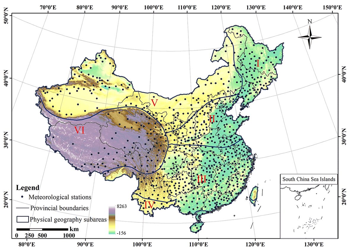
Figure 1Scope map of the total study area and the six subregions. Black dots indicate distribution locations of meteorological stations; blue frame lines indicate the substudy area range, represented by I, II, III, IV, V, and VI.
3.1 Reanalysis data
The reanalysis dataset contains drivers of surface elements in a large area, which can provide highly complementary information and avoid data gaps and low-quality pixels caused by abnormal weather conditions. This study primarily used the CMFD and ERA5 data as reanalysis data sources.
The CMFD is a set of meteorological forcing datasets developed by the Institute of Tibetan Plateau Research, Chinese Academy of Sciences (He et al., 2020; Yang et al., 2010; Yang and He, 2019). It is mainly based on the Global Land Data Assimilation System (GLDAS) as a background dataset, using empirical knowledge algorithms and combining GLDAS with measured data to obtain temperature data with a spatial resolution of 0.1∘. The CMFD contains seven variables: 2 m air temperature, surface pressure, specific humidity, 10 m wind speed, downward shortwave radiation, downward longwave radiation, and precipitation rate. The CMFD covers January 1979 to December 2018 and provides four types of temporal resolution (3 h, daily, monthly, and yearly). The CMFD is comprehensive and has the longest time series and the highest spatial resolution in China. Studies have used the temperature data as input parameters to construct a surface air temperature model, which shows that the correlation coefficient between the CMFD temperature and the measured data is greater than 0.99 and has high consistency, and that grid data can reflect the temporal and spatial changes in regional air temperature (Zhang et al., 2019; Wang et al., 2017). The CMFD as an input element to build a surface temperature model can also significantly reduce model deviation and improve model accuracy (Chen et al., 2011). Therefore, we used the 3 h temperature of the CMFD to build the Ta Model and verified the new product with the daily temperature from the CMFD. The CMFD is available from the China National Qinghai–Tibet Plateau Science Data Center (http://data.tpdc.ac.cn/zh-hans/data/8028b944-daaa-4511-8769-965612652c49/, last access: 1 November 2020).
ERA5 is the fifth-generation product of the atmospheric reanalysis global climate data launched by the ECMWF, replacing the ERA-Interim reanalysis data which were discontinued on 31 August 2019. ERA5 data are generated based on the Cy41r2 model of the integrated forecasting system, which has benefited from the development of data assimilation, model simulation, and model physics, and is generated by assimilating many ground-monitoring, aircraft weather observation, and radio-detection data. ERA5 data are significantly better than ERA-Interim data; for example, the former has a higher spatio-temporal resolution, more vertical mode levels, and more parameter products than the latter. ERA5 provides timely, updated quality checks on the data, which is convenient for providing stable, real-time, and long-term climate information. ERA5 provides many meteorological elements, including 2 m air temperature, 2 m relative humidity, sea level pressure, sea surface temperature, and precipitation. Since the release of the ERA5 reanalysis data, many researchers have tested their applicability and accuracy. The results show that the accuracy of the ERA5 is better than that of the ERA-Interim data, and the higher spatio-temporal resolutions are conducive to the precise description of regional atmospheres. The details of these improvements are convenient for studying changes in small-scale atmospheric environments (Meng et al., 2018; Mo et al., 2021; Hillebrand et al., 2021). These data can be obtained from https://cds.climate.copernicus.eu/cdsapp#!/search?type=dataset&text=ERA5 (last access: 1 December 2020).
3.2 In situ data
The in situ data from 1979 to 2018 used in this study were employed to build a Ta model and evaluate existing datasets and new products. The measured data of meteorological stations were from the China National Meteorological Information Center (http://www.nmic.cn/site/index.html, last access: 1 November 2020), including hourly air temperature, hourly land surface temperature, maximum daily temperature (Tmax), minimum daily temperature (Tmin), daily average temperature (Tavg), and weather condition records. Due to the inconsistency of recorded data of meteorological conditions at many stations, some data are missing. Furthermore, there are no meteorological stations in most areas; thus, the data are used as auxiliary data.
The ground observations obtained from the China Meteorological Administration underwent uniform data processing and homogeneity testing. To further ensure the quality of the data, we checked the in situ data. First, we set a fixed threshold to eliminate the overflow value. Second, we tested the time series of station data and eliminated abnormal and missing data due to instrument damage or bad weather (Zhao et al., 2020). Finally, we checked the spatio-temporal consistency of the in situ data, deleted the meteorological stations with location migration during the study period, and maintained the temperature data of meteorological stations with a long monitoring time and stable temperature values.
3.3 Supplementary data
China's daily near-surface temperature grid dataset was released by the CMA with a spatial resolution of 0.5∘. This grid dataset contains the daily maximum, minimum, and average temperatures in China (http://www.nmic.cn/site/index.html, last access: 11 April 2021). The CMA dataset was obtained by combining the daily temperature data monitored by meteorological stations and the digital elevation model (DEM) data generated by resampling with three-dimensional geospatial information via a thin-plate spline interpolation algorithm. The spatial resolution of the CMA data is 0.5∘, and we used these data for cross-validation. The Moderate Resolution Imaging Spectroradiometer (MODIS) is an important sensor in the Earth Observation System program and is mounted on the Terra and Aqua satellites. Terra is a morning-orbiting satellite that passes through the Equator at approximately 10:30 local time from north to south. Aqua is an afternoon-orbiting satellite that passes through the Equator at approximately 01:30 local time from south to north. The Terra satellite has been in service since 1999, the Aqua satellite since 2002. Since 2002, surface temperature data can be obtained four times per day from MODIS data through inversion calculation. In this study, we used the MOD11A1 and MYD11A1 products, which provide daily surface temperature data on a global scale with a spatial resolution of 1 km. MODIS LST (land surface temperature) has a quality control (QC) field that indicates data quality and is encoded in binary form. MODIS data can be downloaded from the LAADS DAAC (Level-1 and Atmosphere Archive & Distribution System Distributed Active Archive Center) website (https://ladsweb.modaps.eosdis.nasa.gov/search/order, last access: 1 December 2020).
In addition to the aforementioned data, DEM data were used. The Shuttle Radar Topography Mission (SRTM) DEM used in this study was a radar topographic mapping project jointly implemented by NASA and the National Imagery and Mapping Agency, which was implemented by the Space Shuttle Endeavour. Temperature data were regulated via the topographical correction of the SRTM DEM, with 90 m resolution to eliminate the influence of topographical fluctuations on air temperature. SRTM DEM data can be obtained from the Geospatial Data Cloud (http://www.gscloud.cn/search, last access: 10 February 2021).
The Tmax, Tmin, and Tavg data were provided by meteorological stations. Other non-station locations or grid values were estimated by interpolation or indirect methods such as remote sensing. Because of the limited number of meteorological stations and their uneven distribution, it is difficult to guarantee the accuracy of Tmax, Tmin, and Tavg obtained through interpolation in some areas. Under rainfall and cloud-cover weather conditions, estimating the air temperature from remotely sensed surface temperature data is impossible. Even in clear-sky conditions, the formula for estimating near-surface air temperature is not universally applicable, which hinders the development of a high-precision Ta dataset to a certain extent. Therefore, to obtain a Ta dataset with high spatio-temporal resolution and long time series, it is necessary to build a reliable and robust Ta model to estimate Tmax and Tmin, and further improve the accuracy of Tavg. Consequently, the product could be widely used for climate change and research on extreme weather events.
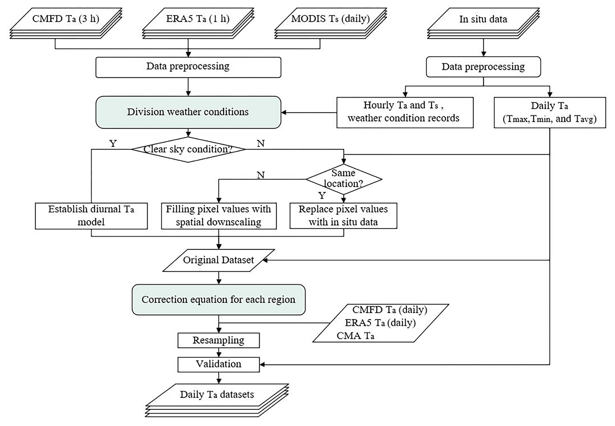
Daily temperature changes are affected by many factors and are extremely sensitive to fluctuations under different weather conditions. This study used multiple methods to calculate Ta. First, the daily weather conditions were divided into clear-sky and non-clear-sky conditions. Second, based on the physical process of daily temperature changes and combined with existing reanalysis data, in situ data, and remote-sensing data, we estimated Tmax and Tmin under different weather conditions. To further improve the accuracy of the dataset, we constructed a modified model for each region. Details are provided in the following sections. The overall process of this study is illustrated in Fig. 2. The construction of the dataset was mainly divided into three steps: (1) the process of daily weather condition determination, (2) the process of establishing Ta models under different weather conditions, and (3) data correction.
4.1 Strategies for division of weather conditions and Ta estimation
4.1.1 Scheme for dividing weather conditions
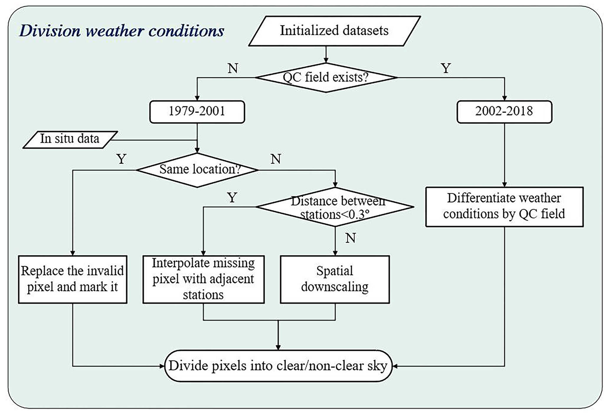
Different weather conditions have different rules of temperature change. To improve the estimation accuracy of the maximum and minimum temperature, we conducted specific calculations by distinguishing daily weather conditions. The quality of observation data is affected by weather, and some remote-sensing products, such as MODIS LST products, have quality control fields. Therefore, the quality control field of MODIS can be used to distinguish between clear-sky and non-clear-sky conditions. However, we have only been able to obtain MODIS observation data four times per day since 2002, which cannot cover the timespan involved in this study. Therefore, we divided the time series of this study into two periods: 1979–2001 and 2002–2018, and different methods were used for the two time series to distinguish the daily weather conditions. For the study period from 2002 to 2018, we distinguished each pixel based mainly on the MODIS quality control field. When the MODIS quality control of all four Ts corresponding to a pixel was in the clear-sky condition, the pixel was judged to be in the clear-sky condition; otherwise, it was judged to be in the non-clear-sky condition.
For the study period from 1979 to 2002, we used the in situ, CMFD, and ERA5 data to determine the daily weather condition. First, we filtered each pixel and divided it into two types: meteorological stations corresponding to pixels with and without weather condition records. For pixels with weather condition records, we used many statistical discrimination methods to analyze the impact of non-clear-sky weather phenomena on temperature fluctuations, which can facilitate the subsequent determination of pixels without weather condition records. Statistical analysis shows a significant difference in daily temperature fluctuations between clear-sky and non-clear-sky conditions, and non-clear-sky weather conditions may cause abnormal temperature fluctuations. Therefore, we converted the judgment of the weather state into the abnormal judgment of the time and frequency of the occurrence of Tmax and Tmin (occurrence time of Tmax and Tmin is hereinafter cited as Hmax and Hmin, respectively). Specifically, when Hmax and Hmin occur abnormally or the temperature change is wavy, a non-clear-sky condition is used (Zhao and Duan, 2014; Ren et al., 2011). In other cases, they are regarded as clear-sky conditions, and the position of each pixel is marked. Therefore, we had to further fill the daily time series of each pixel to determine the weather condition. In this study, we used two strategies to perfect the temperature series for distinguishing weather conditions. The specific implementation steps for determining weather conditions are shown in Fig. 3.
In the first strategy, when the pixel location had a corresponding meteorological station or when the Euclidean distance between adjacent stations was less than 0.3∘, we filled in the gaps to improve the integrity and continuity of the time series. The time series-filling process was as follows: (1) when the temperature data at the observation sites were missing and not consecutively missing, in the case of the same spatial range, we used the average temperature of two adjacent timepoints before and after the missing value at the same site to fill in the missing value; and (2) when the observation data of a station were continuously missing, in the same time range, we filled the missing value with the observation data of the stations within 0.3∘. This method was mainly based on the principle that the closer the distance between stations, the stronger the spatial consistency and correlation of temperature changes. (3) When the station data were continuously missing and the adjacent station data could not be filled, other relevant data were used for repair within the same time and space. In this study, we estimated the weather state from the Ts monitored by the same station. This method theoretically originates from the approximate consistency between the daily variation ranges of Ts and Ta and is suitable for situations where there are many missing values and incomplete time series at meteorological stations and adjacent meteorological stations. Many studies have analyzed the correlation between the daily trend of Ta and Ts and found strong consistency. The Ts retrieved by remote-sensing satellites is also widely used to estimate Ta, which proves the reliability of determining the pixel weather state through the Ts time series (He et al., 2020; Yoo et al., 2018; Johnson and Fitzpatrick, 1977; Caesar et al., 2006; Mostovoy et al., 2006). (4) When there is no meteorological station at the pixel location and the distance from the meteorological station is less than 0.3∘, we use the inverse distance weighting method to perform spatial interpolation on adjacent pixels. Notably, before interpolation, we need to consider the impact of elevation differences. To improve the interpolation accuracy, we first correct the data of the observation station to a uniform sea level, and then perform further calculations according to the elevation of the interpolation point to obtain the corresponding temperature.
The second strategy was to target areas where the distribution of stations was sparse and the Euclidean distance between two adjacent stations was greater than 0.3∘. To compensate for the insufficient coverage and uneven distribution of stations in these areas, we used hourly data from ERA5 to determine the approximate time of occurrence of Tmax and Tmin. Because of a certain difference between the spatial resolution of ERA5 and this dataset, it was difficult to fulfill our demand for higher spatial resolution. Consequently, we developed an effective downscaling process based on the spatial correlation between the ERA5 data and CMFD temperature data. ERA5 data (with a spatial resolution of 0.3∘) were spatially downscaled with the aid of the CMFD data (with a spatial resolution of 0.1∘). The downscaling process is illustrated in Fig. 4. First, quality control of the ERA5 data and CMFD was performed to eliminate temperature outliers. Second, the ERA5 data and CMFD were matched according to time series and central latitude and longitude to construct pixel pairs. Subsequently, we weighted the high-resolution data to the low-resolution ERA5 data pixel by pixel. Finally, the weight was used to downscale the ERA5 data to the same spatial resolution of the CMFD. The ERA5 downscaling was computed using Eqs. (1) and (2),
where TE,TC, and TM represent the ERA5 data, CMFD, and MODIS data, respectively. TE(xo,yo) is the temperature data after downscaling; TE(xm,yn) is the temperature data before downscaling; i, j are pixel coordinates; and m, n are the pixel coordinates before downscaling.

4.1.2 Tmax and Tmin estimation under clear-sky conditions
In addition to the severe temperature fluctuations caused by abnormal weather phenomena, the daily temperature changes under clear-sky conditions have a certain regularity, periodicity, and asymmetry (Leuning et al., 1995; Johnson and Fitzpatrick, 1977). According to the similarity between the surface temperature and the diurnal variation trend of air temperature, a method of estimating Ta is established by the daily air temperature variation model. Verified by in situ data, this method is feasible (Du et al., 2020; Zhu et al., 2013; Perkins et al., 2007; Cesaraccio et al., 2001; Serrano-Notivoli et al., 2019). However, using the surface temperature retrieved by remote-sensing methods to estimate the changing trend of air temperature is complicated, additional parameters need to be input, and the relationship between Ts and Ta is not fixed. Therefore, it is difficult to unify the types and quantities of parameters and ensure accuracy. Thus, we established a piecewise local sine function of temperature under clear-sky conditions for each pixel, which can simulate the change in Ta and calculate Tmax and Tmin (Mao et al., 2016; Jiang et al., 2010). First, according to the approximate periodicity of daily temperature changes and the asymmetry of Hmax and Hmin, we derived the Ta piecewise sine function of the adjacent regions of Hmax and Hmin (Eqs. 3 and 4). Second, using a method similar to that in Sect. 4.1.1, we obtained Hmax and Hmin for each pixel. These Hmax and Hmin values are entered as parameters into the piecewise sine function. The CMFD (3 h data) are used as Ta data, each pixel Hmax and Hmin are used as time, and the values of At and Bt are obtained by the least squares method. Finally, Hmax and Hmin values were substituted into the derivation formula to obtain Tmax and Tmin as preliminary results for subsequent correction and analysis. We constructed a temperature model, pixel by pixel, to fulfill the temporal and spatial heterogeneity of each region.
where Hmax is the occurrence time of the daily maximum temperature, Hmin is the occurrence time of the daily minimum temperature, Ho is the input time, and At and Bt are unknown parameters.
4.1.3 Tmax and Tmin estimation under non-clear-sky conditions
The daily temperature fluctuations in non-clear-sky conditions are relatively large, and there may be large-scale cooling or sudden temperature changes within a short period. Based on the spatial location information of each pixel, the most reliable and representative data source are the in situ data. Therefore, if there are in situ data for the pixel location, the temperature data at the same time will be directly obtained from the station to replace the pixel values Tmax and Tmin. For the pixels corresponding to non-meteorological stations, similar to the method of spatial downscaling for the pixel positions of non-meteorological stations in the weather condition judgment, we used ERA5 data to perform spatial downscaling with the assistance of the CMFD. By adding high-spatial-resolution MODIS data, the downscaling method was further expanded to improve the accuracy of each pixel. We mainly wanted to fully exploit the advantages of various data, especially with the help of high-resolution MODIS data. According to the QC field of MODIS data, we used MODIS data with high spatio-temporal resolution to improve local accuracy while ensuring high-quality MODIS data. The corresponding time of the effective pixel was matched with the ERA5 data according to the nearby time, to obtain the data weight for spatial downscaling. The downscaling process and the validity determination of MODIS data are shown in Fig. 4, and the downscaling formulas are shown in Eqs. (1) and (2).
4.1.4 Tavg estimation
Usually, the aim of calculating average temperature is to use the temperature value observed every day to obtain an arithmetic average. If each pixel has hourly temperature data, the calculated daily average temperature is the most representative. Because the observational conditions are limited, hourly temperature data is difficult to obtain; thus, often, the temperature values of four observation times (e.g., 02:00, 08:00, 14:00, and 20:00) are used to obtain the daily average temperature, or the daily maximum and minimum temperatures are directly averaged to obtain the daily average temperature. To improve the accuracy of the average temperature as much as possible, we used the 3 h temperature data provided by the CMFD and the maximum and minimum values we have calculated to conduct an arithmetic average to obtain the daily average temperature. Finally, to improve the accuracy, we performed multiple linear regression correction on the Tavg output value according to the in situ data (the linear correction method was the same as that described in Sect. 4.2) and obtained the daily Tavg dataset.
4.2 Ta data calibration scheme
Surface temperature is sensitive to changes in altitude and easily affected by the surrounding environment. For non-meteorological station pixels, we use interpolation to fill in the pixel values based on the principle of regional consistency. To improve the accuracy of the pixel temperature at non-meteorological stations, we fully considered the influence of altitude on temperature. First, the in situ Ta was unified to sea level according to the vertical rate of temperature drop. Next, the non-station pixels were interpolated according to the station data, and finally, the interpolated pixel values were restored to the corresponding elevation. This method can reduce the influence of altitude on temperature to a certain extent and improve the accuracy of the dataset. In this study, we used a uniform vertical temperature drop rate (γ), i.e., for every 100 m increase in altitude, the atmospheric temperature decreases vertically by 0.65 ∘C, and vice versa. The height correction formula is provided by Eq. (5) (He and Wang, 2020; Schicker et al., 2015; Wang, 2013):
where TSL is the sea-level temperature, Ta is the temperature of the meteorological station, and HSL is the sea-level height, where the value of γ is approximately 0.0065 ∘C m−1.
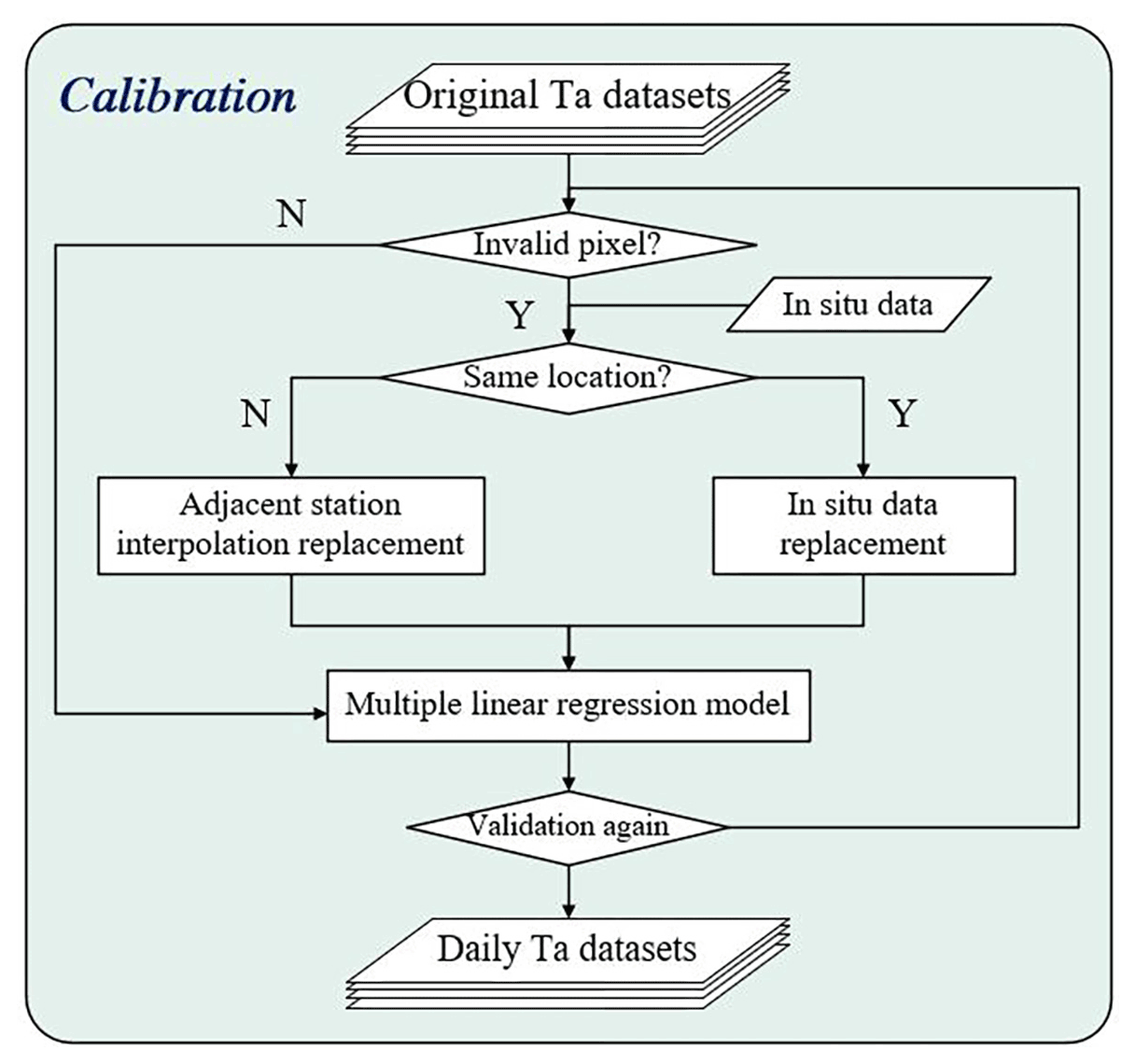
We used the jackknife method as follows: 699 in situ stations across China were divided into 140 verification points and 559 calibration points according to the ratio of 20 to 80 to establish a multiple linear regression equation (Benali et al., 2012; Xu et al., 2017). The preliminary accuracy results (Sect. 5.1) show that although the overall accuracy was high, there remains the problem of abnormal temperature values of the model output data caused by the violent fluctuations in daily temperature changes. Further correction is required to reduce the deviation and improve the accuracy of the dataset. The data correction process is illustrated in Fig. 5. For the abnormal temperature value, we replaced the Ta at the pixel location with the observation Ta from the meteorological station and performed the adjacent pixel temperature correction for the pixel without the meteorological station at the pixel location. The multiple linear regression method was used to process the original temperature, and the stepwise regression relationship between the measured value of the station and the fitted value of the corresponding pixel was established. Next, we calculated the predicted value of the regression temperature according to the regression equation and obtained the temperature residual value by calculating the observed value and the predicted value to obtain the final corrected temperature (Cristobal et al., 2006). The modified expression is shown in Eq. (6):
where x and y are the numbers of rows and columns of pixels, respectively; V(x, y) is the correction value of the regression equation; is the regression prediction value of air temperature; and is the residual value.
4.3 Evaluation metrics
We mainly selected areas with a single surface type and flat terrain under clear skies as the comparative study area to verify the original dataset and reconstructed dataset. A scatter diagram can represent the overall distribution and aggregation of the data and intuitively convey accurate information from the data; thus, we used a scatter chart to display the accuracy range of this product. In addition, before establishing the model, we retained a part of the reanalyzed data excluded from the calculation and used it for cross-validation. We used three indicators as metrics to measure the accuracy of variables, i.e., R2, MAE, and RMSE.
We compared Tmax and Tmin with the ERA5 data and CMA data. Notably, the ERA5 reanalysis dataset is an hourly temperature grid dataset; thus, we obtained the highest and lowest temperature values of ERA5 by constructing a local sine function similar to that in the prior section and further calculated the average daily temperature. The accuracy of Tavg products in this study was verified with the ERA5 data, CMA data, and CMFD daily temperature data. Because the spatial resolution of CMA is 0.5∘, to facilitate comparison, we resampled the spatial resolution of all datasets to 0.5∘.
4.4 Analysis of the Ta series trend
We not only compared the output Ta data with the in situ data, but also assessed the climate change trends of Tmax, Tmin, and Tavg in various regions of China, and further tested the effectiveness and regional applicability of the dataset through various climate variables. The World Meteorological Organization defined a series of extreme climate indexes, including 27 core indexes. We used four of them (TXx, TNn, TX90p, and TN10p) to analyze the trend of extreme temperature changes in Tmax and Tmin (Karl et al., 1999; Peterson et al., 2001). Specifically, the TXx (TNn) anomaly refers to the difference between the sum of monthly Tmax (Tmin) and the multi-year average of monthly Tmax (Tmin) in each year. The multi-year period of this study is 40 years. In addition, linear regression was performed on the TXx (TNn) anomaly to analyze the interannual variation trend. The TX90p (TN10p) means that the daily Tmax (Tmin) of each month during the study period is arranged in ascending order, and the 90 % (10 %) corresponding value in the time series is used as the threshold for judging warm days (cold nights; Zhang et al., 2005).
To study the spatio-temporal variation trend of Tavg, we used linear regression analysis (K), correlation coefficient analysis (R), and the T test (Du et al., 2020; Yan et al., 2020; Cao et al., 2021). The interannual change rate and correlation of Tavg were calculated by K and R, and the formulae are provided by Eqs. (7) and (8), respectively. We performed a two-tailed significance test on the T test to measure the significance of the temperature and time series changes (Eq. 9):
where n represents the total number of years of the time series length, i represents the year, and Ti represents Tavg in the ith year. K>0 indicates that the temperature increases within the time series, and K<0 indicates that the temperature decreases within the time series.
5.1 Evaluation of the original product
According to the six subregions in Fig. 1, comparative analyses of this product (Tmax, Tmin, and Tavg) based on in situ data were conducted. Figure 6 shows the accuracy scatter plot between the original data of Tmax and the in situ data. The R2 fluctuated from 0.91 to 0.99, the MAE ranged from 1.69 to 2.71 ∘C, and the RMSE ranged from 2.15 to 3.20 ∘C. Figure 7 shows the accuracy scatter plot of Tmin. The R2 fluctuated from 0.93 to 0.97, the MAE ranged from 1.34 to 2.17 ∘C, and the RMSE fluctuated from 1.68 to 2.79 ∘C. Figure 8 shows the accuracy scatter plot of Tavg. The R2 fluctuated between 0.97 and 0.99, the MAE ranged from 0.58 to 0.96 ∘C, and the RMSE fluctuated from 0.86 to 1.60 ∘C. As shown in Figs. 6, 7, and 8, the R2 of Tmax, Tmin, and Tavg, and the temperature measured at the meteorological station, were all greater than 0.90. In general, our method performed well in estimating the daily temperature values. However, due to the impact of complex changes in weather, the distribution of temperature values on certain days is discrete, especially in study areas V and VI. Further corrections are necessary to reduce errors and improve the accuracy of the dataset.
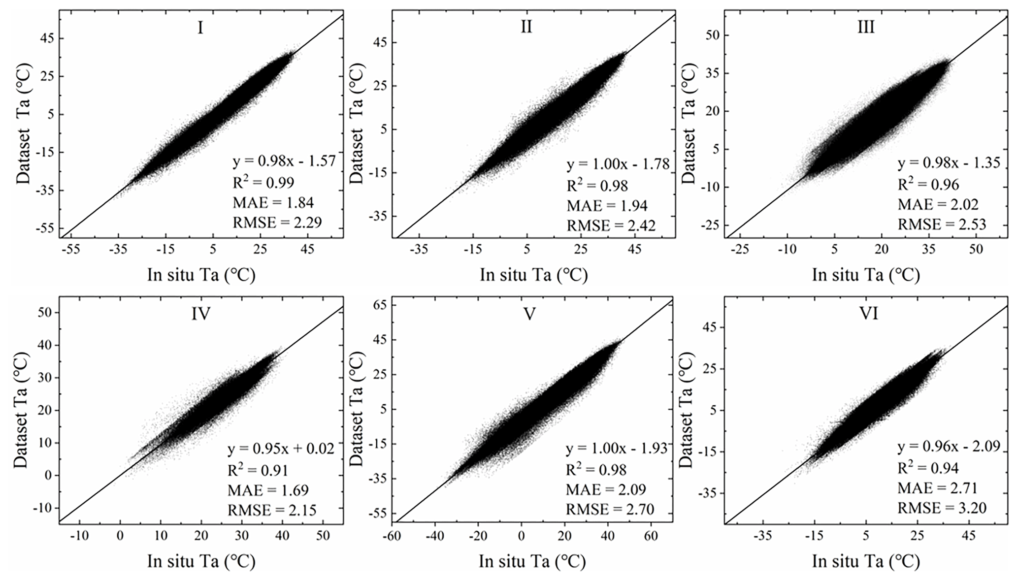
Figure 6Scatter diagrams of the Tmax output from the Ta model against ground station data; statistical accuracy measures (R2, MAE, and RMSE) are also indicated.
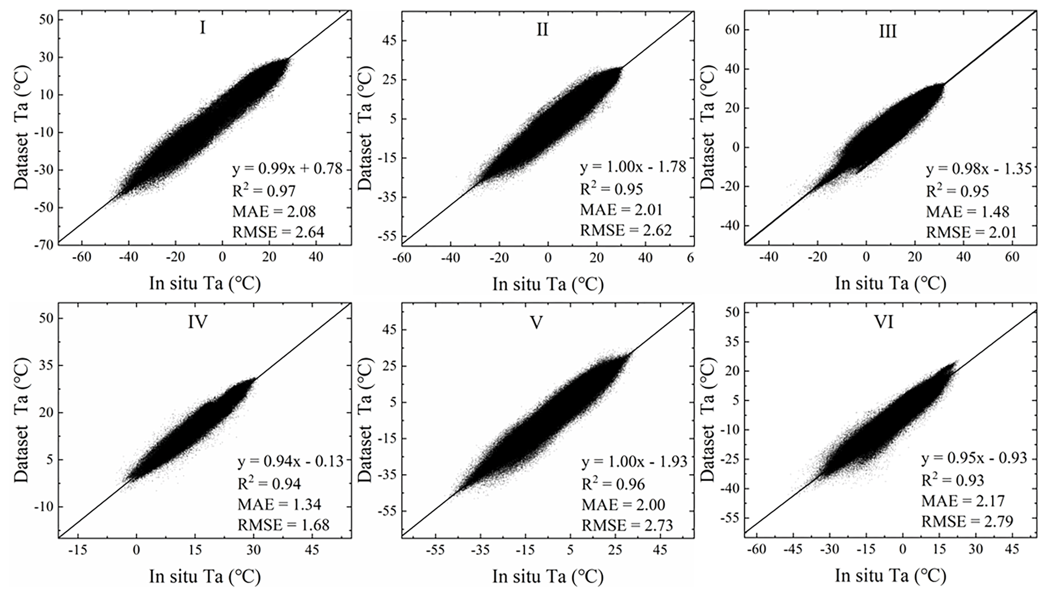
Figure 7Scatter diagrams of the Tmin output from the Ta model against ground station data; statistical accuracy measures (R2, MAE, and RMSE) are also indicated.
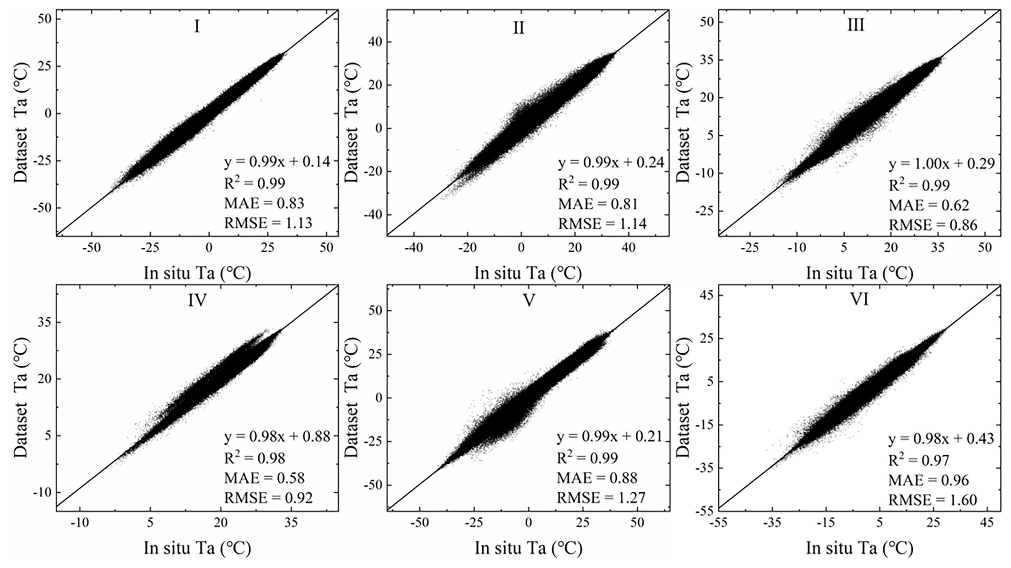
Figure 8Scatter diagrams of the Tavg output from the Ta model against ground station data; statistical accuracy measures (R2, MAE, and RMSE) are also indicated.
5.2 Evaluation of the new product
The temperature was further corrected using the linear correction method. The data verification results of Ta after correction are shown in Figs. 9, 10, and 11. The results show that the corrected data had a higher consistency with the in situ data. The fitted and observed temperatures were linearly distributed and gradually approached the regression line, and the outliers were significantly reduced. Figure 9 shows the corrected scatter plot of Tmax for each study area. The R2 fluctuated from 0.96 to 0.99, the MAE ranged from 0.63 to 1.40 ∘C, and the RMSE fluctuated from 0.86 to 1.78 ∘C. Figure 10 shows the corrected scatter plot of Tmin for each study area. The R2 fluctuated between 0.95 and 0.99, the MAE ranged from 0.58 to 1.61 ∘C, and the RMSE fluctuated from 0.78 to 2.09 ∘C. Figure 11 depicts the corrected scatter plot of Tavg in each study area, where R2 fluctuated between 0.99 and 1.00, the MAE ranged from 0.27 to 0.68 ∘C, and the RMSE fluctuated from 0.35 to 1.00 ∘C. The results show that the distribution of numerical points in each area after the correction was denser, mostly concentrated near the 1:1 line, and the degree of clustering with the measured data was higher than before calibration. Our detailed analysis of the daily temperature in the six study areas demonstrated that the accuracy measurement values differed significantly between the east and west. For example, the accuracy error of study area IV is small, and the accuracy error of study areas VI and V is large, which may be affected by the regional topography and the distribution of meteorological stations. Study area IV is in the tropical monsoon climate zone, affected by latitude and topography, and the temperature is relatively high throughout the year. Moreover, the area is in Eastern China and has densely distributed meteorological stations and relatively flat terrain. Linear correction can significantly improve the agreement between the estimated value and the observed value. Study areas VI and V have the highest RMSE. They are in the Qinghai–Tibet Plateau in Southwest China and Xinjiang in the northwest. Such areas have similar characteristics, such as high altitude, large spatial heterogeneity, and few meteorological stations. This result shows that the temperature has strong spatial heterogeneity. In general, the corrected dataset has higher accuracy than the original dataset, satisfies the spatial heterogeneity of different regions, and better estimates the temperature under different weather conditions.

Figure 9Scatter diagrams of the original Tmax and reconstructed results versus their corresponding ground station data in six natural subregions (I, II, III, IV, V, and VI). Gray points indicate low-quality pixel values in the original Tmax data, orange points represent the values in the after-calibration Tmax dataset; the statistical accuracy measures (R2, MAE, and RMSE) are also indicated.
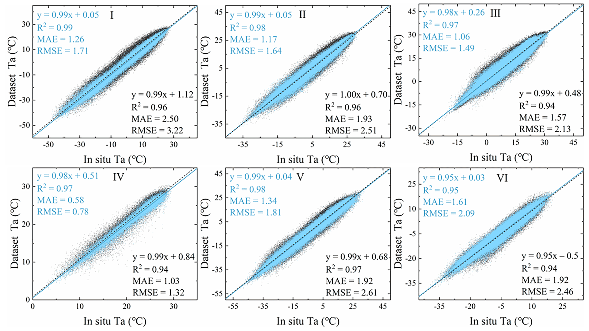
Figure 10Scatter diagrams of the original Tmin and reconstructed results versus their corresponding ground station data in six natural subregions (I, II, III, IV, V, and VI). Gray points indicate low-quality pixel values in the original Tmin data, blue points represent the values in the after-calibration Tmin dataset; the statistical accuracy measures (R2, MAE, and RMSE) are also indicated.
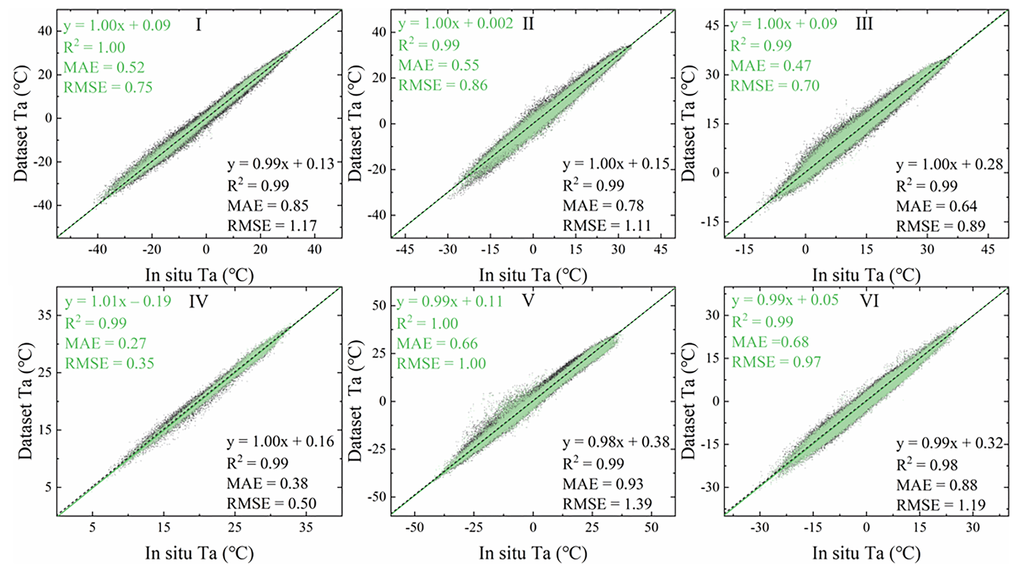
Figure 11Scatter diagrams of the original Tavg and reconstructed results versus their corresponding ground station data in six natural subregions (I, II, III, IV, V, and VI). Gray points indicate low-quality pixel values in the original Tavg data, green points represent the values in the after-calibration Tavg dataset; the statistical accuracy measures (R2, MAE, and RMSE) are also indicated.
To further verify the robustness and accuracy of this product, Table 1 shows the cross-validation results of this product and other datasets, the mean average precision (MAP) of each region, and that this product has a high regional consistency with other datasets. Study area IV in the tropical monsoon climate zone has the highest accuracy, and study area VI located in the Qinghai–Tibet Plateau region of China has the lowest data accuracy. This result may be because the reanalysis dataset is also affected by the number and distribution of meteorological stations and the spatial heterogeneity. The accuracy and robustness of the product were confirmed from another perspective. The accuracy comparison of each area shows that this product has higher accuracy and spatial representation than other datasets. R2 is closer to 1, and MAE and RMSE remain low. Through the accuracy evaluation and data comparison between this product and the existing dataset, we found that our product has a better temperature estimation of each area, and the overall accuracy and accuracy of the dataset are higher.
Table 1 Cross-validation results of this product and other datasets. Values in bold indicate study areas with the highest precision, and values in italics indicate the lowest precision.
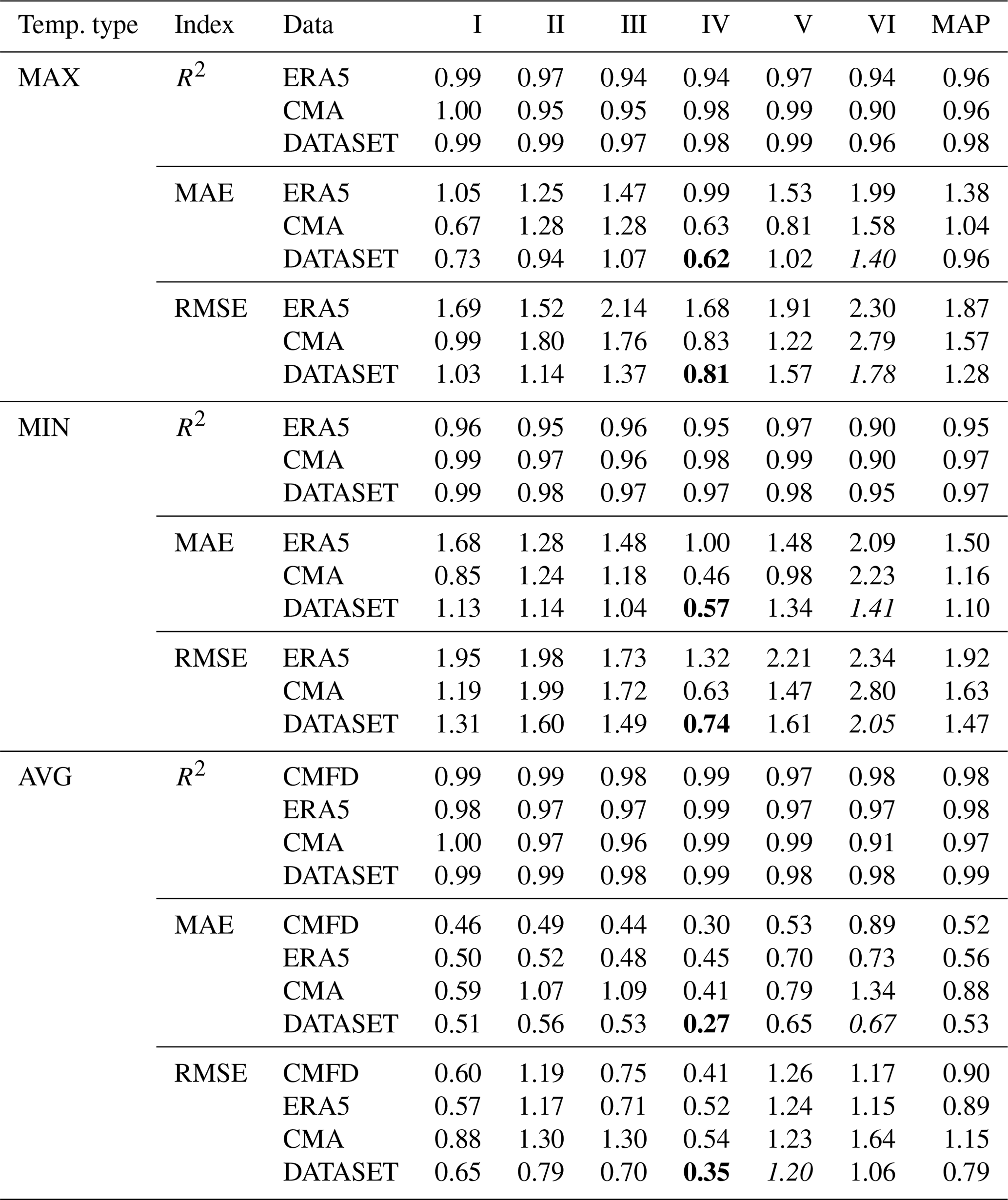
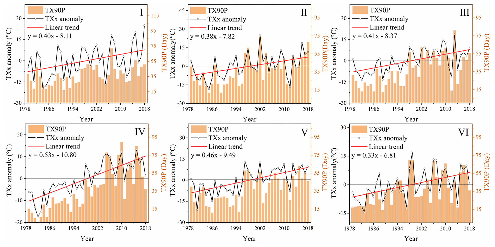
Figure 12Multi-axis diagram of TXx anomaly, TX90p, and Tmax linear trend graphs. The broken black line represents the TXx anomaly, the red line represents the linear regression of the TXx anomaly, and the orange histogram represents the TX90p change trend.
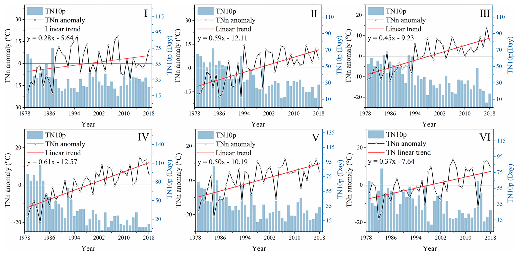
Figure 13Multi-axis diagram of TNn anomaly, TN10p, and Tmin linear trend graphs. The broken black line represents the TNn anomaly, the red line represents the linear regression of the TNn anomaly, and the blue histogram represents the TN10p change trend.
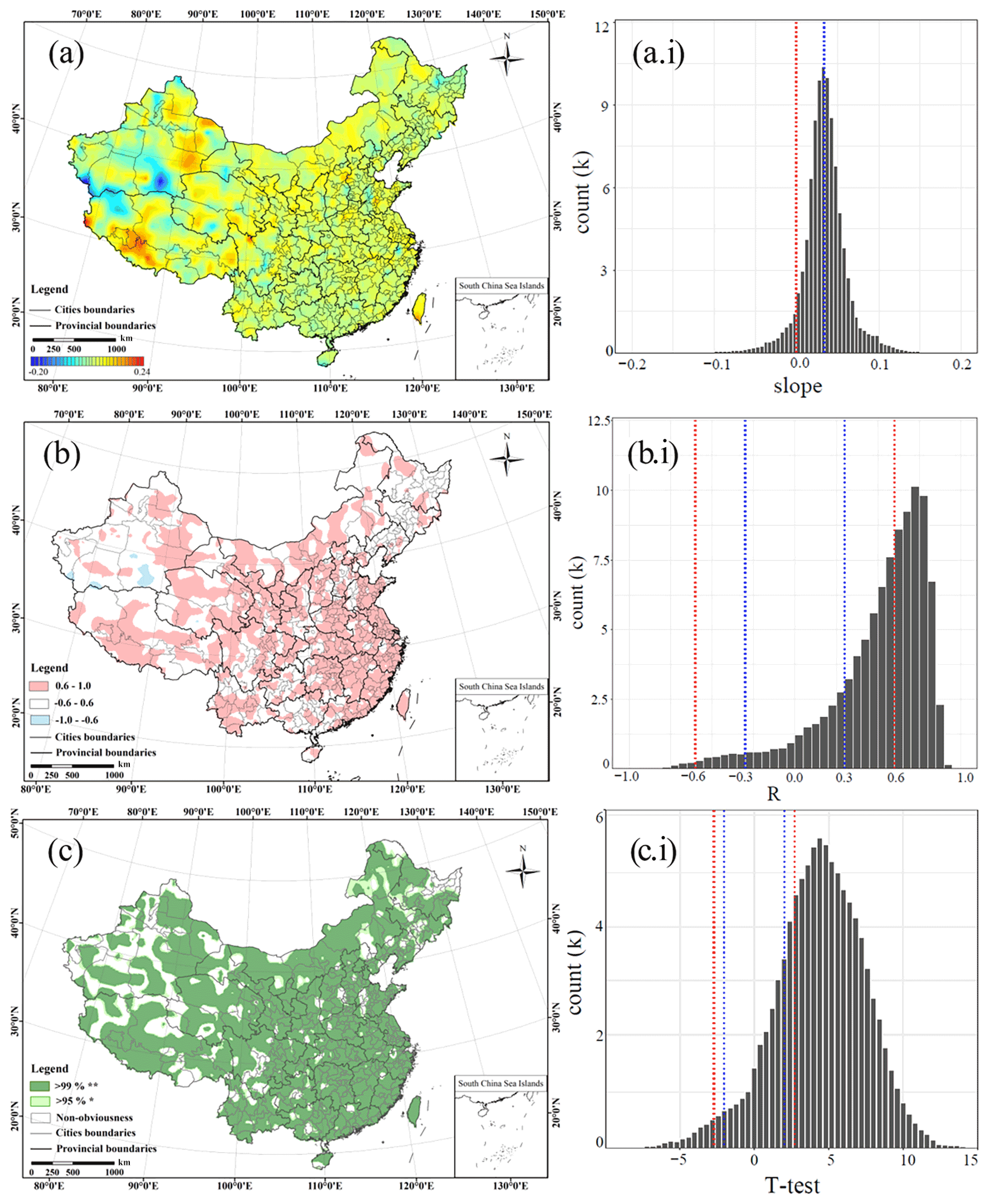
Figure 14Multi-year climate change trends in Tavg. Panel (a) K, as calculated by Eq. (7); (b) R between temperature change and time series development, calculated by Eq. (8); (c) T test (R), calculated by Eq. (9). Panels (a.i), (b.i), and (c.i) represent the distribution of pixel values in the corresponding (a), (b), and (c) spatial images.
5.3 Application of the product for trend analysis
We analyzed temperature changes in various regions of China through extreme climate indexes and change trend values to further test the validity and regional applicability of the dataset. As shown in Figs. 12 and 13, the TXx anomalies and TNn anomalies are consistent in the regional change trend. Although the annual anomalies fluctuated during the study period, they gradually changed from negative to positive. This phenomenon confirmed that the temperature fluctuated and increased, and that the Tmax and Tmin gradually increased, which is consistent with the global warming trend. The average temperature rise of TXx anomalies in each study area was 0.42 ∘C a−1, and the average temperature rise of TXx anomalies was 0.47 ∘C a−1. The histograms in Figs. 12 and 13 show that the number of warm days and cold nights fluctuates in an increasing and decreasing trend, respectively. In addition, similarities are seen in the change trends between warm days and cold nights. For example, in 1980, under the continual influence of strong cold air in the north, low-temperature weather occurred continuously in most areas of China and many areas experienced low-temperature disasters, which led to a decrease in the number of warm days and an increase in the number of cold nights. In 2015, 2016, and 2017, the temperature continued to rise, with high temperatures that occurred once in decades. This finding is closely related to the severe El Niño events that occurred in 2015 and 2016, the impact of the subtropical high in 2017, and the overall global warming trend. From 1979 to 2018, there has also been an increase in the number of warm days and a decrease in the number of cold nights. Meteorological events can indirectly verify the accuracy of this product, indicating that the corrected data can be used to analyze long-term temporal and spatial changes in temperature.
To further analyze the change rate and regional differences in Tavg during the study period, we analyzed the temperature change rate (K), correlation coefficient (R), and significance test of the correlation coefficient (T test(R)). As shown in Fig. 14a and a.i, the Tavg in most regions of China shows a weak positive warming trend, accounting for 92.13 % of the total, and the average temperature of Tavg in each region increased by 0.03 ∘C yr−1. The analysis of R in Fig. 14b and b.i shows that they show a strong correlation of approximately 48.77 % and a correlation in the region of 84.06 %, which shows that there is a high correlation between temperature changes and time. Figure 14c and c.i show that after performing a significance test on the R between temperature and time, 83.17 % of the area passed the 95 % significance test and 75.23 % of the area passed the 99 % significance test, which shows that the correlation between temperature and time development is significant.
The daily Ta products at 0.1∘ resolution from 1979 to 2018 are freely available to the public in tif format at https://doi.org/10.5281/zenodo.5502275 (Fang et al., 2021a), and are distributed under a Creative Commons Attribution 4.0 License.
The technical code of the Ta dataset based on the reconstruction model and verification can be downloaded at https://doi.org/10.5281/zenodo.5513811 (Fang et al., 2021b). We have been finishing and improving the code and plan to upload it as a supplementary version.
Ta is an indispensable variable for global climate change research. Therefore, how to obtain high-precision and high-temporal-resolution air temperature data products is an important issue. Many researchers have endeavored to produce datasets by using different data sources for the global or local region. However, because of the need for refinement of research, further improvements in accuracy and spatio-temporal resolution are necessary. Based on the full analysis of the advantages and disadvantages of various datasets and data sources, this study integrated various data sources, such as in situ data, remote-sensing data, and reanalysis data, and proposes a reconstruction model of Ta under clear-sky and non-clear-sky weather conditions. A multiple linear regression model was used to further improve the accuracy of the data, and we obtained a new set of gridded high-resolution daily temperature datasets in China from 1979 to 2018. For Tmax, validation using in situ data shows that the RMSE ranges from 0.86 to 1.78∘, the MAE varies from 0.63 to 1.40∘, and the R2 ranges from 0.96 to 0.99. For Tmin, the RMSE ranges from 0.78 to 2.09∘, the MAE varies from 0.58 to 1.61∘, and the R2 ranges from 0.95 to 0.99. For Tavg, the RMSE ranges from 0.35 to 1.00∘, the MAE varies from 0.27 to 0.68∘, and the R2 ranges from 0.99 to 1.00. Furthermore, we verified the Ta dataset with the existing reanalysis dataset and found that the proposed dataset has credibility and accuracy. Moreover, based on the particularity of geographic climate change in different regions, we used four extreme climate indicators (TXx and TNn anomalies, TX90p, and TN10p) and three climate change indices (K, R, and T test) to analyze the trend changes of Tmax, Tmin, and Tavg. In summary, the temperature in most regions of China has been gradually increasing. The number of cold nights and warm days has gradually decreased and increased, respectively, and Tmax and Tmin have gradually increased, which is consistent with the general trend of global warming.
However, due to various factors, the weather may occasionally change drastically, such as to hail. Historical data cannot provide weather information to a greater specificity than was possible at that time; thus, particularly in areas without meteorological stations, refining past data is difficult. However, further research should consider more meteorological satellite data, especially geostationary meteorological satellite data, to improve the accuracy of surface temperature datasets used to monitor climate change.
KM designed the research, SF and KM developed the methodology, and wrote the manuscript; XX, PW, JS, SMB, TX, MC, EH, and ZQ revised the manuscript.
The contact author has declared that neither they nor their co-authors have any competing interests.
Publisher’s note: Copernicus Publications remains neutral with regard to jurisdictional claims in published maps and institutional affiliations.
The authors thank the China Meteorological Administration for providing the CMA data and the ground measurements data; the Institute of Tibetan Plateau Research, Chinese Academy of Sciences for the CMFD; and the NASA Earth Observing System Data and Information System for the MODIS LST and DEM data. We also thank the ECMWF for the climate reanalysis data.
This work was supported by the Second Tibetan Plateau Scientific Expedition and Research Program (STEP) “Dynamic monitoring and simulation of water cycle in Asian water tower area” (grant no. 2019QZKK0206), the Framework Project on Application of Space Technology for Disaster Monitoring in the APSCO Member States (global and key regional drought forecasting and monitoring), and the Fundamental Research Funds for Central Nonprofit Scientific Institution (Grant No. 1610132020014).
This paper was edited by Qingxiang Li and reviewed by Minyan Wang and one anonymous referee.
Benali, A., Carvalho, A., Nunes, J., Carvalhais, N., and Santos, A.: Estimating air surface temperature in Portugal using MODIS LST data, Remote Sens. Environ., 124, 108–121, https://doi.org/10.1016/j.rse.2012.04.024, 2012.
Berezowski, T., Szcześniak, M., Kardel, I., Michałowski, R., Okruszko, T., Mezghani, A., and Piniewski, M.: CPLFD-GDPT5: High-resolution gridded daily precipitation and temperature data set for two largest Polish river basins, Earth Syst. Sci. Data, 8, 127–139, https://doi.org/10.5194/essd-8-127-2016, 2016.
Bolstad, P., Swift, L., Collins, F., and Régnière, J.: Measured and predicted air temperatures at basin to regional scales in the southern Appalachian mountains, Agr. Forest Meteorol., 91, 161–176, https://doi.org/10.1016/S0168-1923(98)00076-8, 1998.
Caesar, J., Alexander, L., and Vose, R.: Large-scale changes in observed daily maximum and minimum temperatures: Creation and analysis of a new gridded data set, J. Geophys. Res.-Atmos., 111, 1–10, https://doi.org/10.1029/2005jd006280, 2006.
Cao, M., Mao, K., Yan, Y., Shi, J., Wang, H., Xu, T., Fang, S., and Yuan, Z.: A new global gridded sea surface temperature data product based on multisource data, Earth Syst. Sci. Data, 13, 2111–2134, https://doi.org/10.5194/essd-13-2111-2021, 2021.
Cesaraccio, C., Spano, D., Duce, P., and Snyder, R.: An improved model for determining degree-day values from daily temperature data, Int. J. Biometeorol., 45, 161–169, https://doi.org/10.1007/s004840100104, 2001.
Chen, F., Liu, Y., Liu, Q., and Qin, F.: A statistical method based on remote sensing for the estimation of air temperature in China, Int. J. Climatol., 35, 2131–2143, https://doi.org/10.1002/joc.4113, 2014.
Chen, Y., Yang, K., and He, J.: Improving land surface temperature modeling for dry land of China, J. Geophys. Res.-Atmos., 116, 1–15, https://doi.org/10.1029/2011JD015921, 2011.
Cristobal, J., Ninyerola, M., Pons, X., and Pla, M.: Improving Air Temperature Modelization by Means of Remote Sensing Variables, 2006 IEEE Int. Symp. Geosci. Remote Sensing, 2251–2254, https://doi.org/10.1109/IGARSS.2006.582, 2006.
Dee, D., Uppala, S., Simmons, A., Berrisford, P., Poli, P., Kobayashi, S., Andrae, U., Balmaseda, M., Balsamoa, G., Bauer, P., Bechtold, P., Beljaars, A., Berg, L., Bidlot, J., Bormann, N., Delsol, C., Dragani, R., Fuentes, M., Geer, A., Haimberger, L., Healy, S., Hersbach, H., Hólm, E., Isaksen, L., Kållberg, P., Köhler, M., Matricardi, M., McNally, A., Monge-Sanz, B., Morcrette, J., Park, B., Peubey, C., Rosnay, P., Tavolato, C., Thépaut, J., and Vitart, F.: The ERA-Interim reanalysis: Configuration and performance of the data assimilation system, Q. J. Roy. Meteor. Soc., 137, 553–597, https://doi.org/10.1002/qj.828, 2011.
Deng, X., Zhai, P., and Yuan, C.: Comparison and analysis of several sets of foreign reanalysis data, Meteorol. Sci. Technol., 38, 1–8, https://doi.org/10.19517/j.1671-6345.2010.01.001, 2010.
Ding, Y., Ren, G., Shi, G., Gong, P., Zheng, X., Zhai, P., Zhang, D., Zhao, Z., Wang, S., Wang, H., Luo, Y., Chen, D., Gao, X., and Dai, X.: China's National Assessment Report on Climate Change (I): Climate change in China and the future trend, Clim. Change Res., 2, 3–8, https://doi.org/10.3969/j.issn.1673-1719.2007.z1.001, 2006.
Du, J., Li, K., He, Z., Chen, L., Lin, P., and Zhu, X.: Daily minimum temperature and precipitation control on spring phenology in arid-mountain ecosystems in China, Int. J. Climatol., 40, 2568–2579, https://doi.org/10.1002/joc.6351, 2020.
Fang, S., Mao, K., Xia, X., Wang, P., Shi, J., M. Bateni, S., Xu, T., Cao, M., and Heggy, E.: A dataset of daily near-surface air temperature in China from 1979 to 2018 (Version 1.0), Zenodo [data set], https://doi.org/10.5281/zenodo.5502275, 2021a.
Fang, S., Mao, K., Xia, X., Wang, P., Shi, J., M. Bateni, S., Xu, T., Cao, M., and Heggy, E.: A dataset of daily near-surface air temperature in China from 1979 to 2018 (Version 1.0), Zenodo [code], https://doi.org/10.5281/zenodo.5513811, 2021b.
Gao, L., Bernhardt, M., and Schulz, K.: Elevation correction of ERA-Interim temperature data in complex terrain, Hydrol. Earth Syst. Sci., 16, 4661–4673, https://doi.org/10.5194/hess-16-4661-2012, 2012.
Gao, L., Lu, H., and Chen, W.: Evaluation of ERA-Interim Monthly Temperature Data over the Tibetan Plateau, J. Mt. Sci., 11, 1154–1168, https://doi.org/10.1007/s11629-014-3013-5, 2014.
Gao, L., Wei, J., Wang, L., Bernhardt, M., Schulz, K., and Chen, X.: A high-resolution air temperature data set for the Chinese Tian Shan in 1979–2016, Earth Syst. Sci. Data, 10, 2097–2114, https://doi.org/10.5194/essd-10-2097-2018, 2018.
Han, S., Liu, B., Shi, C., Liu, Y., Qiu, M., and Sun, S.: Evaluation of CLDAS and GLDAS Datasets for Near-Surface Air Temperature over Major Land Areas of China, Sustainability, 12, 1–19, https://doi.org/10.3390/su12104311, 2020.
He, J.: Development of A Surface Meteorological Dataset of China with High Temporal and Spatial Resolution, Institute of Tibetan Plateau Research, CAS, http://ir.itpcas.ac.cn:8080/handle/131C11/1324 (last access: 1 November 2020), 2010.
He, J., Yang, K., Tang, W., Lu, H., Qin, J., Chen, Y., and Li, X.: The first high-resolution meteorological forcing dataset for land process studies over China, Sci. Data, 7, 1–11, https://doi.org/10.1038/s41597-020-0369-y, 2020.
He, Y. and Wang, K.: Contrast patterns and trends of lapse rates calculated from near-surface air and land surface temperatures in China from 1961 to 2014, Sci. Bull., 65, 1217–1224, https://doi.org/10.1016/j.scib.2020.04.001, 2020.
Hersbach, H., Bell, B., Berrisford, P., Hirahara, S., Horányi, A., Muñoz-Sabater, J., Nicolas, J., Peubey, C., Radu, R., Schepers, D., Simmons, A., Soci, C., Abdalla, S., Abellan, X., Balsamo, G., Bechtold, P., Biavati, G., Bidlot, J., Bonavita, M., Chiara, G., Dahlgren, P., Dee, D., Diamantakis, M., Dragani, R., Flemming, J., Forbes, R., Fuentes, M., Geer, A., Haimberger, L., Healy, S., Hogan, R., Hólm, E., Janisková, M., Keeley, S., Laloyaux, P., Lopez, P., Lupu, C., Radnoti, G., Rosnay, P., Rozum, I., Vamborg, F., Villaume, S., and Thépaut, J.: The ERA5 global reanalysis, Q. J. Roy. Meteor. Soc., 10, 1999–2049, https://doi.org/10.1002/qj.3803, 2020.
Hillebrand, F., Bremer, U., Arigony-Neto, J., Rosa, C., Jr, C., Costi, J., Freitas, M., and Schardong, F.: Comparison between Atmospheric Reanalysis Models ERA5 and ERA-Interim at the North Antarctic Peninsula Region, Ann. Am. Assoc. Geogr., 111, 1147–1159, https://doi.org/10.1080/24694452.2020.1807308, 2021.
Jiang, H., Wen, D., Li, N., Ding, Y., and Xiao, J.: A new simulation method for the diurnal variation of temperature-sub-sine simulation, Meteorol. Disaster Reduct. Res., 33, 61–65, https://doi.org/10.3969/j.issn.1007-9033.2010.03.010, 2010.
Johnson, M. and Fitzpatrick, E.: A comparison of two methods of estimating a mean diurnal temperature curve during the daylight hours, Theor. Appl. Climatol., 25, 251–263, https://doi.org/10.1007/BF02243056, 1977.
Kalnay, E., Kanamitsu, M., Kirtler, R., Collins, W., Deaven, D., Gandin, L., Iredell, M., Saha, S., White, G., Woollen, J., Zhu, Y., Chelliah, M., Ebisuzaki, W., Higgins, W., Janowiak, J., Mo, KC., Ropelewski, C., Wang, J., Leetma, A., Reynolds, R., Jenne, R., and Joseph, D.: The NCEP/NCAR 40-year reanalysis project, B. Am. Meteorol. Soc., 77, 437–471, 1996.
Karl, T., Nicholls, N., and Ghazi, A.: CLIVAR/GCOS/WMO workshop on indices and indicators for climate extremes: Workshop summary, Clim. Change, 42, 3–7, https://doi.org/10.1023/A:1005491526870, 1999.
Kharin, V., Zwiers, F., Zhang X., and Hegerl, G.: Changes in Temperature and Precipitation Extremes in the IPCC Ensemble of Global Coupled Model Simulations, J. Climate, 20, 1419–1444, https://doi.org/10.1175/JCLI4066.1, 2007.
Kong, F.: Spatial-temporal differentiation-based evolution characteristics of different extreme air temperature indexes in China from 1961 to 2018, Water Resources and Hydropower Engineering, 51, 67–80, https://doi.org/10.13928/j.cnki.wrahe.2020.04.008, 2020.
Lei, Y., Letu, H., Shang, H., and Shi, J.: Cloud cover over the Tibetan Plateau and eastern China: a comparison of ERA5 and ERA-Interim with satellite observations, Clim. Dynam., 54, 2941–2957, https://doi.org/10.1007/s00382-020-05149-x, 2020.
Leuning, R., Kelliher, F., Depury, D., and Schulze, E.: Leaf nitrogen, photosynthesis, conductance and transpiration-scaling from leaves to canopies, Plant Cell Environ., 18, 1183–1200, https://doi.org/10.1111/j.1365-3040.1995.tb00628.x, 1995.
Liao, Z.: Extreme cold events and interdiural temperature variation at the regional scale in China under global warming background, Chin. Acad. Meteorol. Sci., 3, https://doi.org/10.27631/d.cnki.gzqky.2020.000003, 2020.
Lin, S., Nathan, M., Joseph, M., Mark, D., and Wu, J.: Evaluation of estimating daily maximum and minimum air temperature with MODIS data in east Africa, Int. J. Appl. Earth Obs. Geoinf., 18, 128–140, https://doi.org/10.1016/j.jag.2012.01.004, 2012.
Mao, H. and Wan, H.: Study on the Change of the Accumulated Temperature in North China and Northeast China, Chin. J. Agrometeorol., 3, 2–6, https://doi.org/10.3969/j.issn.1000-6362.2000.03.001, 2000.
Mao, K., Tang, H., Wang, X., Zhou, Q., and Wang, D.: Near-surface air temperature estimation from ASTER data based on neural network algorithm, Int. J. Remote Sens., 20, 6021–6028, https://doi.org/10.1080/01431160802192160, 2008.
Mao, K., Ma, Y., Tan, X., Shen, X., Liu, G., Li, Z., Chen, J., and Xia, L.: Global surface temperature change analysis based on MODIS data in recent twelve years, Adv. Space Res., 59, 503–512, https://doi.org/10.1016/j.asr.2016.11.007, 2016.
Meng, X., Guo, J., and Han, Y.: Preliminarily assessment of ERA5 reanalysis data, J. Mar. Meteorol., 38, 91–99, https://doi.org/10.19513/j.cnki.issn2096-3599.2018.01.011, 2018.
Miao, C., Sun, Q., Duan, Q., and Wang, Y.: Joint analysis of changes in temperature and precipitation on the Loess Plateau during the period 1961–2011, Clim. Dynam., 47, 3221–3234, https://doi.org/10.1007/s00382-016-3022-x, 2016.
Mo, Z., Huang, L., Guo, X., Huang, L., Liu, L., Pang, Z., and Deng, Y.: Accuracy Analysis of GNSS Water Vapor Retrieval in Guilin area using ERA5 data, J. Nanjing Univ. Inf. Sci. Technol. (Nat. Sci. Ed.), 13, 131–137, https://doi.org/10.13878/j.cnki.jnuist.2021.02.001, 2021.
Mostovoy, G., King, R., Reddy, K., Kakani, V., and Filippova, M.: Statistical Estimation of Daily Maximum and Minimum Air Temperatures from MODIS LST Data over the State of Mississippi, GISci. Remote Sens., 43, 78–110, https://doi.org/10.2747/1548-1603.43.1.78, 2006.
Peterson, T., Folland, C., Gruza, G., Hogg, W., Mokssit, A., and Plummer, N.: Report on the Activities of the Working Group on Climate Change Detection and Related Rapporteurs 1998–2001, WMO, 2001.
Perkins, S., Pitman, A., Holbrook, N., and McAneney, J.: Evaluation of the AR4 Climate Models' Simulated Daily Maximum Temperature, Minimum Temperature, and Precipitation over Australia Using Probability Density Functions, J. Climate, 20, 4356–4376, https://doi.org/10.1175/JCLI4253.1, 2007.
Ren, S., Deng, M., and Li, L.: Analysis on the occurrence time of Daily extreme temperature in Kaiping City, Guangdong Meteorol., 33, 35–36, https://doi.org/10.3969/j.issn.1007-6190.2011.04.008, 2011.
Ryoo, S., Kwon, W., and Jhun, J.: Characteristics of wintertime daily and extreme minimum temperature over South Korea, Int. J. Climatol., 24, 145–160, https://doi.org/10.1002/joc.990, 2010.
Schaer, C., Vidale, P., Luethi, D., Frei, C., Haeberli, C., Liniger, M., and Appenzeller, C.: The role of increasing temperature variability in european summer heatwaves, Nature, 427, 332–336, https://doi.org/10.1038/nature02300, 2004.
Schicker, I., Arias, D., and Seibert, P.: Influences of updated land-use datasets on WRF simulations for two Austrian regions, Meteorol. Atmos. Phys., 2015, 128, 279–301, https://doi.org/10.1007/s00703-015-0416-y, 2015.
Schwingshackl, C., Hirschi, M., and Seneviratne, S.: Global Contributions of Incoming Radiation and Land Surface Conditions to Maximum Near-Surface Air Temperature Variability and Trend, Geophys. Res. Lett., 45, 5034–5044, https://doi.org/10.1029/2018GL077794, 2018.
Serrano-Notivoli, R., Beguería, S., and de Luis, M.: STEAD: a high-resolution daily gridded temperature dataset for Spain, Earth Syst. Sci. Data, 11, 1171–1188, https://doi.org/10.5194/essd-11-1171-2019, 2019.
Tang, G., Clark, M. P., Newman, A. J., Wood, A. W., Papalexiou, S. M., Vionnet, V., and Whitfield, P. H.: SCDNA: a serially complete precipitation and temperature dataset for North America from 1979 to 2018, Earth Syst. Sci. Data, 12, 2381–2409, https://doi.org/10.5194/essd-12-2381-2020, 2020.
Taszarek, M., Allen, J., Marchio, M., and Brooks, H.: Global climatology and trends in convective environments from ERA5 and rawinsonde data, NPJ Clim. Atmos. Sci., 4, 1–11, https://doi.org/10.1038/s41612-021-00190-x, 2021.
Tencer, B., Rusticucci, M., Jones, P., and Lister, D.: A Southeastern South American Daily Gridded Dataset of Observed Surface Minimum and Maximum Temperature for 1961–2000, B. Am Meteorol. Soc., 92, 1339–1346, https://doi.org/10.1175/2011BAMS3148.1, 2011.
Wang, C.: Determination of AWS Climate Thresholds by Using Altitude Correction Method, Meteorol. Sci. Technol., 41, 93–96, https://doi.org/10.3969/j.issn.1671-6345.2013.01.018, 2013.
Wang, L., Zhang, X., Fang, Y., and Xia, D.: Applicability Assessment of China Meteorological Forcing Dataset in Upper Yangtze River Basin, Water Power, 43, 18–22, https://doi.org/10.3969/j.issn.0559-9342.2017.03.005, 2017.
Wen, X.: Time series modeling and analysis of remotely sensed land surface temperature over the Tibetan plateau, UESTC, 1, 1–91, https://doi.org/10.27005/d.cnki.gdzku.2020.000994, 2020.
Xing, L., Li, J., and Jiao, W.: Estimation of daily maximum and minimum temperature of Lanzhou City based on MODIS and random forest, Arid Zone Res., 37, 152–158, https://doi.org/10.13866/j.azr.2020.03.17, 2020.
Xu, W., Sun, R., Zhou, S., Jin, Z., and Hu, B.: Estimating daily maximum and minimum air temperatures by remote sensing and GIS, J. B. Norm. Univ (Nat. Sci.), 53, 344–350, https://doi.org/10.16360/j.cnki.jbnuns.2017.03.016, 2017.
Xu, X., Zhang, Y.: China Meteorological background dataset, Resource and Environment Science and Data Center of Chinese Academy of Sciences, https://doi.org/10.12078/2017121301, 2017.
Yan, Y., Mao, K., Shi, J., Piao, S., Shen, X., Dozier, J., Liu, Y., Ren, H., and Bao, Q.: Driving forces of land surface temperature anomalous changes in North America in 2002–2018, Sci. Rep., 10, 1–13, https://doi.org/10.1038/s41598-020-63701-5, 2020.
Yang, K. and He, J.: China meteorological forcing dataset (1979–2018), National Tibetan Plateau Data Center [data set], https://doi.org/10.11888/AtmosphericPhysics.tpe.249369.file, 2019.
Yang, K., He, J., Tang, W., Qin, J., and Cheng, C.: On downward shortwave and longwave radiations over high altitude regions: Observation and modeling in the Tibetan Plateau, Agr. Forest Meteorol., 150, 38–46, https://doi.org/10.1016/j.agrformet.2009.08.004, 2010.
Yoo, C., Im, J., Park, S., and Quackenbushb, L.: Estimation of daily maximum and minimum air temperatures in urban landscapes using MODIS time series satellite data, ISPRS J. Photogramm., 137, 149–162, https://doi.org/10.1016/j.isprsjprs.2018.01.018, 2018.
Zhang, G., Yang, L., Qu, M., and Chen, H.: Interpolation of daily mean temperature by using geographically weighted regression-Kriging, J. Appl. Ecol., 26, 1531–1536, https://doi.org/10.13287/j.1001-9332.20150302.004, 2015.
Zhang, X., Hegerl, G., Zwiers, F., and Kenyon, J.: Avoiding Inhomogeneity in Percentile-Based Indices of Temperature Extremes, J. Climate, 18, 1641–1651, https://doi.org/10.1175/JCLI3366.1, 2005.
Zhang, X., Huang, L., Quan, Q., Zhang, L., Shen, B., and Mo, S.: Relationship of vegetation cover change with climate factors in source region of the Yellow River based on ITPCAS forcing data, J. Northwest A & F Univ. (Nat. Sci. Ed.), 47, 55–68, https://doi.org/10.13207/j.cnki.jnwafu.2019.09.007, 2019.
Zhang, Y., Gao, Z., Pan, Z., Li, D., and Huang, X.: Spatiotemporal variability of extreme temperature frequency and amplitude in China-ScienceDirect, Atmos. Res., 185, 131–141, https://doi.org/10.1016/j.atmosres.2016.10.018, 2017.
Zhao, B., Mao, K., Cai, Y., Shi, J., Li, Z., Qin, Z., Meng, X., Shen, X., and Guo, Z.: A combined Terra and Aqua MODIS land surface temperature and meteorological station data product for China from 2003 to 2017, Earth Syst. Sci. Data, 12, 2555–2577, https://doi.org/10.5194/essd-12-2555-2020, 2020.
Zhao, J. and Duan, Z.: Occurrence of Maximum and Minimum Temperature, Meteorol. Environ. Sci., 37, 86–89, https://doi.org/10.16765/j.cnki.1673-7148.2014.04.012, 2014.
Zhu, W., Lű, A., and Jia, S.: Estimation of daily maximum and minimum air temperature using MODIS land surface temperature products, Remote Sens. Environ., 130, 62–73, https://doi.org/10.1016/j.rse.2012.10.034, 2013.