Beach-face slope dataset for Australia

Sandy beaches are unique environments composed of unconsolidated sediments that are constantly reshaped by the action of waves, tides, currents, and winds. The most seaward region of the dry beach, referred to as the beach face, is the primary interface between land and ocean and is of fundamental importance to coastal processes, including the dissipation and reflection of wave energy at the coast and the exchange of sediment between the land and sea. The slope of the beach face is a critical parameter in coastal geomorphology and coastal engineering, as it is needed to calculate the total elevation and excursion of wave run-up at the shoreline. However, datasets of the beach-face slopes along most of the world's coastlines remain unavailable. This study presents a new dataset of beach-face slopes for the Australian coastline derived from a novel remote sensing technique. The dataset covers 13 200 km of sandy coast and provides an estimate of the beach-face slope every 100 m alongshore accompanied by an easy-to-apply measure of the confidence of each slope estimate. The dataset offers a unique view of large-scale spatial variability in the beach-face slope and addresses the growing need for this information to predict coastal hazards around Australia. The beach-face slope dataset and relevant metadata are available at https://doi.org/10.5281/zenodo.5606216 (Vos et al., 2021).

1 Introduction

The world's coastlines are unique geological environments at the interface between land and sea. Along this coastal fringe, which is often densely populated (Small et al., 2011), we find beaches composed of unconsolidated sediments (e.g. gravel, sand, mud) that are constantly reshaped by the action of waves, currents, winds, and tides (Dean and Dalrymple, 2004). A typical beach cross section, or beach profile, is illustrated in Fig. 1. The beach face is the most seaward region of the subaerial beach, which extends from the berm to the low tide water line and is constantly interacting with the uprush and downrush of individual waves and tidal cycles. The steepness of the beach face (tan β), or the beach-face slope, is a key parameter in coastal geomorphology and coastal engineering due to its control of important coastal processes. Crucially, the beach-face slope controls the elevation of the wave run-up and the total swash excursion at the shoreline (Gomes da Silva et al., 2020; Stockdon et al., 2006), processes that are of primary importance for the assessment of coastal erosion and inundation hazards along the coastal boundary (Senechal et al., 2011; Stockdon et al., 2007). The beach-face slope parameter is also a useful proxy for surf-zone hydrodynamics in the absence of costly surf-zone bathymetric surveys, and can provide insights into beach swimmer safety (Short et al., 1993) and wave set-up across the surf zone (Stephens et al., 2011).

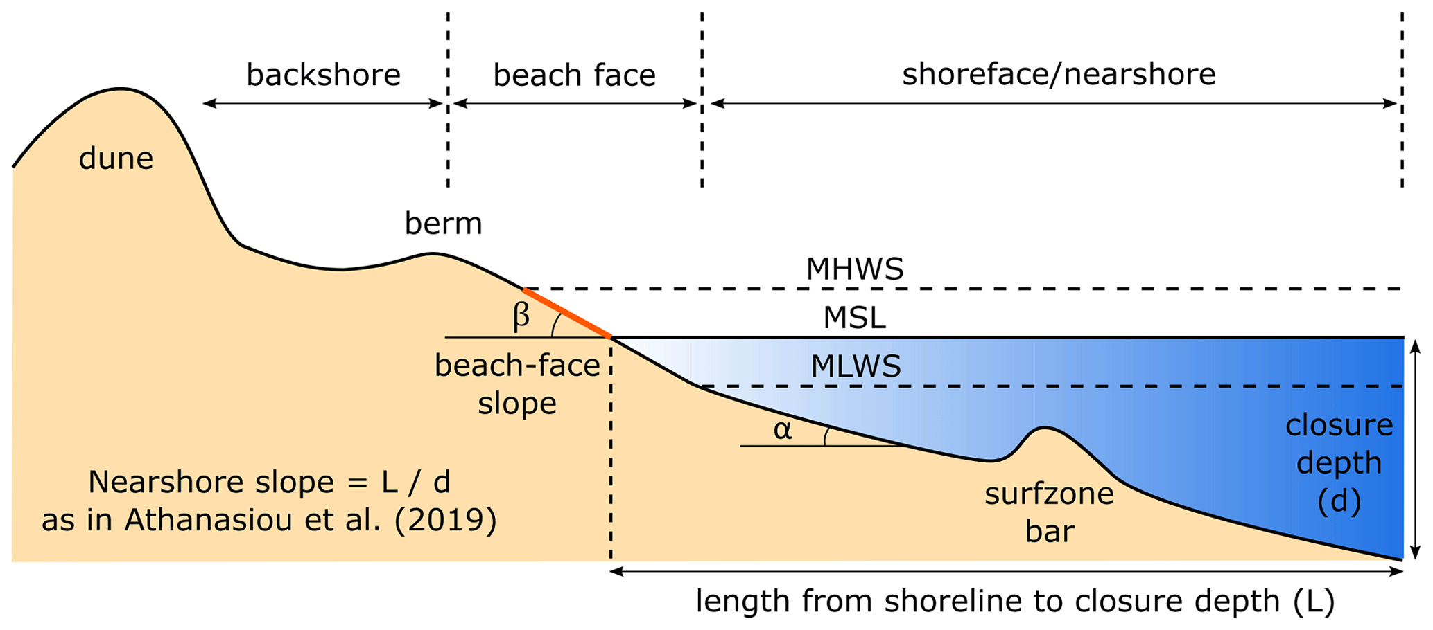
Figure 1 Schematic of a beach profile from the dune to the depth of closure, adapted from Coastal Engineering Research Center (1984). The beach-face slope (tan β) that is mapped in this work is a proxy for the slope of the portion of the profile that is highlighted in orange, extending from mean sea level (MSL) up to mean high water springs (MHWS). The beach-face slope complements the global dataset of nearshore slopes presented in Athanasiou et al. (2019) that represents the slope extending from the depth of closure up to MSL.

Despite the importance of the beach-face slope parameter in numerous empirical formulations in coastal engineering (e.g. wave run-up prediction), large-scale datasets of the beach-face slope remain unavailable along most of the world's coastlines. A complementary global dataset of nearshore slopes, defined from mean sea level (MSL) to the “closure depth” where morphological change is theoretically negligible, was recently compiled by Athanasiou et al. (2019). Referring to Fig. 1, this slope indicates the cross-shore gradient of the subaqueous (below MSL) profile and is generally much lower in gradient than the beach-face slope.

The steepness of the beach face is closely related to grain size (Bujan et al., 2019), with coarser (finer) sediment typically adopting a steeper (flatter) beach face, but it is also linked to the morphodynamic beach state, with lower-gradient slopes usually found along high-energy dissipative beaches and steeper slopes along low-energy reflective beaches (Wright and Short, 1984). The beach-face slope can be measured using survey techniques such as topographic RTK-GPS measurements, but these methods require human intervention and remain impractical over large spatial scales (regional to continental). In recent decades, airborne lidar technology has significantly increased the spatial coverage of coastal topographic data from individual beaches to hundreds of kilometres of coastline (e.g. Middleton et al., 2013; Stockdon et al., 2002). However, in the swash zone, these active remote sensing techniques are hampered by the constant alternation of wet and dry phases as water levels fluctuate at the shoreline under the action of waves and tides (Middleton et al., 2013), limiting the ability to extract beach-face slopes. UAV (unmanned aerial vehicles) surveys and aerial photogrammetry are also subject to the same caveat, as structure-from-motion techniques fail in the swash zone due to the non-stationary ground target (Pucino et al., 2021; Turner et al., 2016). More recently, novel methods to extract intertidal zone information using publicly available optical imagery and tide models have been developed (Bishop-Taylor et al., 2019; Tseng et al., 2017), considerably increasing our ability to map coastal topography over large spatial scales. Recently, Vos et al. (2020) introduced a method to specifically estimate the beach-face slope that combines instantaneous satellite-derived shorelines with predicted tides and is capable of accurately estimating the long-term average slope between the MSL and the mean high water springs (MHWS), the region highlighted in Fig. 1, across a wide range of coastal environments. This new method paves the way for the generation of large-scale beach-face slope datasets to complement the present nearshore slope global dataset and better resolve the coastal topography.

In Australia, a national dataset of coastal topography and bathymetry was recently identified by the marine research, industrial, and stakeholder communities as a key priority to improve the ability to model hazards associated with waves and storm surges (Greenslade et al., 2020). More specifically, O'Grady et al. (2019) investigated the contribution of wind waves to total water levels along the Australian coastline and concluded that a key limitation for an accurate operational coastal inundation forecasting system was the lack of a continental-scale beach-face slope dataset. Historically, due to there being no alternative, studies that have focused on continental to regional scales have adopted uniform beach-face slope values. For example, recent studies investigating the contribution of wave processes to relative sea level rise have either used slope-independent run-up formulations (Vitousek et al., 2017) or opted for a constant and therefore arbitrary beach-face slope of 0.1 for all of the world's coastlines (Melet et al., 2018), which has led to criticism of this approach (Aucan et al., 2019).

In this contribution, we use a recently published and validated beach-face slope estimation technique (Vos et al., 2020) to fill this gap for the Australian continent. We present a new dataset of beach-face slopes spaced at 100 m increments alongshore for every sandy beach in Australia, totalling 13 200 km of sandy coastline. Each beach-face slope estimate is based on the average slope over the past 20 years and is associated with an easy-to-apply measure of confidence. The methodology used to estimate beach-face slopes and confidence bands is presented in the next section. A synopsis then follows of the large-scale spatial variability in beach-face slopes around the Australian continent and the integration of this dataset with the National Sediment Compartment Framework for Australia (Thom et al., 2018). The paper concludes with a brief section illustrating potential use cases of this new dataset for coastal management and flood risk modelling studies.

2 Methods

2.1 Transect dataset

A dataset of shore-normal transects along the Australian sandy coastline was created semi-automatically. Sandy beaches were first extracted from the OpenStreetMaps database (OSM, 2017) and manually quality controlled in a GIS environment (QGIS Development Team, 2021). In total, 5207 sandy beaches were identified along open coasts and semi-enclosed regions. The sandy shoreline locations were then used to generate 100 m alongshore-spaced cross-shore transects with the v_transects functionality of GRASS GIS (GRASS Development Team, 2020), generating a total of 132 000 individual transects extending along 13 200 km of sandy coastline circumnavigating the Australian continent. The beach-face slope was estimated along each transect as described in the following section.

2.2 Beach-face slope estimation algorithm

A novel remote sensing technique to estimate beach-face slopes from satellite imagery and modelled tides was applied to each of the 132 000 sandy beach transects. This method, described in detail in Vos et al. (2020), combines a 20-year time series of shoreline change derived from Landsat imagery with tidal predictions at the time of image acquisition to estimate the slope of the beach face. Briefly, the concept behind this method is that instantaneous shoreline time series mapped onto images acquired at different stages of the tide contain a tidal signal that is modulated by the beach-face slope and can be isolated in the frequency domain due to its periodicity. Thus, this technique uses the frequency domain and iteratively seeks a value of the slope that minimises the tidal energy when used for tidal correction. Tidal correction consists of the projection of individual instantaneous shorelines, acquired at different stages of the tide, to a standard reference elevation such as MSL. A simple tidal correction is then applied by horizontally translating the shoreline points along a cross-shore transect using the linear slope

$$\begin{array}{}\text{(1)}& \mathrm{\Delta }{x}_{\mathrm{corrected}}=\mathrm{\Delta }x+{\displaystyle \frac{z_{\mathrm{tide}}}{\tan \mathit{\beta }}},\end{array}$$

where Δx_corrected is the tidally corrected cross-shore position, Δx is the instantaneous cross-shore position, z_tide is the corresponding tide level, and tan β is the beach-face slope.

The first step is to map instantaneous shorelines spanning a full 20 years of all available Landsat imagery (Landsat 5, 7, and 8) at every sandy beach and then determine the intersection of individual shorelines with each of the 100 m spaced transects to obtain time series of (non-tidally corrected) shoreline change. An example of this is shown in Fig. 2a for Cable Beach, Western Australia. Time series are obtained with CoastSat, a toolbox publicly available at https://github.com/kvos/CoastSat (last access: 7 September 2021​​​​​​) and described in Vos et al. (2019a)​​​​​​​. The 20-year time period (1999–2020) is selected to ensure that two Landsat satellites are in orbit simultaneously, which theoretically results in a combined revisit period of 8 d (16 d for each satellite). However, in practice, time series of shoreline change are irregularly sampled due to factors such as cloud cover, gaps in the Landsat 7 data (scan line corrector error), and discarded images due to poor geometric or radiometric quality. Any outliers in the shoreline time series (e.g. due to false detections) are also removed using a despiking algorithm.

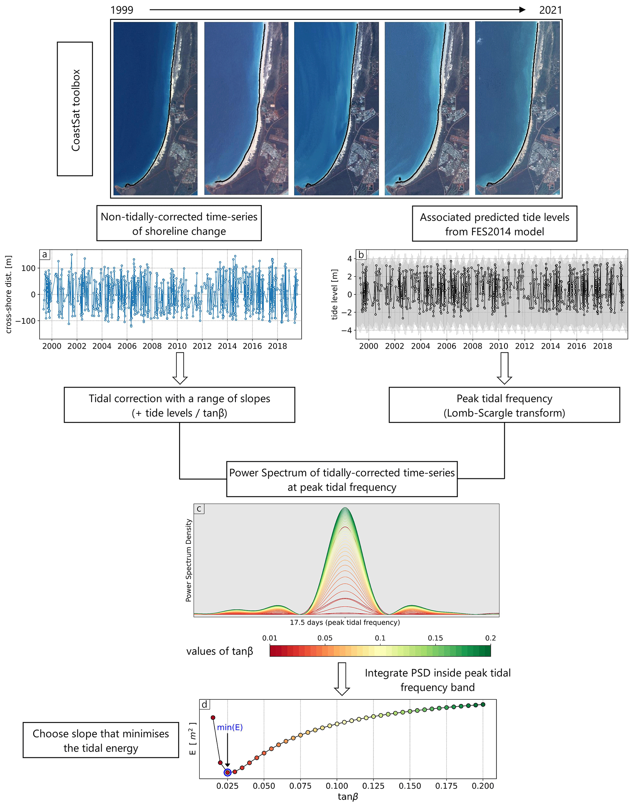
Figure 2 Flowchart of the methodology used to estimate beach-face slopes from satellite-derived shorelines and predicted tides, as described in Vos et al. (2020). Firstly, instantaneous shorelines are mapped onto Landsat imagery with the CoastSat toolbox. The time series of non-tidally corrected shoreline change (a) and their associated tide levels (b) are then combined in the frequency domain to find the slope that, when used for tidal correction, minimises the tidal signal. Panel (c) shows the power spectrum density (PSD) of the tidally corrected time series, demonstrating how the slope value modulates the energy inside the tidal frequency band, which is plotted as a function of slope in (d).

Next, tide levels associated with every shoreline observation are extracted from the global tide model FES2014 (Carrere et al., 2016), as shown in Fig. 2b. The tide-level time series are then transformed to the frequency domain, and since these are not evenly sampled, an alternative to the Fourier transform, the Lomb–Scargle transform (Lomb, 1976; VanderPlas, 2018), is employed to compute the power spectrum density (PSD). Since the Lomb–Scargle is a least-squares spectral method, the limits and spacing of the frequency grid need to be first defined. Here, a main sampling period of 8 days (i.e. the theoretical Landsat revisit period) is used, resulting in a maximum frequency (Nyquist limit) of 16 d, and the spacing n₀ is set to 50 samples per peak to ensure that the grid sufficiently samples each peak (VanderPlas, 2018, Sect. 7.1). In the resulting PSD, the frequency with the highest peak is isolated. This corresponds to the frequency where the tidal signal (e.g. the spring–neap tidal cycle) is strongest in the sub-sampled time series and is referred to as the “peak tidal frequency”. Note that the spring–neap cycle has a period of 14.8 d but is subject to aliasing when sampled at an 8 d interval, resulting in a peak at 17.5 d (refer to Supporting Information S3 in Vos et al., 2020).

The final steps in obtaining the time-averaged estimate of the beach-face slope every 100 m alongshore consists of tidally correcting the time series of raw shoreline change across an iterative range of slope values from 0.01 to 0.2 (following the range identified in Bujan et al., 2019). For each slope value, the tidally corrected time series is transformed to the frequency domain and, by integrating each PSD inside the peak tidal frequency band, a curve of tidal energy vs slope is constructed (Fig. 2c). The best estimate of the beach-face slope is then the value that minimises this tidal energy in the peak tidal frequency band (Fig. 2d). A full example of this procedure is presented for both a microtidal site (Narrabeen-Collaroy) and a macrotidal site (Cable Beach) in the form of Jupyter notebooks at https://github.com/kvos/CoastSat.slope (last access: 2 September 2021, ​​​​​​​Vos, 2021b).

This beach-face slope estimation technique was validated against in situ (beach survey) data along eight diverse sandy/gravel beaches spanning a broad range of beach-face slopes, tidal regimes, and wave climates (Vos et al., 2020). The validation sites – namely Narrabeen-Collaroy, Moruya-Pedro, and Cable Beach in Australia, Duck and Torrey Pines in the USA, Slapton Sands in the UK, Tairua Beach in New Zealand, and Ensenada in Mexico – range from microtidal wave-dominated to macrotidal tide-modified beaches, with the in-situ-measured average beach-face slopes varying from tan β=0.025 to tan β=0.14. The satellite-derived beach-face slope estimates were found to match best with the slope between MSL to MHWS (R²=0.93, bias = 0.0), while they tended to overestimate the full intertidal (MLWS to MHWS) slope. This can be explained by the fact that the upper intertidal slope (MSL to MHWS) is generally more stable over time, while the lower intertidal slope (MLWS to MSL) is more variable as intertidal bars attach to/detach from the shoreline (Wright and Short, 1984). Wave run-up and set-up effects that are not included in the global tide model also tend to skew the shoreline detection towards the upper part of the intertidal profile (e.g. Harley et al., 2019).

2.3 Beach-face slope confidence bands

The tidal energy vs beach-face slope curve shown in Fig. 2d is used to quantify the uncertainty of each beach-face slope estimate. When the minimum is very well defined in the curve (as in Fig. 2d), there is high confidence in the estimate, as there is a single value of the slope that clearly minimises the amount of energy in the peak tidal frequency band. However, at other locations, the minimum of the curve is not so well defined, and several beach-face slope values correspond to similar levels of PSD energy, as shown in Fig. 3 (from Narrabeen-Collaroy beach located in Sydney, NSW). To incorporate a simple-to-apply measure of uncertainty in the dataset of beach-face slope estimates, a 5 % vertical band above the minimum amount of energy in the curve is used to estimate confidence bands around the slope estimate. To illustrate, Fig. 3 shows the 5 % band above the minimum energy, the slope that minimises the energy (0.075), and the lower bound (0.065) and upper bound (0.095) slopes that define the 5 % of the minimum PSD energy. Note that, given the shape of the energy vs beach-face slope curves, which generally tends to start as a parabola and then flattens to an inflection point after the minimum, the confidence bands are not symmetric. While these are not 95 % confidence intervals in the statistical sense, they provide practical information for end users about the uncertainty associated with any individual slope estimate.

Figure 3 Estimation of the confidence band around each beach-face slope estimate based on the tidal energy vs slope curve. The lower and upper bounds are the slopes that are associated with a tidal energy within 5 % of the minimum.

3 Results

3.1 Synopsis of the distribution of beach-face slopes around Australia

Beach-face slopes were estimated at each of the 132 000 beach transects, corresponding to 13 200 km of sandy coastline around Australia. The beach-face slope data were summarised from the transect scale to the individual beach scale by calculating the weighted average of all the transects at each beach; the slopes were weighted by the width of the confidence band to emphasise slopes with higher confidence. The resulting average beach-face slope for every sandy beach around the continent is presented in Fig. 4a. Beach-face slope values range between 0.01 and 0.18. The distribution of beach-face slopes for each of the seven coastal states in Australia is shown in Fig. 4b, which indicates that median values are between 0.055 (Victoria) and 0.08 (Northern Territory), with all seven interquartile ranges sitting between 0.045 and 0.11.

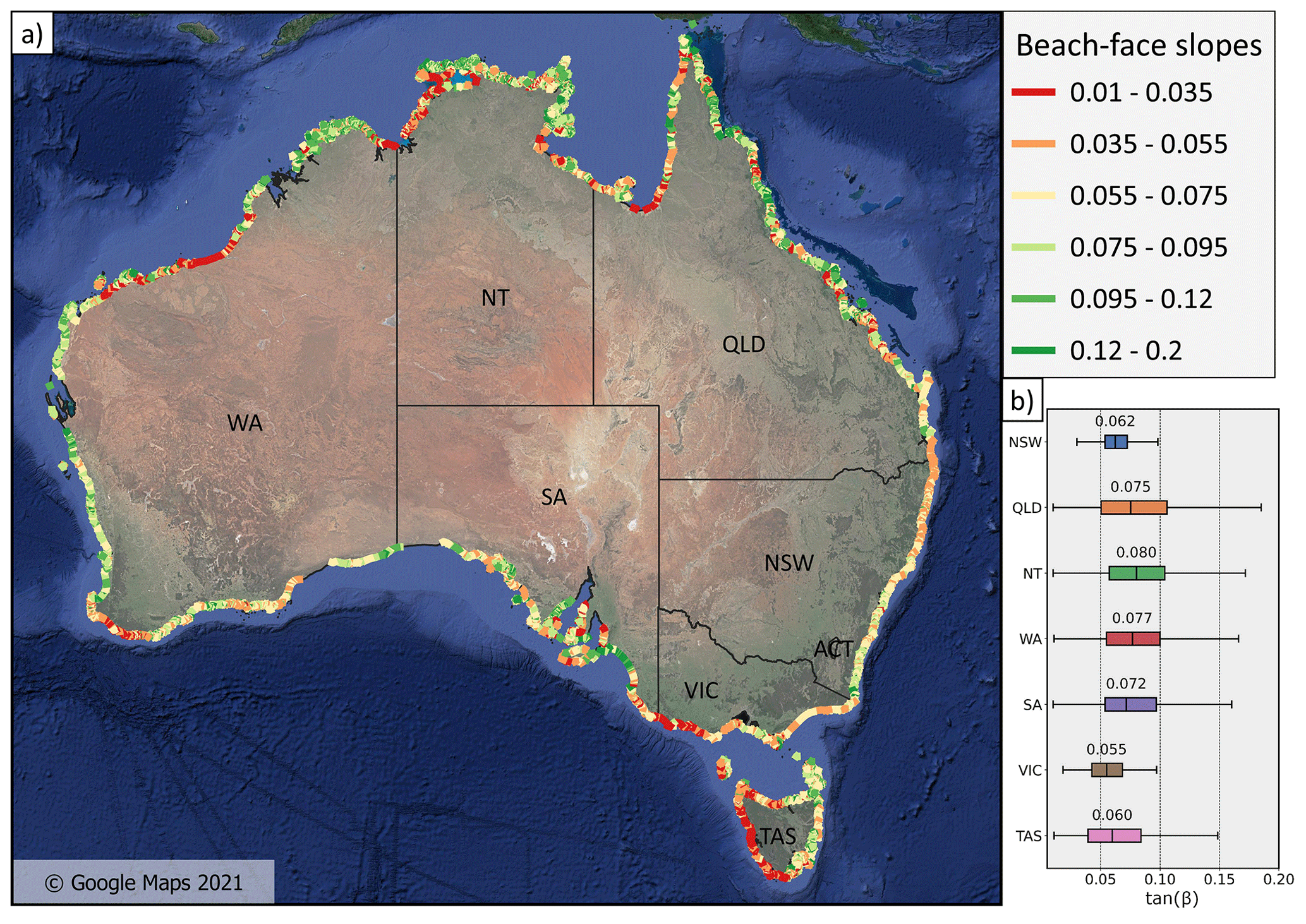
Figure 4 Beach-face slopes around Australia along 132 000 100 m-spaced transects (equivalent to 13 200 km of coast). Panel (b) shows the distribution for each Australian state.

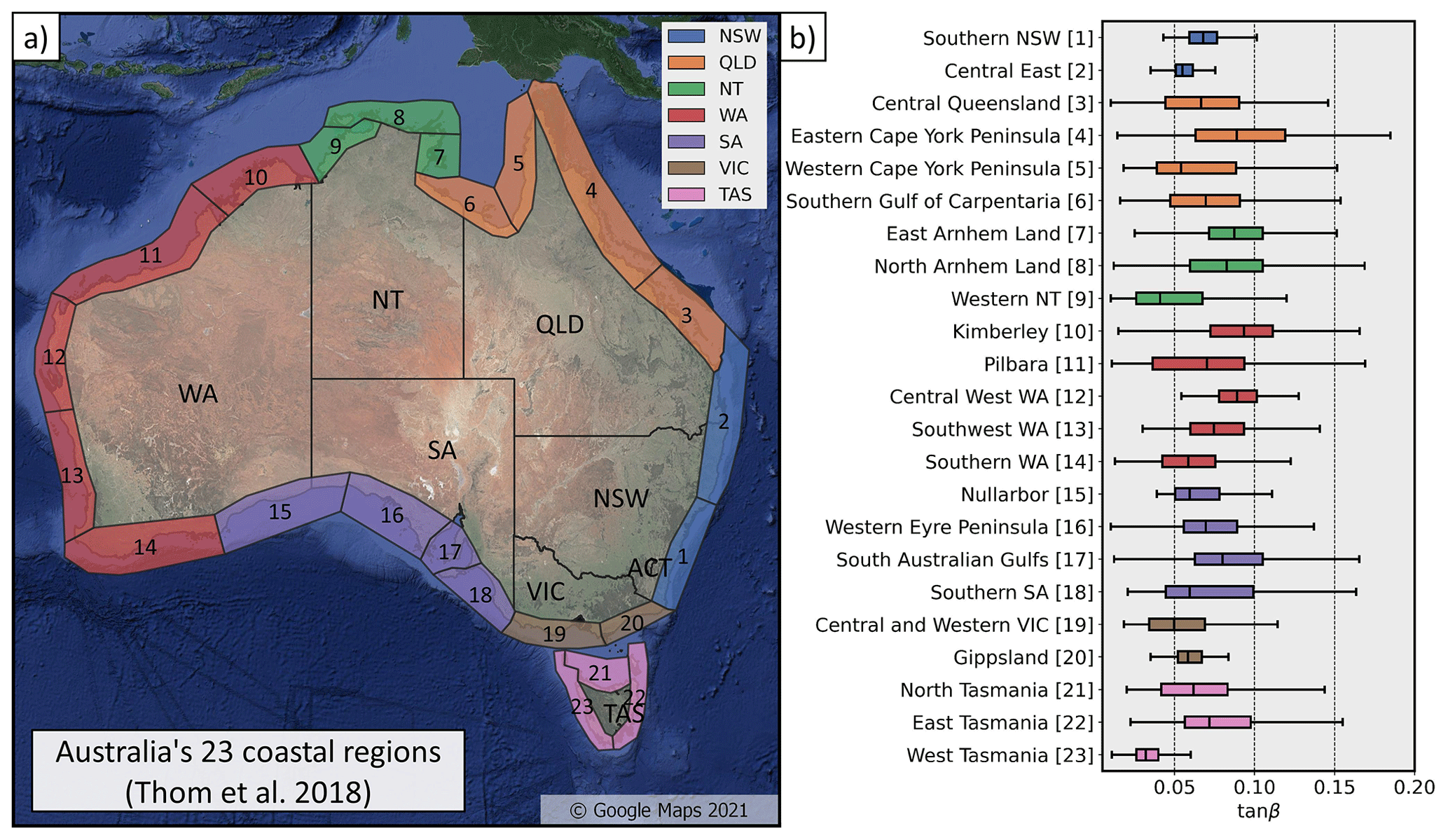
Figure 5 Distribution of beach-face slopes for each of the 23 coastal regions identified by Thom et al. (2018).

Along the wave-dominated and energetic southern half of Australia (refer to Supplement Fig. S1b), the dataset shows very-low-gradient beaches (0.01–0.035) along the western coast of Tasmania, Western Victoria, and Southwest WA. Large spatial variability in the beach-face slopes is observed along the tide-modified/tide-dominated northern half of Australia, with Queensland showing the widest interquartile range (from 0.05 to 0.11).

While state administrative boundaries provide a first division of the country, useful for high-level management purposes, they are not representative of the geology, surface landforms, and shoreline orientation of the Australian coastline. To address this, Thom et al. (2018) proposed a national sediment compartment framework that provides a hierarchical division of the coast, integrating inshore/offshore geological factors, major structural landforms such as headlands, and changes in shoreline orientation. On this basis, the Australian continent is divided into 23 coastal “regions”, 100 “primary sediment compartments”, and 361 “secondary sediment compartments”. The beach-face slope distribution (weighted average per beach) for each of the 23 coastal regions is presented in Fig. 5. Along the south-eastern coast, narrow slope distributions are observed in Central East (2), Southern NSW (1), and Gippsland (20). Moving northwards, very wide distributions are observed in Central Queensland (3), Eastern (4) and Western (5) Cape York Peninsula, and Southern Gulf of Carpentaria (6). The Northern Territory (NT) shows a clear contrast between the relatively steep beaches of East and North Arnhem Land (7–8) and the extremely low-gradient beaches of Western NT (9). A similar distinction is observed in the northern part of Western Australia (WA), where the manifold of islands in the Kimberley region (10) show steep slopes that contrast with the long and low-gradient beaches of the Pilbara region (11). As the tide-modified/tide-dominated coast transitions to a wave-dominated one, a gradient of decreasing beach-face slopes is observed along the western regions of Central West WA (12), Southwest WA (13), and Southern WA (14). Wide beach-face slope distributions are observed in South Australia (SA, regions 15–18), which comprises long microtidal coasts, mesotidal gulfs, and large offshore islands. The remaining region of the continental mainland is Central and Western Victoria (19), which contains relatively low gradient beaches (median of 0.05). Finally, in Tasmania, a clear distinction between the intermediate slopes of the north (21) and east (22) coasts and the west (23) coast is apparent, noting that West Tasmania exhibits the lowest beach-face slopes (median 0.03) of all the coastal regions around Australia.

The widths of the corresponding beach-face slope confidence bands described in Sect. 2.3 provide a simple-to-apply metric and filter on the uncertainty in slope estimates. Figure 6a presents a map of the beach-averaged width of the confidence band. The map is colour coded with a simple three-category “traffic-light” system: high confidence (green) when the confidence-band width is less than 0.025, medium confidence (yellow) when it is between 0.025 and 0.05, and low confidence (red) when it is above 0.05. Using these categories, 56 % of the continental-scale dataset are high-confidence slope estimates, 23 % are medium-confidence estimates, and 21 % are low-confidence estimates. Figure 6b shows the distribution of this confidence metric across each of the 23 regions. Extensive areas of low-confidence estimates are observed along the west and south coasts of WA and most of SA, while the remainder of the coastline generally presents high-confidence estimates interspersed with isolated occurrences of low/medium-confidence estimates (e.g. East Arnhem Land, southern part of East Tasmania). The median width of confidence bands is below 0.025 (i.e. high confidence) for 13 of the 23 coastal regions, between 0.025 and 0.5 (medium confidence) for five regions (East Arnhem Land, Central West WA, Western Eyre Peninsula, East/West Tasmania), and above 0.5 (low confidence) for five regions (including Southwest and Southern WA and the majority of SA).

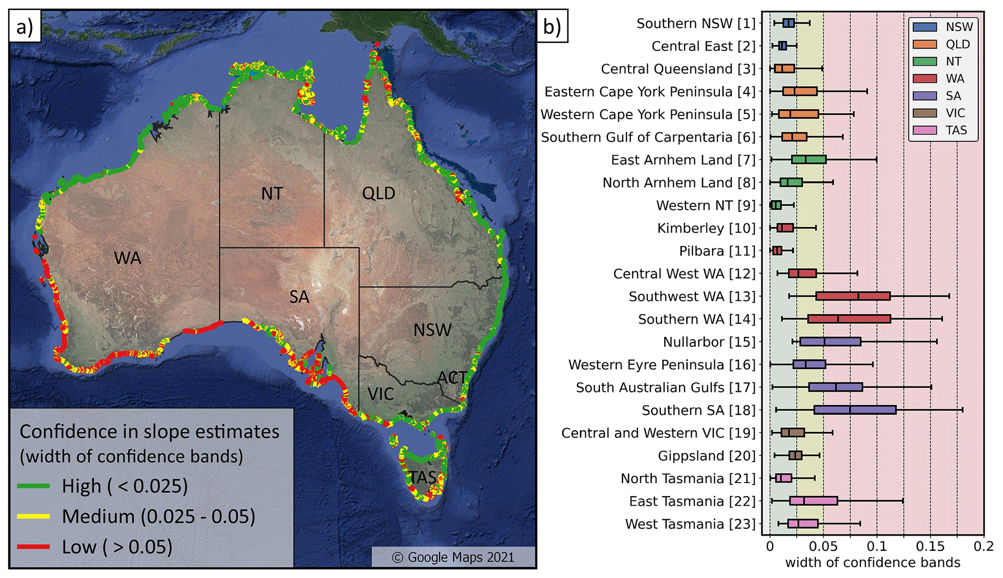
Figure 6 Traffic-light system indicating the uncertainty in the beach-face slope estimates. Panel (b) shows the distribution of the widths of confidence bands across the 23 regions, indicating on average high confidence across 13 regions, medium confidence across five regions (7, 12, 16, 22, 23), and low confidence across five regions (13, 14, 15, 17, 18).

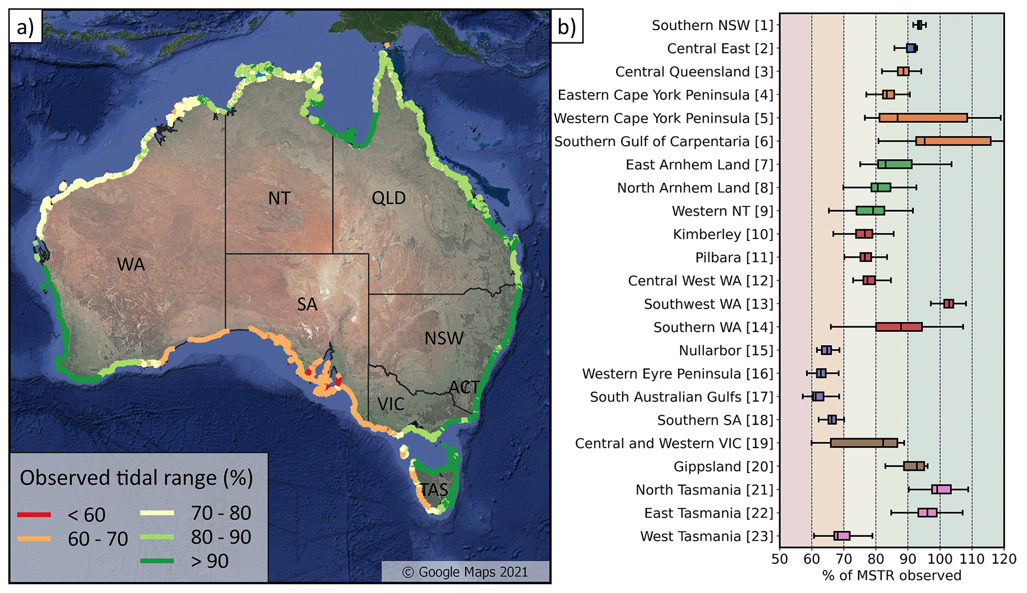
Figure 7 Observed tidal range by the satellite-derived shorelines. Panel (a) maps the % of the MSTR that is observed at each beach and (b) shows the distribution of that metric across the 23 coastal regions.

Vos et al. (2020) previously identified that the performance of the beach-face slope estimation method depends on the signal-to-noise ratio between the accuracy of the satellite-derived shorelines (10–15 m based on the validation in Vos et al., 2019b) and the horizontal extent of the tidal excursion. Thus, the observation of greater uncertainty in slope estimates along the Southwest and Southern WA regions is consistent with the very small tidal range along this coast (<1 m mean spring tidal range, see Supplement Fig. S1a). Another issue affecting the signal-to-noise ratio is the aliasing of the tidal signal by sun-synchronous sensors (i.e. Landsat orbits), which implies that the full tidal range may not always be captured by the satellite imagery (Bishop-Taylor et al., 2019; Eleveld et al., 2014). Figure 7 shows the percentage of the mean spring tidal range (MSTR) that is observed by the satellite-derived shorelines at each beach. This analysis reveals that the SA coastal regions (15–18), which exhibit lower confidence in Fig. 6, have the lowest tide range coverage, with only about 60 %–65 % of the MSTR sampled (Fig. 7a). Thus, along the SA regions that are already microtidal (except inside the gulfs), this aliasing results in only part of the tidal range being observed in the available satellite imagery, further reducing the signal-to-noise ratio and leading to lower-confidence slope estimates.

3.2 An example embayment-scale application

While the previous section focused on the large-scale distribution of beach-face slopes at the continental scale, this dataset can also provide insights into variations in beach-face slope along any individual embayment or beach. To illustrate, Fig. 8a shows beach-face slopes at the transect scale (100 m spacing alongshore) along a single embayment, the Stockton Bight, located in NSW about 150 km north of Sydney. Stockton Bight is the longest beach in NSW, featuring 32 km of south-facing sandy coast backed by a large transgressive dune system (Short, 2020). The beach-face slope data at this site, shown in Fig. 8a, indicates a distinct alongshore gradient, with lower-gradient slopes towards the northern end of the embayment (tan β=0.04) and steeper slopes in the southern end (tan β=0.1). Interestingly, a sediment grain size dataset for the same site is reported by Pucino (2015), with the median swash-zone sand size (D₅₀) at 20 equally spaced sample locations (Fig. 8b) indicating a distinct gradient in grain size along the Stockton Bight embayment. The observed correlation between grain size and beach-face slope that is apparent in Fig. 8 is in agreement with our understanding of this relationship, generally described by a power law (Bujan et al., 2019). This example demonstrates that this continent-wide dataset can also be utilised to gain insights into the alongshore variability of beach-face slopes (and, potentially, grain size distribution) along individual beaches and embayments, informing present-day coastal management and planning.

Figure 8 Embayment-scale gradient in beach-face slopes and sediment grain size. (a) Beach-face slope estimates along 100 m-spaced cross-shore transects along the Stockton Bight embayment. (b) Figure taken from Pucino (2015) displaying the spatial distribution of median grain size (D₅₀) for 20 sand samples along the embayment. D₅₀ values are in microns and have been interpolated using the inverse-weighted distance and discretised into seven quantiles.

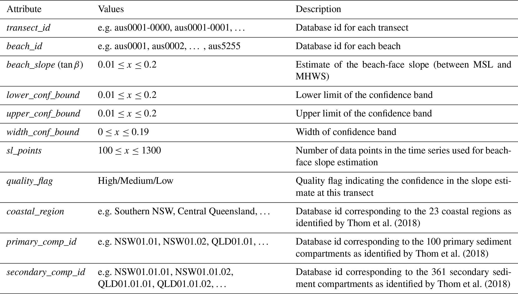
Table 1 Description of data fields for the beach-face slope dataset at the transect scale.

3.3 Dataset description

The data presented above are made available as two geospatial layers (GeoJSON files): one providing the beach-face slope estimates on a transect basis (100 m alongshore spacing) and the second providing the estimates averaged over each individual beach. Tables 1 and 2 describe the attributes of each layer, respectively.

At the transect scale (Table 1), the beach-face slope and confidence bands are accompanied by relevant metadata such as the number of shoreline points used to estimate the beach-face slope, the sediment compartment/region in which the transect is located, and a database id for the transect. A confidence flag (high/medium/low) is associated with each estimate, as is illustrated in Fig. 6.

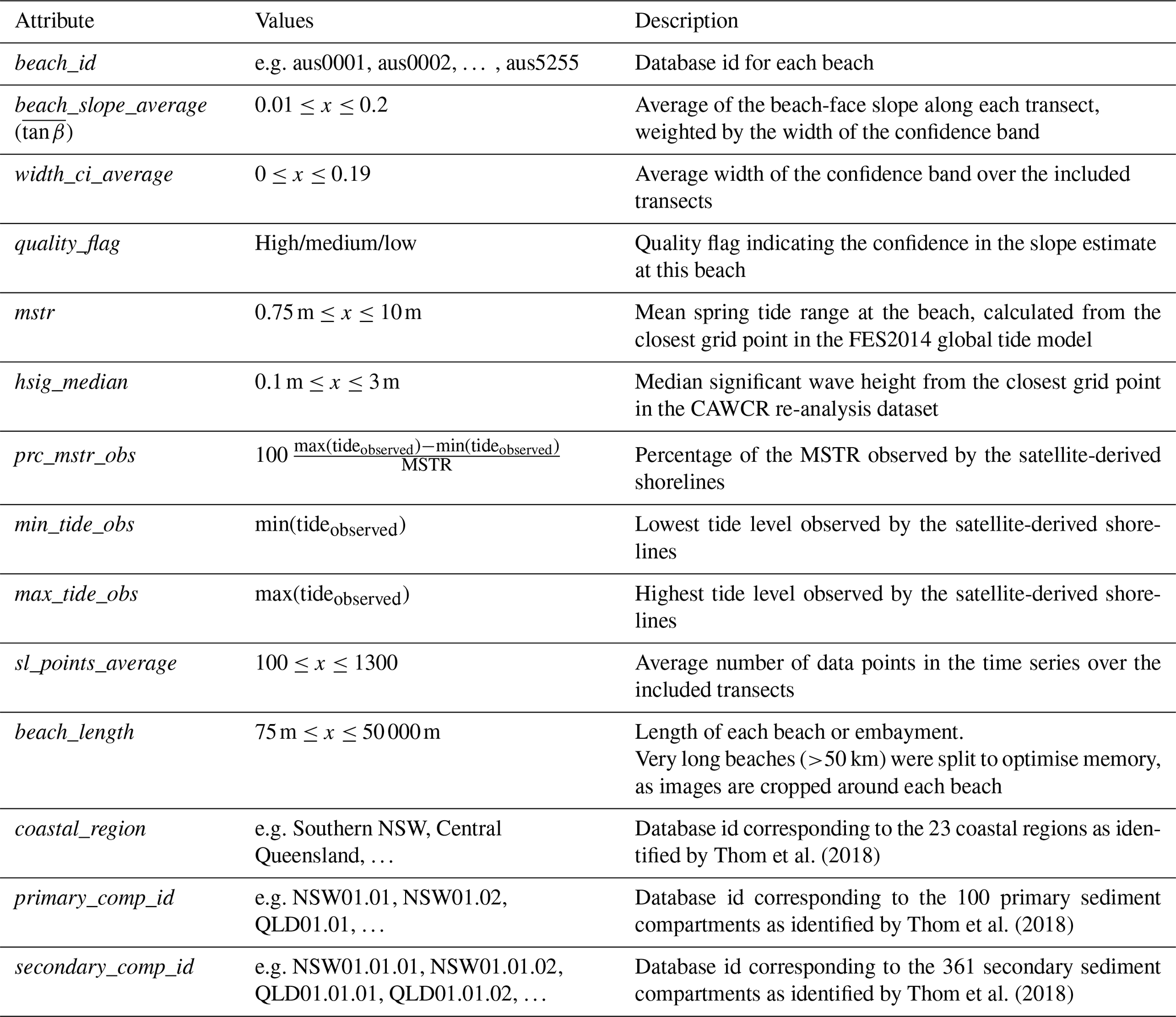
At the beach scale (Table 2), the alongshore-averaged slope weighted by the width of the confidence interval is provided for each individual beach, and is associated with a confidence flag (high/medium/low) based on the alongshore-averaged width of the confidence band. Relevant metadata at the beach scale include the mean spring tide range (MSTR), median significant wave height (Hsig), percentage of observed tide range, minimum observed tide level, maximum observed tide level, and beach length.

Table 2 Description of data fields for the beach-face slope dataset at the individual beach scale.

To assist users of Australia's national sediment compartment framework (Fig. 5), the distribution of beach-face slopes in each sediment compartment is provided in the Supplement at both the primary (Supplement Fig. S3) and secondary (Supplement Fig. S4) levels. Geospatial layers containing the primary and secondary compartments are also included in the dataset and displayed in Supplement Fig. S2.

4 Discussion

This new beach-face slope dataset provides full coverage of the Australian sandy coast, with beach-face slope estimates for 132 000 transects spaced every 100 m and extending along 13 200 km of coast. By focusing on the beach-face slope (defined between the MSL and MHWS), it complements an existing dataset (Athanasiou et al., 2019) of nearshore slopes that are defined for the lower beach profile (between the MSL and the depth of closure). While the nearshore slopes can be used to transform offshore wave parameters to the nearshore (see Fig. 1), the beach-face slope is necessary to predict the elevation of wave run-up and the total swash excursion at the shoreline, which is used in most standard wave run-up formulations (e.g. Stockdon et al., 2006). Consequently, this beach-face slope dataset is an important step towards improving predictions of wave run-up and potential inundation hazards along the Australian coast (O'Grady et al., 2019). Additionally, coastal flood warning systems (e.g. Doran et al., 2015; Leaman et al., 2021; Stokes et al., 2019) often rely on a measure of the uncertainty associated with the input parameters to provide meaningful predictions with a margin of error. In that regard, the confidence bands associated with the beach-face slope estimates in this dataset can be used to propagate the uncertainty into the wave run-up equations and generate ensemble forecasts of total run-up elevation and swash excursion.

As identified in a previous validation at eight diverse sites (Vos et al., 2020), this dataset provides a good estimate of the “typical” or long-term average beach-face slope obtained from 20 years of Landsat imagery. It is recognised, however, that the beach-face slope can vary quite substantially through time, particularly for microtidal intermediate beaches (such as those found in SE Australia), where the beach often rapidly transitions between morphodynamic beach states (Wright and Short, 1984). While estimating this temporal variability is challenging when using the described method with the historic Landsat data (as undertaken here), new satellite remote sensing capabilities may make this a future possibility. For example, by combining satellite missions such as Landsat and Sentinel-2 (5 d revisit at the Equator) with Planet's CubeSat imagery (Kelly and Gontz, 2019), it might be possible to significantly increase the sampling frequency of shoreline observations. This higher-frequency data would enable the use of a narrower time window in which beach-face slopes are estimated, potentially opening up the possibility of estimating the temporal variability in beach-face slopes at different timescales (e.g. inter-annual and seasonal).

While the focus of this dataset is on the Australian coastline, the generic nature of the method and the global extent of Landsat imagery mean that such a dataset could, theoretically, also be reproduced elsewhere. It is important to note, however, that the density of Landsat coverage is not consistent globally (Wulder et al., 2016) and that Australia (along with North America and eastern China) has some of the highest coverage in terms of image density. Additionally, the Australian continent is characterised by a relatively low mean cloud frequency (Wilson and Jetz, 2016), which means that a lower proportion of optical images are hindered by clouds. Other areas with sparser Landsat coverage and/or a higher cloud frequency may not have the same temporal depth of shoreline observations, which could hinder the applicability of this method in some regions.

5 Code availability

The source code to map satellite-derived shorelines from Landsat imagery (CoastSat) is available at https://doi.org/10.5281/zenodo.2779293​​​​​​​ (Vos, 2021a). The source code to estimate beach-face slopes from satellite-derived shorelines and modelled tides (CoastSat.slope) is available at https://doi.org/10.5281/zenodo.3872442 (Vos, 2021b).

6 Data availability

​​​​​​​The continental-scale beach-face slope dataset described in this paper (Sect. 3.3) is available in the following Zenodo data repository: https://doi.org/10.5281/zenodo.5606216 (Vos et al., 2021).

7 Conclusion

This study presents a new dataset of beach-face slopes for the Australian coastline derived from a newly available remote sensing technique. The dataset covers a total of 13 200 km of sandy coast and provides an estimate of the beach-face slope from mean sea level (MSL) to mean high water spring (MHWS) every 100 m alongshore. Based on the width of the confidence band around each slope estimate, it was found that 56 % of the continental-scale dataset can be classified as high confidence, 23 % as medium confidence, and 21 % as low confidence.

The dataset offers a unique view of large- to local-scale scale features in beach-face slope variability, providing data for regions with no in situ observational coverage. This new data availability opens up many interesting applications in coastal sciences and engineering, including:

• i.

  estimates (with confidence bands) of the beach-face slope parameter, which is needed to predict wave run-up in coastal inundation forecasting systems (O'Grady et al., 2019)

• ii.

  enhancing the understanding of large-scale geologic factors that contribute to the distribution of beach-face slopes and sediment grain sizes (Bujan et al., 2019; Short, 2020)

• iii.

  informing coastal management and planning at the embayment scale.

The data are available in a simple format that can be readily imported into standard geographical information system software (e.g. QGIS, ArcGIS) or accessed programmatically for use by coastal researchers and end users.