the Creative Commons Attribution 4.0 License.
the Creative Commons Attribution 4.0 License.
 | 15 Mar 2022
Hyperspectral reflectance spectra of floating matters derived from Hyperspectral Imager for the Coastal Ocean (HICO) observations
Using data collected by the Hyperspectral Imager for the Coastal Ocean (HICO) on the International Space Station between 2010–2014, hyperspectral reflectance spectra of various floating matters in global oceans and lakes are derived for the spectral range of 400–800 nm. Specifically, the entire HICO archive of 9411 scenes is first visually inspected to identify suspicious image slicks. Then, a nearest-neighbor atmospheric correction is used to derive surface reflectance of slick pixels. Finally, a spectral unmixing scheme is used to derive the reflectance spectra of floating matters. Analysis of the spectral shapes of these various floating matters (macroalgae, microalgae, organic particles, whitecaps) through the use of a spectral angle mapper (SAM) index indicates that they can mostly be distinguished from each other without the need for ancillary information. Such reflectance spectra from the consistent 90 m resolution HICO observations are expected to provide spectral endmembers to differentiate and quantify the various floating matters from existing multi-band satellite sensors and future hyperspectral satellite missions such as NASA's Plankton, Aerosol, Cloud, ocean Ecosystem (PACE) mission; Geosynchronous Littoral Imaging and Monitoring Radiometer (GLIMR) mission; and Surface Biology and Geology (SBG) mission. All spectral data are available at https://doi.org/10.21232/74LvC3Kr (Hu, 2021b).
- Article
(1707 KB) - Full-text XML
- BibTeX
- EndNote


Since the debut of the first proof-of-concept Coastal Zone Color Scanner (CZCS, 1978–1986), satellite ocean color missions have evolved from the original goal of mapping phytoplankton biomass and primary production to many other applications. Because of improved spectral resolution and instrument sensitivity, mapping various types of floating matters has also become possible (IOCCG, 2014). These floating matters range from living to non-living, including Sargassum macroalgae, Ulva macroalgae, cyanobacterium Microcystis, cyanobacterium Trichodesmium, dinoflagellate Noctiluca, aquatic plants, brine shrimp cysts, oil slicks, pumice rafts, sea snot, and marine debris, among others (Qi et al., 2020; Hu et al., 2022).
Currently, mapping floating matters using optical remote sensing requires the detection of a spatial anomaly using the near-infrared (NIR) bands and then discrimination of the anomaly by comparing its spectral characteristics with known spectra of floating matters (Qi et al., 2020) or by using ancillary information (e.g., in certain regions a spatial anomaly can only be caused by a certain type of floating algae). Spectral discrimination requires the knowledge of spectral signatures of various floating matters. However, despite scattered laboratory or field measurements of certain types of floating matters, hyperspectral data of these floating matters are mostly unavailable. Although medium-resolution (300 m) sensors such as the Ocean and Land Colour Imager (OLCI) have been used to show spectral variations in floating matters (Qi et al., 2020), the data are not hyperspectral; therefore certain spectral features may have been missed. For example, various pigments (e.g., chlorophyll a, chlorophyll b, chlorophyll c, fucoxanthin, zeaxanthin, phycocyanin, carotenoids) have been found in natural populations of microalgae (i.e., phytoplankton; Bidigare et al., 1990; Bricaud et al., 2004) and macroalgae (e.g., Bell et al., 2015; Wang et al., 2018). These pigments often have narrow absorption and reflectance features that can be missed by multi-band sensors, therefore requiring more spectral bands or hyperspectral data to perform spectroscopic analysis.
Data collected by the Hyperspectral Imager for the Coastal Ocean (HICO) on the International Space Station (ISS) may serve this purpose. HICO has 128 bands covering a spectral range of 353–1080 nm. From its entire mission of 2010–2014, a total of >10 000 scenes have been collected at a spatial resolution of about 90 m, each containing about 512×2000 pixels. On average, only 6 scenes were collected per day around the globe, mostly over land and coastal waters. Because of its stable calibration (Ibrahim et al., 2018) and relatively high signal-to-noise ratios (Hu et al., 2012), deriving hyperspectral surface reflectance of water targets should be feasible. Indeed, after vicarious calibration and atmospheric correction, hyperspectral reflectance data over water have been generated (Ibrahim et al., 2018) and made available through NASA's Ocean Biology Distributed Active Archive Center (OB.DAAC; https://oceancolor.gsfc.nasa.gov, last access: 24 November 2020). However, these data products are not applicable to image pixels containing floating matters due to their interference with the atmospheric correction scheme.
The primary objective of this paper is to derive HICO-based hyperspectral reflectance of various floating matters. This requires customized atmospheric correction and pixel unmixing to account for the small proportion of floating matters within an image pixel. From such derived spectra, a secondary objective is to analyze whether they can be differentiated spectrally. Similarly to the compiled hyperspectral dataset for inherent and apparent optical properties to support future hyperspectral missions such as NASA's Plankton, Aerosol, Cloud, ocean Ecosystem (PACE) mission (Casey et al., 2020), such a dataset for floating matters is expected to help develop or improve algorithms for the PACE mission as well as for the hyperspectral Surface Biology and Geology (SBG) mission currently being planned by NASA (Cawse-Nicholson et al., 2021).
HICO Level-1B (calibrated radiance) data were obtained from the NASA Goddard Space Flight Center (https://oceancolor.gsfc.nasa.gov, last access: 24 November 2020). Of the total collected >10 000 scenes, 9411 were available through this data portal. They were all downloaded, and the following four steps were used to derive spectral reflectance of various floating matters.
Step 1 is to generate quick-look red–green–blue (RGB) and false-color RGB (FRGB) images with Rayleigh-corrected reflectance (Rrc, dimensionless) in three HICO bands using the same methods as in Qi et al. (2020) and in the NOAA OCView online tool (Mikelsons and Wang, 2018). In the FRGB images, a near-infrared (NIR) band is used to represent the green channel, thus making floating matters often appear greenish due to their elevated NIR reflectance. Here, Rrc was generated using the NASA software SeaDAS (version 7.5). Mathematically, it is derived as
where is the at-sensor total radiance after vicarious calibration and adjustment of two-way gaseous absorption (e.g., ozone), Lr is at-sensor radiance due to Rayleigh scattering, Fo is the extraterrestrial solar irradiance, θo is the solar zenith angle, t is the diffuse transmittance from the image pixel to the satellite, to is the diffuse transmittance from the sun to the image pixel, and and are the two-way transmittance due to absorption by atmospheric O2 and H2O, respectively. For simplicity, the wavelength dependency is omitted here.
Step 2 is to determine image slicks through visual inspection of both RGB and FRGB images. Figure 1a shows an FRGB image captured in the central western Atlantic, where an elongated greenish slick is identified.
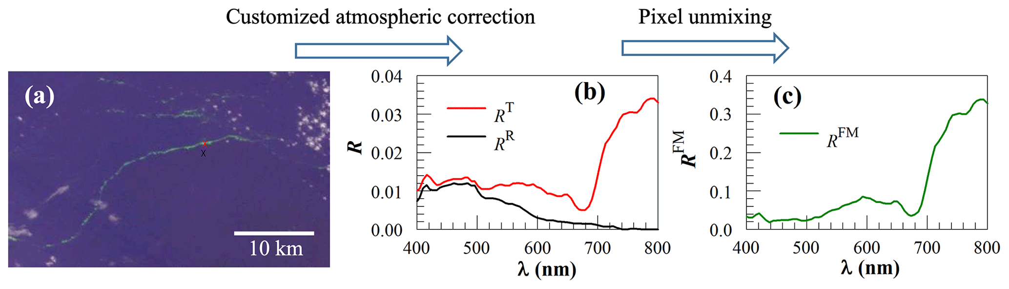
Figure 1Demonstration of how surface reflectance of floating matter (RFM) is derived. (a) FRGB image on 1 July 2012 showing several greenish image slicks in the Amazon River plume. The image covers a region of about 40 km×24 km, with the target (6.65914∘ N, 51.2395∘ W) and reference (6.64847∘ N, 51.2411∘ W) pixels marked with a red × and a black ×, respectively. (b) Their corresponding RT and RR, with the latter derived from SeaDAS and the former derived from a nearest-neighbor atmospheric correction. (c) RFM derived from RT and RR using Eq. (4), with χ being estimated to be 10 %.
Step 3 is to derive surface reflectance (R, dimensionless) of both the slick pixels (i.e., those containing floating matters) and nearby water pixels. While the latter is straightforward because R at each pixel is a standard output of the SeaDAS software, the former is problematic because standard atmospheric correction in SeaDAS fails over floating matters due to their elevated NIR reflectance. Such elevated NIR reflectance violates the atmospheric correction assumptions (i.e., negligible reflectance in the NIR or fixed relationships between the red and NIR wavelengths) for slick pixels. Therefore, a nearest-neighbor atmospheric correction (Hu et al., 2000) was used to estimate the R of the slick pixels. Specifically, from the SeaDAS output of Rrs, we have
where Rrs is the surface remote sensing reflectance (sr−1), Ra is the at-sensor aerosol reflectance (and reflectance due to aerosol–molecule interactions as well as due to sun glint and whitecaps). The difference between R and Rrc in Eqs. (2) and (1), respectively, is the removal of Ra in Eq. (2). Estimation of Ra at each pixel represents the “core” of any atmospheric correction scheme. The SeaDAS estimation of Ra is valid over water pixels but not valid over the slick pixels. Therefore, Ra over water pixels was used as a surrogate to represent Ra over the nearby slick pixels, from which R over slick pixels was derived. This is why such an approach is called “nearest-neighbor” atmospheric correction (Hu et al., 2000). In this context, the slick pixel is called the “target” and the nearby water pixel is called the “reference”. Their surface reflectances are called RT and RR, respectively. Figure 1b shows examples of RT and RR.
The final step, Step 4, is to perform spectral unmixing of RT. This is because floating matters often cover only a small portion of a pixel (Hu, 2021a). In this step, the derived RT from Step 3 is assumed to be a linear mixture of two endmembers, floating matter (RFM) and water (RW):
Here, χ is the subpixel portion of floating matter which can vary between 0.0 % and 100 % and RW is assumed to be RR. Then, the final product, RFM, is derived as
On the right-hand side of Eq. (4), the only unknown is χ. In practice, assuming RFM at 750 nm ≈0.3 as revealed by independent measurements of floating macroalgae (Hu et al., 2017; Wang et al., 2018), χ is estimated through linear unmixing as
Here, with RT(754) varying between RR(754) and 0.3, χ ranges between 0.0 % and 100 %. Plugging this mixing ratio into Eq. (4) will derive RFM. Figure 1c shows the example of how RFM is derived from RT and RR of Fig. 1b once they are known from Step 3, with χ being estimated to be 10 %.
Once RFM is derived, a spectral angle mapper (SAM) index (Kruse et al., 1993) was used to determine whether different floating matters were spectrally different. The SAM approach was used because it is based on spectral shape only. An SAM is the angle between two spectral vectors, defined as in Kruse et al. (1993):
Here, x and y represent two spectral vectors with the ith band from 1 to N. An SAM of 0∘ indicates identical spectral shapes between x and y regardless of their difference in magnitudes, while an SAM of 90∘ indicates completely different spectral shapes. An SAM of indicates that the two spectra are very similar (Garaba and Dierssen, 2018).
The approach above was applied to the visually identified image slicks to derive RFM(λ). These include (1) Sargassum fluitans and S. natans in the Atlantic (including the Caribbean Sea and Gulf of Mexico); (2) Ulva prolifera in the western Yellow Sea (near Qingdao, China); (3) kelp in the South Atlantic; (4) Trichodesmium around Australia, in the Gulf of Mexico and Persian Gulf, in the South Atlantic Bight, in the Bay of Bengal, and near Hawaii and the island of Pagan (middle Pacific); (5) cyanobacteria of Microcystis in Lake Taihu, Lake of the Woods, and Lake Victoria; (6) red Noctiluca scintillans (RNS) in the East China Sea and coastal waters off Japan; (7) brine shrimp cysts in the Great Salt Lake; (8) oil slicks in the Gulf of Mexico; (9) whitecaps (foam) in the Arabian Sea, Caspian Sea, and Bohai Sea; (10) ice in Lake Baikal; and (11) some unknown algae features. For convenience, they are grouped into four figures: Fig. 2 for macroalgae (Sargassum, Ulva, and kelp), Fig. 3 for microalgae (Trichodesmium; Microcystis; red Noctiluca scintillans, or RNS), Fig. 4 for organic particles and ocean/lake bubbles, and Fig. 5 for known and unknown algae scums.
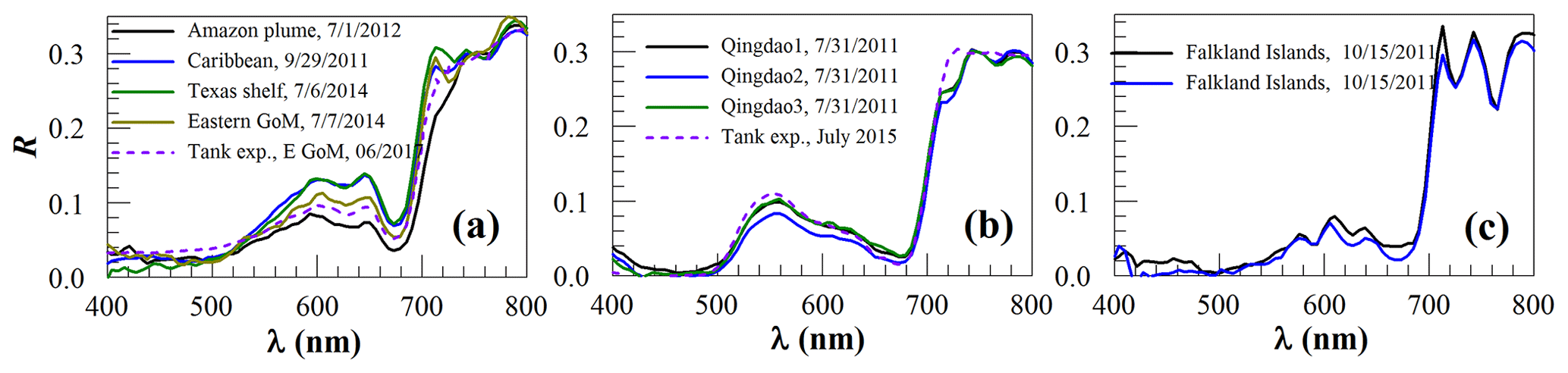
Figure 2Surface reflectance (R, dimensionless) of macroalgae: (a) pelagic Sargassum fluitans and S. natans, (b) Ulva prolifera, (c) kelp. The dashed lines in (a) and (b) denote R from water tank experiments of Wang et al. (2018) and Hu et al. (2017), respectively. GoM denotes the Gulf of Mexico. Where full dates are given in figures, they are formatted as month/day/year.
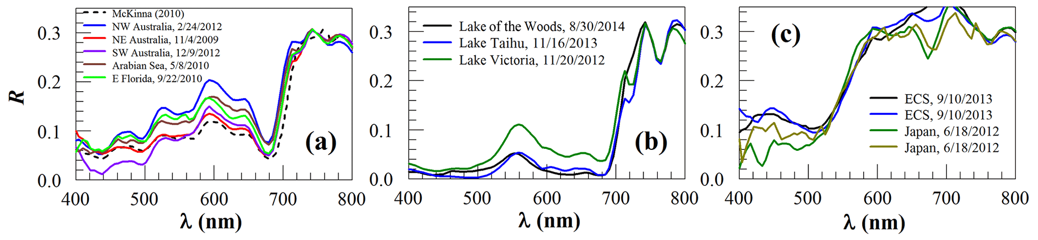
Figure 3Surface reflectance (R, dimensionless) of floating scums of microalgae: (a) Trichodesmium, (b) Microcystis, (c) red Noctiluca near the Yangtze of the East China Sea (ECS) and in Sagami Bay of Japan. The dashed line in (a) denotes field-measured R by McKinna (2010).
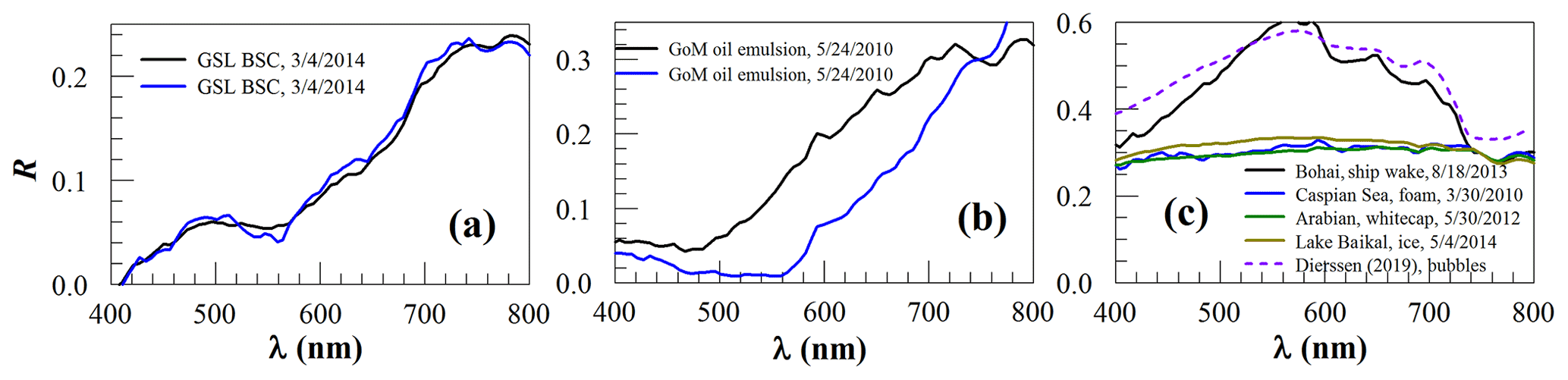
Figure 4Surface reflectance (R, dimensionless) of various floating materials: (a) brine shrimp cysts in the Great Salt Lake (GSL BSC); (b) emulsified oil from the Deepwater Horizon oil spill in the Gulf of Mexico (GoM); and (c) ship wake, sea-foam, whitecaps, and ice. The dashed line in (c) denotes submersed bubbles measured by Dierssen (2019), which is similar to the ship wake spectrum. Note the similarity among other spectra.
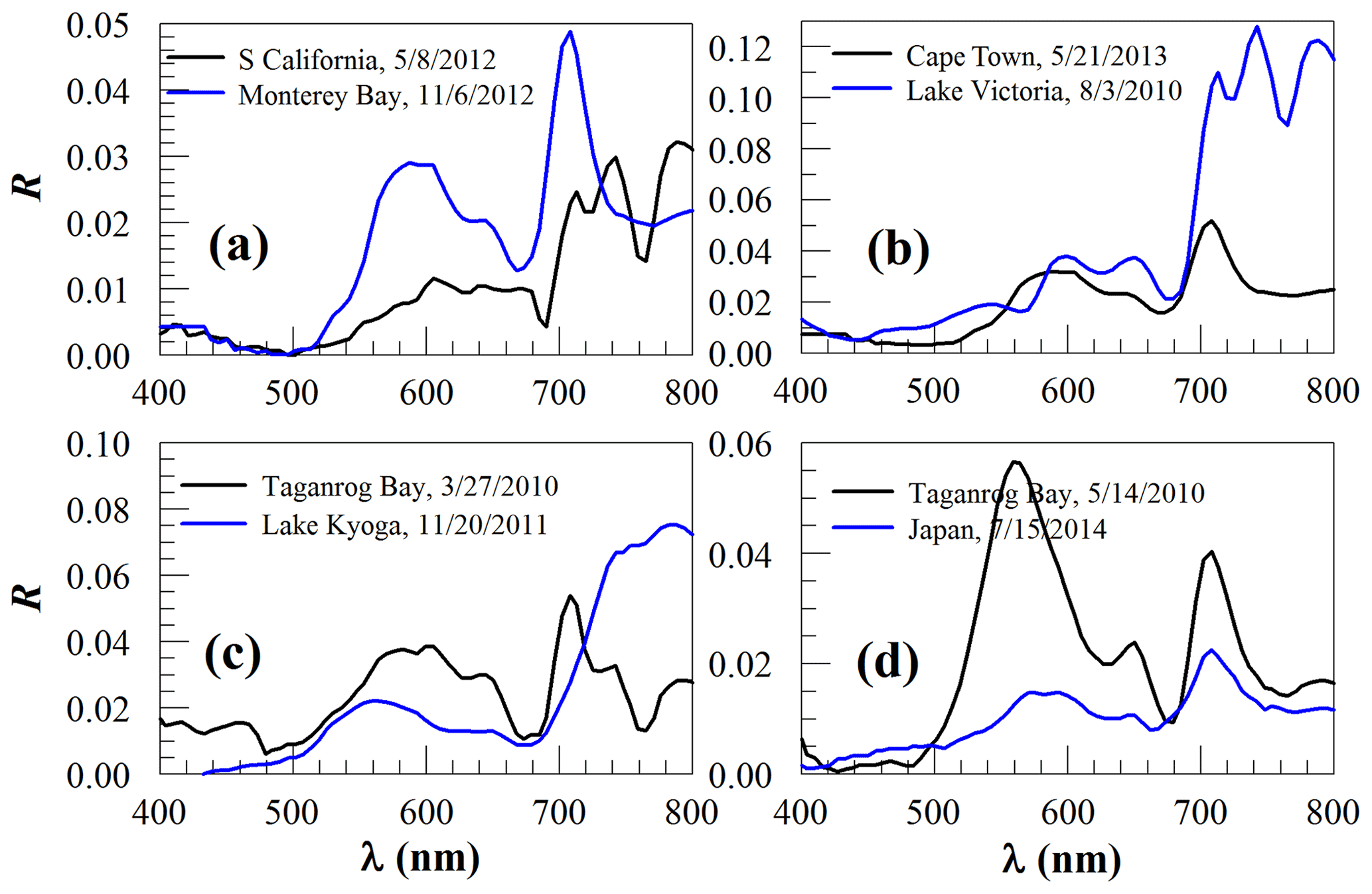
Figure 5Surface reflectance (R, dimensionless) of known and unknown algae scums. (a) Blooms off southern California and in Monterey Bay that are thought to be Lingulodinium polyedrum (Cetinic, 2009) and Akashiwo sanguinea (Jessup et al., 2009), respectively. (b) Blooms of unknown types of algae off Cape Town (South Africa) and in Lake Victoria, both likely to be dinoflagellates. Note the different spectra shape of the Lake Victoria bloom as compared with the cyanobacterial bloom in the same lake (Fig. 3b). (c) Blooms of unknown types of algae in Taganrog Bay and Lake Kyoga. (d) Blooms of unknown types of algae in Taganrog Bay (note the difference from Fig. 5c) and in Japanese coastal waters.
Of all spectra presented in Figs. 2–4, one common feature for all floating macroalgae and microalgae (except red Noctiluca) is the red-edge reflectance (i.e., the sharp increase from about 670 nm to the NIR wavelengths). Such a common feature is due to both chlorophyll a absorption around 670 nm and high reflectance in the red and NIR wavelengths due to macroalgae mats or microalgae scums (Kazemipour et al., 2011; Launeau et al., 2018). The lack of such a red-edge feature in some of the red Noctiluca reflectance spectra (Fig. 3c) is possibly due to the lack of chlorophyll a pigment because red Noctiluca is heterotrophic (i.e., it does not contain pigments unless it feeds on other algae). Other than the common red-edge reflectance, the contrasting spectral shapes of the various types of floating macroalgae and microalgae are due to their different pigment compositions (see below). In contrast, the non-living floating matters do not show red-edge reflectance or other pigment-induced spectral features in the visible wavelengths (Fig. 4). In Fig. 5, in addition to pigment absorption, high scattering due to high concentrations of algae particles together with sharp increases in water absorption from the red to the NIR wavelengths leads to the local reflectance peak around 700 nm (Fig. 5), and, depending on the particle concentrations, the peak wavelength may be slightly shifted, for example from 700 to 710 nm.
4.1 Uncertainties in the derived RFM
There are several assumptions used in the nearest-neighbor atmospheric correction and spectral unmixing (Eq. 4). Violations of these assumptions will cause errors in the derived RFM spectra. For example, if the atmosphere over the floating-matter pixel is different from over the nearby water, the nearest-neighbor atmospheric correction may not be applicable. In practice, however, because the target and reference pixels are very close (<1 km), such a violation is unlikely. In Step 4, the water within the floating matter (FM)-containing pixel is assumed to be the same as the nearby water. Because of the close proximity of the two pixels, this assumption should be valid for most cases unless the FM-containing pixel is at an ocean front where different water masses converge. The departure of RFM(754) from the assumed 0.3 will also lead to errors in the estimated χ (and therefore RFM). However, as long as RW (i.e., RR) in Eqs. (4) and (5) is ≪RFM, the shape of RFM is still retained, although the magnitude departs from the “truth” in proportion to the departure of RFM(754) from 0.3. Indeed, the condition of RW≪RFM can be satisfied for λ >600 nm for most floating matters unless the water is extremely turbid. Even for turbid waters, for certain floating matters where RFM is elevated at λ>530 nm (e.g., red Noctiluca, brine shrimp cysts, ice), the shape of the derived RFM should still be valid for λ>530 nm. Indeed, when RW is ≪RFM, even a simple subtraction of Rrc or top-of-atmosphere radiance between the target pixel and reference pixel, as demonstrated in Gower et al. (2006), may retain the spectral shapes of floating matters.
Another uncertainty source can come from the assumption of linear mixing between floating matters and water (Eq. 3). For macroalgae, linear mixing up to the reflectance saturation level has been shown in laboratory experiments (Hu et al., 2017; Wang et al., 2018). As long as the macroalgae stay on the very surface of the water (as opposed to being submerged under the surface), this assumption should be valid not just for macroalgae but for all floating matters. For the same reason, if certain portions of kelp are submerged in water, large uncertainties may result from the linear unmixing scheme. Under high-wind conditions, the strong mixing may result in submerged algae (especially for microalgae), thus violating the linear mixing rule. However, the cases presented in Figs. 2–5 were selected very carefully to avoid high wind speed (>5 m s−1, where wind speed was obtained from the National Centers for Environmental Prediction). Therefore, such mixing-induced uncertainties are unlikely.
Additional uncertainties may come from the HICO radiometric calibration, which affects Rt and all derivative products. Through the use of the Marine Optical Buoy (MOBY) and other clear-water sites, HICO has been calibrated vicariously (Ibrahim et al., 2018), which has resulted in significant improvements in the retrieved Rrs over water as compared with data without vicarious calibration. However, after the vicarious calibration, while the spectral shape of Rrc over water appears correctly, the shape of ΔRrc over land appears to be biased low at λ>800 nm. Without vicarious calibration, the opposite is observed. This is possibly due to the non-linear effects in the detector response to incoming light, and currently there appears no reliable way to address this issue (Amir Ibrahim, personal communication, 2021). Similarly, calibration for λ<450 nm may be subject to larger errors than for λ between 450 and 800 nm. Therefore, RFM in the range of 800–900 nm is omitted here, and interpretation of 400–450 nm also requires more caution. Similarly, the spectral wiggling between 700 and 800 nm (e.g., Fig. 3b) appears to come from residual errors in correcting water vapor absorption and oxygen absorption in the atmosphere. Therefore, although the spectral wiggling does not affect the overall shape of the red-edge reflectance, it may not be used for algorithm development to discriminate floating-matter types.
Indeed, with all these possible sources of uncertainty, such HICO-derived RFM can still be used for spectral discrimination of different floating matters without ambiguity, as shown below.
4.2 Implications for spectral discrimination
Spectral discrimination can be performed through either visual inspection or the use of a certain type of similarity index (e.g., SAM, Eq. 6). Here, results of the SAM analysis are presented in Table 1, followed by descriptions of visual inspection to interpret the spectral similarity or difference. Because nearly all floating algae show typical red-edge reflectance, discrimination of different algae types is focused on wavelengths <670 nm. To discriminate floating algae from non-living floating matters (e.g., marine debris), on the other hand, the inclusion of 670 nm is critical. Furthermore, because HICO data are noisy for wavelengths <450 nm, the SAM calculation was restricted to 450–670 nm for most RFM spectra of Figs. 2–4.
Table 1Spectral angle mapper values (degrees) between different floating matters for the spectral range of 450–670 nm, derived from the HICO-derived and field-measured spectra shown in Figs. 2–4. An SAM of 0∘ indicates an identical spectral shape, while an SAM of 90∘ indicates a completely different spectral shape. Sarg: Sargassum fluitans and S. natans; Ulva: Ulva prolifera; Tricho: Trichodesmium; Micro: Microcystis; RNS: red Noctiluca scintillans; BSCs: brine shrimp cysts. Because all floating algae show similar red-edge reflectance with a reflectance trough around 670 nm, the exclusion of wavelengths of >670 nm is to reduce the similarity among different types of floating algae. Bold font indicates strong similarity (SAM ).

Table 1 shows the SAM results for three types of macroalgae (Sargassum, Ulva, kelp), three types of microalgae (Trichodesmium; Microcystis; red Noctiluca scintillans, or RNS), and one type of organic matter (brine shrimp cysts, or BSCs). Here, unless noted, Sargassum refers to Sargassum fluitans and S. natans (dominant pelagic type in the Atlantic Ocean) and Ulva refers to Ulva prolifera (dominant pelagic type in the Yellow Sea). For the same floating matter, if field-based RFM is available, then it is used as the reference; otherwise the mean HICO-derived RFM is used as the reference. For the SAM between different floating matters, all HICO-derived RFM values from both types are used (e.g., 4 Sargassum RFM values of Fig. 2a and 3 Ulva RFM values of Fig. 2b are used to calculate 12 SAM values), with their means and standard deviations listed in Table 1.
For each type of floating matter, HICO-derived RFM is very similar to either field-measured RFM or the floating matter's mean RFM, with SAM . In contrast, the SAM between different floating matters is always . These results suggest that, if these floating matters represent all that can be found in natural waters, they can be differentiated through spectroscopy analysis without any other ancillary information (e.g., knowledge of local oceanography or dominant floating algae type). This is despite the possible uncertainties in their reflectance magnitude, as discussed above. In the natural environments, however, there may be other types of floating algae whose spectral shapes may be similar to Sargassum fluitans and S. natans (e.g., either Sargassum horneri in the East China Sea or other brown algae) or Ulva prolifera (e.g., other green algae). Therefore, some form of ancillary information in addition to spectroscopy is still required in order to differentiate floating algae types.
The results from the SAM table can also be explained through visual inspection and interpretation of the spectral shapes, as discussed below.
From Fig. 2, it is clear that although the three types of macroalgae all share the same red-edge reflectance in the NIR, they have different spectral shapes in the visible wavelengths. Unlike the Ulva reflectance with a local peak around 560 nm, the spectral shapes of Sargassum reflectance resemble those of typical brown algae where the local reflectance trough around 625 nm is induced by chlorophyll c absorption and the low reflectance below ∼520 nm is due to carotenoid pigment absorption. These characteristics make it easy to distinguish Sargassum from Ulva (, Table 1). On the other hand, it appears more difficult to spectrally discriminate Sargassum from kelp because they both have reflectance peaks around 600–645 nm and because they also share a common reflectance trough around 625 nm. However, considering Sargassum is moving in the ocean while kelp is fixed in location, they can be separated using sequential images. Even from a single image, when most visible wavelengths are used, Sargassum and kelp can still be spectrally discriminated (, Table 1). Within the group of Sargassum spectra (Fig. 2a), there is some variability in the magnitude between 560–700 nm. It is unclear what caused such variability, although it could be due to changes in the carbon-to-chlorophyll ratio in Sargassum of different environment, as observed from kelp (Bell et al., 2015). Such a variability, however, would not impact the spectral discrimination of Sargassum from other floating matters, as the SAM between Sargassum spectra is , much lower than between Sargassum and any other types of floating matters (Table 1).
Similarly to the macroalgae, the microalgae scums also show elevated NIR reflectance (Fig. 3), and their spectral shapes in the visible wavelengths makes it straightforward to distinguish between kinds () and also straightforward to distinguish them from macroalgae (). One exception may be the cyanobacterial scums (blue-green algae blooms) (Fig. 3b) as they show a reflectance peak around 550 nm, similarly to Ulva (Fig. 2b). However, reflectance around 550 nm is nearly symmetric for cyanobacterial scums but asymmetric for Ulva. There is also a local reflectance trough around 625 nm for cyanobacterial scums due to absorption of phycocyanin, but such a trough is lacking in the Ulva spectra. Such a characteristic makes it possible to differentiate between the two even without a priori knowledge of the ocean or lake environment, as the SAM between the two groups is ∼16.8∘ (Table 1). What is interesting is that within each class, either Trichodesmium or Microcystis, although the spectral shape is nearly identical from different spectra (), there is substantial variability in the magnitude in the visible wavelengths, which might be due to changes in their carbon-to-chlorophyll ratios (Behrenfeld et al., 2005). Furthermore, the spectral-wiggling features between 450 and 660 nm in Fig. 3a are due to Trichodesmium-specific pigments such as phycourobilin, phycoerythrobilin, and phycocyanin that absorb light strongly at 495, 550, and 625 nm, respectively (Navarro Rodriguez, 1999). These features are unique to Trichodesmium scums, which makes it straightforward to develop classification algorithms once certain spectral bands are available to capture these features (e.g., Hu et al., 2010).
Of all the microalgae scums of Fig. 3, the spectral shapes of red Noctiluca (Fig. 3c) appear different from all others, but they show the same characteristics as those reported from the limited field measurements (Van Mol et al., 2007): a sharp, featureless increase from ∼520 to ∼600 nm. This unique spectral shape makes RNS different from all other floating matters (, Table 1). The difference within this group is that the spectra from Sagami Bay off Japan show reflectance troughs around 670 nm. Because red Noctiluca is known to feed on other algae, it is speculated that the 670 nm trough is due to chlorophyll pigments of the consumed algae. Once more hyperspectral data are available in the future to test this hypothesis using field data, this characteristic may be used to study how red Noctiluca interacts with other algae. On the other hand, once more hyperspectral data are available in the future, it is also possible to test whether other algae (e.g., Mesodinium rubrum; Dierssen et al., 2015), once they have formed surface scum, have similar spectral shapes to those of red Noctiluca.
The non-algae floating matters in Fig. 4 show spectral characteristics different from both macroalgae and microalgae; for example they lack the typical red-edge reflectance of vegetation and lack typical spectral variations in the visible wavelengths due to pigment absorption. Within this group, the organic matter of BSCs (Fig. 4a) and emulsified oil (Fig. 4b) show some degrees of similarity as they also have monotonic reflectance increases from a wavelength between 500–560 to at least 740 nm. The difference between them is that BSC reflectance always starts to increase at ∼560 nm with an inflection wavelength of ∼640 nm, while reflectance of oil emulsions start to increase at variable wavelengths without any inflection between 560–740 nm. Indeed, the infection at ∼640 nm appears to be a common feature between BSC slicks and coral spawn slicks (Yamano et al., 2020). In contrast, depending on the oil emulsion state, oil emulsion may have different spectral characteristics (Lu et al., 2019), suggesting that there is no fixed “endmember” spectra for oil spills.
The inorganic “particles” (i.e., water bubbles, ice) also have distinctive spectral shapes. The examples in Fig. 4c indicate that submersed bubbles from ship wakes are similar in terms of spectral shapes, but all others are nearly identical in their lack of any narrow-band spectral features. Rather, foams, whitecaps, and ice all show flat reflectance spectral shapes between 400–800 nm that are consistent with in situ measurements of foams (Dierssen, 2019). The lack of narrow-band spectral features is similar to marine debris (Garaba and Dierssen, 2020). Such a similarity will make detection of marine debris very difficult, especially around ocean fronts because these are where surface materials tend to aggregate and foams also tend to form.
In addition to the spectra of Figs. 2–4 that can be well recognized, HICO also showed reflectance spectra that are difficult to discriminate from spectroscopy alone, as shown in Fig. 5. Without a known reflectance library, one can only speculate what algae type could be responsible for the algae scum spectra from some ancillary information in the literature. For example, the often-reported blooms of Lingulodinium polyedrum and Akashiwo sanguinea in coastal waters off southern California and in Monterey Bay, respectively, may show spectral shapes of those in Fig. 5a when they are heavily concentrated in surface waters. Inference may also be made for other cases once similar ancillary information is available. Even when such information is absent, one can still rule out some possibilities simply based on the spectral shapes. For example, the reflectance spectrum in Fig. 5b from Lake Victoria cannot be from cyanobacteria that has been often reported in this lake (Fig. 3b), but it is most likely from a dinoflagellate bloom, as blooms of other algae types have also been reported in this lake (Haande et al., 2011). Likewise, the different spectra from the same Taganrog Bay in Fig. 5c and d suggest different algae types. Clearly, although cyanobacterial blooms have been reported in many lakes, without spectral diagnosis one cannot simply jump to the conclusion that a freshwater bloom is caused by a certain type of cyanobacterium.
4.3 Implications for current and future satellite missions
Because HICO is a pathfinder sensor that collected only a limited number of scenes, not all reported floating matters have been captured. For example, no HICO scene appears to have captured pumice rafts, Sargassum horneri, sea snot, or marine debris. Therefore, the spectral reflectance dataset presented here is incomplete. The use of data from other similar pathfinders, for example the DLR Earth Sensing Imaging Spectrometer (DESIS) on the ISS (235 bands from 400–1000 nm, 30 m resolution, 2018–present) and the PRecursore IperSpettrale della Missione Applicativa (PRISMA, 237 bands from 400–2505 nm, 30 m resolution, 2019–present), may complement the spectral data using the same approach presented here (e.g., sea snot reflectance spectra derived from DESIS; Hu et al., 2022). Even in their present form, given the large variety of floating matters presented here, the spectral data may lead to several implications for current and future satellite missions.
First, although all current multi-band sensors can detect floating matters through its elevated NIR reflectance (Qi et al., 2020), the Sentinel-3 Ocean and Land Colour Imager (OLCI) appears to be the best at differentiating spectral shapes in the visible wavelengths because of its 21 spectral bands between 400 and 1020 nm, especially because of its 620 nm band that can be used to differentiate whether an algae scum appears greenish or brownish, thus providing extra information to discriminate algae type in the absence of hyperspectral data.
Second, for the same reason, although only four bands (blue, green, red, NIR) are available on the PlanetScope (Dove) constellation, the recent SuperDove constellation is equipped with four additional bands with one centered at 610 nm and thus may significantly enhance the capacity of the current high-resolution sensors (∼3–4 or 30 m) to differentiate greenish and brownish algae types.
Finally, the Ocean Color Instrument (OCI) on NASA's PACE mission, to be launched in 2023, will be the first of its kind to map global oceans with hyperspectral capacity (5 nm resolution between 340–890 nm, plus seven discrete bands from 940 to 2260 nm) with a nominal resolution of 1 km. Unlike HICO, OCI will cover global oceans and lakes every 1–2 d, thus providing unprecedented opportunities to detect, differentiate, and quantify various types of floating matters. The spectral reflectance data, derived from one sensor (HICO) with a stable calibration, may serve as a consistent dataset to help select the optimal bands for future applications once PACE data become available, for example, through the use of an SAM matrix as demonstrated in Table 1. Likewise, the SBG mission currently being planned by NASA is expected to have hyperspectral capacity between 380 and 2500 nm with a nominal resolution of 30 m (Cawse-Nicholson et al., 2021); such a mission will provide unprecedented opportunity to map various floating matters on a global scale, and the hyperspectral dataset developed here can help develop algorithms before its launch.
All HICO data used in this analysis are available at the NASA Ocean Biology Distributed Active Archive Center (OB.DAAC, https://oceancolor.gsfc.nasa.gov, NASA, 2020a). The data processing software (SeaDAS) can be obtained from the same source, at https://seadas.gsfc.nasa.gov (NASA, 2020b). The derived HICO spectra in digital data form, as shown in the above figures, are available online from the Ecological Spectral Information System (EcoSIS) (http://ecosis.org, last access: 9 March 2022, https://doi.org/10.21232/74LvC3Kr) (Hu, 2021b).
Through customized atmospheric correction and spectral unmixing, hyperspectral reflectance spectra in the visible and NIR wavelengths of various floating matters have been derived from HICO measurements over global oceans and lakes.
The reflectance dataset shows distinguishable spectral shapes between floating algae (macroalgae and microalgae, such as Sargassum fluitans and S. natans, Ulva prolifera, kelp, Microcystis, Trichodesmium, red Noctiluca scintillans) and between floating algae and non-algae floating matters. While the approach may be extended to other pathfinder missions to complement the findings here, the spectral reflectance dataset is expected to help select optimal bands for future hyperspectral satellite missions to differentiate and quantify the various floating matters in global oceans and lakes.
The contact author has declared that there are no competing interests.
Publisher's note: Copernicus Publications remains neutral with regard to jurisdictional claims in published maps and institutional affiliations.
I thank NASA and the US Naval Research Laboratory for providing HICO data, thank Lachlan McKinna for providing field-measured reflectance of Trichodesmium, and thank Heidi Dierssen for providing field-measured reflectance of whitecaps. Patrick Launeau and Qianguo Xing provided useful comments to improve the presentation of this work, and their efforts are appreciated.
This research has been supported by the Earth Sciences Division of NASA (grant nos. 80NSSC21K0422, NNX17AF57G, 80NSSC20M0264, and 80LARC21DA002).
This paper was edited by François G. Schmitt and reviewed by Patrick Launeau and Qianguo Xing.
Behrenfeld, M. J., Boss, E., Siegel, D. A., and Shea, D. M.: Carbon-based ocean productivity and phytoplankton physiology from space, Global Biogeochem. Cy., 19, GB1006, https://doi.org/10.1029/2004GB002299, 2005.
Bell, T. W., Cavanaugh, K. C., and Siegel, D. A.: Remote monitoring of giant kelp biomass and physiological condition: An evaluation of the potential for the Hyperspectral Infrared Imager (HyspIRI) mission, Remote Sens. Environ., 167, 218–228, https://doi.org/10.1016/j.rse.2015.05.003, 2015.
Bidigare, R. R., Ondrusek, M. E., Morrow, J. H., and Kiefer, D. A.: In-vivo absorption properties of algal pigments, Proc. SPIE 1302, Ocean Optics X, 1 September 1990, https://doi.org/10.1117/12.21451, 1990.
Bricaud, A., Claustre, H., Ras, J., and Oubelkheir, K.: Natural variability of phyto- planktonic absorption in oceanic waters: influence of the size structure of algal populations, J. Geophys. Res., 109, C11010, https://doi.org/10.1029/2004JC002419, 2004.
Casey, K. A., Rousseaux, C. S., Gregg, W. W., Boss, E., Chase, A. P., Craig, S. E., Mouw, C. B., Reynolds, R. A., Stramski, D., Ackleson, S. G., Bricaud, A., Schaeffer, B., Lewis, M. R., and Maritorena, S.: A global compilation of in situ aquatic high spectral resolution inherent and apparent optical property data for remote sensing applications, Earth Syst. Sci. Data, 12, 1123–1139, https://doi.org/10.5194/essd-12-1123-2020, 2020.
Cawse-Nicholson, K., Townsend, P. A., and Schimel, D., et al.: NASA's surface biology and geology designated observable: A perspective on surface imaging algorithms, Remote Sens. Environ., 257, 112349, https://doi.org/10.1016/j.rse.2021.112349, 2021.
Cetinic, I.: Harmful algal blooms in the urbanized coastal ocean: An application of remote sensing for understanding, characterization and prediction, PhD thesis, University of Southern California, UMI number 3368500, 239 pp., 2009.
Dierssen, H., McManus, G. B., Chlus, A., Qiu, D., Gao, B.-C., and Lin, S.: Space station image captures a red tide ciliate bloom at high spectral and spatial resolution, Proc. Natl. Acad. Sci. USA, 112, 14783–14787, https://doi.org/10.1073/pnas.1512538112, 2015.
Dierssen, H. M.: Hyperspectral Measurements, Parameterizations, and Atmospheric Correction of Whitecaps and Foam From Visible to Shortwave Infrared for Ocean Color Remote Sensing, Front. Earth Sci., 7, 14, https://doi.org/10.3389/feart.2019.00014, 2019.
Garaba, S. P. and Dierssen, H. M.: An airborne remote sensing case study of synthetic hydrocarbon detection using short-wave infrared absorption features identified from marine-harvested macro- and microplastics, Remote Sens. Environ., 205, 224–235, https://doi.org/10.1016/j.rse.2017.11.023, 2018.
Garaba, S. P. and Dierssen, H. M.: Hyperspectral ultraviolet to shortwave infrared characteristics of marine-harvested, washed-ashore and virgin plastics, Earth Syst. Sci. Data, 12, 77–86, https://doi.org/10.5194/essd-12-77-2020, 2020.
Gower, J., Hu, C., Borstad, G., and King, S.: Ocean color satellites show extensive lines of floating Sargassum in the Gulf of Mexico, IEEE T. Geosci. Remote, 44, 3619–3625, https://doi.org/10.1109/TGRS.2006.882258, 2006.
Haande, S., Rohrlack, T., Semyalo, R. P., Brettum, P., Edvardsen, B., Lyche-Solheim, A., Sørensen, K., and Larsson, P: Phytoplankton dynamics and cyanobacterial dominance in Murchison Bay of Lake Victoria (Uganda) in relation to environmental conditions, Limnologica, 41, 20–29, https://doi.org/10.1016/j.limno.2010.04.001, 2011.
Hu, C.: Remote detection of marine debris using satellite observations in the visible and near infrared spectral range: Challenges and potentials, Remote Sens. Environ., 259, 112414, https://doi.org/10.1016/j.rse.2021.112414, 2021a.
Hu, C.: Floating matter reflectance from HICO, Ecological Spectral Information System (EcoSIS) [data set], https://doi.org/10.21232/74LvC3Kr, 2021b.
Hu, C., Carder, K. L., and Muller-Karger, F. E.: Atmospheric correction of SeaWiFS imagery over turbid coastal waters: a practical method, Remote Sens. Environ., 74, 195–206, https://doi.org/10.1016/S0034-4257(00)00080-8, 2000.
Hu, C., Cannizzaro, J., Carder, K. L., Muller-Karger, F. E., and Hardy, R.: Remote detection of Trichodesmium blooms in optically complex coastal waters: Examples with MODIS full-spectral data, Remote Sens. Environ., 114, 2048–2058, https://doi.org/10.1016/j.rse.2010.04.011, 2010.
Hu, C., Feng, L., Lee, Z., Davis, C. O., Mannino, A., McClain, C. R., and Franz, B. A.: Dynamic range and sensitivity requirements of satellite ocean color sensors: learning from the past, Appl. Opt., 51, 6045–6062, https://doi.org/10.1364/AO.51.006045, 2012.
Hu, C., Qi, L., Xie, Y., Zhang, S., and Barnes, B. B.: Spectral characteristics of sea snot reflectance observed from satellites: Implications for remote sensing of marine debris, Remote Sens. Environ., 269, 112842, https://doi.org/10.1016/j.rse.2021.112842, 2022.
Hu, L., Hu, C., and He, M.-X.: Remote estimation of biomass of Ulva prolifera macroalgae in the Yellow Sea, Remote Sens. Environ., 192, 217–227, https://doi.org/10.1016/j.rse.2017.01.037, 2017.
Ibrahim, A., Franz, B. A., Ahmad, Z., Healy, R., Knobelspiesse, K., Gao, B.-C., Proctor, C., and Zhai, P.-W.: Atmospheric correction for hyperspectral ocean color retrieval with application to the Hyperspectral Imager for the Coastal Ocean (HICO), Remote Sens. Environ., 204, 60–75, https://doi.org/10.1016/j.rse.2017.10.041, 2018.
IOCCG: Phytoplankton Functional Types from Space, in: Reports of the International Ocean-Colour Coordinating Group, No. 15, edited by: Sathyendranath, S., IOCCG, Dartmouth, Canada, ISSN 1098-6030, https://ioccg.org/wp-content/uploads/2018/09/ioccg_report_15_2014.pdf (last access: 8 March 2022), 2014.
Jessup, D. A., Muller, M. A., Ryan, J. P., Nevins, H. M., Kerkering, H. A., Mekebri, A., Crane, D. B., Johnson, T. A., and Kudela, R. M.: Mass stranding of marine birds caused by a surfactant-producing red tide, PLoS ONE, 4, e4550, https://doi.org/10.1371/journal.pone.0004550, 2009.
Kazemipour, F., Méléder, V., and Launeau P.: Optical properties of microphytobenthic biofilms (MPBOM): Biomass retrieval implication, J. Quant. Spectrosc. Ra., 112, 131–142, https://doi.org/10.1016/j.jqsrt.2010.08.029, 2011.
Kruse, F. A., Lefkoff, A. B., Boardman, J. W., Heidebrecht, K. B., Shapiro, A. T., Barloon, P. J., and Goetz, A. F. H.: The spectral image processing system (SIPS) – interactive visualization and analysis of imaging spectrometer data, Remote Sens. Environ., 44, 145–163, https://doi.org/10.1016/0034-4257(93)90013-N, 1993.
Launeau, P., Méléder, V., and Verpoorter, C., Barille, L., Kazemipour-Ricci, F., Giraud, M., Jesus, B., and Le Menn, E.: Microphytobenthos Biomass and Diversity Mapping at Different Spatial Scales with a Hyperspectral Optical Model, Remote Sens., 10, 716, https://doi.org/10.3390/rs10050716, 2018.
Lu, Y., Shi, J., Wen, Y., Hu, C., Zhou, Y., Sun, S., Zhang, M., Mao, Z., and Liu, Y.: Optical interpretation of oil emulsions in the ocean – Part I: Laboratory measurements and proof-of-concept with AVIRIS observations, Remote Sens. Environ., 230, 111183, https://doi.org/10.1016/j.rse.2019.05.002, 2019.
McKinna, L. I. W.: Optical detection and quantification of Trichodesmium spp. within the Great Barrier Reef, PhD thesis, James Cook University, Australia, 312 pp., https://researchonline.jcu.edu.au/15643/ (last access: 8 March 2022), 2010.
Mikelsons, M. and Wang, M.: Interactive online maps make satellite ocean data accessible, Eos, 99, https://doi.org/10.1029/2018EO096563, 2018.
NASA: Ocean Color Data Portal, NASA [data set], https://oceancolor.gsfc.nasa.gov, last access: 24 November 2020a.
NASA: The Official NASA/OB.DAAC Data Analysis Software, NASA [software], https://seadas.gsfc.nasa.gov, last access: 24 November 2020b.
Navarro Rodriguez, A. J.: Optical properties of photosynthetic pigments and abundance of the cyanobacterium Trichodesmium in the eastern Caribbean Basin, PhD Thesis, University of Puerto Rico, Mayaguez (Puerto Rico), 125 pp., Source DAI-B 59/08, 1999.
Qi, L., Hu, C., Mikelsons, K., Wang, M., Lance, V., Sun, S., Barnes, B. B., Zhao, J., and der Zande, D. V.: In search of floating algae and other organisms in global oceans and lakes, Remote Sens. Environ., 239, 111659, https://doi.org/10.1016/j.rse.2020.111659, 2020.
Van Mol, B., Ruddick, K., Astoreca, R., Park, Y., and Nechad, B.: Optical detection of a Noctiluca scintillans bloom, EARSeL eProceedings, 6, 130–137, 2007.
Wang, M., Hu, C., Cannizzaro, J., English, D., Han, X., Naar, D., Lapointe, B., Brewton, R., and Hernandez, F.: Remote sensing of Sargassum biomass, nutrients, and pigments, Geophys. Res. Lett., 45, 12359–12367, https://doi.org/10.1029/2018GL078858, 2018.
Yamano, H., Sakuma, A., and Harii, S.: Coral-spawn slicks: Reflectance spectra and detection using optical satellite data, Remote Sens. Environ., 251, 112058, https://doi.org/10.1016/j.rse.2020.112058, 2020.