Antarctic atmospheric boundary layer observations with the Small Unmanned Meteorological Observer (SUMO)

Between January 2012 and June 2017 a small unmanned aerial system (sUAS), known as the Small Unmanned Meteorological Observer (SUMO), was used to observe the state of the atmospheric boundary layer in the Antarctic. During six Antarctic field campaigns, 116 SUMO flights were completed. These flights took place during all seasons over both permanent ice and ice-free locations on the Antarctic continent and over sea ice in the western Ross Sea. Sampling was completed during spiral ascent and descent flight paths that observed the temperature, humidity, pressure and wind up to 1000 m above ground level and sampled the entire depth of the atmospheric boundary layer, as well as portions of the free atmosphere above the boundary layer. A wide variety of boundary layer states were observed, including very shallow, strongly stable conditions during the Antarctic winter and deep, convective conditions over ice-free locations in the summer. The Antarctic atmospheric boundary layer data collected by the SUMO sUAS, described in this paper, can be retrieved from the United States Antarctic Program Data Center (https://www.usap-dc.org, last access: 8 March 2021). The data for all flights conducted on the continent are available at https://doi.org/10.15784/601054 (Cassano, 2017), and data from the Ross Sea flights are available at https://doi.org/10.15784/601191 (Cassano, 2019).

1 Introduction

The turbulent lower portion of the atmosphere, known as the atmospheric boundary layer, is the part of the atmosphere that interacts directly with the underlying surface. At lower and middle latitudes, atmospheric properties in the boundary layer change diurnally in response to the diurnal cycle of net radiation at the surface. During the day, downwelling shortwave radiation often results in a positive surface radiation budget, surface heating and the development of a convective boundary layer with temperature decreasing with height at a rate of approximately 10 K km⁻¹. At night, longwave radiative cooling from the surface results in surface cooling and the development of a statically stable boundary, often characterized by a surface-based inversion, where temperature increases with height. The presence of clouds or changes in large-scale winds will alter this typical diurnal boundary layer evolution (Stull, 1988).

In the polar regions, a weaker, or absent, diurnal cycle in radiative forcing results in a less pronounced diurnal cycle in boundary layer evolution compared to that observed at lower latitudes, although some locations, such as the McMurdo Dry Valleys, do experience a pronounced diurnal cycle during the austral summer (Katurji et al., 2013). The presence of extensive ice-covered surfaces reduces the amount of solar radiation absorbed at the surface during the day and weakens, or eliminates, the presence of convective boundary layer conditions. During the long polar night, extended periods of radiative cooling at the surface lead to the development of stably stratified boundary layers with strong temperature inversions, although strong winds or clouds can cause the surface inversion to dissipate and well-mixed conditions to develop (King and Turner, 1997; Cassano et al., 2016a; Nigro et al., 2017).

The vast majority of in situ atmospheric observations in the Antarctic are surface observations within the lowest 10 m of the atmosphere with very few observations made above the surface (Summerhayes, 2008). This lack of information on the vertical structure of the atmosphere, even in the lowest tens to hundreds of meters, limits our ability to study the Antarctic boundary layer. Cassano et al. (2016a) provide a summary of Antarctic boundary layer studies that made in situ observations of vertical profiles of atmospheric properties. Antarctic field campaigns from the 1950s to the present have often relied on data collected from meteorological towers that extend up to 50 m above the surface.

More recently, several groups have used unmanned aerial systems (UASs) to observe the Antarctic boundary layer (Cassano, 2014). The British Antarctic Survey was the first to use UASs for Antarctic boundary layer observations with 20 scientific flights conducted in October and December 2007 (Philip Anderson, personal communication, 2013). Cassano et al. (2010, 2016b) and Knuth et al. (2013) describe UAS flights which observed air–sea exchanges in the Terra Nova Bay polynya in the western Ross Sea. The Finnish Meteorological Institute has conducted UAS flights in Dronning Maud Land, Antarctica, at the Aboa research station. Several different UASs were deployed from the RV Polarstern ice breaker in the Weddell Sea during the austral winter of 2013 (Jonassen et al., 2015).

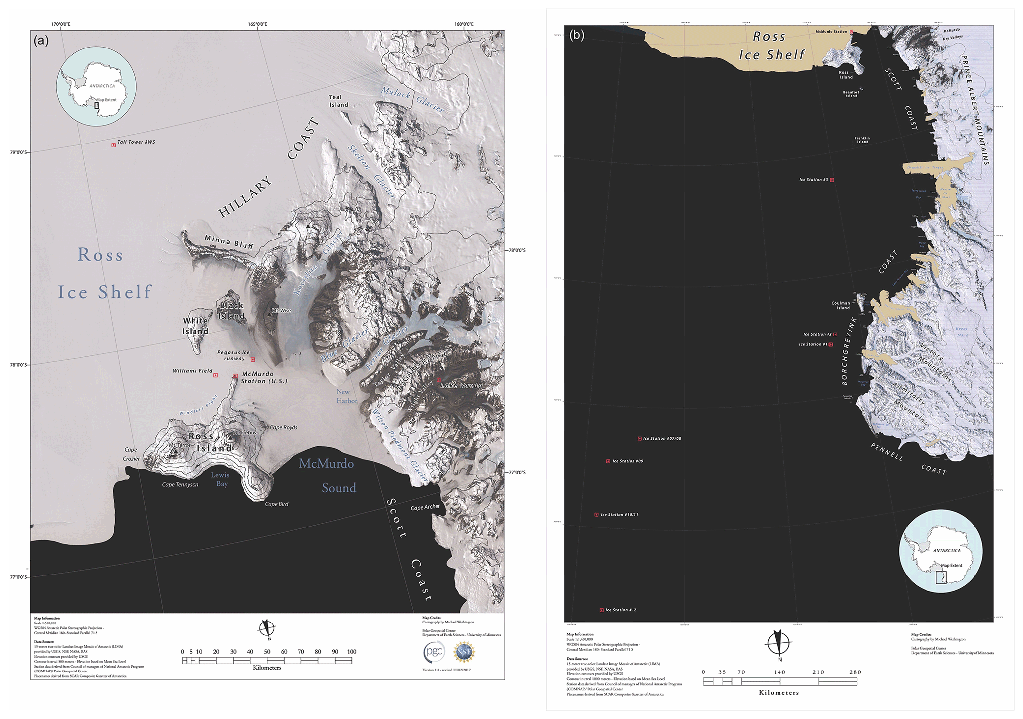
Figure 1 Location of all SUMO sUAS boundary layer flights (red squares) over the Antarctic continent (a) and the Ross Sea (b). Maps prepared by Michael Wethington, Polar Geospatial Center, Department of Earth Sciences, University of Minnesota.

Our research group has used an easily deployed small UAS (sUAS) known as the Small Unmanned Meteorological Observer (SUMO) (Reuder et al., 2009) during six Antarctic field campaigns from 2012 through 2017. These SUMO campaigns have occurred on the Ross Ice Shelf near Ross Island and in the McMurdo Dry Valleys (Fig. 1) in the austral summer and late austral winter into early spring. Austral autumn and winter SUMO flights were conducted as part of the polynyas, ice production and seasonal evolution in the Ross Sea (PIPERS) research cruise in the western Ross Sea from April to June 2017 (Ackley et al., 2020). The SUMO campaigns were conducted over permanent ice shelves in areas with little topography within 100 km or more, as well as in regions of very complex terrain with elevations rising over 4000 m within 30 km of the flight locations. Other flights occurred over the ice-free, complex terrain of the Wright Valley and over the sea ice of the Ross Sea. The data collected over these varied surfaces over the entire annual cycle provide observations of a wide range of Antarctic boundary layer conditions.

This paper describes the SUMO sUAS and flight strategy employed during our Antarctic field campaigns (Sect. 2) and the data processing and quality control applied to the data (Sect. 3). It provides examples of boundary layer features that were observed with the SUMO sUAS (Sect. 4) and the SUMO data availability (Sect. 5). A brief summary is presented in Sect. 6.

Figure 2 SUMO sUAS at the Pegasus ice runway outside of McMurdo Station, Antarctica.

2 The SUMO sUAS and flight strategy

2.1 SUMO sUAS

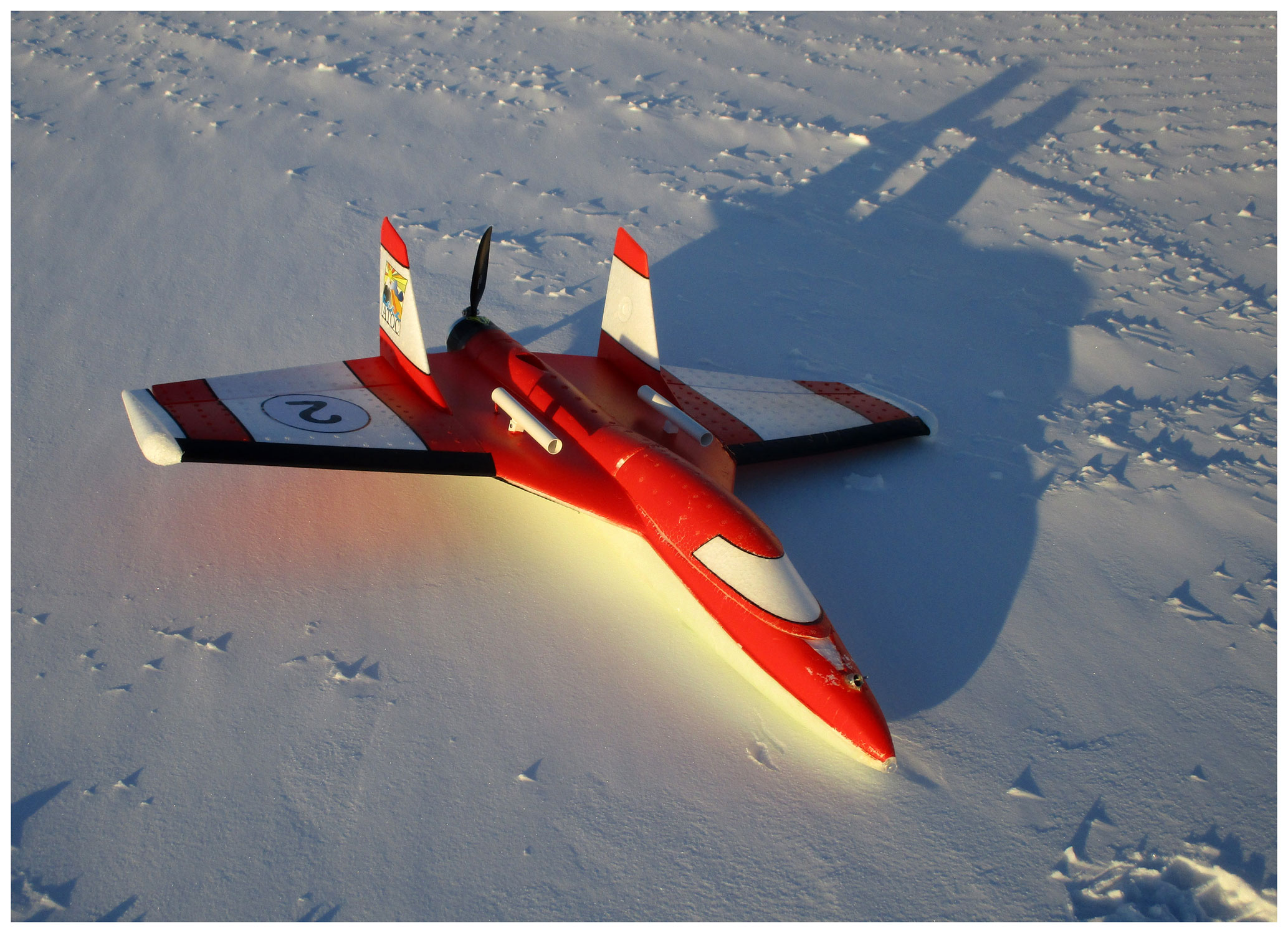
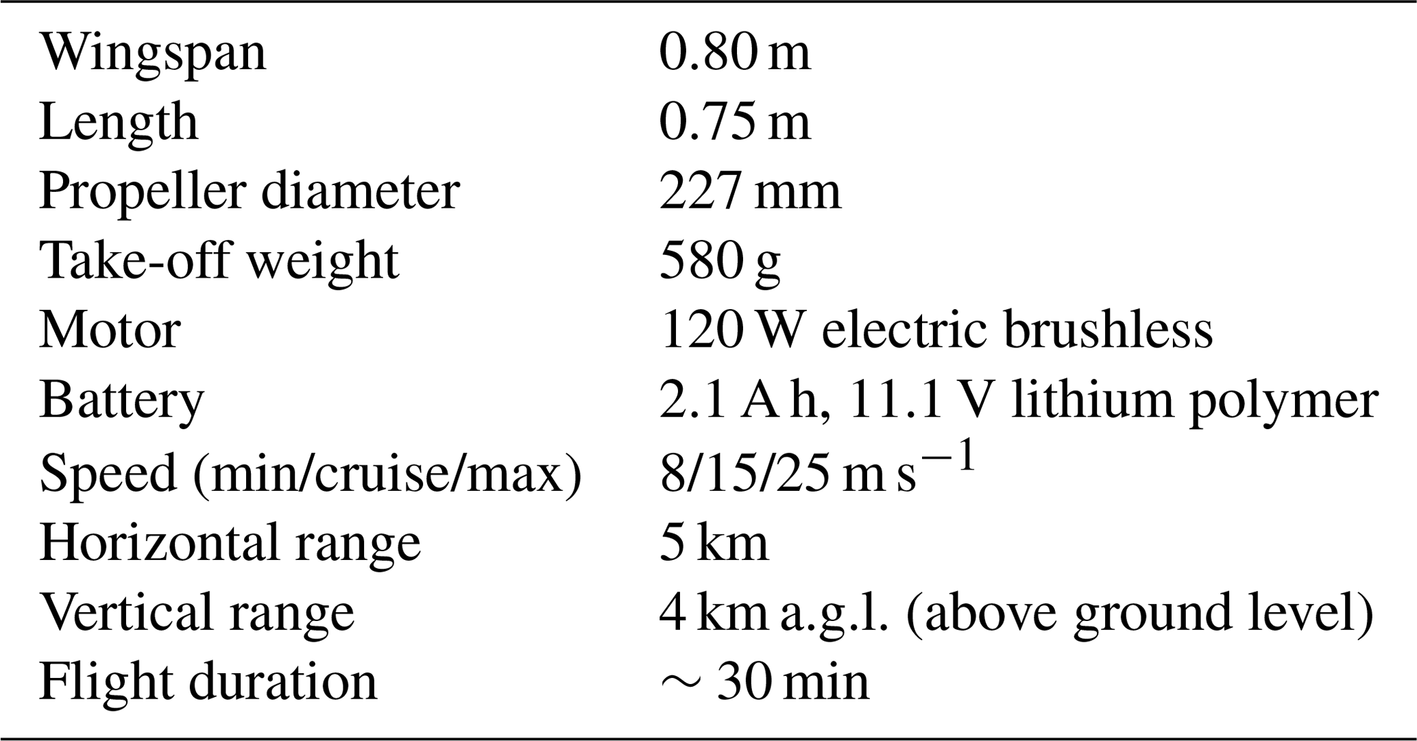
Reuder et al. (2009, 2012), Cassano (2014), and Jonassen et al. (2015) provide technical descriptions of the SUMO sUAS. The SUMO is a small fixed-wing pusher prop drone with 0.80 m wingspan and 580 g take-off weight that is constructed from high-density foam (Fig. 2). The airframe is based on the commercially available Multiplex FunJET model remote control airplane. The SUMO uses a single lithium polymer (LiPo) battery to power the electric motor, which allows for a flight time of ∼30 min. Further details about the SUMO sUAS are given in Table 1.

Table 1 SUMO sUAS airframe and flight specifications (based on Reuder et al., 2012; Cassano, 2014).

The SUMO sUAS is launched by hand and lands on its underside. Usually a two-person team operates the SUMO. One person, the remote control pilot, maintains visual sight of the aircraft and controls the SUMO via a remote control, while the second flight team member, the ground station pilot, manages the ground control software. A standard model airplane remote control can be used to manually control the SUMO sUAS, but it is typically flown in a semiautonomous or autonomous mode via the onboard Paparazzi autopilot (ENAC, 2008) and ground control software (Table 2). A 2.4 GHz radio modem is used for two-way communication between the SUMO and the ground control software. The SUMO observations are relayed to the ground station computer, and the preprogrammed flight plan can be modified with the ground station software via the radio modem link. In the case of a ground station communication failure, the remote control pilot can take control of the aircraft at any time.

Table 2 SUMO sUAS navigation, control and communication and scientific instrumentation sensor range, accuracy, acquisition frequency and time constant, as specified by the manufacturer (based on Reuder et al., 2012; Cassano, 2014).

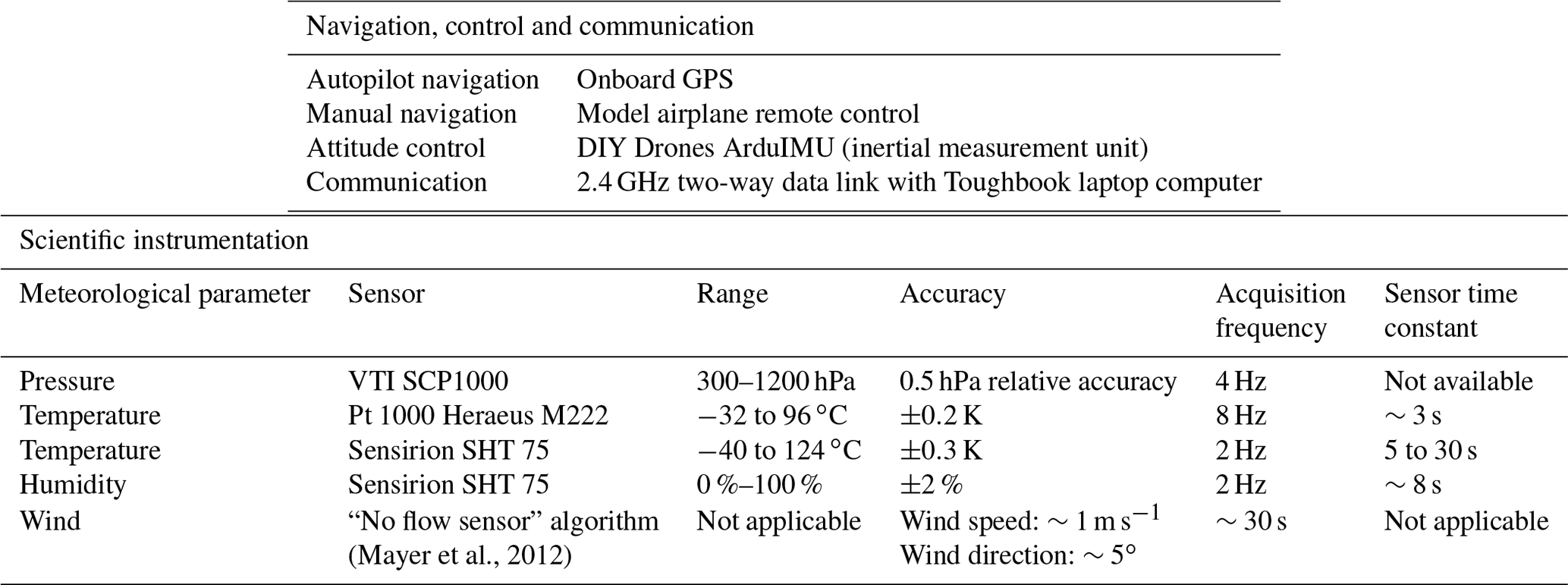
The SUMO records temperature, humidity, pressure and aircraft location at 2 to 8 Hz frequency (Table 2). Temperature is measured with a reported accuracy of ±0.2 K (±0.3 K) for the Pt 1000 (Sensirion) sensor. The temperature sensor specifications indicate a time lag of 3 to 30 s, but a comparison between the two temperature sensors indicate that both have a similar lag of 2 to 5 s. The sensor lag appears as an offset between ascending and descending temperature profiles during flights with continuous spiral ascent and descent flight patterns as shown in Cassano (2014) and discussed in Sect. 4. As a result of this sensor lag, most of the SUMO flights described in this paper used stepped ascent or descent profiles (described in more detail below). Each step in these ascent/descent patterns occurred over roughly 65 s, so the temperature sensor lag becomes unimportant as it is much shorter than the orbit time at each height. The reported sensor time constant for relative humidity measurements, made with the Sensirion SHT 75 sensor, is approximately 8 s, although at temperatures well below 0 ^∘C, we found that the humidity data were largely unusable due to very long time lags. The Mayer et al. (2012) “no flow sensor” method was used to estimate wind speed and direction by evaluating differences in ground speed throughout a circular flight path and is described in greater detail in Sect. 3.

2.2 Flight strategy

A total of 116 SUMO sUAS flights took place between January 2012 and June 2017 at several locations in Antarctica (Fig. 1). Many of these flights took place over permanent ice shelf locations with 8 flights at Williams Field, 39 flights at the Pegasus ice runway and 36 flights at the Tall Tower automatic weather station (AWS) site (Wille et al., 2017). Pegasus runway and Williams Field are within 20 km of the main United States Antarctic Program research base, McMurdo Station, and Ross Island, which has a maximum elevation in excess of 4000 m. The Tall Tower AWS flights took place approximately 160 km south-southeast of McMurdo Station in a region of almost completely flat permanent ice with no major topographic features within 85 km of the site. Other continental flights occurred near Lake Vanda in the ice-free McMurdo Dry Valleys (14 flights). Finally, several flights occurred over sea ice in the western Ross Sea as part of the PIPERS cruise (19 flights; Ackley et al., 2020). To avoid issues related with aircraft icing, all flights occurred in cloud-free conditions over the altitude range of the flight, although clouds above the maximum flight level were present for some flights. Table A1 lists the date and time, location, and maximum altitude for each flight.

Additional Antarctic SUMO flights had been planned to take place after the PIPERS cruise in 2017, but challenges in attempting to schedule a midwinter campaign, as well as the recent Antarctic field work restrictions due to COVID-19, resulted in the 2017 flights being the last SUMO flights conducted in Antarctica. As such, this paper provides a description of all Antarctic SUMO UAS flights that have been, or will be, conducted by our research group. Future sUAS flights in Antarctica led by our group will use the DataHawk2 sUAS developed at the University of Colorado – Boulder (Lawrence and Balsley, 2013).

The primary scientific objective for all of our Antarctic SUMO flights was to obtain profiles of the atmospheric state of the boundary layer. During a given flight day, SUMO boundary layer profile flights would occur every hour to several hours, although other factors, including weather and logistics, could limit the frequency and number of flights that could be performed. Changes in the atmospheric thermodynamic state between pairs of SUMO profile flights allowed for the estimation of the surface turbulent fluxes based on state changes within the boundary (Bonin et al., 2013; Båserud et al., 2020), as well as estimates of large-scale advective changes based on state changes above the boundary layer. The relatively high temporal resolution atmospheric profiles observed by the SUMO were also used to assess the Antarctic Mesoscale Prediction System (Powers et al., 2012) operational weather forecasts (Wille et al., 2017).

A typical flight started with the SUMO manually or semiautonomously controlled by the remote control pilot. Immediately after launch, the remote control pilot would ensure that the SUMO sUAS was performing as expected and would then switch the aircraft to the fully autonomous flight mode. The aircraft would then climb to a specified height (usually 50 m a.g.l., above ground level) and orbit until instructed by the ground control pilot via the ground control software to begin the profiling portion of the flight. A stepped spiral ascent/descent flight pattern was usually used, with the aircraft set to orbit at several different heights below a maximum altitude of 1000 m a.g.l. For most flights, a stepped ascent was followed by a continuous descent, although some flights had a stepped ascent, followed by a stepped descent. A few flights were also flown with a continuous spiral ascent, followed by a continuous spiral descent, although as discussed above this flight pattern resulted in noticeable artifacts due to sensor lag. For both the stepped and continuous profiles the spiral diameter was approximately 250 m. The SUMO would complete two circular orbits in approximately 65 s at each specified height in the stepped ascent/descent profile before climbing or descending to the next fixed-height orbit location. Once the profiling was completed the aircraft would return to a height of approximately 50 m and orbit until the remote control pilot took control of the aircraft to land it in either manual or semiautonomous mode.

The boundary layer depth in the Antarctic can vary from tens of meters or less during strongly stable, light wind conditions in winter to more than 1000 m in summer (King and Turner, 1997). The maximum SUMO spiral profile heights ranged from 89 to 1371 m a.g.l. (Table A1) and sampled the full depth of the boundary layer for all but a few flights. The continuous spiral ascent and descent flight pattern, up to 1000 m a.g.l., usually took about 10 min to complete, and two to three profiles could be completed in a single flight. For the stepped ascent or descent profile flight patterns, it was usually possible to complete 18 fixed-height orbits during a 30 min flight.

3 Data processing and quality control

Data from the SUMO sUAS were logged using an onboard data logger controlled through the Paparazzi autopilot software. These data were telemetered via 2.4 GHz radio modem to a laptop computer running the Paparazzi ground control software and also logged to an onboard SD memory card. The data in the telemetered and SD data streams were identical other than a reduced temporal resolution and occasional gaps in the record in the telemetered data. The SD data stream was used as the source data for the archived data except for cases when the SD data were not available due to memory card failure or other issues.

The data recorded by the SUMO, in both the telemetered and SD data stream, are written sequentially with each record marked with the elapsed time since the SUMO was powered on. Each data record reported a single variable – aircraft status, navigation information or data from one of the scientific instruments. These data were stored in text log files on the ground station computer and the onboard SD card.

Following each flight, the SUMO SD or telemetered log files were processed into a comma-separated text file. A header was written to this file that listed the flight location, sUAS pilots, and start date and time of the flight. Each subsequent line of the file listed the date and time, elapsed time since SUMO power on, location, and meteorological data (Table A2) at the same temporal frequency as the original SUMO data file. The date and time variables were calculated from the date and time on the ground station laptop when the SUMO was powered on and the elapsed time reported for each record in the data file. Since each time period reported in the SUMO data file listed a single variable, all other variables were flagged as missing values (–9999) for that time period. These data files were named yy_mm_dd__HH_MM_SS_SD.txt, where yy is year, mm is month, dd is day, HH is hour, MM is minute, and SS is second of the SUMO power on time in coordinated universal time (UTC). The _SD indicates that the data are from an SD file. If the data came from a telemetered SUMO log file, the _SD was omitted in the filename.

A second data processing step linearly interpolated all variables in time to replace the missing data values and provide data for all variables at each time step in the data file. No interpolation was performed before a given variable was first reported in the log file, so these records retain missing data values. These data were written to files with the same naming convention as above but with _ interpolation added to the filename before the .txt filename extension to indicate the temporal interpolation was applied to the original data.

The interpolated data were then used to calculate averages from each constant altitude orbit completed during the flight and vertical bin averages. As described above, most SUMO flights were conducted such that the sUAS orbited at multiple fixed heights over the flight altitude range. These fixed-height orbits helped address sensor time lag issues and also allowed the Mayer et al. (2012) “no flow sensor” algorithm to estimate winds at a constant altitude. This processing step identified flight segments that remain within ±8 m of all other points in the segment and for all segments when the SUMO's position on the circular orbit passed through a full 360^∘ (i.e., one complete circular orbit). For each flight segment identified in this way, the wind speed and direction were estimated following Mayer et al. (2012), and the average altitude, temperature, relative humidity and pressure were calculated. The wind speed was estimated based on the difference between the minimum and maximum GPS ground speed recorded during the circular orbit. The wind direction was calculated based on the orbit heading at the location of the minimum and maximum GPS speed, with both directions reported in the archived data file. The start and end time, heading, and altitude, as well as elapsed time, on the constant height orbit were also reported in the archived data file named yy_mm_dd__HH_MM_SS_SD_const_alt.txt. All data stored in the constant altitude archived data file are listed in Table A2.

Vertical bin averages were calculated for each 5 m altitude bin over the full altitude range of each SUMO flight. For each vertical altitude bin, the average, standard deviation and number of observations in the bin were calculated. These values were calculated from all data during the flight, as well as from data from the ascent-only and descent-only portions of the flight. There data are stored in files named yy_mm_dd__HH_MM_SS_SD_vert_avg.txt (Table A2).

Data from each flight in the interpolated data file, as well as from the vertical bin average and constant altitude orbit data files, were visually inspected. The following issues were observed, but no data were removed from the archived data files. For each flight, there is a short period, of a few seconds, when the temperature sensors adjust to the ambient conditions immediately after take-off. As noted in Sect. 2.1, there is a noticeable sensor lag evident in the temperature and humidity measurements. The sensor lag is short, of the order of a few seconds, for the temperature measurements but is much longer for the humidity observations. These lags are obvious when comparing observations from the ascent and descent portions of the flight (Fig. 3). Since the original time resolution data are provided, users of these data can apply whatever corrections are needed for their application to account for the sensor lag, but no corrections were applied to the archived data.

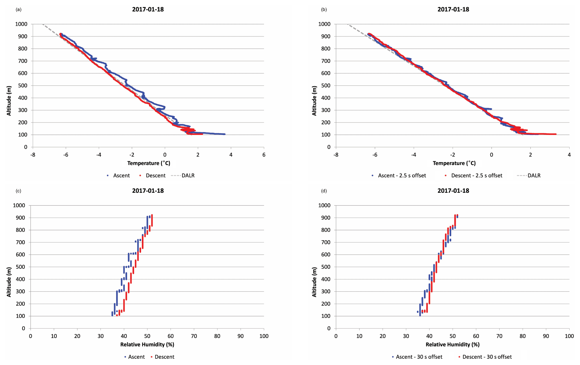
Figure 3 Temperature (a, b) and relative humidity (c, d) profiles observed by the SUMO sUAS in the Wright Valley, Antarctica, at 02:01 UTC, 18 January 2017. The original time interpolated data are plotted in panels (a) and (c), and data with a time lag of 2.5 and 30 s are plotted in panels (b) and (d), respectively. In panels (a) and (b), the dry adiabatic lapse rate (DALR) is shown with a dashed gray line.

Figure 3 illustrates the sensor lag for temperature and humidity measurements for a SUMO flight conducted at 02:01 UTC, 18 January 2017, in the Wright Valley. During this flight, a deep, convective boundary layer was present. Figure 3a shows the temperature observed during the stepped ascent (blue) and spiral descent (red) portions of this flight. The ascent portion of the flight is consistently warmer than the descent and, given the decreasing temperature with height on this day, is consistent with a short time lag in the temperature measured by the SHT sensor. By applying a 2.5 s offset to the temperature relative to the height, the ascent and descent profiles more closely match (Fig. 3b). This time lag is consistent with results presented by Cassano (2014). The humidity observations also exhibit a time lag (Fig. 3c). Here, humidity increases with height, and the time lag results in the ascending observations being shifted to slightly lower relative humidity values at a given height compared to the observations during the descent. While the manufacturer-stated sensor time constant for the humidity sensor is ∼8 s, we have found that applying a 30 s time shift to the humidity measurements results in a much closer correspondence between the humidity profiles observed during the SUMO ascent and descent (Fig. 3d), although this does not fully remove the discrepancies between the ascent and descent profiles as seen for temperature (Fig. 3b). The longer time constant for the humidity measurements presented here, compared to the manufacturer's specification, may be caused by a lower ambient temperature during these flights than used by the manufacturer.

4 Examples of observed features

With SUMO flights being conducted throughout the full annual cycle and over a variety of surface conditions across the Antarctic continent, a wide range of boundary layer stability, depth and evolution has been observed. Some examples of the variety of boundary layer states observed by the SUMO sUAS are given below.

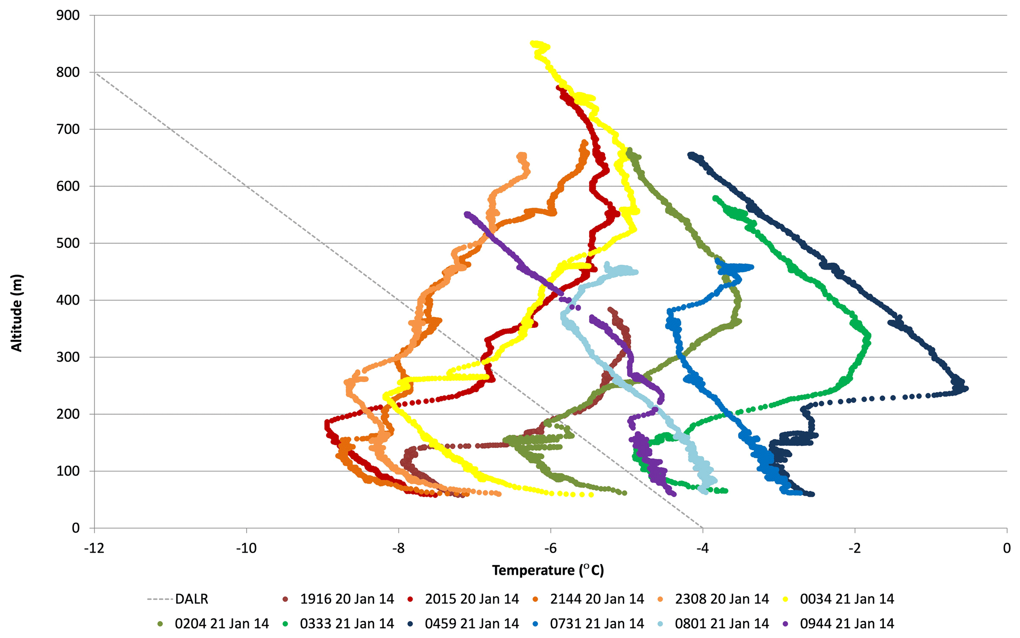
Figure 4 SUMO observed temperature profiles (plotted as colored lines) at the Ross Ice Shelf Tall Tower AWS site from 19:16 UTC, 20 January 2014, to 09:44 UTC, 21 January 2014. The dry adiabatic lapse rate (DALR) is shown with a dashed gray line.

A total of 11 SUMO flights were conducted at the Ross Ice Shelf Tall Tower site over a 14.5 h period from 19:16 UTC, 20 January 2014, to 09:44 UTC, 21 January 2014 (Fig. 4). The timing between most of these flights was ∼1.5 h, which provided a detailed depiction of the temporal evolution of the boundary layer and free atmosphere above.

From 19:16 UTC, 20 January, to 02:04 UTC, 21 January, a shallow, well-mixed boundary was observed with a dry adiabatic temperature profile up to a maximum height of 250 m. After 02:04 UTC, the boundary layer transitioned to a weakly stable temperature profile. The temperature in the boundary layer initially cooled (19:16 to 21:44 UTC, 20 January) by ∼1 K and then warmed by ∼5 K by 07:31 UTC, 21 January, before cooling by ∼2 K over the next approximately 2 h.

The temperature above the boundary layer was not constant during the 14.5 h sampling period from 20–21 January 2014. Here, we assume that the temperature change observed above the boundary layer is due to large-scale advective changes, but other processes such as adiabatic changes due to vertical motion or radiative heating or cooling may also contribute to the observed temperature trends. Further analysis would be required to determine the relative role of each of these processes in altering the temperature aloft. Considering the temperature at 300 m, it cooled by ∼3 K from 19:16 to 23:08 UTC, 20 January. This cooling was greater than what was observed in the boundary layer during this same time period and suggests that large-scale advective cooling, as inferred from the cooling aloft, was offset by an upward sensible heat flux in the boundary layer, which is consistent with the convective conditions observed at this time. Over the next four flights (00:34 to 04:59 UTC, 21 January), the temperature at 300 m warmed by almost 8 K, while the boundary layer temperature did not warm as much. This suggests that large-scale warm advection occurring at this time was offset by either radiative cooling or a downward sensible heat flux in the boundary layer, which is consistent with the transition from a convective to slightly stable boundary layer during this time period. During the final three flights (07:31 to 09:44 UTC, 21 January), cooling of ∼1 K was observed aloft and in the boundary layer.

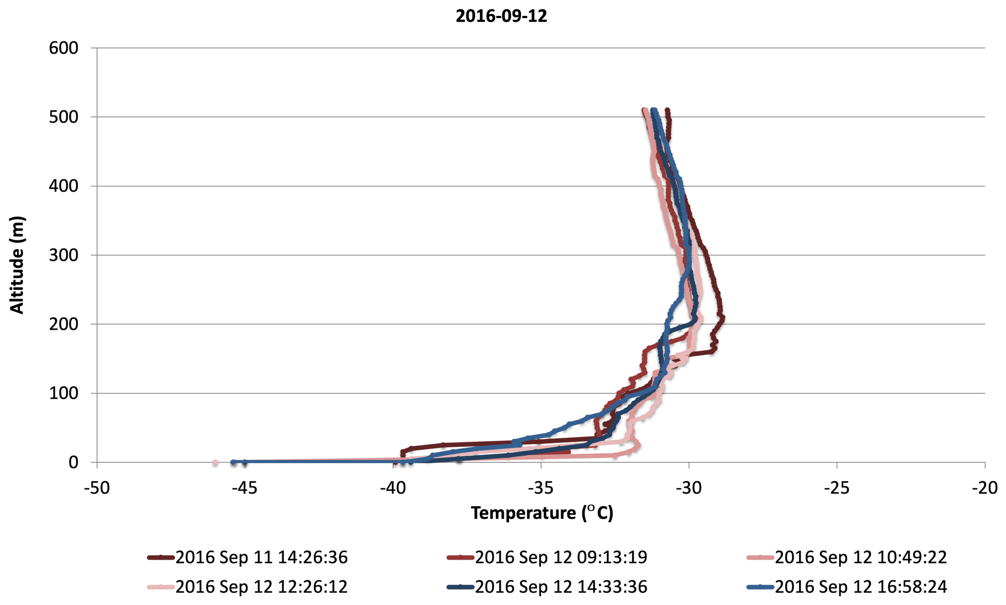
Figure 5 SUMO observed temperature profiles (colored lines) at the Pegasus ice runway from 14:26 UTC, 11 September 2016, to 16:58 UTC, 12 September 2016.

Contrasting the summer conditions seen in Fig. 4, Fig. 5 shows temperature profiles observed during 11–12 September 2016 at the Pegasus runway at the end of the Antarctic winter. Six SUMO flights were completed between 14:26 UTC, 11 September, and 16:58 UTC, 12 September 2016. The surface temperature during these flights was near −40 ^∘C, which is the lower observation limit of the SHT temperature sensor. Unlike the temperature profiles shown in Fig. 4, the temperature profiles observed during the 24 h plus period from 11 to 12 September 2016 (Fig. 5) showed a remarkable lack of temporal variability, exhibiting nearly steady-state conditions. During this time, a very strong, shallow surface inversion was present with the temperature warming by ∼7 K in the lowest 50 m of the sounding and then warming by another several kelvin up to 200 m.

Figure 6 SUMO observed temperature profiles (colored lines) near Lake Vanda in the Wright Valley from 17:00 UTC, 16 January 2017, to 02:01 UTC, 18 January 2017. The dry adiabatic lapse rate (DALR) is shown with a dashed gray line.

During the austral summer of 2017, SUMO flights were conducted in the Wright Valley, near Lake Vanda, at one of the few permanently ice-free locations on the Antarctic continent. The temperature profiles observed from 16 to 18 January 2017 (Fig. 6) differ markedly from the profiles shown in Figs. 4 and 5. The boundary layer observed in the Wright Valley was a deep convective boundary layer with a surface temperature near or just above 0 ^∘C. From late morning to midafternoon local time (19:33 UTC, 17 January 2017, to 02:01 UTC, 18 January 2017), the boundary layer warmed by ∼2 K and deepened from 200 m to more than 800 m, with a dry adiabatic lapse rate (DALR) extending beyond the top flight altitude of the SUMO at 00:57 and 02:01 UTC, 18 January 2017.

5 Code availability

All code used to process the SUMO data is available by request to the corresponding author.

6 Data availability

The SUMO sUAS data described in this paper can be retrieved from the United States Antarctic Program Data Center (https://www.usap-dc.org, last access: 8 March 2021). The data for all flights conducted on the continent (Williams Field, Pegasus runway, Tall Tower AWS site and Wright Valley) are available at https://doi.org/10.15784/601054 (Cassano, 2017), and data from the PIPERS cruise, in the Ross Sea, are available at https://doi.org/10.15784/601191 (Cassano, 2019). The data are archived in annual zip files that contain comma delimited text files of the data at their original and interpolated time resolution and as vertical bin-averaged and constant altitude data. Each data file contains a header that lists the flight location name, latitude, longitude, start date and time (UTC) of the flight, and the sUAS pilots. A final header line lists the data type and units contained in each comma-separated column in the remainder of the file.

7 Summary

Between January 2012 and June 2017, a small unmanned aerial system (sUAS), known as the Small Unmanned Meteorological Observer (SUMO), was used to observe the temperature, humidity, pressure and wind in and above the Antarctic atmospheric boundary layer. During six Antarctic field campaigns, 116 SUMO flights were completed. Flights over ice shelf locations occurred at Williams Field and the Pegasus runway (two field campaigns), both located within 20 km of McMurdo Station and Ross Island, and at the Tall Tower AWS site located in the northwestern portion of the Ross Ice Shelf (Fig. 1). Flights also took place in the ice-free Wright Valley near Lake Vanda in a region of complex terrain and were performed over sea ice in the western Ross Sea as part of the PIPERS research cruise (Ackley et al., 2020). These flights took place during all seasons with most of the flights conducted during the austral summer (January) and late winter/early spring (September). The flights observed the full depth of the atmospheric boundary layer and a portion of the free atmosphere above, with the SUMO flying a spiral ascent and descent flight path. A wide variety of boundary layer states were observed, including very shallow, strongly stable conditions during the Antarctic winter (Fig. 5) and deep, convective conditions over ice-free locations in the summer (Fig. 6).

Data from these flights were processed from the native SUMO log files into comma-separated text files at the original and an interpolated time resolution. Additional data processing of the interpolated time resolution data created vertical bin-averaged data and averages over constant altitude SUMO orbits. Errors noted in the data include short periods of time at the start of the flight when the meteorological sensors equilibrate with the ambient atmospheric conditions and time lags in the temperature (∼2.5 s) and humidity (30 s or more) measurements.

The Antarctic atmospheric boundary layer data collected by the SUMO sUAS, described in this paper, are freely available from the United States Antarctic Program Data Center (https://www.usap-dc.org). The data for all flights conducted on the continent (Williams Field, Pegasus ice runway, Tall Tower AWS site and Wright Valley) are available at https://doi.org/10.15784/601054 (Cassano, 2017), and data from the PIPERS cruise Ross Sea flights are available at https://doi.org/10.15784/601191 (Cassano, 2019).

Appendix A

Table A1 UTC date and time (yymmdd_HHMM format; yy: year; mm: month; dd: day; HH: hour; MM: minute), location, flight duration (s), maximum altitude above ground level (a.g.l.) and profile type (SA: stepped ascent; CA: continuous ascent; SD: stepped descent; CD: continuous descent) for all SUMO flights.

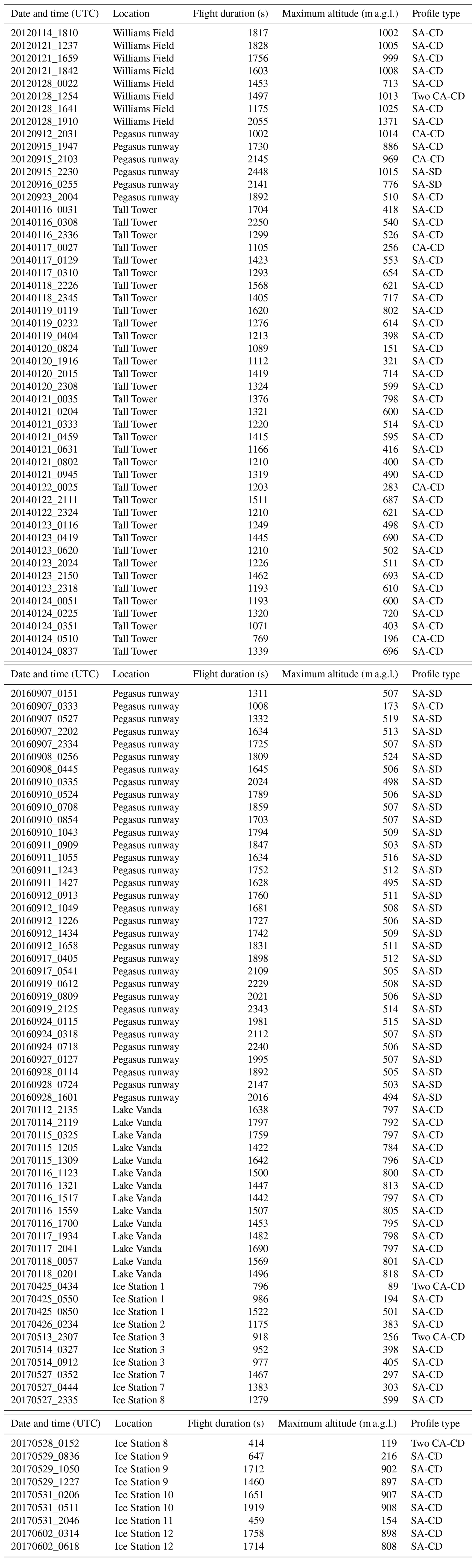
Table A2 Post-processed SUMO data files and data archived in each type of post-processed file.

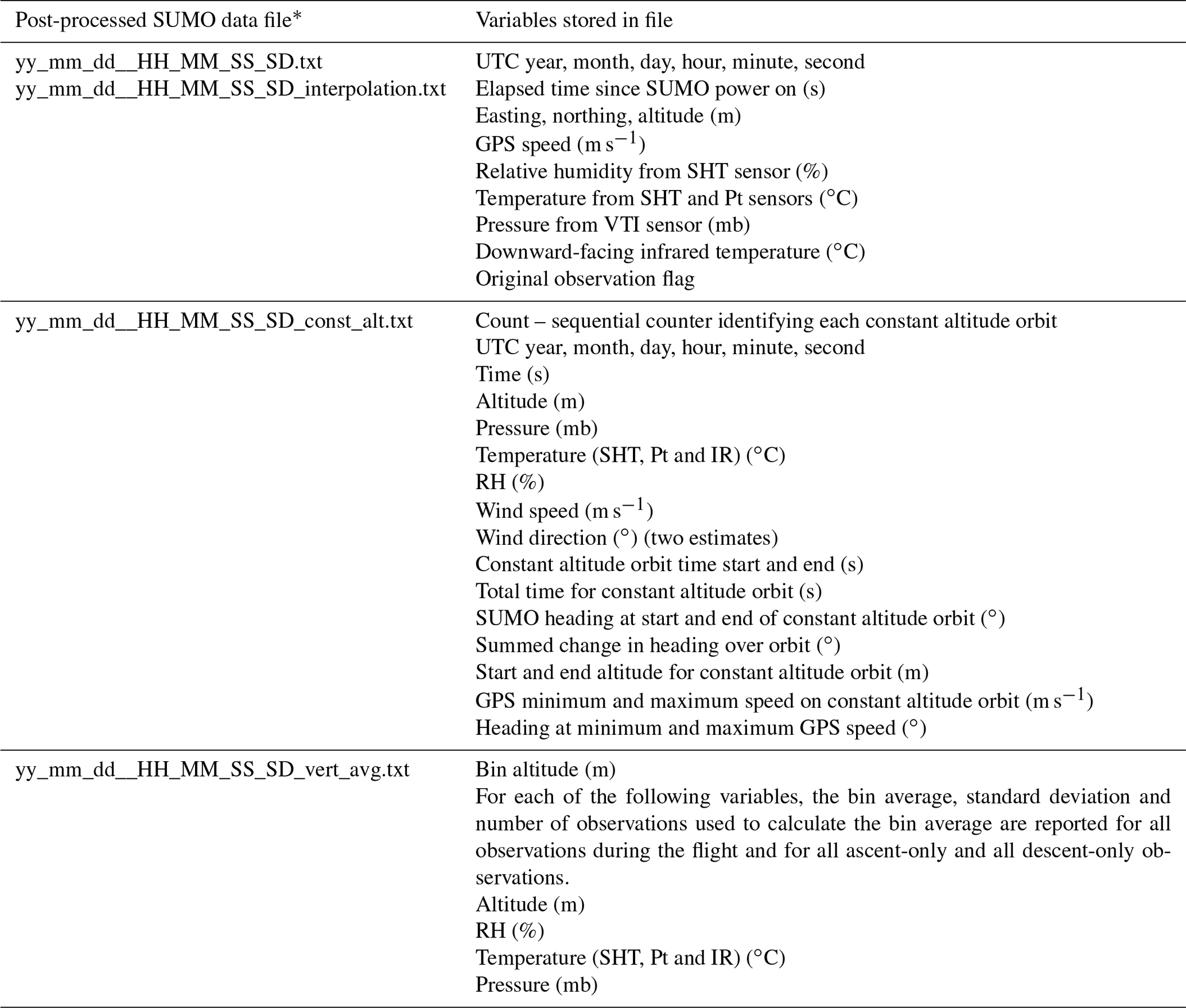
* _ SD portion of filename is omitted if data came from telemetry data stream rather than SD data stream.