the Creative Commons Attribution 4.0 License.
the Creative Commons Attribution 4.0 License.
 | 03 Mar 2021
A high-resolution unified observational data product of mesoscale convective systems and isolated deep convection in the United States for 2004–2017
Yun Qian
L. Ruby Leung
Deep convection possesses markedly distinct properties at different spatiotemporal scales. We present an original high-resolution (4 km, hourly) unified data product of mesoscale convective systems (MCSs) and isolated deep convection (IDC) in the United States east of the Rocky Mountains and examine their climatological characteristics from 2004 to 2017. The data product is produced by applying an updated Flexible Object Tracker algorithm to hourly satellite brightness temperature, radar reflectivity, and precipitation datasets. Analysis of the data product shows that MCSs are much larger and longer-lasting than IDC, but IDC occurs about 100 times more frequently than MCSs, with a mean convective intensity comparable to that of MCSs. Hence both MCS and IDC are essential contributors to precipitation east of the Rocky Mountains, although their precipitation shows significantly different spatiotemporal characteristics. IDC precipitation concentrates in summer in the Southeast with a peak in the late afternoon, while MCS precipitation is significant in all seasons, especially for spring and summer in the Great Plains. The spatial distribution of MCS precipitation amounts varies by season, while diurnally, MCS precipitation generally peaks during nighttime except in the Southeast. Potential uncertainties and limitations of the data product are also discussed. The data product is useful for investigating the atmospheric environments and physical processes associated with different types of convective systems; quantifying the impacts of convection on hydrology, atmospheric chemistry, and severe weather events; and evaluating and improving the representation of convective processes in weather and climate models. The data product is available at https://doi.org/10.25584/1632005 (Li et al., 2020).
- Article
(33313 KB) - Full-text XML
- BibTeX
- EndNote


In the atmosphere, deep convection refers to thermally driven turbulent mixing that displaces air parcels from the lower atmosphere to the troposphere above 500 hPa (Davison, 1999), leading to the development of convective storms. The heavy rain rates associated with deep convection can significantly affect the water cycle (Hu et al., 2020) and other aspects such as soil erosion (Nearing et al., 2004), surface water quality (Carpenter et al., 2018; Motew et al., 2018), and managed and unmanaged ecosystems (Angel et al., 2005; Derbile and Kasei, 2012; Rosenzweig et al., 2002) that are essential elements of the biogeochemical cycle. By redistributing heat, mass, and momentum within the atmosphere, deep convection also has important effects on atmospheric chemistry (Anderson et al., 2017; Andreae et al., 2001; Choi et al., 2014; Grewe, 2007; Thompson et al., 1997; Twohy et al., 2002), large-scale environments (Houze Jr, 2004; Piani et al., 2000; Stensrud, 1996, 2013; Wang, 2003), and radiation balance (Feng et al., 2011; Zhang et al., 2017).
Besides its effects on the energy, water, and biogeochemical cycles, deep convection also has more direct societal impacts. As a significant source of natural hazards such as tornadoes, hail, wind gusts, lightning, and flash flooding, deep convection poses critical threats to human life and property (Brooks et al., 2003; Doswell et al., 1996; Koehler, 2020; Taszarek et al., 2020). During 1950–1994, deep convection thunderstorms produced 47 % of annual rainfall and up to 72 % of summer rainfall on average east of the Rocky Mountains (Changnon, 2001b). During the same period, both the number of severe thunderstorms and amount of deep convection precipitation have increased in most regions of the contiguous United States (CONUS) (Changnon, 2001a, b; Groisman et al., 2004). Folger and Reed (2013) found that hazards associated with thunderstorms have accounted for 57 % of annual insured catastrophe losses since 1953. Since the 1980s, the inflation-adjusted economic losses due to convective storms have increased from about USD 5 billion to about USD 20 billion in recent decade (https://www.iii.org/fact-statistic/facts-statistics-tornadoes-and-thunderstorms, last access: 30 March 2020). With warmer temperatures, the environments of hazardous convective weather are projected to become more frequent in the future (Diffenbaugh et al., 2013; Seeley and Romps, 2015), although few robust trends have emerged in the recent decades (Houze Jr et al., 2019; Tippett et al., 2015).
The crucial roles of deep convection motivate the need for more accurate and comprehensive datasets to improve understanding and modeling of this process and its impacts. To this end, datasets with information on the location and time of occurrence, intensity, and other properties of deep convection are necessary to understand and quantify its impacts on the hydrologic cycle, severe weather hazards, large-scale circulations, etc. While field campaign data can provide detailed information on deep convection properties, they are limited in space-time coverage for statistical analysis. A corresponding reliable long-term dataset is undoubtedly useful for model evaluation and development (Prein et al., 2017; Yang et al., 2017).
Deep convection can exist as isolated convective storms or organized storms with mesoscale structures. A mesoscale convective system (MCS) is an aggregate of convective storms organized into a larger and longer-lived system, which is the largest type of deep convection. Due to their much longer duration and broader spatial coverage, MCSs generally have stronger and longer-lasting influences on large-scale circulations than isolated deep convection (IDC) events (Bigelbach et al., 2014; Stensrud, 1996, 2013). MCSs may also produce higher rain rates, larger echo top heights, and greater water and ice masses than IDC (Rowe et al., 2011, 2012). The enhanced rain rates in MCSs might be caused by larger amounts of ice falling out and melting, higher amounts of liquid water below the melting level, and higher concentrations of smaller drops (Rowe et al., 2011, 2012). Rowe et al. (2012) also suggested that the enhanced rainfall from MCSs might be associated with more favorable environmental conditions, such as higher convective available potential energy (CAPE) and wind shear. CAPE and wind shear can impose different impacts on the initiation and evolution of IDC and MCSs (French and Parker, 2008).
Considering the significant differences between IDC and MCS events, a reliable long-term dataset not only describing the characteristics of deep convection but also separating IDC events from MCSs is useful. With the deployment of operational remote sensing platforms such as geostationary satellites and ground-based radar network several decades ago, scientists have developed numerical algorithms to automatically detect deep convective systems and track their evolutions over large areas and for long durations on the basis of continuous measurements from remote sensors (Cintineo et al., 2013; Feng et al., 2011; Feng et al., 2012; Futyan and Del Genio, 2007; Geerts, 1998; Hodges and Thorncroft, 1997; Liu et al., 2007; Machado et al., 1998). Objective tracking of deep convection has been applied to geostationary satellite data (Cintineo et al., 2013; Sieglaff et al., 2013; Walker et al., 2012) and Next Generation Weather Radar (NEXRAD) data (Haberlie and Ashley, 2019; Pinto et al., 2015) in the United States (US) over different periods. However, a long-term climatological data product of MCS and IDC events over the CONUS has heretofore not been developed.
Here, building on the work by Feng et al. (2019), which developed an algorithm for MCS tracking and a dataset for MCSs for the eastern CONUS, we produce a unified high-resolution data product of both MCS and IDC events and analyze their characteristics east of the Rocky Mountains for 2004–2017. The data product is developed by applying an updated Flexible Object Tracker (FLEXTRKR) algorithm (Feng et al., 2018, 2019) and the Storm Labeling in Three Dimensions (SL3D) algorithm (Starzec et al., 2017) to the NCEP (National Centers for Environmental Prediction)/CPP (the Climate Prediction Center) L3 4 km Global Merged IR V1 brightness temperature (Tb) dataset (Janowiak et al., 2017), the 3-D Gridded NEXRAD Radar (GridRad) dataset (Homeyer and Bowman, 2017), the NCEP Stage IV precipitation dataset (Lin and Mitchell, 2005), and melting level heights from ERA5 (ECMWF, 2018). Section 2 describes the updated FLEXTRKR and SL3D algorithms in detail, as well as the source datasets used by the algorithms. In Sect. 3, we first compare the climatological characteristics between MCS and IDC events based on the MCS–IDC data product. Then, as an application of the data product, we examine the spatiotemporal precipitation characteristics of MCS and IDC events. In Sect. 4, we discuss the uncertainties and limitations of the data product. Section 5 provides the availability information of the data product. Finally, we summarize the study in Sect. 6.
2.1 Source datasets
2.1.1 Merged 4 km infrared brightness temperature dataset
In this study, we identify cold clouds associated with MCSs and IDC by using the NOAA NCEP/CPP L3 half-hourly 4 km Global Merged IR V1 infrared Tb data for 2004–2017 (Janowiak et al., 2017). The dataset is a combination of various geostationary IR satellites with parallax correction and viewing angle correction, therefore providing continuous coverage globally from 60∘ S–60∘ N with a horizontal resolution of about 4 km and a temporal resolution of 0.5 h (Janowiak et al., 2001). We only use the hourly Tb data in the FLEXTRKR algorithm discussed below, as all other datasets are only available at an hourly interval.
2.1.2 Three-dimensional Gridded NEXRAD Radar (GridRad) dataset
GridRad is an hourly 3-D radar reflectivity (ZH) mosaic combining individual NEXRAD radar observations to a Cartesian gridded dataset, with a horizontal resolution of 0.02∘ × 0.02∘ and a vertical resolution of 1 km. The dataset covers 115 to 69∘ W in longitude, 25 to 49∘ N in latitude, and 1 to 24 km in altitude above sea level (a.s.l.). Homeyer and Bowman (2017) produced the dataset by applying a four-dimensional binning procedure to merge level-2 ZH data from 125 National Weather Service (NWS) NEXRAD weather radars to GridRad grid boxes at analysis times. Only the level-2 observations within 300 km of each radar and 3.8 min of the analysis time were used in the binning procedure. The GridRad ZH was the weighted average of the level-2 observations within the GridRad grid boxes to reduce the potential loss of information. The weight calculation of each level-2 observation followed a Gaussian scheme in both space and time. Observation weight was negatively correlated with the distance of the observation from the source radar and the time difference between the observation and analysis time. The GridRad dataset provides the total weight of the level-2 observations within each GridRad grid box, which is useful for quality control. In addition, the number of level-2 radar observations (Nobs) and the number of level-2 radar observations with echoes (Necho) within each GridRad grid box around analysis times (±3.8 min) are also available in the GridRad dataset.
We obtain the GridRad datasets between 2004 and 2017 from NCAR/UCAR Research Data Archive (RDA) (https://rda.ucar.edu/datasets/ds841.0/, last access: 2 January 2020). Following the quality control criteria of Homeyer and Bowman (2017) (http://gridrad.org/software.html, last access: 22 January 2020), we remove potential low-quality observations, scanning artifacts, and non-meteorological echoes from biological scatters and artifacts. Then we regrid GridRad ZH onto the 4 km satellite Merged IR grids by using the “bilinear” method from the Earth System Modeling Framework (ESMF) Python module (https://www.earthsystemcog.org/projects/esmpy/, last access: 14 February 2020) as follows.
First, we convert the GridRad logarithmic reflectivity ZH to linear reflectivity (Z′: mm6 m−3). We then set Z′ in grid boxes with radar observations but no echoes (Nobs>0, but ZH= NAN; NAN, Not a Number) to 0 (). Here the physical interpretation is that NEXRAD scans those grid boxes, but no detectable hydrometeors return any echo. The primary motivation of this procedure is to avoid the reduction of the number of valid reflectivity values after re-gridding, as the ESMF bilinear method treats the destination point as a NAN as long as there is one NAN value in the source points. A common scenario is at the edge between hydrometeor echoes and clear air. Setting Z′ of those grid boxes having radar observations but no echoes to NAN would cause all surrounding destination points to become NAN even though all other source points have valid Z′ values, which would reduce the number of re-gridded valid ZH (ZH≠ NAN) values by about 20 % for 2004–2017. After the “bilinear” re-gridding of Z′, we convert the linear reflectivity Z′ back to the logarithmic reflectivity ZH. And we set ZH equal to NAN for those grid boxes with Z′ equal to 0. Now the NAN values are acceptable and will not affect the SL3D algorithm and FLEXTRKR algorithm discussed below.
2.1.3 NCEP Stage IV precipitation dataset
The NCEP Stage IV precipitation dataset provides hourly rain accumulations over polar stereographic grids across the CONUS with a resolution of 4.76 km at 60∘ N starting in 2002. The dataset is a mosaic of precipitation estimates from 12 River Forecast Centers (RFCs) over the CONUS (Stage IV data in Alaska and Puerto Rico are archived separately) (Lin and Mitchell, 2005; Nelson et al., 2016). Each RFC produces its precipitation estimates through a combination of radar and rain gauge data based on the multisensory precipitation estimator (MPE) algorithm (for most RFCs), P3 algorithm (for Arkansas-Red basin RFC), or Mountain Mapper algorithm (for California-Nevada, Northwest, and Colorado-basin RFCs with missing radar-derived estimates) (Nelson et al., 2016). Some manual quality control steps are conducted to remove bad radar and gauge data before radar-gauge merging (Lin and Mitchell, 2005; Nelson et al., 2016). The Stage IV dataset has been widely used as a basis to evaluate model simulations, satellite precipitation estimates, and radar precipitation estimates (Davis et al., 2006; Gourley et al., 2011; Kalinga and Gan, 2010; Lopez, 2011; Yuan et al., 2008). Here, we obtain the hourly Stage IV precipitation for 2004–2017 from NCAR/UCAR RDA (https://rda.ucar.edu/datasets/ds507.5/, last access: 28 December 2019). We regrid the original Stage IV precipitation from polar stereographic grids to the 4 km satellite Merged IR grids by using the “neareststod” method from the ESMF “NCL” module (https://www.ncl.ucar.edu/Applications/ESMF.shtml, last access: 30 January 2020). The “neareststod” method maps each destination point to the closest source point.
2.1.4 ERA5 melting level dataset
Melting hydrometeors produce intense radar echoes in a horizontal layer about 0.5 km thick located just below the 0 ∘C level (melting level), which is known as “bright band” (Giangrande et al., 2008; Steiner et al., 1995). The bright-band signatures are often pronounced for stratiform precipitation, while convective precipitation produces well-defined vertical cores of maximum reflectivity, diluting the bright-band signals (Giangrande et al., 2008; Steiner et al., 1995). Therefore, the SL3D algorithm that is described below examines ZH above the melting level to avoid the false identification of stratiform rain as convective (Starzec et al., 2017). In this study, we use the hourly melting level heights from the ERA5 reanalysis dataset.
ERA5, as the successor to ERA-Interim, contains many modeling improvements and more observations based on 4D-Var data assimilation using Cycle 41r2 of the Integrated Forecasting System (IFS) at the European Centre for Medium-Range Weather Forecasts (ECMWF). ERA5 provides hourly estimates of atmospheric variables at a horizontal resolution of 31 km and 137 vertical levels from the surface to 0.01 hPa from 1979 to the present (Hersbach et al., 2019). We obtain ERA5 “Zero degree level” (melting level heights above ground) for 2004–2017 and “Orography” (geopotential at the ground surface) from the Climate Data Store (CDS) disks (ECMWF, 2018). The CDS-archived ERA5 variables have been interpolated to regular latitude–longitude grids with a resolution of 0.25∘ × 0.25∘. We calculate melting level heights above sea level from Zero degree level and Orography (divided by 9.80665 m s−2 to obtain ground surface height). Finally, we regrid the hourly 0.25∘ melting level heights above sea level to the 4 km satellite Merged IR grids by using the ESMF neareststod method.
We summarize the basic information of the four types of source datasets in Table A1. We also define our data product domain as 110–70∘ W in longitude and 25–51∘ N in latitude (Fig. 1), which covers the US east of the Rocky Mountains and excludes the western US. The domain coverage takes into consideration the availability of the GridRad radar dataset, the relatively scarce radar coverage over the Rocky Mountains, and associated uncertainties in radar-based Stage IV precipitation estimates in complex terrains (Nelson et al., 2016). As shown in Fig. 1a, we further define four regions in the domain following Feng et al. (2019): Northern Great Plains (NGP), Southern Great Plains (SGP), Southeast (SE), and Northeast (NE).
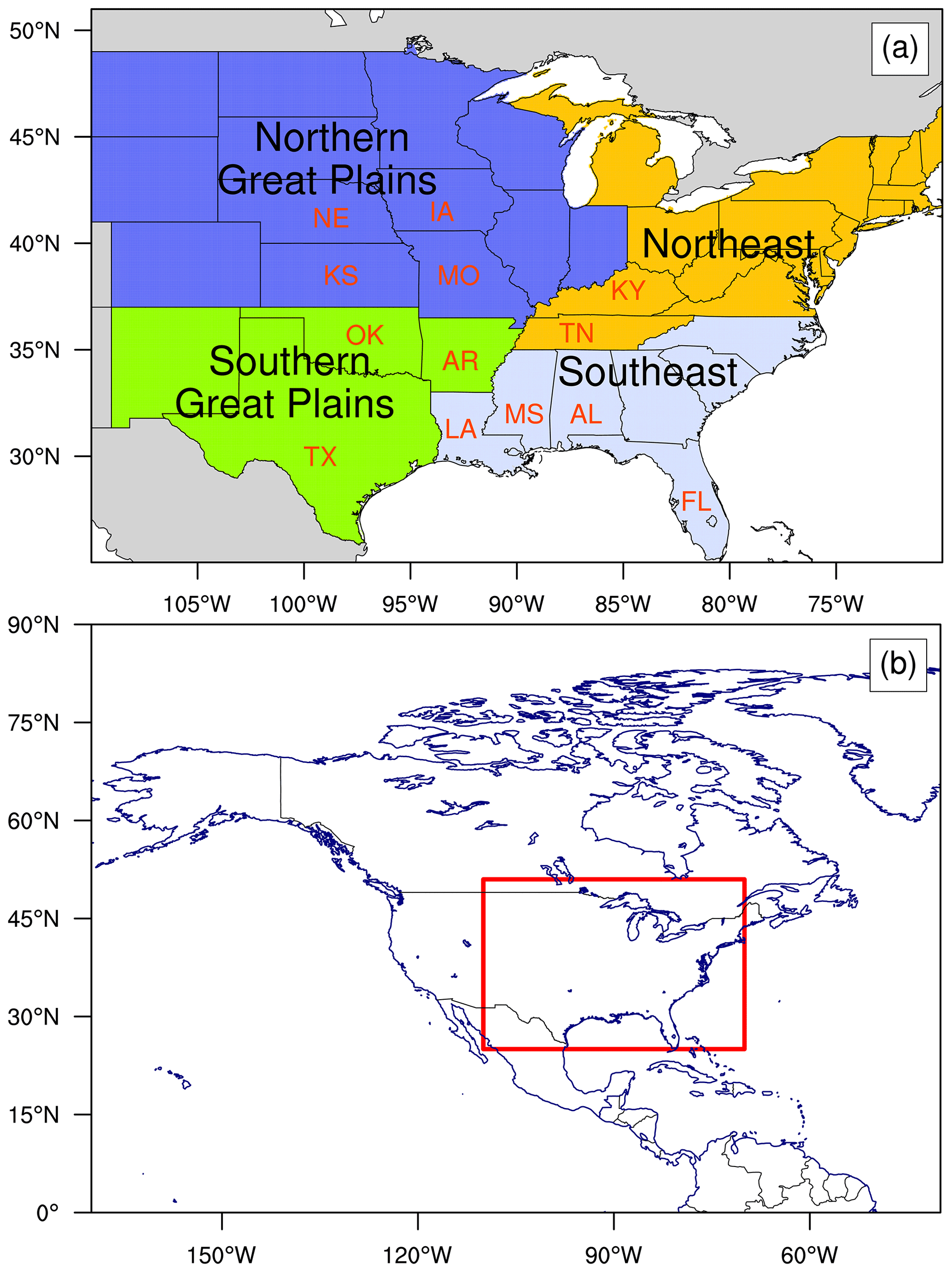
Figure 1(a) Data product domain and region definitions. Blue shading denotes the Northern Great Plains (NGP), green-yellow shading denotes the Southern Great Plains (SGP), light steel blue shading denotes the Southeast (SE), and orange shading denotes the Northeast (NE). The locations of some US states within each region are also labeled. TX is for Texas, OK for Oklahoma, KS for Kansas, NE for Nebraska, IA for Iowa, MO for Missouri, AR for Arkansas, LA for Louisiana, MS for Mississippi, AL for Alabama, TN for Tennessee, KY for Kentucky, and FL for Florida. (b) The location of the data product domain (red box) in North America.
2.2 Algorithm description
2.2.1 SL3D algorithm
The SL3D algorithm exploits GridRad ZH to classify each grid column with radar echoes into five categories: convective, precipitating stratiform, non-precipitating stratiform, anvil, and convective updraft (Starzec et al., 2017). SL3D identifies these five categories successively following the criteria listed in Table A2. We run the SL3D algorithm for 2004–2017 by using the re-gridded ERA5 melting level heights and GridRad ZH dataset described in Sect. 2.1. Figure 2e shows an example of the SL3D classification results based on GridRad ZH (Fig. 2d) at 2005-07-04T03:00:00Z. A sizable convective system with intense radar echoes and precipitation is observed in Kansas, and many isolated convection events are also observed in the Southeast. The SL3D classification results will be used in the following FLEXTRKR algorithm to identify convective core features (CCFs, continuous updraft or convective areas with precipitation > 0 mm h−1, which are used to indicate the existence of convective activity in the IDC definition; red regions in Fig. 3) and precipitation features (PFs, continuous updraft, convective, or precipitating stratiform areas with precipitation > 1 mm h−1; green areas in Fig. 3, which are used to denote the sizes of convective systems in the MCS and IDC definitions).
2.2.2 MCS and IDC identification and tracking
The FLEXTRKR algorithm was first developed and used by Feng et al. (2019) to track MCSs. In this study, we further update the algorithm so that it can identify and track MCS and IDC events simultaneously.
Figure 3 displays the schematic of FLEXTRKR (Feng et al., 2019). The first step is to identify cold cloud systems (CCSs; continuous areas with Tb<241 K) at each hour by applying a multiple Tb threshold “detect and spread” approach (Futyan and Del Genio, 2007). We search for cold cloud cores with Tb<225 K and spread the cold cloud cores to contiguous areas with Tb<241 K. Cloud systems that do not contain a cold cloud core but with Tb<241 K are also labeled as long as they can form continuous areas with at least 64 km2 (4 pixels). In addition, as described in Feng et al. (2019), CCSs that share the same coherent precipitation feature are combined as a single CCS. A coherent precipitation feature is defined as continuous areas with smoothed ZH at 2 km > 28 dBZ (if ZH is not available at 2 km, use ZH at 3 km instead if it is available) (Feng et al., 2019). We use a 5×5 pixel moving window to smooth ZH. Figure 2b shows an example of the CCSs identified in the first step based on Tb at 2005-07-04T03:00:00Z (4 July 2005, 3:00:00 UTC time). “Cloud 1” in Fig. 2b corresponds to a large area of low Tb in the central US (Fig. 2a).
In step 2, CCSs between two consecutive hours are linked if their spatial overlaps are > 50 %. “Linked” means the CCSs are considered to be from the same cloud systems. FLEXTRKR produces tracks by extending the link between two consecutive time steps to the entire tracking period, as shown in Fig. 3. Each track represents the life cycle of a cloud system. We calculate a series of CCS summary statistics associated with each track, such as CCS-based lifetime of the track (the duration of the track when CCSs are present), CCS area, CCS major axis length, CCS propagation speed, etc. In addition, SL3D classification (Fig. 2e) and Stage IV precipitation (Fig. 2c) within the tracked CCS are associated with the tracks and their merges and splits (described below). Then, we can obtain CCF and PF statistics of each track, such as convective and stratiform area, precipitation intensity and coverage, radar-derived echo-top heights, PF major axis length, CCF major axis length, intense convective cells (convective cells with column maximum reflectivity ≥ 45 dBZ and precipitation > 1 mm h−1; pink areas in Fig. 3, which are used to indicate intense convective activity in the following MCS definition), etc.
Merging and splitting refer to situations when two or more CCSs are linked to one CCS between consecutive hours (Figs. A1 and A2). A track associated with the largest CCS is defined as the main track (Fig. A3), and smaller tracks from merges or splits are regarded as parts of the main track when calculating PF and CCF statistics. In the algorithm, we require that a merge or split track associated with an MCS–IDC event must have a CCS-based lifetime of no more than 5 h. Otherwise, we treat it as an independent track.
The identification of MCS and IDC is based on the CCS, PF, and CCF statistics of the tracks. Following the definition of MCSs by Feng et al. (2019) (Fig. 4), we define a track as an MCS if it satisfies the following criteria: (1) there is at least one pixel of cold cloud core during the whole life cycle of the track, (2) CCS areas associated with the track surpass 60 000 km2 for more than 6 continuous hours, and (3) PF major axis length exceeding 100 km and intense convective cell areas of at least 16 km2 exist for more than 5 consecutive hours. Considering the lack of a strict and universal MCS definition (Geerts et al., 2017; Haberlie and Ashley, 2019; Pinto et al., 2015; Prein et al., 2017), we evaluate the impact of different MCS definition criteria on the data product in Sect. 4.4. For the non-MCS tracks, we further identify IDC with the following two criteria (Fig. 4): (1) a CCS with at least 64 km2 (4 pixels) is detected, and there is (2) at least 1 h during the life cycle of the track when PF and CCF are present (PF and CCF major axis lengths ≥ 4 km). In addition, for each IDC event, the CCS-based lifetime of associated merge and split tracks cannot surpass the lifetime of the IDC event. Here, the IDC criteria denote a low limit in convective signals that we can identify by using the FLEXTRKR algorithm and given source datasets. Potential uncertainties associated with the limit are discussed in Sect. 4.3.
Note that while we designate the term IDC to differentiate smaller convective storms from MCSs, there are sub-categories of deep convection within IDC. For example, multicellular convection systems that do not grow large enough or last long enough to meet our MCS definition are defined as IDC in our study, even though they are not necessarily “isolated.” Users of the data product can further separate sub-categories within IDC using the derived CCF statistics information to address specific science questions or research objectives.
Finally, the FLEXTRKR algorithm maps MCS–IDC track information back to the domain pixels. Figure 2f–i give an example of the pixel-level MCS–IDC information at 2005-07-04T03:00:00Z. Figure 2f displays the spatial coverages of MCS–IDC tracks at that time at pixel scale and the corresponding unique numbers of these tracks. From Fig. 2f, we know whether a pixel belongs to an MCS–IDC track and the number of the track if the pixel belongs to a track. We can further determine whether the track is an MCS or IDC event from Fig. 2g, which shows the types (MCS or IDC) of the tracks in Fig. 2f at pixel scale. Figure 2h and i are similar to Fig. 2f and g, respectively. The difference is that Fig. 2h and i only show pixels with precipitation > 1 mm h−1 in that hour. Together, the track-based CCS, PF, and CCF statistics of MCS and IDC events and the pixel-level dataset constitute the unified high-resolution MCS–IDC data product we develop in this study. Original Tb (Fig. 2a), Stage IV precipitation (Fig. 2c), GridRad ZH at 2 km (Fig. 2d), and GridRad-derived echo-top heights are also archived in the data product.
We run the FLEXTRKR algorithm separately for each year from 2004 to 2017. The starting time of each continuous tracking is 00:00 Z on 1 January, and the ending time is 23:00 Z on 31 December. Because winter has the fewest deep convection events, very few MCS–IDC events extend between two different years based on our investigation. Also, the lifetimes of MCS–IDC events are much shorter compared to our tracking period. Therefore, running FLEXTRKR separately for each year rather than continuously for the whole period has little impact on the MCS–IDC statistics.
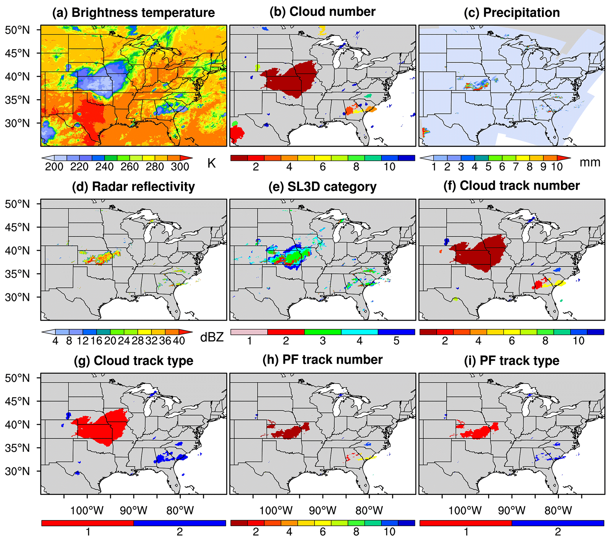
Figure 2FLEXTRKR pixel-level outputs at 03:00:00 Z on 4 July 2005. Panel (a) is satellite Tb. Panel (b) shows identified CCS labels. CCS labels are unique at each hour. Panel (c) is Stage IV hourly accumulated precipitation. Panel (d) is GridRad ZH at 2 km (if it is not available, ZH at 3 km is provided if it is available). Panel (e) is the SL3D classification results: (1) convective updraft, (2) convective, (3) precipitating stratiform, (4) non-precipitating stratiform, and (5) anvil. Panel (f) displays the track numbers to which pixels belong. Here, the track numbers are not the real values in the MCS–IDC data product. The track numbers should be unique throughout the whole running period. We adjust the track numbers here to make the figure clear. Similar to “PF track number.” Panel (g) gives information on whether the pixels belong to MCS (marked as 1) or IDC (marked as 2) tracks, which correspond to the tracks shown in (f). Panel (h) also displays the track numbers to which the pixels belong, but only for pixels with precipitation > 1 mm h−1. Panel (i) is like (g) but corresponds to (h). All these variables are stored in the FLEXTRKR hourly pixel-level output files.
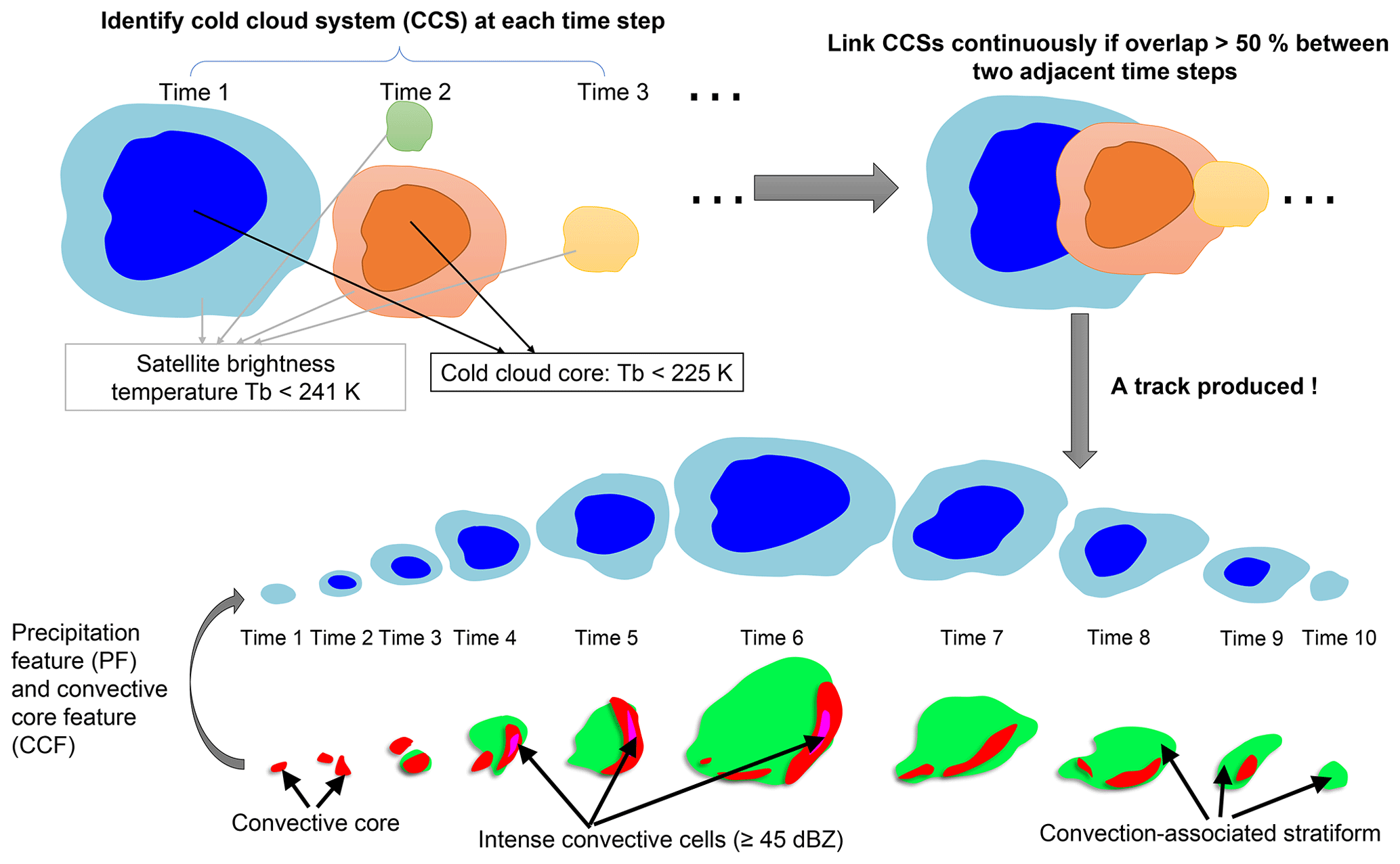
Figure 3Schematic of the FLEXTRKR algorithm highlighting three key steps in the algorithm: (1) the identification of CCS (upper left), (2) linking of overlapping CCSs (upper right), and (3) the tracking of both PF and CCF (bottom).
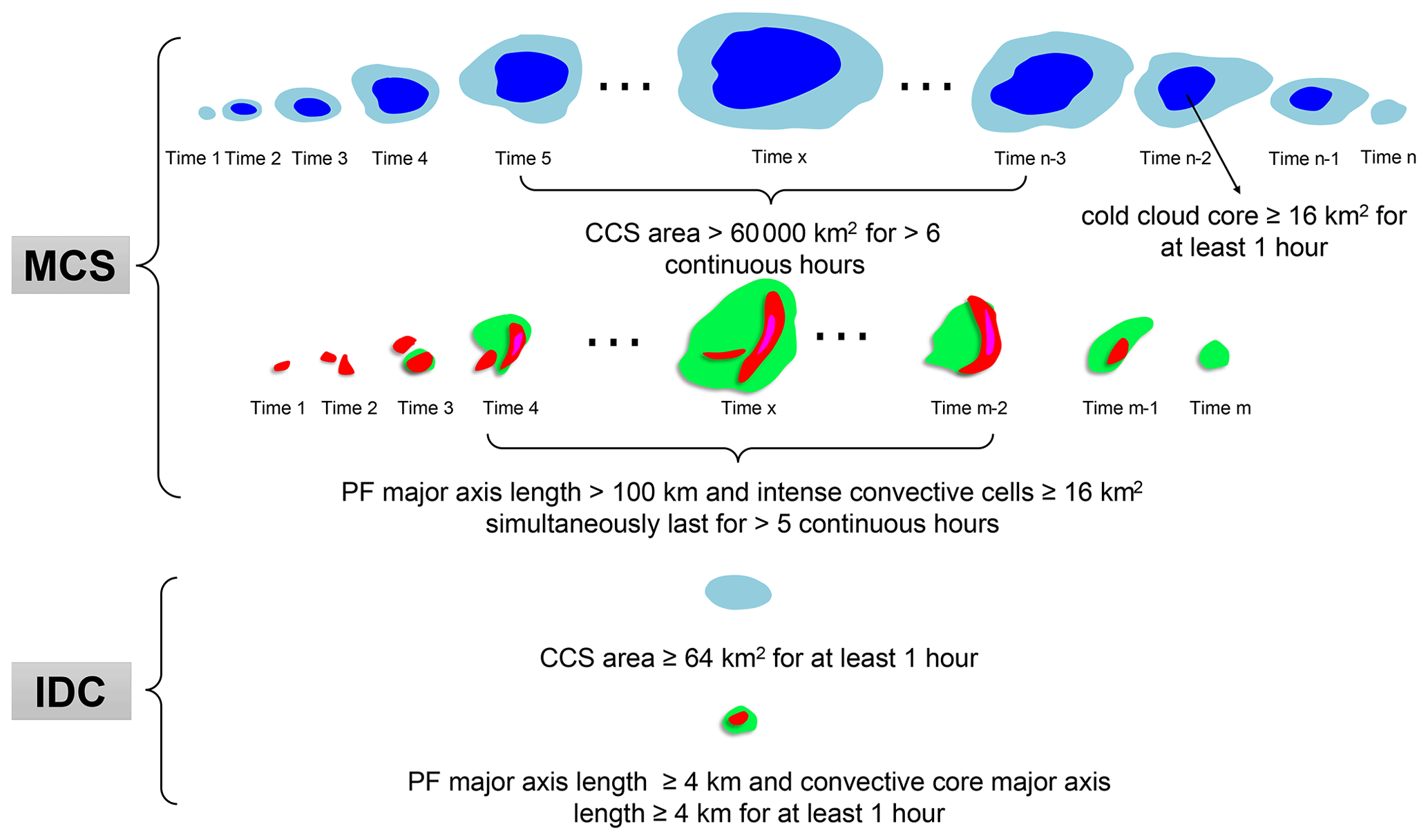
Figure 4Definition of MCS and IDC based on the FLEXTRKR algorithm shown in Fig. 3 and the specific threshold values used in the algorithm.
3.1 Climatological characteristics of MCS and IDC events
According to the MCS–IDC data product, we identify 45 346 IDC and 454 MCS events each year on average between 2004 and 2017 in our data product domain. Summer (June–August) has the most IDC and MCS events with average numbers of 25 073 and 212, while winter has the least with average quantities of 2545 and 37. During spring and autumn, there are 8543 and 9185 IDC events and 122 and 83 MCSs, respectively. The seasonal feature with the most occurrences of MCSs in winter and the least in summer is consistent with the results of Geerts (1998) in the Southeast US and Haberlie and Ashley (2019) over portions of the CONUS east of the Continental Divide (ECONUS).
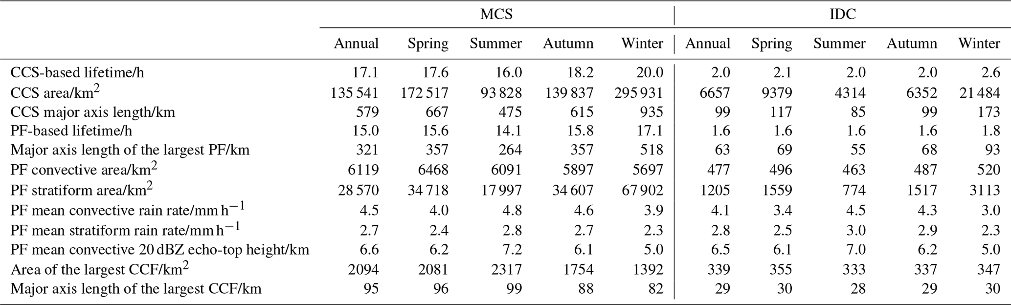
We compare the climatological characteristics of MCS and IDC events in Table 1. MCSs have much longer lifetimes than IDC, averaging 21.1 h (CCS-based) and 18.9 h (PF-based), compared to 2.1 h (CCS-based) and 1.7 h (PF-based) for IDC. Here, PF-based lifetime refers to the lifetime determined by the MCS–IDC PFs. Only those hours with a significant PF present (PF major axis length > 20 km for MCSs; ≥ 4 km for IDC) are counted during the life cycle of an MCS–IDC event, which represent the active convective period of a storm. We find that MCSs have the longest PF lifetime in winter (21.3 h) and the shortest in summer (17.9 h). In comparison, IDC has the longest PF lifetime in winter (1.9 h), but the summer lifetime (1.7 h) is comparable to spring and autumn. We examine the seasonal cumulative distribution functions (CDFs) of PF lifetimes for MCS and IDC events for 2004–2017 in Fig. A4. Results show winter has the largest fraction of MCS–IDC events with longer lifetimes compared to other seasons.
As expected, MCSs are much larger than IDC events in spatial coverage and precipitation area, as shown in Table 1 by the comparisons of CCS area, PF major axis length, PF convective or stratiform area, CCF area, and CCF major axis length. Generally, on average, winter MCS–IDC events are the largest in overall spatial coverage (both CCS and PF areas), while summer has the smallest. The larger and longer-lived MCSs in winter than in summer were also observed in the Southeast US in 1994–1995 by Geerts (1998). The remarkable seasonal difference in MCS–IDC overall spatial coverage is mainly due to stratiform areas. Convective areas are much smaller than stratiform areas. The PF stratiform area of MCSs in winter is 90 513 km2, 2.4 times larger than the area of 26 599 km2 in summer, but the PF convective area of MCSs in winter is 7293 km2, 14 % smaller than 8465 km2 in summer. Similarly, the IDC PF stratiform area in winter is 3182 km2, 2.8 times larger than 828 km2 in summer, while the IDC PF convective area in winter is 528 km2, slightly larger (9 %) than 483 km2 in summer. Unlike stratiform areas with the largest value in winter, convective activity is the most intense in summer as indicated by the PF mean convective 20 dBZ echo-top height in Table 1. The most intense convective activity reflects the strongest atmospheric thermal instability due to the strongest solar radiation in summer. We further confirm this point by investigating the MCS–IDC initiation time. As shown in Fig. A5, most MCS and IDC events initiate in the afternoon of summer when atmospheric instability is the strongest, consistent with Geerts (1998), who found warm-season MCSs generally initiated at 12:00–14:00 local time in the Southeast US.
Although MCSs are much larger than IDC events in spatial coverage, their mean convective 20 dBZ echo-top heights, which can be used to represent their mean convective intensities, are similar in Table 1. And their PF mean convective and stratiform rain rates are also comparable. PF mean convective and stratiform rain rates show significant seasonal variations for both MCS and IDC events. Summer MCS and IDC events have the largest rain rates, followed by autumn. Winter has the lowest rain rates compared to other seasons.
The high-resolution nature of the MCS–IDC data product enables a detailed examination of the 3-D evolutions of MCS–IDC events to investigate the relationships between atmospheric environments and MCS–IDC characteristics and to examine the impacts of MCSs and IDC on hydrology, atmospheric chemistry, and severe weather hazards. The data product can also be used to evaluate and improve the representation of MCS–IDC processes in weather and climate models. As an example of the application of the MCS–IDC data product, in Sect. 3.2, we investigate the contributions of MCS and IDC events to precipitation east of the Rocky Mountains for 2004–2017.
Table 1Annual and seasonal mean characteristics of MCS and IDC events in the data product domain for 2004–2017.
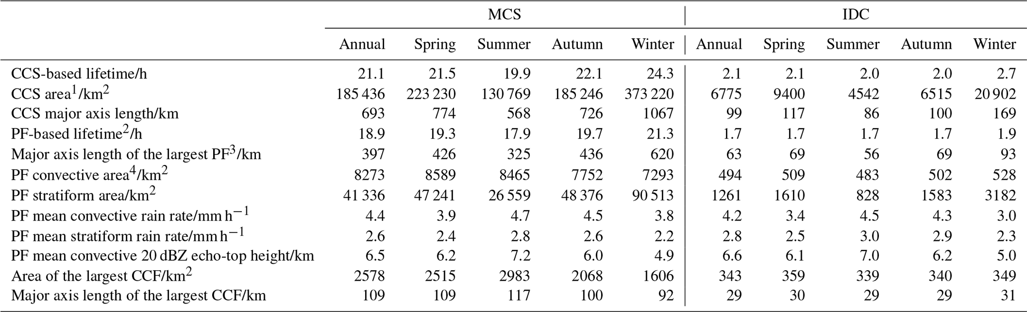
1 In this table, for hourly characteristics (all variables except for CCS-based lifetime and PF-based lifetime), we generally first calculate the average values of the characteristics during the duration of each MCS–IDC event except for the max dBZ echo-top heights, which are the maximum values of the attributes within the period. Then we calculate the mean values of the characteristics of all MCS–IDC events. For example, an MCS has a CCS-based lifetime of 10 h. During its duration, it has a CCS at each hour. We calculate the average CCS area during the 10 h, which is the average CCS area of the MCS. Then, we average all MCSs identified during a period to derive the values shown in this row. 2 Lifetimes of MCS–IDC events determined by PFs. Only count those hours of an MCS–IDC event with a significant PF present (PF major axis length > 20 km for MCSs; ≥ 4 km for IDC). 3 There can be multiple PFs and CCFs at a given time for an MCS–IDC event. “Largest” means only the largest PF or CCF is used in the calculation. 4 There can be multiple PFs and CCFs at a given time for an MCS–IDC event. If not specified, all PFs/CCFs are considered. For example, convective areas of all PFs at a given time are summed to represent the PF convective area of an MCS–IDC event at that time. Similarly, the convective rain rates of all PFs at the given time are averaged to represent the PF mean convective rain rate of the MCS–IDC at that time.
3.2 Precipitation characteristics from different sources
Here we only consider hourly data with precipitation > 1 mm h−1 (Feng et al., 2019). At 4 km resolution, precipitation less than 1 mm h−1 accounts for less than 19 % of the total precipitation, and the uncertainty of radar-derived precipitation at such low rainfall intensity is typically large. Including hourly data with precipitation ≤ 1 mm h−1 in the calculation will change the values shown in this study but will affect neither the comparison among MCS, IDC, and non-convective (NC) precipitation nor their spatial distribution patterns. Here, NC precipitation refers to precipitation not associated with any MCS or IDC events and is mainly from stratiform rain. Total precipitation is the sum of MCS, IDC, and NC precipitation. It is noteworthy that NC precipitation may contain some convection-associated rain due to the limitation of the source datasets and the algorithms used in this study. More relevant details are discussed in Sects. 3.2.3 and 4.
3.2.1 Annual spatial distributions of different types of precipitation
According to the MCS–IDC data product, the annual average total precipitation east of the Rocky Mountains in the US (US grid cells in Fig. 1) is 691 mm between 2004 and 2017 with a mean precipitation intensity of 3.6 mm h−1. MCSs contribute the most to the total precipitation with a fraction of 45 %, followed by NC (30 %) and IDC (25 %). And the mean precipitation intensities of MCSs (4.4 mm h−1) and IDC (3.8 mm h−1) are much larger than NC (2.7 mm h−1). Our MCS precipitation fraction (45 %) is higher than that (∼ 30 %) from Haberlie and Ashley (2019) over the ECONUS due to their different algorithms and stricter criteria to track and define MCSs.
Figure 5 displays the spatial distributions of annual mean precipitation amounts and intensities for different precipitation types for 2004–2017. We also calculate the distributions of the fractions of different types of precipitation in Fig. 6. MCS precipitation strongly affects the whole eastern US (105–70∘ W, MCS precipitation fractions: 46 % ± 12 %), especially in the south central US (MCS precipitation fractions: ∼ 60 %). The spatial distribution patterns of MCS annual precipitation amounts and fractions in Fig. 5 are similar to those from Haberlie and Ashley (2019), although their MCS precipitation fractions are generally lower than our results. IDC precipitation is concentrated in the SE and NE coastal areas, with peak values in Florida. NC precipitation is substantial in the eastern and southern regions with ample moisture supply and contributes over 35 % to the total precipitation across most of the NE region. The coastal area near Louisiana, which is significantly affected by all three types of precipitation, has the most total precipitation with annual amounts of over 1350 mm. The annual total precipitation amounts in most regions of SE also exceed 1050 mm due to MCS contributions. While the total precipitation amounts in most regions of Florida are also over 1050 mm, they are mainly attributed to IDC.
The spatial patterns of precipitation intensities are somewhat different from those of precipitation amounts (Fig. 5). Generally, the southern regions, especially in the coastal areas, have larger precipitation intensities than the northern areas. The MCS precipitation intensities are the largest in Texas, Louisiana, Oklahoma, and Kansas, significantly shifting west compared to MCS precipitation amounts. Unlike IDC precipitation amounts concentrating in the SE and NE coastal areas, IDC precipitation intensities are the largest over the SGP and SE. IDC precipitation intensities over the NE are much smaller compared to the SGP and SE, similar to NC precipitation intensities. We summarize the annual mean precipitation amounts and intensities of different types of precipitation in the NGP, SGP, SE, and NE in Table A3.
The distributions of MCS–IDC precipitation amounts are mainly determined by the distributions of MCS–IDC hours (Figs. 5 and 7). Here, the MCS–IDC hour of a grid cell during a period is the number of hours when any MCS–IDC events produce > 1 mm hourly accumulated rainfall in the grid cell. The distributions of MCS–IDC precipitation intensities, although not the main factor, can also affect the distributions of MCS–IDC precipitation amounts. For example, the maximum MCS hours are located around Missouri (Fig. 7a), but the maximum MCS precipitation amount is in the coastal area of Louisiana (Fig. 5c). The larger MCS precipitation intensities in the southern regions contribute more to the MCS precipitation amount in the southern US. In addition, a large number of IDC events (IDC hours > 60 h yr−1) occur in the NE region along the Appalachian Mountains (Fig. 7b), but IDC in that region only contributes to 20 %–30 % of the total precipitation amount (Fig. 6b) due to the low precipitation intensities (Fig. 5f).
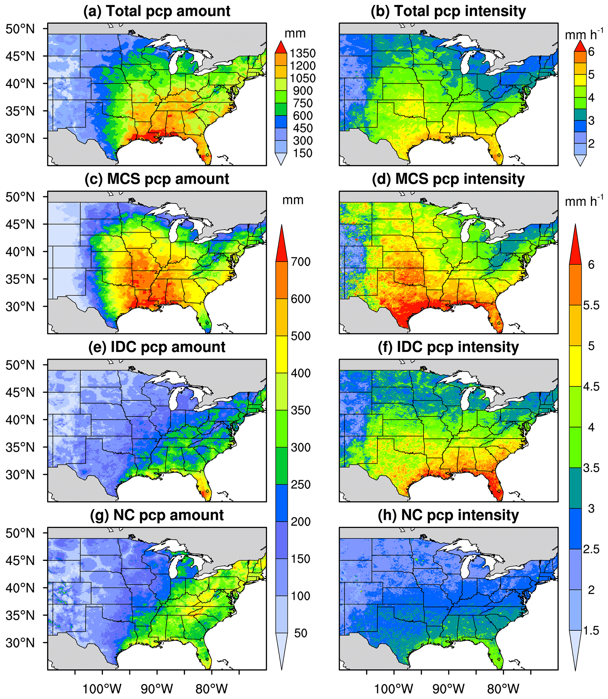
Figure 5Distributions of annual mean precipitation amounts (a, c, e, g) and intensities (b, d, f, h) for different types of precipitation for 2004–2017. Panels (a) and (b) are for total precipitation, (c) and (d) are for MCS precipitation, (e) and (f) are for IDC precipitation, and (g) and (h) are for NC precipitation. We only include hourly data with precipitation > 1 mm h−1 in the calculation.
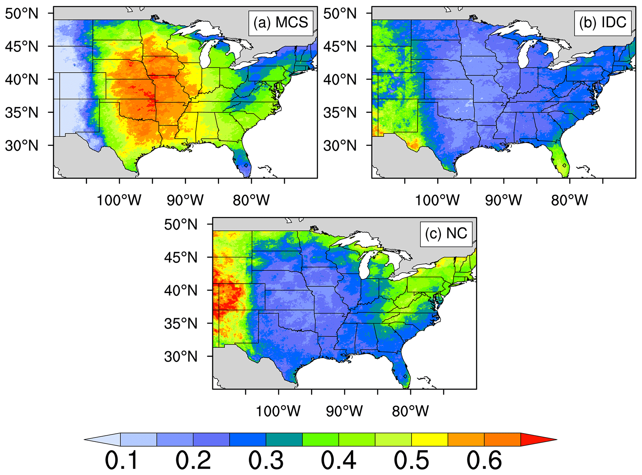
Figure 6Distributions of the fractions of different types of precipitation (MCS, IDC, NC). Here, precipitation refers to annual mean values for 2004–2017. We exclude hourly data with precipitation ≤ 1 mm h−1 in the calculation.
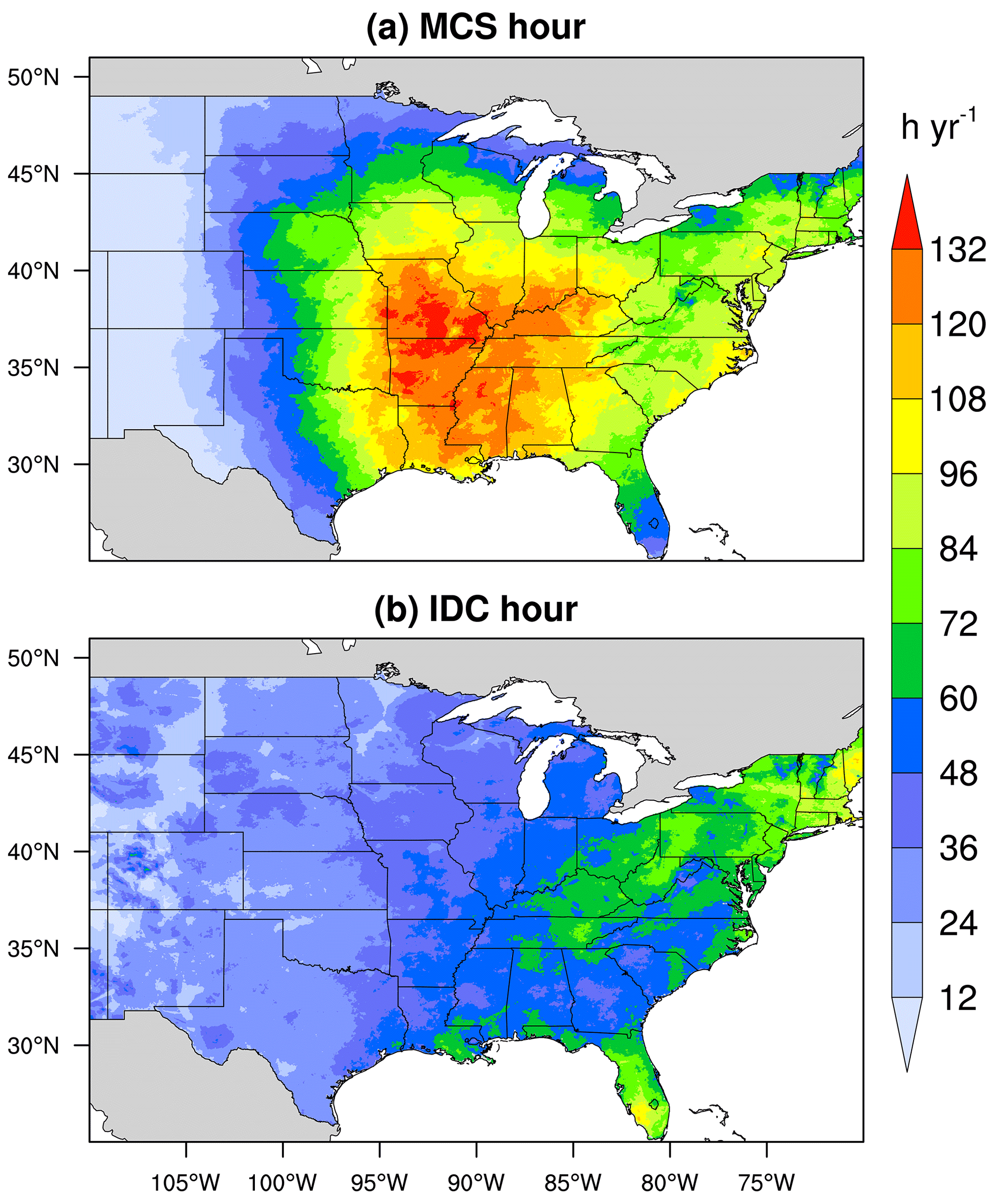
Figure 7Spatial distributions of annual mean MCS–IDC hours for 2004–2017. Panel (a) is for MCS, and (b) is for IDC. The annual mean MCS–IDC hour of a grid cell is the number of hours per year when any MCS–IDC events produce > 1 mm hourly accumulated rainfall in the grid cell.
3.2.2 Seasonal spatial distributions of different types of precipitation
Figures 8, A6, and A7 display the mean seasonal distributions of precipitation amounts, precipitation fractions, and precipitation intensities for different types of precipitation in 2004–2017. The MCS precipitation center migrates northwards from Arkansas in spring to northern Missouri and Iowa in summer, followed by a southward migration to Louisiana in autumn, and finally to Mississippi and Alabama in the Southeast (Fig. 8e–h) in winter. The seasonal shift of the MCS precipitation center agrees with the study of Haberlie and Ashley (2019), showing different MCS precipitation distributions between warm and cold seasons over the ECONUS. Spring and summer have much larger MCS precipitation amounts (∼ 100 mm) than autumn (∼ 62 mm) and winter (∼ 50 mm). The mean MCS precipitation amount in spring is close to that in summer. However, the total number of identified MCSs in summer (212) is much higher than that in spring (122), as discussed in Sect. 3.1; the mean MCS precipitation intensity in summer (5.2 mm h−1) is also larger than that in spring (4.1 mm h−1) (Fig. A7). The inconsistency is because MCSs in spring occur in more favorable large-scale environments with strong baroclinic forcing and low-level moisture convergence (Feng et al., 2019; Song et al., 2019). As a result, spring MCSs are larger and longer-lasting, and they produce more rainfall per MCS event compared to those in summer (Table 1), compensating for the fewer number of MCS events and lower precipitation intensities in spring. The fractions of MCS precipitation amounts are generally > 35 % over the Northern and Southern Great Plains in spring and summer and can reach up to over 70 % within the MCS precipitation center (Fig. A6a–b). The results are roughly consistent with Fritsch et al. (1986), which showed that MCSs accounted for about 30 %–70 % of the warm-season (April–September) precipitation over much of the region between the Rocky Mountains and the Mississippi River. The results are also consistent with Haberlie and Ashley (2019), showing MCS precipitation fractions generally > 30 % with a peak > 60 % over the Great Plains between May and August. Due to the low precipitation amounts of IDC and NC, the fractions of MCS precipitation amounts in autumn and winter are also large, showing over 50 % within the MCS precipitation center (Fig. A6c–d).
The IDC precipitation amounts reach a maximum in summer, centered in the coastal areas of the SE, where IDC precipitation contributes to more than 40 % of the total precipitation amounts (Figs. 8i–l and A6e–h). Winter has the least IDC precipitation. Areas of high IDC precipitation do not show much seasonal variability, suggesting that IDC is constrained by local conditions such as moisture availability, local solar radiation, and land–atmosphere interactions. The NC precipitation amount also peaks in summer, followed by autumn, particularly in the NE (Fig. 8m–p). However, because both MCS and IDC precipitation amounts are very high in summer, the fraction of the NC precipitation amount in summer (28 %) is smaller than that of winter (32 %) (Fig. A6i–l). Winter NC precipitation center occurs in the SE coastal areas (Fig. 8p).
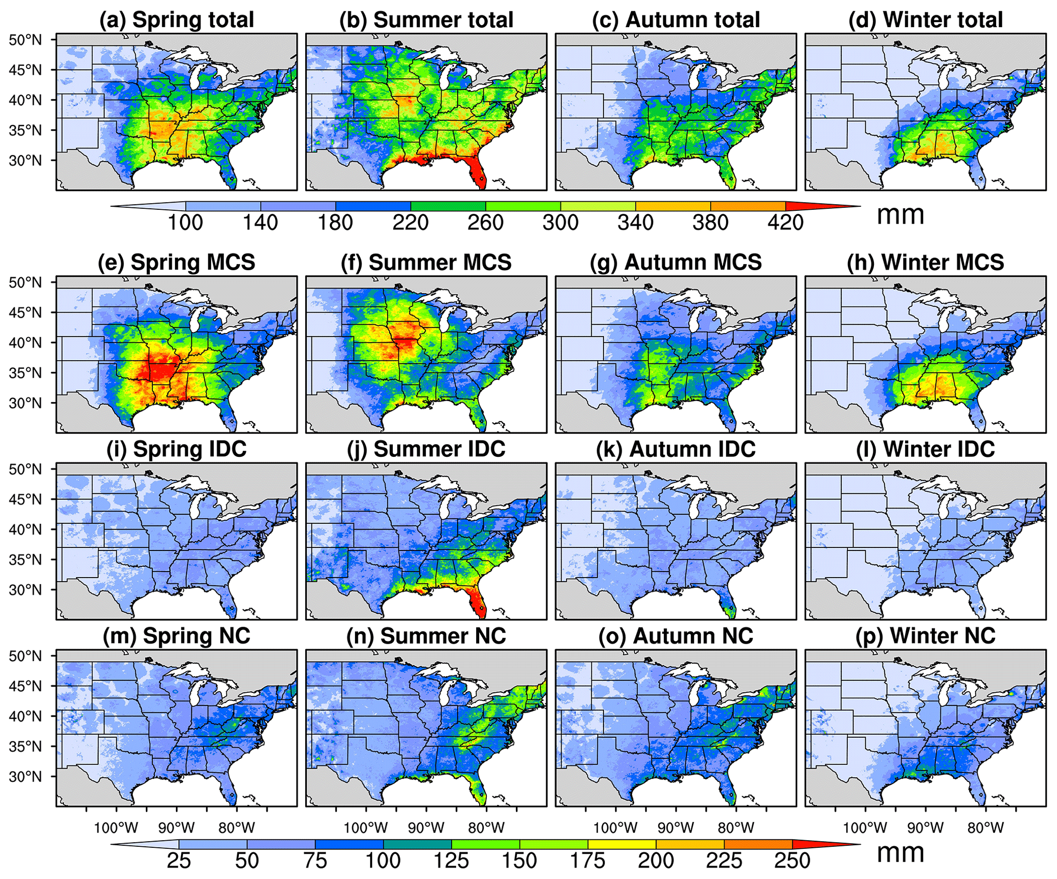
Figure 8Distributions of annual mean seasonal precipitation amounts for different types of precipitation for 2004–2017. The first row is for total precipitation, the second for MCS precipitation, the third row for IDC precipitation, and the fourth row for NC precipitation. The first column shows spring precipitation, the second column summer, the third column autumn, and the fourth column winter. MCS, IDC, and NC precipitation values share the same label bar. We exclude hourly data with precipitation ≤ 1 mm h−1 in the calculation.
The precipitation intensities of all three types peak in summer and reach minimums in winter (Fig. A7). In each season, precipitation intensities in the south are larger than those in the north except for MCS precipitation intensities in summer, which maximize in Oklahoma. We summarize the mean seasonal precipitation amounts and intensities of different types of precipitation over the four climate regions of Fig. 1 in Table A4.
3.2.3 Diurnal cycles of different types of precipitation
Figure 9 shows the monthly mean diurnal cycles of precipitation amounts from MCSs, IDC, and NC in the NGP, SGP, SE, and NE, respectively. Generally, MCS precipitation peaks during nighttime in the NGP, SGP, and NE. The seasonal shift of the peaks from spring in the SGP to summer in the NGP reflects the northward migration of the MCS precipitation center in the Great Plains (Fig. 8e and f).
The SE has significantly different diurnal cycles of MCS precipitation from other regions. In spring, SE MCS precipitation is mainly located in the western areas (Fig. 8e), showing similar diurnal characteristics as the SGP MCS precipitation but with peaks in the early morning and late afternoon (Fig. 9d and g). Besides, the SGP MCS precipitation peaks in May (Fig. 9d), while SE peaks in April (Fig. 9g), suggesting that the MCS precipitation center first appears in the western SE regions (Alabama, Mississippi, and Louisiana) in April and then moves northwards to Arkansas in May. In summer, the SE MCS precipitation diurnal cycles are more like those of IDC (Fig. 9g and h), peaking in the late afternoon and much different from those in the Great Plains. The significantly different precipitation diurnal variations between the Great Plains and SE were also identified by Haberlie and Ashley (2019). We find that most summer MCS precipitation over the SE occurs near the coastal areas (Fig. 8f), far from the MCS precipitation center in northern Missouri and Iowa, suggesting either a different MCS genesis mechanism in the SE from those in the SGP and NGP (Feng et al., 2019) or long-duration deep convective systems showing MCS characteristics (Geerts, 1998). In autumn, the SE MCS precipitation peaks in the morning (Fig. 9g). The diurnal cycle of MCS precipitation in September shows mixed features of summer and autumn with peaks in both the morning and the afternoon. In winter months, the diurnal cycle of the SE MCS precipitation shifts from the autumn feature to the spring feature, with peaks shifting from the morning to the afternoon. The distinct diurnal cycles of SE MCS precipitation in different seasons in Fig. 9g are roughly consistent with the corresponding seasonal diurnal variations in MCS occurrence frequencies from Geerts (1998), where the occurrence time of an MCS was defined as the central time between the initiation and decay of the MCS.
The diurnal cycles of IDC precipitation are consistent in all regions (Fig. 9b, e, h, and k), peaking in the late afternoon in summer (Tian et al., 2005), again reflecting the impact of local instability driven by the solar forcing on IDC development. NC precipitation (Fig. 9c, f, i, and l) shows some diurnal cycle characteristics similar to IDC precipitation. It may be caused by the limitation of the temporal resolution of the datasets used in the FLEXTRKR algorithm. Weak IDC events that are shorter than 1 h could be missed by GridRad in identifying CCFs, as GridRad ZH only considers reflectivities within ±3.8 min of the analysis time. These weak IDC could be aliased to NC precipitation, therefore showing some similar diurnal cycles as IDC. Another possible reason is that the FLEXTRKR algorithm may miss some parts of IDC clouds with Tb≥241 K, which are then classified as NC, so the NC precipitation exhibits some IDC characteristics.
The monthly diurnal cycles of precipitation intensities for MCSs, IDC, and NC are generally similar among all regions, peaking in the late afternoon and early morning in the warm season (Fig. A8).
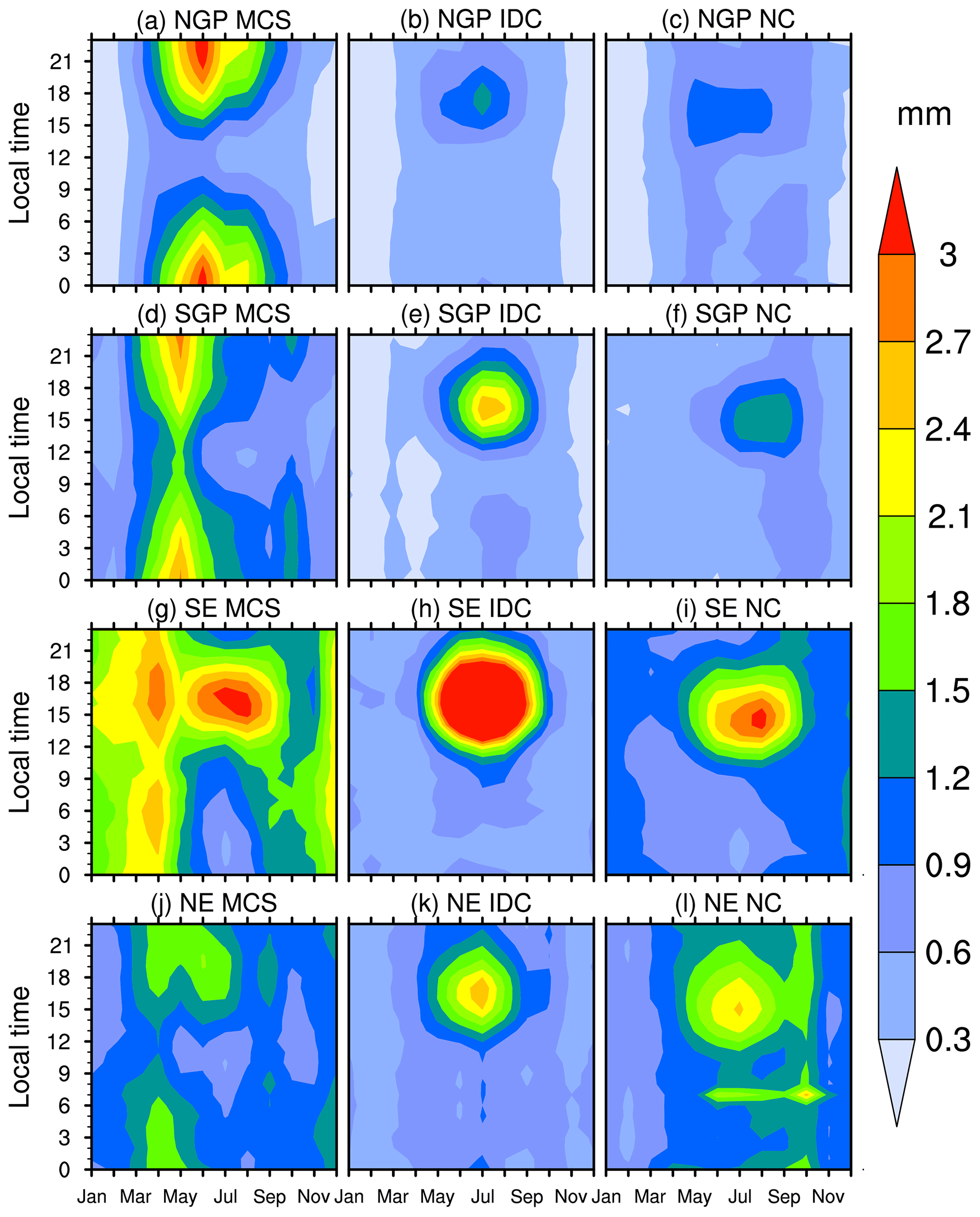
Figure 9Monthly mean diurnal cycles of precipitation amounts from MCSs (a, d, g, j), IDC (b, e, h, k), and NC (c, f, i, l) in the NGP (a, b, c), SGP (d, e, f), SE (g, h, i), and NE (j, k, l) during 2004–2017.
4.1 Uncertainties from source datasets
The NCEP/CPP L3 4 km Global Merged IR V1 Tb dataset has been view-angle-corrected and re-navigated for parallax (Janowiak et al., 2001) to reduce errors. However, the US continent is covered by two series of geostationary IR satellites (GOES-W and GEOS-E). During the production of the Tb dataset, the value with the smaller zenith angle is adopted when duplicate data are available in a grid pixel. Measurements from different satellites may be inconsistent. Janowiak et al. (2001) suggest this type of inconsistency to be considered minor.
For the GridRad radar dataset, some bad volumes have been removed during the production of GridRad ZH. We further filter out potential low-quality observations, scanning artifacts, and non-meteorological echoes from biological scatters and artifacts following the approaches of Homeyer and Bowman (2017). However, there is another source of error from anomalous propagation caused by non-standard refractions of radar signals in the lower atmosphere, which cannot be mitigated during the filtering procedure. Non-standard refractions can result in underestimation or overestimation of the true radar beam altitude, thus affecting the location of radar reflectivity for binning. Estimating the corresponding uncertainties is out of the scope of this study. However, anomalous propagation is typically limited to radar beams traveling long distances in the boundary layer (Homeyer and Bowman, 2017).
Stage IV precipitation is a mosaic of precipitation estimates based on a combination of NEXRAD and gauge data from 12 RFCs. Therefore, the errors of Stage IV are from several sources, such as inherent NEXRAD biases, radar quantitative precipitation estimate (QPE) algorithm biases, bad gauge data removal inconsistency among different RFCs, multisensory processing algorithm inconsistency among different RFCs, and mosaicking border discontinuities (Nelson et al., 2016). The most severe errors occur in the western US, where NEXRAD data are limited, and a gauge-only rainfall estimation algorithm is used (Nelson et al., 2016; Smalley et al., 2014). Hence our data product has a geographical focus east of the Rocky Mountains, with the best NEXRAD coverage in the US. After regridding the Stage IV precipitation into our 4 km domain, we further manually filter out certain “erroneous precipitation” hours and set all precipitation in those hours to missing values. Erroneous precipitation is defined as sudden appearance and disappearance of a large contiguous area (> 4800 km2) with intense precipitation (> 40 mm h−1) (Fig. A9), which is physically not possible. There are 40 h in total in the period 2004–2017 containing such erroneous precipitation.
As the FLEXTRKR algorithm is applied to a combination of three independent types of remote sensing datasets, we identify the most robust MCS–IDC events satisfying all the criteria based on the three datasets. It reduces the potential false classification of tracks as MCSs or IDC based on any single dataset. And to consider the potential error of ERA5 melting level heights, we require ZH≥45 dBZ above (Zmelt+1) km for convective classification in the SL3D algorithm (Table A2).
4.2 The impact of missing data
In the CCS identification step of the FLEXTRKR algorithm, we require the fraction of missing satellite Tb in the domain at each hour to be less than 20 %. Otherwise, the hour is excluded from our data product. During 2004–2017, we excluded 716 h with missing satellite Tb data, accounting for less than 0.6 % of the total period. The year with the most missing satellite data is 2008, with 206 missing hours (2.3 %), followed by 2004 with 154 h (1.8 %). All other years have no more than 57 missing hours. During the link procedure of the FLEXTRKR algorithm, we search the next hour if a missing hour is encountered, as long as the time gap between the two “linked” hours is less than 4 h. Otherwise, we start new tracks from the next available hour. This method aims to reduce the impact of the missing hours. Considering the high completeness of the satellite Tb data in 2004–2017, we conclude that the missing satellite data have little effect on the data product.
We show the distribution of the fractions of valid Stage IV precipitation data in 2004–2017 in Fig. A10. The fractions are over 97 % for all grid cells of the US in the domain. Most grid cells in the US have less than 2 % missing hours, which should have a negligible impact on the data product.
Figure A11 shows the fractions of available GridRad reflectivity data from 2004 to 2017 between 1 and 12 km a.s.l. The fractions are relatively high over the majority of the troposphere except for 1 km a.s.l. Based on the criteria of the SL3D algorithm, ZH at 1 km is rarely used and can be easily substituted by ZH at 2 km. Generally, GridRad has good spatial coverage during the period, with most grid cells east of the Rocky Mountains having fractions > 90 % between 2 and 9 km and 80 % between 10 and 12 km. The completeness of the GridRad dataset is relatively lower compared to the satellite Tb and Stage IV precipitation datasets, and GridRad ZH is a crucial variable in the SL3D classification and MCS–IDC identification. Therefore, the missing data of GridRad ZH should have some impacts on our data product. However, as an advanced long-term high-resolution 3-D radar reflectivity dataset, GridRad is valuable for constructing a climatological MCS–IDC data product.
4.3 Temporal resolution limitation of the source datasets
As we discussed in Sect. 3.2.3, the diurnal cycles of NC precipitation show some possible aliasing from IDC precipitation. Some weak IDC events are so short that the hourly data cannot properly capture their occurrence, especially for GridRad ZH, which only includes reflectivities within ±3.8 min of each hour. We calculate the cumulative distribution functions of PF-based lifetimes for MCS and IDC events and their associated precipitation in the data product for 2004–2017, as shown in Fig. 10. About 75 % of IDC events have a PF-based lifetime of 1 h. Therefore, it is almost certain that we miss some IDC events shorter than 1 h in the data product. Here we give an estimate of the probability p that a given IDC event with a convective signal duration of x minutes is detected by radar, as expressed below:
where the numerator is the time window of GridRad observation in each hour, and x is the duration of the IDC event. The detection probability is only about 25 % when x=30 min. To obtain a detection probability of 50 %, we require x≥45 min. Hence, we cannot assess the distribution of IDC convective signals with durations less than 1 h using the currently available datasets. Higher-resolution datasets, such as individual NEXRAD radar data, which typically have an update cycle of 4–5 min, are necessary to derive the information. However, as shown in Fig. 10, we find that precipitation from IDC events with a 1 h PF lifetime only accounts for about 10 % of the total IDC precipitation. Therefore, IDC events with PF lifetimes less than 1 h should have a relatively small impact on precipitation.

Figure 10Cumulative distribution functions of PF-based lifetimes for MCS and IDC events and their associated precipitation in the data product domain for 2004–2017. The red solid line is for the number of MCSs, the red dashed line for MCS-associated precipitation, the blue solid line for the number of IDC events, and the blue dashed line for IDC-associated precipitation.
4.4 The impact of MCS and IDC definition criteria
The separation between MCSs and long-lasting IDC events is somewhat fuzzy (Feng et al., 2019; Geerts et al., 2017; Haberlie and Ashley, 2019; Pinto et al., 2015; Prein et al., 2017). Here, we briefly examine the impact of different MCS–IDC definition criteria on the data product. We change the definition of MCSs to relax the CCS and PF size and duration thresholds. Specifically, the second and third criteria listed in Sect. 2.2.2 are modified as follows: (2) CCS areas associated with the track surpass 40 000 km2 for more than 4 continuous hours and (3) PF major axis length exceeding 80 km and intense convective cell areas ≥ 16 km2 exist for more than 3 consecutive hours. And we also require that each merge or split track associated with MCS–IDC events has a CCS-based lifetime of no more than 3 h. We keep the definition of IDC the same as described in Sect. 2.2.2, which is a limit for IDC that we can identify based on the source datasets.
By using the new definition, as expected, the lifetimes and spatial coverages of MCSs are reduced, and those of IDC change little because most IDC events cannot satisfy the new MCS criteria (Tables 1 and A5). The annual number of MCSs identified in 2004–2017 increases from 454 to 857. The number increases from 122 to 207 in spring, 212 to 434 in summer, 83 to 151 in autumn, and 37 to 62 in winter. As PF-based lifetimes of MCS–IDC events in summer are the shortest (Table 1), the new definition has the most significant impact in summer. The annual number of IDC decreases from 45 346 to 45 225. Reducing the merge or split lifetime limit retains more independent IDC events, which is the reason why the decrease in the number of IDC events is smaller than the increase in the number of MCSs. Annual mean MCS precipitation east of the Rocky Mountains increases from 313 to 353 mm, while IDC precipitation decreases from 170 to 130 mm. The fraction of MCS precipitation only increases by 6 % (from 45 % to 51 %), compared to the almost doubling of MCS number (from 454 to 857), suggesting the MCS definition in the original data product is capable of capturing most of the important MCSs with heavy precipitation. Similar to MCS numbers, summer has the most increase in MCS precipitation amount, from 100 to 119 mm. And annual mean MCS and IDC precipitation intensities decrease slightly as MCS precipitation intensities are somewhat larger than IDC in most regions (Tables A3, A4, A6, and A7). We summarize the regional precipitation statistics of the NGP, SGP, SE, and NE based on the new definition in Tables A6 and A7.
Although the new definition changes the absolute values of MCS–IDC characteristics, the contrast between MCS and IDC events is still present. The new definition has small impacts on the spatial distribution patterns of MCS–IDC precipitation. And NC precipitation characteristics are almost the same as before. Therefore, our original definition captures the essential characteristics of MCS and IDC events. In addition, the original data product is complete and flexible. We store all criteria variables of MCS–IDC events in the data product. Users can easily change the definition of MCSs and switch between tracks that are attributed to MCS and IDC without re-running the FLEXTRKR algorithm. There is no need to change the “track” and “merge” lifetime criteria as we do above because they have little impact on the climatological characteristics of MCS and IDC events.
4.5 Recommendations for the usage of the MCS–IDC data product
Considering the limitations and uncertainties mentioned above, we generally recommend using the data product for observational analyses and model evaluations of convection statistics and characteristics over relatively long periods such as a month, a season, or longer to fully take advantage of the long-term dataset, although analysis of individual weather events is also possible as supported by the hourly temporal resolution of the data product. In addition, since the completeness and quality of the source radar dataset degrade dramatically beyond the US border and over the Rocky Mountains (Fig. A11), we recommend the usage of the data product within the CONUS east of the Rocky Mountains to alleviate the impact of the termination of MCS–IDC tracks due to poor radar coverage and missing radar data beyond their maximum scan range.
Detailed investigation of a short period or a specific MCS–IDC event is acceptable, but caution should be taken when encountering missing data around the track during the period. Due to the complexity of the algorithms used to develop the data product, it is difficult to quantify the impact of missing data on the MCS–IDC track. Therefore, we do not recommend examining a specific MCS–IDC track if there are too many missing data (precipitation, Tb, or ZH) along the track. Users planning to apply the data product for a specific case study should examine the availability of the source data first, which are also stored in the data product except for 3-D ZH due to the large data volume. Users can access the original 3-D ZH at https://rda.ucar.edu/datasets/ds841.0/ (last access: 2 January 2020) (Table A1).
Lastly, although our sensitivity test in Sect. 4.4 shows that precipitation characteristics are similar between two different sets of MCS–IDC definition criteria, we still recommend users conduct further sensitivity tests and examine the impact of different definition criteria on the results if the data product is applied to other studies, such as the effects of MCS and IDC events on atmospheric circulation, environmental conditions associated with the initiation and evolution of MCS and IDC events, and MCS–IDC-associated weather hazards.
The high-resolution (4 km hourly) MCS–IDC data product and the corresponding user guide document are available at https://doi.org/10.25584/1632005 (Li et al., 2020). The original format of the data files is NetCDF-4, and we archive them as compressed files for each year so that the data product is easily accessible. The user guide contains a brief explanation about the approach to develop the data product and a detailed description of the data file content to help users understand the data product.
Here we present a unified high-resolution (4 km, hourly) data product that describes the spatiotemporal characteristics of MCS and IDC events from 2004 to 2017 east of the Rocky Mountains over the CONUS. We produce the data product by applying an updated FLEXTRKR algorithm to the NCEP/CPP L3 4 km Global Merged IR V1 Tb dataset, ERA5 melting level heights, 3-D GridRad radar reflectivity dataset, and Stage IV precipitation dataset. Climatological features of the MCS and IDC events from the data product are compared, with a focus on their precipitation characteristics. Consistent with our definitions of MCSs and IDC in the FLEXTRKR algorithm, we find that MCSs have much broader spatial coverage and longer duration than IDC events. While there are many more frequent IDC occurrences than MCSs, the mean convective intensities of IDC events are comparable to those of MCSs. MCS and IDC events both contribute significantly to precipitation east of the Rocky Mountains but with distinct spatiotemporal variabilities. MCS precipitation affects most regions of the eastern US in all seasons, especially in spring and summer. The MCS precipitation center migrates northwards from Arkansas in spring to northern Missouri and Iowa in summer, followed by a southward migration to Louisiana in autumn, and finally to Mississippi and Alabama in the Southeast in winter. IDC precipitation mostly concentrates in the Southeast in summer. IDC precipitation shows a significant diurnal cycle in summer months with a peak around 16:00–17:00 local time over all regions east of the Rocky Mountains. In contrast, MCS precipitation peaks during nighttime in spring and summer for most regions except for the Southeast, where MCS precipitation peaks in the late afternoon in summer, similar to IDC precipitation. Lastly, we analyze the potential uncertainties of the data product and the sensitivity of the dataset to MCS definitions and give our recommendations for the usage of the data product. The data product will be useful for investigating the atmospheric environments and physical processes associated with convective systems; quantifying the impacts of convection on hydrology, atmospheric chemistry, severe weather hazards, and other aspects of the energy, water, and biogeochemical cycles; and improving the representation of convective processes in weather and climate models.
Table A1Summary of source datasets used to develop the MCS–IDC data product.
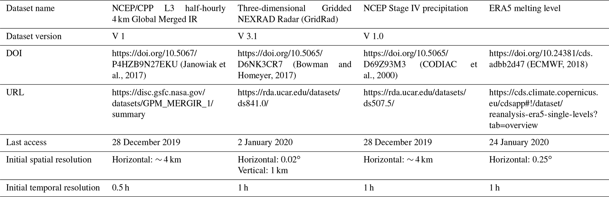
Table A2The classification criteria of the Storm Labeling in Three Dimensions (SL3D) algorithm in this study.
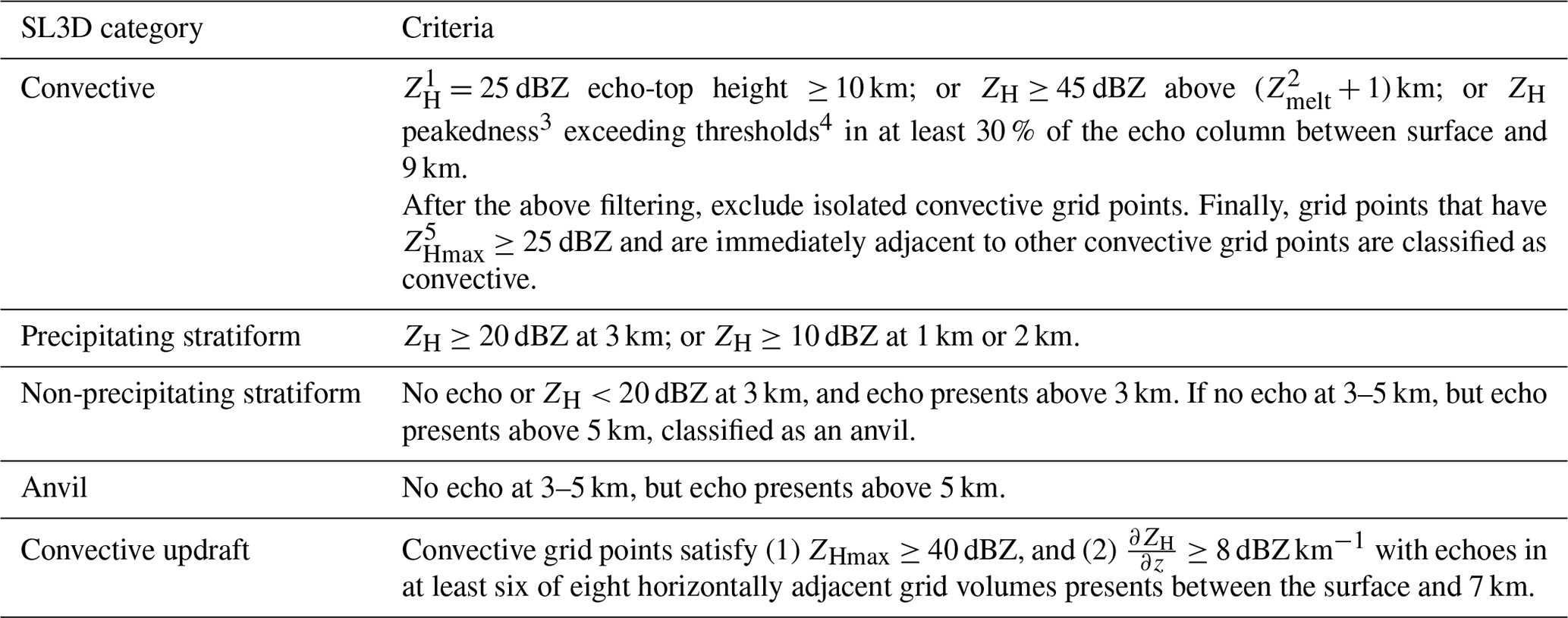
1 ZH: logarithmic radar reflectivity. 2 Zmelt: melting level height. If temperatures at different vertical levels within a grid column are all below zero, there is no melting level. In this situation, we set . 3 Peakedness is the difference between the ZH of the grid point being evaluated and the median ZH of a horizontal 12 km radius around the point. 4 Threshold . 5 ZHmax denotes column max reflectivity.
Table A3Annual mean precipitation amounts and intensities for different types of precipitation in different regions of the US for 2004–2017.
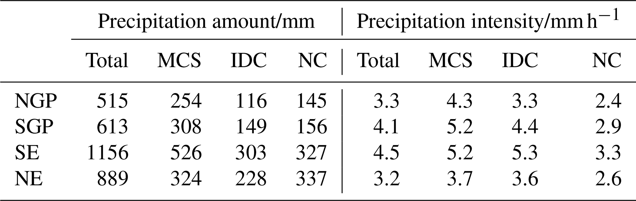
Table A4Annual mean seasonal precipitation amounts and intensities for different types of precipitation in different regions of the US for 2004–2017.
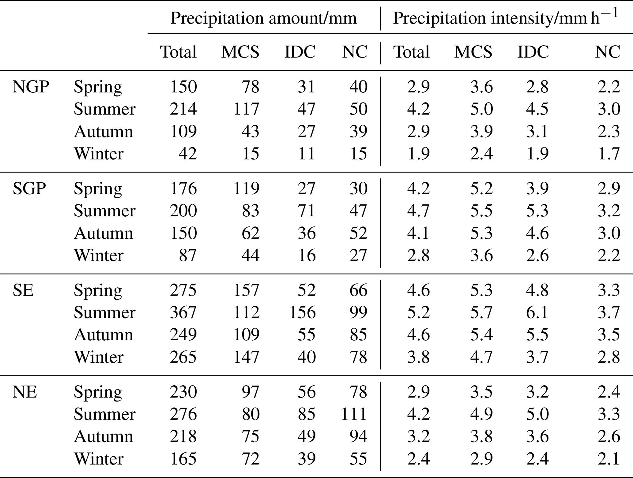
Table A5Annual and seasonal mean characteristics of MCS and IDC events in the data product domain for 2004–2017 by using the new MCS definition*.
* Refer to Sect. 4.4 for the new MCS definition.
Table A6Annual mean precipitation amounts and intensities for different types of precipitation in different regions of the US for 2004–2017 by using the new MCS definition.
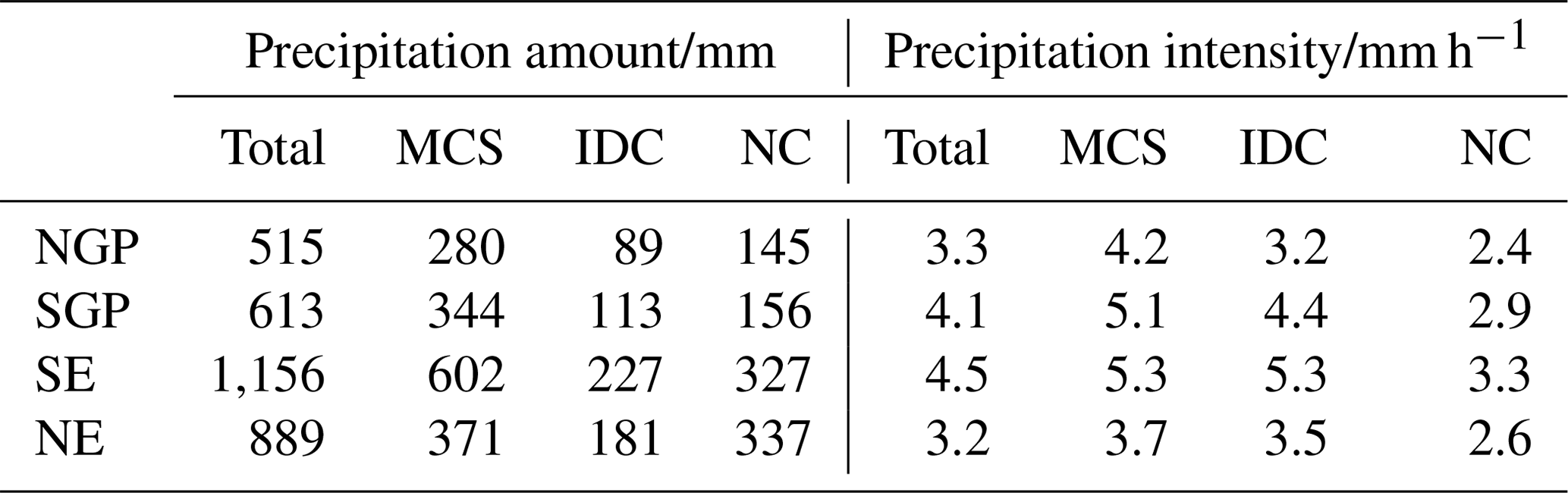
Table A7Annual mean seasonal precipitation amounts and intensities for different types of precipitation in different regions of the US for 2004–2017 by using the new MCS definition.
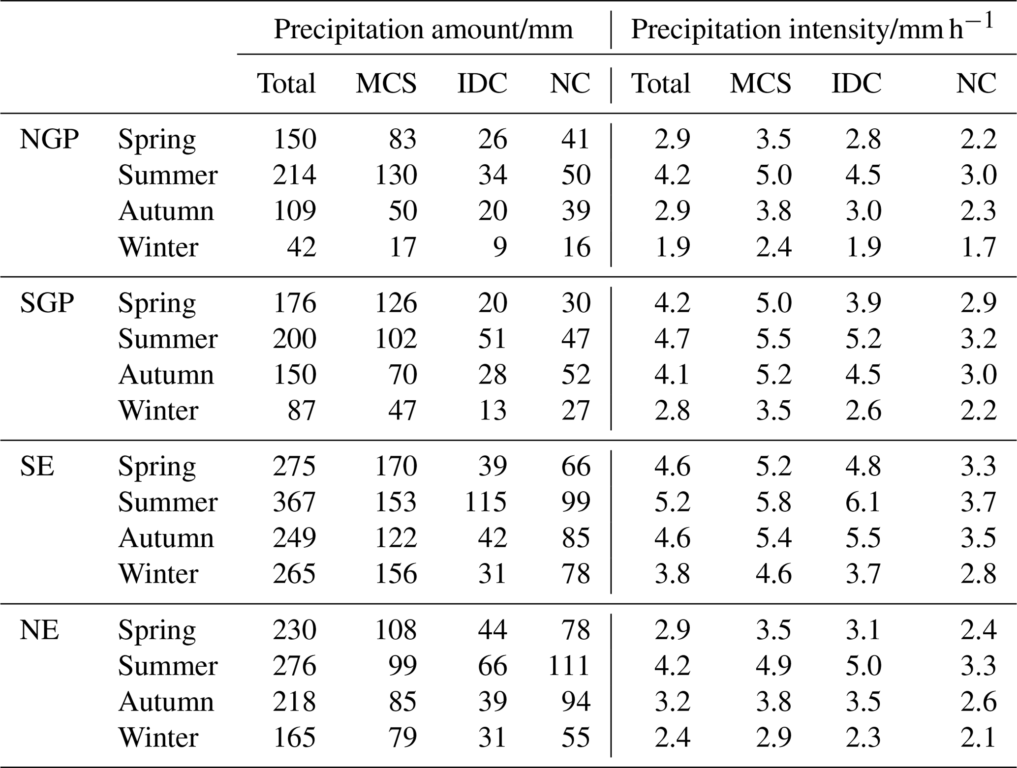
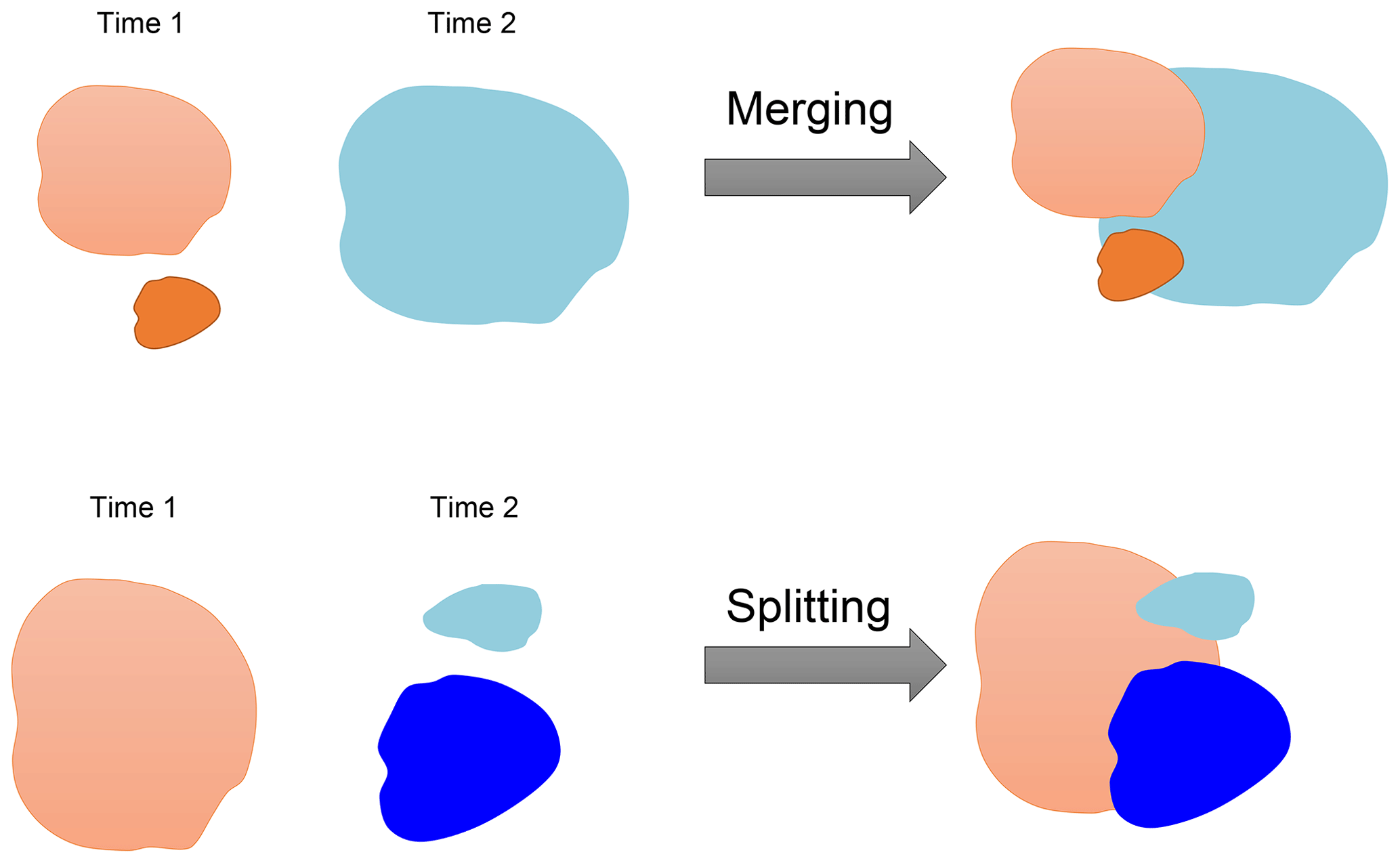
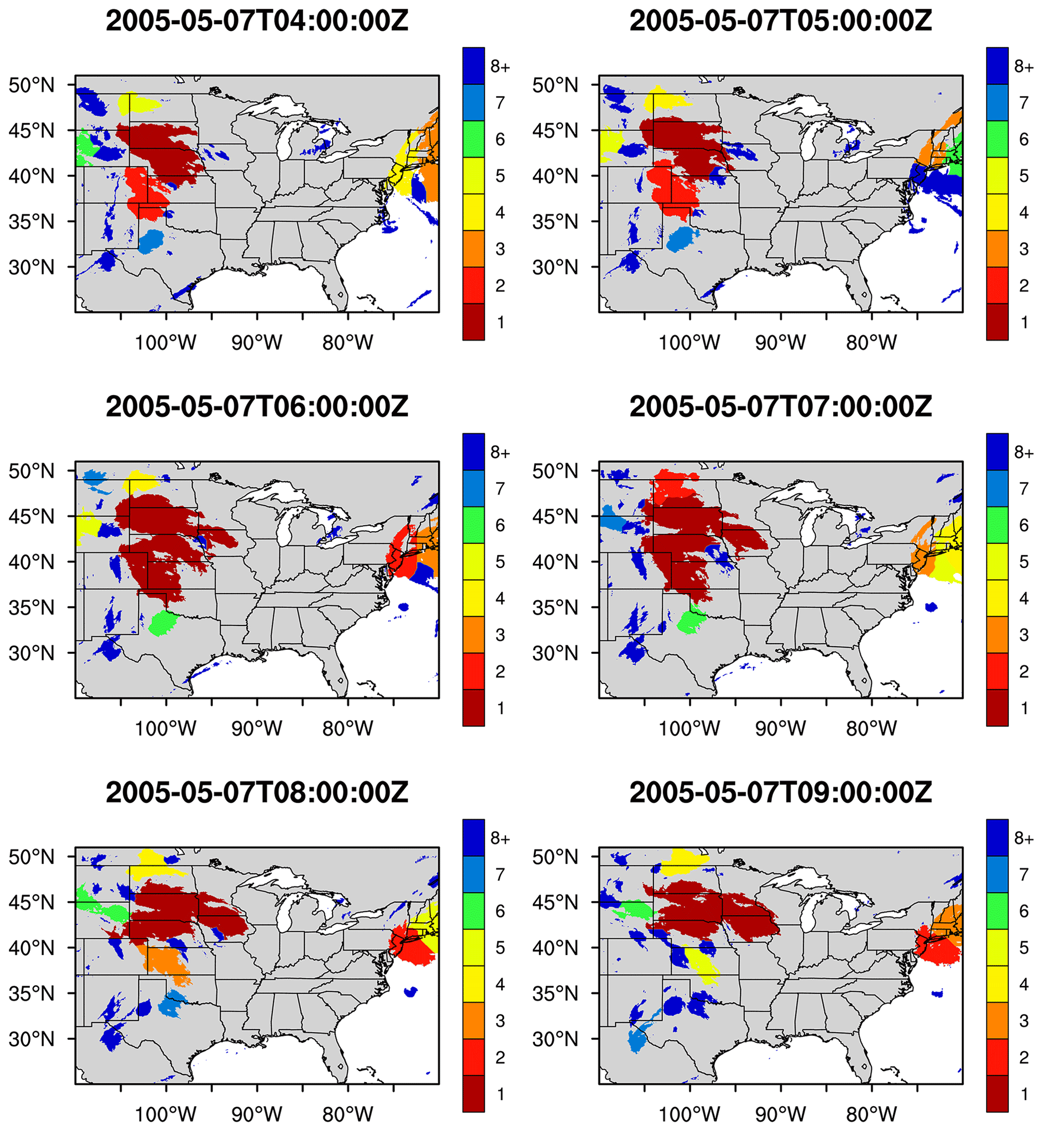
Figure A2An example of CCS merging and splitting from 2005-05-07T04:00:00 Z–T09:00:00 Z. Cloud 1 and Cloud 2 at 05:00:00 Z merged into Cloud 1 at 06:00:00 Z. And Cloud 1 at 7:00:00 Z at least split to Cloud 1 and Cloud 3 at 08:00:00 Z.
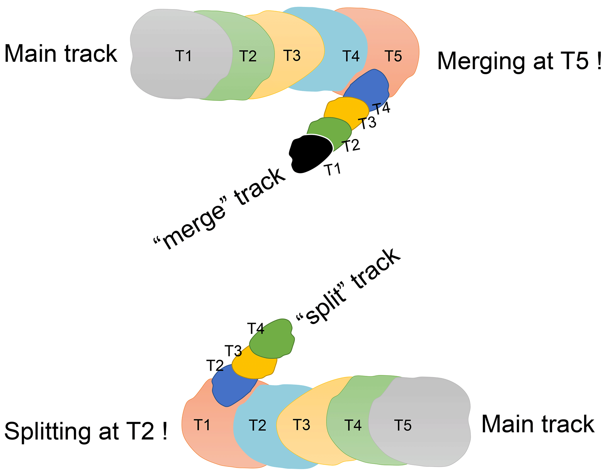
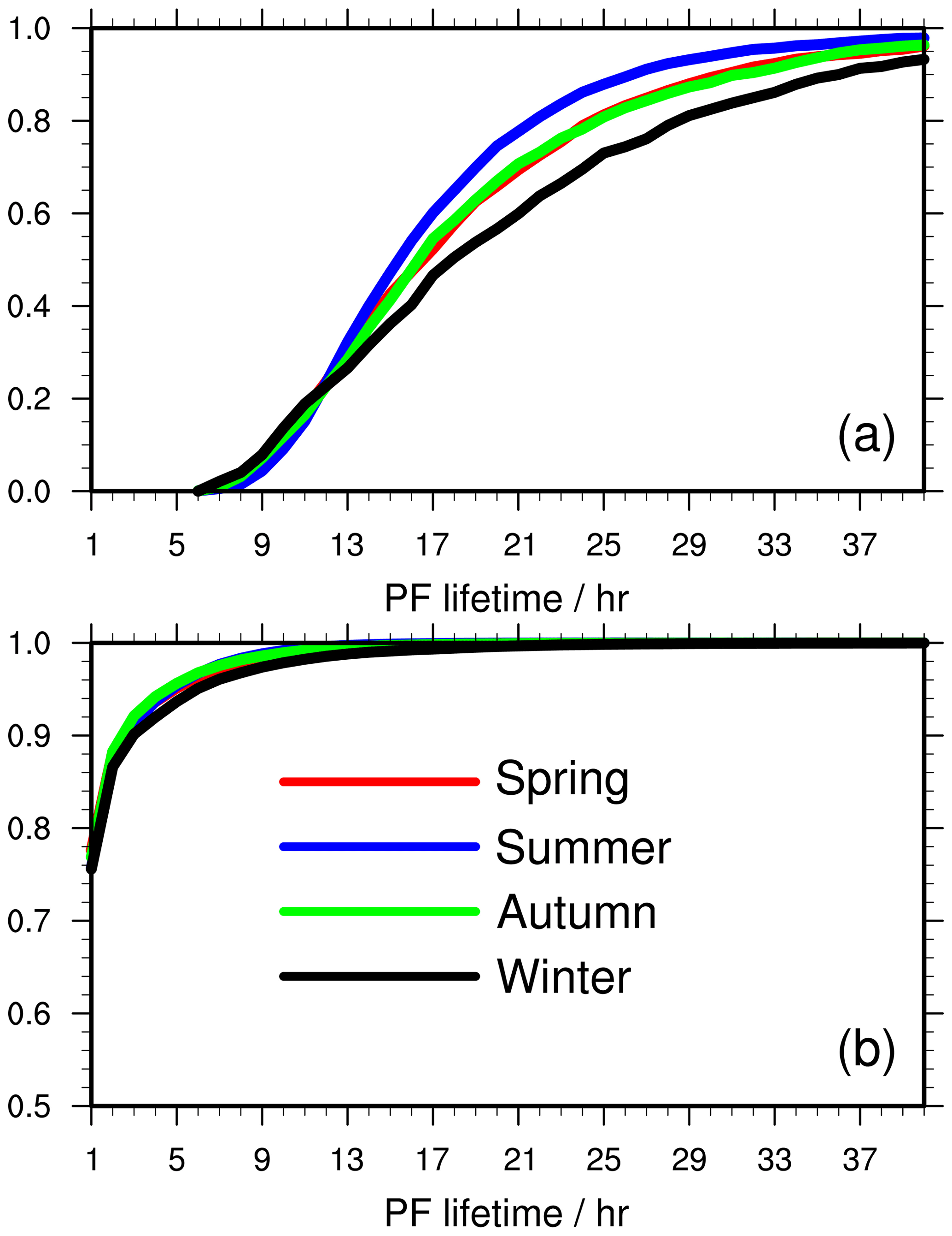
Figure A4Seasonal cumulative distribution functions of PF-based lifetimes for (a) MCSs and (b) IDC in the data product domain for 2004–2017. Red lines denote spring, blue lines denote summer, green lines denote autumn, and black lines denote winter.
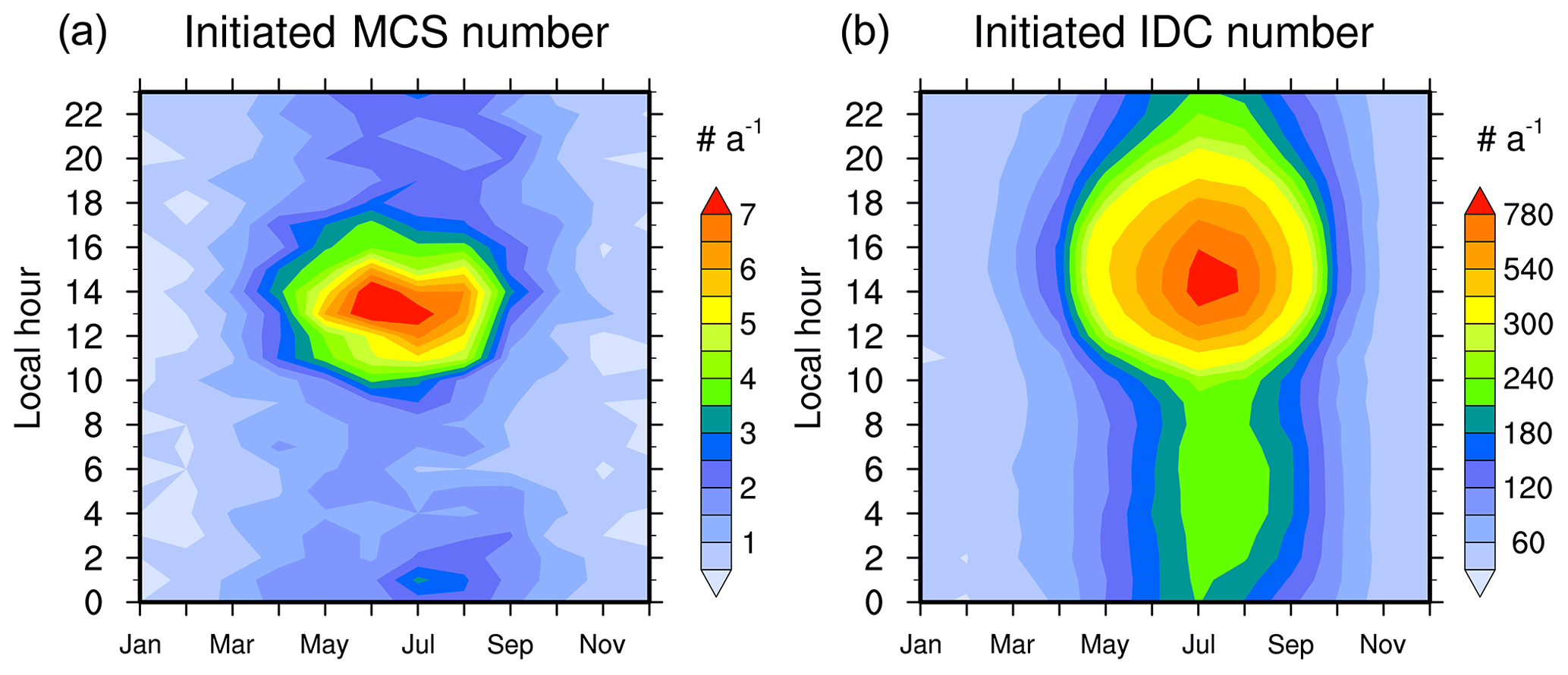
Figure A5Annual mean monthly diurnal cycles of initiated MCS (a) and IDC (b) numbers in the data product domain for 2004–2017. Here, we define that an MCS or IDC event initiates when the first PF appears. Therefore, we can derive the initiated time of all MCS and IDC events, which is the basis of this figure. For example, on average, more than seven MCSs initiated at 14:00 local time every June between 2004 and 2017.
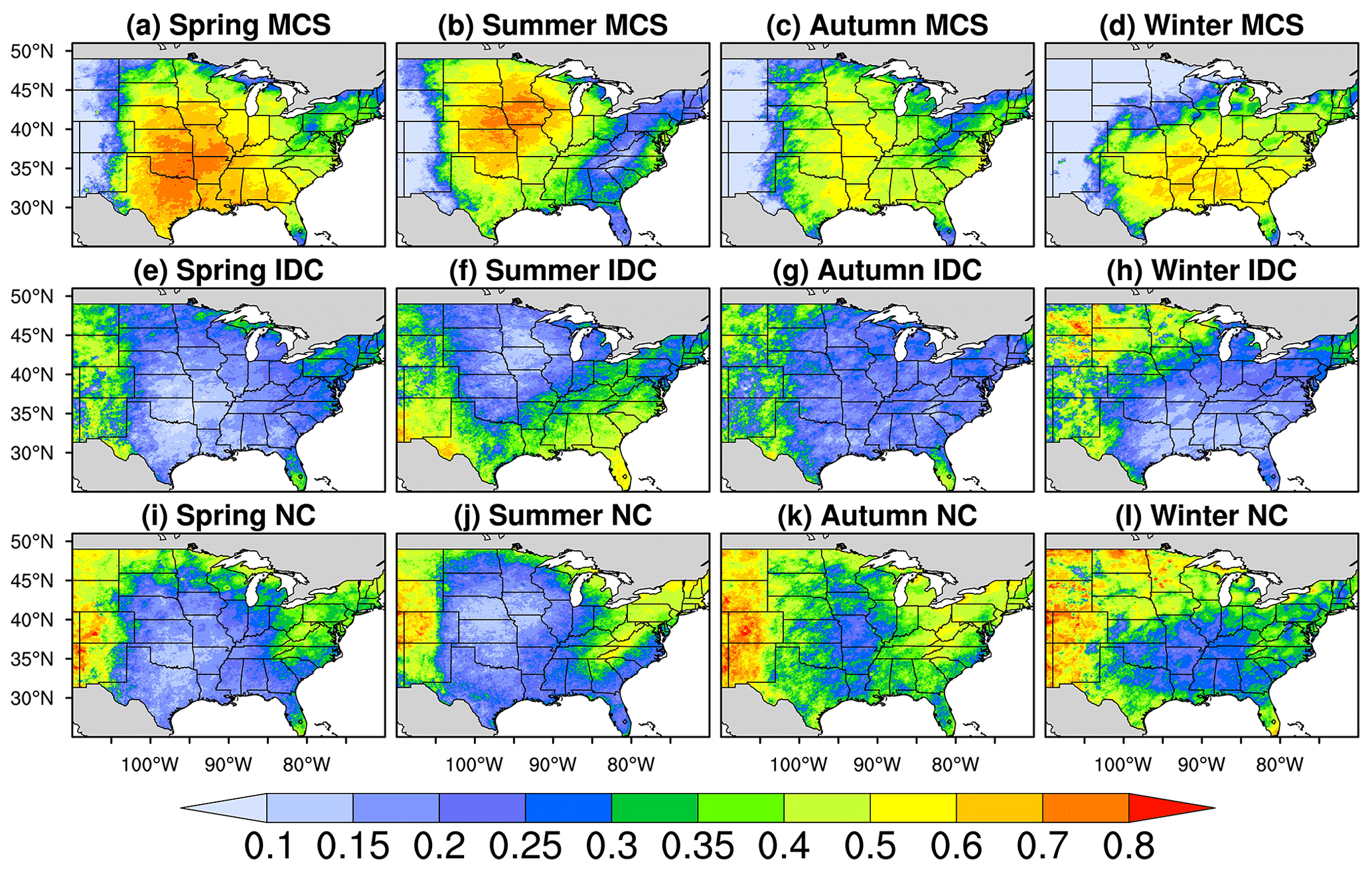
Figure A6Distributions of the fractions of different types of precipitation in each season. Here, precipitation refers to annual mean seasonal amounts for 2004–2017. We exclude hourly data with precipitation ≤ 1 mm h−1 in the calculation. The first row is for total precipitation, the second for MCS precipitation, the third for IDC precipitation, and the fourth for NC precipitation. The first column shows spring precipitation, the second summer, the third autumn, and the fourth winter.
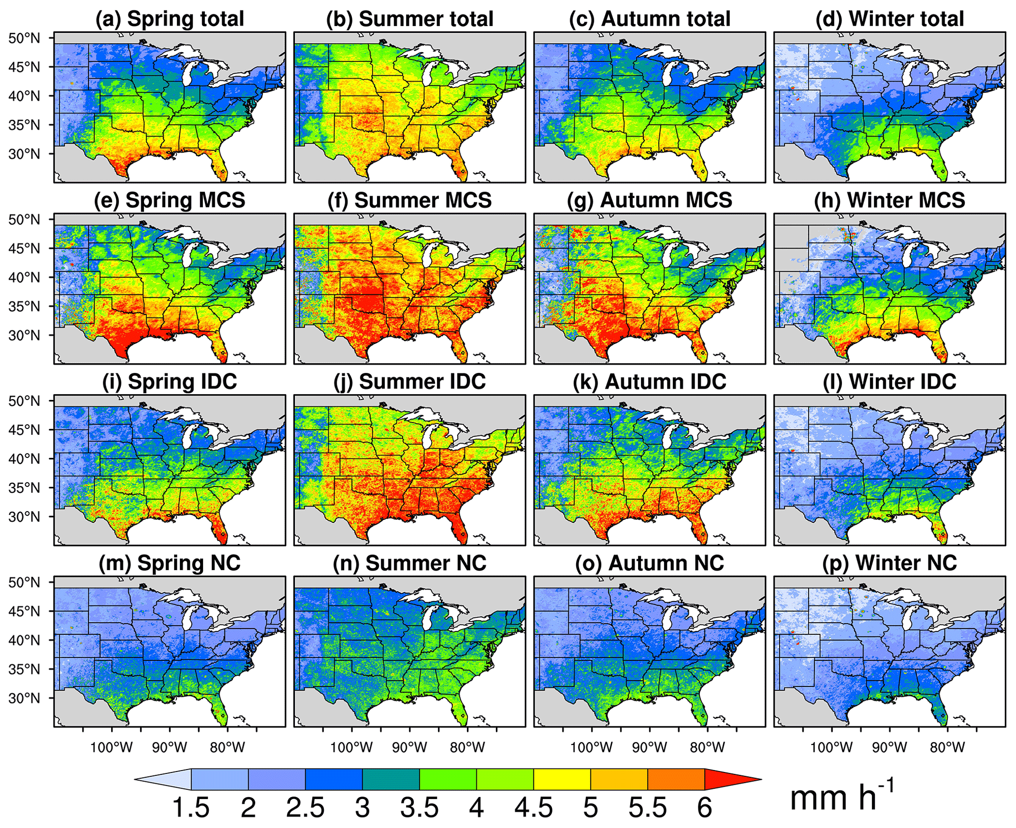
Figure A7Distributions of annual mean seasonal precipitation intensities for different types of precipitation for 2004–2017. The first row is for total precipitation, the second for MCS precipitation, the third for IDC precipitation, and the fourth for NC precipitation. The first column shows spring precipitation, the second summer, the third autumn, and the fourth winter. We exclude hourly data with precipitation ≤ 1 mm h−1 in the calculation.
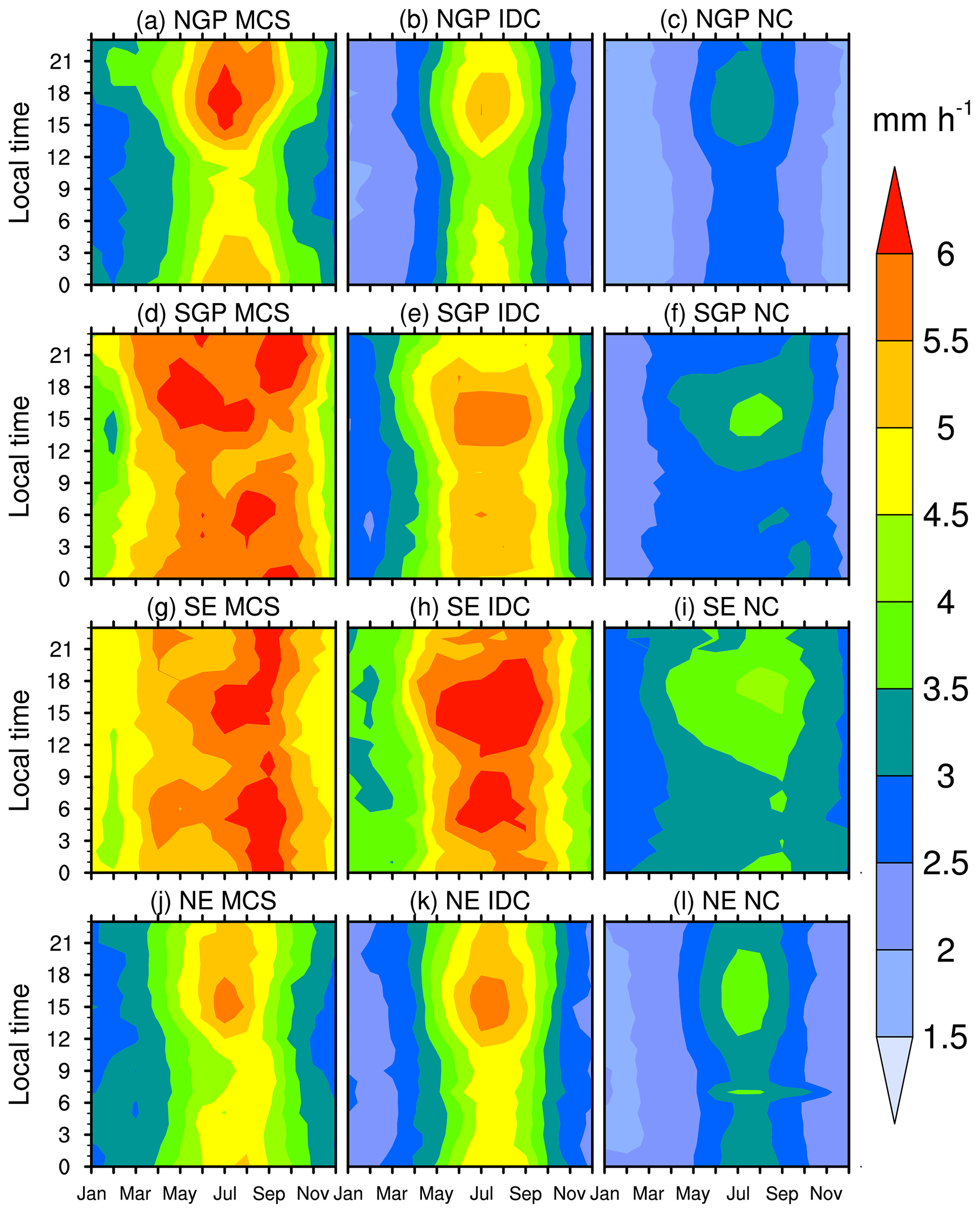
Figure A8Monthly mean diurnal cycles of precipitation intensities for MCSs (a, d, g, j), IDC (b, e, h, k), and NC (c, f, i, l) in the NGP (a, b, c), SGP (d, e, f), SE (g, h, i), and NE (j, k, l) during 2004–2017.
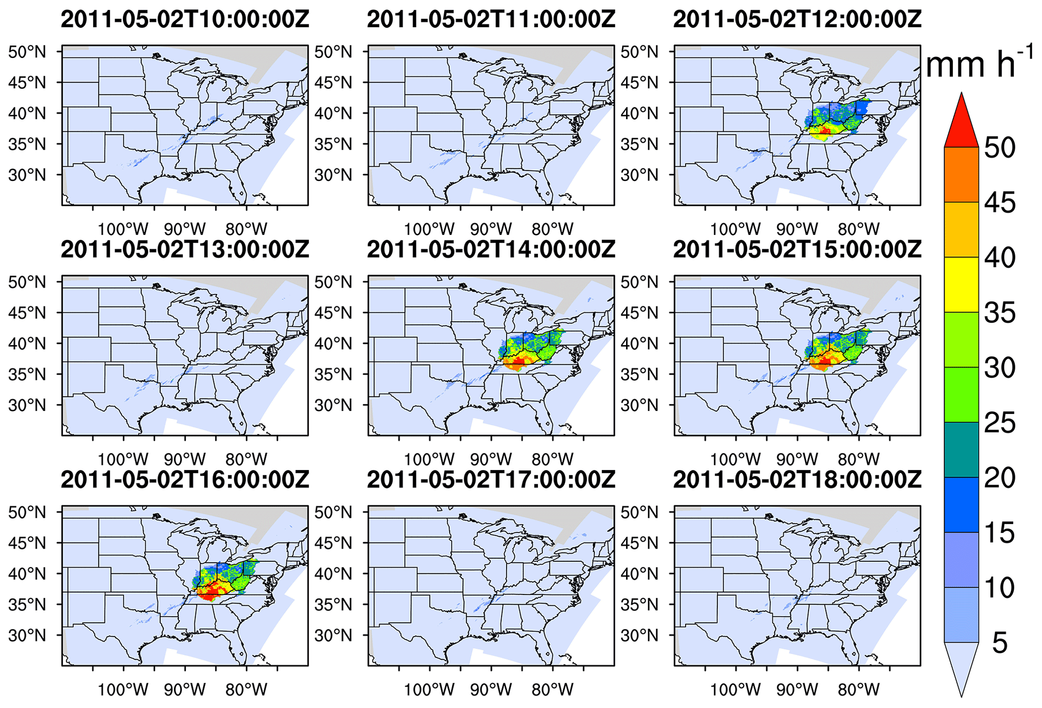
Figure A9An example of Stage IV erroneous precipitation. Stage IV shows a large area of intense precipitation suddenly appearing at 2011-05-02T12:00:00 Z, which then unexpectedly disappears at 13:00:00 Z, comes back abruptly at 14:00:00 Z, and finally goes away immediately at 17:00:00 Z.
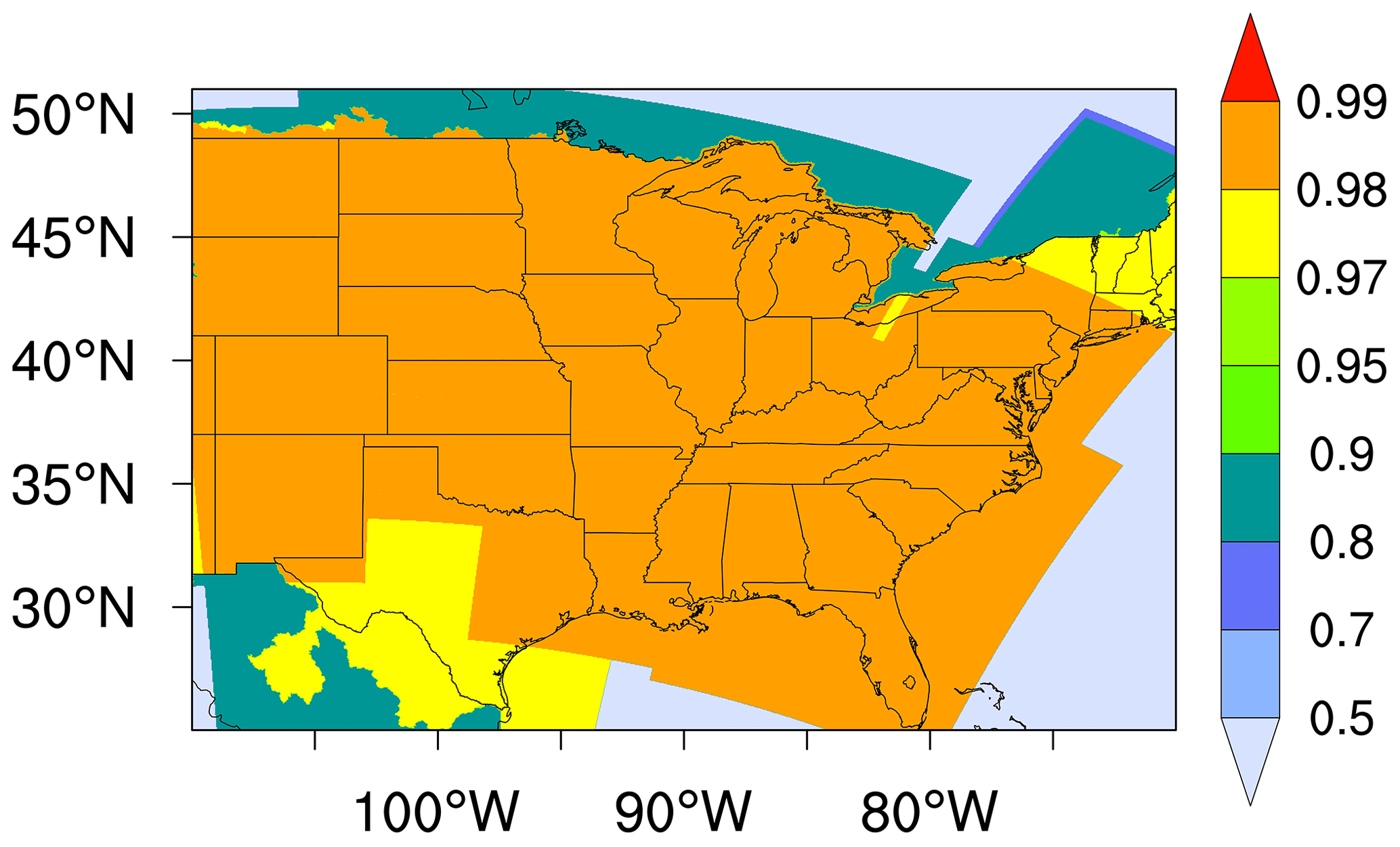
Figure A10Distribution of the fraction of valid Stage IV precipitation data for 2004–2017. Here, “valid” means that precipitation data are available and reasonable. The erroneous precipitation discussed in Sect. 4.1 is unreasonable and invalid.
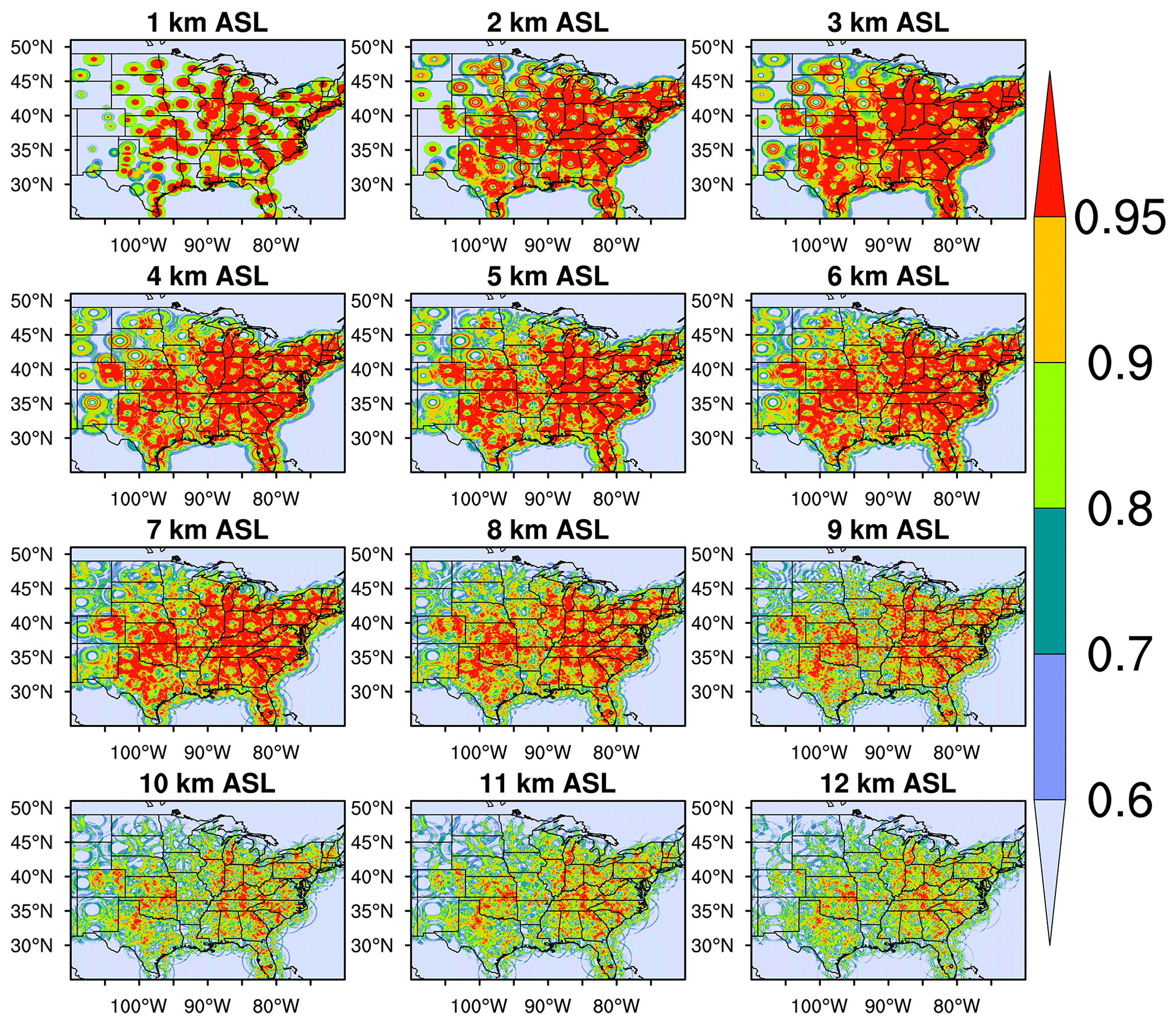
Figure A11Distributions of the fractions of available radar reflectivity data for 2004–2017 at different vertical levels. As long as radars scan a grid cell, we think of it as “available” even though there is no echo.
JL and ZF updated the FLEXTRKR algorithm and prepared the source datasets. JL ran the SL3D and updated FLEXTRKR algorithms for 2004–2017. JL collected and archived the MCS–IDC data product and did the analyses. JL led the writing of the manuscript with input from ZF, YQ, and LRL. YQ and LRL guided the development of the data product. JL, ZF, YQ, and LRL reviewed the manuscript.
The authors declare that they have no conflict of interest.
We thank Cameron R. Homeyer from the University of Oklahoma for helping us understand the GridRad dataset and Jingyu Wang from PNNL for identifying the existence of erroneous Stage IV precipitation. We obtain the NCEP/CPP L3 half-hourly 4 km Global Merged IR V1 brightness temperature dataset from https://disc.gsfc.nasa.gov/datasets/GPM_MERGIR_1/summary (last access: 28 December 2019, Janowiak et al., 2017). The 3D GridRad dataset is from https://rda.ucar.edu/datasets/ds841.0/ (last access: 2 January 2020, Bowman and Homeyer, 2017). We download hourly Stage IV precipitation data from https://rda.ucar.edu/datasets/ds507.5/ (last access: 28 December 2019, CODIAC et al., 2000), and the ERA5 melting level height data were downloaded from https://doi.org/10.24381/cds.adbb2d47 (last access: 24 January 2020, ECMWF, 2018).
This research has been supported by the U.S. Department of Energy Office of Science Biological and Environmental Research as part of the Regional and Global Modeling and Analysis (RGMA) program area through the collaborative, multi-program Integrated Coastal Modeling (ICoM) project. LRL and ZF have also been partly supported by the Water Cycle and Climate Extremes Modeling (WACCEM) Scientific Focus Area funded by RGMA. The research has used computational resources from the National Energy Research Scientific Computing Center (NERSC), a DOE User Facility supported by the Office of Science under contract DE-AC02-05CH11231. PNNL is operated for the DOE by the Battelle Memorial Institute under contract DE-AC05-76RL01830.
This paper was edited by David Carlson and reviewed by Rebecca Adams-Selin and Tomeu Rigo.
Anderson, J. G., Weisenstein, D. K., Bowman, K. P., Homeyer, C. R., Smith, J. B., Wilmouth, D. M., Sayres, D. S., Klobas, J. E., Leroy, S. S., and Dykema, J. A.: Stratospheric ozone over the United States in summer linked to observations of convection and temperature via chlorine and bromine catalysis, P. Natl. Acad. Sci. USA, 114, E4905–E4913, https://doi.org/10.1073/pnas.1619318114, 2017.
Andreae, M. O., Artaxo, P., Fischer, H., Freitas, S., Grégoire, J. M., Hansel, A., Hoor, P., Kormann, R., Krejci, R., and Lange, L.: Transport of biomass burning smoke to the upper troposphere by deep convection in the equatorial region, Geophys. Res. Lett., 28, 951–954, https://doi.org/10.1029/2000GL012391, 2001.
Angel, J. R., Palecki, M. A., and Hollinger, S. E.: Storm precipitation in the United States. Part II: Soil erosion characteristics, J. Appl. Meteorol., 44, 947–959, https://doi.org/10.1175/JAM2242.1, 2005.
Bigelbach, B., Mullendore, G., and Starzec, M.: Differences in deep convective transport characteristics between quasi-isolated strong convection and mesoscale convective systems using seasonal WRF simulations, J. Geophys. Res.-Atmos., 119, 11445–11455, https://doi.org/10.1002/2014JD021875, 2014.
Bowman, K. P. and Homeyer, C. R.: GridRad – Three-Dimensional Gridded NEXRAD WSR-88D Radar Data, Research Data Archive at the National Center for Atmospheric Research, Computational and Information Systems Laboratory, https://doi.org/10.5065/D6NK3CR7, available at: https://rda.ucar.edu/datasets/ds841.0/ (last access: 2 January 2020), 2017.
Brooks, H. E., Doswell III, C. A., and Kay, M. P.: Climatological estimatesof local daily tornado probability for the United States, Weather Forecast., 18, 626–640, https://doi.org/10.1175/1520-0434(2003)018<0626:CEOLDT>2.0.CO;2, 2003.
Carpenter, S. R., Booth, E. G., and Kucharik, C. J.: Extreme precipitation and phosphorus loads from two agricultural watersheds, Limnol. Oceanogr., 63, 1221–1233, https://doi.org/10.1002/lno.10767, 2018.
Changnon, S. A.: Damaging thunderstorm activity in the United States, B. Am. Meteorol. Soc., 82, 597–608, https://doi.org/10.1175/1520-0477(2001)082<0597:DTAITU>2.3.CO;2, 2001a.
Changnon, S. A.: Thunderstorm rainfall in the conterminous United States, B. Am. Meteorol. Soc., 82, 1925–1940, https://doi.org/10.1175/1520-0477(2001)082<1925:TRITCU>2.3.CO;2, 2001b.
Choi, S., Joiner, J., Choi, Y., Duncan, B. N., Vasilkov, A., Krotkov, N., and Bucsela, E.: First estimates of global free-tropospheric NO2 abundances derived using a cloud-slicing technique applied to satellite observations from the Aura Ozone Monitoring Instrument (OMI), Atmos. Chem. Phys., 14, 10565–10588, https://doi.org/10.5194/acp-14-10565-2014, 2014.
Cintineo, J. L., Pavolonis, M. J., Sieglaff, J. M., and Heidinger, A. K.: Evolution of severe and nonsevere convection inferred from GOES-derived cloud properties, J. Appl. Meteorol. Clim., 52, 2009–2023, https://doi.org/10.1175/JAMC-D-12-0330.1, 2013.
CODIAC (Cooperative Distributed Interactive Atmospheric Catalog System), EOL (Earth Observing Laboratory), NCAR (National Center for Atmospheric Research), UCAR (University Corporation for Atmospheric Research), CPC (Climate Prediction Center), NCEP (National Centers for Environmental Prediction), NWS (National Weather Service), NOAA (National Oceanic and Atmospheric Administration), and DOC (U.S. Department of Commerce): NCEP/CPC Four Kilometer Precipitation Set, Gauge and Radar, Research Data Archive at the National Center for Atmospheric Research, Computational and Information Systems Laboratory, https://doi.org/10.5065/D69Z93M3 available at: https://rda.ucar.edu/datasets/ds507.5/ (last access: 28 December 2019), 2000.
Davis, C., Brown, B., and Bullock, R.: Object-based verification of precipitation forecasts. Part I: Methodology and application to mesoscale rain areas, Mon. Weather Rev., 134, 1772–1784, https://doi.org/10.1175/MWR3145.1, 2006.
Davison, M.: Shallow/Deep Convection, available at: https://www.wpc.ncep.noaa.gov/international/training/deep/index.htm (last access: 9 April 2020), 1999.
Derbile, E. K. and Kasei, R. A.: Vulnerability of crop production to heavy precipitation in north-eastern Ghana, Int. J. Clim. Chang. Str., 4, 36–53, https://doi.org/10.1108/17568691211200209, 2012.
Diffenbaugh, N. S., Scherer, M., and Trapp, R. J.: Robust increases in severe thunderstorm environments in response to greenhouse forcing, P. Natl. Acad. Sci. USA, 110, 16361–16366, https://doi.org/10.1073/pnas.1307758110, 2013.
Doswell III, C. A., Brooks, H. E., and Maddox, R. A.: Flash flood forecasting: An ingredients-based methodology, Weather Forecast., 11, 560–581, https://doi.org/10.1175/1520-0434(1996)011<0560:FFFAIB>2.0.CO;2, 1996.
ECMWF: ERA5 hourly data on single levels from 1979 to present, available at: https://cds.climate.copernicus.eu/cdsapp#!/dataset/reanalysis-era5-single-levels?tab=overview, https://doi.org/10.24381/cds.adbb2d47 (last access: 24 January 2020), 2018.
Feng, Z., Dong, X., Xi, B., Schumacher, C., Minnis, P., and Khaiyer, M.: Top-of-atmosphere radiation budget of convective core/stratiform rain and anvil clouds from deep convective systems, J. Geophys. Res.-Atmos., 116, D23202, https://doi.org/10.1029/2011JD016451, 2011.
Feng, Z., Dong, X., Xi, B., McFarlane, S. A., Kennedy, A., Lin, B., and Minnis, P.: Life cycle of midlatitude deep convective systems in a Lagrangian framework, J. Geophys. Res.-Atmos., 117, D23201, https://doi.org/10.1029/2012JD018362, 2012.
Feng, Z., Leung, L. R., Houze Jr, R. A., Hagos, S., Hardin, J., Yang, Q., Han, B., and Fan, J.: Structure and evolution of mesoscale convective systems: Sensitivity to cloud microphysics in convection-permitting simulations over the United States, J. Adv. Model. Earth Sy., 10, 1470–1494, https://doi.org/10.1029/2018MS001305, 2018.
Feng, Z., Houze Jr, R. A., Leung, L. R., Song, F., Hardin, J. C., Wang, J., Gustafson Jr, W. I., and Homeyer, C. R.: Spatiotemporal characteristics and large-scale environments of mesoscale convective systems east of the Rocky Mountains, J. Climate, 32, 7303–7328, https://doi.org/10.1175/JCLI-D-19-0137.1, 2019.
Folger, P. and Reed, A.: Severe thunderstorms and tornadoes in the United States, Congressional Research Service, 26 pp., available at https://fas.org/sgp/crs/misc/R40097.pdf (last access: 31 March 2020), 2013.
French, A. J. and Parker, M. D.: The initiation and evolution of multiple modes of convection within a meso-alpha-scale region, Weather Forecast., 23, 1221–1252, https://doi.org/10.1175/2008WAF2222136.1, 2008.
Fritsch, J. M., Kane, R. J., and Chelius, C. R.: The contribution of mesoscale convective weather systems to the warm-season precipitation in the United States, J. Appl. Meteorol. Climatol., 25, 1333–1345, https://doi.org/10.1175/1520-0450(1986)025<1333:TCOMCW>2.0.CO;2, 1986.
Futyan, J. M. and Del Genio, A. D.: Deep convective system evolution over Africa and the tropical Atlantic, J. Climate, 20, 5041–5060, https://doi.org/10.1175/JCLI4297.1, 2007.
Geerts, B.: Mesoscale convective systems in the southeast United States during 1994–95: A survey, Weather Forecast., 13, 860–869, https://doi.org/10.1175/1520-0434(1998)013<0860:MCSITS>2.0.CO;2, 1998.
Geerts, B., Parsons, D., Ziegler, C. L., Weckwerth, T. M., Biggerstaff, M. I., Clark, R. D., Coniglio, M. C., Demoz, B. B., Ferrare, R. A., and Gallus Jr, W. A.: The 2015 plains elevated convection at night field project, B. Am. Meteorol. Soc., 98, 767–786, https://doi.org/10.1175/BAMS-D-15-00257.1, 2017.
Giangrande, S. E., Krause, J. M., and Ryzhkov, A. V.: Automatic designation of the melting layer with a polarimetric prototype of the WSR-88D radar, J. Appl. Meteorol. Clim., 47, 1354–1364, https://doi.org/10.1175/2007JAMC1634.1, 2008.
Gourley, J. J., Hong, Y., Flamig, Z. L., Wang, J., Vergara, H., and Anagnostou, E. N.: Hydrologic evaluation of rainfall estimates from radar, satellite, gauge, and combinations on Ft. Cobb basin, Oklahoma, J. Hydrometeorol., 12, 973–988, https://doi.org/10.1175/2011JHM1287.1, 2011.
Grewe, V.: Impact of climate variability on tropospheric ozone, Sci. Total Environ., 374, 167–181, https://doi.org/10.1016/j.scitotenv.2007.01.032, 2007.
Groisman, P. Y., Knight, R. W., Karl, T. R., Easterling, D. R., Sun, B., and Lawrimore, J. H.: Contemporary changes of the hydrological cycle over the contiguous United States: Trends derived from in situ observations, J. Hydrometeorol., 5, 64–85, https://doi.org/10.1175/1525-7541(2004)005<0064:CCOTHC>2.0.CO;2, 2004.
Haberlie, A. M. and Ashley, W. S.: A radar-based climatology of mesoscale convective systems in the United States, J. Climate, 32, 1591–1606, https://doi.org/10.1175/JCLI-D-18-0559.1, 2019.
Hersbach, H., Bell, B., Berrisford, P., Horányi, A., Sabater, J. M., Nicolas, J., Radu, R., Schepers, D., Simmons, A., and Soci, C.: Global reanalysis: goodbye ERA-Interim, hello ERA5, in: ECMWF Newsletter, 159, 17–24, https://doi.org/10.21957/vf291hehd7, 2019.
Hodges, K. I. and Thorncroft, C.: Distribution and statistics of African mesoscale convective weather systems based on the ISCCP Meteosat imagery, Mon. Weather Rev., 125, 2821–2837, https://doi.org/10.1175/1520-0493(1997)125<2821:DASOAM>2.0.CO;2, 1997.
Homeyer, C. R. and Bowman, K. P.: Algorithm Description Document for Version 3.1 of the Three-Dimensional Gridded NEXRAD WSR-88D Radar (GridRad) Dataset, 23 pp., available at: http://gridrad.org/pdf/GridRad-v3.1-Algorithm-Description.pdf (last access: 30 March 2020), 2017.
Houze Jr, R. A.: Mesoscale convective systems, Rev. Geophys., 42, RG4003, https://doi.org/10.1029/2004RG000150, 2004.
Houze Jr, R. A., Wang, J., Fan, J., Brodzik, S., and Feng, Z.: Extreme convective storms over high-latitude continental areas where maximum warming is occurring, Geophys. Res. Lett., 46, 4059–4065, https://doi.org/10.1029/2019GL082414, 2019.
Hu, H., Leung, L. R., and Feng, Z.: Observed Warm-Season Characteristics of MCS and Non-MCS Rainfall and Their Recent Changes in the Central United States, Geophys. Res. Lett., 47, e2019GL086783, https://doi.org/10.1029/2019GL086783, 2020.
Janowiak, J., Joyce, B., and Xie, P.: NCEP/CPC L3 half hourly 4 km global (60 S–60 N) merged IR V1, Goddard Earth Sciences Data and Information Services Center (GES DISC), https://doi.org/10.5067/P4HZB9N27EKU, available at: https://disc.gsfc.nasa.gov/datasets/GPM_MERGIR_1/summary (last access: 28 December 2019), 2017.
Janowiak, J. E., Joyce, R. J., and Yarosh, Y.: A real-time global half-hourly pixel-resolution infrared dataset and its applications, B. Am. Meteorol. Soc., 82, 205–218, https://doi.org/10.1175/1520-0477(2001)082<0205:ARTGHH>2.3.CO;2, 2001.
Kalinga, O. A., and Gan, T. Y.: Estimation of rainfall from infrared-microwave satellite data for basin-scale hydrologic modelling, Hydrol. Process., 24, 2068–2086, https://doi.org/10.1002/hyp.7626, 2010.
Koehler, T. L.: Cloud-to-Ground Lightning Flash Density and Thunderstorm Day Distributions over the Contiguous United States Derived from NLDN Measurements: 1993–2018, Mon. Weather Rev., 148, 313–332, https://doi.org/10.1175/MWR-D-19-0211.1, 2020.
Li, J., Feng, Z., Qian, Y., and Leung, L. R.: MCSs and IDC in the US for 2004–2017, available at: https://data.pnnl.gov/dataset/13218, last access: 18 June 2020.
Lin, Y. and Mitchell, K. E.: NCEP stage II/IV hourly precipitation analyses: Development and applications, in Preprints, 19th Conf. on Hydrology, American Meteorological Society, San Diego, CA, USA, 9–13 January 2005, Paper 1.2, available at: https://ams.confex.com/ams/pdfpapers/83847.pdf (last access: 30 March 2020), 2005.
Liu, C., Zipser, E. J., and Nesbitt, S. W.: Global distribution of tropical deep convection: Different perspectives from TRMM infrared and radar data, J. Climate, 20, 489–503, https://doi.org/10.1175/JCLI4023.1, 2007.
Lopez, P.: Direct 4D-Var assimilation of NCEP stage IV radar and gauge precipitation data at ECMWF, Mon. Weather Rev., 139, 2098–2116, https://doi.org/10.1175/2010MWR3565.1, 2011.
Machado, L., Rossow, W., Guedes, R., and Walker, A.: Life cycle variations of mesoscale convective systems over the Americas, Mon. Weather Rev., 126, 1630–1654, https://doi.org/10.1175/1520-0493(1998)126<1630:LCVOMC>2.0.CO;2, 1998.
Motew, M., Booth, E. G., Carpenter, S. R., Chen, X., and Kucharik, C. J.: The synergistic effect of manure supply and extreme precipitation on surface water quality, Environ. Res. Lett., 13, 044016, https://doi.org/10.1088/1748-9326/aaade6, 2018.
Nearing, M., Pruski, F., and O'neal, M.: Expected climate change impacts on soil erosion rates: a review, J. Soil Water Conserv., 59, 43–50, 2004.
Nelson, B. R., Prat, O. P., Seo, D.-J., and Habib, E.: Assessment and implications of NCEP Stage IV quantitative precipitation estimates for product intercomparisons, Weather Forecast., 31, 371–394, https://doi.org/10.1175/WAF-D-14-00112.1, 2016.
Piani, C., Durran, D., Alexander, M., and Holton, J.: A numerical study of three-dimensional gravity waves triggered by deep tropical convection and their role in the dynamics of the QBO, J. Atmos. Sci., 57, 3689–3702, https://doi.org/10.1175/1520-0469(2000)057< 3689:ANSOTD>2.0.CO;2, 2000.
Pinto, J. O., Grim, J. A., and Steiner, M.: Assessment of the High-Resolution Rapid Refresh model's ability to predict mesoscale convective systems using object-based evaluation, Weather Forecast., 30, 892–913, https://doi.org/10.1175/WAF-D-14-00118.1, 2015.
Prein, A. F., Liu, C., Ikeda, K., Bullock, R., Rasmussen, R. M., Holland, G. J., and Clark, M.: Simulating North American mesoscale convective systems with a convection-permitting climate model, Clim. Dynam., 55, 95–110, https://doi.org/10.1007/s00382-017-3993-2, 2017.
Rosenzweig, C., Tubiello, F. N., Goldberg, R., Mills, E., and Bloomfield, J.: Increased crop damage in the US from excess precipitation under climate change, Global Environ. Chang., 12, 197–202, https://doi.org/10.1016/S0959-3780(02)00008-0, 2002.
Rowe, A. K., Rutledge, S. A., and Lang, T. J.: Investigation of microphysical processes occurring in isolated convection during NAME, Mon. Weather Rev., 139, 424–443, https://doi.org/10.1175/2010MWR3494.1, 2011.
Rowe, A. K., Rutledge, S. A., and Lang, T. J.: Investigation of microphysical processes occurring in organized convection during NAME, Mon. Weather Rev., 140, 2168–2187, https://doi.org/10.1175/MWR-D-11-00124.1, 2012.
Seeley, J. T. and Romps, D. M.: The effect of global warming on severe thunderstorms in the United States, J. Climate, 28, 2443–2458, https://doi.org/10.1175/JCLI-D-14-00382.1, 2015.
Sieglaff, J. M., Hartung, D. C., Feltz, W. F., Cronce, L. M., and Lakshmanan, V.: A satellite-based convective cloud object tracking and multipurpose data fusion tool with application to developing convection, J. Atmos. Ocean. Tech., 30, 510–525, https://doi.org/10.1175/JTECH-D-12-00114.1, 2013.
Smalley, M., L'Ecuyer, T., Lebsock, M., and Haynes, J.: A comparison of precipitation occurrence from the NCEP Stage IV QPE product and the CloudSat Cloud Profiling Radar, J. Hydrometeorol., 15, 444–458, https://doi.org/10.1175/JHM-D-13-048.1, 2014.
Song, F., Feng, Z., Leung, L. R., Houze Jr, R. A., Wang, J., Hardin, J., and Homeyer, C. R.: Contrasting spring and summer large-scale environments associated with mesoscale convective systems over the US Great Plains, J. Climate, 32, 6749–6767, https://doi.org/10.1175/JCLI-D-18-0839.1, 2019.
Starzec, M., Homeyer, C. R., and Mullendore, G. L.: Storm labeling in three dimensions (SL3D): A volumetric radar echo and dual-polarization updraft classification algorithm, Mon. Weather Rev., 145, 1127–1145, https://doi.org/10.1175/MWR-D-16-0089.1, 2017.
Steiner, M., Houze Jr, R. A., and Yuter, S. E.: Climatological characterization of three-dimensional storm structure from operational radar and rain gauge data, J. Appl. Meteorol., 34, 1978–2007, https://doi.org/10.1175/1520-0450(1995)034<1978:CCOTDS>2.0.CO;2, 1995.
Stensrud, D. J.: Effects of persistent, midlatitude mesoscale regions of convection on the large-scale environment during the warm season, J. Atmos. Sci., 53, 3503–3527, https://doi.org/10.1175/1520-0469(1996)053<3503:EOPMMR>2.0.CO;2, 1996.
Stensrud, D. J.: Upscale effects of deep convection during the North American monsoon, J. Atmos. Sci., 70, 2681–2695, https://doi.org/10.1175/JAS-D-13-063.1, 2013.
Taszarek, M., Allen, J. T., Púèik, T., Hoogewind, K. A., and Brooks, H. E.: Severe convective storms across Europe and the United States. Part II: ERA5 environments associated with lightning, large hail, severe wind, and tornadoes, J. Climate, 33, 10263–10286, https://doi.org/10.1175/JCLI-D-20-0346.1, 2020.
Thompson, A. M., Tao, W.-K., Pickering, K. E., Scala, J. R., and Simpson, J.: Tropical deep convection and ozone formation, B. Am. Meteorol. Soc., 78, 1043–1054, https://doi.org/10.1175/1520-0477(1997)078<1043:TDCAOF>2.0.CO;2, 1997.
Tian, B., Held, I. M., Lau, N. C., and Soden, B. J.: Diurnal cycle of summertime deep convection over North America: A satellite perspective, J. Geophys. Res.-Atmos., 110, D08108, https://doi.org/10.1029/2004JD005275, 2005.
Tippett, M. K., Allen, J. T., Gensini, V. A., and Brooks, H. E.: Climate and hazardous convective weather, Curr. Clim. Chang. Rep., 1, 60–73, https://doi.org/10.1007/s40641-015-0006-6, 2015.
Twohy, C. H., Clement, C. F., Gandrud, B. W., Weinheimer, A. J., Campos, T. L., Baumgardner, D., Brune, W. H., Faloona, I., Sachse, G. W., and Vay, S. A.: Deep convection as a source of new particles in the midlatitude upper troposphere, J. Geophys. Res.-Atmos., 107, AAC 6-1–AAC 6–10, https://doi.org/10.1029/2001JD000323, 2002.
Walker, J. R., MacKenzie Jr, W. M., Mecikalski, J. R., and Jewett, C. P.: An enhanced geostationary satellite–based convective initiation algorithm for 0–2-h nowcasting with object tracking, J. Appl. Meteorol. Clim., 51, 1931–1949, https://doi.org/10.1175/JAMC-D-11-0246.1, 2012.
Wang, P. K.: Moisture plumes above thunderstorm anvils and their contributions to cross-tropopause transport of water vapor in midlatitudes, J. Geophys. Res.-Atmos., 108, 4194, https://doi.org/10.1029/2002JD002581, 2003.
Yang, Q., Houze Jr, R. A., Leung, L. R., and Feng, Z.: Environments of long-lived mesoscale convective systems over the central United States in convection permitting climate simulations, J. Geophys. Res.-Atmos., 122, 13288–13307, https://doi.org/10.1002/2017JD027033, 2017.
Yuan, H., McGinley, J. A., Schultz, P. J., Anderson, C. J., and Lu, C.: Short-range precipitation forecasts from time-lagged multimodel ensembles during the HMT-West-2006 campaign, J. Hydrometeorol., 9, 477–491, https://doi.org/10.1175/2007JHM879.1, 2008.
Zhang, K., Randel, W. J., and Fu, R.: Relationships between outgoing longwave radiation and diabatic heating in reanalyses, Clim. Dynam., 49, 2911–2929, https://doi.org/10.1007/s00382-016-3501-0, 2017.