the Creative Commons Attribution 4.0 License.
the Creative Commons Attribution 4.0 License.
 | 03 Mar 2021
Homogenization of the historical series from the Coimbra Magnetic Observatory, Portugal
Anna L. Morozova
Paulo Ribeiro
M. Alexandra Pais
The Coimbra Magnetic Observatory (COI), Portugal, established in 1866, has provided nearly continuous records of the geomagnetic field elements for more than 150 years. However, during its long lifetime inevitable changes to the instruments and measurement procedures and even the relocation of the observatory have taken place. In our previous work (Morozova et al., 2014) we performed homogenization – elimination of the artificial changes – of the measured declination series (D) for the period from 1866 to 2006. In this paper we continue work on applying homogenization procedures to the measured series of the absolute monthly values of the horizontal (H, 1866–2006), vertical (Z, 1951–2006) and inclination components (I, 1866–1941). After homogenization of all measured series for the 1866–2006 time interval, we performed the homogenization of the series of all geomagnetic field elements (X, Y, Z, H, D, I and F) to the level of the 2015 epoch. Since all series except D have a gap of about 10 years in the middle of the 20th century, splitting each of them into two, the homogenization to the level of 2015 was done only for the series available after 1951 (with the D series homogenized for the whole time interval of 1866–2015). The COI geomagnetic field elements are available via the following addresses: https://doi.org/10.5281/zenodo.4308022 (Ribeiro et al., 2020) for the original COI data (ASCII and XLSX formats) and https://doi.org/10.5281/zenodo.4308036 (Morozova et al., 2020) for the homogenized COI data (ASCII and XLSX formats).
- Article
(11110 KB) - Full-text XML
-
Supplement
(2777 KB) - BibTeX
- EndNote


In previous work by Morozova et al. (2014), the series of monthly values of the declination of the geomagnetic field (D) measured at the Coimbra Magnetic Observatory (COI) between 1866 and 2006 were analyzed for the presence of artificial homogeneity breaks (HBs). A number of HBs related to the changes to the observatory location and instrument changes or repairs were found and, when possible, corrected. Here we present the continuation of the previous work, extending the homogeneity analysis to the monthly series of the horizontal (H) and vertical (Z) components and the inclination (I) measured at COI between 1866 and 2006. In 2006 the set of old instruments was replaced with modern instruments, which are still in use. Accordingly, we applied the same methods to the series of all elements for the 2006–2015 time interval to bring them in line with current measurements done with instruments installed after 2006. At the time of the analysis, the most recent values in the series were available for December 2015. Because from that time on no changes to the instruments and procedures have taken place, the addition of the corrected series of measurements done after December 2015 will not affect their homogeneity.
The analysis is supported by metadata about the instruments used to measure the H, Z and I components between 1866 and 2015. More details about the history of the Coimbra Magnetic Observatory and metadata can be also found in Pais and Miranda (1995) and Morozova et al. (2014).
The first geomagnetic measurements at the Coimbra Magnetic Observatory were started in June 1866 at the Cumeada site (40∘12.4′ N, 8∘25.4′ W, 140 m a.s.l.). In January 1932 the observatory was relocated to a new site, Alto da Baleia (40∘13′ N, 8∘25.3′ W, 99 m a.s.l.), where it is still operating. The records have gaps that start between 1939 and 1942 (depending on the element) and end in October 1951. A number of instrument replacements and repairs, as well as changes to the measurement and calculation procedures, took place between 1866 and 2015. Those related to the measurements of H, Z and I are described below and summarized in Tables 1 (H), 2 (I) and 3 (Z). The information on the D component can be found in Morozova et al. (2014) and is also summarized in Table S1 in the Supplement.
Table 1Metadata for the H data set at the Cumeada and the Alto da Baleia sites: dates of the instrument replacements, relocations, changes to the measurement and calculation procedures, etc. Estimated corrections (δ) for the COI series for different time intervals are in the third column.

Table 2Metadata for the I data set at the Cumeada and the Alto da Baleia sites: dates of the instrument replacements, relocations, changes to the measurement and calculation procedures, etc. Estimated corrections (δ) for the COI series for different time intervals are in the third column. “d.n.u.” – it is not recommended to use the data for this time interval.
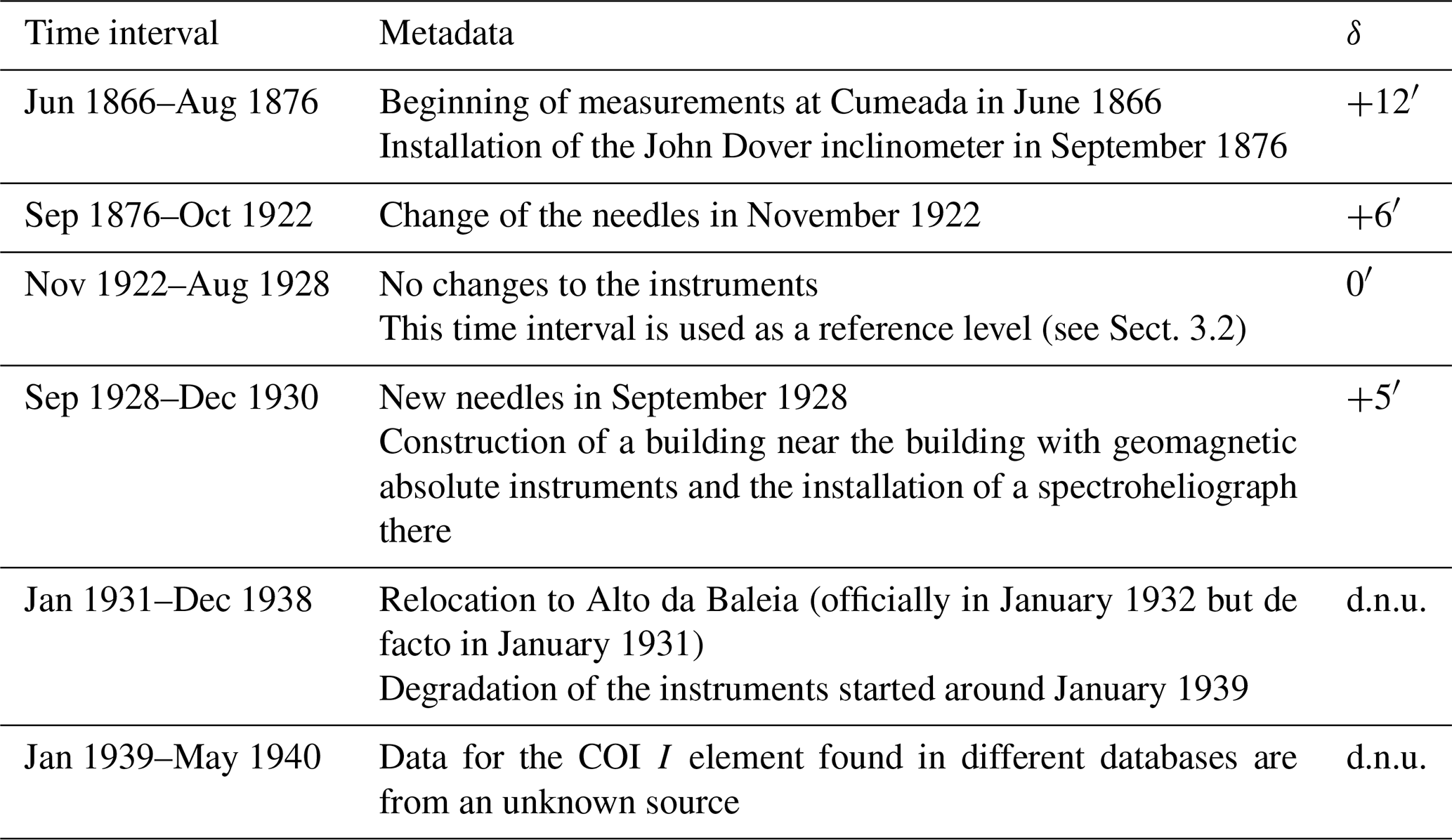
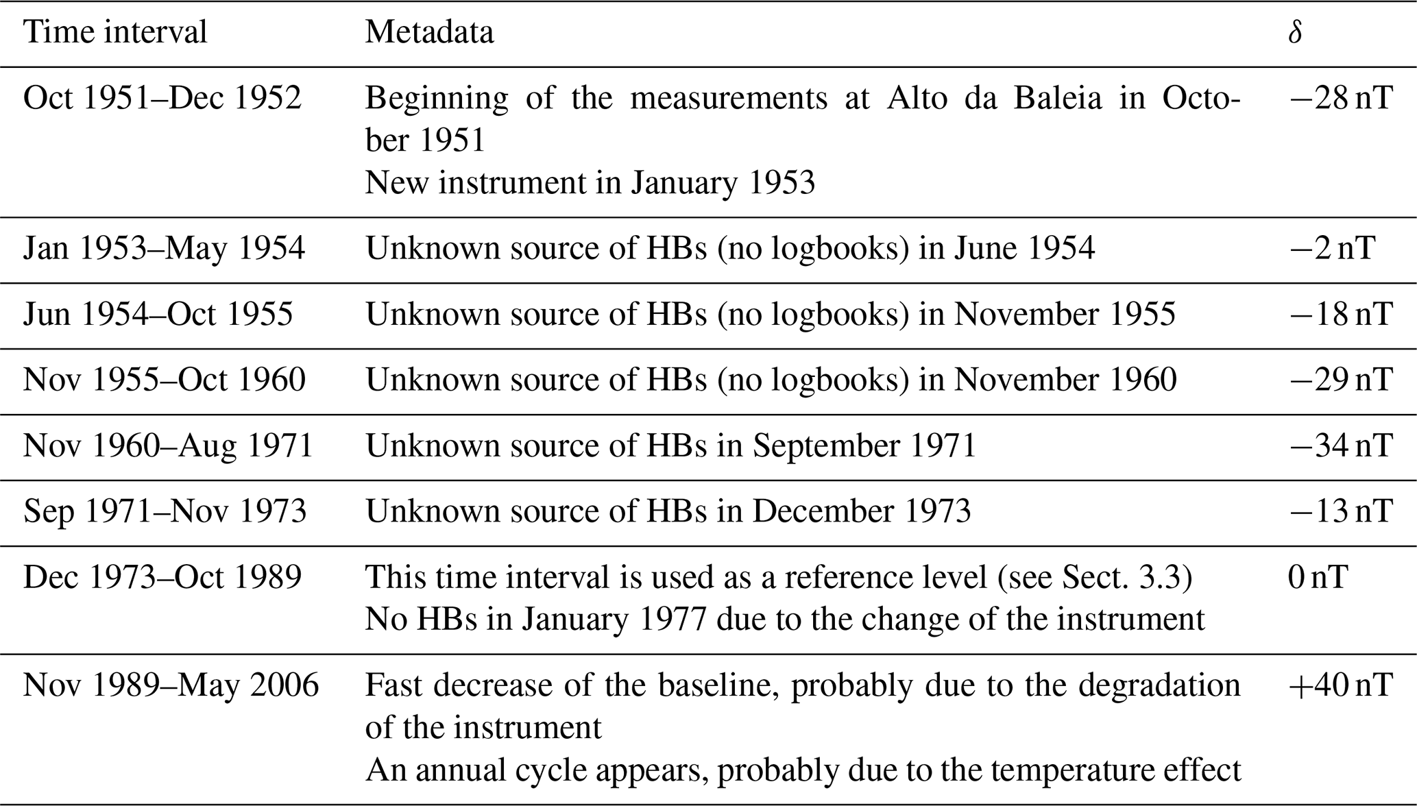
Table 3Metadata for the Z data set at the Alto da Baleia site: dates of the instrument replacements, relocations, changes to the measurement and calculation procedures, etc. Estimated corrections (δ) for the COI series for different time intervals are in the third column.
Different combinations of three magnetic elements can be used to fully specify the geomagnetic field vector. The particular combination is determined by the kind of instruments being used. The combinations of HDZ (cylindrical components) and XYZ (Cartesian) are commonly recorded by the relative instruments (i.e., variographs or variometers), while the combinations HDZ, HDI and DIF (spherical) are the most easily measured by absolute instruments (Parkinson, 1983). Table S1 in the Supplement shows the combinations of geomagnetic elements measured by the absolute and relative instruments in the Coimbra Magnetic Observatory from 1866 to 2015.
Concerning the absolute measurements, three different combinations of magnetic elements were registered in different periods of the observatory history. In the first period, between 1864 and 1951, the absolute observations were made for H, D and I. The Gibson unifilar magnetometer used in the first absolute observations of H and D was replaced in January 1878 with the Elliott Bros. unifilar magnetometer, which was kept running until 1948. The magnetic inclination (I) started to be measured with a Barrow inclinometer in June 1866, which later was replaced by a John Dover inclinometer in September 1876, which, in turn, was replaced by a Sartorius earth inductor in October 1935. The absolute measurements of I were discontinued in 1939. Despite the observatory relocation in 1932 to Alto da Baleia, relatively far from the city center and the tram lines, the quality of data did not improve and even deteriorated significantly during the first 20 years in Alto da Baleia (1932–1951). The oversimplification of observation routines and the non-negligible perturbations mainly related to the aging and drift of old absolute instruments that were kept in use, as well as the incorrect installation of the newly acquired Askania variographs, can be regarded as the main reasons for the low quality of the data. In the following period, between 1951–1952 and 2006, the absolute measurement of I was replaced by the measurement of Z so that the calculation of the baselines for the magnetic variations (H, D and Z) was now obtained directly from the absolute measurements of these elements (see Table S2).
After 1951 the absolute measurements of H and Z were obtained, respectively, with quartz horizontal magnetometers (QHMs) and zero-balance magnetometers (BMZs). The QHM and BMZ magnetometers are known to be semi-absolute instruments (i.e., instruments subject to drift) being then necessary to periodically assess the measurement quality by comparing them with standard instruments. Such comparisons were done in October 1951–October 1952 and in November and December 1952. In January 1953 one of the QHMs was adopted as the main observation instrument until 1955 when it was replaced by a new QHM. The comparison of the new and the old instruments showed consistent measurements, and the new QHM was used as the main instrument for absolute measurements of the horizontal component from beginning of July 1955 until May 2006.
The absolute measurement of the Z component at the Alto da Baleia site started in December 1951–January 1952, and the instruments were upgraded in January 1953 and in January 1977. Absolute determination of the vertical component was done until May 2006.
The installation of the current set of modern instruments at the Coimbra Magnetic Observatory took place during 2006–2007. It began in 2006, with the DI-flux for the absolute observations. This change resulted in a D baseline jump (Morozova et al., 2014).
The baselines of components H and Z continued to be determined using the absolute values obtained by the QHM and BMZ magnetometers until the end of May 2006. These two instruments were replaced in June 2006, and the baselines of H and Z started being computed through the absolute observations of D, I and F, obtained with the DI-flux (D and I) and the proton magnetometer (F). These equipment changes introduced discontinuities in the baselines of the H and Z series. In the case of H, there was a jump of −34 nT (considering the difference between values of June and May). In the case of component Z, there were two discontinuities: the first, also related to the change in the equipment of absolute measurements, resulted in a jump of −24 nT (considering the difference between the values of June and May), while the second, characterized by a jump of −25 nT (considering the difference between the August and September values), was related to the replacement of the analog variometers (Eschenhagen model) by a reliable and very stable fluxgate magnetometer model FGE, with a digital recording system. In May 2007, the proton sensor, initially installed at a height of about 2 m near the entrance of the pavilion of absolute measurements, was moved to the top of pillar no. 5. Later, in July 2007, the old proton magnetometer was replaced by the new one. This last modification apparently did not introduce significant discontinuities in the evolution of baselines. In addition, during most of the year 2014 it was not possible to carry out the absolute observations due to the failure of both the DI-flux (between February and September) and the proton magnetometer (between May and September). Both instruments were repaired by the respective companies (Bartington and GEM systems). During the period of interruption of the absolute observations the baselines calculated for January 2014 were used.
The full list of the instruments used at COI for the absolute measurements can be found in Table S3 in the Supplement.
The homogenization procedure used in this study is similar to the one described in detail in Morozova et al. (2014). It resorts to both the visual analysis and a statistical homogeneity test, namely the standard normal homogeneity test (SNHT, see Alexandersson and Moberg, 1997), which allows for the estimation of the statistical significance of homogeneity breaks (HBs). The SNHT is known to be oversensitive to HBs near the beginning and/or the end of the analyzed series (Costa and Soares, 2009). In general, the relative amplitude of a maximum of the SNHT statistics does not directly depend on the strength of the corresponding HB. The ratio of amplitudes of different maxima depends on the length of the studied period and relative distance between the breaks and/or to the proximity to the beginning or end of the series. Also, the correction of a break can result in changes of the relative amplitudes of other SNHT statistics' maxima. The natural cyclic variations and long-term trends of the measured parameters are also detected by the statistical homogeneity tests and have to be accounted for.
Contrary to Morozova et al. (2014), we found that to take care of all significant artificial homogeneity breaks we have to analyze not only the time derivatives of the geomagnetic series but the series themselves. In some cases abrupt changes in a series mean level are clearly seen in the visual analysis of a geomagnetic element but not in the homogeneity test of its time derivative (e.g., the change of the mean level of the H component in March 1922 discussed in Sect. 3.1), most probably shadowed by more significant inhomogeneities in the series.
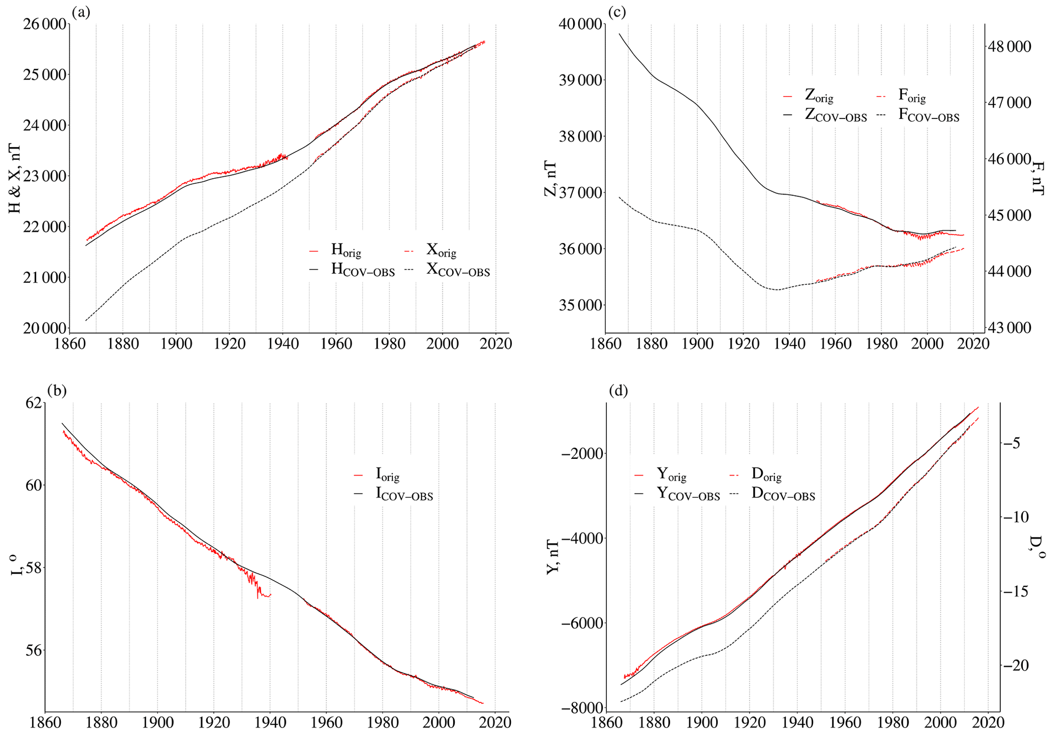
Figure 1For the 1866–2015 time period, measured series (red; orig) of the COI geomagnetic field elements and COV-OBS model predictions (black) of (a) H and X, (b) I, (c) F and Z, and (d) D and Y.
The data series of geomagnetic elements and their time derivatives were analyzed using relative homogeneity tests applied to differences between COI series and similar data obtained from other geomagnetic observatories or simulated by a model which we refer to as “reference series”. The series of these differences are denoted by adding the prefix “Δ”. The series of time derivatives were calculated as differences between the same months of 2 consecutive years. Since this time derivative is close to the standard geomagnetic secular variation, we will denote it “SV”. The original series of the analyzed components are shown in Fig. 1 as red lines. The SV series are shown in the Supplement (Fig. S1, red lines).
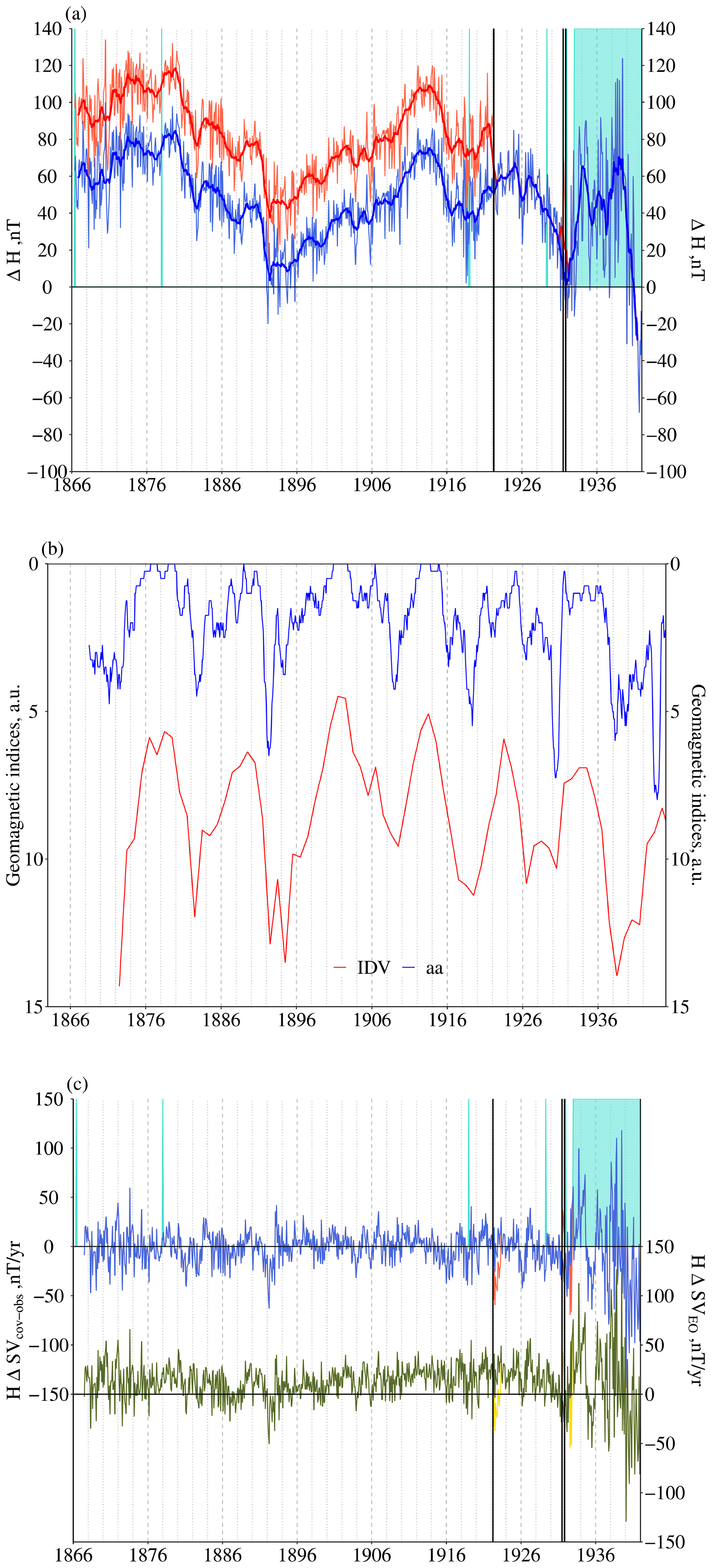
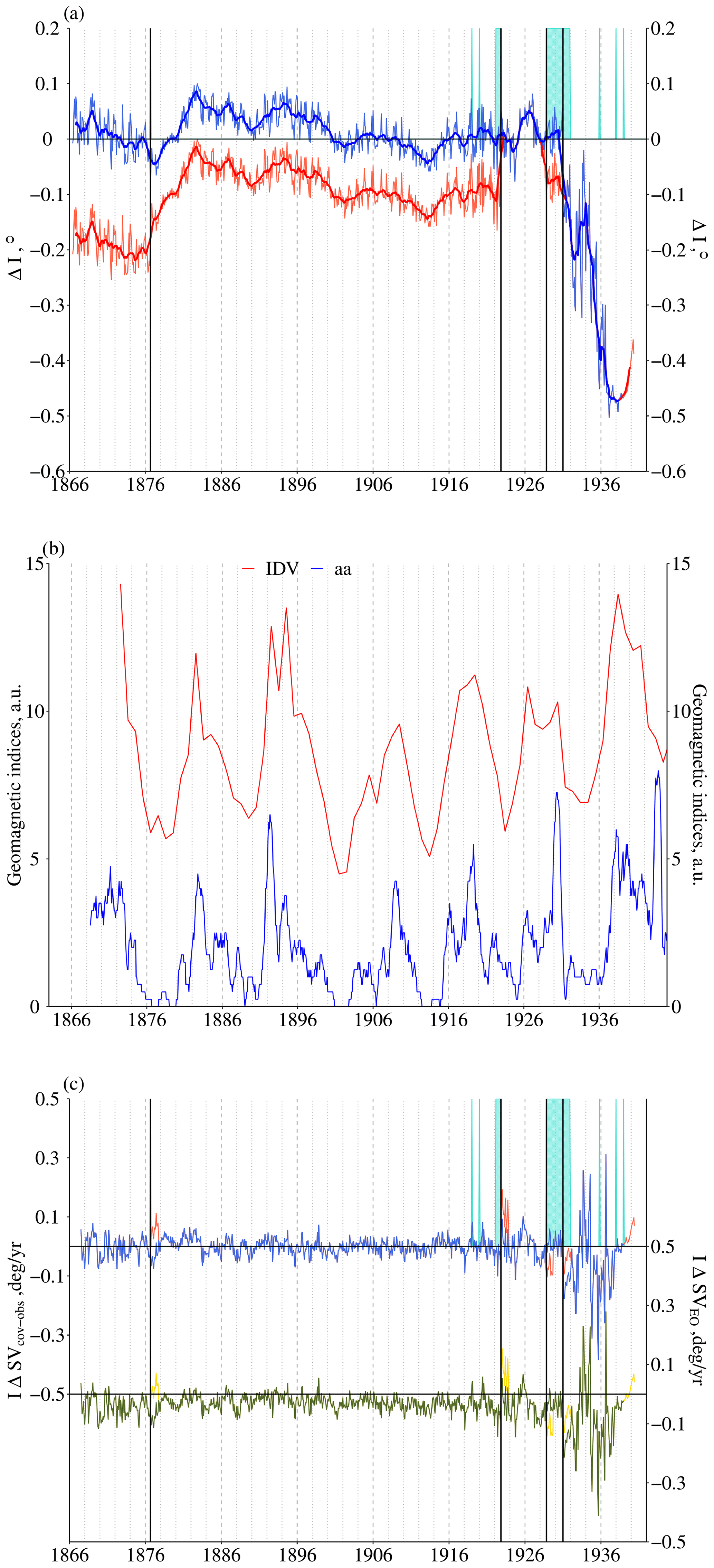
Figure 2(a) Original (red) and corrected (blue) COI ΔH series for the C–AdB (Cumeada and Alto da Baleia) period of measurements: 1866–1941. Thin lines are data, and thick lines are the moving average with a 12-month window. (b) Variations of the geomagnetic indices aa (monthly data, blue) and IDV (annual data, red). Please note the reversed y axis. (c) Original (red) and corrected (blue) ΔSVCOV−OBS series for H; original (yellow) and corrected (green) ΔSVEO series for H. Cyan vertical lines and rectangles mark possible HBs which are not corrected (see details in the text); black vertical lines mark dates of the corrected HBs.
Three types of series were used as references. The first type is observations from other European geomagnetic observatories (EOs). The full list of these observatories is in Table S4 in the Supplement. The values of geomagnetic elements can be significantly different for different stations; however their SV series tend to be more similar. Therefore, the data from the reference observatories were used to calculate the average of first time derivative of the components (SVEO), and the resulting series were then compared with SVCOI. The ΔSVEO and SVEO series are shown in Figs. 2c–5c and S1, respectively, as green and yellow lines and green lines, respectively. The raw and SV individual EO series were not used for the relative homogeneity tests because the data from individual observatories have many gaps and probably contain yet uncorrected artificial homogeneity breaks which can, in turn, affect the homogeneity analysis of the COI series. However, they can be used to segregate homogeneity breaks of natural origin from artificial ones, since the mean SVEO and ΔSVEO series have no gaps due to the overlapping of the series from individual observatories.
The second type of reference series used to compare with COI data was built from simulated variations of the components calculated for the COI location using the COV-OBS model for the internal geomagnetic field (Gillet et al., 2013). As in the previous study (Morozova et al., 2014), two versions of the model were used: (1) one including the COI geomagnetic data among the set of all magnetic observatory (“all”) and (2) the other excluding the COI data from the internal field model calculation to mitigate its possible influence on the modeled series (“w/o COI” as abbreviated in Morozova et al., 2014). The w/o COI model was computed by Nicolas Gillet for the Morozova et al. (2014) study and used again in the present study for consistency. The comparison of the all and w/o COI predictions (see Fig. S2) shows that for the H component the differences (in the absolute values) between the two models do not exceed 2–2.5 nT during the 20th century but are for more ancient epochs; in the 19th century, they grow up to 12 nT. Similar differences are seen for the I component: they do not exceed (in the absolute values) 0.3′ during the 20th century but increase to 1.2′ in the 19th century. Since the Z component was directly measured only during the second half of the 20th century, when we can find a significantly large number of geomagnetic observatories over Europe; the input data from the individual observatory (COI) do not significantly affect the model prediction, and the difference (in the absolute values) between the two models does not exceed 0.6 nT. We verify that even for the 19th century the results of the statistical homogeneity tests obtained using both the all and w/o COI models are essentially the same; thus only the results for the w/o COI model are shown here denoted for simplicity as “COV-OBS”. In our analysis in search of possible HBs we tested (1) the differences between the measured and simulated COI geomagnetic elements (Δ series, see Figs. 2a–5a, red lines) and (2) the differences between the SV series of the measured and modeled components (“ΔSVCOV−OBS” series, see Figs. 2c–5c, red and blue lines; see also Fig. S1 for the SV of the COV-OBS series, black lines).
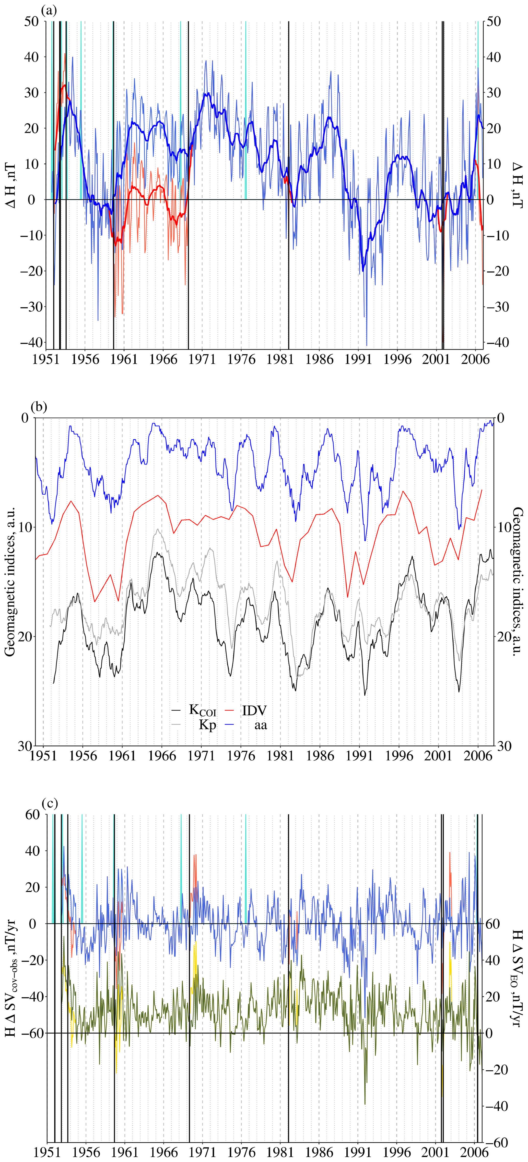
Figure 3Same as Fig. 2 but for the AdB period of measurements: 1951–2006. On (b) the monthly sums of the local KCOI (grey) and the global Kp (black) indices are also shown.

Differences between measurements and simulations arise not only from artificial inhomogeneities in the measured series but also from natural sources, e.g., solar and geomagnetic activity and crustal and induced fields that are not accounted for by the COV-OBS model. The H, I and Z series were found to be more strongly influenced by the solar activity than the D series analyzed in Morozova et al. (2014). In order to take this natural variability into account we used, as a third type of reference series, the following indices to describe the geomagnetic activity level (see Figs. 2b–5b): the index of inter-diurnal variability (IDV) from 1872 onward (Svalgaard et al., 2004; Svalgaard and Cliver, 2005); the aa index from 1868 onward; the global Kp index from 1951 onward (Menvielle et al., 2011); and the local KCOI index from 1951 onward, already homogenized in Morozova et al. (2014). The IDV and aa indices are global geomagnetic indices with the longest available series. They were used to estimate geomagnetic activity variation for the epoch before 1951 when the K index was introduced. The IDV, aa and K indices are calculated using different methodology, and, consequently, their variations may represent different features of geomagnetic activity; moreover, the difference between the Kp and KCOI indices reflect differences in the geomagnetic activity on the global and regional scales. Thus all these indices can be useful in the detection of homogeneity breaks in the series of geomagnetic field components related to the natural sources. The geomagnetic indices were used only for visualization of the geomagnetic cycles of external origin and for estimations of the approximate dates of the geomagnetic activity's minima and maxima.
The corrections for the artificial HBs (δ values) were calculated using the information from the Coimbra Magnetic Observatory's yearbooks and logbooks as well as by comparing the values of the measured components during some time intervals before and after a break in question (see details in Sect. 3).
Although the COV-OBS simulations cannot give the base level for COI, a more or less constant difference is expected between data series and COV-OBS simulations due to (1) uncertainty of the simulation, although the uncertainty of COV-OBS model changes a lot in time, being larger for ancient epochs, and (2) the crustal field. Assuming that the difference between the observations and COV-OBS is constant in time (slightly varying due to the geomagnetic activity cycles, see Sect. 3) and for a lack of better choice of the baselines, we choose to use the COV-OBS model level as an approximation for the actual base level of COI geomagnetic field components. We also paid attention to the cycles of the solar and geomagnetic activity so as to not overcorrect the observational data. Thus, in some cases, when COI data vary smoothly around the COV-OBS level and when these variations were in agreement with variations of geomagnetic indices, no corrections were applied. Please see detailed descriptions of specific cases in Sect. 3.
The HB corrections were applied backward in time, starting from the most recent break resulting in a corrected series in line with the most recent measurements. This is a procedure usually applied for homogenization of the meteorological data (Morozova and Valente, 2012a); however it may not always work for the COI series due to the long data gap between the 1940s and 1951. Nevertheless, all HBs are described here in direct chronological order in order to keep the usual narrative timeline.
The quality of the applied correction was estimated by calculation of (1) the homogeneity test statistics for the homogenized series and (2) the centered root mean square error parameter (CRMSE, see, e.g., Taylor, 2001; Venema et al., 2012). The CRMSE was calculated using Eq. (1):
where σD and σR are the standard deviations of the analyzed and reference series, respectively, and r is the Pearson correlation coefficient between the analyzed and reference series. In case the corrected series is more homogeneous than the original one, the CRMSE values for the corrected series will be lower than for the original (Venema et al., 2012). To compare the CRMSE obtained for different geomagnetic elements and their derivatives, the CRMSE values shown here are normalized: they are divided by the standard deviations of corresponding original series.
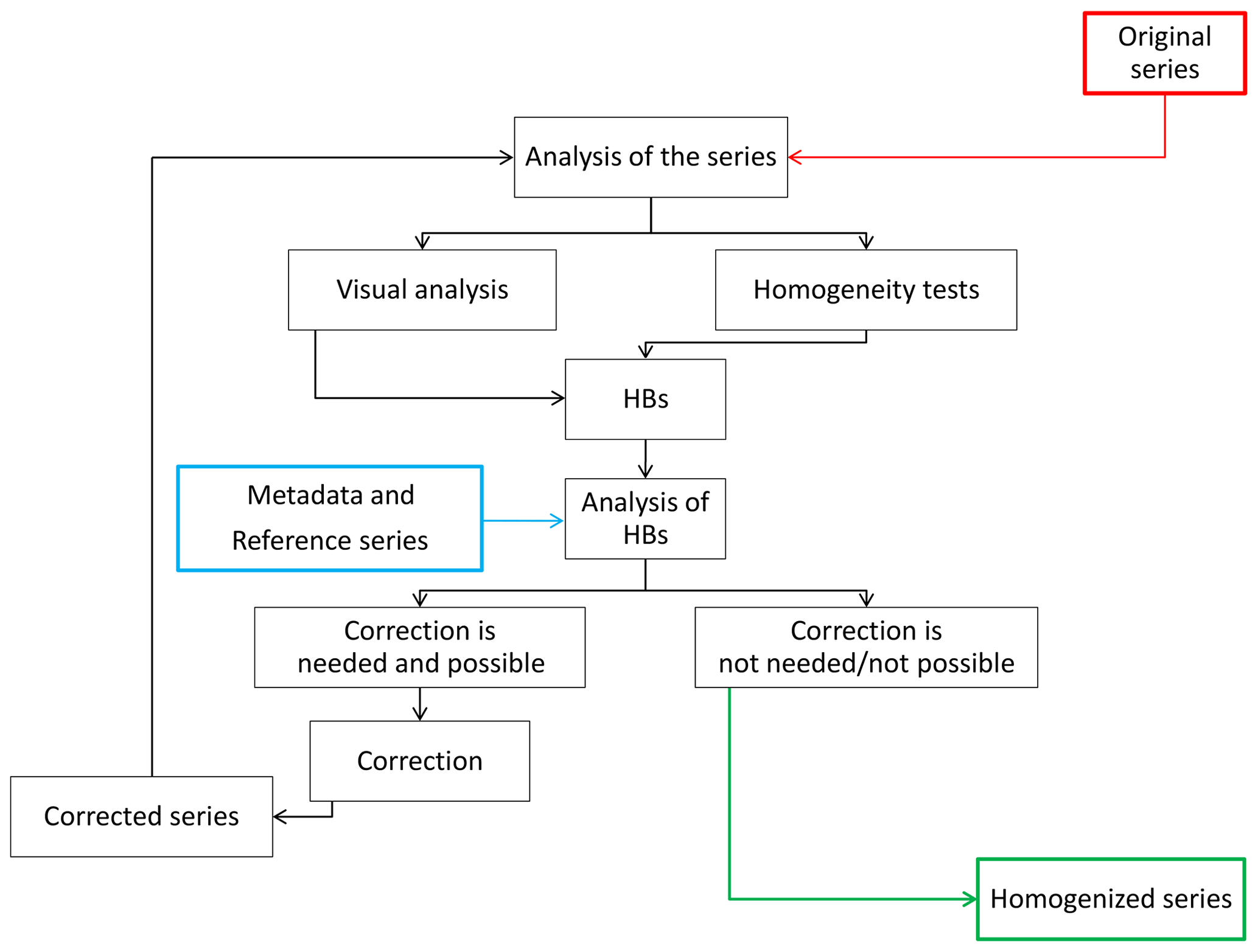
To summarize, the homogenization procedure consists of the following steps (see also Fig. 6).
-
The first step is the preliminary analysis of the series by correcting typos and OCR (optical character recognition) errors; detecting outliers; and calculating the Δ, SV and ΔSV series.
-
The second step is the visual analysis of the data and performing of statistical homogeneity tests.
-
The third step is the detection and analysis of HBs as follows:
- 1.
HBs with a statistical significance of at least 95 % are selected.
- 2.
Available metadata and logbooks are checked.
- 3.
If the homogeneity test detects an HB with a significance <95 % and a change is registered in the yearbooks, this break can also be accepted for correction.
- 4.
In the case of HBs with a statistical significance of at least 95 % not coinciding with changes registered in the yearbooks but coinciding with HBs in the series of geomagnetic indices, these HBs are excluded from the correction, as they were caused by solar and geomagnetic activity variations.
- 1.
-
The fourth step is the correction of the selected breaks using the most appropriate method discussed in Sect. 3.1–3.3.
-
The fifth step is the examination of the corrected series through the visual analysis, statistical homogeneity tests and CRMSE analysis.
The original and corrected series of the H, I and Z components and corresponding Δ, ΔSV and SV series are shown in Figs. 2–9 and S1. The results of homogeneity tests for the original and corrected series are shown in Figs. S3–S9.
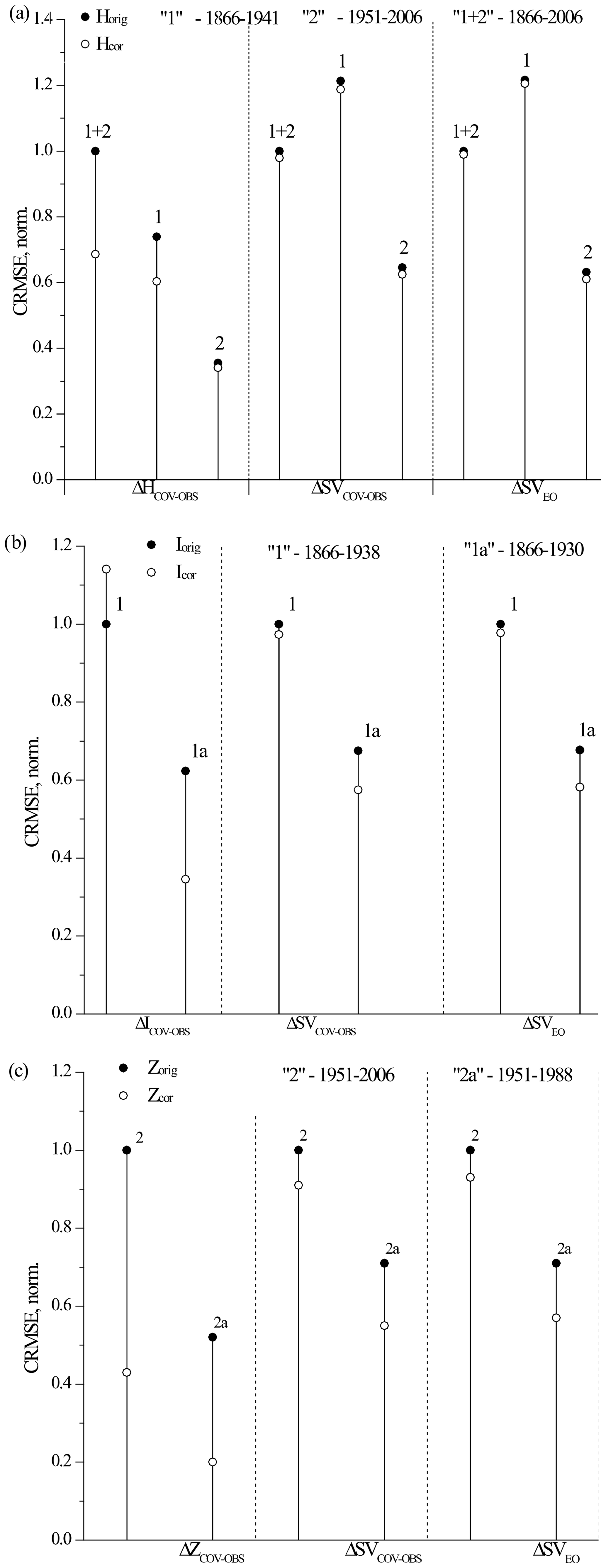
Figure 7CRMSE of the original (black dots; orig) and corrected (white filled circles; cor) COI series estimated for different time intervals: (a) COI H, (b) COI I and (c) COI Z. CRMSE values are normalized by the standard deviations of the original series.
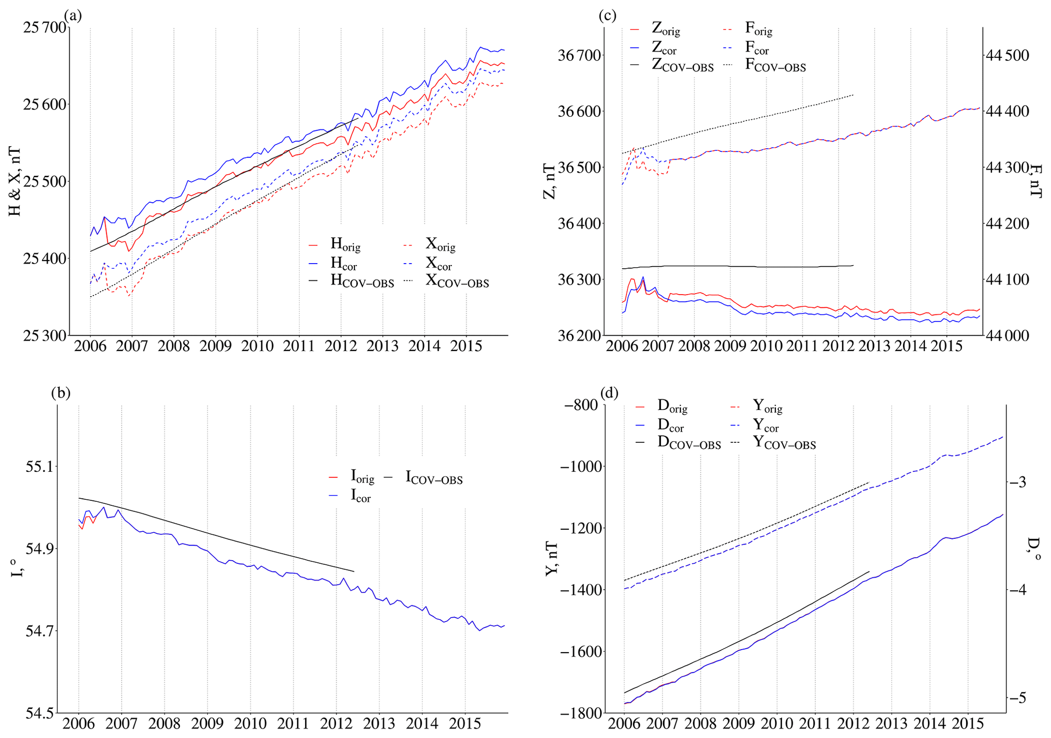
Figure 8For the 2006–2015 time period, measured (red; orig) and corrected (blue; cor) series of the COI geomagnetic field elements (a) H and X, (b) I, (c) F and Z, and (d) D and Y. The COV-OBS model predictions are in black.
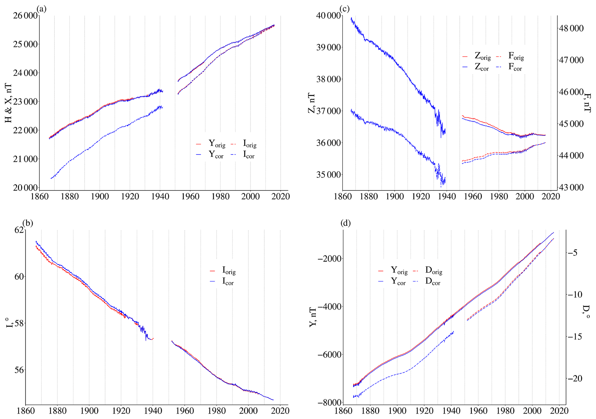
Figure 9For the 1866–2015 time period, measured (red; orig) and corrected (blue; cor) series of the COI geomagnetic field elements (a) H and X, (b) I, (c) F and Z, and (d) D and Y.
3.1 H component
The measured COI H monthly means series (H) can be split into two parts separated by a gap of about 10 years. The first time interval, from June 1866 to December 1941, contains measurements at the Cumeada and Alto da Baleia sites (C–AdB period); the second time interval, from October 1951 to May 2006, is related solely to the Alto da Baleia site (AdB period) (see Figs. 1a, 2–3, S1a–b and S3–S5 and Tables 1 and S3). The series were checked with yearbooks and logbooks for typos and OCR errors. Only absolute measurements are taken into account. Unfortunately, logbooks and yearbooks do not provide enough information about all changes to the measurement procedures and instrument repairs. Some records are too laconic; e.g., “some problems” are mentioned in logbooks without any description of their nature. Also, the analysis of the logbooks showed that from time to time observers (for different reasons) did not follow the recommended routine (e.g., monthly means can be calculated using only 1 or 2 weeks of measurements). As a result, there are inhomogeneities that cannot be confirmed by metadata. On the other hand, some events that could in principle generate inhomogeneities (e.g., installation of a new instrument) did not produce a visible and statistically significant HB. This is the case of the installation of a new instrument in January 1878 (Elliott unifilar) for measuring H and D components. It is possible that during the installation process the new instrument was calibrated in line with the old one without the corresponding note added to the logbook. The aging of the instruments, an increase of the urban electromagnetic noise (the beginning of the electrical-tram services in the nearby area) and other technical problems started to significantly affect the quality of the H data after 1929 (seen in the pink area of Fig. S10a as increased month-to-month variations). This situation did not improve during the first years after the relocation in January 1932. This is clearly seen in the dispersion of the monthly H data (see Figs. 2a and c and S10a). Only after the installation of the new instruments in 1951–1952 did the data quality improve (see Figs. 3a and c and S10a). This irregular behavior is also detected by the homogeneity test statistics (Fig. S3). To reduce the influence of this odd time period, homogeneity tests were calculated for two time intervals: from 1866 to 1941 (whole C–AdB period) and from 1866 to 1933 (a period excluding the epoch of major irregularities) (see Fig. S4).
The analysis of the first part of the H series showed that there were two statistically significant HBs (see Table 1): around March–April 1922 and from July to October 1931. In our opinion, the main reason for the break in March–April 1922 is the construction of a building within about 50 m from the house with absolute instruments. Despite the fact that there is no clear confirmation of this date in the observatory logbooks and yearbooks, it was chosen for the corrections both because it is clearly seen in the visual analysis and due to its high statistical significance (>99 %, Figs. S3–S4). The latter HB, or, more precisely, a 4-month-long jump of the mean level in July–October 1931 (Fig. 2), was likely caused by a lack of regular measurements during this time interval, which resulted in an artificially high level of the average monthly values. This conclusion is based on the analysis of the records and notes in the observatory's logbooks. Also, this break nearly corresponds to the relocation period, and it is likely that the routines had changed with consequences in the data quality. Therefore, this HB was also chosen for correction.
These two HBs are not the only features that can be detected in the analysis of the H series during the C–AdB period. First of all, we have to mention a long-term wave-like variation with minima around 1892 and 1932 and maxima around 1873–1878 and 1912 clearly seen in ΔH and SV (Figs. 2a and S1a, red lines). This variation is detected by the homogeneity tests applied to ΔH with a maximum of the SNHT statistics in 1880s (Figs. S3–S4). This variation is not seen in the ΔSV series (see Fig. 2c and corresponding homogeneity test results in Figs. S3b–S4b). We compared ΔH COI series with similar Δ series (differences between the observations and the COV-OBS model predictions) from other observatories available for this time interval (see Table S5). For the period 1866–1940 there are data from eight observatories: Parc Saint-Maur (PSM), Perpignan (PER), San Fernando (SFS), Oslo (OSL), Prague (PRA), Greenwich (GRW), Munich (MNH) and Lisbon (LIS); however the data sets of the MNH and LIS observatories have many gaps and contain clear shifts of the baseline (probably caused by changes to the observatory location, instruments or measurement procedure). The Δ series for the H component measured at the remaining six stations are shown in Fig. S11. The data observed at the observatories closest to COI observatories, SFS and PER, also show similar wave-like variations; similar variations are probably seen in the data of PRA, but since PRA data have a significant gap and were, probably, not homogenized, we cannot draw a final conclusion. On the other hand, the Δ series obtained from the PSM and OSL data show not a wave-like variation but rather a steady increase. Finally, the trend of the Δ series obtained from the GRW data is ambiguous.
Therefore, taking into account the absence of the recorded changes to the station environment and the similarity between the time variations of the series measured by COI and the closest observatories, we conclude that the observed long-term variations are due to the natural evolution of the geomagnetic field unaccounted for by the COV-OBS model.
The ΔH series also shows quasi-periodic decadal variations. These variations can also be found in the SV series, but there they are blurred by the high variability of the data. The origin of these quasi-decadal variations is clearly in the changes of the solar (and, consequently, geomagnetic) activity level. Figure 2 shows variations of the ΔH and ΔSVCOV−OBS series (panels a and c, respectively, red lines) alongside the variations of the aa and IDV indices (panel b). As one can see, the highest geomagnetic activity corresponds to lower values of ΔH. On the contrary, the periods of low geomagnetic activity correlate with epochs of higher ΔH values. Although this variability has a natural origin, from the statistical point of view it results in inhomogeneities detected by homogeneity tests (see Figs. S3–S4). Nevertheless, the variations of geomagnetic indices confirm the natural origin of these quasi-decadal variations of H and that they must be kept in the data.
Thus, only two HBs found during the C–AdB period were selected for correction (in 1922 and 1931, see Table 1). The correction values (δH, Table 1) were calculated as the difference between the means of the original ΔH series calculated for a certain time interval before and after the date of the HB. For the first HB this time interval was chosen to be 12 months. For the second HB the length of this time interval was only 4 months – the time between the break (July 1931) and the end of the series (October 1931). The corrections were rounded to the nearest whole number (since the precision of the 19th-century instruments was not higher than 1 nT). The corrected H, ΔH, SV and ΔSVCOV−OBS series are shown in Figs. 2a and S1a as blue lines, and the homogeneity test results for the corrected series are also shown in Figs. S3–S4.
According to the COI annual books and logbooks (Tables 1 and S3), the old instrument was kept in use for the first 3 months of the AdB period. Then, in January 1952, a set of new instruments was installed. The difference between the old and new instruments was considered “insignificant”. Later, in November 1952, the old magnetometers were compared to the newly purchased ones. According to the logbooks, the difference between the new and old instruments was about 20 nT. This information is supported by the visual analysis of the ΔH series (Fig. 3a): there is a visible shift of the main level of the ΔH series not related to the geomagnetic activity variations (represented by the geomagnetic aa, IDV, Kp and KCOI indices in Fig. 3b).
Later, in September 1953, the comparison between the measurements by the new and old instruments showed that the new H values were higher by about 5.4 nT. This change of the mean level is also seen in the visual analysis. The other comparison of the COI and reference instruments took place in August 1959. Both the visual analysis and homogeneity tests show no significant changes in the main level of the data at this date. We assume that for this time period the difference was too low to be seen comparing to the level of the monthly data variability.
One more comparison between the COI and reference instruments took place in April 1968. The differences were found to be about 18 nT. However, the analysis of the ΔH series shows that this correction has been applied up to April 1969. The last recorded comparison of the COI and reference instruments in August 1976 seems to cause no shifts of the H series that can be detected by the visual analysis or homogeneity tests.
There are also two outliers, February 1982 and October–December 2001, respectively, that have no direct documental support; however, as mentioned in the logbooks, in October 2001 the absolute measurements were taken only during the third week of the month, and we consider this as a possible source for the latter outlier.
The analysis of the homogeneity test statistics (see Fig. S5) shows that the ΔH and ΔSVCOV−OBS series contain both the artificial inhomogeneities (abovementioned shifts and outliers) and the natural periodicities related (mostly) to the solar and geomagnetic cycles. Taking into account the results of the visual analysis, homogeneity tests and logbook records, we selected only five HBs for the corrections, listed in Table 1. The corrections for HBs associated with comparison to the reference instruments mentioned above were taken from the logbooks, and the corrections for the outliers were calculated as differences between the means of the original ΔH series 4 months before and after each of the outliers in 1982 and before the beginning and after the end of the outlier interval in 2001 (see values in Table 1). Such a short time interval was chosen to avoid contamination from the cyclic variations of the geomagnetic activity (compare Fig. 2a and 2b). The corrections were rounded to the nearest whole number (the precision of the instruments was 1 nT). The corrected series are shown in Figs. 3 and S1a as blue lines, and the homogeneity test results for the corrected series are also shown in Fig. S5 in the Supplement.
In some cases the corrections of the artificial HBs resulted in an increase of the statistical significance of the “natural HB” related to the geomagnetic cycles (Fig. S5a). The fact that this behavior is seen mostly during the AdB period can be due to the higher precision of the new instruments; another possible reason is the increase of the geomagnetic activity in the second half of the 20th century reported by, e.g., Love (2011). Based on the variations of the geomagnetic indices, we conclude that the maxima observed on the SNHT statistics around the 1980s, 1990s and 2000s (seen in Fig. S5a) are due to the natural variability of the data and do not need correction.
The CRMSE values for the original and corrected H and SV series relative to the corresponding reference series are shown in Fig. 7a. The results of this analysis support the conclusion that the corrected series are more homogeneous than the original ones; however, they contain “natural” inhomogeneities related, in particular, to the variations of the solar and geomagnetic activity.
3.2 I component
The digital series of the I monthly absolute measurements available from different sources (including the website of the World Data Centre for Geomagnetism, Edinburgh, UK) starts in June 1866 and ends in May 1940. The series contains a number of gaps (from 1 to 6 months long, with longer gaps clustered between 1936 and 1940). This series was checked for OCR errors, typos and calculation errors. The homogeneity of the series was affected by the relocation of the observatory (in 1932), repair and replacement of instruments or their parts, and environmental changes (urban electromagnetic noise level). The I series and its derivatives are shown in Figs. 1b, 4 and S1b. As one can see, between 1866 and 1932 the Δ and ΔSV series (Fig. 4a and c) show fluctuations related both to the already known changes to the instruments and procedures and to the variations of the solar activity (as is clearly seen in Fig. 4b, where the IDV and aa geomagnetic indices are plotted): the Δ series varies in phase with IDV and aa. However, starting from about 1931 the I series shows a strong and unexpected decrease that can be explained neither by natural variations of the field nor by events mentioned in the metadata. The most likely explanation is the degradation or incorrect installation of the instruments and needles or other (human) factors (e.g., disregard of the measurement procedures). Besides, the records in the logbooks clearly state that the I component was measured at COI only until the end of 1938. The origin of the (highly fragmented) monthly values of I between January 1939 and May 1940 is unknown. Therefore, we strongly recommend not to use the COI I series for this period, and, accordingly, the I values for this time interval are removed from the final homogenized version described in this work.
The COI I series containing the measurements between 1866 and 1938 was submitted to the homogenization procedure. The homogeneity test statistics were calculated both for the whole interval (1866–1938) and for a shorter time interval (1866–1930), shown in Figs. S6–S7, respectively, to exclude the period of the fast decrease. Both the visual analysis (Fig. 4) and the statistical homogeneity tests (Figs. S6–S7) show a number of HBs that are related to the known changes to the instruments or station location (see Tables 2 and S3). These dates are September 1876, November 1922, September 1928, January 1931, January 1932 and January 1939. There is also an HB in May 1883 that is seen in the homogeneity tests of the ΔSVCOV−OBS series (Fig. S7b); however the yearbooks and logbooks of the observatory contain no information that can be related to this HB. The comparison of the Δ and the geomagnetic indices series (Fig. 4) shows that this HB is of natural origin and is related to a sharp decrease in the geomagnetic activity. Thus, this HB was not corrected. It has to be mentioned that the analysis of the data for the time interval of 1931–1932 led us to assume that although the logbook records mention that during 1931 the measurements were taken at the Cumeada and the Alto da Baleia sites simultaneously, the published measurements, most likely, were obtained at the new site. Furthermore, the change of the instrument in October 1935 (the old inclinometer was replaced by an earth inductor), during the period of the fast decrease of I seen both in the visual analysis and homogeneity tests, cannot be corrected due to the overall bad quality of the data.
As shown in Fig. 4a, during the time interval from November 1922 to August 1928 the Δ series slowly fluctuates (due to geomagnetic activity cycles) around zero, meaning that the differences between the measured and simulated I values do not have any systematic shift or trend. Assuming that there is no reason for a sudden (on the timescale of 1 month) change of the base level of the order of 5–10′, we decided to use the COV-OBS model as an approximation for the actual COI I base level. Therefore, the time interval from November 1922 to August 1928 was chosen as a reference interval: the corrections for the I series were calculated in a way that the mean values of Δ for any interval between HBs were equal to zero (the average value of Δ for the homogeneous interval from November 1922 to August 1928). Three time intervals between HBs were corrected (Table 2): June 1866–August 1876, September 1876–October 1922 and September 1928–December 1930. The corrections were rounded to 1′ (according to the precision of the instrument). The time interval between January 1931 and December 1938 was not corrected due to the bad data quality and strong decreasing trend. The corrected I series and its derivatives are shown in Figs. 4 and S1b (blue lines), and corresponding homogeneity test statistics are in Figs. S6–S7. The homogeneity test statistics for the corrected I series still show statistically significant HBs related to geomagnetic activity cycles. The CRMSEs calculated for the original and the corrected series are shown in Fig. 7b. The CRMSEs for the corrected series are lower than for the original. Thus, the corrected I series is more homogeneous than the original one and contains, mostly, variations related to the natural sources, except the period from 1931 to 1938 which we do not recommend to use for any scientific analysis or simulation.
3.3 Z component
The installation of a new BMZ instrument in January 1953 is seen in the Z records (Figs. 1c, 5 and S1c) as a sudden step-like change of the baseline by about 30 nT. The visual analysis of the Z and ΔZ series (Figs. 1c and 5) show that after about 1.5 years from that date some problems with the instrument or measurement procedures started to appear: the level of the Z series jumped up by about 20 nT in the middle of 1954 and again by about 10 nT at the end of 1955. Yet another increase of the base level for Z series took place at the end of 1960. The reasons for these changes are unknown, since the currently available logbooks do not contain any notes on the Z measurements until 1963. However, these jumps cannot be neglected, since they are seen not only in the visual analysis but also in the relative homogeneity tests of both the Δ and ΔSVCOV−OBS series (see Figs. S8–S9). These HBs do not coincide with the cycles of the geomagnetic activity (see geomagnetic indices aa, IDV, Kp and KCOI in Fig. 5b), and they are too sharp for the monthly mean data (see also Fig. S10c) to be attributed to the solar activity effect. They are also not seen in the variations of the SVEO series (Fig. S1d). A replacement of the instrument took place in January 1977, but no HBs were found near this date. Two HBs were detected around September 1971 and December 1973. It seems that some measures were taken to improve the quality of the Z measurements at COI: from December 1973 the base line of the recorded measurements is in a good agreement with simulation done by the COV-OBS models. This homogeneous period started to deteriorate around 1982 when an annual cycle appeared in the data. This cycle became more prominent around 1989. Besides, the decrease of the mean Δ in 1990–1991 was too steep compared to the variations of the geomagnetic indices (Fig. 5b). Similarly to the I component, we decided to use COV-OBS model as an approximation for the actual COI Z base level assuming that there are no natural sources for sudden (on the timescale of 1 month) changes of the base level of the order of 5–20 nT.
The origin of the annual cycle (and, probably, a part of the overall decrease of the Z base level between 1990 and 2006) seems to be related to the degradation of the instruments (the precision of the instruments to the temperature variations strongly increased) or, perhaps, errors in the calculation due to non-application of the temperature correction factor (or application of a wrong factor). This assumption is supported by the comparison of the monthly mean ΔZ values with the monthly mean temperature parameters measured by the Coimbra Meteorological Observatory (see Morozova and Valente, 2012a) – daily minimum (Tmin) and maximum (Tmax) temperatures (see Fig. S12). For the time interval of 1990–2006 the correlation coefficients between the ΔZ and meteorological series are about 0.7 (p≤0.01, calculated using a Monte Carlo approach with artificial series constructed using a procedure of bootstrapping with moving blocks, with a block length equal to 12 months).
After the visual and statistical analysis of the Z, Δ and ΔSV series, several HBs classified as “artificial” were identified and selected for correction (please see also Figs. S8–S9). They are listed in Table 3 (see also Table S3).
The time interval of June 1954–October 1960 was divided into two: before and after October 1955. This additional HB, seen only in the visual analysis, was needed to avoid step-like variations in the corrected Z series. This HB seems to be too small to be seen in the homogeneity tests on the background of the signal from other breaks. However, it becomes visible and statistically significant if the corrections are applied to all other HBs. Similarly to the I component case, taking the value ΔZ=0 nT (the mean ΔZ value for the time period December 1973–October 1989) as the reference level, we calculated the correction value for this HB (see also Fig. 5).
The annual cycle (from 1990 to 2006) was not corrected because linear regression coefficients of the Z series on the temperature series change from year to year. It is possible that such corrections for the meteorological effect are nonlinear, should take the average humidity level into account and, also, depend on the mean annual level of the geomagnetic activity.
The corrected Z series and its derivatives are shown in Figs. 5 and S1c as blue lines. The homogeneity tests (Figs. S8–S9) show that the corrected series contain HBs coinciding with the geomagnetic activity cycles (e.g., the maximum in 1980s) and the annual temperature cycle in 1990–2006. The CRMSE values for the original and corrected Z and SV series relative to the corresponding reference series are shown in Fig. 7c. The CRMSE of the corrected Z series are lower than those of the original ones both when the whole series (1951–2006) and a shorter time interval (1951–1988) are considered. The results of this analysis show that the corrected series are more homogeneous than the original ones; however, they still contain natural inhomogeneities related to the variations of the solar and geomagnetic activity and the meteorological effect for the 1990–2006 time interval.
To complete the procedure of the homogenization of the historical COI geomagnetic series, the series for all geomagnetic elements (X, Y, Z, H, D, I and F) were obtained for the period 1866–2006 using the direct measurements for some elements and calculating the other elements from the measurements as described below. The series of the geomagnetic elements were homogenized in line with most recent values in the series used for this study, i.e., December 2015. The uncorrected and corrected series for the time interval of 2006–2015 are shown in Fig. 8 together with the COV-OBS predictions.
First of all, we compared measured series before and after 2006 to make necessary corrections. To keep the D series in line with current measurements, we introduced additional correction to the series previously homogenized in Morozova et al. (2014). The correction for the D series of (considering the difference between the monthly values of December 2005 and January 2006) was applied to the series between June 1866 and December 2005. The correction for the I component before June 2006 is not necessary, since there is no visible jump. The corrections for the F series were calculated backward in time, first for the data before May 2007 (the change of the instrument implied a jump in the baseline between the months of April and May 2007) and later for the data before June 2006. The corrections were calculated assuming that the average change of the F values on the monthly scale is about +10 nT yr−1 or +0.83 nT per month, which is the average rate of change of F between June 2007 and December 2015. The correction of 22 nT for F was applied only for the June 2006–May 2007 time period. From the corrected D and F and the uncorrected I series the new series of H and Z for the 2006–2015 time interval were recalculated. As a result, no visible breaks were seen in the H series, whereas there seems to be a significant jump (about 59 nT) in the Z series. This correction was applied to the whole period from October 1951 to December 2005. Please note that this correction also solved the problem of the voluntarily chosen baseline level when the Z series for the 1951–2006 time interval was corrected (see Sect. 3.3).
Afterwards, all the elements (except D) were calculated for those periods where they were not measured:
-
Z for May 1864–December 1938 (from the H and I data),
-
F for May 1864–December 1938 (from H and I) and October 1951–May 2006 (from H and Z), and
-
I for October 1951–May 2006 (from H and Z).
Also, the X and Y components were calculated from July 1867 (beginning of the D observations) to December 2015. All the series except the D series have a gap in the data (from 1938–1941 to 1951). The series before the gap were not homogenized in line with the current observations both because of the gap and due to the bad quality of the data at the end of the C–AdB period. As was mentioned above, in most cases, the COV-OBS predictions were used as a reference level for the 1866–1951 time interval. All the series of the COI geomagnetic field elements (original and corrected) are shown in Fig. 9 (red and blue lines, respectively).
The COI geomagnetic field elements are available via the following addresses: https://doi.org/10.5281/zenodo.4308022 (Ribeiro et al., 2020) for the original COI data (ASCII and XLSX formats) and https://doi.org/10.5281/zenodo.4308036 (Morozova et al., 2020) for the homogenized COI data (ASCII and XLSX formats).
The historical temperature series of the Coimbra Magnetic Observatory are available at https://doi.org/10.1594/PANGAEA.785377 (Morozova and Valente, 2012b).
The COI data series for 2016–2017 can be downloaded from the database of the World Data Centre for Geomagnetism, Edinburgh (http://www.wdc.bgs.ac.uk/dataportal/, last access: 1 March 2021).
The IDV index can be downloaded from the website of Leif Svalgaard, http://www.leif.org/research/ (last access: 1 March 2021).
The aa index is available from the NGDC (National Centers for Environmental Information, formerly National Geophysical Data Center) website at http://www.ngdc.noaa.gov/stp/spaceweather.html (last access: 1 March 2021).
The global Kp index can be downloaded from https://doi.org/10.5880/Kp.0001 (Matzka et al., 2021, see https://www.gfz-potsdam.de/kp-index/, last access: 1 March 2021, for a general overview) or http://isgi.cetp.ipsl.fr/des_kp_ind.html (last access: 1 March 2021).
As a continuation of the previous work (Morozova et al., 2014) on the homogenization of the historical series of the Coimbra Magnetic Observatory (COI), Portugal, we applied here a similar type of analysis to the long time series of H (horizontal component), Z (vertical component) and I (inclination) absolute monthly means. The H component was measured from 1866 to 2006 with a break of about 10 years in the middle of 20th century; the I component was measured from 1866 to 1938; and the Z records are from 1951 to 2006. Monthly mean values of the analyzed parameters and their time derivatives were studied relative to the data series from both other European observatories, and predictions were made for the Coimbra location by the COV-OBS model of the geomagnetic field. The analysis was done using available metadata (logbooks and annual books of the observatory), the visual analysis of the series and the SNHT statistical homogeneity test. Changes of the geomagnetic activity were accounted for by the comparison to the geomagnetic activity indices (aa, IDV, Kp and local KCOI index). Statistically significant homogeneity breaks of artificial (non-natural) origin were detected and whenever possible corrected. The corrected series were tested for homogeneity.
Overall, the corrected series show more consistency with the data from other geomagnetic observatories. The series recorded after 1951 (the Z and the second part of the H series) have better data quality compared to the series recorded during the 19th and the first half of the 20th centuries, allowing for a much easier detection and correction of the homogeneity breaks. This, mostly, results from a better quality of the instruments (higher precision) and improved observation procedures. Unfortunately, the corrected series still contain artificial inhomogeneities related, in particular, to the degradation of the instruments and an increase of the urban electromagnetic noise.
No treatment to remove the urban noise was applied in this work. The level of the urban electromagnetic noise could be devised, for example, from the variability of the data, e.g., using the month-to-month time derivative or the standard deviation by comparing a more perturbed period to a less perturbed period. Also, one must keep in mind that a larger part of hourly and daily noise is averaged out by the calculation of the monthly means. The final step of the homogenization of the COI series consisted in the homogenization of all the series to the level of the current measurements. The series of the F, D and I components available before 2006 were homogenized in line with the current observations. Then, the series of other elements were recalculated for the period 1866–2006 and, when needed, corrected for jumps. Please note that only the D series that is available for the entire COI lifetime duration (from 1866 to the present) is homogenized in line with the current COI measurements. For other elements, only those parts of the series that are available from 1951 are homogenized in line with the current COI measurements.
Currently, the original and homogenized series (ASCII and XLSX formats) are available at https://doi.org/10.5281/zenodo.4308022 and https://doi.org/10.5281/zenodo.4308036, respectively, and can be used in studies of secular variation. The COI data series for 2016–2017 can be downloaded from the database of the World Data Centre for Geomagnetism, Edinburgh (http://www.wdc.bgs.ac.uk/dataportal/, last access: 1 March 2021), and added to the homogenized series without any further correction. The data for 2018 and 2019 will be uploaded to the World Data Centre for Geomagnetism (WDC) database soon. Besides, the metadata for the COI historical geomagnetic series are also summarized in Tables S1–S4. During the second half of the 19th and first half of the 20th centuries, historical observatories represent the main source of highly dynamic and relatively precise geomagnetic data. We believe that applying this kind of study to other historical series can contribute to better constrain geomagnetic field models such as COV-OBS and also better characterize cycles of external geomagnetic activity during the pre-satellite era.
The supplement related to this article is available online at: https://doi.org/10.5194/essd-13-809-2021-supplement.
PR provided digital series of the COI geomagnetic field elements and worked with the logbooks and annual books. MAP provided COV-OBS simulations. ALM performed visual and statistical analyses of the series and estimated corrections. ALM prepared the paper; PR and MAP revised the paper.
The authors declare that they have no conflict of interest.
Authors are grateful to Mioara Mandea and Vadim Soldatov for useful comments which resulted in the improvement of the paper.
CITEUC is funded by national funds through the FCT (Fundação para a Ciência e a Tecnologia) projects UID/00611/2020 and UIDP/00611/2020.
Anna L. Morozova thanks the Geophysical and Astronomical Observatory of the University of Coimbra and João Fernandes for financial support of this work.
M. Alexandra Pais wishes to thank Nicolas Gillet for kindly computing the COV-OBS w/o COI model that was used in this study.
This research has been supported by the Fundação para a Ciência e a Tecnologia (grant nos. PTDC/CTA-GEO/31744/2017 and PTDC.FER-HFC.30666).
This paper was edited by Kirsten Elger and reviewed by Mioara Mandea and Vadim Soldatov.
Alexandersson, H. and Moberg, A.: Homogenization of Swedish temperature data. Part I: Homogeneity test for linear trends, Int. J. Climatol., 17, 25–34, 1997.
Costa, A. C. and Soares, A.: Homogenization of climate data: review and new perspectives using geostatistics, Math. Geosci., 41, 291–305, 2009.
Gillet, N., Jault, D., Finlay, C. C., and Olsen, N.: Stochastic modeling of the Earth's magnetic field: Inversion for covariances over the observatory era, Geochem. Geophys. Geosys., 14, 766–786, 2013.
Love, J. J.: Secular trends in storm-level geomagnetic activity, Ann. Geophys., 29, 251–262, https://doi.org/10.5194/angeo-29-251-2011, 2011.
Matzka, J., Bronkalla, O., Tornow, K., Elger, K., and Stolle, C.: Geomagnetic Kp index. V. 1.0, GFZ Data Services, https://doi.org/10.5880/Kp.0001, 2021.
Menvielle, M., Iyemori, T., Marchaudon, A., and Nosé, M.: Geomagnetic Indices, in: Geomagnetic Observations and Models (Vol. 5), edited by: Mandea, M. and Korte, M., Springer, Dordrecht Heidelberg London New York, 183–228, https://doi.org/10.1007/978-481-9858-0, 2011.
Morozova, A. L. and Valente, M. A.: Homogenization of Portuguese long-term temperature data series: Lisbon, Coimbra and Porto, Earth Syst. Sci. Data, 4, 187–213, https://doi.org/10.5194/essd-4-187-2012, 2012a.
Morozova, A. L. and Valente, M. A.: Homogenization of Portuguese long-term temperature data series: Lisbon, Coimbra and Porto, PANGAEA, https://doi.org/10.1594/PANGAEA.785377, 2012b.
Morozova, A. L., Ribeiro, P., and Pais, M. A.: Correction of artificial jumps in the historical geomagnetic measurements of Coimbra Observatory, Portugal, Ann. Geophys., 32, 19–40, https://doi.org/10.5194/angeo-32-19-2014, 2014.
Morozova, A., Ribeiro, P., and Pais, M. A.: Homogenized monthly datasets of all geomagnetic components of Coimbra observatory for the time period 1866–2015, Zenodo, https://doi.org/10.5281/zenodo.4308036, 2020.
Pais, M. A. and Miranda, J. M. A.: Secular variation in Coimbra (Portugal) since 1866, J. Geomagn. Geoelectr., 47, 267–282, 1995.
Parkinson, W. D.: Introduction to geomagnetism, Scottish Academic Press, United States, 433 p., 1983.
Ribeiro, P., Pais, M. A., and Morozova, A. L.: Monthly values of absolutely measured geomagnetic components (D, I, H, Z, F) of Coimbra observatory in the period 1866–2015, Zenodo, https://doi.org/10.5281/zenodo.4308022, 2020.
Svalgaard, L. and Cliver, E. W.: The IDV index: Its derivation and use in inferring long-term variations of the interplanetary magnetic field strength, J. Geophys. Res., 110, 1–9, 2005.
Svalgaard, L., Cliver, E. W., and Le Sager, P.: IHV: A new long-term geomagnetic index, Adv. Space Res., 34, 436–439, 2004.
Taylor, K. E.: Summarizing multiple aspects of model performance in a single diagram, J. Geophys. Res., 106, 7183–7192, 2001.
Venema, V. K. C., Mestre, O., Aguilar, E., Auer, I., Guijarro, J. A., Domonkos, P., Vertacnik, G., Szentimrey, T., Stepanek, P., Zahradnicek, P., Viarre, J., Müller-Westermeier, G., Lakatos, M., Williams, C. N., Menne, M. J., Lindau, R., Rasol, D., Rustemeier, E., Kolokythas, K., Marinova, T., Andresen, L., Acquaotta, F., Fratianni, S., Cheval, S., Klancar, M., Brunetti, M., Gruber, C., Prohom Duran, M., Likso, T., Esteban, P., and Brandsma, T.: Benchmarking homogenization algorithms for monthly data, Clim. Past, 8, 89–115, https://doi.org/10.5194/cp-8-89-2012, 2012.
- Abstract
- COI metadata
- Homogenization procedure
- Homogenization of the COI series (1866–2006)
- Homogenization of the historical COI series in line with the current digital measurements (2006–2015)
- Data availability
- Conclusions
- Author contributions
- Competing interests
- Acknowledgements
- Financial support
- Review statement
- References
- Supplement