OceanSODA-ETHZ: a global gridded data set of the surface ocean carbonate system for seasonal to decadal studies of ocean acidification

Ocean acidification has profoundly altered the ocean's carbonate chemistry since preindustrial times, with potentially serious consequences for marine life. Yet, no long-term, global observation-based data set exists that allows us to study changes in ocean acidification for all carbonate system parameters over the last few decades. Here, we fill this gap and present a methodologically consistent global data set of all relevant surface ocean parameters, i.e., dissolved inorganic carbon (DIC), total alkalinity (TA), partial pressure of CO₂ (pCO₂), pH, and the saturation state with respect to mineral CaCO₃ (Ω) at a monthly resolution over the period 1985 through 2018 at a spatial resolution of $\mathrm{1}{}^{\circ }\times \mathrm{1}{}^{\circ }$. This data set, named OceanSODA-ETHZ, was created by extrapolating in time and space the surface ocean observations of pCO₂ (from the Surface Ocean CO₂ Atlas, SOCAT) and total alkalinity (TA; from the Global Ocean Data Analysis Project, GLODAP) using the newly developed Geospatial Random Cluster Ensemble Regression (GRaCER) method (code available at https://doi.org/10.5281/zenodo.4455354, Gregor, 2021). This method is based on a two-step (cluster-regression) approach but extends it by considering an ensemble of such cluster regressions, leading to improved robustness. Surface ocean DIC, pH, and Ω were then computed from the globally mapped pCO₂ and TA using the thermodynamic equations of the carbonate system. For the open ocean, the cluster-regression method estimates pCO₂ and TA with global near-zero biases and root mean squared errors of 12 µatm and 13 µmol kg⁻¹, respectively. Taking into account also the measurement and representation errors, the total uncertainty increases to 14 µatm and 21 µmol kg⁻¹, respectively. We assess the fidelity of the computed parameters by comparing them to direct observations from GLODAP, finding surface ocean pH and DIC global biases of near zero, as well as root mean squared errors of 0.023 and 16 µmol kg⁻¹, respectively. These uncertainties are very comparable to those expected by propagating the total uncertainty from pCO₂ and TA through the thermodynamic computations, indicating a robust and conservative assessment of the uncertainties. We illustrate the potential of this new data set by analyzing the climatological mean seasonal cycles of the different parameters of the surface ocean carbonate system, highlighting their commonalities and differences. Further, this data set provides a novel constraint on the global- and basin-scale trends in ocean acidification for all parameters. Concretely, we find for the period 1990 through 2018 global mean trends of 8.6 ± 0.1 µmol kg⁻¹ per decade for DIC, −0.016 ± 0.000 per decade for pH, 16.5 ± 0.1 µatm per decade for pCO₂, and −0.07 ± 0.00 per decade for Ω. The OceanSODA-ETHZ data can be downloaded from https://doi.org/10.25921/m5wx-ja34 (Gregor and Gruber, 2020).

1 Introduction

The oceans have taken up roughly one-quarter of the anthropogenic CO₂ that has been released into the atmosphere since the start of the industrial era (Sabine et al., 2004; Gruber et al., 2019), modulating the increase in atmospheric CO₂ substantially. However, this buffering of anthropogenic climate change by the ocean comes with a substantial cost, i.e., ocean acidification (Doney et al., 2009). The uptake of anthropogenic CO₂ over the last 150 years has made the surface ocean more acidic with a decrease in global mean pH from ∼ 8.2 around 1850 to ∼ 8.1 today (Feely et al., 2009; Jiang et al., 2019). This decrease in pH equates to a ∼ 30 % increase in the concentration of H⁺ ions. Some of the anthropogenic CO₂ taken up from the atmosphere remains in the seawater as dissolved CO₂, thus increasing its partial pressure (pCO₂). In fact, surface ocean pCO₂ tends to track the increase in atmospheric pCO₂ rather closely (e.g., Bates et al., 2014) owing to the ∼ 1-year timescale for the equilibration of CO₂ across the air–sea interface (Sarmiento and Gruber, 2006), which is smaller than the decadal timescale increase in atmospheric CO₂ (Friedlingstein et al., 2019). While some of the added CO₂ stays as CO₂, the majority of it is titrated away by the ocean's carbonate ion (Sarmiento and Gruber, 2006), leading to a substantial reduction in its concentration. This reduces the saturation state (Ω) with regard to the mineral calcium carbonate (CaCO₃), where an Ω of <1 leads to dissolution of CaCO₃.

These chemical changes, collectively described as ocean acidification, will have a profound impact on marine organisms, especially those that form shells made of CaCO₃ (Orr et al., 2005; Fabry et al., 2008; Doney et al., 2009; Bednaršek et al., 2019; Doney et al., 2020). Calcifying organisms living in high latitudes and subtropical and tropical upwelling regions, with their naturally low Ω and pH, may be particularly vulnerable, as these regions will be among the first to cross critical saturation thresholds (Orr et al., 2005; Steinacher et al., 2009; Gruber et al., 2012; Franco et al., 2018; Fabry et al., 2009; Hauri et al., 2016; Negrete-García et al., 2019). However, marine organisms may be susceptible to changes even where Ω >1 due to a shift in energetic requirements for shell formation (Orr et al., 2005; Pörtner and Farrell, 2008). For example, it is well known that corals start to decrease their calcification already at saturation states well above 3 (Gattuso et al., 1998). Ocean acidification will thus have a significant economic impact on fisheries and tourism through the impact on shellfish and corals, respectively (Cooley and Doney, 2009; Doney et al., 2020).

At the global scale, most of what we know about the progression of ocean acidification in the recent decades has come from either models (Bopp et al., 2013; Kwiatkowski et al., 2020) or from the combination of model-based trends with observation-based climatologies (Feely et al., 2009; Jiang et al., 2019). A notable exception is the large number of studies that have analyzed the trends and variability of surface ocean pCO₂ (e.g., Landschützer et al., 2013, 2016; Rödenbeck et al., 2014; Denvil-Sommer et al., 2019; Gregor et al., 2019) and the effort of Lauvset et al. (2015) and Turk et al. (2017) to analyze long-term trends in pH and Ω respectively. But these studies remained limited to one single parameter. At the local-to-regional scale, a number of long-term time series have provided excellent insights into the processes and trends of ocean acidification across all carbonate system parameters (e.g., Bates et al., 2014), but no global comprehensive view of the historical development of ocean acidification based on observations exists. This is largely a consequence of the limited observations, although observational efforts have increased substantially in the recent decades through efforts such as GOA-ON (Global Ocean Acidification Observing Network, Tilbrook et al., 2019). The OceanSODA (Satellite Oceanographic Datasets for Acidification) project (https://esa-oceansoda.org, last access: 12 September 2020), which this study forms part of, aims to close this gap by linking satellite observations with in situ observations of the marine carbonate system.

In line with the goal of the OceanSODA project, we aim to develop a global, observation-based data set documenting the progression of ocean acidification over the recent decades. Such a data set will be crucial to put the current trends of ocean acidification into the context of the changes over the last few decades. By also describing the level of variability in ocean acidification around the long-term trend, it will also help to better understand the challenges that marine organisms are facing. Additionally, it will permit us to explore in much more detail how ocean acidification has unfolded regionally and potentially deviated from the simple model of it being dependent on the rise in atmospheric CO₂.

The well-measurable parameters of the marine carbonate system are dissolved inorganic carbon (DIC), total alkalinity (TA), pH, and the partial pressure of carbon dioxide (pCO₂). Very few measurement programs measure all of these parameters concurrently. In fact, the vast majority of the observational programs measure only one parameter, with pCO₂ being the most often measured one, followed by DIC, TA, and pH (Bakker et al., 2016; Olsen et al., 2019). Since two parameters are sufficient to fully describe the marine carbonate system, any combination of two will permit us to fully reconstruct the entire carbonate system. But not all combination are equally suited, given the uncertainties in the measurements, the uncertainties in the coefficients of the carbonate chemistry, and the spatiotemporal coverage vis-à-vis the variability of these parameters.

We use here the pair pCO₂ and TA as the basis for our reconstruction for two reasons. First, these are the best observed parameters relative to their spatiotemporal variability, permitting us to develop better predictive models for the global surface ocean than possible for, e.g., DIC and pH. Second, detailed assessments of the internal consistency of the oceanic carbonate system have shown that pCO₂ and TA are a well-suited pair to estimate pH, owing to the reliability of the measurements and the predictive accuracy (Bockmon and Dickson, 2015; Bakker et al., 2016; Raimondi et al., 2019). This is not the case if DIC was used instead of TA. Our choice is supported by Takahashi et al. (2014), who developed the first seasonal climatology of all surface ocean carbonate system parameters using the same pair.

Measurements of pCO₂ are abundant compared to the other variables, due to a well-established and robust underway sampling protocol that allows instruments to also be installed on non-scientific vessels under the Voluntary Observing Ship (VOS) program (Bakker et al., 2016; Pierrot et al., 2009). High-quality pCO₂ data are also easily accessible thanks to the Surface Ocean CO₂ Atlas (SOCAT) that consolidates underway pCO₂ observations and ensures the quality of observations (Bakker et al., 2016). Total alkalinity is not as widely measured as pCO₂ due to the fact that measurements are made discretely with bottle samples (Dickson et al., 2007). But, fortunately, TA is highly correlated with salinity on a global scale (r=0.96), making it a suitable variable for prediction with a <10 % error of the observed range (Lee et al., 2006; Olsen et al., 2019; Broullón et al., 2018). Further, the accessibility of TA measurements is made possible through the continued efforts of the Global Ocean Data Analysis Project (GLODAP; Olsen et al., 2019). We discarded the option to use DIC instead of TA, even though DIC is slightly more often sampled than TA. This decision is based on the fact that DIC is more variable than TA, and also its correlation with salinity is much lower. As a result, it is difficult to develop predictive models for DIC that are as accurate and precise as those for TA. Oceanic pH is also not an option, since historically it has been measured far less often than the other parameters. This is changing, since progress with reference materials and new sensors have permitted a tremendous increase in the number of pH measurements in recent years, largely benefiting from deployments of biogeochemical Argo floats (Claustre et al., 2020).

The actual spatial and temporal coverage for any of these parameters is very low. Even for pCO₂, i.e., the parameter with the densest coverage, only about 1.4 % of the global surface ocean has been sampled in any given month over the past 30 years (Bakker et al., 2016). Thus, the global-scale reconstruction of the progression of ocean acidification requires a very substantial interpolation and extrapolation effort. Advances in remote sensing (Land et al., 2019), and the increasing power and usability of machine learning techniques, have permitted us to address this challenge, leading to a proliferation of such efforts. However, they vary greatly between the different parameters of the marine carbonate system.

By far the most established efforts are those that interpolate and extrapolate the ocean pCO₂ observations, as demonstrated by the intercomparison project by Rödenbeck et al. (2015). Feed-forward neural networks (FFNNs) have become one of the favored tools (Landschützer et al., 2013; Zeng et al., 2014; Denvil-Sommer et al., 2019), but other statistical and machine learning methods, such as Bayesian regression and tree-based regression, have also been used with similar success (Rödenbeck et al., 2014; Gregor et al., 2019). However, the specific implementation of the methods is what sets the assortment of methods apart. For example, the SOM-FFN method of Landschützer et al. (2013) and the CSIR-ML6 method of Gregor et al. (2019) (among others) first cluster the data based on a certain set of climatological predictors and then perform a regression on pCO₂ for each resulting cluster. An alternate approach, used by both the CMEMS-FFNNv2 (Denvil-Sommer et al., 2019) and NIES-FNN (Zeng et al., 2014) methods, is to include the positional coordinates, without the need for subsetting the data by clustering. Despite the differences in implementation and regression algorithms, the majority of methods achieve for the open ocean a root mean squared error (RMSE) of roughly 18 µatm when compared with SOCAT (Gregor et al., 2019). However, each of these methods has its strengths and weaknesses; for example, the SOM-FFN and CSIR-ML6 methods are able to generalize estimates in data-sparse regions due to information sharing within a cluster, but the methods suffer from discrete boundaries where clusters meet (Gregor et al., 2019). These discrete boundaries may introduce artifacts when applied to certain questions. This is also the case, for example, in the blended open-ocean–coastal-ocean product of Landschützer et al. (2020), where the authors combined the open-ocean estimate of Landschützer et al. (2016) with the coastal product of Laruelle et al. (2017).

The extrapolation of TA onto a global grid is also well established (Gruber et al., 1996; Millero et al., 1998; Lee et al., 2006; Takahashi et al., 2014; Good et al., 2013; Carton et al., 2018; Bittig et al., 2018). The highly linear relationship between salinity and TA means that linear regressions have been able for quite some time to estimate TA with adequate accuracy. For example, Gruber et al. (1996) developed a globally applicable multi-linear regression (MLR) model involving salinity and the conservative tracer PO (PO = O₂ + 170 ⋅ PO₄, Broecker and Peng, 1974) and achieved a global RMSE of 11 µmol kg⁻¹. Lee et al. (2006) also used a MLR approach but differentiated it regionally using salinity, temperature, and spatial coordinates as independent variables. The same approach was followed by Takahashi et al. (1993). More recently, more nuanced and non-linear regression approaches have improved upon the MLR approaches (Sasse et al., 2013; Carter et al., 2018; Broullón et al., 2018; Bittig et al., 2018). For example, the locally interpolated alkalinity regression (LIARv2) still makes use of linear regression but interpolates the regression coefficients spatially from a fixed set of trained regression nodes located at every fifth point (Carter et al., 2016). Sasse et al. (2013) used a self-organizing map approach coupled with a local linear optimizer (called SOMLO) and achieved a global RMSE of 9 µmol kg⁻¹. A similar RMSE was achieved by Broullón et al. (2018) using a neural network approach (NNGv2). These low RMSE levels were also achieved by these studies avoiding the nearshore and coastal environments, where variability in the surface ocean carbonate system is much higher than in the open ocean (Laruelle et al., 2017). In addition to these global regressions, several regionally specific regressions were developed (see Table 1 in Land et al., 2019).

In comparison, very few efforts attempted to interpolate and extrapolate DIC. Lee et al. (2000) were the first to produce a global map of DIC using a regression methodology; however, their application employed a regional multi-linear regression model similar to that used later to map TA. But their application was limited to the generation of a seasonal climatology. It was not until Sasse et al. (2013) when the first global reconstruction of the temporal progression of DIC over multiple years was published. They used the same SOMLO method as they had used for TA, creating global maps of DIC with a RMSE of 11 µmol kg⁻¹. More recently, Keppler et al. (2020) used the SOM-FFN method of Landschützer et al. (2013) to reconstruct DIC throughout the upper water column on a monthly basis, but they limited their discussion to the mean seasonal cycle.

Here, to map TA and pCO₂ globally, including the coastal ocean, the Arctic, and the Mediterranean, we use a newly developed two-step cluster-regression approach that is similar in design to the SOM-FFN method (Landschützer et al., 2013, 2016) but extend it by using an ensemble of such cluster regressions. This method, referred to as Geospatial Random Cluster Ensemble Regression (GRaCER), increases the robustness of the estimates considerably. It also removes the boundary problems inherent in all methods that use fixed regional boundaries. We apply the same methodology to TA and pCO₂, resulting in methodologically consistent global estimates of the two parameters, from which DIC, pH, and Ω can then be computed using the well-established thermodynamic models of the seawater carbonate system. These latter estimates can then be compared against the many available DIC and pH measurements, providing a large set of independent data to assess the fidelity of our estimates. This also requires a good understanding of the different sources of uncertainties – including those emanating from sampling and measurement, from the statistical modeling, and from the lack of representativeness, i.e., the fact that a local measurement is not representative for the large pixel (100×100 km and 1 month) – that one models in our regressions.

The rest of the paper describes the data and methods used to calculate this data set for ocean acidification. The uncertainties of the predictions are assessed, followed by the presentation of the data with a focus on the seasonal cycle. Last, we discuss the implications of the uncertainties for the use of the derived marine carbonate system.

2 Methods

To reconstruct the global progression of all parameters of the surface ocean carbonate system over the last three decades (1985 through 2018), we follow the three steps depicted by the flow diagram in Fig. 1. First, we develop a statistical model for the measured TA and pCO₂ using the newly developed GRaCER method. This method itself consists of two steps, i.e., a cluster step, where the target variables are clustered regionally, and a regression step, where for each cluster a regression is evaluated. These two steps are repeated multiple times, creating an ensemble of models; second, we map these two quantities globally and over time using this ensemble of statistical models and global observations of the predictor variables; third and last, we use a thermodynamic model of the seawater carbonate system to compute the remaining parameters of the surface ocean carbonate system, namely DIC, pH, and Ω. Along the way, we extensively evaluate and test each step with independent observations. We refer to the data set with the evaluated and complete marine carbonate system as OceanSODA-ETHZ.

Next, we describe the concept of the GRaCER method and then detail its implementation for pCO₂ and TA. This is followed by a description of the numerous types of data employed and how they were prepared. Lastly, we demonstrate how we used a thermodynamic model to derive the remaining parameters of the marine carbonate system.

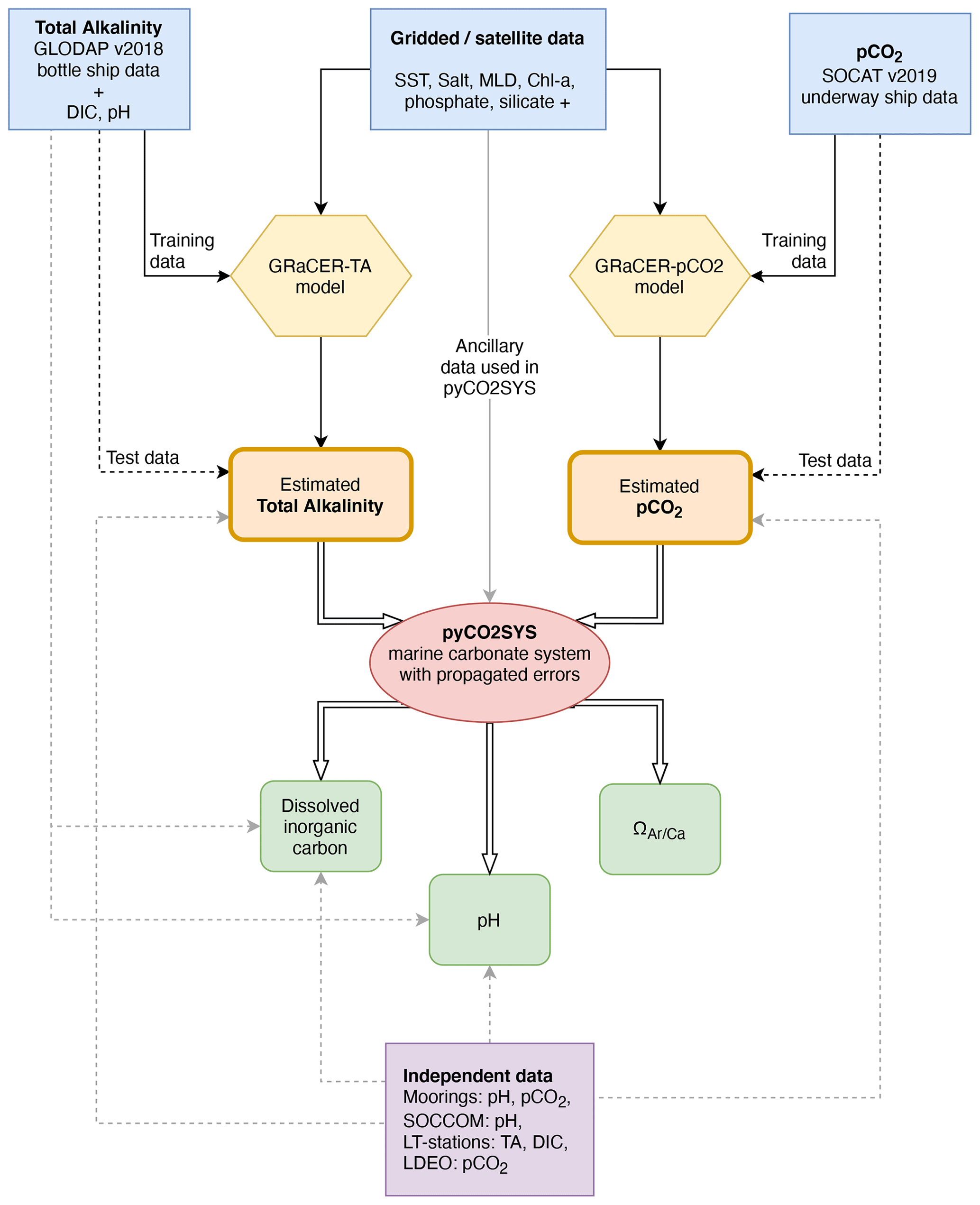
Figure 1 Schematic flow diagram showing the three steps required to reconstruct the surface ocean carbonate system. In the first step (yellow hexagons), the GRaCER (Geospatial Random Cluster Ensemble regression) method is used to develop statistical models for the observed TA (left) and pCO₂ (right) fields. In the second step (orange rectangles), these statistical models are used to extrapolate these two parameters over time and space using ancillary observations, primarily stemming from satellite observations. In the third step (red oval), the interpolated and extrapolated TA and pCO₂ fields are then used to compute the remaining parameters of the surface ocean carbonate system, namely DIC, pH, and the saturation state of seawater with regard to mineral CaCO₃, Ω. The output of steps two and three is the OceanSODA-ETHZ product. Also shown are the various data sets and data flows used in this study. The different lines indicate whether data are used for training (solid lines), testing (dashed lines), or output with an estimate of uncertainty, where independent test data are shown with gray dashed lines. The gridded/satellite data are summarized in Table 1. Independent test data are shown by the purple box. pyCO2SYS is the software used to solve the marine carbonate system and propagate uncertainties (Humphreys et al., 2020).

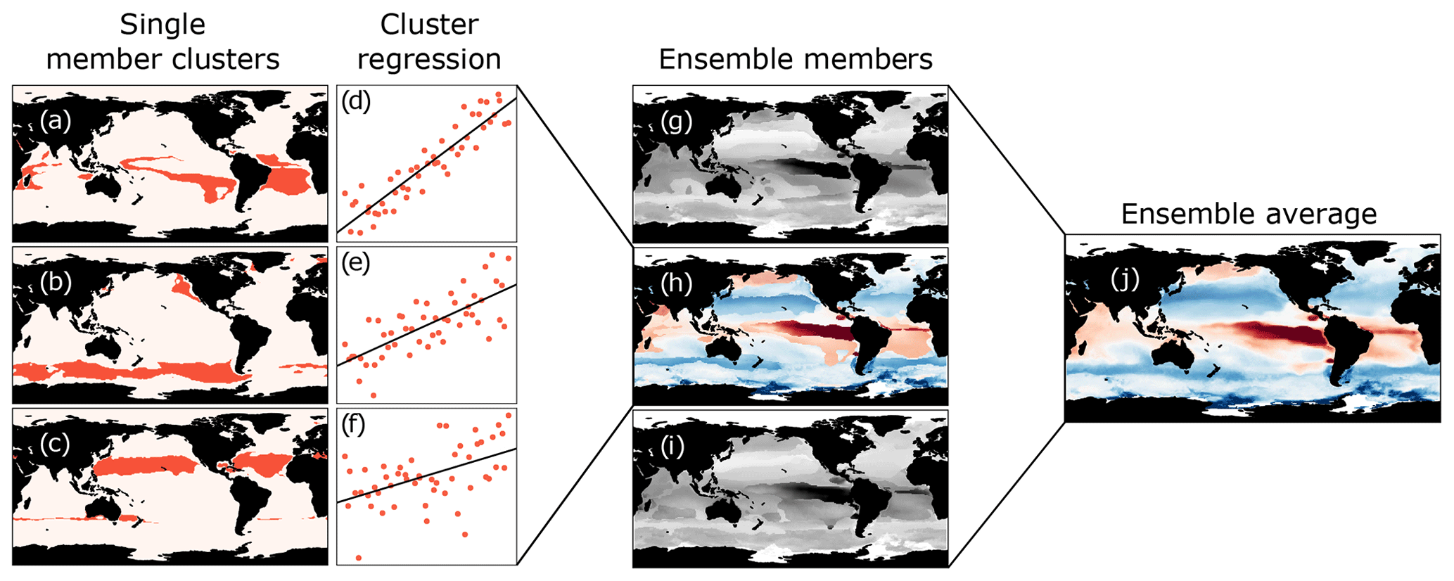
Figure 2 A schematic showing the steps used in the GRaCER method for a single month. Panels (a)–(c) show a subset of the clusters of a single ensemble member (h), with the adjacent scatter plots (d)–(f) showing the training data for each cluster and the linear regression models for that cluster (with toy data). Panels (g)–(i) show the ensemble member estimates for a subset of three members for pCO₂. Panel (j) shows the ensemble mean for all ensemble members, which includes ensemble members not shown in panels (g)–(i).

2.1 GRaCER algorithm

The GRaCER algorithm builds conceptually on a series of cluster-regression algorithms that have been successfully used for the interpolation and extrapolation of surface ocean pCO₂ (Sasse et al., 2013; Landschützer et al., 2013, 2016; Iida et al., 2015; Gregor et al., 2019). The main advantage of such a two-step approach is that the first clustering step organizes the variability regionally and temporally. This greatly enhances then the fidelity of the second step, i.e., the regression, as the size of the regression problem is reduced from the global domain to smaller, more homogeneous regions. A second advantage is that this clustering brings together regions with similar seasonality and similar co-variability with potential predictors, irrespective of the number of observations. The regression step explains the variability within each region over time and space dimensions, including interannual variability. Further, the clustering permits the regression to transfer information from spatially distant but geochemically similar regions, making the interpolation and extrapolation more robust in data-poor regions. The main innovation of the GRaCER algorithm relative to the previously used two-step approaches is its use of ensembles of cluster regressions, i.e., the generation of a whole series of clusters and corresponding regressions, which overcomes the boundary problems that are inherent in all two-step approaches.

For the clustering step, we use monthly climatological data of pCO₂ and TA and related parameters (Fig. 2a–c) to determine the main patterns of variability of the target variable and its co-variability with potential predictor variables. We opted for a clustering on climatological data rather than on the actual monthly data in order to clearly focus on the clustering step's role to isolate primarily regions with the same seasonal cycle. The alternative approach, i.e., to cluster on the monthly data, is also more prone to errors since the climatological distributions are better known than their month-to-month variations. Finally, clustering on monthly data would also take away signals from the regression step, which is actually better suited to capture the smaller level variations associated with the interannual variability and trends. The mini-batch K-means implementation in the Python scikit-learn package is used to perform the clustering due to its computational efficiency and scalability with large data sets (Pedregosa et al., 2011). A user-defined number of cluster centers are initiated, where cluster centers represent the mean of the points in a cluster. The K-means$++$ algorithm is used to initiate the cluster centers; it randomly selects the location of the first cluster center and then iteratively selects a best-guess location for the remaining cluster centers. Thereafter, the algorithm minimizes the distance between cluster centers and data points in the variable space. Once the clusters have been defined for the climatological domain, the co-located training data are assigned to the monthly clusters.

The regression is then performed individually for each of the clusters (Fig. 2d–f). The GRaCER method does not use a prescribed regression method – rather the appropriate algorithm for the particular use case is implemented. Importantly, the algorithm must be able to scale appropriately to the size of the problem. For example, the training data set for TA is $\mathrm{1}/\mathrm{20}$th of the size of the pCO₂ training data set; thus a more computationally expensive method can be used to predict TA.

The ensemble members are created by performing the cluster-regression step multiple times. Creating an ensemble is possible due to the fact that each clustering instance is slightly different (Fig. 2g–i). In practice, the spatial distribution of the clusters is similar; i.e., there is consistency in the typology of the clusters, particularly in regions where clusters are well defined, such as in the subtropical gyres and in the tropical eastern Pacific. However, there are regions that belong to different clusters; i.e., there is slight variance in the typology between ensemble members. The differences are due to the random initialization of the first cluster center in the K-means clustering step and the fact that clustering variables for some regions have weak gradients in spatial auto-correlation resulting in weak association with a cluster. In practice, this means that the locations of cluster boundaries vary between ensemble members; thus the ensemble mean does not have discrete boundaries (Fig. 2j).

2.2 Algorithm implementation

2.2.1 Total alkalinity

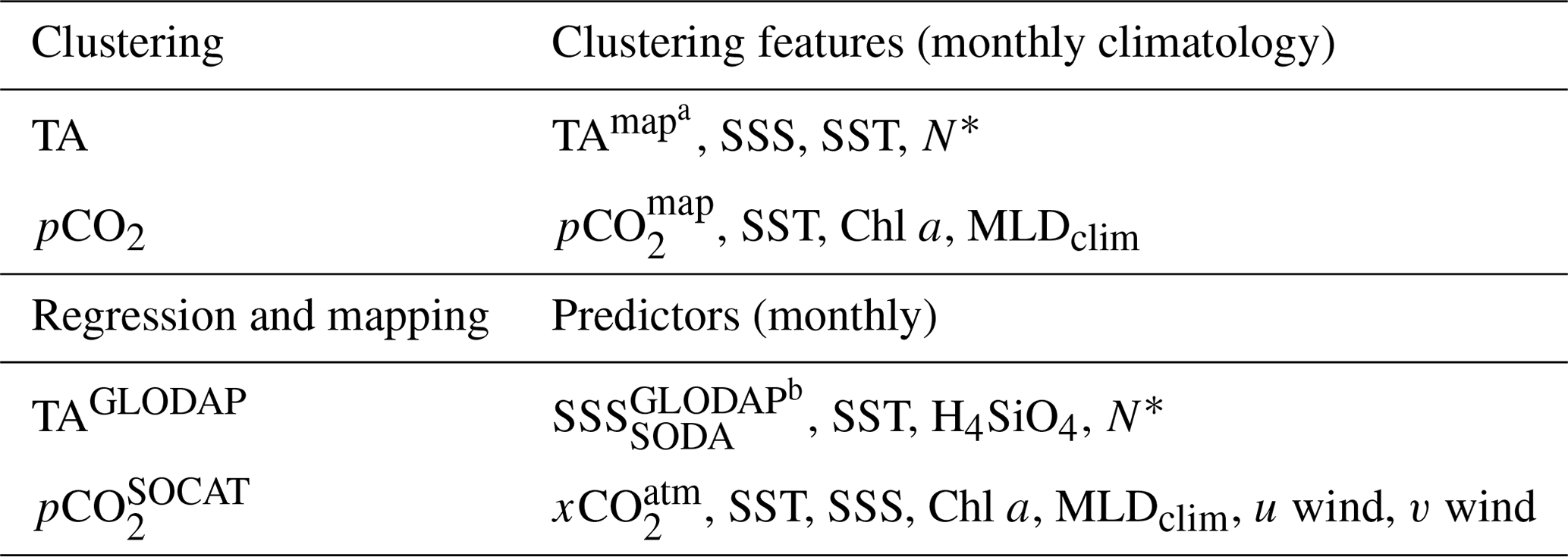
For the estimation of TA, we employ the support vector regression (SVR) method with 12 clusters and 16 ensemble members. The clustering is performed on climatological mean TA, sea-surface salinity (SSS), sea-surface temperature (SST), and nitrate (${\mathrm{NO}}_{\mathrm{3}}^{-}$; Table 1 and Sect. 2.3 below). The optimal variables on which clustering should be performed were selected by assessing the regression scores of each combination of variables following the methodology of Gregor et al. (2019). All data are standardized to the mean (μ) and standard deviation (σ) prior to clustering ($\frac{(x-\mathit{\mu })}{\mathit{\sigma }}$), after which TA is given 3 times the weight of the other variables.

A similar exhaustive search was used for determining the number of clusters. The number of ensemble members was chosen by the number above which there is no longer an increase in performance, analogous to the number of trees in a random forest. Test data are a subset of years spaced 3 years apart starting in 1985. We ensure that the models are not overfitted by selecting hyper-parameters using K-fold cross validation (further details are in Sect. A3).

To regress and map TA, we use SSS, SST, silicic acid (H₄SiO₄), and $N^{*}={\mathrm{NO}}_{\mathrm{3}}^{-}-\mathrm{16}\cdot {\mathrm{PO}}_{\mathrm{4}}^{\mathrm{3}-}$ (nitrogen excess relative to phosphate in terms of the Redfield N : P ratio simplified from Gruber and Sarmiento, 1997) as predictors. Our choice of SSS and SST as predictors is easily justified by these two variables accounting for the majority of TA variability (Lee et al., 2006; Carter et al., 2018). The addition of H₄SiO₄ and N^* as predictors is to account for seasonal changes in primary production that has an impact on TA (Wolf-Gladrow et al., 2007; Carter et al., 2018). Further, N^* expresses the zonal differences between and within the large ocean basins better than using simply ${\mathrm{NO}}_{\mathrm{3}}^{-}$ or ${\mathrm{PO}}_{\mathrm{4}}^{\mathrm{3}-}$ – an important consideration, since coordinates (i.e., latitude and longitude) are not included in our set of predictors.

2.2.2 Partial pressure of CO₂

For the estimation of pCO₂, we use two regression methods, i.e., GBDTs (gradient boosted decision trees) and FFNNv2 (feed-forward neural network). These are implemented with 21 clusters and 16 ensemble members (eight each). The number of clusters is at the upper end of the range compared with the number of clusters used by the MPI-SOMFFN or CSIR-ML6 methods. However, testing has shown that additional clusters are required to account for the additional complexity by our inclusion of data from the coastal, Arctic, and Mediterranean seas.

Clustering is performed on climatological values of pCO₂, SST, mixed-layer depth (MLD), and chlorophyll a, with additional weighting given to pCO₂. As with TA, all variables are standardized prior to clustering with $\frac{(x-\mathit{\mu })}{\mathit{\sigma }}$, after which pCO₂ is multiplied by 3 to give it stronger weighting.

Details of the regression method and of the hyper-parameter selection are given in Sect. A3. Test data are selected as every fifth year starting in 1985, and validation data for early stopping are selected using the same approach starting in 1987, where the latter are used for early stopping to reduce overfitting and keep model complexity within bounds.

The regression and mapping is performed with the following variables as predictors: SST, SSS, the logarithm of chlorophyll a, the logarithm of mixed-layer depth, the meridional and zonal components of the surface winds, the sine and cosine of $\frac{\text{day of year}\cdot \mathit{\pi }}{\mathrm{365}\cdot \mathrm{180}}$, and the atmospheric dry-air mixing ratio (xCO₂). These predictors are the same as used by Gregor et al. (2019), and various combinations of these methods have been used by previous approaches (Landschützer et al., 2014; Denvil-Sommer et al., 2019).

It is important to note that the predictors are proxies for the spatiotemporal changes in pCO₂ and do not necessarily explain the physical mechanism by which changes in pCO₂ are driven. For example, an increase in sea-surface temperature in the subtropics results in an increase in pCO₂ as shown by Takahashi et al. (1993) and Lefèvre and Taylor (2002). In contrast, surface warming in the Southern Ocean can be a proxy for stratification that reduces outcropping of high-CO₂ waters (Landschützer et al., 2015; Gregor et al., 2018). Similarly, changes in SSS and MLD also capture the distribution and processes that drive changes in surface pCO₂, such as stratification and mixing. However, the climatological MLD product used here does not capture interannual variability in stratification and mixing. We thus include the two surface wind components that, along with SST, are a proxy for wind-driven mixing and upwelling. Chlorophyll is also an important driver of pCO₂ on a local scale, particularly in the high-latitude regions where high primary productivity results in rapid uptake of pCO₂ (Bakker et al., 2008; Gregor et al., 2018). Lastly, xCO₂ is included to account for the close tracking of oceanic pCO₂ to atmospheric CO₂ concentrations (Bates et al., 2014).

2.3 Data

Data are used to develop the two-step GRaCER model, i.e., clustering and regression, and to evaluate the estimates. Table 1 provides an overview of all data employed and the purposes for which they are used, and Table 2 shows the corresponding source of the data. We describe each data set by parameter and use.

Table 1 Variables used as the clustering features and predictor variables for regression. Details about these data are given in the text. Note that clustering features are all resampled to monthly climatologies. ^a TA^map is the exception where a quasi-annual mean is used. The first column for regression shows the target variable. All machine learning models use the same variables to train and predict the final estimates with the exception of ^b SSS, where ungridded GLODAP data are used to train and SODA salinity is used to predict. All other references to SSS refer to the gridded SODA product.

Bakker et al. (2016)Landschützer et al. (2016)Rödenbeck et al. (2014)Denvil-Sommer et al. (2019)Takahashi et al. (2014)Olsen et al. (2016)Lauvset et al. (2016)Good et al. (2020)Carton et al. (2018)Holte et al. (2017)Dlugokencky et al. (2019)Maritorena et al. (2010)Boyer et al. (2013)

Table 2 Data sources used in this study.

2.3.1 Data for clustering

For the clustering of TA, we used the mapped product of total alkalinity (TA_map) from the GLODAPv2 (Lauvset et al., 2016). This product represents a quasi-annual mean as it was generated without consideration of the seasonal cycle. We repeat this quasi-annual mean TA to create a monthly data set over which clustering can be performed. We thus assume that the spatial variability of TA is larger than the seasonal variability. This is backed by Takahashi et al. (2014) and Broullón et al. (2018), who found that the seasonal variability of TA for the majority of the ocean was more than a factor of 10 smaller than the spatial variability.

For the clustering step of pCO₂, we use four data-based products resampled and gridded to a monthly by $\mathrm{1}{}^{\circ }\times \mathrm{1}{}^{\circ }$ resolution ($p{\mathrm{CO}}_{\mathrm{2}}^{\mathrm{map}}$), namely LDEO by Takahashi et al. (2014), MPI-SOMFFN by Landschützer et al. (2016), Jena-MLS by Rödenbeck et al. (2014), and CMEMS-FFNNv2 by Denvil-Sommer et al. (2019). It may seem tautological to use other machine learning estimates, but these data are just used to create regional clusters; i.e., they are not used in the regression step. Relative to previous two-step approaches (Landschützer et al., 2016; Denvil-Sommer et al., 2019), which used just the LDEO product, we expanded on this by including three more estimates. In doing so, we make the implicit assumption that this ensemble of estimates is a better representation of the pCO₂ monthly climatology than the LDEO climatology alone.

SSS is from the Simple Ocean Data Assimilation (SODA) analysis (Carton et al., 2018) and SST from the Operational Sea Surface Temperature and Sea Ice Analysis (OSTIA) product (Good et al., 2019, 2020). N^* is calculated using monthly climatologies of ${\mathrm{NO}}_{\mathrm{3}}^{-}$ and ${\mathrm{PO}}_{\mathrm{4}}^{\mathrm{3}-}$ from the World Ocean Atlas updated in 2018 (Boyer et al., 2013). We use the monthly climatology of density-based mixed-layer depth (MLD) from Holte et al. (2017) that is estimated from Argo float profiles. The MLD data product merges monthly estimates of MLD from multiple years but is averaged into a climatology due to the paucity of data on an annual scale. A two-dimensional moving average filter is applied to the MLD to interpolate missing data and remove the noise introduced by interannual and sub-monthly variability.

Chlorophyll a (Chl a) is from the GlobColour project where a monthly climatology is calculated for the period from 1998 through 2018 (Maritorena et al., 2010). The missing data in the high latitudes during winter are filled with a 0.3 mg m³, which is roughly the 20th percentile of global chlorophyll a. Lastly, we take the log transformation (base 10) of Chl a to convert the log-like distribution of Chl a to a normal distribution for improved performance in the gradient descent algorithm of the FFNNv2.

2.3.2 Data for regression and mapping

For the regression step of TA, the bottle measurements from the GLODAP v2 product are used as the target variable (Olsen et al., 2019). Following Lee et al. (2006), we select data shallower than 20 m in latitudes lower than 30^∘ and shallower than 30 m at higher latitudes. We do not exclude measurements taken in nearshore and coastal environments as was previously done. The quality of TA measurements was historically not as rigorous as the SOCAT pCO₂ data due to the lack of reference standards before the mid-1990s (Bockmon and Dickson, 2015). However, most of the biases in the cruises were corrected based on calibration to deep samples, where it is assumed that interannual TA variability is negligible relative to the magnitude of the bias (Olsen et al., 2019). These bias corrections amount to ± 5 µmol kg⁻¹ on average.

For the regression of pCO₂, we use SOCAT v2019 where only data with a SOCAT cruise quality flag of A to D and a World Ocean Circulation Experiment (WOCE) quality flag of 2 are used. As is the case for TA, we do not exclude data from coastal and nearshore environments. The fugacity of CO₂ (fCO₂) reported in SOCAT v2019 is converted to pCO₂ using

$$\begin{array}{}\text{(1)}& p{\mathrm{CO}}_{\mathrm{2}}=f{\mathrm{CO}}_{\mathrm{2}}\cdot \exp \left(P_{\mathrm{atm}}^{\mathrm{surf}}\cdot {\displaystyle \frac{B+\mathrm{2}\cdot \mathit{\delta }}{R\cdot T^{\mathrm{SOCAT}}}}\right),\end{array}$$

where P is atmospheric pressure at sea level from the ERA5 reanalysis product (Hersbach, 2018). B and δ are virial coefficients, R is the gas constant, and T^SOCAT is the ship intake temperature in ^∘C (Dickson et al., 2007). In exploratory work for this study, we tested predicting $\mathrm{\Delta }p{\mathrm{CO}}_{\mathrm{2}}=p{\mathrm{CO}}_{\mathrm{2}}^{\mathrm{atm}}-p{\mathrm{CO}}_{\mathrm{2}}$ instead of just pCO₂ but found that this did not produce credible results; for a more in-depth discussion see Sect. A2.

The discrete measurements of pCO₂ and TA are resampled on a monthly grid (January 1985 through December 2018) with a spatial resolution of $\mathrm{1}{}^{\circ }\times \mathrm{1}{}^{\circ }$ to match the predictors used in the mapping step.

Finally, outliers are removed from gridded $p{\mathrm{CO}}_{\mathrm{2}}^{\mathrm{SOCAT}}$ using the methods described in Sect. A1. In total, 2425 points are removed from the gridded $p{\mathrm{CO}}_{\mathrm{2}}^{\mathrm{SOCAT}}$ using these outlier removal approaches, equivalent to 0.85 % of the original gridded data.

We use sea-surface temperature from OSTIA for both TA and pCO₂ regression (Good et al., 2020). The TA model is trained using in situ salinity from GLODAP v2, but salinity from SODA v4.3.2 is used for the mapping step (Olsen et al., 2019; Carton et al., 2018). The N^* and H₄SiO₄ are the same as used in the clustering step but are repeated for the number of years. Similarly, the mixed-layer depth climatology described in Sect. 2.3.1 is repeated for each year. We use the global mean of the mole fraction of CO₂ for the marine boundary layer ($x{\mathrm{CO}}_{\mathrm{2}}^{\mathrm{mbl}}$) as a predictor in the regression, as the correction for water vapor pressure may otherwise introduce co-variance with other predictors (i.e., SST, SSS). Missing data in the monthly GlobColour chlorophyll a product are filled with climatological data described in Sect. 2.3.1. The meridional and zonal components of the surface winds are averaged from the hourly output from the ERA5 reanalysis (Hersbach, 2018).

2.3.3 Evaluation variables

The machine learning estimates of TA, pCO₂, and the computed DIC and pH are evaluated against data that are not used in the training or mapping step.

For DIC and pH, we use the directly measured data from GLODAP v2.2019 (Olsen et al., 2019). Bockmon and Dickson (2015) report a measurement error of ± 5 µmol kg⁻¹ for GLODAP DIC in an inter-laboratory comparison. Olsen et al. (2019) estimate the measurement error for pH to be 0.01. To be consistent with TA, we select data shallower than 20 m in latitudes lower than 30^∘ and shallower than 30 m at higher latitudes and resampled the data to monthly by $\mathrm{1}{}^{\circ }\times \mathrm{1}{}^{\circ }$.

Three long-term time series stations are used to provide direct independent comparisons for DIC and TA, namely the Hawaii Ocean Time-series at 22.57^∘ N, 158^∘ W (HOT, Dore et al., 2009); the Bermuda Atlantic Time-series Study at 32^∘ N, 64^∘ W (BATS, Bates and Peters, 2007); and the Irminger station in the high northern Atlantic (64.3^∘ N, 28^∘ W, Olafsson et al., 2010, only for DIC). The accuracy for these measurements is reported to be below 2 µmol kg⁻¹ for DIC and ∼ 4 µmol kg⁻¹ for TA for all stations. We use the same depth constraints for the long-term stations as for GLODAP, explained in the paragraph above. pCO₂ is also calculated from DIC and TA for HOT and BATS to provide an additional constraint.

Data present in the Lamont-Doherty Earth Observatory pCO₂ data set but not in SOCAT are used to independently compare pCO₂ (Takahashi et al., 2020). Takahashi et al. (2020) report an error estimate of ±2.5 µatm, but it must be added that some of the data unique to LDEO may be excluded from SOCAT due to stricter quality control criteria for the latter; thus errors for the LDEO data are expected to be larger (Bakker et al., 2016).

Finally, we include Argo float measurements of pH from the Southern Ocean Carbon and Climate Observations and Modeling project (SOCCOM) (Johnson et al., 2017; Williams et al., 2017). Johnson et al. (2016) report a mean uncertainty of ± 0.019 for pH for the entire water column, though this is likely higher for the upper 30 m as the authors report lower errors for estimates below 50 m.

2.4 Computation of DIC, pH, and Ω

The remaining parameters of the marine carbonate system, i.e., DIC, pH, and Ω, are computed using the Python version of CO2SYS (Humphreys et al., 2020) originally developed by Lewis et al. (1998). In addition to pCO₂ and TA, CO2SYS requires the input of sea-surface temperature, sea-surface salinity, pressure (assumed 0 dbar at the surface), ${\mathrm{PO}}_{\mathrm{4}}^{\mathrm{3}-}$, and H₄SiO₄. We use the same data sources described in Sect. 2.3.2 and Table 1. Climatologies of H₄SiO₄ and ${\mathrm{PO}}_{\mathrm{4}}^{\mathrm{3}-}$ are repeated for each year, thus assuming no interannual variability. The impact of this assumption is minimal (≪ 2 µmol kg⁻¹), as can be shown by varying these nutrients over seasonal cycle. The dissociation constants by Dickson et al. (1990) for $K_{{\mathrm{HSO}}_{\mathrm{4}}}$ and the total boron–salinity relationship by Uppström (1974) were used, as recommended by Orr et al. (2015) and Raimondi et al. (2019). For further details on the calculation and the full description of the marine carbonate system, see Dickson et al. (2007).

An important consideration in these calculations is the internal consistency of the marine carbonate system, i.e., the error due to uncertainties in the equations and coefficients that describe the marine carbonate system. Raimondi et al. (2019) pointed out that the pCO₂–TA pair has the lowest error in the calculation of pH (0.003 ± 0.008 pH units) using the dissociation constants by Mehrbach et al. (1973) as refitted by Dickson and Millero (1987). However, using the same pair and the same dissociation constants resulted in an estimate of Ω with respect to aragonite that is very different from that computed using the DIC–TA pair. But since Raimondi et al. (2019) lacked direct measurements of Ω, it remains unclear which pair is actually better for Ω. We cannot resolve this here but need to acknowledge that this inconsistency adds some additional uncertainty to our computed Ω values.

3 Uncertainty assessment

Any application of our data product requires a firm understanding of the errors and uncertainties associated with each of the reported parameters of the surface ocean carbonate system. We first discuss the errors and uncertainties associated with the statistically modeled quantities TA and pCO₂ and then those with the computed parameters DIC, pH, and Ω. Then, we will compare these propagated uncertainties with the uncertainty of the computed DIC and pH by comparing these values with in situ observations. This provides a strong check on our ability to establish a full uncertainty budget. Here, we use the term “uncertainty” to characterize the range of values within which the true value is asserted to lie with some level of confidence. The term “error” is used in two ways: first, as a process that leads to deviations between the measurement and the true value and, second, as an estimate quantifiable against a known value. For the purpose of our analysis here, we consider the training data sets for TA and pCO₂ as such known values; i.e., we assume that these observations are unbiased. This can be justified on the basis of their having undergone extensive secondary quality control.

3.1 Sources of errors for TA and pCO₂

We identify three sources of errors that contribute to the total uncertainty for pCO₂ and TA, namely the uncertainty stemming from the measurement (M), representation (R), and prediction (P) errors. Assuming independence of the three error sources, the total uncertainty (E) for the TA and pCO₂ estimates can thus be expressed as the root of the squared sum of the uncertainties from the three error sources:

$$\begin{array}{}\text{(2)}& E=\sqrt{M^{\mathrm{2}}+R^{\mathrm{2}}+P^{\mathrm{2}}}.\end{array}$$

The measurement error reflects the combination of potential biases (systematic errors) from sampling and measurement as well as random errors associated with sampling and the imprecise nature of the measurement system. Since both TA and pCO₂ are being measured against certified reference materials and have undergone extensive secondary quality control, we assume that they have no systematic error, i.e., that their bias is zero. We also assume the sampling error to be small, so that the uncertainty M associated with the measurement error can be well approximated by the precision of the employed measurement methodology (Dickson et al., 2007).

The representation error, R, is a result of the fact that we develop our statistical model (GRaCER) on a grid that is in many places coarser in time and space than the typical scales of variability of TA and pCO₂. As a result, any given observation may not be representative for the $\mathrm{1}{}^{\circ }\times \mathrm{1}{}^{\circ }$ monthly grid cell used as a basis for our regression, leading to a bias in the estimated mean relative to the true spatial and temporal mean. This problem is particularly severe if the number of samples within any grid cell is low and the spatiotemporal variability is high. This is often the case. For example, more than 90 % of the data in the monthly gridded pCO₂ product are based on a single day of sampling within the month. The situation is more dire for TA, for which there are 10-fold fewer observations than pCO₂. Since we are lacking full knowledge of the spatial and temporal variability of TA and pCO₂, we cannot fully quantify the representation error. Instead, we approximate it using the few regions where we have sufficient observations or then using closely related parameters for which we have more observations. For simplicity, we make the assumption that the uncertainty associated with this error is, on a global average, normally distributed with a bias of 0.

The uncertainty associated with the prediction error, P, is determined by the test scores from the evaluation of the statistical model vis-à-vis the independent test data. The test scores describe the error incurred in the prediction of the subset of data that are not used in the training step. This error includes also the propagated uncertainty associated with the predictor variables.

We summarize these uncertainties with mean biases ($\frac{{\sum }_{i=\mathrm{1}}^N({\widehat{y}}_i-y_i)}{N}$) and root mean squared error (RMSE, $\sqrt{\frac{{\sum }_{i=\mathrm{1}}^N({\widehat{y}}_i-y_i{)}^{\mathrm{2}}}{N}}$), where y is the target value, $\widehat{y}$ is the predicted value, and N is the number of observations. We separate the coastal and open-ocean regions using the COastal Segmentation and related CATchments (COSCATs) mask (Laruelle et al., 2013) in order to reflect their very different levels of spatiotemporal variability.

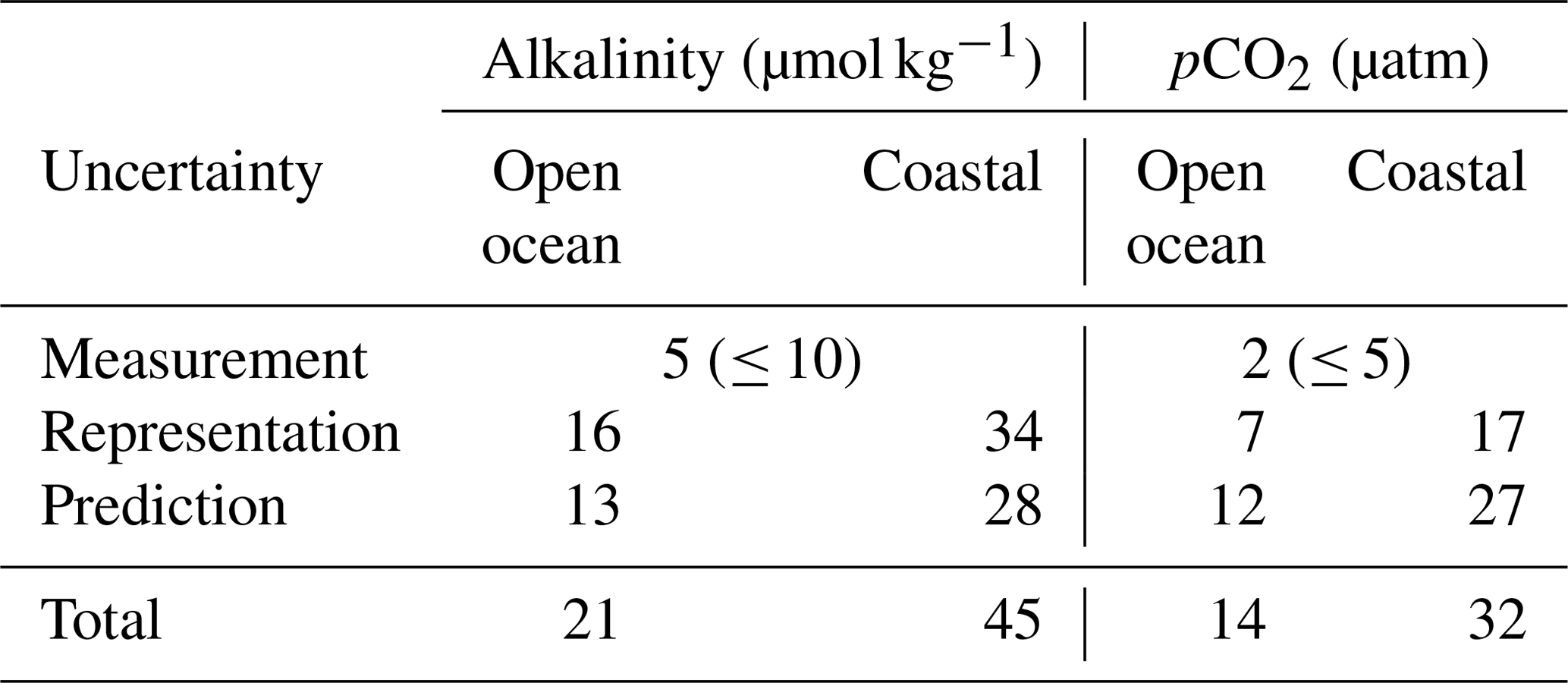
Table 3 Summary of the uncertainties of total alkalinity and pCO₂ from the different error sources (see Table 2) separately evaluated for the open ocean and for coastal regions (defined by the COSCATs regions, Laruelle et al., 2013). See text for details on how the different sources were quantified.

3.1.1 Uncertainty for total alkalinity

We adopt an uncertainty M associated with the measurement error of TA of ± 5 µmol kg⁻¹ based on the laboratory intercomparison by Bockmon and Dickson (2015). This is only half the accuracy of ± 10 µmol kg⁻¹ or 0.5 % reported by GLODAPv2 (Olsen et al., 2019). We consider this to be an overly conservative estimate, since Bockmon and Dickson (2015) pointed out that the majority of the laboratories involved in the round-robin exercise achieved an accuracy of better than ± 5 µmol kg⁻¹. We thus opted for this lower value that is more representative of the majority of the data.

Owing to the sparseness of the TA observations, we cannot estimate the uncertainty R associated with the representation error directly. Instead, we use the high correlation between TA and salinity. This permits us to determine the representation error for TA indirectly from an estimate of the representation error of sea-surface salinity. Concretely, we compare the test RMSE of TA predicted with GLODAPv2's in situ salinity with the RMSE of TA predicted with the satellite-based SODA salinity (see Table 1). Since the latter salinity is supposed to reflect the true time–space average over each grid cell, the difference between these two salinities is a direct estimate of the uncertainty associated with the representation error for salinity. Consequently, the difference in TA from these two estimates is an estimate of the uncertainty associated with the representation error for TA. The resulting estimates for the open and coastal ocean are summarized in Table 3.

The uncertainty P associated with the prediction error is based on the model's RMSE score calculated from test data and is listed in Table 3 and Fig. 3a. The global mean prediction error for the open ocean amounts to 13 µmol kg⁻¹, with some regional differences. The prediction error is more than twice this number in the coastal regions, i.e., 28 µmol kg⁻¹ (coastal regions are defined by the COSCATs regions, Laruelle et al., 2013). We find especially high prediction errors, for example, in the highly dynamic Amazon outflow region or the Gulf of Maine in the northwestern Atlantic. However, in such regions, one can expect that part of the high prediction error is actually stemming from a representation error, as we are not using directly co-measured variables when we train our regression model. In Fig. A2, we show the spatially and climatologically mapped test errors for TA in Fig. A2 using the GRaCER approach.

While the global bias of the TA product of OceanSODA-ETHZ is near zero (0.5 µmol kg⁻¹), confirming our assumption about the unbiased nature of our prediction error, this is not the case regionally. For example, OceanSODA-ETHZ tends to consistently overestimate TA in the southeastern Atlantic and underestimate TA in the southern Indian Ocean (Fig. 3b). A seasonal breakdown of the biases into DJF and JJA reveals that the winter period of each hemisphere has biases in the high latitudes, though the paucity of data means that we can place less weight on this finding.

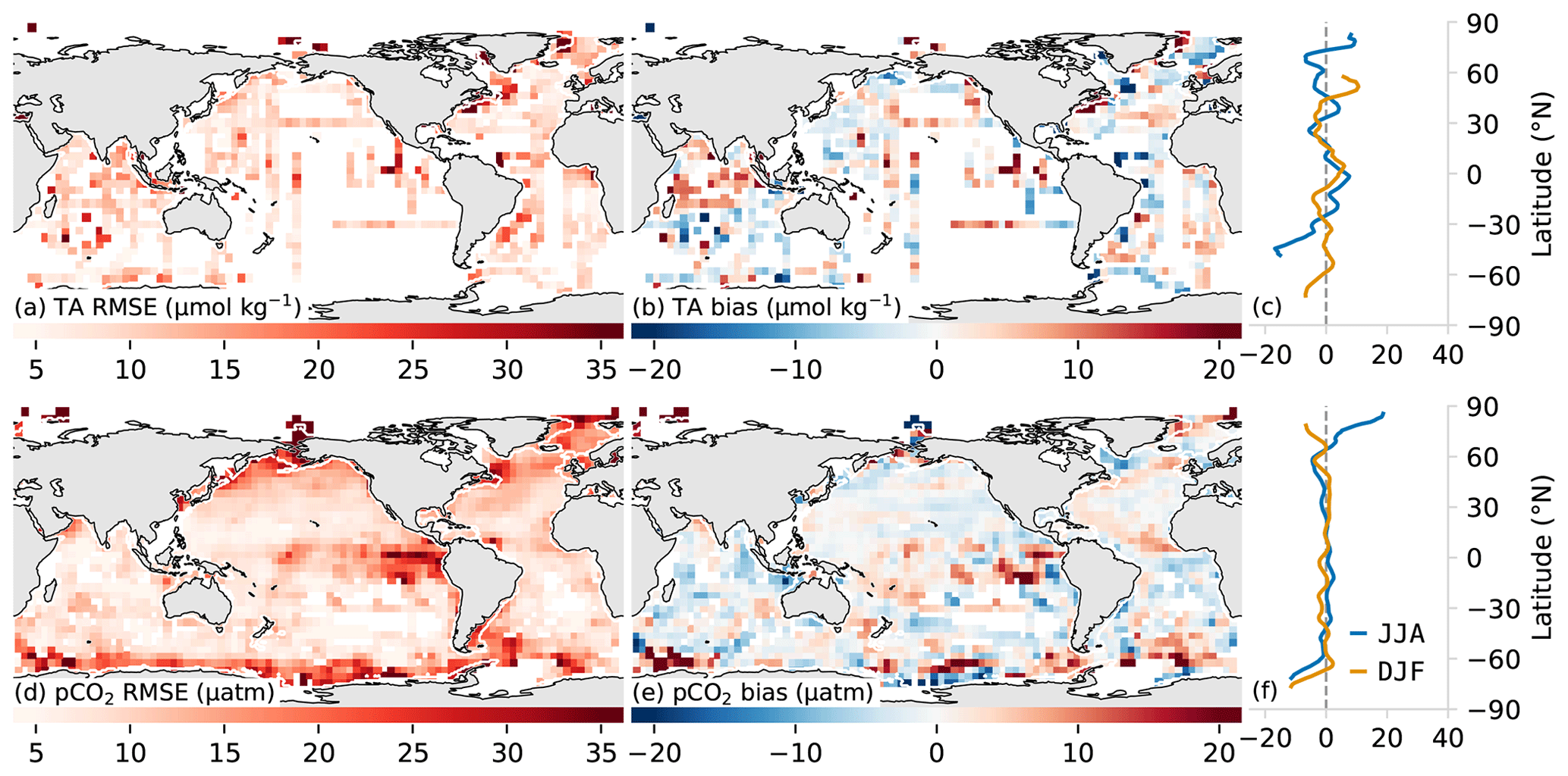
Figure 3 Test metrics for total alkalinity (a, b) and pCO₂ (c, d). The left-hand column (a, d) shows the root mean squared error (RMSE) compared with the target data. Similarly, the middle column (b, e) shows bias compared to the respective training data sets (GLODAP v2.2019 and SOCAT v2019). The right-hand column shows the zonally averaged biases for June, July, and August (JJA, blue) and December, January, and February (DJF, orange). A 2D spatial convolution was first applied to the $\mathrm{1}{}^{\circ }\times \mathrm{1}{}^{\circ }$ pixels to make regional patterns in the biases and RMSE clearer, and data were then aggregated into $\mathrm{4}{}^{\circ }\times \mathrm{4}{}^{\circ }$ pixels for clearer visualization.

A good check on the model prediction error is provided by comparing the estimated TA against independent observations. To this end, we use data from the Hawaii Ocean Time-series (HOT), the Bermuda Atlantic Time-series Study (BATS), and the Irminger station shown in Fig. 4a, b, e, f, i, and j and Table 4. For the period 1990–2018, the bias for BATS is 3 µmol kg⁻¹ and for HOT −2 µmol kg⁻¹, indicating that the method captures the overall structure and variability of TA well at these subtropical stations. Further, the mean seasonal cycle is relatively well represented at HOT and BATS, being within 1 standard deviation of the interannual variability when averaged as a climatology (Fig. 4b, f). However, the results are not as good for the Irminger station in the Atlantic high latitudes (∼ 65^∘ N), where OceanSODA-ETHZ has a large negative bias (−10 µmol kg⁻¹) when compared to TA computed from the observed pCO₂ and DIC. OceanSODA-ETHZ also overestimates the weak seasonal cycle of TA at the Irminger station, contributing to the large bias that is particularly strong from December to May. The RMSE at Irminger station is 15 µmol kg⁻¹, less than 5 µmol kg⁻¹ larger than the RMSE for HOT and BATS stations (10 µmol kg⁻¹ respectively) owing to the small interannual and seasonal amplitude at Irminger. The RMSEs are thus smaller than the mean prediction error (13 µmol kg⁻¹) at the subtropical stations yet exceed this mean estimate at the high-latitude station.

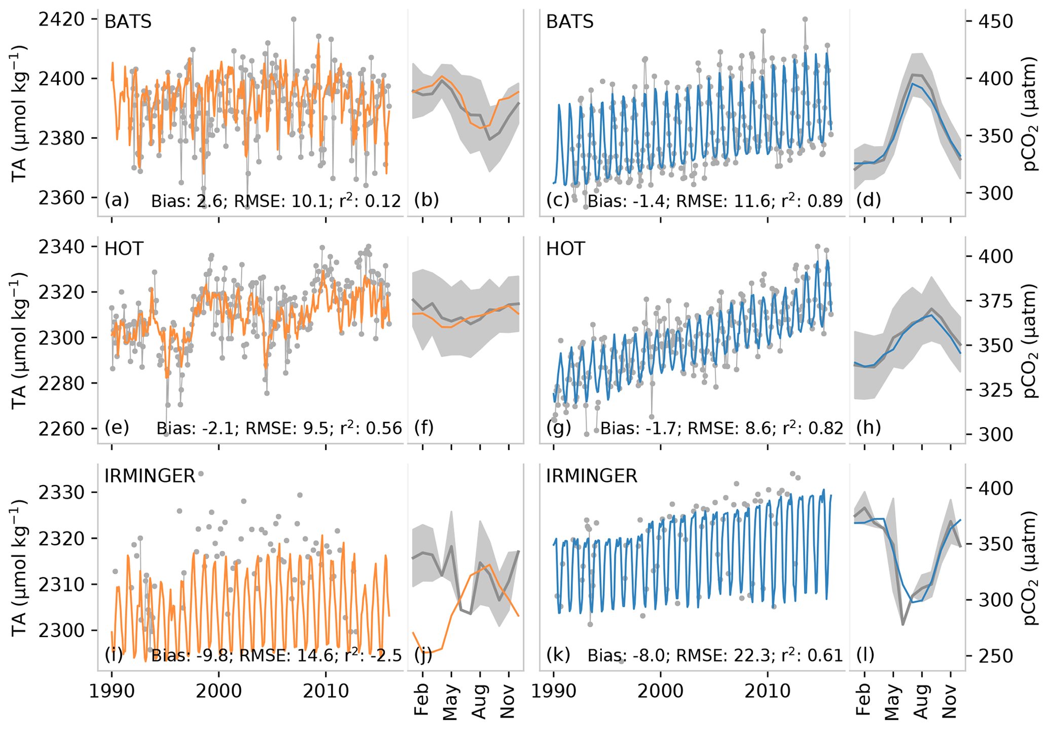
Figure 4 A comparison of a subset of measurements from long-term observation stations (gray) with predicted total alkalinity (TA) (a, b, e, f, i, j) and partial pressure of CO₂ (pCO₂) (c, d, g ,h, k, l). The top row (a–d) shows data for the Bermuda Ocean Time-series Study (BATS), the middle row (e–h) shows data for the Hawaii Ocean Time-series (HOT), and the bottom row (i, l) shows data for the Irminger station. The narrow panels show the average of the seasonal climatology for the time series. The gray shading shows the standard deviation of the observations for the period 1990 to 2018, while the orange/blue lines show the average estimate. TA for the Irminger station is calculated from pCO₂ and DIC, and pCO₂ is calculated for BATS and HOT using DIC and TA, as described in Sect. 2.4.

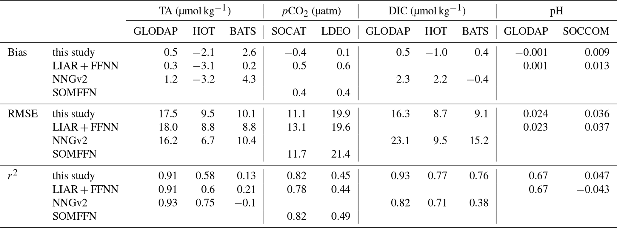
Table 4 Comparison of training and independent data sources with various methods for the open-ocean region using the COSCATs coastal mask by Laruelle et al. (2013). GLODAP refers to the GLODAP v2 2019 data (Olsen et al., 2019), HOT refers to the Hawaii Ocean Time-series (Dore et al., 2009), BATS refers to Bermuda Atlantic Time-series Study (Bates and Peters, 2007), SOCAT is the 2019 version of the Surface Ocean Carbon Atlas (Bakker et al., 2016), LDEO is the Lamont-Doherty Earth Observatory pCO₂ data set for points not present in SOCAT (Takahashi et al., 2020), and SOCCOM is the pH measured by autonomous floats from the Southern Ocean Carbon and Climate Observations and Modeling project (Johnson et al., 2016). Statistical outliers were excluded in the calculation of LDEO RMSE. OS-ETHZ is the OceanSODA-ETHZ data from this study, NNGv2 is from Broullón et al. (2018), LIARv2 from Carter et al. (2018), CMEMS-FFNNv2 from Denvil-Sommer et al. (2019), and SOMFFN from Landschützer et al. (2016). NNGv2 and LIARv2 predictions are made with SODA salinity and OSTIA sea-surface temperature, resulting in different estimates to the original publications (Broullón et al., 2018; Carter et al., 2018). Note that the full data set is used for OceanSODA-ETHZ, unlike Table 3, which presents the errors for test years.

3.1.2 Uncertainty for pCO₂

For the uncertainty M associated with the measurement error of pCO₂, we adopt a value of ±2 µatm. This reflects the fact that 80 % of the data we have used from SOCAT (flags A and B) have a precision better than that number and an accuracy of similar magnitude. The remaining data we used (SOCAT flags C and D) have a measurement precision and accuracy of less than ±5 µatm.

We estimate the uncertainty R associated with the representation error of pCO₂ on the basis of a spatiotemporal gradient analysis. To this end, we compare the pCO₂ in our regular grid that has a resolution of $\mathrm{1}{}^{\circ }\times \mathrm{1}{}^{\circ }$ by 1 month, with the pCO₂ binned to a grid with twice this resolution, i.e., $\mathrm{0.5}{}^{\circ }\times \mathrm{0.5}{}^{\circ }$ by 15 d. In regions with high spatiotemporal coverage, the difference in the average of adjacent grid cells represents the potential change that can occur within the coarser $\mathrm{1}{}^{\circ }\times \mathrm{1}{}^{\circ }$ by a 1-month grid cell. The spatial and temporal gradients are calculated separately, and we take the average of these two elements. Using this analysis, we estimate a representation error of our pCO₂ estimates of 7 and 17 µatm for the open and coastal ocean respectively (Table 3).

From the RMSE of our test data, we estimate an uncertainty P associated with the prediction error of pCO₂ of 12 µatm for the open ocean and 28 µatm for the coastal ocean (Table 3). Within the open ocean (Fig. 3e), the eastern tropical Pacific has the highest RMSE, but this is also the region with the highest variance in the observations. The strong horizontal gradients in the region increase the errors, particularly at cluster boundaries. The high RMSE for the coastal region stems primarily from coastal Antarctica as well as some coastal regions in the higher latitudes of the Northern Hemisphere. The former is due to large uncertainties in pCO₂ during the summer months when retreating ice and ensuing rapid net primary production result in large gradients (Bakker et al., 2008). The climatologically mapped errors for pCO₂ are shown in Fig. A2b and d, created by mapping the test errors to the clusters and averaged over the ensemble.

The comparison between the regression estimated and observed pCO₂ reveals regional biases (Fig. 3e), despite the global bias being close to zero (−0.37 µatm). Some of the highest biases are found, again, in the eastern tropical Pacific, where strong horizontal gradients drive the observed juxtaposed biases. The large negative biases in winter in the Southern Ocean are likely driven by the paucity of data in this region (Gregor et al., 2019; Gray et al., 2018; Bushinsky et al., 2019).

The time series comparisons show that the seasonal cycle is well represented at BATS and HOT with r² scores of 0.89 and 0.82 respectively (Fig. 4d, h). Low biases (<2 µatm in absolute terms) further demonstrate that pCO₂ estimates are reliable in the subtropics. The seasonal cycle is also well captured at the Irminger station in the high latitudes, but a lower r² score and larger bias (−8.0 µmol kg⁻¹) allude to the dampened amplitude of the seasonal cycle particularly in the winter months (Fig. 4).

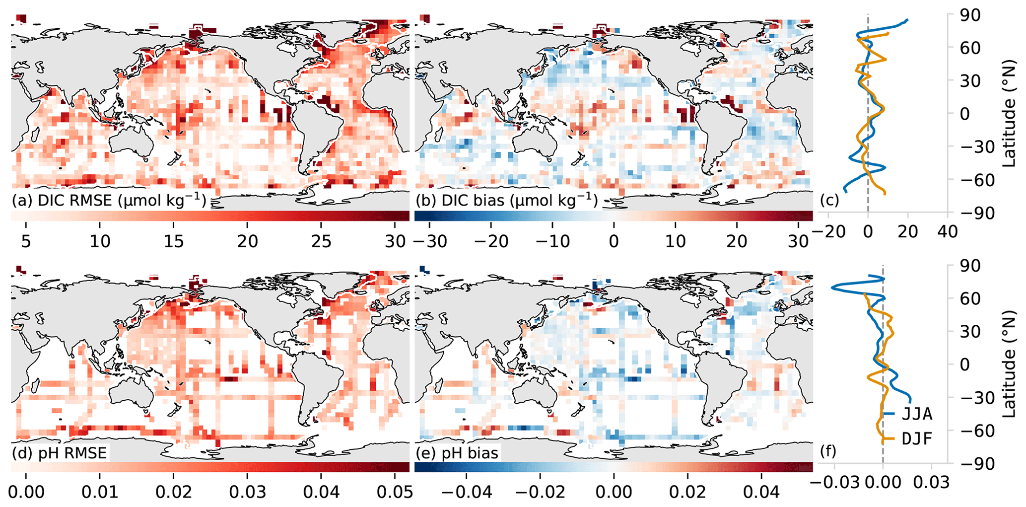
Figure 5 Root mean squared error (RMSE – a, d) and biases (b, c, e, f) for dissolved inorganic carbon (DIC, a, b, c) and pH (d, e, f) compared with in situ GLODAP v2.2019 data. The two subplots in the rightmost column compare the zonally averaged bias for JJA and DJF. Data were processed for plotting as described in Sect. 4.

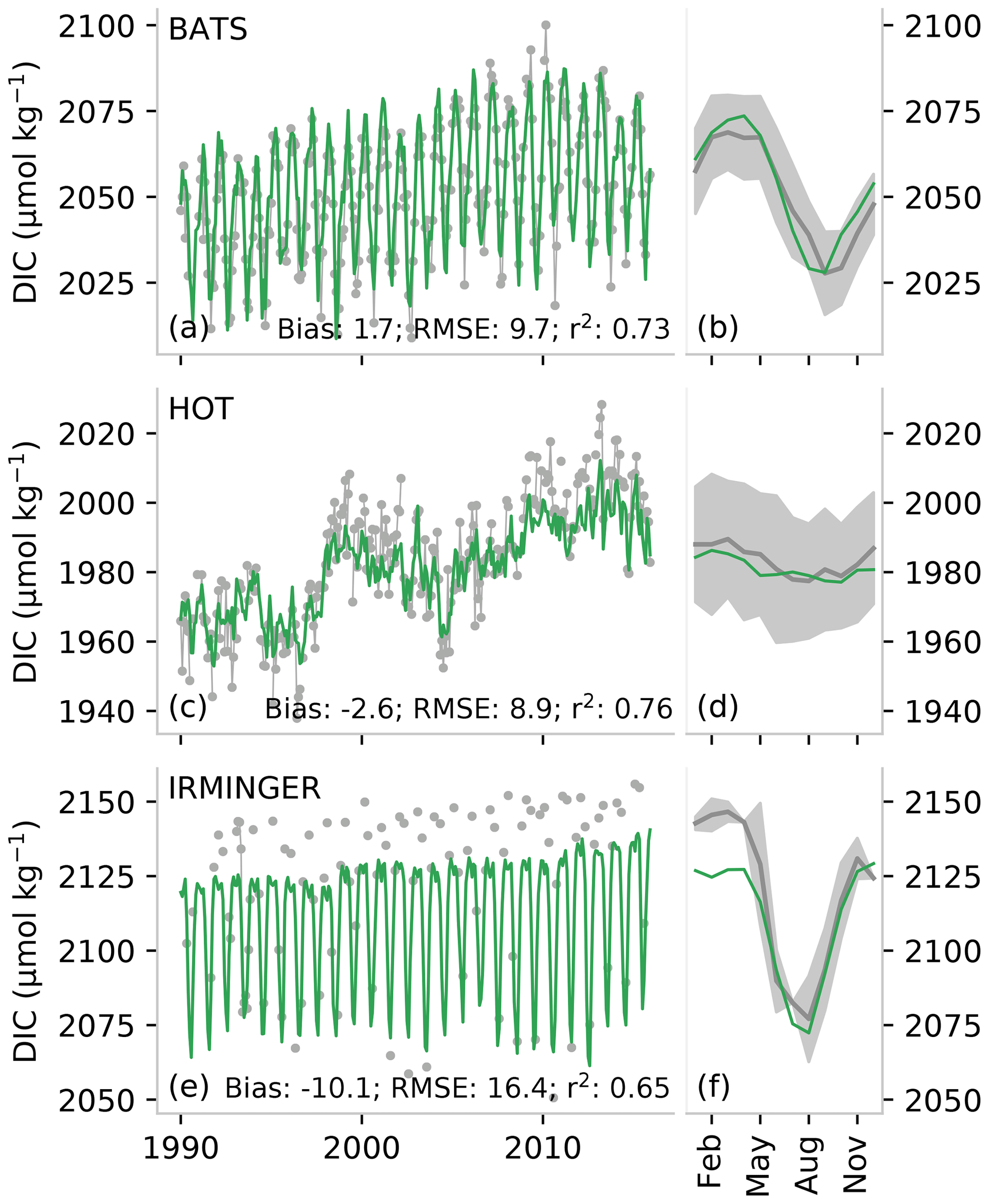
Figure 6 A comparison of observations from long-term observation stations (gray) with predicted dissolved inorganic carbon (DIC). The top row (a, b) shows data for the Bermuda Ocean Time-series Study (BATS), the middle row (c, d) shows data for the Hawaii Ocean Time-series (HOT), and the bottom row (e, f) shows data for the Irminger station. The narrow panels on the right show the average of the seasonal climatology for the time series, where the gray shading shows the standard deviation of the observations for the period 1990 to 2018, while the green line shows the average estimate.

3.2 Uncertainties of the calculated parameters

We determine the uncertainties of the calculated parameters in two ways. First, we propagate the uncertainties of pCO₂ and TA through pyCO2SYS (Orr et al., 2018; Humphreys et al., 2020) onto the computed parameters DIC, pH, and Ω. This yields an expected uncertainty that we refer to as a bottom-up total uncertainty estimate. Second, we obtain a top-down uncertainty estimate by comparing the calculated DIC and pH with independent measurements (see Table 4). We first describe the top-down estimates and then the bottom-up estimates. For the top-down estimate, we use the GLODAP DIC and pH data as our independent test of the method's performance. This is because these data are not used in any way in our estimation.

In the global mean, the computed DIC in OceanSODA-ETHZ has a very low bias compared with in situ GLODAP measurements (0.5 µmol kg⁻¹) (Table 4). Spatially, the DIC biases reveal a more nuanced picture, with large positive biases in the western equatorial Pacific and negative biases in the western equatorial Atlantic. The bias in the western equatorial Atlantic matches the negative bias in the pCO₂ in the same region; however, the source of the DIC bias in the Pacific is not clear from the pCO₂ and TA test data biases. The global mean of the top-down uncertainty estimate for DIC (16.3 µmol⁻¹ for the open ocean) is then perhaps a better reflection of the uncertainty as positive and negative values do not cancel each other out.

It is interesting to point out that the computed DIC in OceanSODA-ETHZ compares very favorably to directly estimated DIC products, such as that provided by NNGv2. Our uncertainty associated with the prediction error for DIC of 16.3 µmol⁻¹ is substantially better than theirs (23.1 µmol kg⁻¹) across all independent data.

The comparison of the DIC time series data (BATS, HOT, and Irminger stations) supports the findings of the global top-down estimates (Fig. 6). The biases are relatively low for HOT and BATS (−1.0 and 0.4 µmol kg⁻¹ respectively), but the bias is much larger at Irminger station (−6.9 µmol kg⁻¹), which is at a much higher latitude (64^∘ N) compared to HOT and BATS in the subtropics (<35^∘ N). However, this bias is not reflected in the zonal average of the seasonal biases (Fig. 5c). Similarly, the RMSE is also larger at Irminger station (14 µmol kg⁻¹) compared to HOT and BATS (∼ 9 µmol kg⁻¹) in the subtropics. Despite these differences in the top-down error, the same amount of variability is represented by the OceanSODA DIC for all three stations (∼ 0.76) owing to the larger seasonal cycle at Irminger station.

The pH comparison with the GLODAP pH measurements shows that OceanSODA-ETHZ has a negligible bias (0.001). As with DIC, regional biases in pH are larger than the global average, with the coastal and high-latitude oceans contributing significantly to the regional biases. The RMSE of pH with respect to GLODAP is also low (0.024) but is slightly outperformed by the RMSE of pH calculated with LIARv2 TA and FFNNv2 pCO₂ (made available in the FFNNv2 data set, 0.023). But given the uncertainty of GLODAP pH (0.01), the difference is negligible.

For the bottom-up estimate, we propagate the total uncertainty of pCO₂ and only the uncertainties associated with the measurement and prediction errors for TA. We do this to avoid including the representation error twice in the bottom-up estimate, as we hypothesize that the representation error of TA is largely accounted for by the representation error of pCO₂ and vice versa. We choose to use the representation error of pCO₂ rather than TA as the larger number of samples gives us greater confidence in the estimate. Moreover, we feel that the assumptions we make in the estimate of the TA representation error are larger than those for pCO₂, thus further justifying our choice in using only the representation error of pCO₂.

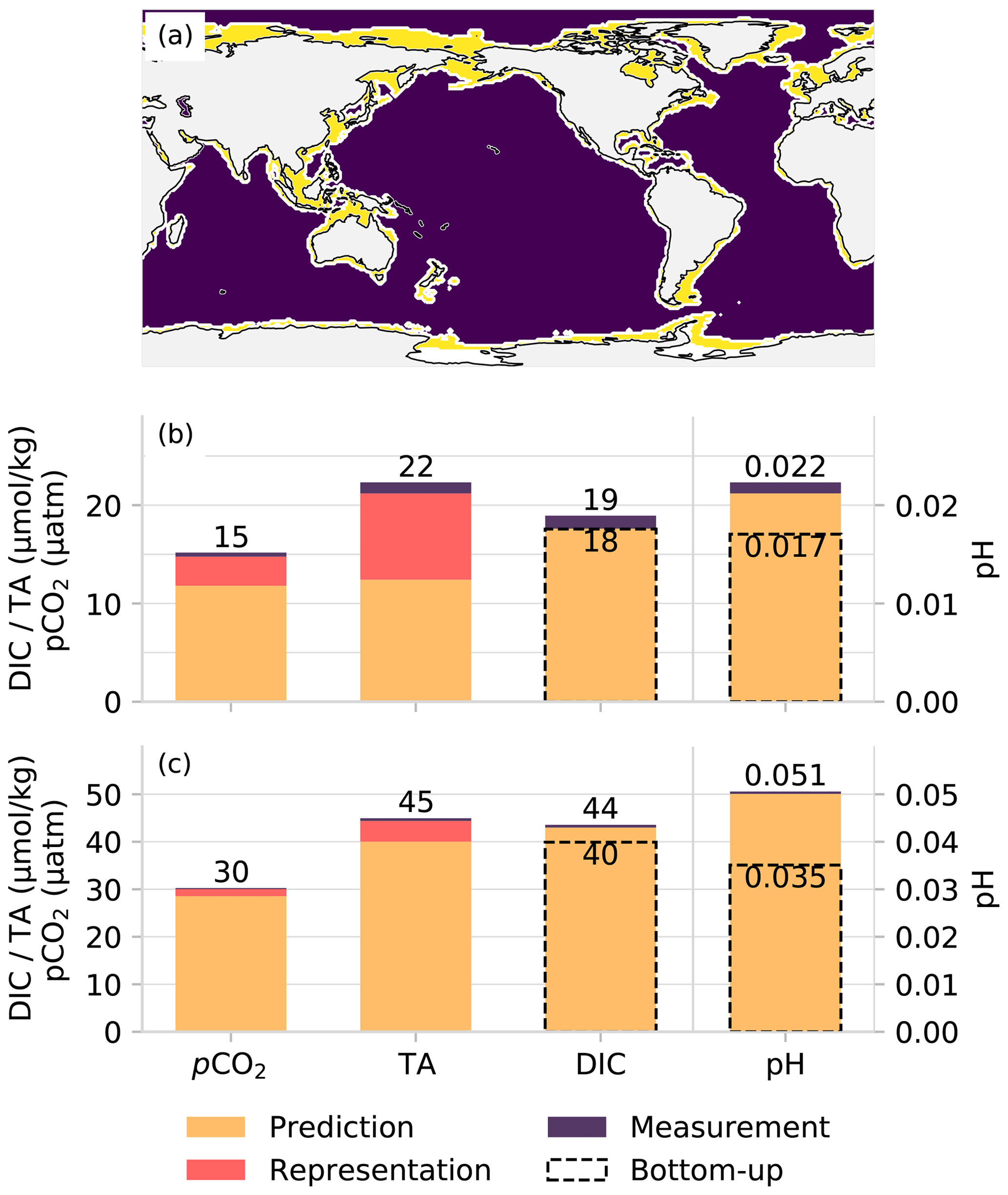
Figure 7 A comparison of propagated uncertainties with independent uncertainties as an assertion of the validity of uncertainty estimates. The map (a) shows the separation between coastal and open ocean, panel (b) shows the error contributions in the open ocean, and panel (c) shows those in the coastal ocean. The total uncertainty has been broken into the three different components. Note that the values represented by the bar plots are not equivalent to values in Table 3 as the latter shows pCO₂ and TA total uncertainties for test data only, while the bar charts show total uncertainties for all data; further, the breakdown of the error contributions is proportional to the contribution of the sum of the squares (see Eq. 2).

The comparison of top-down vs. bottom-up uncertainty estimates for open and coastal oceans is shown in Fig. 7, with values of the total uncertainties also shown. The top-down and bottom-up uncertainty estimates for DIC are relatively accurate, with the estimates being within 5 % of each other in the open ocean and 9 % in the coastal ocean. However, the estimates are not as coherent for pH where the bottom-up error is 23 % smaller than the top-down uncertainty in the open ocean. The difference is even bigger in the coastal ocean where the bottom-up uncertainty is 31 % smaller than the top-down uncertainty.

4 Results

4.1 Comparison with other climatologies

A spatial comparison between OceanSODA-ETHZ and existing products might reveal potential biases in our product if the bias is present in all comparisons. We compare TA against LIARv2 and NNGv2 (Carter et al., 2018; Broullón et al., 2018) by first taking the difference for each month and then calculating the average for these differences. The same approach is used to compare pCO₂ with SOMFFN and FFNNv2 (Landschützer et al., 2016; Denvil-Sommer et al., 2019).

The differences in TA between OceanSODA-ETHZ and NNGv2 and LIARv2 are on the same order of magnitude in the open ocean as the prediction error (13 µmol kg⁻¹) but are slightly larger on average for NNGv2 than for LIARv2 (Fig. 8a, b). There is also some agreement in the spatial pattern of the distribution, particularly in data-sparse parts of the Pacific Ocean and Indian Ocean. The larger differences may stem from the fact that both LIARv2 and NNGv2 are more constrained by spatial coordinates than GRaCER. NNGv2 uses latitude and longitude as predictors, while the LIARv2 approach interpolates the linear regression coefficients for every 5^∘ grid cell (Broullón et al., 2018; Carter et al., 2018). The divergence in data-sparse regions is thus not surprising. Although, it must be emphasized that this comparison serves more as a sanity check than as a ground-truthing exercise.

Figure 8 A comparison of the mean differences between TA (a, b) and pCO₂ (c, d) for OceanSODA-ETHZ and other published methods: (a) LIARv2, (b) NNGv2, (c) CMEMS-FFNNv2, and (d) MPI-SOMFFN. The markers in the North Pacific show the locations used in the comparison of the climatology in Fig. 11.

The differences between OceanSODA-ETHZ pCO₂ and FFNNv2 and SOMFFN are smaller and not as spatially coherent compared to those for TA. The differences are marginally larger for the OceanSODA-FFNNv2 than for OceanSODA-SOMFFN (Fig. 8c, d). This is consistent with the data in Table 4, where the metrics for the SOMFFN are very similar to OceanSODA-ETHZ. The smaller difference between the latter should not come as a surprise as the GRaCER approach is built on the two-step cluster-regression approach of the SOMFFN, while the FFNNv2 approach includes spatial coordinates (Landschützer et al., 2016; Denvil-Sommer et al., 2019). In general, the dissimilarity between the differences is encouraging as it indicates that OceanSODA-ETHZ is not consistently biased relative to SOMFFN and FFNNv2.

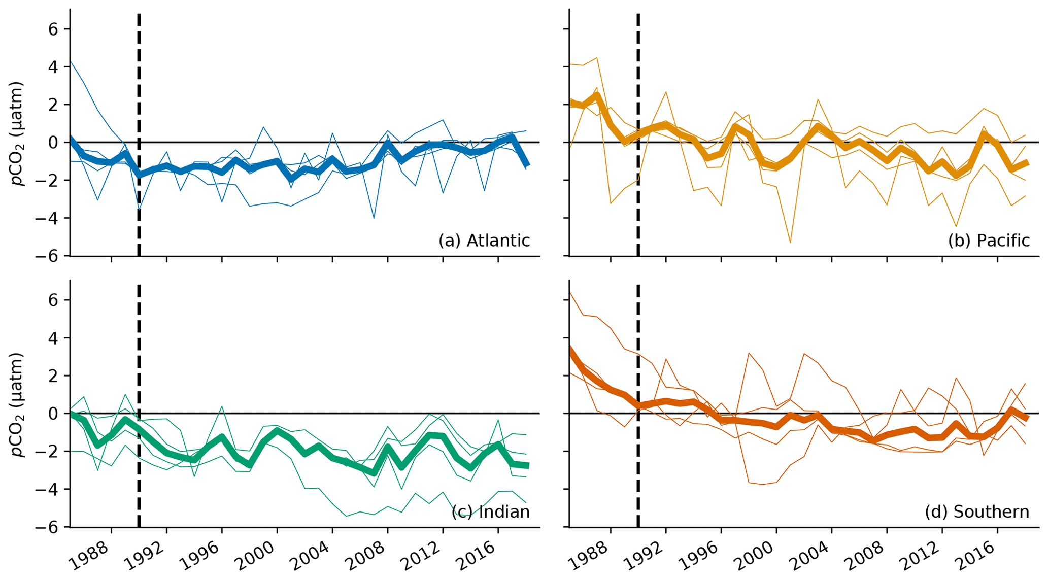
Figure 9 A basin–mean comparison of OceanSODA-ETHZ pCO₂ with four gap-filling methods: MPI-SOMFFN, JENA-MLS, CMEMS-FFNNv2, and CSIR-ML6. The thin lines show the differences compared to the individual methods, while the thick line shows the mean difference across the four methods. We do not show the Arctic Ocean as OceanSODA-ETHZ covers only 23 % of the region. The vertical dashed line in each figure marks the year 1990, where estimates prior to this period show biases in panels (b) and (c).

We also show the temporal evolution of the basin–mean differences between OceanSODA-ETHZ pCO₂ and other gap-filling methods (Fig. 9). In the Atlantic (Fig. 9a), OceanSODA-ETHZ pCO₂ is <2 µatm lower than the mean of the other gap-filling methods for the period 1990 to 2008. Thereafter, the difference is <1 µatm. In the Indian Ocean, our pCO₂ estimates have a persistent negative difference of ∼2 µatm (Fig. 9c). The comparison in the Pacific (Fig. 9b) is the most consistent with the other methods, with a slight positive difference in the beginning of the period (pre-1990). The OceanSODA-ETHZ estimates of pCO₂ in the Southern Ocean (Fig. 9d) have a large positive difference prior to 1990 – up to 6 µatm for one of the ensemble members. This difference quickly diminishes and is near zero by 1990. There is also a negative difference later in the period (2004 to 2015); however, the ensemble spread over this period is large.

The comparison with other methods illustrates that while gap-filling methods are converging on a global scale, there are regional differences. Further, large differences in pCO₂ between methods prior to 1990 indicate high uncertainty for this period.

4.2 Seasonal climatologies

The climatological mean spatial distribution of TA, pCO₂, DIC, pH, and Ω, obtained by averaging the estimates from 1985 through 2018 reveals a very rich and diverse pattern of variability with commonalities and differences (Fig. 10). The climatological maps are accompanied by Hovmöller diagrams that show the zonal average of the seasonal cycle for each of the variables (Fig. 11). We also show climatological time series for each of the variables at high-latitude (55^∘ N, 170^∘ W), midlatitude (30^∘ N, 170^∘ W), and low-latitude (10^∘ N, 170^∘ W) locations.

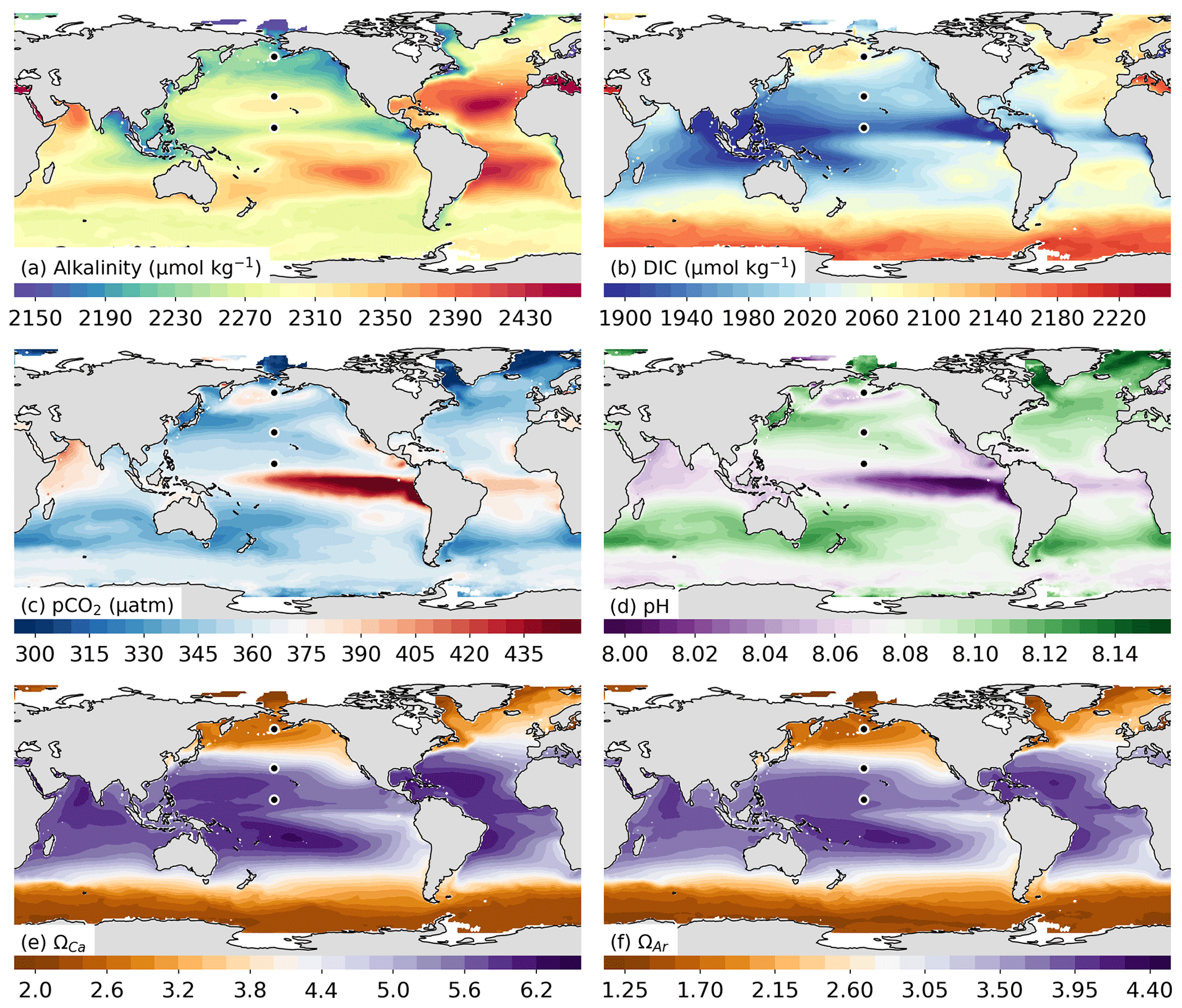
Figure 10 Mean maps of the GRaCER-based estimates for the period 1985–2018 for (a) total alkalinity and (c) pCO₂, as well as those of the computed variables, (b) dissolved inorganic carbon, (d) pH, (e) Ω_calc (saturation state with regard to calcite), and (f) Ω_arag (saturation state with regard to aragonite). The three black markers in each plot show the locations chosen for the seasonal analysis in Fig. 11f–j.

Total alkalinity shows the largest differences between basins, with the mean alkalinity being much higher in the saltier Atlantic than in the Pacific and Indian basins (Boutin et al., 2018) (Fig. 10a). The spatial variability of TA on a global scale exceeds the variability of the seasonal cycle (Fig. 11a, e). Seasonal variability of TA is on the order of 20 µmol kg⁻¹ at the chosen mid- and high-latitude locations, while the latitudinal gradient is as large as 150 µmol kg⁻¹. However, much of the TA seasonality is driven by seasonal changes in salinity due to precipitation and ice melt in the respective regions.

Dissolved inorganic carbon is more homogeneous across the basins but has a much larger meridional gradient than TA, amounting to more than 150 µmol kg⁻¹ (Fig. 10b). This meridional gradient is seasonally substantially more modified than is the case for TA, particularly in the high latitudes of the Northern Hemisphere where the seasonal cycle is as large as 100 µmol kg⁻¹ (Fig. 11b, g). The larger seasonal cycle in DIC is due to the carbon uptake by springtime phytoplankton blooms and stratification during the warmer seasons (Siegel et al., 2002). The magnitude of the springtime blooms is dampened by iron limitation in the Southern Ocean, visible by a smaller seasonal cycle amplitude (∼ 40 µmol kg⁻¹) (Watson et al., 2000; Tagliabue et al., 2017). However, the background DIC concentration in the Southern Ocean is much larger due to upwelling of DIC-rich circumpolar deep waters driven by the persistent westerlies south of 50^∘ S (Marshall and Speer, 2012).

The spatial distribution and seasonal cycles of pCO₂ and pH (Figs. 10c, d and 11c, d, h, i) are strongly negatively correlated due to the inverse stoichiometric relationship between dissolved aqueous CO₂ and [H⁺] (Dickson et al., 2007). The reduction in DIC is concomitant with the reduction in pCO₂ in the high latitudes due to the biological uptake of [CO₂] (Fig. 11g, h). However, this relationship does not hold true in the midlatitudes, where the slight decrease in DIC is contrasted by a relatively strong increase in pCO₂. This is due to the positive temperature dependence of pCO₂ (the opposite is true for pH) (Takahashi et al., 1993), which will be elaborated on in the discussion.

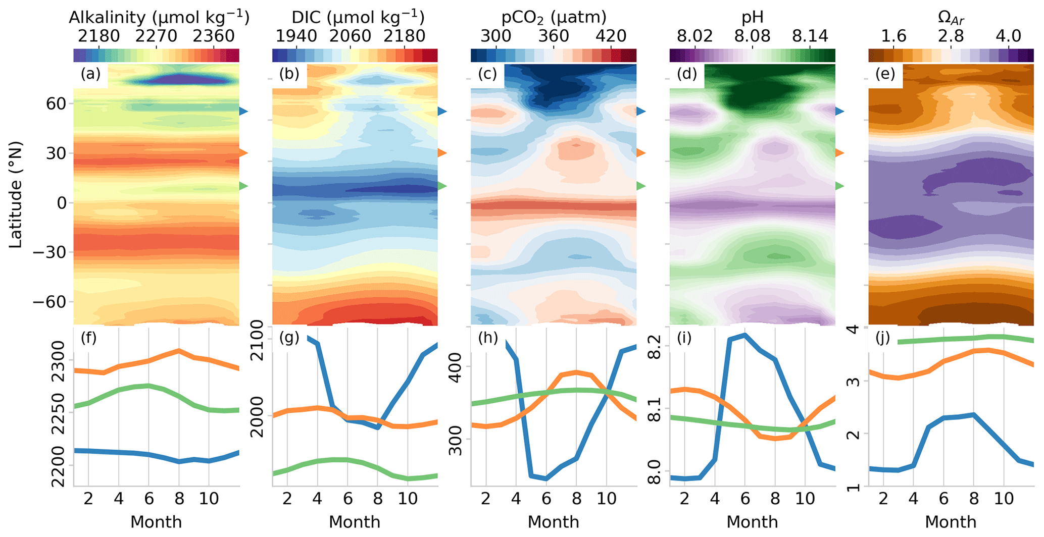
Figure 11 Hovmöller plots (a–e) showing the zonally averaged seasonal climatologies for (a) total alkalinity, (b) dissolved inorganic carbon, (c) pCO₂, (d) pH, and (e) aragonite saturation state (Ω_Ar). The second row of panels (f)–(j) shows the corresponding variables for a high-latitude (55^∘ N, 180^∘ E, blue), midlatitude (30^∘ N, 180^∘ E, orange), and low-latitude (10^∘ N, 180^∘ E, green) locations. The units for panels (f)–(j) correspond with the units in panels (a)–(e).

The spatial distribution of Ω (Figs. 10e, f and 11e, j) strongly reflects the concentration of the carbonate ion, which can be well approximated by the difference between TA and DIC (Sarmiento and Gruber, 2006). Given that the seasonal cycle of TA is much weaker than DIC, the latter dominates the seasonal cycle of Ω_Ar (Fig. 11e, j). This would also be true for Ω_Ca, which only differs from Ω_Ar in magnitude and not in distribution or seasonality (the latter is not shown).

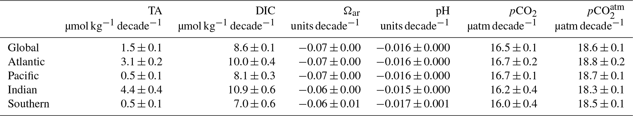
4.3 Global- and basin-scale long-term trends

The OceanSODA-ETHZ data set can provide important novel constraints on the long-term trends in ocean acidification. We determine the long-term trends by a linear regression approach, restricting the period to 1990 through 2018, thus leaving out the 1980s, where the estimates are much more uncertain.

The global- and basin-scale trends for pCO₂ are remarkably similar (varying by only about 0.5 µatm per decade around the global mean of 16.5 µatm per decade) (Table 5. The ocean trends are also very consistent with the trends in atmospheric CO₂ (∼ 18.6 µatm per decade), reflecting the fact that the CO₂ system in the surface ocean is following the increase in the atmosphere very closely globally as well as in all ocean basins. The atmospheric trend is slightly steeper than those in the ocean. This is as expected since the atmospheric CO₂ increase forces the ocean, leading to a slight delay, a reflection of an increase in the air–sea disequilibrium over time (see, e.g., discussion in Matsumoto and Gruber, 2005). This growth in the air–sea disequilibrium is the driving force behind the increase in the oceanic sink strength for anthropogenic CO₂ over time (Gruber et al., 1996).

The basin-scale consistency holds true for pH as well (−0.016 units per decade) and Ω_ar (−0.07 units per decade), where global values are very similar to those averaged across the different ocean basins. In contrast, there is more spatial variability in the DIC trends, but the overall magnitude of about 9 µmol kg⁻¹ per decade largely represents the uptake of anthropogenic CO₂ from the atmosphere. The spatial differences in the DIC trends are also mirrored in the spatial variations in the TA trends, with regions with higher DIC trends having higher TA trends. This makes sense in terms of positive trends in TA increasing the buffering capacity, hence permitting DIC to grow faster for the same increase in seawater pCO₂. The trends in TA themselves are driven almost entirely by salinity with a basin-scale correlation of 0.99 (see Cheng et al., 2020).

Table 5 Linear trends and their standard errors for OceanSODA-ETHZ variables for the period 1990 to 2018. All columns show increases per decade (decade⁻¹). All trends in the table are significant (P<0.05). We exclude the Arctic as the OceanSODA-ETHZ product only covers 23 % of this region and may thus give spurious trends. The ocean basins are defined by the map shown in Fig. A4.

5 Discussion

5.1 Choosing the appropriate machine learning configuration

Here we consider two notable decisions that have a large impact on the final estimates: (1) the use of the ensemble approach and (2) the choice of regression algorithm. For details on the minor choices, see Sect. A3 in the Appendix.

As previously motivated, we opt for the cluster-regression approach that is able to generalize estimates in sparse regions due to information sharing within a cluster. However, cluster boundaries are often semi-discrete, resulting in artifactual boundaries. This makes the output of cluster-regression approaches less suitable for studies where gradients over short time periods or distances are assessed, e.g., for the detection of extreme events. Our approach removes these boundaries and improves the robustness of the estimates by eliminating, to a large extent, the sensitivity of the regression to the clustering algorithm.

The second major consideration is the choice of regression algorithm. Our choice of different algorithms for TA and pCO₂ may seem peculiar. However, this decision was informed by the nature of the problems. While regressing TA and pCO₂ are conceptually similar, the size of each data set and the distribution of training samples set them apart. When gridded to a monthly by $\mathrm{1}{}^{\circ }\times \mathrm{1}{}^{\circ }$ resolution, the number of data are ∼300 000 for SOCAT pCO₂ and ∼16 000 for GLODAP TA – i.e., nearly 20 times more data for the former. However, the strong linear correlation between TA and salinity (r=0.96) compensates for the poor sampling distribution – that is, as long as the regression method is able to extrapolate – a criterion that the support vector regression (SVR) method meets.

pCO₂ is poorly correlated to any proxy, suggesting that the regression problem is more complex, thus requiring a method that is appropriately non-linear. Gradient boosted decision trees (GBDTs) and feed-forward neural networks (FFNNs) meet this criterion. But why not just use one of these approaches? Work by Gregor et al. (2019) found that an ensemble of methods (SVR, GBDTs, and FFNN) outperformed each individual member. And while SVR performed well in Gregor et al. (2019), the method does not scale to larger problems, which GBDTs and FFNNv2 are capable of, leading to our choice of the latter two. One critique of GBDTs in this application may be that, being a tree-based method, it is not able to extrapolate. However, we feel that the cluster-regression approach combined with the large number of training data for pCO₂ compensates for this shortcoming. GBDTs provide also provide useful diagnostics, such as feature importances, that, when combined with the GRaCER approach, provide useful information about the spatial and seasonal importance of the proxies.

5.2 Why are pH uncertainties less well constrained?

One of the novel contributions of this study is that we are able to assert the validity of our results by comparing the bottom-up (propagated) with the top-down uncertainties (in situ comparisons). Using this approach, we show that the uncertainty estimates of DIC are remarkably well constrained, with the top-down estimate being within 5 % of the bottom-up uncertainty estimate for the open ocean (Fig. 7b). The same statistics for pH yields a 23 % difference between the two budgets. The question is thus, why are pH bottom-up and top-down uncertainty estimates much less consistent?

To assess this problem from the bottom-up perspective, we need to consider the uncertainties of pCO₂ and TA. But given that the DIC uncertainty budgets are well constrained, we can, with some certainty, rule out the bottom-up uncertainty estimate as the source for the larger mismatch in pH.

The source of the mismatch must thus be driven primarily by uncertainties in the top-down perspective, where it may be that the representation error of pH is larger than for DIC. We rule out the measurement error as a contributor to the mismatch, as the bias of the measurements (provided accurate calibration to reference samples) should be normally distributed around zero. Thus, the representation error is the most likely candidate, due to the temperature- and pressure-sensitive nature of pH compared to the conservative nature of DIC with respect to the same variables (Dickson et al., 2007). This is important given that our surface pH data from GLODAP can be as deep as 30 m, while pCO₂ is typically measured at the intake depth of most ships, which is typically at 5 m (Bakker et al., 2016). A basic sensitivity study of the variability of pH in the surface layer shows that the median standard deviation of surface pH at a single station is 0.004 units (even when normalized to a standard temperature and depth). The same approach for DIC yields a standard deviation of 2 µmol kg⁻¹. This suggests that the vertical mismatch error of GLODAP alone already explains a good deal of the discrepancy in the uncertainty budgeting. One might reduce this uncertainty by placing tighter constraints on the definition of surface pH, limiting the depths between 3 and 15 m, for example, but at the loss of valuable test samples. The representation error (described in Sect. 3.1) could further explain the remaining disparity in the pH error budget.

5.3 Can we reduce the total uncertainty?

The last two decades have seen major improvements in the accuracy and precision of the TA and pCO₂ measurements, leading to substantial reductions in the measurement errors. The introduction of certified reference materials for TA and a standardized approach for measuring pCO₂ with reference gases means that the uncertainties associated with the measurements are low.

In contrast, the prediction uncertainty is the largest contributor to the total uncertainty for both DIC and TA, suggesting that this could be a fruitful avenue to pursue. However, current literature suggests that this is unlikely. Gregor et al. (2019) showed that, within a selection of six gap-filling methods, all achieved similar accuracy scores when compared with independent data, upon which the authors suggested that we have hit a wall.

This leaves the representation error, which contributes a moderate fraction to the total pCO₂ and TA uncertainties in the open ocean and even less in the coastal ocean. A back-of-the-envelope calculation shows that increasing the resolution of pCO₂ 4-fold (from monthly by 1^∘ × 1^∘ to 8-daily by 0.25^∘ × 0.25^∘) could decrease the representation error by 2.5 µatm (35 %) for the open ocean and 3.2 µatm for the coastal ocean (20 %). This is perhaps not as much as expected, but these small gains are larger than those that are currently being made with regard to the prediction errors (Gregor et al., 2019). This is not applicable for TA, where ungridded values are already used to train GRaCER and where the selection of the predictor variables is likely more important.

Why are these gains smaller than hoped? It may be that our gradient approach for calculating the representation error breaks down as the resolution increases due to the decreasing number of adjacent grid points. This is hardly surprising considering that 78 % of grid cells in the SOCAT v2019 monthly gridded product are represented by sampling on a single day that falls within that period (Bakker et al., 2016). Another possibility is that decreasing both the spatial and temporal resolution exposes the sharp mesoscale gradients that are otherwise averaged over at larger resolutions (Resplandy et al., 2009; Monteiro et al., 2015). With the currently available data, it seems as if the reduction to be made in the total uncertainty by increasing the resolution of the prediction data will be small.

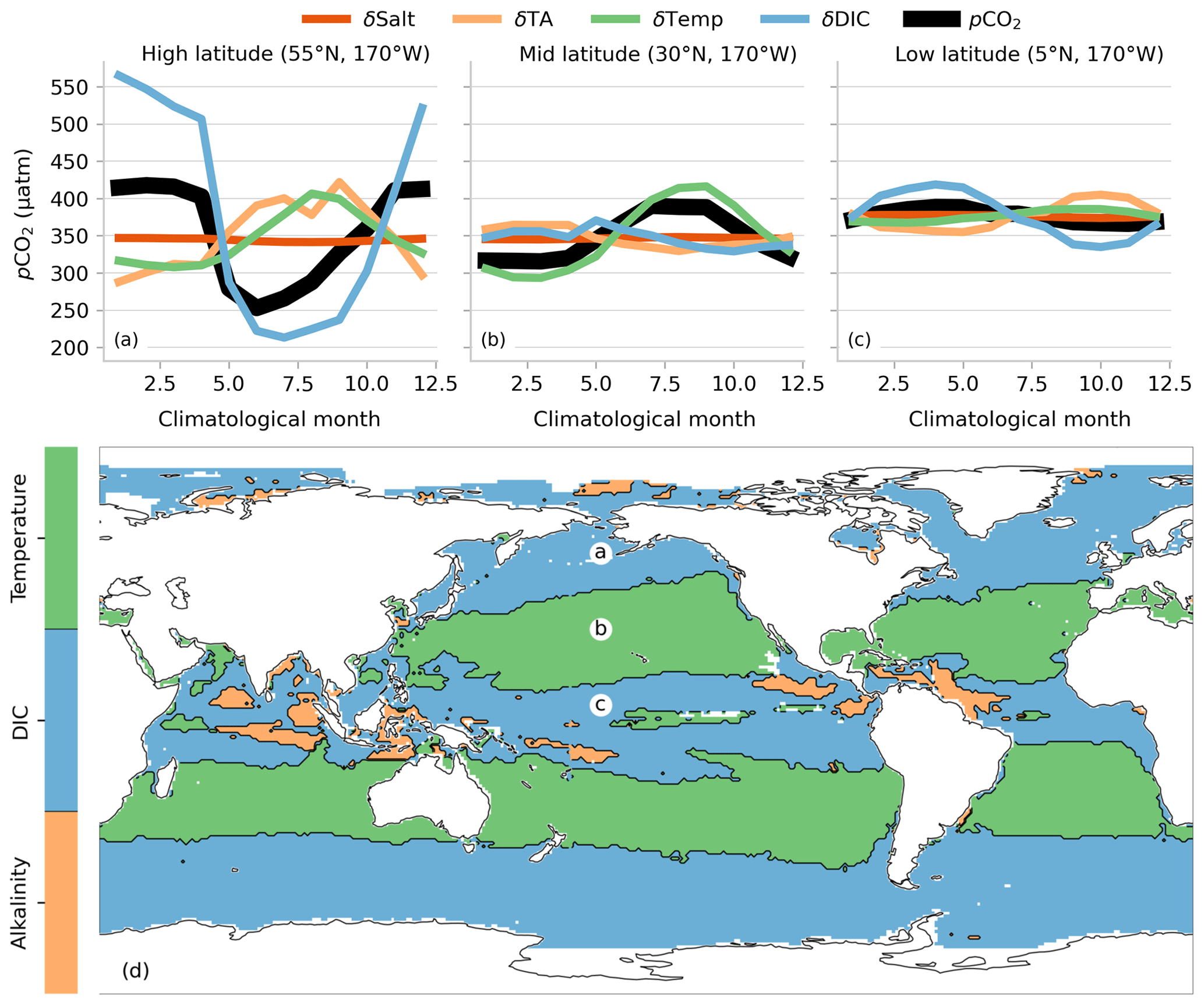
Figure 12 Attribution of DIC, TA, and temperature to the seasonal cycle of pCO₂. The top two figures show the seasonal cycle of pCO₂ and the drivers thereof for (a) high latitudes, (b) midlatitudes, and (c) low latitudes. These locations are shown with the markers in the Pacific Ocean in panel (c). The map (d) shows the dominant driver of the seasonal cycle for each region calculated as the value with the maximum seasonal amplitude.

5.4 Regional sensitivity of pCO₂ to driver variables

Here we demonstrate one of the possible ways in which the OceanSODA-ETHZ data can be used to gain further insight into the marine carbonate system.

We decompose and attribute the mean seasonal cycle variability of pCO₂ to its drivers, namely TA, DIC, temperature, and salinity. Past studies using observation based products have been limited to a simpler thermal/non-thermal decomposition of pCO₂ due to the lack of DIC and TA (Takahashi et al., 2002; Landschützer et al., 2015). This is thus the first time that a full decomposition of pCO₂ has been applied to observation-based data for a global domain. The decomposition is performed with pyCO2SYS by keeping all but one of the drivers constant (to the average) and assessing the influence on pCO₂ (Humphreys et al., 2020). This is similar to previous studies that applied an analogous decomposition to ocean simulation output (Lovenduski et al., 2007; Fassbender et al., 2018; Gallego et al., 2018). An important note to make, considering that we intend that OceanSODA-ETHZ is used for ocean acidification studies, is that the decomposition of pH would result in virtually the same contribution of the drivers (Dickson et al., 2007).

The seasonal amplitude of pCO₂ is driven predominantly by changes in DIC in the high and equatorial latitudes and by temperature in the midlatitudes (Fig. 12d). At first glance, these results may seem similar to those that the simpler thermal decomposition might result in, requiring only temperature. However, in regions where the seasonal amplitude of pCO₂ is smaller, the importance of TA becomes more apparent. For example, at the midlatitude station (Fig. 12b), TA and DIC synergistically act to dampen the impact of temperature on pCO₂. Conversely, at the equatorial station (Fig. 12c) the effect of TA on pCO₂ opposes that of the more dominant DIC. Further, there are regions in the tropics where TA is the dominant driver due to the weak seasonal cycle of both temperature and DIC.

5.5 Recommendations for use

In order to use the OceanSODA-ETHZ product in an optimal manner, it is important to be aware of its strengths and weaknesses.

The primary use of the OceanSODA-ETHZ data set is to determine and assess the seasonality, the interannual variations, and trends of ocean acidification thanks to its containing all relevant parameters of the marine carbonate system (Landschützer et al., 2015, 2016; Gregor et al., 2018; Keppler and Landschützer, 2019). However, users of the OceanSODA-ETHZ product should be aware of the fact that data prior to the 1990s should be treated with care due to the paucity of SOCAT pCO₂ training data during this period (Rödenbeck et al., 2015; Watson et al., 2020). This was recently demonstrated by Watson et al. (2020), who used an ensemble of various regression approaches to show that the spread of pCO₂ estimates prior to the 1990s is large due to the paucity of data. Similarly, Gregor et al. (2019) showed that pCO₂ estimates prior to 1990 tend to have a slightly positive bias.

The product is also very well suited for assessing models. Thanks to the spatially resolved estimates of uncertainty for TA and pCO₂ (Fig. A2), one cannot only assess the model–observation mismatches, but also weigh them with the appropriate uncertainties.

A strength of the OceanSODA-ETHZ product is that it extends further into the coastal margin than most previous studies (Iida et al., 2015; Landschützer et al., 2016; Denvil-Sommer et al., 2019). This is achieved (i) by including coastal observations during the training and (ii) by using a larger number of clusters compared to other clustering approaches (Landschützer et al., 2016; Watson et al., 2020). This permits us to better separate open-ocean and coastal variability through the inclusion of suitable variables in the clustering step (e.g., Chl a for pCO₂, and see Fig. A5 to see a representation of cluster boundaries). This gives us confidence in the coastal estimates of the climatological seasonal cycle. Our product is therefore comparable to that of Landschützer et al. (2020), who blended separate coastal and open-ocean pCO₂ products into a single climatological product with a monthly resolution (Landschützer et al., 2016; Laruelle et al., 2017).

The total uncertainties of our estimates in the coastal ocean are considerably larger compared to the open-ocean estimates (Fig. 7). This reflects the much higher spatiotemporal variability of the physical and chemical environment in the coastal ocean, leading to much higher variations in the marine carbonate system (Laruelle et al., 2017). Since our predictor variables are only partially reflecting this variability, a large portion of the high total uncertainty is due to a high representation error (Table 3). Increasing the resolution of the products may improve the total uncertainty of coastal estimates as done by Laruelle et al. (2017). Until we arrive at this point, the OceanSODA-ETHZ data should be used with care in the coastal ocean. Further, we recommend that researchers interested in the investigation of interannual variability and trends in the coastal ocean using the OceanSODA-ETHZ product should also look a the underlying in situ data to gain a better understanding of the variability, trends, and uncertainties for the coastal region of interest.

6 Code and data availability

Software for the GRaCER framework is available on Zenodo https://doi.org/10.5281/zenodo.4455354 (Gregor, 2021). The OceanSODA-ETHZ data set is available at https://doi.org/10.25921/m5wx-ja34 (Gregor and Gruber, 2020).

7 Summary

Our approach for estimating TA and pCO₂ is an evolution of the cluster-regression approach: we create an ensemble of estimates by repeating the cluster-regression step multiple times, each with a different variation of clustering. We call this approach the Geospatial Random Cluster Ensemble Regression (GRaCER). The result is an estimate that is more robust with better generalization, and the output does not have the discrete cluster boundaries that single-member cluster-regression approaches have.

We find that our estimates of TA are within the ballpark of previous methods with a prediction error (root mean square error) of 13 µmol kg⁻¹ for open-ocean estimates, while biases are <1 µmol kg⁻¹. Taking into consideration all sources of error (measurement and representation errors), the total uncertainty is 17 µmol kg⁻¹ for TA. The prediction error for pCO₂ in the open ocean is 12 µatm, also with a bias of <1 µatm. Including the measurement and representation errors for pCO₂ results in a total uncertainty of 14 µatm for the open ocean. We estimate the total uncertainty of DIC and pH to be 19 µmol kg⁻¹ and 0.022 units when compared with independent GLODAPv2 data for the open ocean. Finally, we compare the aforementioned top-down uncertainty estimates of DIC and pH with the bottom-up uncertainty estimates that are calculated by propagating the TA and pCO₂ total uncertainty estimates through the marine carbonate system. This budgeting approach shows that we have a good grasp on the uncertainties of DIC for both the open and coastal oceans. However, pH uncertainties are not as well resolved, most likely due to a mismatch in the representativity of the measured pH.

We demonstrate a use case of the OceanSODA-ETHZ data set in which we decompose the seasonal variability of pCO₂ into four driver components of DIC, TA, temperature, and salinity. We find that DIC is the dominant driver in the high and equatorial latitudes, while temperature contributes the majority of the signal in the subtropics. Importantly, DIC and temperature are antagonistic drivers of pCO₂, while alkalinity always acts in opposition to the stronger of the two primary drivers. We also show the strong constraints OceanSODA-ETHZ can pose on the long-term trends in ocean acidification.

Finally, OceanSODA-ETHZ will be maintained and updated for future work.

Appendix A: Supplement to the methods

A1 pCO₂ outlier removal

The first outlier removal method requires the pCO₂ to be adjusted from the ship intake temperature to the satellite SST as described by Goddijn‐Murphy et al. (2015):

$$\begin{array}{}\text{(A1)}& \begin{array}{rl}p{\mathrm{CO}}_{\mathrm{2}}^{\mathrm{SST}}& =p{\mathrm{CO}}_{\mathrm{2}}^{\mathrm{SOCAT}}\\ & \times \exp \left(\mathrm{0.0433}\cdot \left(T^{\mathrm{SST}}-T^{\mathrm{SOCAT}}\right)\right),\end{array}\end{array}$$

where the ship intake depth varies due to inconsistent depth between vessels and the water column state (e.g., well stratified or mixed). Here T^SST is the foundation temperature given by the Operational Sea Surface Temperature and Sea Ice Analysis (OSTIA) product (Good et al., 2020). The OSTIA product is matched to the ungridded $p{\mathrm{CO}}_{\mathrm{2}}^{\mathrm{SOCAT}}$ at daily by $\mathrm{0.25}{}^{\circ }\times \mathrm{0.25}{}^{\circ }$ resolution (Good et al., 2020). The corrected pCO₂ is then binned to monthly by $\mathrm{1}{}^{\circ }\times \mathrm{1}{}^{\circ }$ resolution without weighting. Data are excluded where the absolute difference between $p{\mathrm{CO}}_{\mathrm{2}}^{\mathrm{SST}}$ and $p{\mathrm{CO}}_{\mathrm{2}}^{\mathrm{SOCAT}}$ is larger than 40 µatm.

Secondly, we exclude data that lie outside the expected ranges for the monthly climatology of pCO₂. The expected ranges are defined using the interquartile range outlier detection method for each pixel in a given month with the following equation:

$$\begin{array}{}\text{(A2)}& {\displaystyle }\mathrm{IQR}=Q_{\mathrm{3}}-Q_{\mathrm{1}},\text{(A3)}& {\displaystyle }\text{lower limit}=Q_{\mathrm{1}}-\mathrm{IQR}\cdot \mathrm{1.5},\text{(A4)}& {\displaystyle }\text{upper limit}=Q_{\mathrm{3}}+\mathrm{IQR}\cdot \mathrm{1.5},\end{array}$$

where Q₁ and Q₃ are the 25th and 75th percentiles, respectively. This approach is only applied where there are enough data present for a particular month of the year.

A2 Target variable: ΔpCO₂ vs. pCO₂

In this study, one of the avenues that we explored was to predict ΔpCO₂ instead of pCO₂. The motivation for predicting ΔpCO₂ is that it might allow new measurements from recent years to add new information about the seasonal cycle in regions where sampling was previously seasonally biased, e.g., the SOCCOM float data (Gray et al., 2018). Bushinsky et al. (2019) showed that including the new information about the seasonal cycle of pCO₂ in machine learning estimates resulted in stronger winter outgassing, but their results could only show this for the period in which SOCCOM float data are present. One of the reasons that machine learning approaches are not able to propagate this information back through time is that the larger pCO₂ is anchored by the CO₂ concentrations that are used as a proxy. Atmospheric pCO₂ is required as a predictor variable to capture the interannual signal of pCO₂. Predicting ΔpCO₂ might thus allow one to remove atmospheric pCO₂ as a driver because the interannual term trend of pCO₂ is removed.

The results appeared promising, but on further investigation we found that the regressions that were trying to predict ΔpCO₂ were not able to represent the increasing strength of the sink. Furthermore, we found that the interannual variability of pCO₂ was reduced compared to results that include atmospheric xCO₂ as a driver. Ultimately, we abandoned the approach.

A3 Hyper-parameter selection for regression methods

A3.1 Total alkalinity: support vector regression

Hyper-parameters for the support vector regression (SVR) were chosen on a per-cluster basis using grid search cross validation, where unshuffled K-fold cross validation with five splits was used. The νSVR variety of the algorithm from the scikit-learn package in Python was used. The parameters C, γ, and ν were selected.

A3.2 pCO₂: gradient boosted decision trees

We used the LightGBM package to perform the gradient boosted regression with decision trees (GBDTs). The GBDT algorithm was trained using early stopping, which determines the number of trees used in the model – typically one of the most important hyper-parameters. Every fifth year from 1987 to 2019 was set aside as the validation data used in the early stopping. The total number of leaves per tree and the minimum number of training points per terminal leaf were both set to N^0.5, where N is the number of training points in a given cluster. The number of leaves per tree determines the size of the tree. The difference with LightGBM compared to other packages, like XGBoost, is that trees are grown on a leaf-wise basis rather than a level-wise basis, where the depth of the tree would be a more important hyper-parameter. The minimum number of training points per terminal leaf determines how many points are aggregated in an estimate – a small number could thus result in overfitting. The value N^0.5 was determined experimentally with a single ensemble member, where the optimal values were determined with K-fold cross validation. The results were in the ballpark of N^0.5, showing relatively low sensitivity to changes in these hyper-parameters. Further, the learning rate was set to 0.2, and L1 and L2 regularization were both set to 20.

A3.3 pCO₂: feed-forward neural network

Given that the problem of solving pCO₂ is not very complex (i.e., it is within the capability of a single layer neural network), the multi-layer perceptron regressor from the scikit-learn package was used. The size of the hidden layer for each cluster was determined by shuffled K-fold cross validation with five splits. The maximum number of weights in a hidden layer was set to N^0.55. Back propagation was performed using the Adam optimizer. The learning rate of the optimizer was selected in the cross-validation process. Early stopping was used to speed up the training process and prevent overfitting where one random third of the data were used in early stopping.

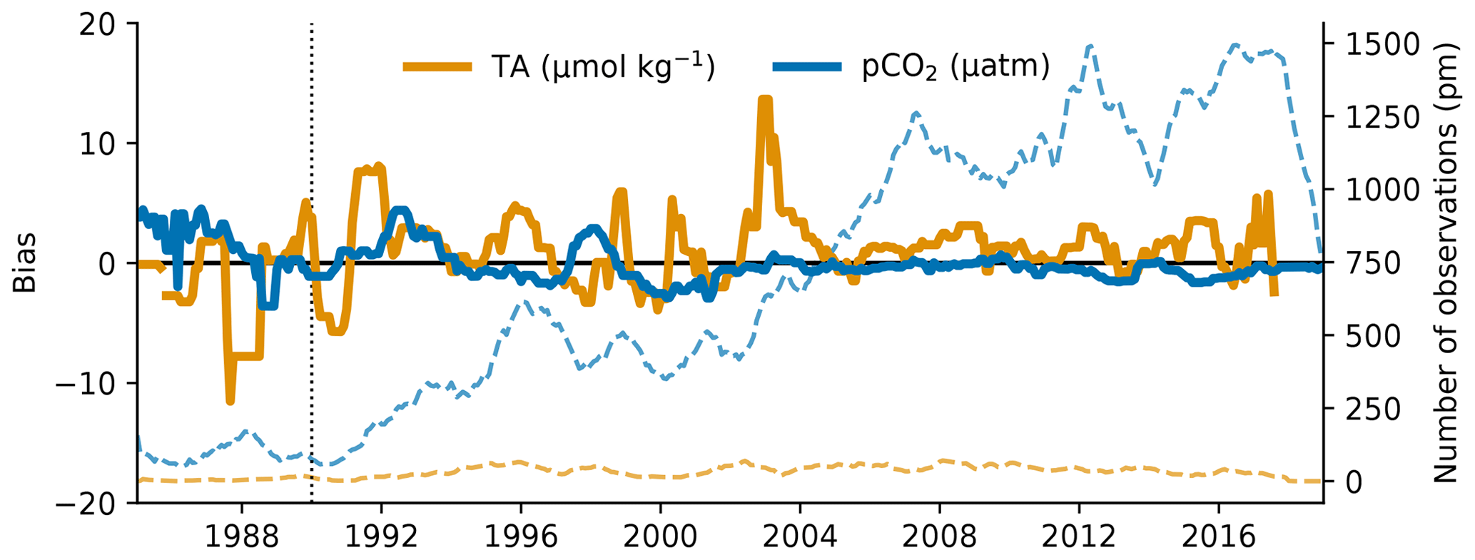
Figure A1 Time series of TA (orange) and pCO₂ (blue) estimates, with the respective training data sets (GLODAPv2 and SOCAT). The dashed lines show the number of training data (right axis). The vertical line shows the year 1990, before which OceanSODA-ETHZ pCO₂ estimates tend to be larger than other gap-filling estimates of pCO₂.

A4 GRaCER mapped cluster metrics

One of the advantages of using the GRaCER approach is that any metric can be mapped from the results to the appropriate clusters, resulting in an ensemble of metric scores. The possible metrics that can be applied include bias, root mean squared error, and mean absolute error. Further, these metrics can be applied to test data, meaning that the resulting scores can be based on test scores – that is, data that are unseen by the model during the training process, thus giving a true representation of the uncertainty. Given that the clusters used in this study are climatological, we can get fully mapped climatological estimates of uncertainty.

The uncertainty of TA remains fairly constant between summer and winter, with the Amazon plume showing increased uncertainty in the Northern Hemisphere summer (Fig. A2c).

The seasonal difference is larger for pCO₂ than for TA. For example, uncertainty in the Southern Ocean is much larger in the Southern Hemisphere summer (Fig. A2b, DJF) compared with winter (Fig. A2d, JJA).

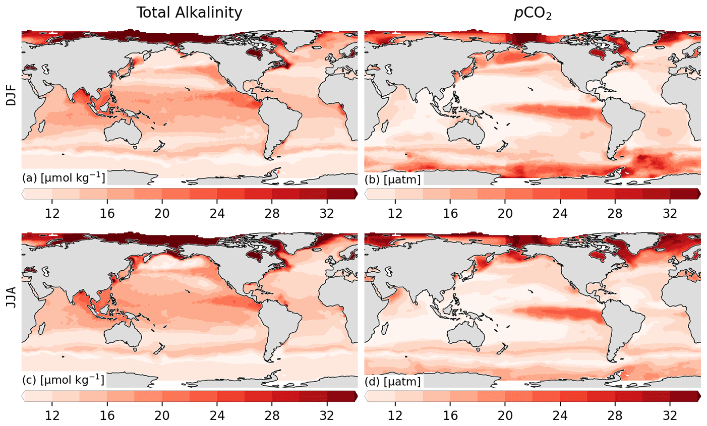
Figure A2 The Huber test scores mapped to the ensemble clusters for total alkalinity (TA) and pCO₂. The top row shows Huber scores averaged for December, January, and February (DJF) and the bottom row June, July, and August (JJA). The Huber score is a blend between root mean squared error (RMSE) and mean absolute error (MAE), where MAE is applied to values that are considered outliers. Only test data are used to calculate these climatological scores, meaning that the scores are based on GLODAP2 and SOCAT data for TA and pCO₂ respectively.

Similarly, the spatial distribution of feature importances can be determined with the GRaCER approach when using gradient boosted decision trees as the regression method (Fig. A3). Each ensemble member has a feature importance assigned to a cluster. When averaged over the ensemble members, a smoothed climatological estimate of feature importance can be estimated.

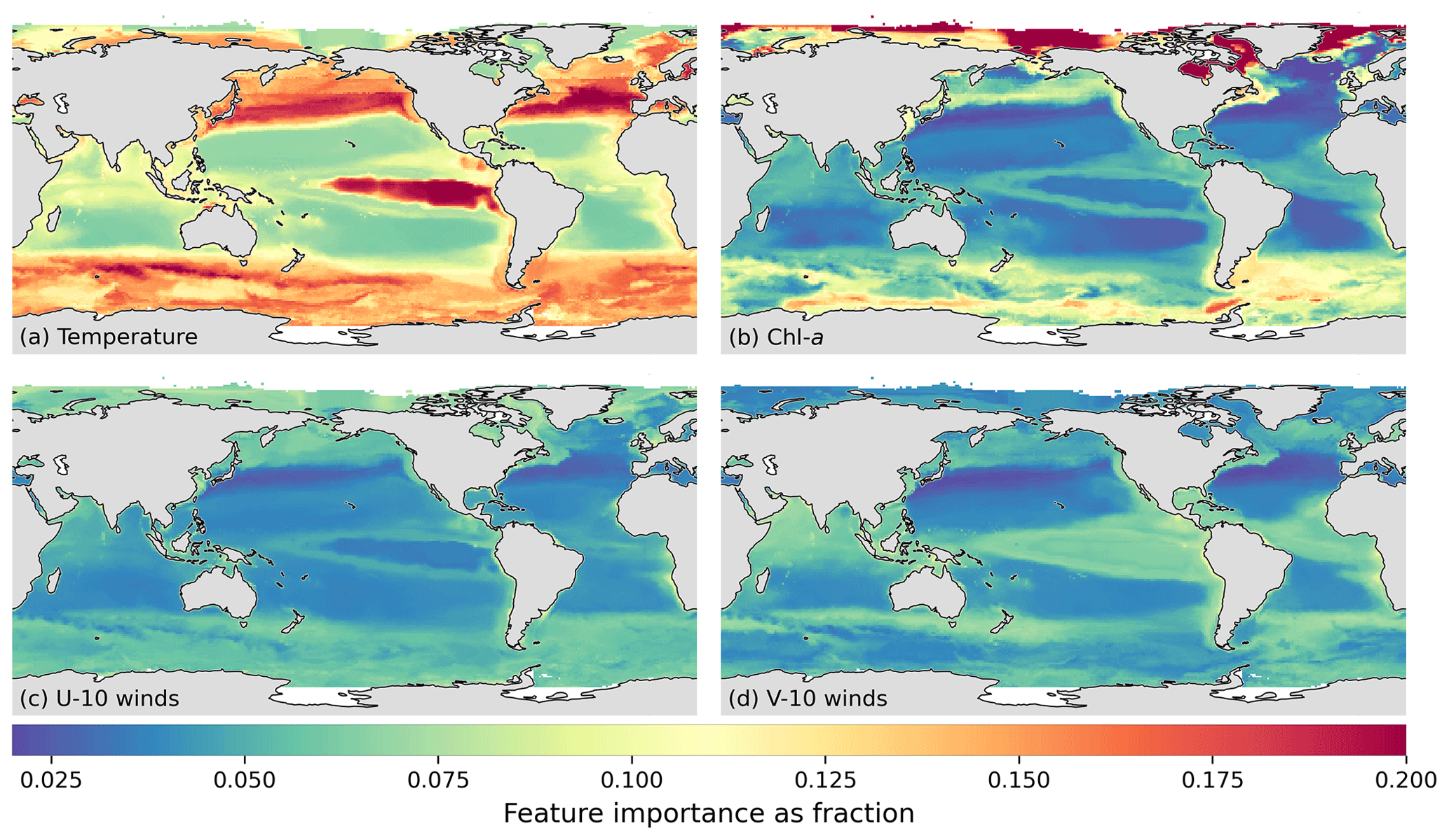
Figure A3 Feature importances determined by gradient boosted decision trees for pCO₂ predictions. A subset of four proxies are shown for the months of June, July, and August. The feature importances allow one to make informed decisions about the inclusion or exclusion of proxy variables. Here, temperature (a) is one of the more important features, Chl a is most important in the high northern latitudes, and the U and V components of the winds are important along the coastal regions, particularly the eastern boundary upwelling systems.

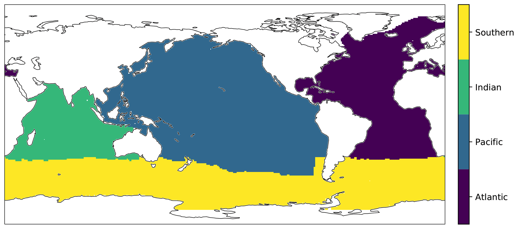
Figure A4 Ocean basin boundaries used in Table 5 as used by the RECCAP2 project (https://reccap2-ocean.github.io/regions/, last access: 21 November 2020). The Southern Ocean and North Atlantic boundaries are defined by biome boundaries defined in Fay and McKinley (2014).

A4.1 Cluster boundaries

The GRaCER method introduces the idea of using an ensemble of clusters, thus removing the variability that may be introduced in the clustering step. The location of the clusters varies from ensemble member to ensemble member. This creates a high-variance–low-bias scenario that is used by other ensemble methods such as random forests (Breiman, 2001). The location of these boundaries can give information about the mean distribution of the clusters. For example, locations where there are no cluster boundaries (≤1 in Fig. A5) indicate cluster centers that fall within the same cluster for the majority of time steps and ensemble members. While regions where cluster boundaries occur very often (>8 in Fig. A5) are indicative of regions where boundaries are found for most time steps and ensemble members.

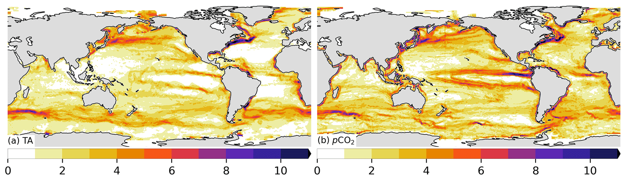
Figure A5 Map of the position of cluster boundaries across all ensemble members and months for (a) total alkalinity and (b) pCO₂. The white regions indicate locations that belong almost exclusively to the same cluster. Dark regions show where cluster boundaries are persistent.