Climatological distribution of dissolved inorganic nutrients in the western Mediterranean Sea (1981–2017)

The Western MEDiterranean Sea BioGeochemical Climatology (BGC-WMED, https://doi.org/10.1594/PANGAEA.930447) (Belgacem et al., 2021) presented here is a product derived from quality-controlled in situ observations. Annual mean gridded nutrient fields for the period 1981–2017 and its sub-periods 1981–2004 and 2005–2017 on a horizontal $\mathrm{1}/\mathrm{4}$^∘ × $\mathrm{1}/\mathrm{4}$^∘ grid have been produced. The biogeochemical climatology is built on 19 depth levels and for the dissolved inorganic nutrients nitrate, phosphate and orthosilicate. To generate smooth and homogeneous interpolated fields, the method of the variational inverse model (VIM) was applied. A sensitivity analysis was carried out to assess the comparability of the data product with the observational data. The BGC-WMED was then compared to other available data products, i.e., the MedBFM biogeochemical reanalysis of the Mediterranean Sea and the World Ocean Atlas 2018 (WOA18) (its biogeochemical part). The new product reproduces common features with more detailed patterns and agrees with previous records. This suggests a good reference for the region and for the scientific community for the understanding of inorganic nutrient variability in the western Mediterranean Sea, in space and in time, but our new climatology can also be used to validate numerical simulations, making it a reference data product.

1 Introduction

Ocean life relies on the loads of marine macro-nutrients (nitrate, phosphate and orthosilicate) and other micro-nutrients within the euphotic layer. They fuel phytoplankton growth, thus maintaining the equilibrium of the food web. These nutrients may reach deeper levels through vertical mixing and remineralization of sinking organic matter. Ocean circulation and physical processes continually drive the large-scale distribution of chemicals (Williams and Follows, 2003) toward a homogeneous distribution. Therefore, nutrient dynamics is important to understand the overall ecosystem productivity and carbon cycles. In general, the surface layer is depleted in nutrients in low-latitude regions (Sarmiento and Toggweiler, 1984), but in some ocean regions, called high-nutrient–low-chlorophyll (HNLC) regions, nutrient concentrations tend to be anomalously high, particularly in areas of the North Atlantic and Southern Ocean, as well as in the eastern equatorial Pacific and in the North Pacific; see, e.g., Pondaven et al. (1999). In the Mediterranean, the surface layer is usually nutrient-depleted. Most studies show that nitrate is the most common limiting factor for primary production in the global ocean (Moore et al., 2013), while others show evidence that phosphate may be a limiting factor in some specific areas, as is the case of the Mediterranean Sea (Diaz et al., 2001; Krom et al., 2004).

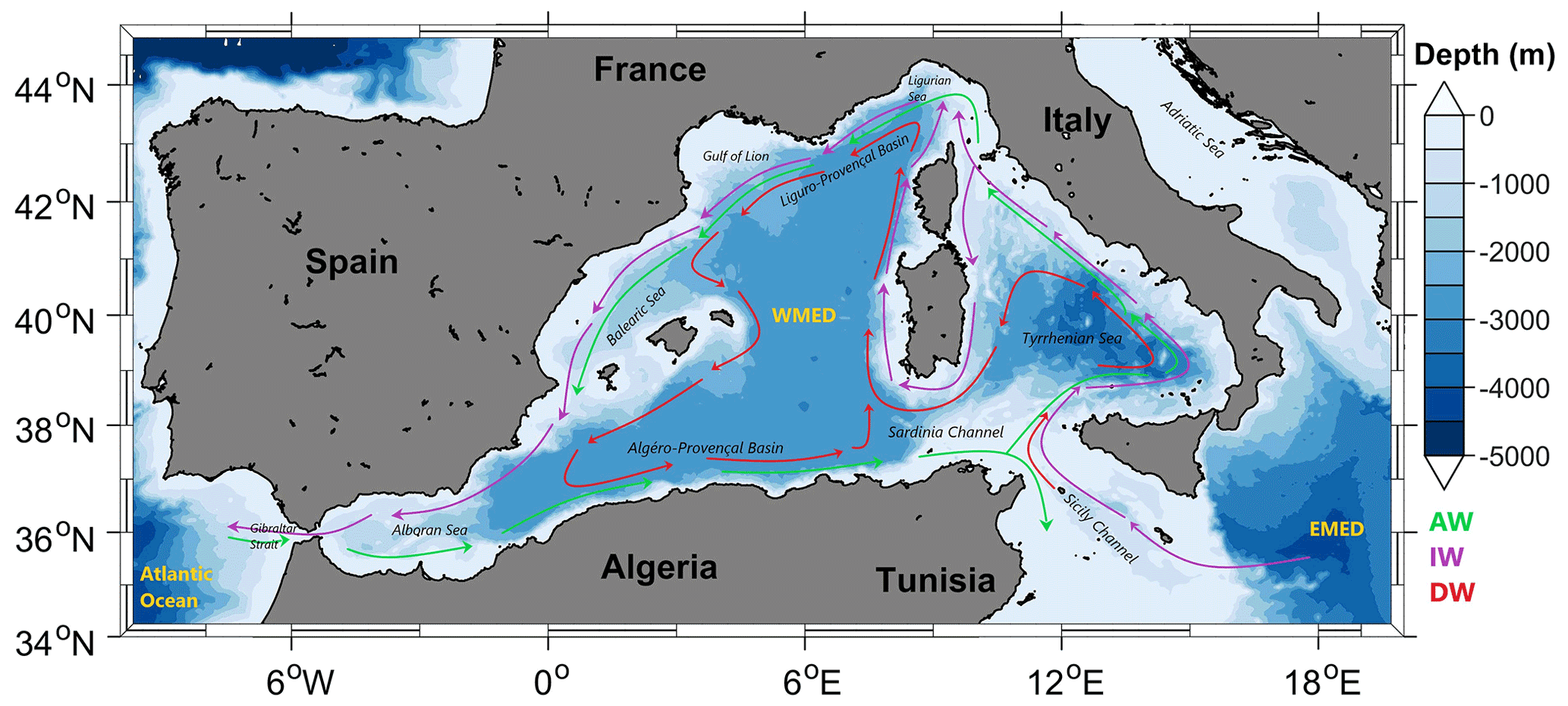
Figure 1 Map of the western Mediterranean Sea showing the main regions with a sketch of the AW, IW and DW major paths.

Being an enclosed marginal sea, the Mediterranean Sea exhibits an anti-estuarine circulation, responsible for its oligotrophic character (Bethoux et al., 1992; Krom et al., 2010) and acting like a subtropical anticyclonic gyre. The Atlantic water (AW), characterized by low-salinity and low-nutrient content, enters the western Mediterranean Sea (WMED) at the surface, through the Strait of Gibraltar, and moves toward the eastern Mediterranean Sea (EMED), crossing the Sicily Channel (Fig. 1). In the Levantine Sea and in the Cretan Sea, the AW becomes saltier, warmer and denser, and it sinks to intermediate levels (200–500 m) to form the intermediate water (IW; Schroeder et al., 2017). The IW (which may also be called Levantine Intermediate Water or Cretan Intermediate Water, LIW or CIW) flows westward across the entire Mediterranean Sea to the Atlantic Ocean (Fig. 1). As for the deep layer, the Western Mediterranean Deep Water (WMDW) is formed in the Gulf of Lion through deep convection (Testor et al., 2018; MEDOC Group, 1970; Durrieu de Madron et al., 2013), while the Eastern Mediterranean Deep Water (EMDW) is formed in the Adriatic Sea and occasionally in the Aegean Sea (Lascaratos et al., 1999; Roether et al., 1996, 2007).

The Mediterranean Sea is known to be a hotspot for climate change (Giorgi, 2006; Cheng et al., 2021). During the early 1990s, the deep water (DW) formation area of the EMED shifted from the Adriatic Sea to the Aegean Sea. This event is known as the Eastern Mediterranean Transient (EMT; Roether et al., 1996, 2007, 2014; Roether and Schlitzer, 1991; Theocharis et al., 2002). As a consequence, the intermediate and deep waters of the EMED became saltier and warmer (Lascaratos et al., 1999; Malanotte-Rizzoli et al., 1999). The EMT affected the WMED as well, not only changing the thermohaline characteristics of the IW and concurring with the preconditioning of the Western Mediterranean Transition (WMT; Schroeder et al., 2016), which set the beginning of a rapid warming and salting of the deep layers in the WMED from 2005 (Schroeder et al., 2006, 2010, 2016; Piñeiro et al., 2019). Over the last decade, it has been evidenced that heat and salt content have been increasing all over the deep western basin (Schroeder et al., 2016).

Changes in circulation due to an increased stratification limit the exchange of materials between the nutrient-rich deep layers and the surface layers. Understanding the peculiar oligotrophy of the Mediterranean Sea is still a challenge since there is no exact quantification of nutrient sinks and sources. Studies like those of Crispi et al. (2001), Ribera d'Alcalà et al. (2003), Krom et al. (2010) and Lazzari et al. (2012) related the horizontal spatial patterns in nutrient concentrations mainly to the anti-estuarine circulation which exports nutrients to the Atlantic Ocean, showing a decreasing tendency of nutrient concentrations toward the east, as opposed to the salinity horizontal gradient. Others related it to the influence of the atmospheric deposition (Bartoli et al., 2005; Béthoux et al., 2002; Huertas et al., 2012; Krom et al., 2010) and river discharges that are rich in nitrate and deficient in phosphate (Ludwig et al., 2009), which might explain the peculiarity in both the EMED and the WMED.

Lazzari et al. (2016) also argued that the variations in phosphate are regulated by atmospheric and river inputs like those of the Ebro and Rhône (Ludwig et al., 2009).

These variations, together with anthropogenic perturbations, affect the spatial distribution of nutrients (Moon et al., 2016), and temporal variability is still unresolved.

De Fommervault et al. (2015) reported a decreasing phosphate and an increasing nitrate concentrations trend between 1990 and 2010, based on a time series (DYFAMED) in the Ligurian Sea, while Moon et al. (2016) evidenced an increase between 1990 and 2005 and a gradual decline after 2005 in both nitrate and phosphate in the WMED and EMED.

At the global scale, most of the biogeochemical descriptions are based on model simulations and satellite observations (using sea surface chlorophyll concentrations; Salgado-Hernanz et al., 2019) but also on the increasing use of Biogeochemical Argo floats (D'Ortenzio et al., 2020; Lavigne, 2015; Testor et al., 2018), since in situ observations of nutrients are generally infrequent and scattered in space and time. For this reason, climatological mapping is often applied to sparse in situ data in order to understand the biogeochemical state of the ocean representing monthly, seasonally or annually averaged fields.

Levitus (1982) was the first to generate objectively analyzed fields of potential temperature, salinity and dissolved oxygen and to produce a climatological atlas of the world ocean.

Later on, the World Ocean Atlas (WOA), the North Sea climatologies and the global ocean carbon climatology resulting from the GLODAP data product (Key et al., 2004; Olsen et al., 2020; Lauvset et al., 2021) used the Cressman analysis (1956) with a modified Barnes scheme (Barnes, 1964, 1994). In 1994, the first World Ocean Atlas (WOA94; Conkright et al., 1994) was released, integrating temperature, salinity, oxygen, phosphate, nitrate and silicate observations. Every 4 years there is a new release of the WOA with an updated World Ocean Database (WOD).

Table 1 Overview of the existing inorganic nutrient climatologies in the western Mediterranean Sea.

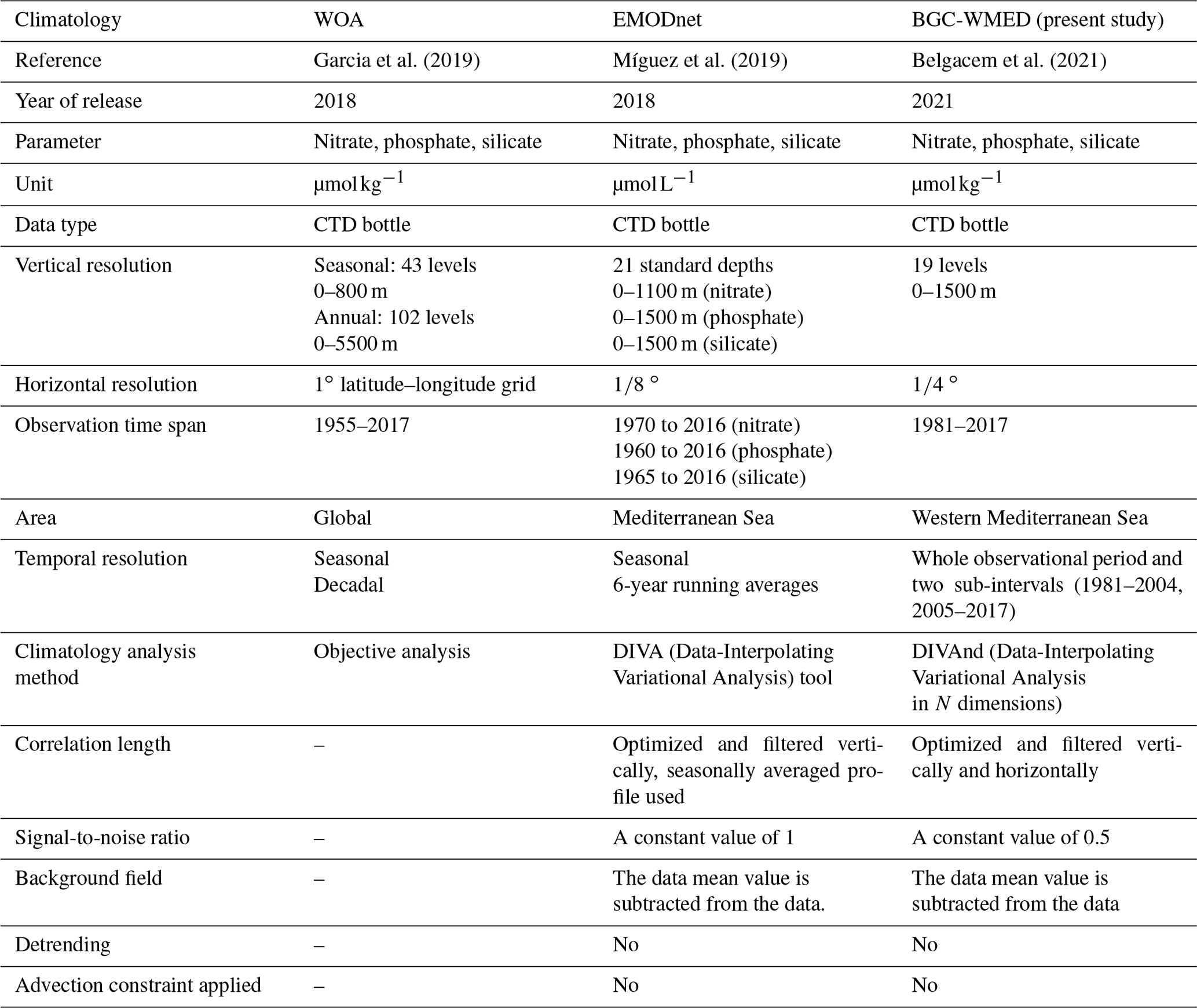
On the regional scale, the first salinity and temperature climatology of the Mediterranean Sea was produced by Hecht et al. (1988) for the Levantine Basin. Picco (1990) was also among the first to describe the WMED between 1909 and 1987. In 2002, the MEDAR/MEDATLAS group (Fichaut et al., 2003) archived a large number of biogeochemical and hydrographic in situ observations for the entire region and used the variational inverse model (VIM; Brasseur, 1991) to build seasonal and interannual gridded fields. In 2006, the EU SeaDataNet project integrated all existing data to provide temperature and salinity regional climatology products for the Mediterranean Sea using the VIM as well (Simoncelli et al., 2016), and dissolved inorganic nutrient (nitrate, phosphate and silicate) 6-year centered averages from 1965 to 2017 are available on the EMODnet (the European Marine Observation and Data Network) chemistry portal (https://www.emodnet-chemistry.eu/, last access: 3 January 2020​​​​​​​​​​​​​​). Within this context, in this study, regional climatological fields of in situ nitrate, phosphate and silicate, using the Data-Interpolating Variational Analysis in N dimensions (DIVAnd; Barth et al., 2014), are presented here, providing a high-resolution field contributing to the existing products (Table 1).

The aims of this study are to give a synthetic view of the biogeochemical state of the WMED, to evaluate the mean state of inorganic nutrients over 36 years of in situ observations and to investigate the effect of the WMT on the biogeochemical properties.

The paper is organized as follows: Sect. 2 describes the data sources used and the quality check; Sect. 3 is devoted to the methodology; Sect. 4 presents the main results including a comparison of the new climatology with other products. At the end, we address the change in biogeochemical characteristics before and after the WMT.

2 Data

The climatological analysis depends on the temporal and spatial distribution of the available in situ data and the reliability of these observations. Due to the scarcity of biogeochemical observations in the WMED, merging and compiling data from different sources was necessary.

Table 2 Number of inorganic nutrient profiles and data sources.

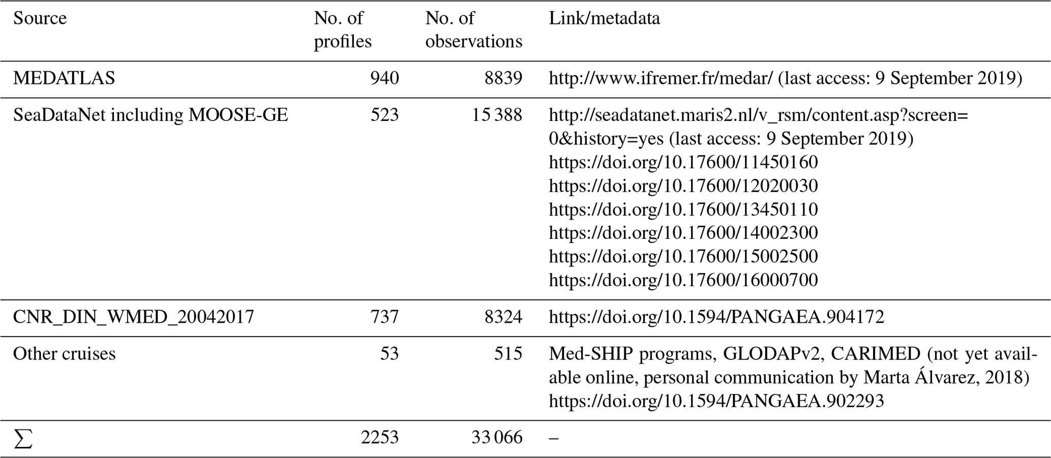
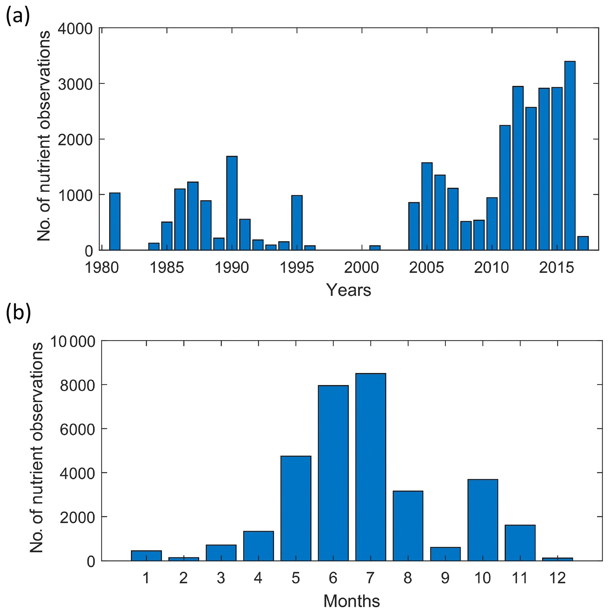
Figure 2 Temporal distribution of nutrient observations used for producing the BGC-WMED fields (1981–2017), (a) yearly distribution and (b) monthly distribution.  

Figure 3 (a) Nutrient data density used for climatology analysis. Observations are binned in a regular $\mathrm{1}/\mathrm{2}$^∘ × $\mathrm{1}/\mathrm{2}$^∘ latitude–longitude grid for each year over the period 1981–2017. Locations of the stations included in the analysis are shown as black dots. (b) Data distribution per depth range (i.e., at 800 m, observations between 800–1000 m are included).

2.1 Data sources

In total, 2253 in situ inorganic nutrient profiles are the base of the biogeochemical climatology of the WMED (Table 2) that is described here. These profiles cover the period 1981–2017 and come from the major data providers existing in the Mediterranean Sea, i.e.,  the MEDAR/MEDATLAS (1981–1996; Fichaut et al., 2003), the recently published CNR_DIN_WMED_20042017 biogeochemical dataset (2004–2017) (Belgacem et al., 2020), the MOOSE-GE cruises (Mediterranean Ocean Observing System for the Environment – Grande Échelle program) (2011–2016; Testor et al., 2011, 2012, 2013, 2014, 2015; Coppola, 2016) stored in the SeaDataNet data product (2001–2016) and EMODnet, GLODAPv2 (https://www.glodap.info/, last access: 2 November 2020​​​​​​​​​​​​​​) and CARIMED (http://hdl.handle.net/10508/11313, last access: 1 November 2020​​​​​​​​​​​​​​​​​​​​​) data products, and other data collected during Med-SHIP programs (Schroeder et al., 2015). All datasets are from a selection of oceanographic cruises carried out within the framework of European projects such as the HYdrological cycle in the Mediterranean EXperiment (HyMeX) Special Observation Period 2 (Estournel et al., 2016) and the DEnse Water EXperiment (DEWEX; CNRS-INSU, https://mistrals.sedoo.fr/MERMeX/, last access: 3 September 2021) project or by regional institutions having as objectives the investigation of the deep water convection and the biogeochemical properties of the WMED. Data were chosen to ensure high spatial coverage (Fig. 3).

2.2 Data distribution

The data distribution per year is shown in Fig. 2a. Most observations were collected between 1981 and 1995 and between 2004 and 2017, with a marked gap between 1997 and 2003. The measurement distribution differs from month to month (Fig. 2b) and tends to be biased toward the warm season. Very few measurements were made during December–January–February, and June and July are the months with the highest number of available observations (> 7000). Consequently, the climatological product may be considered more representative of spring and summer conditions.

Figure 3a shows the regional distribution of nutrient measurements, while Fig. 3b indicates the number of observations found in each depth range around the standard levels chosen for the vertical resolution of the climatology.

Hydrological and biogeochemical measurements have always been repeatedly collected along several repeated transects, known as key regions, such as the Sicily Channel and the Algéro-Provençal subbasin; likewise, the northern WMED is a well-sampled area as it is an area of DW formation. Observation density is still scarce (fewer than 100 observations) in some areas like the northern Tyrrhenian Sea.

The total number of measurements at each depth range underlines similar remarks: an uneven distribution that needs to be considered in the selection of the vertical resolution to estimate the climatological fields. However, the use of 36 years of nutrient measurements to generate the climatological fields significantly reduces the error field. In our case we take into account the irregular distribution in seasons and different years. A climatological gridded field was computed by analyzing observations of three time periods regardless of the month: 1981–2017 and the subsets 1981–2004 and 2005–2017. We chose these subsets to investigate the effect of the WMT on nutrient distribution.

2.3 Data quality check

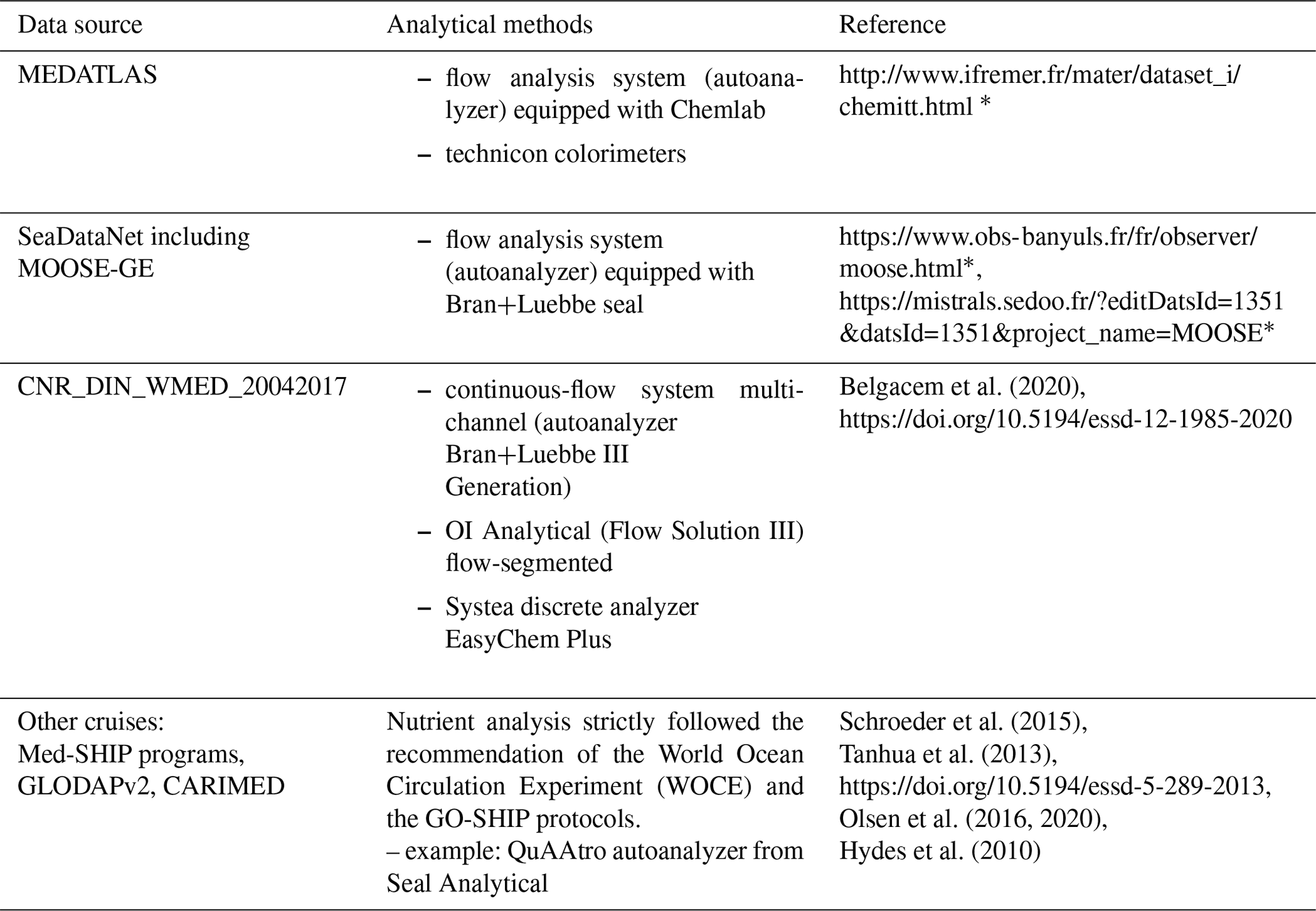
Data were gathered from different data sources and different analytical methods (Table A1.); thus before merging them, observations were first checked for duplicates (the number of profiles listed in Table 2 refers to all data after removing duplicate measurements). The criterion to detect and remove duplicates is simple: observations collected during the same cruises extracted from the different sources were removed. Since profiles were measured during specific cruises (identified with a unique identification code) at specific times, data from duplicate cruises were removed.

Then, data were converted to a common format (similar to the .csv CNR_DIN_WMED_20042017 data product; Belgacem et al., 2019). This recently released product contains measurements covering the WMED from 2004 to 2017. The data of the CNR_DIN_WMED_20042017 product have undergone a rigorous quality control process that was focused on a primary quality check of the precision of the data and a secondary quality control targeting the accuracy of the data; details about the adjustments and the applied corrections can be found in Belgacem et al. (2020).

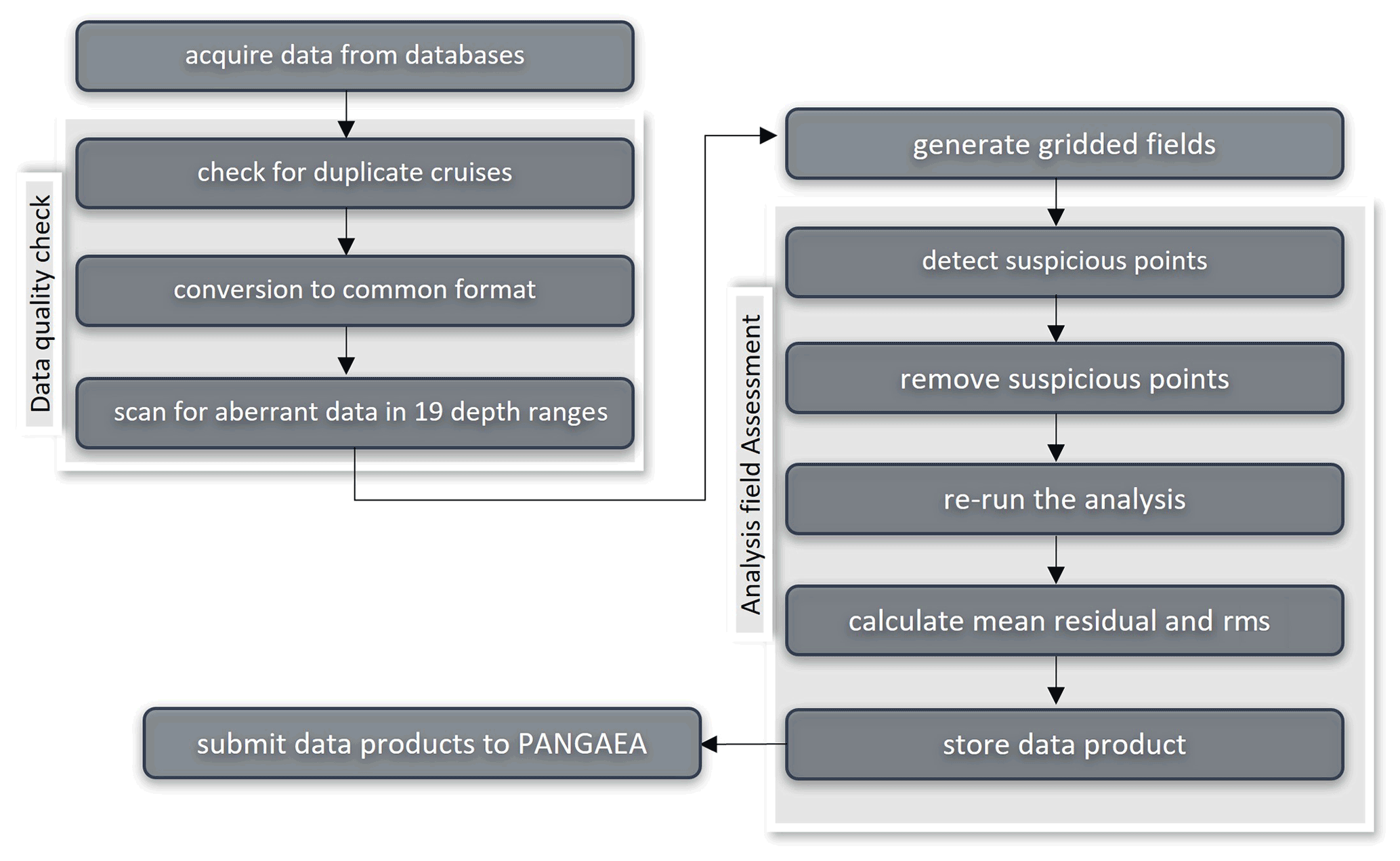
Figure 4 Flowchart describing the steps during the quality control; see text in Sects. 2.3 and 3.3 for more details.

As detailed in Table 2, we combined observations from reliable sources (covering the time period 1981–2017), which were quality controlled according to international recommendations before being published (Maillard et al., 2007; SeaDataNet Group, 2010). However, these historical data collections coming from sources different from the CNR_DIN_WMED_20042017 were subjected to a quality check before merging them to eliminate the effect of any aberrant observation. The check was carried out by computing median absolute deviations in 19 pressure classes (referring to the selected vertical resolution of Sect. 2.1, Fig. 3b) (0–10, 10–30, 30–60, 60–80, 80–160, 160–260, 260–360, 360–460, 460–560, 560–900, 900–1200, 1200–1400, 1400–1600, 1600–1800, 1800–2000, 2000–2200, 2200–2400, 2400–2600, > 2600 dbar). Any value that is more than three median absolute deviations from the median value is considered a suspect measurement.

In total, 2.35 % of nitrate observations, 2.44 % of phosphate observations and 2.14 % of silicate observations were removed.

3 Methods

3.1 Variational analysis mapping tool

Here, the Data-Interpolating Variational Analysis in N dimensions (DIVAnd) method (Beckers et al., 2014; Troupin et al., 2010, 2012) was used to generate the gridded fields. DIVA has been widely applied to oceanographic climatologies, such as the SeaDataNet climatological products (Simoncelli et al., 2014, 2016, 2019, 2020a, b, c, 2021; Iona et al., 2018), EMODnet chemistry regional climatologies (Míguez et al., 2019), the Adriatic Sea climatologies by Lipizer et al. (2014) or the Black Sea (Capet et al., 2014), and it was also applied to generate the global interior climatology GLODAPv2.2016b (Lauvset et al., 2016). It is an efficient mapping tool used to build a continuous spatial field from discrete, scattered, irregular in situ data points with an error estimate at each level.

The BGC-WMED gridded fields have been computed with the more advanced N-dimensional version of DIVA, DIVAnd v2.5.1 (Barth et al., 2014) (https://doi.org/10.5281/zenodo.3627113), using Julia as a programming language (https://julialang.org/, last access: 3 September 2019​​​​​​​) under the Jupyter environment (https://jupyter.org/, last access: 3 September 2019). The code is freely available at https://github.com/gher-ulg/DIVAnd.jl (last access: 27 January 2020​​​​​​​).

DIVA is based on the variational inverse method (VIM) (Brasseur et al., 1996). It takes into account the errors associated with the measurements and takes account of the topography/bathymetry of the study area. The method is designed to estimate an approximated field φ close to the observations and find the field that minimizes the cost function J[φ].

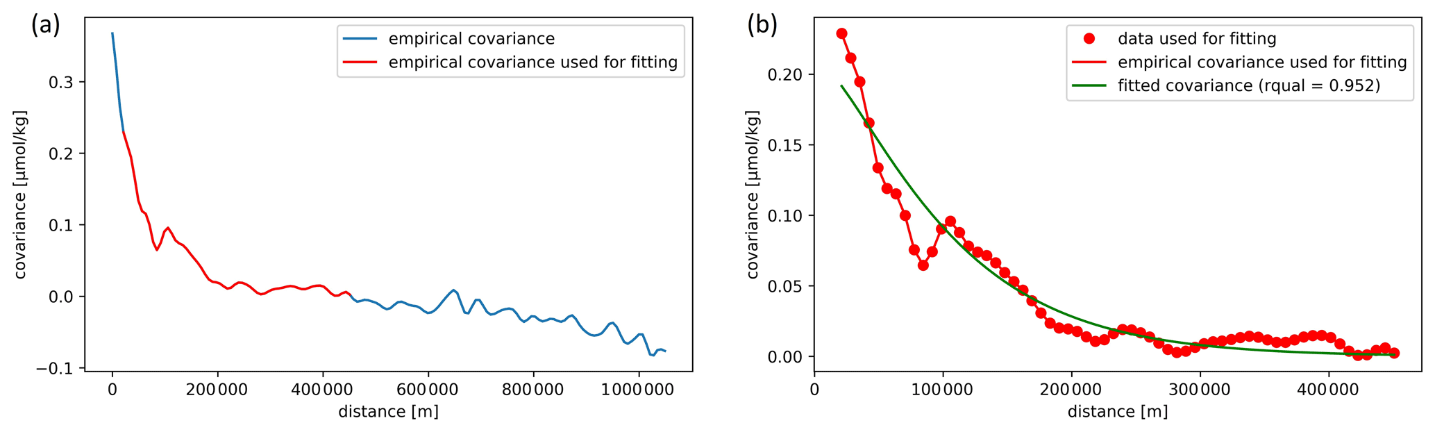
Figure 5 Example of the nitrate covariance. (a) The empirical data covariance function is given in red, and the curve comes from the analysis of observations within a depth of 10 m, while in (b) the fitted covariance curve (theoretical kernel) is given in green.

The cost function is defined as the misfit between the original data d_i, an array of N_d observations, the analysis (observation constraint term) and a smoothness term (Troupin et al., 2010):

$$\begin{array}{}\text{(1)}& \begin{array}{rl}J\left[\mathit{\phi }\right]=& \sum _{i=\mathrm{1}}^{N_{\mathrm{d}}}{\mathit{\mu }}_i{L_{\mathrm{c}}}^{\mathrm{2}}(d_i-\mathit{\phi }(x_i,y_i){)}^{\mathrm{2}}\\ & \text{(1 – observation constraint term)}\\ & +\underset{D}{\int }\left({\mathit{\alpha }}_{\mathrm{2}}\mathrm{\nabla }{\mathrm{\nabla }}_{\mathit{\phi }}:\mathrm{\nabla }{\mathrm{\nabla }}_{\mathit{\phi }}+{\mathit{\alpha }}_{\mathrm{1}}{L_{\mathrm{c}}}^{\mathrm{2}}{\mathrm{\nabla }}_{\mathit{\phi }}{\mathrm{\nabla }}_{\mathit{\phi }}+{\mathit{\alpha }}_{\mathrm{0}}{L_{\mathrm{c}}}^{\mathrm{4}}{\mathit{\phi }}^{\mathrm{2}}\right)\mathrm{d}D\\ & \text{(2 – smoothness term),}\end{array}\end{array}$$

where L_c is the correlation length, ∇ is the gradient operator, ∇∇_φ: ∇∇_φ is the squared Laplacian of φ, and the first term (observation constraint) considers the distance between the observations and the analysis reconstructed field φ(x_i,y_i) so that μ_i penalizes the analysis misfits relative to the observations. If the observation constraint were only composed of $d_i-\mathit{\phi }(x_i,y_i)$, the constructed field would be a simple interpolation of the observations and the minimum would be reached when $d_i=\mathit{\phi }(x_i,y_i)$. The field φ(x_i,y_i) needs to be close to the observation and not have large variation. The second term (smoothness term) measures the regularity of the domain of interest D. This expression within the integral remains invariant (Brasseur and Haus, 1991). α₀ minimizes the anomalies of the field itself; α₁ minimizes the spatial gradients; α₂ penalizes the field variability (regularization). The reconstructed fields are determined at the elements of a grid on each isobath using the cost function of Eq. (1).

The grid is dependent on the correlation length and the topographic contours of the specified grid in the considered region, so there is no need to divide the region before interpolating.

The method computes two- to three- to four-dimensional analyses (longitude, latitude, depth, time). For climatological studies, the four-dimensional extension was used on successive horizontal layers at different depths for the whole time period.

Along with the gridded fields, DIVA yields error fields dependent on the data coverage and the noise in the measurements (Brankart and Brasseur, 1998; Rixen et al., 2000). Full details about the approach are provided extensively by Barth et al. (2014) and Troupin et al. (2018) in the “Diva User Guide” (https://doi.org/10.5281/zenodo.836723).

3.2 Interpolation parameters

DIVAnd is conditioned by topography, by the spatial correlation length (L_c) and by the signal-to-noise ratio (SNR, λ) of the measurements, which are essential parameters to obtain meaningful results. They are considered in more detail in the following sections.

3.2.1 Land–sea mask

A 3D land–sea mask is created using the coastline and bathymetry of the General Bathymetric Chart of the Oceans (GEBCO) 30 s topography (Weatherall et al., 2015). The WMED is a relatively small area which necessitates a high-resolution bathymetry to generate a mask at different depth layers. The vertical resolution is set to 19 standard depth levels from the surface to 1500 m: 0, 5, 10, 20, 30, 50, 75, 100, 150, 200, 250, 300, 400, 500, 600, 700, 800, 1000 and 1500 m, corresponding to the most commonly used predefined levels for the sampling of seawater for nutrient analyses. The resulting fields at each depth level are the interpolation on the specified grid. These depth surfaces are the domain on which the interpolation is performed.

3.2.2 The spatial correlation length scale (L_c)

L_c indicates the distance over which an observation affects its neighbors. The correlation length can be set by the user or computed using the data distribution.

For the BGC-WMED, this parameter was optimized for the whole time span and at each depth layer. The correlation length has been evaluated by fitting the empirical kernel function to the correlation between data isotropy and homogeneity in correlations. The quality of the fit is dependent on the number of observations (Troupin et al., 2018). The analytical covariance model used in the fit is derived for an infinite domain (Barth et al., 2014). To assess the quality of the fit, the data covariance and the fitted covariance are plotted against the distance between data points (Fig. 5). At 10 m, the correlation length was obtained with a high number of data points, indicating that the empirical covariance used to estimate the covariance and the fitted covariance are in good agreement.

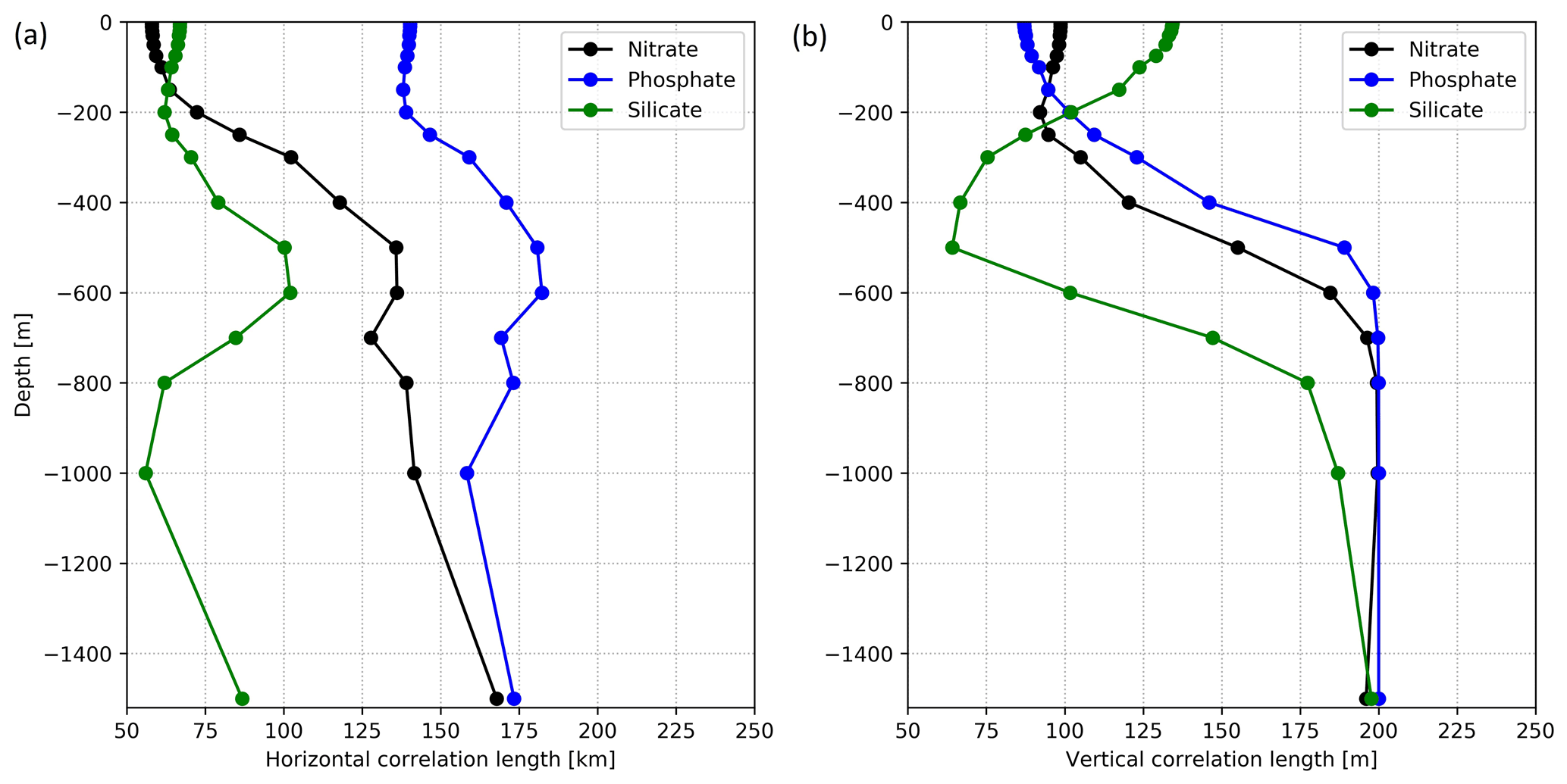
Figure 6 (a) Horizontal and (b) vertical optimized correlation lengths, for each nutrient (1981–2017), as a function of depth.

At some depth layers there are irregularities due to an insufficient number of data points, making it necessary to apply a smoothing filter/fit to minimize the effect of these irregularities. It has been tested whether a randomly selected field analysis (nitrate data from 2006 and 2015) obtained with the fitted vertical correlation profile is better than the analysis with zero vertical correlation. A skill score relative to analysis with non-fitted vertical correlation has been computed following Murphy (1988) and Barth et al. (2014):

$$\begin{array}{}\text{(2)}& \text{skill score}=\mathrm{1}-{\displaystyle \frac{{\text{rms}}_{\text{no fit}}^{\mathrm{2}}}{{\text{rms}}^{\mathrm{2}}}}.\end{array}$$

A large difference in the global rms between the analysis with the fitted vertical correlation and the analysis with non-fitted vertical correlation used for validation was found. The test shows whether the use of the fit in the correlation profile improves the overall analysis or not. We found that the RMSE (nitrate analysis of 1981–2017) was reduced from 0.696 µmol kg⁻¹ (analysis without fit) to 0.571 µmol kg⁻¹ (analysis with fit) at 10 m depth, which means using the fitted vertical correlation profile in the analysis improves the skill by 32 %, and the fit improves the analysis fields.

Based on the data, DIVA performs a least-squares fit of the data covariance function with a theoretical function. Then, a vertical filter is applied and an average profile over the whole period is used (Fig. 6). This procedure is analogous to what has been used for the EMODnet climatology and the North Atlantic climatology, except that in EMODnet climatology, seasonally averaged profiles were used (Buga et al., 2019) and monthly averaged profiles were used in North Atlantic climatology (Troupin et al., 2010). The filter is applied to discard aberration caused by outliers or scarce observations in some layers, as described above.

Because of the horizontal and vertical inhomogeneity of the data coverage, the analysis was based on a correlation length that varies both horizontally (Fig. 6a) and vertically (Fig. 6b).

As expected, L_c increases with depth (Fig. 6), extending the influence area of the observation, a consequence of the fact that variability at depth is lower and that observations in the deep layer are scarcer (which on the other hand makes the L_c estimate more uncertain).

From the surface to 150–200 m, L_c is rather constant (Fig. 6), while from 200 to 600 m, the horizontal L_c (Fig. 6a) increases for all nutrients. Below 600 m, the horizontal L_c for silicate decreases down to 1000 m and then increases again at 1500 m. For nitrate and phosphate, a similar, but less marked, behavior is observed.

The vertical L_c (Fig. 6b) behaves similarly toward the increase, for nitrate and phosphate, due to the homogeneity of the intermediate water mass, as explained also by Troupin et al. (2010). For silicate, the vertical L_c decreases in the intermediate depth, reaching a minimum at 500 m depth. The different behavior of silicate could be explained by the progressive increase in concentrations from the surface to the deep layer, compared to nitrate and phosphate vertical distribution (a strong gradient between the surface depleted layer and intermediate layer). L_c for silicate has lower values compared to nitrate and phosphate because, horizontally and vertically, it behaves in a different way. Unlike nitrate and phosphate, silicate does not show a strongly increased east–west gradient. This gradient might induce this difference in the horizontal distance over which the sample influences its neighborhood.

Besides, silicate is less utilized by primary producers, and the dissolution of the biogenic silica is slower than that of the other nutrients (DeMaster, 2002), which explains its progressive increase toward deeper layers (Krom et al., 2014). The vertical L_c for all nutrients increases progressively from 400 to 1500 m.

Troupin et al. (2010) and Iona et al. (2018) attributed similar changes observed in L_c for temperature and salinity to the variability in the water masses in each layer. This might also explain the changes found in L_c for nutrients. Indeed, the concentration of nutrients in the WMED increases with depth and is very low at the surface, which explains the constant low values of L_c in this layer.

3.2.3 Signal-to-noise ratio

The signal-to-noise ratio (SNR) is related to the confidence in the measurements. It is the ratio between the variance of the signal and the variance of the measurement noise/error. The SNR defines the representativeness of the measurements relative to the climatological fields; in other words, it is the confidence in the data.

It not only depends on the instrumental error but also on the fact that observations are instantaneous measurements, and since a climatology is a long-term mean, such observations do not represent exactly the same.

Generally, small SNR values favor large deviations from the real measurements to give a smoother climatological field. On the other hand, with a high SNR, DIVAnd keeps the existing observations and interpolates between data points. The need is to find an approximation that does not deviate much from the real observations (further details in Lauvset et al., 2016, and Troupin et al., 2010).

Following the same approach that many climatologies that used the DIVAnd method adopted, i.e., EMODnet climatologies (available on the EMODnet chemistry portal), the Atlantic regional climatologies (Troupin et al., 2010), the Adriatic Sea climatology (Lipizer et al., 2014) and the SeaDataNet regional climatology (Simoncelli et al., 2015), the SNR is set to a constant value (Table 1).

The analysis is performed with a predefined uniform default error variance of 0.5 for all parameters at all depths; we presume that the data sources used to generate the BGC-WMED are consistent products. Three iterations are performed inside DIVAnd to estimate the optimal scale factor of error variance of the observation (following Desroziers et al., 2005). More details can be found at https://gher-ulg.github.io/DIVAnd.jl/latest/#DIVAnd.diva3d (last access: 27 January 2021​​​​​​​)​​​​​​​.

Values of SNR provided by means of a generalized cross-validation (GCV) technique (Brankart and Brasseur, 1998) gave a large estimate of the SNR (of the order of 22) showing a discontinuous analysis field and patterns around the cruise transects that do not represent properly the climatological fields.

3.3 Detection of suspicious data

Assessment of the analysis is performed by detecting outliers and suspicious data in order to remove observations that generate irregular interpolated fields and suspect observations that were not detected in the data quality check of Sect. 2.3.

The automatic check measures how consistent the gridded field is, with respect to the nearby observations, by estimating the difference between a measurement and its analysis scaled by the expected error; based on that, a score is assigned to each observation. Data points with the highest scores were considered suspect and were removed from the analysis (Figs. B1–B3). Overall, 0.031 %, 0.014 % and 0.004 % of data points for nitrate, phosphate and silicate, respectively, were considered inconsistent. Details about the quality check values and range are plotted in Appendix B (Table B1).

Figure 7 Vertical mean residuals (in red), i.e., the differences between the observations and the analysis, and the mean rms (dashed blue) of (a) nitrate, (b) phosphate and (c) silicate.​​​​​​​

3.4 Quality check of the analysis fields

The quality of the climatology was checked against observations by estimating the mean residual and the root mean square (rms) of the difference between the climatology and the observations. Averages over the entire basin were calculated between depth surfaces (see Sect. 2.3). Residuals are the difference between the observations within the specific depth surface and the analysis (interpolated linearly to the location of the observations) and are estimated by depth range (Fig. 7). The analysis fields at each depth range (i.e., depth surfaces or domain on which the interpolation is performed) are the interpolation on the specified grid. In Fig. 7, we present the vertical profile of the mean residuals and rms at different depth ranges for the three nutrients.

Nitrate observations and the analysis field in Fig. 7a have a high level of agreement in the surface layer (from 0 to 30 m depth). Just below (between 30 and 200 m), boxplots are suggestive of larger differences. From the surface to the deep layer, the mean residual between nitrate observation and the gridded field varied between −0.075 and 0.0765 µmol kg⁻¹, while the corresponding rms fluctuated between 0.47 and 1.1 µmol kg⁻¹. This is justified by the inhomogeneity of the observations mainly in deep layers.

As for the average residual between phosphate observations and the gridded analysis (Fig. 7b), it was around zero and varied between −0.0027 and 0.0026 µmol kg⁻¹. The rms for phosphate was between 0.037 and 0.063 µmol kg⁻¹.

Silicate residuals (Fig. 7c), on the other hand, seemed more homogeneous at all depth levels. The highest level of agreement was found below 20 and at 600 m. Overall, residuals varied between −0.057 and 0.063 µmol kg⁻¹, while the rms ranged between 0.567 and 0.963 µmol kg⁻¹.

Over the entire water column, the mean residual was around zero (0.004 µmol kg⁻¹ for nitrate, 0.0002 µmol kg⁻¹ for phosphate and 0.003 µmol kg⁻¹ for silicate) (Fig. 7). The rms (blue line) fell within the mean residual ± standard deviation in the upper 25th percentile at the different depth ranges and in all parameters, meaning that, in general, the bias between the observations and the analysis is small and there is a good agreement.

4 Results

The final result consists of gridded fields of mapped climatological means of inorganic nutrients for the periods 1981–2004 and 2005–2017 and the whole period of 1981–2017, produced with the VIM described in Sect. 3, using data of Sect. 2. Together with the gridded fields, error maps have been generated to check the degree of reliability of the analysis.

Table 3 Available analyzed fields and related information in the netCDF files.

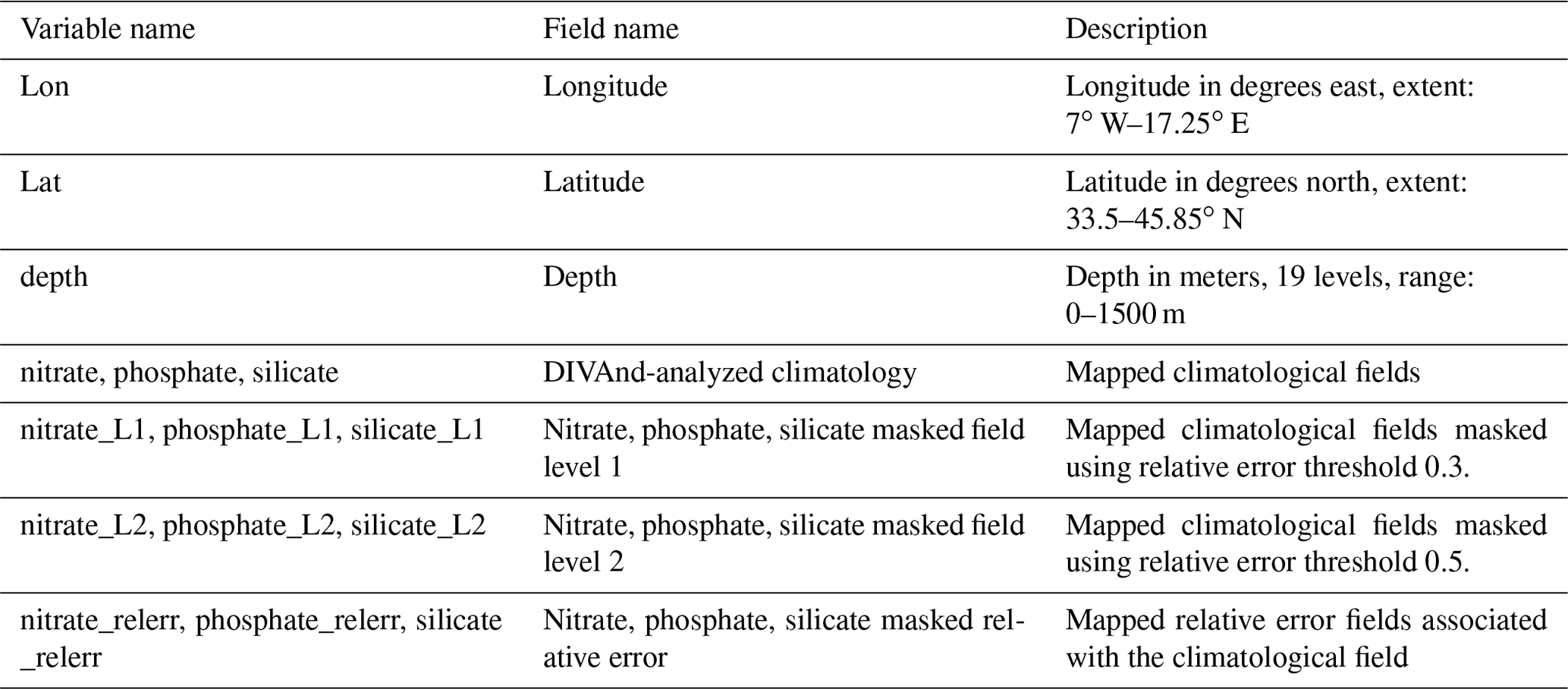
The resulting climatologies (Table 3) are aggregated in a 4D netCDF for each nutrient and each time period that contains the interpolated field of the variable and the related information: associated relative error and variable fields masked using two relative error thresholds (L1 and L2). The mapped climatology is available from PANGAEA (https://doi.org/10.1594/PANGAEA.930447, Belgacem et al., 2021) as one folder named BGC-WMED climatology. This folder contains nine files: three per parameter and three per time period.

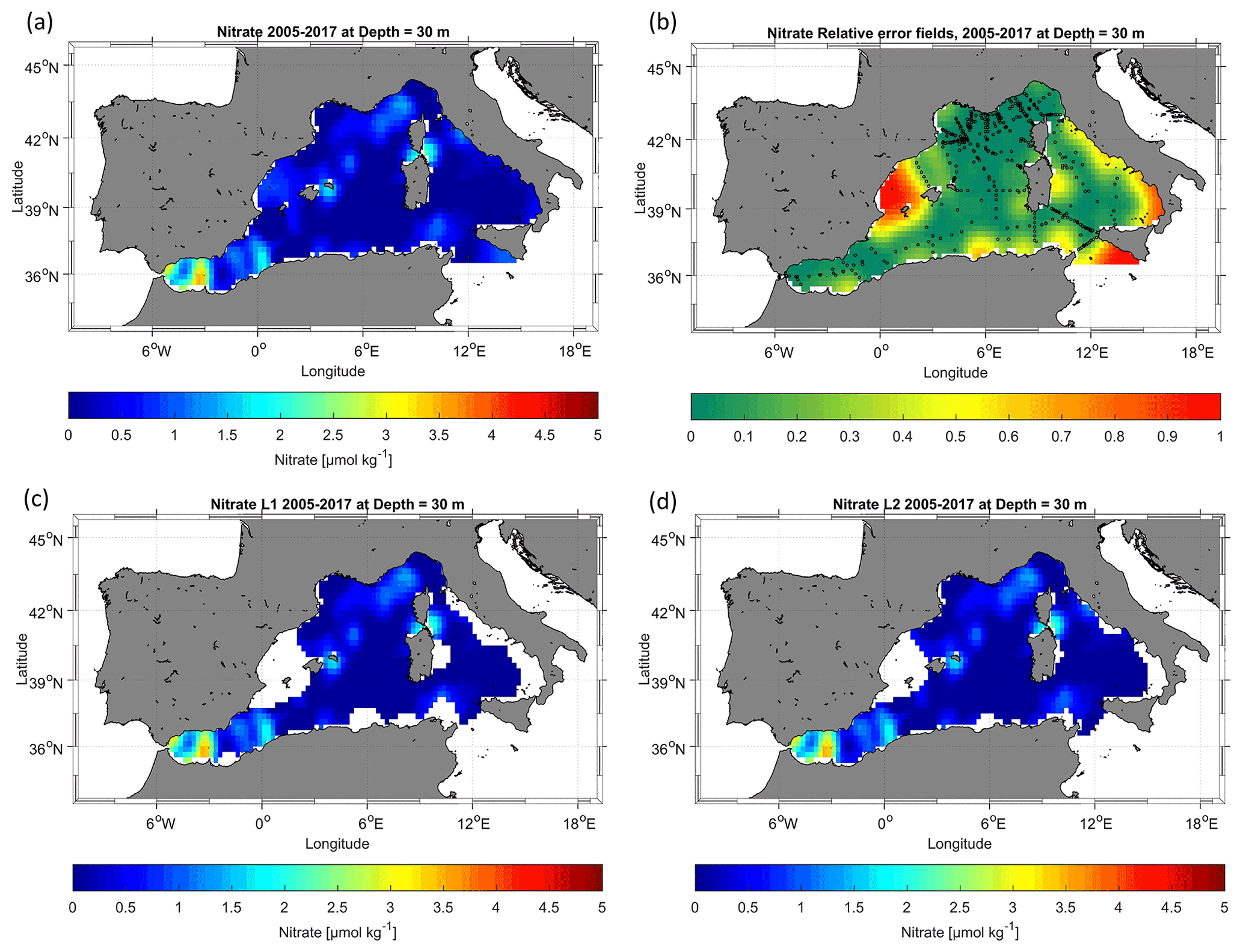
Figure 8 Example of nitrate analysis for the period 2005–2017: (a) unmasked analysis field, (b) relative error field distribution with the observation in black circles, (c) masked analysis fields masked using a relative error threshold of 0.3 and (d) masked analysis fields masked using a relative error threshold of 0.5.

Figure 8 shows an example of the analysis output found in the netCDF. It shows the unmasked climatological field of the mean spatial variation in nitrate, the relative error field distribution and the masked climatological field using relative error with two threshold values (0.3 and 0.5) to assess the quality of the resulting fields.

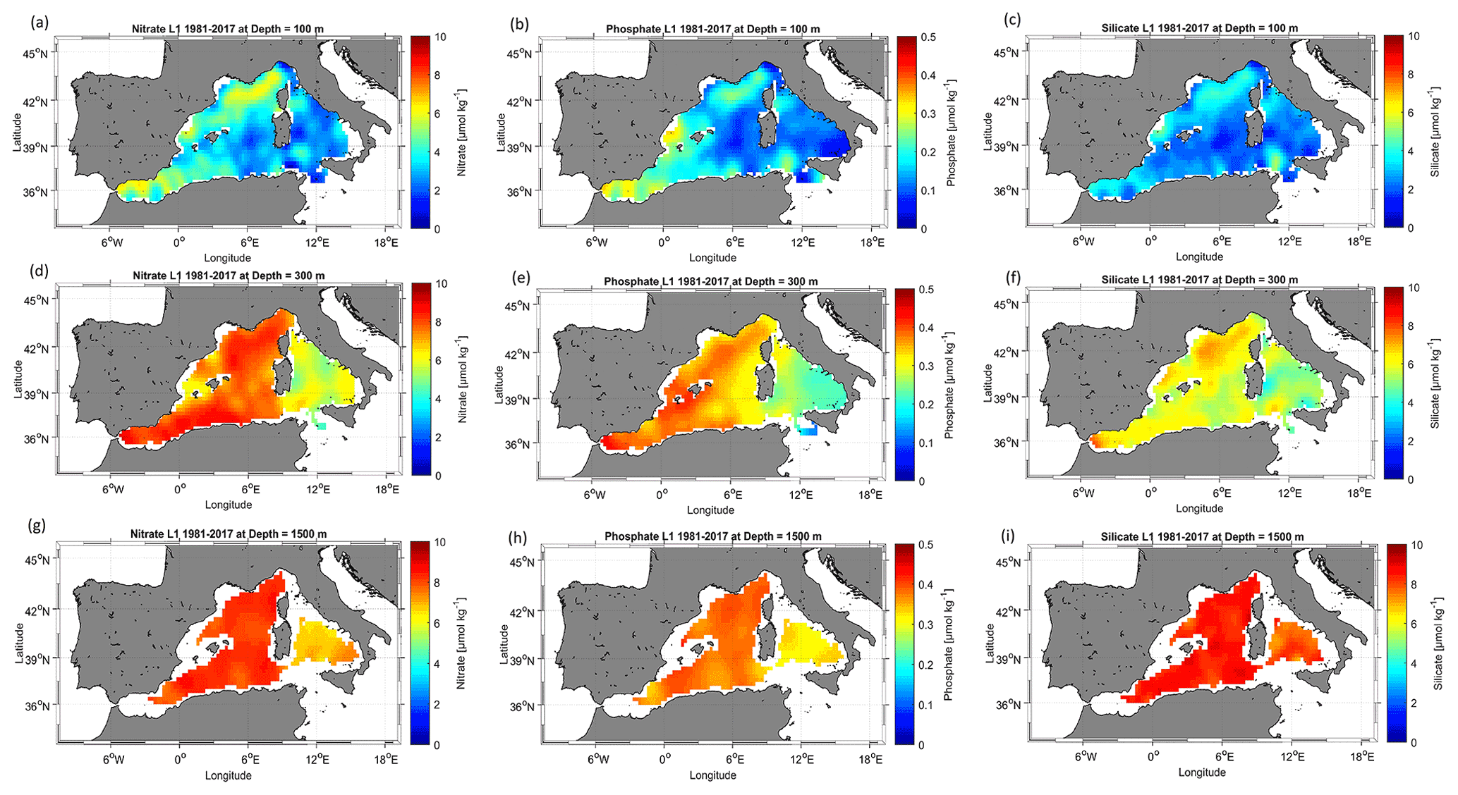
Figure 9 Climatological map distribution of nitrate (a at 100 m, d at 300 m, g at 1500 m), phosphate (b at 100 m, e at 300 m, h at 1500 m) and silicate (c at 100 m, f at 300 m, i at 1500 m) for the period from 1981 to 2017.

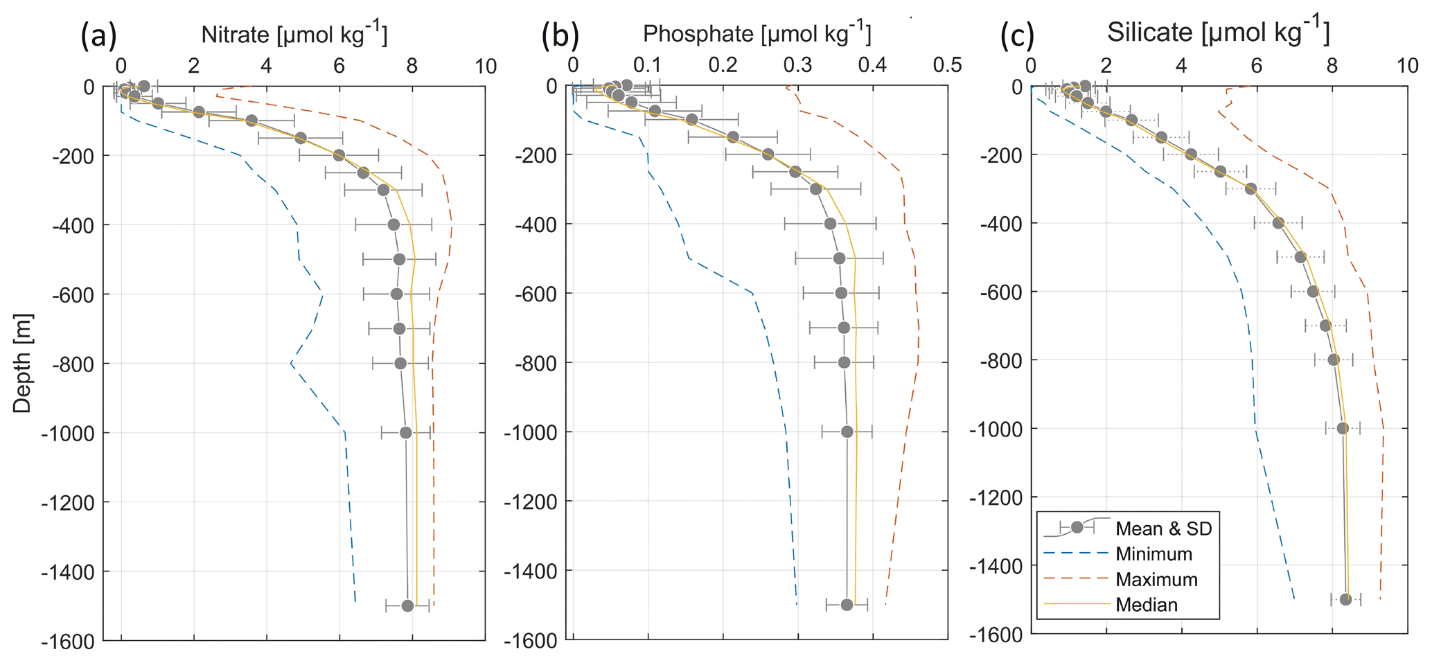
Figure 10 Climatological mean vertical profiles of (a) nitrate, (b) phosphate and (c) silicate concentrations in the WMED (1981–2017). The dashed blue line indicates the minimum; the dashed orange line indicates the maximum; the solid yellow line indicates the median profile; error bars and the mean profile are in grey.

4.1 Nutrient climatological distribution

A description of the spatial patterns of the dissolved inorganic nutrients across the domain and over the entire period (1981–2017) is given. The gridded fields for nitrate, phosphate and silicate are discussed at three depth levels, representative of the surface (at 100 m), intermediate (at 300 m) and deep (at 1500 m) layer. The horizontal maps at the selected depths are shown in Fig. 9, while the average vertical profiles of nutrients over the whole area are shown in Fig. 10.

4.1.1 Surface layer

The nitrate, phosphate and silicate mean climatological fields over 1981–2017 are presented in Fig. 9a–c, respectively. The mean surface nitrate at 100 m is about 3.58 ± 1.16 µmol kg⁻¹. The highest surface values of nitrate concentrations are found in regions where strong upwelling or vertical mixing occurs, such as the Liguro-Provençal basin and the Alboran Sea (see Fig. 9a), and regions with extensive supply by the Ebro, Rhône, Moulouya and Chelif rivers.

The convection region (Gulf of Lion and Ligurian Sea) is characterized by a eutrophic regime and a spring bloom (Lavigne et al., 2015), unlike the rest of the basin, which shows low nitrate concentrations in the surface layer (< 4 µmol kg⁻¹).

Nutrient patterns in the Alboran Sea have been associated with the distinct vertical mixing that supplies the surface layer with nutrients (Lazzari et al., 2012; Reale et al., 2020).

Indeed, the northern Alboran Sea is known as an upwelling area, where permanent strong winds enhance the regional biological productivity (Reul et al., 2005). The nitrate distribution at 100 m presents a clear distinction between the enriched surface regions in the WMED, under the influence of deep convection processes, and the easternmost depleted regions.

The distribution of phosphate concentration has striking similarities with that of nitrate (Fig. 9b). The mean surface phosphate concentration at 100 m is 0.16 ± 0.06 µmol kg⁻¹. As for nitrate, the highest surface values are found in the Alboran Sea, Balearic Sea, Gulf of Lion and Liguro-Provençal Basin (0.2–0.3 µmol kg⁻¹), while the Tyrrhenian Sea and the Algerian Sea revealed phosphate concentrations that were < 0.2 µmol kg⁻¹. Similar patterns were observed by Lazzari et al. (2016), who argued that the variations in phosphate are regulated by atmospheric and terrestrial inputs. It should be noted that the maximum in the surface is found near river discharges of freshwater, like those of the Ebro and Rhône, i.e., the largest rivers of the WMED (Ludwig et al., 2009).

Concerning the distribution of silicate concentration, the surface layer at 100 m (Fig. 9c) followed the same pattern as those of nitrate and phosphate. Over this layer the mean silicate was about 2.7 ± 0.7 µmol kg⁻¹. As for nitrate and phosphate, the highest values (3–4 µmol kg⁻¹) were recorded in the Alboran Sea, Balearic Sea, Gulf of Lion and Liguro-Provençal Basin and at the southern entrance of the Tyrrhenian Sea. This surface distribution is in good agreement with the findings of Crombet et al. (2011), relating this local silicate surface maximum to the continental input, river discharge and atmospheric deposition (Frings et al., 2016; Sospedra et al., 2018). The spatial minima were reported in the Tyrrhenian Sea and in the Algerian Sea (< 3 µmol kg⁻¹).

4.1.2 Deep and intermediate layer

At the basin scale, nitrate concentrations increase with depth (Fig. 10a), with the highest concentration found at intermediate levels (250–500 m), ranging between 8.8 and 9.0 µmol kg⁻¹. In this 300 m layer (Fig. 9d), the nitrate concentration average is 7.2 ± 1.06 µmol kg⁻¹. High values (> 6.5 µmol kg⁻¹) are found in the westernmost regions (Alboran Sea, Algerian Sea, Gulf of Lion, Balearic Sea and Liguro-Provençal Basin), while the easternmost regions (Tyrrhenian Sea, Sicily Channel) exhibit much lower concentrations (between 4.5 and 6.5 µmol kg⁻¹).

Similar features are observed in the deep layer, at 1500 m (Fig. 9g), with nitrate concentrations increasing all over the basin, reaching on average 7.8–7.9 µmol kg⁻¹ between 1000 and 1500 m depth (Fig. 10a).

In both layers (300 and 1500 m), the difference between the eastern opening of the basin (Sicily Channel) and the western side (Alboran Sea) is noticeable: the Sicily Channel and the Tyrrhenian Sea are under the direct influence of the water masses coming from the oligotrophic EMED, which then gradually become enriched with nutrients along their paths, as found by Schroeder et al. (2020).

Phosphate concentrations at intermediate depth (see 300 m, Fig. 9e) varied between 0.12 and 0.44 µmol kg⁻¹, and the horizontal map shows the same gradual decrease toward the east, with the highest concentrations in the westernmost regions and minimum values in the eastern regions (< 0.25 µmol kg⁻¹).

The average vertical profile over the entire region (Fig. 10b) reveals a maximum in phosphate concentrations between 300 and 800 m depth, related to an increased remineralization process.

In the deep layer (see 1500 m, Fig. 9h), the phosphate concentration average is 0.36 ± 0.02 µmol kg⁻¹. Generally, the deep layer is homogeneous (Fig. 10b). The difference observed between the westernmost regions and the Tyrrhenian Sea remains, though the latter demonstrates higher phosphate concentrations (∼ 0.3 µmol kg⁻¹). This variation could be due to the difference in the water masses. The IW inflow from the EMED brings relatively young waters that are depleted in nutrients, while the higher concentrations in the deep layer are signatures of the older resident DW of the Tyrrhenian Sea. The change in the biological uptake in the intermediate source water could explain the regional variability in nutrients. The low productivity (D'Ortenzio and Ribera d'Alcalà, 2009) and the pronounced oligotrophic regime of EMED water (Lazzari et al., 2016) may justify the increase in nutrients in the IW.

The silicate concentration distribution at intermediate (300 m, Fig. 9f) and deep (1500 m, Fig. 9i) layers were as expected, showing a notable increase compared to the surface. Here, the silicate average concentration is 5.83 ± 0.66 µmol kg⁻¹. The maximum values were observed below 800 m: > 8.034 µmol kg⁻¹ (Fig. 10c). At 1500 m, the silicate distribution is homogeneous all over the basin (on average 8.35 ± 0.39 µmol kg⁻¹).

Generally, primary producers do not require silicate for their growth as much as they need nitrate and phosphate, which explain the disparity between nutrients patterns. Furthermore, at intermediate levels, the water is warmer than at deep levels, enhancing the dissolution rate and the progressive increase in silicate (DeMaster, 2002). The biogenic silicate is exported to greater depths and continues to dissolve, generating inorganic silicate as it sinks to the bottom. The recycling of silicate within the deep-sea sediments is later on redistributed by the deep currents which explain the homogenous horizontal distribution over the entire basin.

Comparing the three nutrients at the same depth levels, at the surface (100 m) it appears that they all show a local surface maximum, depending on local events such as strong winds, local river discharge and vertical mixing (Ludwig et al., 2010).

In the easternmost areas, the surface depletion in nutrients (Van Cappellen et al., 2014) is attributed to the variation in the thermohaline properties that has impacted primary production (Ozer et al., 2017) and the export of organic matter to intermediate and deep layers leading to the accumulation of nutrients in these depth ranges.

The Tyrrhenian Sea is not directly connected to convection regions. Here, the EMED water inflow plays a major role. Li and Tanhua (2020) found increased ventilation of the intermediate and deep layers during 2001 to 2018 in the Sicily Channel and a constant apparent oxygen utilization (AOU) between 2001–2016, suggesting constant ventilation that explains the peculiar nutrient distribution in that area. On the western side of the WMED, intermediate and deep layers exhibit an increase in nutrients. Schroeder et al. (2020) explained this increase in nitrate and phosphate at the intermediate layer with the increase in the remineralization rate at these depths along the path of IW.

The deficiency of inorganic nutrients is explained by the effect of the anti-estuarine circulation, with the IW coming from the EMED, which is known to be poor in nutrients (Krom et al., 2014; Schroeder et al., 2020), accumulating nutrients along its path. Thus, this relatively nutrient-rich Mediterranean outflow is lost to the Atlantic Ocean.

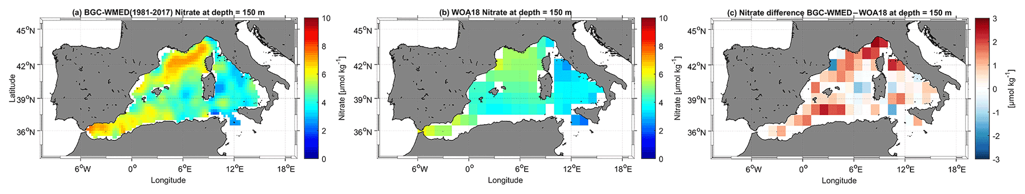
Figure 11 (a) BGC-WMED (1981–2017) nitrate climatological field at 150 m depth; (b) WOA18 nitrate climatological field at 150 m depth; (c) difference between BGC-WMED and WOA18 nitrate fields at 150 m.

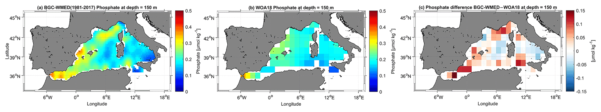
Figure 12 The same as Fig. 11 but for phosphate.

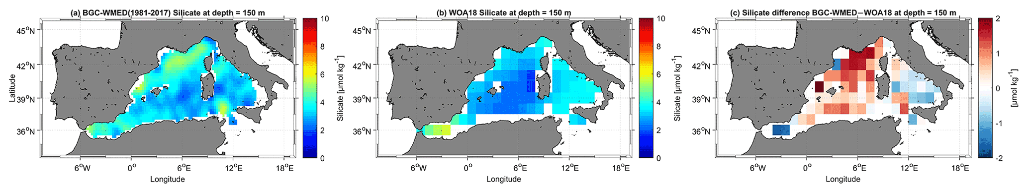
Figure 13 The same as Fig. 11 but for silicate.

Overall, in the surface layer, circulation, physical processes and vertical mixing increase nutrient input while the biological pump controls the decrease.

In the deep layer, the variability is lower (standard deviation is reduced toward the bottom for all three nutrients; see Fig. 10); the deep layer accumulates dissolved organic nutrients. In the WMED, the deep layer constitutes a reservoir of inorganic nutrients.

4.2 Error fields

The determination of the error field is important to gain insight into the confidence in the climatological results. Mostly, the error estimate depends on the spatial distribution of the observations and the measurement noise. In DIVAnd, there are different methods available to estimate the relative error associated with the analysis fields.

A climatological field is computed at several depths (19 levels in this case), for different parameters (nitrate, phosphate and silicate in this case). Given these premises and following the approach of similar climatologies (GLODAPv2.2016b, Lauvset et al., 2016; SeaDataNet aggregated dataset products, Simoncelli et al., 2015), for the BGC-WMED the error fields were estimated using the default DIVAnd method, i.e., the “clever poor man's error approach”, a less time-consuming but efficient computational approach. According to Beckers et al. (2014), who also provide details about the mathematical background of the error field computation, this method appropriately represents the true error and provides a qualitative distribution of the error estimate. This estimate is used to generate a mask over the analysis fields. Two error thresholds were applied (0.3 (L1) and 0.5 (L2)). Figure 8b shows the main error that occurs in regions void of measurements. An example of the analysis masked with the error thresholds output is shown in Fig. 8c (L1) and Fig. 8d (L2). The associated error fields with the analysis fields are integrated into the data product.

4.3 Comparison with other biogeochemical data products

In this section, a comparison of the BGC-WMED product with the most known global and/or regional climatologies that are frequently used as reference products for initializing numerical models is made.

Specifically, the analyzed fields are compared to the reference data products of the WOA18 (Garcia et al., 2019), a large-scale illustration of nutrient distribution computed by objective analysis using the World Ocean Database 2018 (Boyer et al., 2018). The new product is also compared to the reanalysis of the Mediterranean Sea biogeochemistry, MedBFM, a CMEMS product that assimilates satellite and Argo data and includes terrestrial inputs of nitrate and phosphate from 39 rivers (Teruzzi et al., 2019).

Since the products used for inter-comparison were not originated from the same interpolation method or for the same time period and have different spatial resolutions, here the comparison is mostly targeted on the general patterns of nutrients in the region.

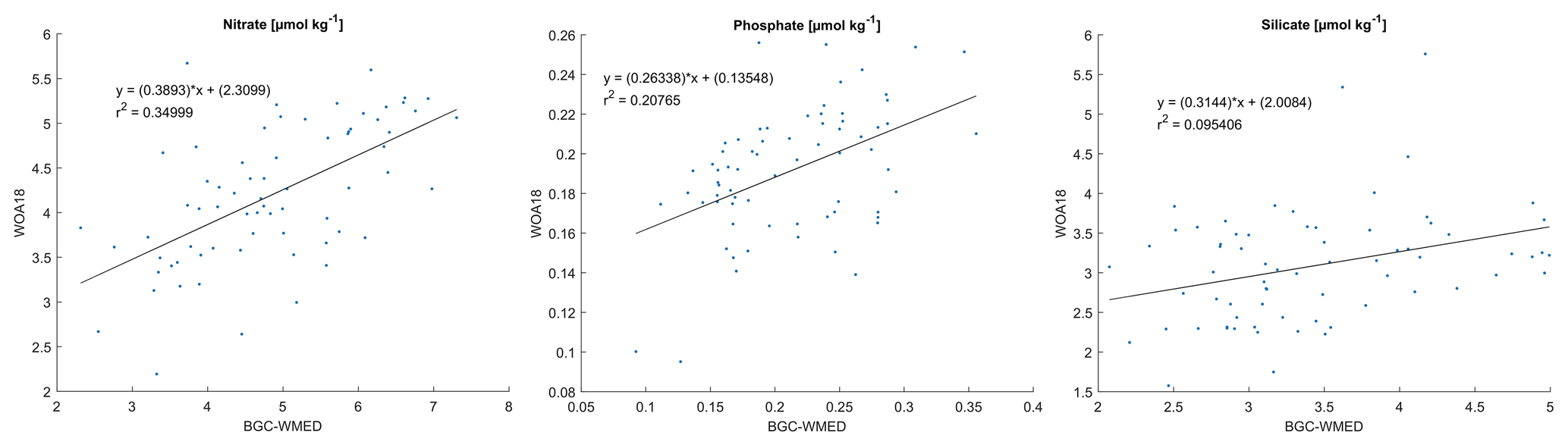
Figure 14 Scatterplot showing the WOA18 data as a function of the BGC-WMED at 150 m with the regression line.

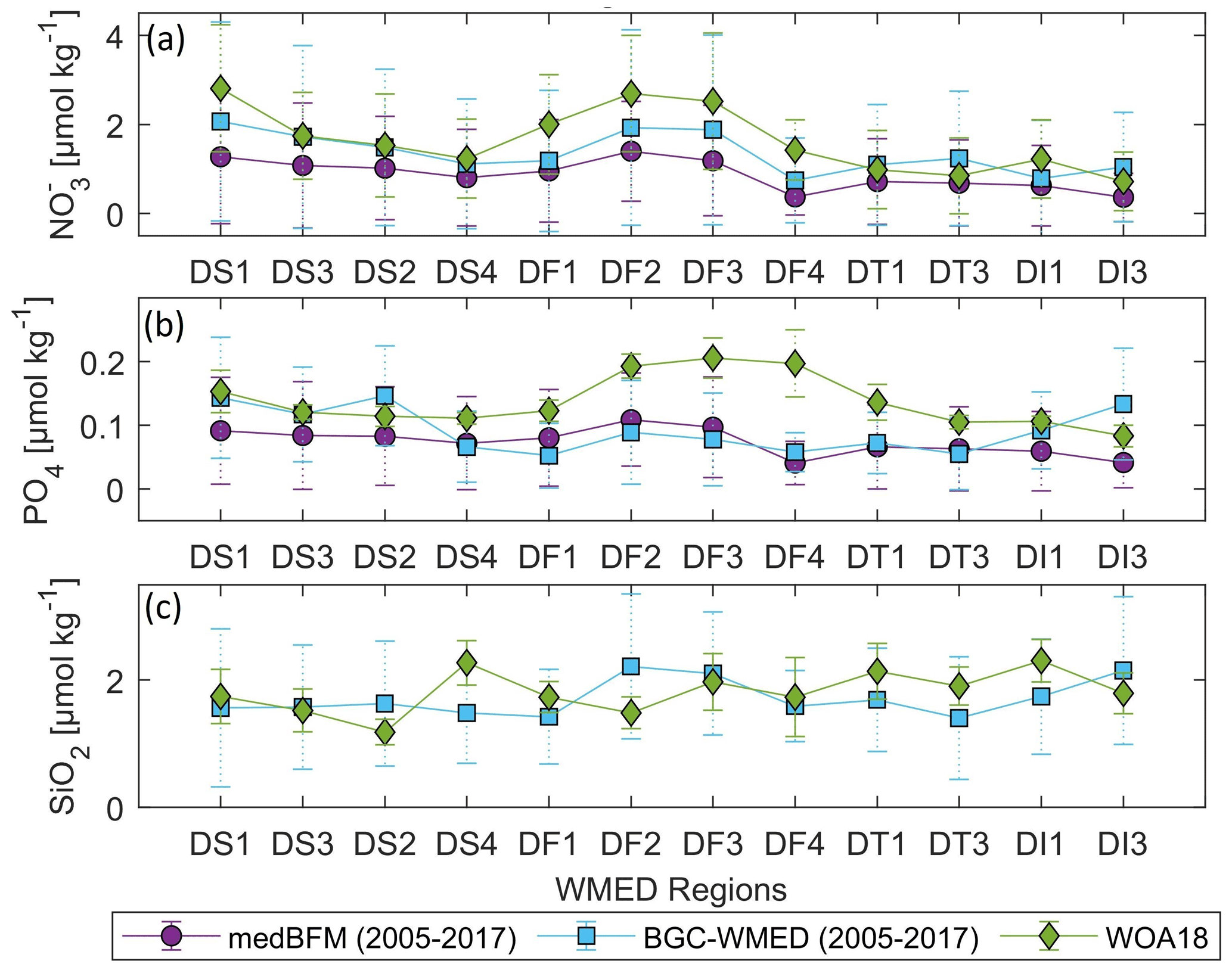
Figure 15 Nutrient average concentrations and standard deviation comparison in the upper 150 m (values in Table 4).

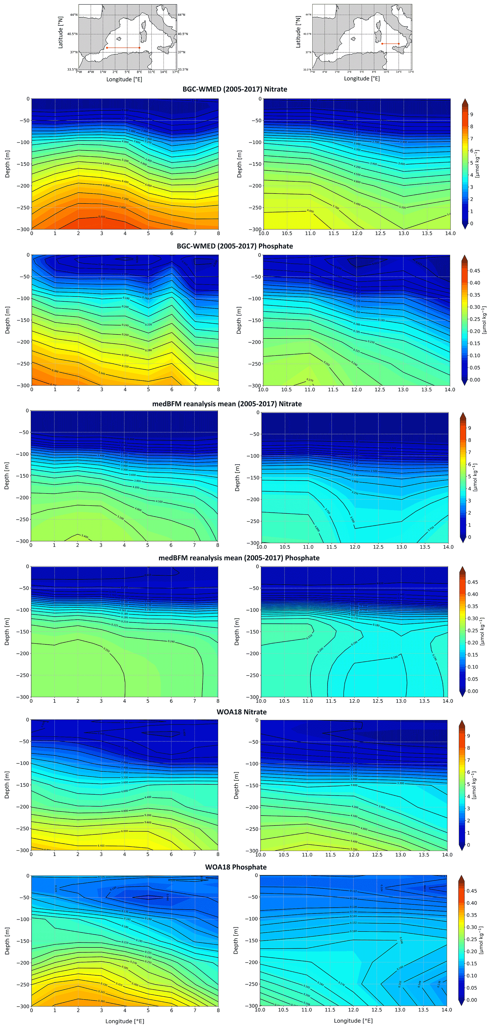
Figure 16 Vertical distribution of nitrate and phosphate from the Algerian Basin and Tyrrhenian Sea. Colors show the gridded values from the three different products: BGC-WMED, MedBFM reanalysis (Teruzzi et al., 2019) and the WOA18 (Garcia et al., 2019).

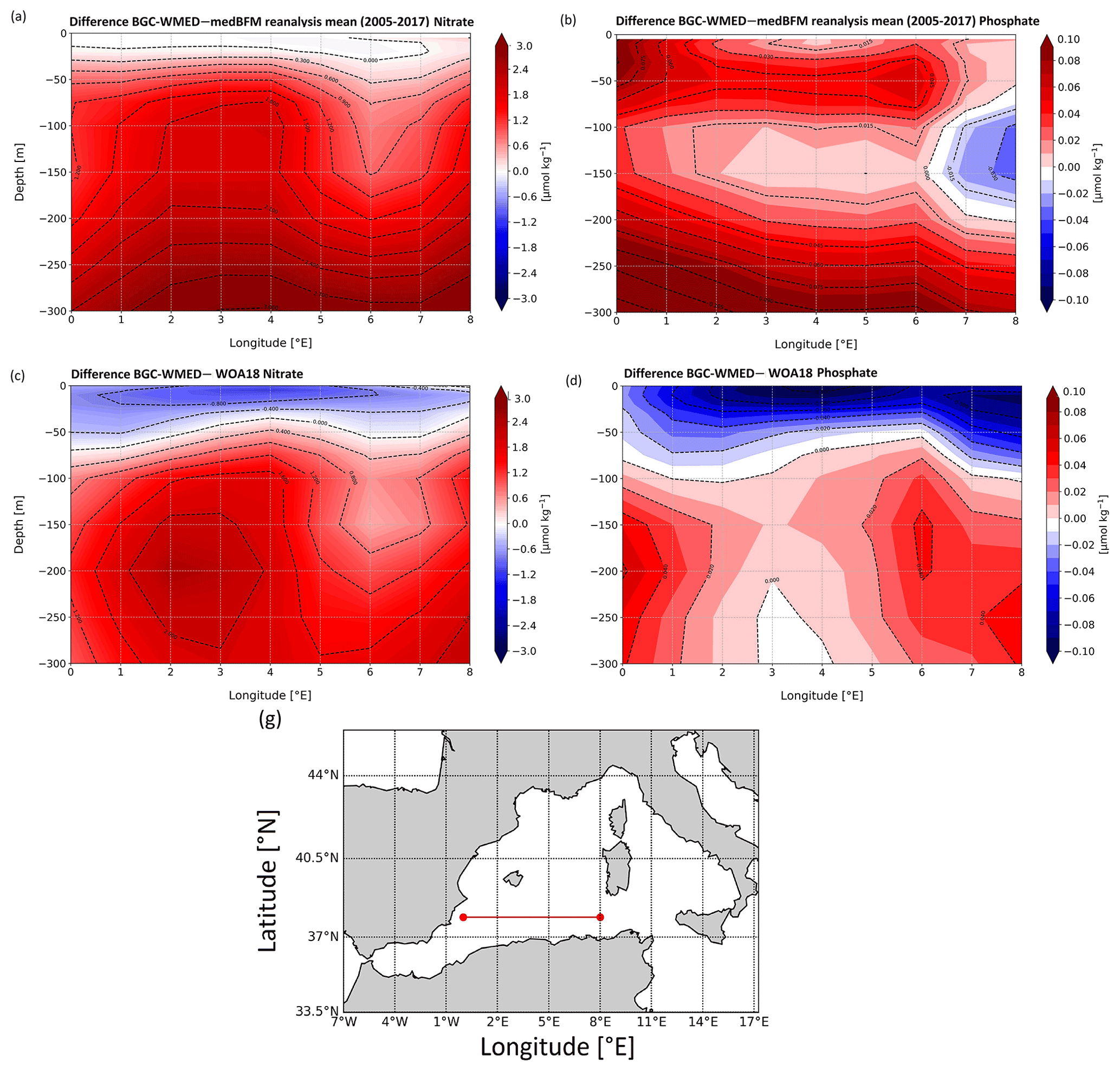
Figure 17 Difference in the vertical section from the Algerian Basin between the BGC-WMED and MedBFM (a nitrate, b phosphate) and BGC-WMED and WOA18 (c nitrate, d phosphate), with dashed contour lines and labels.

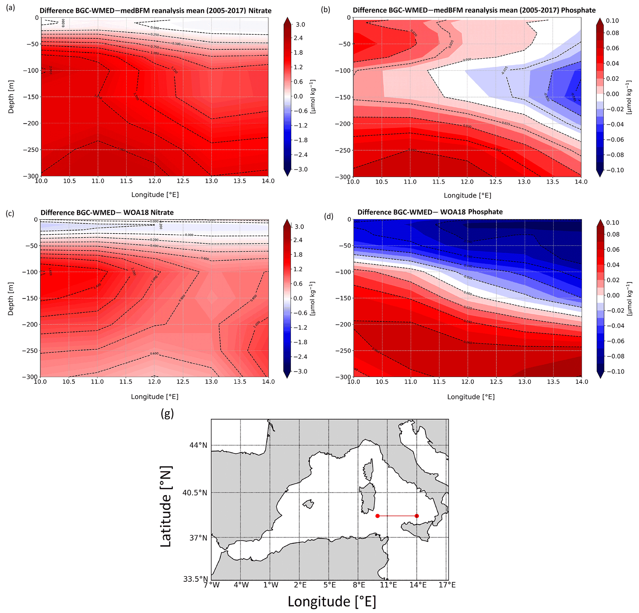
Figure 18 Same as Fig. 17 but for the vertical section from the Tyrrhenian Sea.

Comparisons are carried out between horizontal maps (Figs. 11–13), as well as along a vertical longitudinal transect (Figs. 16–18). In addition, following Reale et al. (2020), the first 150 m has been evaluated (Figs. 14 and 15) since this is a depth level with a representative number of in situ observations in all three products. The evaluation is based on the estimation of the horizontal average, the BGC-WMED, the MedBFM biogeochemical reanalysis and the WOA18 climatology by subregion. i.e., a spatial subdivision made according to Manca et al. (2004).

Products have a different grid resolution; thus to compare them and combine variables on a compatible grid, the new BGC-WMED climatological data product (at 0.25^∘ × 0.25^∘) for the periods 1981–2017 and 2005–2017 and the MedBFM biogeochemical reanalysis (at 0.063^∘ × 0.063^∘) (Teruzzi et al., 2019) (https://doi.org/10.25423/MEDSEA_REANALYSIS_BIO_006_008) for the period 2005–2017 are regridded on the WOA18 (1^∘ × 1^∘) grid, changing the resolution of the existing grid to facilitate the comparison of the transect from each product.

The regridding is computed at all depth levels of the different products using nearest-neighbor interpolation. Prior to the interpolation, the MedBFM reanalysis of nitrate and phosphate have been averaged across the period 2005–2017.

We then calculated spatial maps of the mean difference at 150 m between the new climatology and the reference products, and then an average across subregions was determined.

4.3.1 Comparison with the WOA18 at 150 m

Figures 11–13 show the analysis at the 150 m depth surface for the three nutrients. The BGC-WMED (1981–2017) product reveals detailed aspects of the general features of nitrate (Fig. 11a), phosphate (Fig. 12a) and silicate (Fig. 13a).

For the three nutrients, the new product reproduces patterns similar to the WOA18 all over the region. It shows well-defined fields and higher values of nitrate and phosphate concentrations. In the new product, nitrate concentrations varied between 2.31–7.3 µmol kg⁻¹, the WOA18 values were 2.19–5.99 µmol kg⁻¹. Phosphate ranges were similar between the two products (0.092–0.35 µmol kg⁻¹ (BGC-WMED) and 0.095–0.35 µmol kg⁻¹ (WOA18)). Likewise, silicate range values at 150 m were not different (2.07–4.99 (BGC-WMED) and 1.57–5.75 µmol kg⁻¹ (WOA18)).

The average rms difference (RMSD) calculated from the difference between the WOA18 and the BGC-WMED all over the region at 150 m is about 1.14 µmol kg⁻¹ for nitrate (Fig. 11c), 0.055 µmol kg⁻¹ for phosphate (Fig. 12c) and 0.91 µmol kg⁻¹ for silicate (Fig. 13c). Overall, the RMSE values were low, indicating limited disparity between the two products.

The difference field for every grid point reflects this discrepancy and shows areas with limited agreement between the two products that can have a difference of > 2 µmol kg⁻¹ for nitrate (Fig. 11c), > 0.1 µmol kg⁻¹ for phosphate (Fig. 12c) and > 1.5 µmol kg⁻¹ for silicate (Fig. 13c). This dissimilarity is also noted with the low r² (Fig. 14) (0.34, 0.20 and 0.095 for nitrate, phosphate and silicate, respectively)

The distribution of the surface nitrate concentrations (at 150 m) (Fig. 11a) of the new product is similar to that shown in the WOA18 (Fig. 11b). The largest difference between the two products occurs in northwest areas and in the Alboran Sea (Fig. 11c), areas of higher concentrations with more nutrient-rich surface water as described in Sect. 4.1. The difference is pronounced in these regions likely because of the occurrence of upwellings along the African coast and seasonal vertical mixing in the northern WMED, contributing to the upload of nutrients to the surface which could explain the high nitrate and phosphate concentration in the BGC-WMED. The WOA18 maps show weaker values of nutrient concentrations compared to the new product, which does not mean that there are fewer physical drivers, but it might indicate that the new product holds more in situ observations than the WOA18 in the WMED.

Phosphate surface concentrations (Fig. 12) show similar differences to those of nitrate. The largest difference with the surface phosphate of the WOA18 is found in the Alboran Sea, northern WMED and Sicily region (Fig. 12c).

As for silicate, the surface distribution shows large differences (Fig. 13c). The highest values are observed in the northwest area of the new product and in the Alboran Sea in the WOA18 climatology; this again accounts for the data coverage difference.

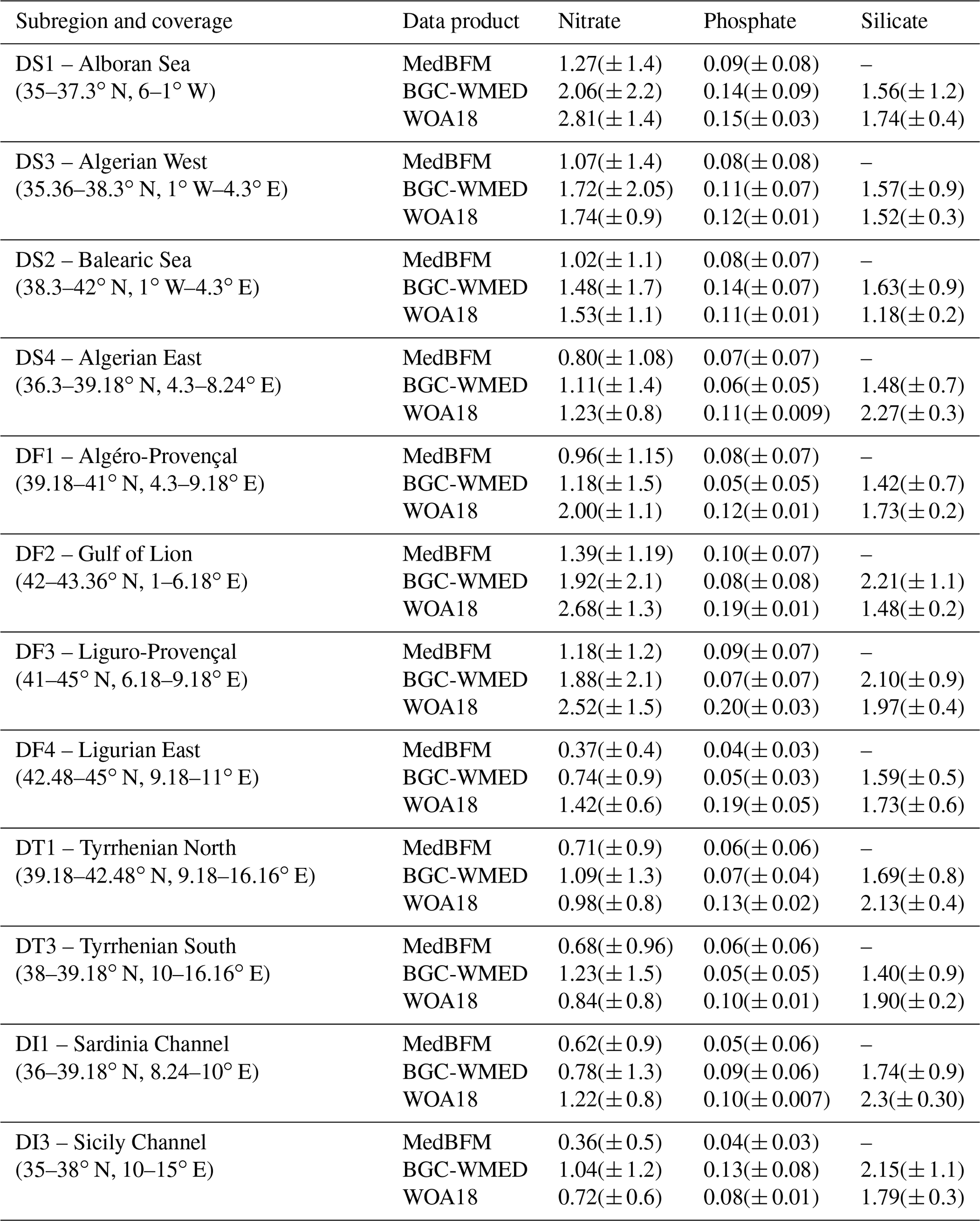
Table 4 Nutrient average concentrations and standard deviation in the upper 150 m. All products were interpolated at a 1^∘ grid resolution (see Fig. S2 in the Supplement; Belgacem et al., 2020).

4.3.2 Regional horizontal comparison above 150 m average nutrient concentrations

The inorganic nutrient mean concentrations resulting from the climatology of this work (period 2005–2017) and from both the MedBFM reanalysis product and the WOA18 are compared in the upper layer of 12 subregions of the WMED (in Table 4 and Fig. 15, including definitions of the subregion codes in Table 4).

Results show a general agreement between the BGC-WMED and the other two products in some subregions; nonetheless, there are some differences as shown in Sect. 4.3.1.

Upper-layer nitrate average concentrations (Fig. 15a) decrease eastward, from the Alboran Sea (DS1) to the Algerian Basin (DS3, DS4) and the Balearic Sea (DS2). The western part of the basin is an area under the direct influence of the inflowing Atlantic surface waters, where nitrate is known to be present in excess compared to phosphate, probably due to atmospheric N₂ input (Lucea et al., 2003). In DS1, BGC-WMED nitrate levels are lower than the WOA18 nitrate levels, while in DS3, DS2 and DS4 the average nitrate concentrations are similar to those of the WOA18.

From the Algerian Basin (DS4, DF1) to the Liguro-Provençal (DF3) regions, there is an increase in the average nitrate in all products; this is the south–north gradient. Some differences arise where the new product is lower than the WOA18.

In the eastern regions, the lowest average concentrations of the WMED are found. Here, the difference between products is smaller, with MedBFM reanalysis being lower the new product and the WOA18.

As for phosphate (Fig. 15b), known to be the limiting nutrient of the WMED, because it is rapidly consumed by phytoplankton (Lucea et al., 2003), its average levels are low in DS1, DS3, DS2 and DS4, in the WOA18, MedBFM reanalysis and BGC-WMED. The latter product did not agree well with the other products in DS2, where it was slightly higher. Phosphate average concentrations slightly increase in DF1, DF2 and DF3 in all three products. The increase is explained by the vertical mixing process occurring in the northern WMED.

Upper-surface phosphate concentration averages start to decrease progressively through the Ligurian East (DF4), Tyrrhenian Sea (DT1, DT3), Sardinia Channel (DI1) and Sicily Channel (DI3). The BGC-WMED was in agreement with MedBFM reanalysis in those subregions aside from concentrations in DI3, where the new product showed higher levels.

The BGC-WMED shows reasonable agreement in the upper average concentrations of nitrate and phosphate that are similar in their order of magnitude to the other products (Fig. 15). The difference with the WOA18 resides in the wider temporal window of the observation (starting from 1955). The new climatology in some subregions has a better spatial coverage of in situ observation than the WOA18 (Garcia et al., 2019) and the MedBFM reanalysis (Teruzzi et al., 2019).

On the other hand, the average silicate (Fig. 15c) of the new product and the WOA18 varied between regions. A significant difference is found between the two products in DS2, DS4, DF1, DF2, DT1, DT3, DI1 and DI3, while in DS1, DS3 and DF4 the mean silicate is consistent between the two products.

Overall, the three products show strongly similar features between regions (similar curve shape).

4.3.3 Regional vertical comparison of nitrate and phosphate concentrations

As the last step in the comparison between the different products, it is investigated how the new climatology represents the vertical distribution by comparing the new climatological values for the period 2005–2017 with the MedBFM reanalysis and the WOA18.

We extracted data values along a longitudinal transect across the Algerian Basin in the west–east direction (Fig. 16). The transect was selected according to previous studies (D'Ortenzio and Ribera d'Alcalà, 2009; Lazzari et al., 2012; Reale et al., 2020), and since the easternmost part of the domain shows marked features, a transect across the Tyrrhenian Sea is extracted as well (Fig. 16). Silicate is not included as it was not represented in the MedBFM model.

Vertical sections of nitrate and phosphate in the Algerian Sea show a common agreement between products regarding the main patterns found along the water column, i.e., the nutrient-depleted surface layer and the gradual increase toward intermediate depths; we note as well the west-to-east decreasing gradient in the three products, yet there are some inequalities.

Below 100 m, there is a significant difference between products and a poor qualitative agreement. The nitrate distribution is dominated by the nutrient-enriched IW, with high values (> 7 µmol kg⁻¹) increasing from east to west (Fig. 16). Phosphate shows similar patterns in the surface layer, exhibiting very low concentration and a progressive increase down to 300 m (> 0.35 µmol kg⁻¹), also noted in the WOA18. The reanalysis showed a more smoothed field below 100–300 m, with phosphate concentration between 0.20 and 0.30 µmol kg⁻¹. The highest values for phosphate were found below 250 m from 0 to 3^∘ E in the new product. The BGC-WMED transect defines very well the different depth layers; the upper intermediate layer is rich in nutrient concentration with > 8 µmol kg⁻¹ for nitrate (BGC-WMED) and > 0.35 µmol kg⁻¹ for phosphate (BGC-WMED and WOA18).

The vertical section along the Tyrrhenian Sea (Fig. 16) also shows a decrease from west to east in nitrate concentrations. The same gradient is also found in phosphate in agreement with nutrient distribution shown from the WOA18. From the section of the MedBFM reanalysis, it is not easy to identify the west–east gradient that we mentioned before. It could be suggested that the model underestimates the vertical features in the eastern part (Tyrrhenian Sea, 100–300 m, nitrate varies between 1.4 and 4.2 µmol kg⁻¹ and phosphate between 0.13 and 0.20 µmol kg⁻¹) and western part (Algerian Basin, 100–300 m, nitrate varies between 2.1 and 5.4 µmol kg⁻¹ and phosphate between 0.15 and 0.255 µmol kg⁻¹). These values are lower than the ones found in the BGC-WMED (Tyrrhenian Sea, 100–300 m, nitrate ranges between 3 and 6 µmol kg⁻¹ and phosphate values oscillate between 0.10–0.27 µmol kg⁻¹; Algerian Basin, 100–300 m, nitrate ranges between 3.6 and 8 µmol kg⁻¹ and phosphate values oscillate between 0.18–0.36 µmol kg⁻¹).

The WOA18 reproduces similar patterns to the new climatology (Tyrrhenian Sea, 100–300 m, nitrate varies between 1.8 and 5.7 µmol kg⁻¹ and phosphate between 0.33 and 0.20 µmol kg⁻¹) and western part (Algerian Basin, 100–300 m, nitrate varies between 2.8 and 6.8 µmol kg⁻¹ and phosphate between 0.16 and 0.34 µmol kg⁻¹).

The products illustrate the nutrient-poor water on the eastern side (Tyrrhenian Sea) and the relatively nutrient-rich water found in the western transect (Algerian Basin).

The BGC-WMED product captures details shown in Fig. 16 about the longitudinal gradient in nitrate and phosphate, along the water column where nutrients sink deeper from west to east as previously seen in Pujo-Pay et al. (2011) and Krom et al. (2014) and there is increased oligotrophy from west to east with higher concentrations in the two nutrients on the western side of the section and a more oligotrophic character toward the east.

The differences between products could be explained by the difference in the data coverage and time span and the difference in methods used to construct the climatological fields.

The variability in nitrate and phosphate fields along the transect extracted from the BGC-WMED reflects the high resolution of the product, allowing the screening of vertical structure controlling nutrient contents. Based on a visual comparison, the new product is able to reproduce similar patterns to those of the WOA18 and to a lesser extent of the MedBFM reanalysis.

Figure 17 examines the vertical difference in nitrate and phosphate concentration for the BGC-WMED with the MedBFM reanalysis along the Algerian Basin (Fig. 17a, nitrate; Fig. 17b, phosphate) and WOA18 (Fig. 17c, nitrate; Fig. 17d, phosphate).

The vertical section shows a strong agreement at the surface for nitrate between the BGC-WMED and the MedBFM reanalysis (Fig. 17a), while the vertical difference with the WOA18 demonstrates that nitrate values in the new product are lower than those of the WOA18 at 50–75 m (Fig. 17c).

The difference increases with depth: below 100 m, the BGC-WMED nitrate climatology is higher than that of MedBFM, with a difference ranging between 0.6 and 2.4 µmol kg⁻¹; a similar observation is noted in the WOA18 (Fig. 17c). In Fig. 17a and c, we identify patterns in the vertical structure of nitrate in the eastern portion of the transect.

Regarding phosphate, differences between the new climatology and the MedBFM reanalysis are noted (Fig. 17b) where the BGC-WMED shows high concentrations in the first 100 m and between 150 and 300 m (differences of 0.02–0.08 µmol kg⁻¹); this difference decreases at 100–150 m. At the eastern portion of the transect (6 to 7.5^∘ E), we find an agreement between the two products.

Conversely, the vertical sections of the differences between the BGC-WMED and WOA18 in phosphate (Fig. 17d) show similarities, with the new product being lower than the WOA18 in the first 50 m. A large difference is found on both sides of the transect below 100 m, while in the center of the transect, the difference in phosphate is reduced to 0–0.02 µmol kg⁻¹.

Figure 18 compares the vertical difference in nitrate and phosphate along the Tyrrhenian Sea transect. In general, the difference transect in the Tyrrhenian Sea shows similar features between MedBFM reanalysis and the WOA18 as in the Algerian Basin. Figure 18d captures the west-to-east gradient in phosphate. The WOA18 overestimated phosphate in the surface layer.

Based on the new climatology comparison with the WOA18 and the reanalysis, it is concluded that the new product is consistent with the main features of previous products, shows the large-scale patterns and underlines well the characteristics of the water mass layers.

The study also provides an examination of the nitrate and phosphate distributions along a longitudinal transect across the Algerian Basin (western WMED) and across the Tyrrhenian Sea (eastern WMED). We have shown that the western basin is relatively high in nutrients compared to the eastern basin. The increased oligotrophic gradient from west to east could be attributed to the difference in the hydrodynamic patterns related to the water-mass-specific properties that are affected by the EMED and the Atlantic ocean inflows and to the local sources of nutrients (Ribera d'Alcalà et al., 2003; Schroeder et al., 2010). The study of Crispi et al. (2001) inferred the biological activity that is responsible for the oligotrophic gradient.

Figure 19 Nitrate climatological field (masked analysis fields masked using a relative error threshold of 0.3 (L1)) at 100, 300 and 1500 m for two periods: 1981–2004 (a–c) and 2005–2017 (d–f).

4.4 Temporal comparison – 1981–2004 vs. 2005–2017

In this section, we compare between two climatological periods (1981–2004 vs. 2005–2017). The distinction between the two periods was based on the occurrence of the Western Mediterranean Transition (WMT) that started in 2004/05, during which there was a progressive increase in temperature and salinity of the IW that led to important deep convection events, substantially increasing the rate of DW formation between 2004 and 2005 (Schroeder et al., 2016).

The result of this climatological event was that a newly generated DW, denser, saltier and warmer than the old WMDW, filled up the WMED. The new WMDW propagated east toward the Tyrrhenian Sea and west toward the Alboran Sea and Gibraltar (Schroeder et al., 2016).

A recent study of Li and Tanhua (2020) demonstrated enhanced ventilation in the WMED deep layers despite the continuous overall increase in temperature (Bindoff el al., 2007), salinity and density of intermediate and deep layers after the WMT (Schroeder et al., 2016; Vargas-Yáñez, 2017). Increased ventilation means a DW renewal (Schroeder et al., 2016; Tanhua et al., 2013) and subsequently well-oxygenated waters, implying an increase in the decomposition of the sinking organic matter into inorganic nutrients and thus causing changes in biogeochemical cycles (Shepherd et al., 2017). What happened in the WMED was not a permanent continuous event since DW formation faded during the years 2006 and 2007, to restart again in 2008 (Li and Tanhua, 2020). In this section, we investigate the possible impact of the WMT on biogeochemical characteristics at different depth levels (with a focus on nitrate, phosphate and silicate regional distribution and patterns).

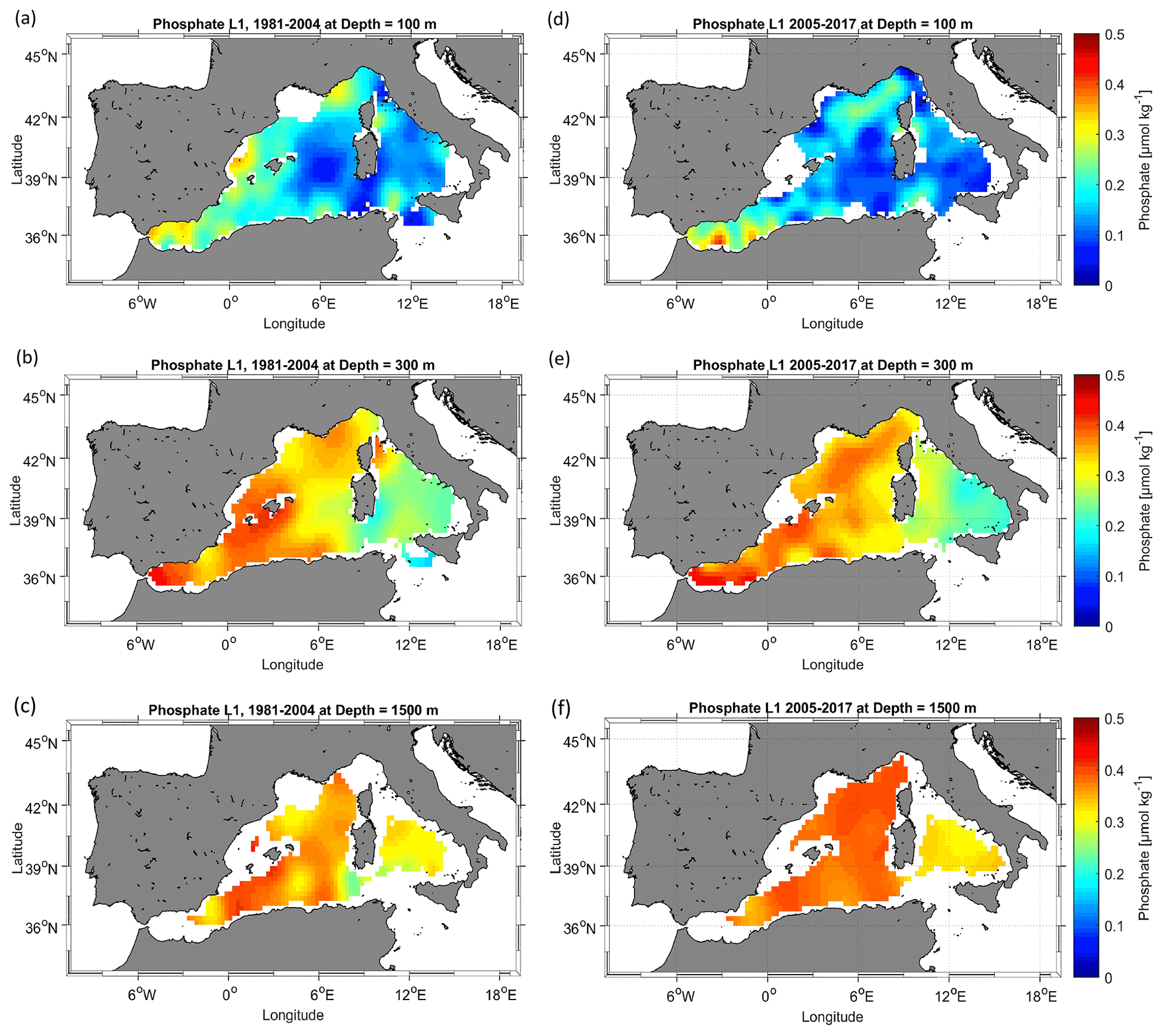
Figure 20 The same as Fig. 19 but for phosphate.

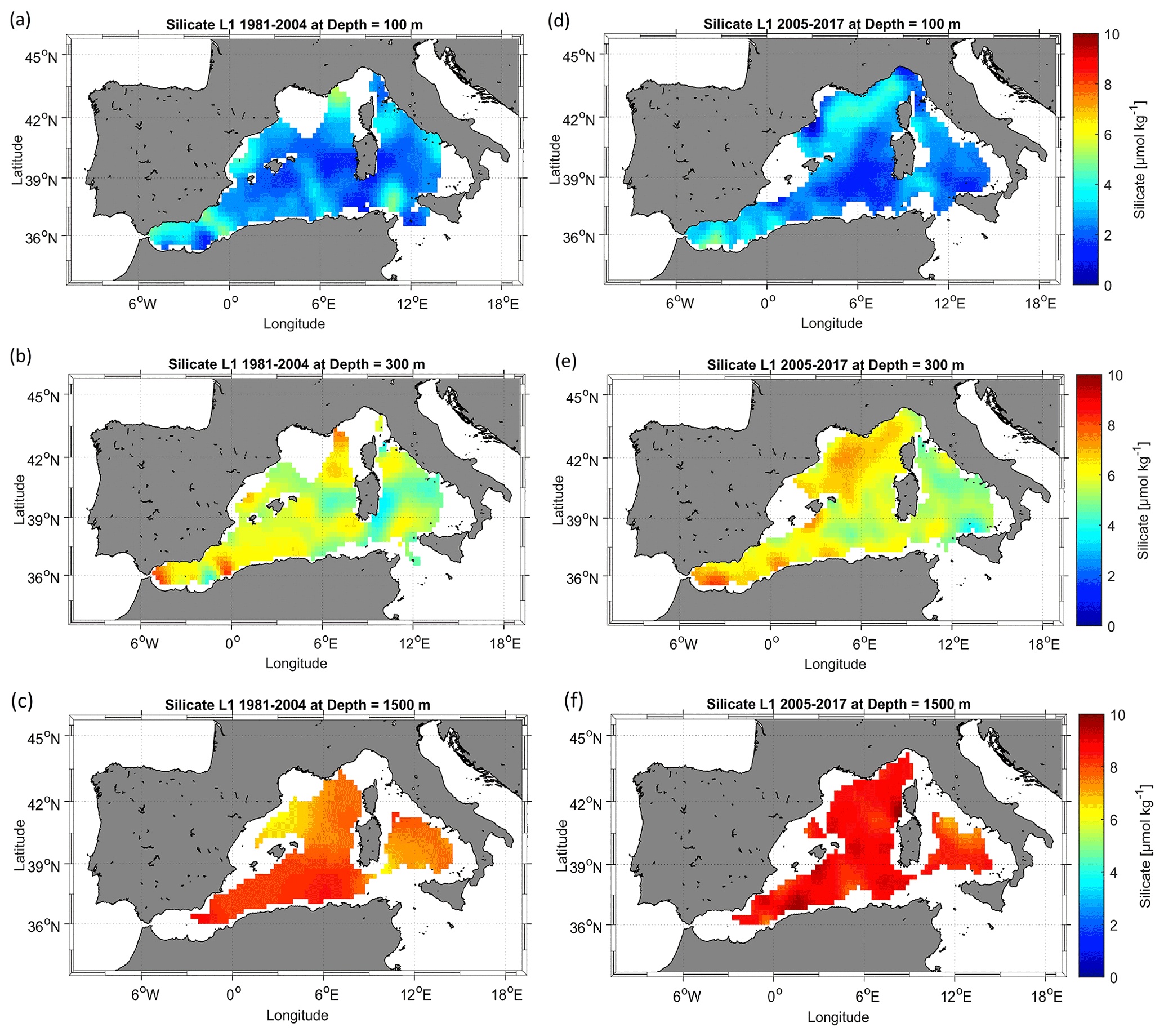
Figure 21 The same as Fig. 19 but for silicate.

We considered depth levels that represent the usual three layers: the surface (100 m; Figs. 19a and d, 20a and d, and 21a and d), intermediate (300 m; Figs. 19b and e, 20b and e, and 21b and e) and deep (1500 m; Figs. 19c and f, 20c and f, and 21c and f) layers.

The WMED surface layer is dominated by the AW coming through the Alboran Sea, a permanent area of upwelling (García-Martínez et al., 2019), where there is a continuous input of elements from the layer below to the surface (Figs. 19a, 20a and 21a). Nitrate increased after the WMT (Figs. 19d, 20d and 21d) by +0.4137 µmol kg⁻¹ (Fig. C1a). The largest difference between the two periods reached > +2 µmol kg⁻¹ in the Sardinia Channel and the Alboran Sea, which was explained by the favorable conditions for nitrogen fixation as discussed in Rahav et al. (2013), revealing also that the nitrogen fixation rate increased from east to west. Phosphate and silicate on the other hand showed a decrease at 100 m (Fig. C1a), with about −0.021 and −0.1365 µmol kg⁻¹ on average, respectively. Large changes are noticed in the southern Alboran Sea, Sardinia Channel and Balearic Sea.

The surface layer exhibits an irregular distribution since it is subjected to seasonal variability. We found an increase in all nutrients at 300 and 1500 m with a maximum identified at intermediate depths in both nitrate and phosphate, which is explained by the remineralization of organic matter along the path of the IW. The latter flows westward (from the Levantine Sea to the Atlantic Ocean). Its nutrient content increases (relatively to the conditions in the EMED) with age (Schroeder et al., 2020). It arrives at the Tyrrhenian Sea, where, in Figs. 19b, 20b and 21b (at 300 m depth, 1981–2004), we identify a nutrient-depleted intermediate layer. At this depth level, we observe a gain in the three nutrients after the WMT (Figs. 19e, 20e and 21e). On average, the difference between the two periods (pre- and post-WMT) for nitrate, phosphate and silicate is around +0.8648, +0.0068 and +0.2072 µmol kg⁻¹ (Fig. C1b), respectively.

A similar increase after the WMT in the deep layer (1500 m) is also found for nutrient concentrations (Figs. 19f, 20f and 21f) at a magnitude of +0.753 for nitrate, +0.025 for phosphate and +0.867 µmol kg⁻¹ for silicate (Fig. C1c), which highlights an increase in the downward flow of organic matter remineralization that is supplying the existing pool.

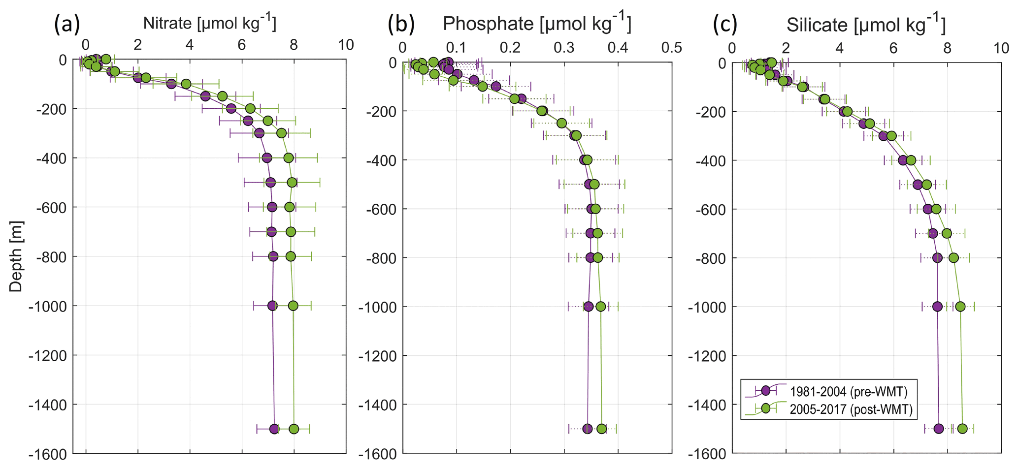
Figure 22 Climatological mean vertical profile and standard deviation of (a) nitrate, (b) phosphate and (c) silicate over the WMED before (1981–2004, in violet) and after (2005–2017, in green) the  WMT.

This increase is also illustrated in the climatological mean vertical profile of Fig. 22 of the three nutrients. Nitrate displays a notable vertical difference to the pre-WMT period below 200 m (Fig. 22a). The phosphate difference between the two time periods is larger below 400 m (Fig. 22b). Silicate is different from nitrate and phosphate. It increases progressively with depth (Fig. 22c) and demonstrates an enrichment of the DW compared to the 1981–2004 period (Fig. 21c). The maximum values are found in the deep layer due to the low remineralization rate. With the warming climate, biogenic silica tends to dissolve faster, which explains the high concentrations all over the basin, even in the Tyrrhenian Sea, after the WMT.

According to Stöven and Tanhua (2014), the impressive volume of the newly formed DW during 2004 and 2006 ventilated the old DW, decreasing its age and meaning that the WMT could have led to the lowering of the WMED deep-layer pool in terms of nutrients as was pointed out by Schroeder et al. (2010). However, we did not observe this decrease in the climatological analysis after the WMT. This might be due to the temporal variability in the deep convection intensity since a decrease was recorded in the Gulf of Lion between 2007 and 2013 (Houpert et al., 2016).

A decrease in the deep convection intensity since the WMT (Houpert et al., 2016; Li and Tanhua, 2020) could potentially lead to the reduction in the supply from the nutrient-rich DW (before the WMT) to the surface; i.e., the decrease in nutrients could have happened immediately after the WMT in spring 2005, for which Schroeder et al. (2010) reported peculiar divergence between the old WMDW and the new WMDW in nitrate and phosphate; the new WMDW was low in nutrients. Later on an intense DW formation event marked the year 2012 with strong ventilation that was recorded in the Adriatic Sea and could have affected the WMED. It was not possible to observe this change since we calculated the mean state of the basin spanning a specific period.

The spatial distribution of nutrient concentrations after the WMT (2005–2017) was quite different from the one before the WMT (1981–2004). This could also be related to the significant decline in river discharge between 1960 and 2000, which was estimated to be 20 % (Ludwig et al., 2009). The decrease is also observed in silicate fluxes since silicate increases through river discharge.

The change could be explained by the low denitrification rate for nitrate and an increase in the remineralization of organic matter. Ludwig et al. (2009) reported an increase in nitrate and phosphate fluxes that was enhanced by anthropogenic inputs, loading the deep layer with inorganic nutrients; it could also be associated with the slower ventilation of the WMED waters and a longer residence time.

5 Data availability

The climatologies of nitrate, phosphate and silicate are available as netCDF files from the data repository PANGAEA and can be accessed at https://doi.org/10.1594/PANGAEA.930447 (Belgacem et al., 2021). Ancillary information is in the readme in PANGAEA with the list of variables that are described in Table 3 of Sect. 4. The CNR_DIN_WMED_20042017 data are available from PANGAEA (https://doi.org/10.1594/PANGAEA.904172, Belagcem et al., 2019). The MOOSE-GE data are available in the SISMER database (global https://doi.org/10.18142/235, Testor et al., 2010).

6 Conclusions

In this study, we investigated spatial variability in the inorganic nutrients in the WMED and presented a climatological field reconstruction of nitrate, phosphate and silicate using an important collection dataset spanning 1981 to 2017. The new BGC-WMED product is generated on 19 vertical levels on a grid with a $\mathrm{1}/\mathrm{4}$^∘ spatial resolution.

The new product represents very well the spatial patterns of nutrient distribution because of its higher spatial and temporal data coverage compared to the existing climatological products (see Table 1); it contributes to the understanding of the spatial variability in nutrients in the WMED.

The novelty of the present work is the use of the variational analysis that takes into consideration physical and geographical boundaries, topography, and the resulting estimate of the associated error field.

Comparison with previously reported studies indicates that the BGC-WMED reproduces common features and agrees with previous records. The reference products of the WOA18 and MedBFM biogeochemical reanalysis tend to underestimate nutrient distribution in the region with respect to the new product.

The new product captures the strong east–west nutrient gradient and vertical features. The results obtained do not include seasonal or annual analysis fields. However, the aggregated dataset here does show improvements in describing the spatial distribution of inorganic nutrients in the WMED. We acknowledge that computing a climatological mean over a time period is not enough to estimate and detect the trend driven by the climate shift WMT change. However, comparing climatologies based on the two time periods, 1981–2004 (pre-WMT) and 2005–2017 (post-WMT), has already produced important results. Notable changes have been found in the nutrient distribution after the WMT at various depths.

The results support the tendency toward a relatively increasing load of inorganic nutrients to the WMED and possibly relate the change in general circulation patterns to changes in deep stratification and warming trends; however, this remains to be evidenced.

The BGC-WMED is a regional climatology that has allowed the identification of a substantial enrichment of the waters, except in the Tyrrhenian Sea where the water column is depleted in nutrients with respect to the western areas of the WMED. The climatology gave information about the spreading of inorganic nutrients inside the WMED at surface, intermediate and deep layers.

A future work will suggest a better understanding of the change in nutrients related to water masses associated with the ventilation rate, a climatological field along isopycnal surfaces instead of depths, and the correlation between potential temperature and nutrients.

Appendix A: Additional information about cruise metadata

Table A1 Summary table of the analytical techniques and instruments used for nutrient analysis.​​​​​​​

^* last access: 9 September 2019​​​​​​​

Appendix B: Additional information about quality assurance

Table B1 Summary of the quality check analysis quality assurance of the 1981–2017 climatology.

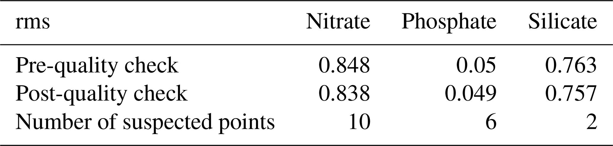
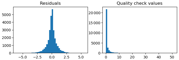
Figure B1 Overview of residual distribution and quality check values for nitrate gridded fields (1981–2017) before the quality check.

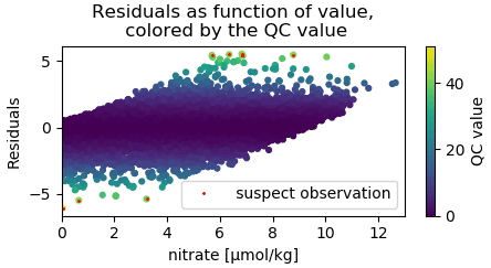
Figure B2 Scatterplot of residual as function of nitrate values (1981–2017) colored by the quality check values. The red dots are the suspect observation (points with QC values > 40).

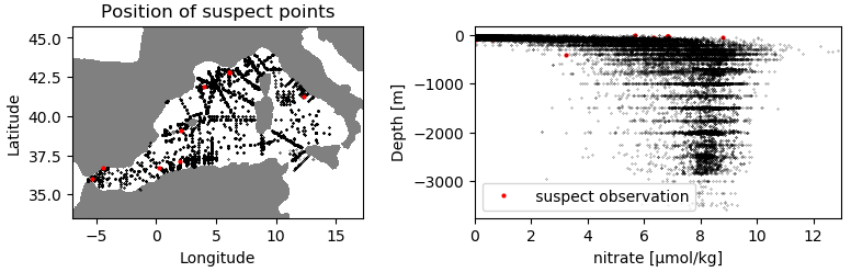
Figure B3 Position of the suspect points (nitrate climatology, 1981–2017).

Appendix C: Additional information about temporal comparison

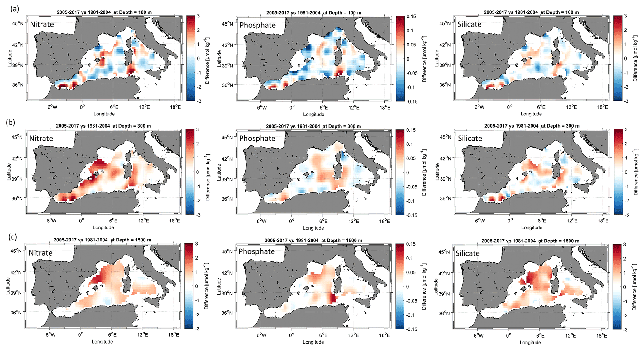
Figure C1 (a) Difference field at 100 m between the 1981–2004 climatology and the 2005–2017 climatologies; (b) difference field at 300 m; (c) difference field at 1500 m.