Estimating population and urban areas at risk of coastal hazards, 1990–2015: how data choices matter

The accurate estimation of population living in the low-elevation coastal zone (LECZ) – and at heightened risk from sea level rise – is critically important for policymakers and risk managers worldwide. This characterization of potential exposure depends on robust representations not only of coastal elevation and spatial population data but also of settlements along the urban–rural continuum. The empirical basis for LECZ estimation has improved considerably in the 13 years since it was first estimated that 10 % of the world's population – and an even greater share of the urban population – lived in the LECZ (McGranahan et al., 2007a). Those estimates were constrained in several ways, not only most notably by a single 10 m LECZ but also by a dichotomous urban–rural proxy and population from a single source. This paper updates those initial estimates with newer, improved inputs and provides a range of estimates, along with sensitivity analyses that reveal the importance of understanding the strengths and weaknesses of the underlying data. We estimate that between 750 million and nearly 1.1 billion persons globally, in 2015, live in the ≤ 10 m LECZ, with the variation depending on the elevation and population data sources used. The variations are considerably greater at more disaggregated levels, when finer elevation bands (e.g., the ≤ 5 m LECZ) or differing delineations between urban, quasi-urban and rural populations are considered. Despite these variations, there is general agreement that the LECZ is disproportionately home to urban dwellers and that the urban population in the LECZ has grown more than urban areas outside the LECZ since 1990. We describe the main results across these new elevation, population and urban-proxy data sources in order to guide future research and improvements to characterizing risk in low-elevation coastal zones (https://doi.org/10.7927/d1x1-d702, CIESIN and CIDR, 2021).

1 Introduction

Climate change threatens people around the world but particularly in locations where concentrations of people can be expected to overlap with concentrations of physical hazards resulting from climate change. Low-elevation coastal zones (LECZs) are likely to contain a disproportionate and growing share of such locations. Sea level rise and a greater prevalence of extreme weather events are correlates of climate change and heighten the risks of flooding, coastal erosion, groundwater salinization and other hazards in low-lying coastal areas (Oppenheimer et al., 2019). People are also more concentrated in coastal areas, and continued urbanization can be expected to increase this concentration, unless urban development patterns change substantially. Urbanization and related water abstraction, especially in deltas where natural subsidence is often already occurring, can also contribute to subsidence, which adds to and amplifies the hazards associated with sea level rise and extreme weather events (Nicholls et al., 2021). As such, quantifying urbanization within the LECZ is both important to monitoring the sources and pathways creating these hazards and to identifying increasing concentrations of receptors, who will bear a growing share of burden. The hazards of concern not only threaten human life and wellbeing directly but also have adverse consequences for the homes, businesses and infrastructures characteristic of built-up areas, as well as local ecosystems and the services they provide. The principal purpose of delineating a low-elevation coastal zone (LECZ) is to identify the broad areas in which there are likely to be sub-populations at a heightened and rising risk of exposure to selected hazards being exacerbated by climate change. The hazards of particular concern here are those arising from sea level rise and more extreme weather events and being aggravated by land subsidence where that is occurring.

A foundational study of settlement in the LECZ globally (McGranahan et al., 2007a) found that in the year 2000, coastally contiguous areas of less than 10 m in elevation contained an estimated 10 % of the world's population and 13 % of its urban population. That study also contained case studies of China and Bangladesh, suggesting that from 1990–2000, populations in these countries' LECZs were growing faster than outside the LECZ, with urban LECZ populations growing fastest of all. Since that study, a number of new tools and data sets have been developed, allowing for more refined estimates of land areas, built-up areas and populations in LECZs and their changing urban–rural compositions over a number of years (1990–2015).

Accurate estimates of populations living in the LECZ depend on robust representations of coastal elevations (Gesch, 2018; Hinkel et al., 2014; Lichter et al., 2010; Hooijer and Vernimmen, 2021) and population at a fine resolution (Mondal and Tatem, 2012; Leyk et al., 2019a). Estimates of urban population and land in the LECZ require additional data on the spatial extent and density of urban areas, ideally encompassing a full urban–rural continuum of settlements (Dijkstra et al., 2020; OECD and European Commission, 2020). While the empirical basis for such estimates has improved considerably (cf. the excellent review in McMichael et al., 2020) since the first analysis (McGranahan et al., 2007a), there has also been a proliferation of new internationally available data sources containing a wide range of estimates of the population in LECZs. For example, a recent study finds that “New elevation data triple estimates of global vulnerability to sea level rise and coastal flooding” (Kulp and Strauss, 2019). To improve decision-making there needs to be a better understanding of the strengths and limitations of each data set, the applications each is best suited for and why estimates vary so widely. This study fills that gap by constructing new estimates of population and land area found along the urban–rural continuum within the LECZ, based on four elevation data sources, four population data sources and four urban-proxy data sources, each with their own strengths and weaknesses, all designed to be internationally comparable and substantially improved in the past decade (Leyk et al., 2019a; Gesch, 2018).

Improvements in the spatial resolution of these data sets also allows for a more fine-grained analysis of potential exposure: within the ≤ 10 m LECZ and along an urban–rural continuum. Using four elevation sources, we first constructed the LECZs: ≤ 5 m above sea level, 5–10 m above sea level (which can be added together to form a ≤ 10 m LECZ), and a category of higher coastal areas and non-coastal areas of any elevation. We then estimated the population of these LECZs, disaggregated by settlement type, based on an array of population sources and urban-proxy data sets. The four elevation data sets obtain their estimates through a variety of different sensors, which in one case (CoastalDEM; digital elevation model) is combined with statistical modeling. The four population data sets use different approaches to mapping and disaggregating population, and the four data sets representing the urban–rural continuum use a variety of different underlying data sources, such as satellite imagery of built-up areas or nighttime lights and different modeling approaches (some with population criteria, others without) to categorize the level of urbanization of settlements. Defining an urban–rural continuum, largely in contrast to defining population, requires researchers to make decisions that reflect the best available knowledge and expert judgments but are at some level necessarily arbitrary or may be more suitable for some research questions than others.

The primary focus of this paper is on methodology and includes a sensitivity analysis in order to compare the many sources of population, urban-area delineation and digital elevation models used to construct the LECZs and estimate at-risk populations. The sensitivity analysis reveals similarities and differences in each of the data sources that we considered for population, urban proxy and elevation as well as indicates how the results would change if the measures along an urban–rural continuum were defined with a different indicator (such as nighttime lights rather than a built-up area) or if the thresholds or boundaries of the definitions were adjusted.

We begin in the section on “Data and methods” with summaries of input sources and continue with a detailed description of how the LECZs were constructed and how populations and land areas were tabulated. This is followed by a “Results” section which includes a series of zonal summaries of gridded population data categorized by LECZ and along an urban–rural continuum for three time points (1990, 2000 and 2015) and the sensitivity analysis. Finally, there is a discussion of fitness for use along with conclusions and future research needs. Accompanying this paper are tabular data on country-level summaries (http://ciesin.columbia.edu/data/lecz-urban-rural-population-land-area-estimates-v3/, last access: 1 November 2021) as well as spatial data, where redistribution is permissible, and a Python notebook which provides an algorithm to produce LECZs from elevation and coastline data (CIESIN and CIDR, 2021).

2 Data and methods

The basic method used here to quantify potential exposure to sea level rise is based on fairly straightforward spatial summaries (zonal statistics) but depends on substantial improvements to and suitable conditioning of underlying data sets, which we describe in detail below. There have been many advances in earth observation, population censuses and scientific computing capacity since the original LECZ Urban-Rural Population Estimates, v1 (1990, 1995, 2000) data set (McGranahan et al., 2007b) was constructed. In this section, we provide an overview of the various input data sets, including a discussion of the uncertainties. Such uncertainties may have considerable impacts on the ultimate estimates of persons, particularly when stratified along an urban–rural continuum in the LECZ, and must therefore be carefully understood (Gesch, 2018; Hawker et al., 2019; Uuemaa et al., 2020; Mondal and Tatem, 2012; Lichter et al., 2010; Leyk et al., 2019b). Since it has been shown that accuracy of the digital elevation models (DEMs) – upon which the LECZs are based – is highly sensitive to local conditions, including land cover, it is therefore sensible to evaluate a variety of DEMs that can be used to estimate population and land area in the LECZ. In this section, we describe the data strengths and limitations, along with the conditioning, transformations and processing required to generate LECZs and accompanying population and land area estimates along an urban–rural continuum. At the end of each type of data, we choose a “core data set” to form the basis of comparison with all others and to simplify the presentation of results. (Estimates available on all combinations of the data sets are available in the data set.) Rationales for our selection of these core data sets are given.

2.1 Data on elevation

For elevation data to construct the LECZ, we considered the sources as described in Table 1 and shown in Fig. 1. These data are all freely available at 3 arcsec horizontal resolution or higher, but some have restrictions on usage and redistribution of derived data products. There is general agreement that the newer data products have made substantial improvements in vertical accuracy since the early releases of the Shuttle Radar Topography Mission (SRTM) data (Gesch, 2018; Hawker et al., 2019; Uuemaa et al., 2020). We selected four data sets for use here based largely on recent studies, such as that by Gesch (2018), which finds that only some of the global DEMs are suitable for delineating the LECZ ≤ 10 m elevation at or above the 68 % confidence level (including TerraSAR-X add-on for Digital Elevation Measurements, TanDEM-X; CoastalDEM; NASADEM; ALOS World 3D – 30 m, AW3D30; and Multi-Error-Removed Improved-Terrain DEM, MERIT DEM), whereas other data sets (such as SRTM) are not. (SRTM nonetheless is included here in order to compare to previous work.) Despite compelling interests from the policy arena, it should be noted that the implication of Gesch's (2018) study is that delineating LECZs in finer increments than 10 m is subject to great uncertainty. (Hooijer and Vernimmen's (2021) recent study uses a digital terrain model to generate lidar data rather than those primarily used here, in order to estimate land area and population up to 2 m above mean sea level, but use of this welcomed addition to the literature will be deferred to future research.)

Major improvements of these data notwithstanding, we discuss below considerations specific to the coastal zone (such as detection of and correction for mangrove forests) and to urban areas (where man-made structures may bias measurement). The 2019 study by Hawker et al. (2019) identifies the types of land cover that each of these data sets best detects or is prone to misinterpret (see the graphical abstract and Table 4 in Hawker et al., 2019). While urban environments are evaluated in these recent studies, urban is just another land cover class. To our knowledge, no targeted or multi-criteria evaluation of these global elevation data sets in the urban setting has been made (but see related analysis of the built environment in cities, which leverages TanDEM-X; Esch et al., 2020). Furthermore, case studies reveal that the data sets which perform best globally, on average, may not necessarily be the most accurate in a given location or under particular geographic conditions (Minderhoud et al., 2018, 2019). Notably these global DEMs tend to do a comparably poor job of capturing low-lying elevation in small island states (Taupo and Noy, 2016; Taupo et al., 2018; Yamano et al., 2007; Lewis, 1989). Once again, there are important policy implications here.

The scientific community of modelers that produces the many relevant data sets and models to predict sea levels, tides, storm surges and other coastal flooding is large, growing and vibrant. Future LECZ estimates stand to be substantially improved by their current efforts. In this work, we have used global elevation data sets to construct LECZs using a simple but inclusive approach. Global hydrodynamics-based models could potentially provide a better basis for identifying some of the relevant hazards, including most notably those caused by flooding. However, at the time of this writing the results of global models that account for the fuller and complex set of factors at and connected to the seacoast are not available. Local studies (Schumann and Bates, 2018; Orton et al., 2020; Khan et al., 2020) suggest clearly that the hydrodynamics of the coastal zone are complex and nuanced, perhaps even more so in urban areas where impervious surface, underground infrastructure (sewage and subway systems) and other modifications to the landscape (including accumulations of uncollected solid waste) may impact inland flows and drainage. New work on coastal storm surges and tidal heights (Muis et al., 2020; Arns et al., 2020) and empirical flood events (Tellman et al., 2021) make new avenues of research possible in the coming years, but currently hydrodynamic modeling has been restricted to certain locations or events.

Table 1 Elevation data sets used in the construction of the low-elevation coastal zones (LECZs).

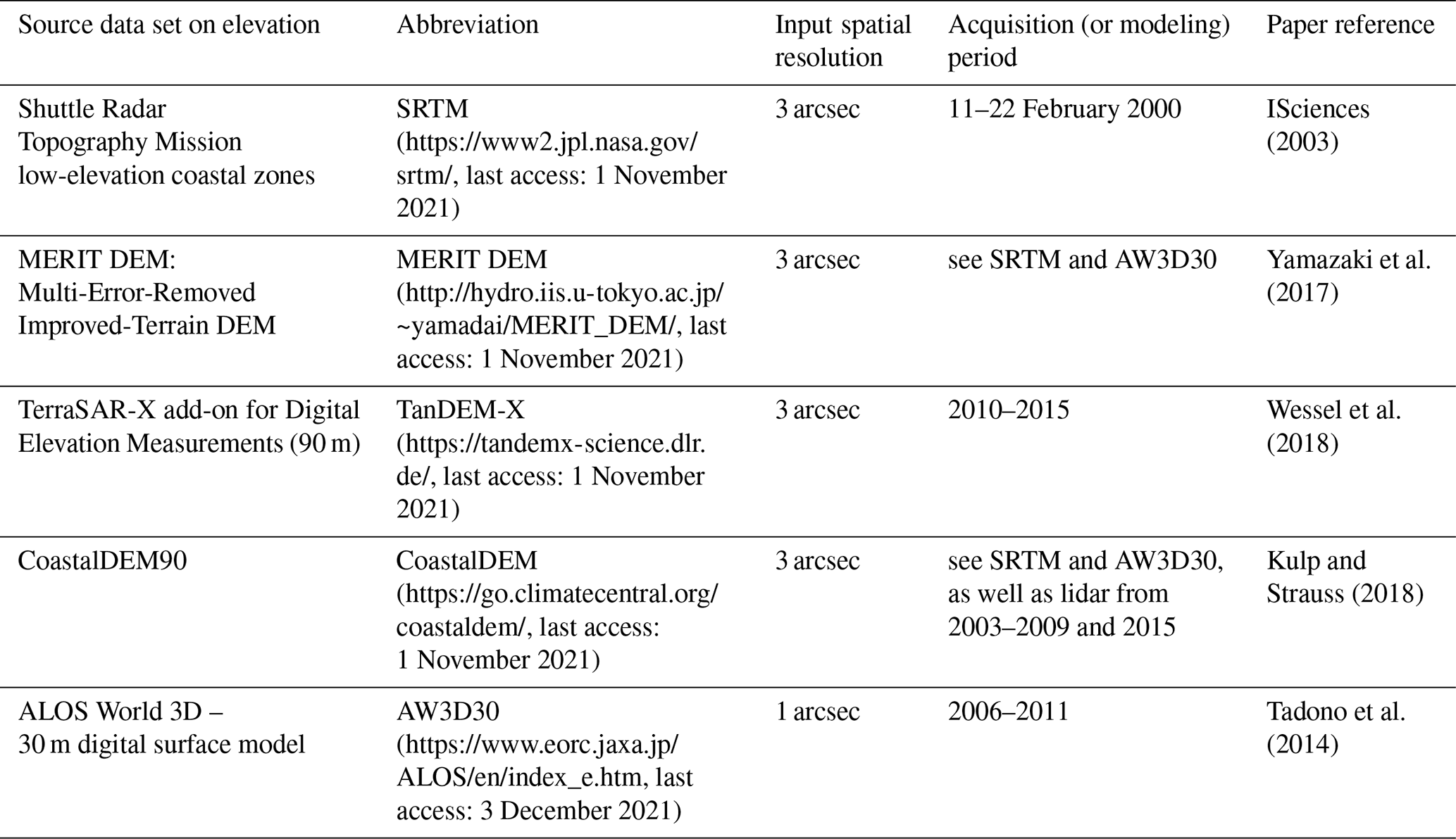
NB: ALOS 30 m global DEM is used as a supplement in CoastalDEM90 at latitudes north of 60^∘ N and south of 56^∘ S. It is also used as an input data set in the construction of MERIT DEM.

2.1.1 SRTM

The NASA Shuttle Radar Topography Mission (SRTM) set the standard for characterizing global elevations, but the SRTM data products, now nearly 20 years old, have been widely understood to have limitations in some critical areas. There is, for instance, a high root mean square error (RMSE) in the elevation estimates of mangrove forests (Gesch, 2018). These vertical errors (termed tree height bias) are particularly problematic in some low-lying vegetated areas (such as in populous southeastern Bangladesh). A coastally contiguous derivation of SRTM was produced in 2003 by ISciences, Ltd., and it was these data which were used in the first LECZ study (McGranahan et al., 2007a) and the NASA SEDAC (Socioeconomic Data and Applications Center) update (CIESIN, 2013). We include the same data here exclusively for the purpose of comparison with the original study.

2.1.2 MERIT DEM

The Multi-Error-Removed Improved-Terrain DEM (MERIT DEM), “separated absolute bias, stripe noise, speckle noise and tree height bias using multiple satellite data sets and filtering techniques” to improve on the SRTM baseline (Yamazaki et al., 2017). The Japanese Aerospace Exploration Agency (JAXA) produces the ALOS Global Digital Surface Model (DSM) “ALOS World 3D – 30 m” (AW3D30), which along with SRTM3 v2.1 was used as primary data in the construction of MERIT DEM. In the land cover classes of short vegetation and forested areas, MERIT DEM performs well when compared to locally available lidar data (Hawker et al., 2019). Compared to TanDEM-X, which Hawker et al. (2019) find to be of comparable overall accuracy, MERIT DEM has a marginally higher margin of error (ME) (1.09 m) but lower mean absolute error (MAE) (1.69 m) and RMSE (2.32 m). If the RMSE metric is the only metric considered, MERIT DEM is the most accurate global DEM across land cover types. Uuemaa et al. (2020) found that MERIT DEM performed well in accuracy tests, despite having a coarser resolution than SRTM. Despite these many improvements, Gesch (2018) notes that MERIT DEM has an RMSE of about 3 m globally, which has implications for producing LECZs in finer increments below 10 m.

2.1.3 TanDEM-X 90 m

The TerraSAR-X add-on for Digital Elevation Measurements (TanDEM-X) departs from an SRTM baseline and provides a new SAR-interferometry-based (synthetic-aperture radar) estimate of elevations globally (Wessel et al., 2018; Zink, 2014). TanDEM-X has been shown to be the most accurate global DEM in some land cover categories (bare, shrubland, sparse vegetation and urban) (Hawker et al., 2019), and at the 95 % confidence level, Gesch (2018) finds that only TanDEM-X is suitable for delineating the LECZ below 10 m. Wessel et al. (2018) found TanDEM-X to have biases in areas of rugged terrain, where there is heterogeneity in the landscape/land cover and elevation, and additional analyses have revealed that while TanDEM-X is highly accurate in flat to slightly undulating terrains, it tends to overestimate elevation when used in areas characterized by more sharply uneven terrain (Bhardwaj, 2019). Higher-resolution versions of TanDEM-X (0.4 and 1 arcsec) are available through proposal and a service fee for scientific use but were not utilized in this study. While no study has closely examined the vertical accuracy of these DEMs globally for urban areas, an analysis by Hawker et al. (2019) does suggest that TanDEM-X may be well-suited to capturing elevation in core urban areas where high-rise buildings are common (for specific cities, some analysts have used TanDEM-X for urban elevation mapping – Rossi and Gernhardt, 2013 – to construct urban extents; Esch et al., 2012, 2013). However, TanDEM-X's restrictive licensing limits dissemination and replicability, making it less useful for many purposes.

2.1.4 CoastalDEM90 and ALOS World 3D

CoastalDEM utilizes neural networks with an array of spatial covariates to improve on SRTM (see Fig. 1 in Kulp and Strauss, 2018). CoastalDEM90 is made available for research free of charge, and a higher-resolution (1 arcsec) version of CoastalDEM is available with a licensing fee. AW3D30 was used as supplemental data for CoastalDEM in latitudes north of 60^∘ N and south of 56^∘ S, as was done by the data authors. CoastalDEM is produced from a 23-dimensional vertical error regression analysis using variables including neighborhood elevation values, pop density, land slope and local SRTM deviations from ICESat (Ice, Cloud and land Elevation Satellite) altitude observations, and vegetation cover indices. Importantly, since one of the covariates is population density from LandScan 2010 (resampled to 1 arcsec), estimation of population exposure in the LECZ is complicated, since population itself was used to determine elevation values. Studies by the data producers show that in the Caribbean basin, the CoastalDEM data provide greater vertical accuracy than other data sets, including the SRTM data and AW3D30 data set which both overestimate by more than 2 m on average (Kulp and Strauss, 2018). However, Gesch (2018) notes that globally CoastalDEM, like MERIT DEM, has an RMSE of about 3 m, implying a need for caution when using it to delineate LECZs in increments finer than 10 m.

2.1.5 Core data choice – elevation

Hawker et al. (2019) evaluated the accuracy of global DEMs by land cover type and found that both TanDEM-X and MERIT DEM outperform SRTM across all categories and that MERIT DEM achieves greater accuracy than TanDEM-X in short-vegetation and forested land cover classes. CoastalDEM performs well in the Caribbean basin (Strauss and Kulp, 2018) but globally has a similar RMSE to MERIT DEM. According to Gesch (2018), TanDEM-X, with an RMSE of 1.69 m, can be used to delineate the ≤ 10 m LECZ with the greatest confidence, but MERIT DEM and CoastalDEM, which have RMSEs of ∼ 3 m, can be used, albeit with somewhat less confidence (see Table 5 in Gesch, 2018). However, as is shown below, the precision of TanDEM-X results in a highly varied landscape, with raised roadways clearly identified at higher elevations than surrounding land. This results in wide areas of TanDEM-X losing their direct connectivity to the coast according to image segmentation (region grouping) methods and therefore removes them from the LECZ, which requires coastal contiguity. Additional research on the presence of natural (wetlands and floodplains) and man-made (raised berms and buildings) barriers as well as connections (sewer systems, stormwater management systems/culverts, estuaries and other water channels) is needed in order to improve the TanDEM-X-based LECZ.

We have selected MERIT DEM as the core elevation data set. This is because of the complications with identifying coastal connections in TanDEM-X and since MERIT DEM is the only elevation data set considered which is both accurate (Gesch, 2018; Hawker et al., 2019; Uuemaa et al., 2020) and has wide dissemination rights (open for use both non-commercially and commercially so that any data we create from it can be widely and openly distributed as well, both in spatial and tabular formats; Yamazaki et al., 2017).

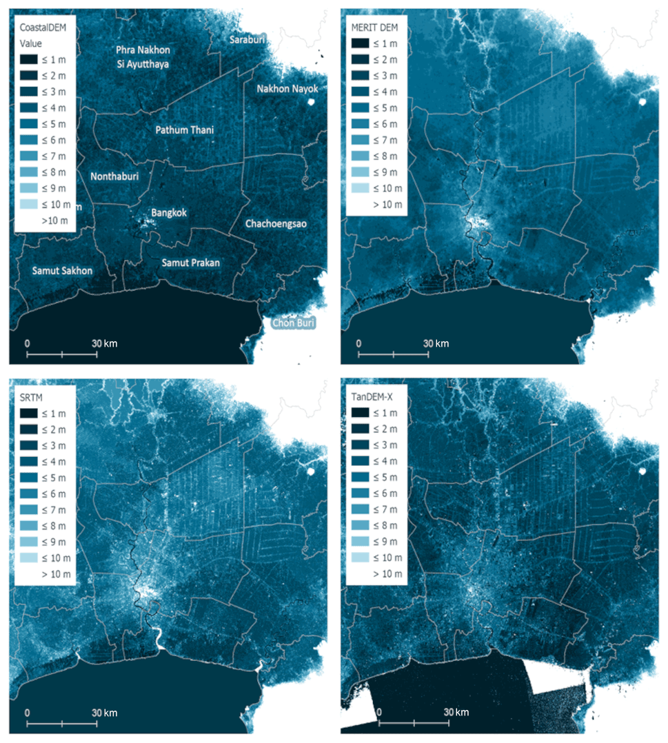
Figure 1 Elevation source data for constructing low-elevation coastal zones (LECZs), Bangkok and surrounding areas, Thailand. Note that the darkest blue indicates ocean, and gray boundaries indicate first-order administrative boundaries.

2.2 Data on population

For population data, we compared several data sets from the leading producers of global population data, listed in Table 2 and visualized for Bangkok in Fig. 2. Mondal and Tatem (2012), as well as Lichter et al. (2010), compared several gridded population data sets and recommended that studies utilizing a particular data set should acknowledge how the inherent uncertainties of the underlying input data and methods are likely to impact conclusions. A recent and thorough review by Leyk et al. (2019a) discussed the nature and source of these uncertainties at great length. Characteristics such as the relative resolution of underlying input vector data sets, the selection and relative accuracy of spatial covariates for dasymetric maps, and the currency of population estimates all have major impacts on grid-level population counts. For a full description of each of these, including strengths and weaknesses, please see Leyk et al. (2019a) and Table 2 for the selection of data sets we use herein.

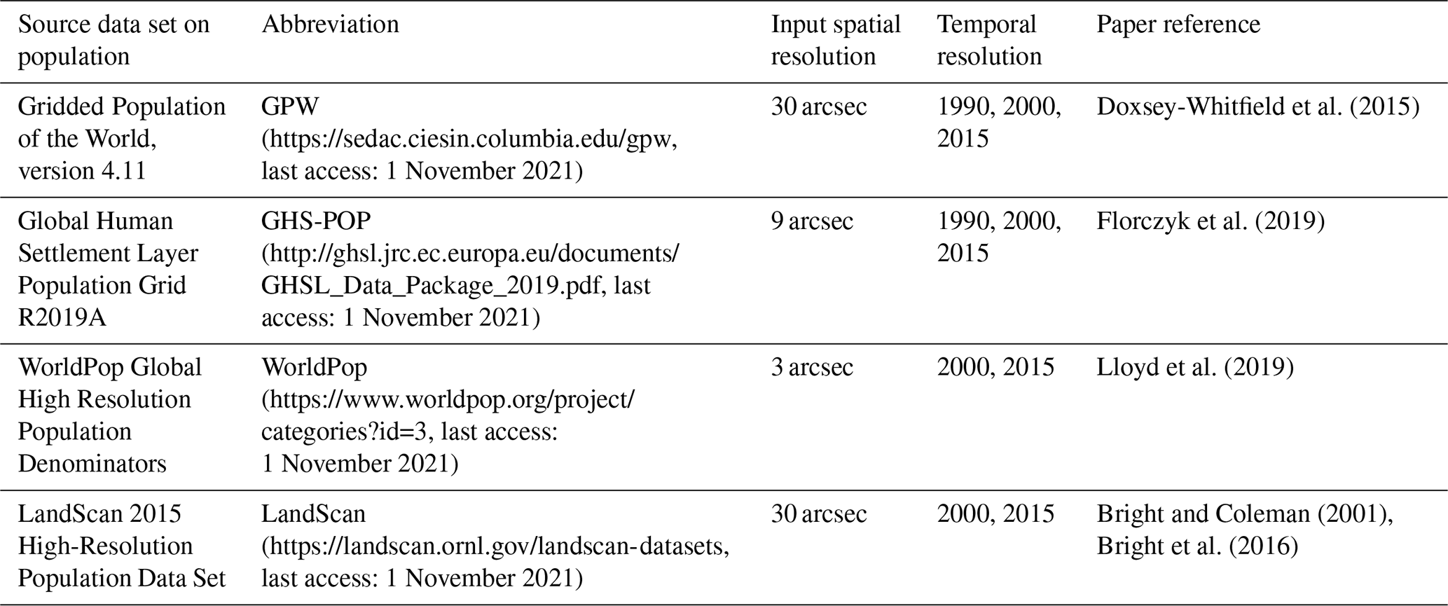
Table 2 Population data sets used to estimate persons living in the low-elevation coastal zones (LECZs).

2.2.1 GPW

Gridded Population of the World, version 4.11 (GPW) is a minimally modeled 30 arcsec horizontal-resolution data set which uses source data from the 2010 round of international censuses. Because GPW uses a uniform allocation across space to distribute census-based populations across the smallest areas for which population estimates were made available, the accuracy of its estimates at a pixel level is very closely linked to the relative resolution of input vector data (MacManus and Kugler, 2013). The layer “Mean Administrative Unit Area” (CIESIN, 2018a) in the GPW data collection provides an indicator of the relative size of input geographies (administrative areas refer here loosely to the units in which census data are reported and may include enumeration areas, which typically are statistical rather than administrative, as well as truly administrative areas used for reporting) and is used here along with the GPW UN-WPP-adjusted population count data set (CIESIN, 2018d), which adjusts census-reported national totals to estimates from the United Nations World Population Prospects (Doxsey-Whitfield et al., 2015; United Nations, 2018). When overlaying a population grid with irregularly shaped and variably sized zones (such as a narrow LECZ in some locations), a uniform allocation method of coarse underlying data will sometimes lead to misestimation (Mondal and Tatem, 2012; Balk et al., 2009). However, an important advantage of the uniform allocation approach is that these data do not include additional spatial layers which could themselves be the source of errors and uncertainties.

2.2.2 GHS-POP

The Global Human Settlement Population Grid R2019A (GHS-POP) is derived from GPW inputs and the Global Human Settlement Layer (GHSL) built-up data set (GHS-BUILT (Pesaresi et al., 2016), also discussed below) to improve the horizontal resolution and positional accuracy of free and open population data (Freire et al., 2016). A distinguishing characteristic of GHS-POP is the use of the GHS-BUILT time series, which was derived from satellite observations from the LandSat program's long history of earth observations. GHS-POP data use a dasymetric mapping approach at a 9 arcsec horizontal resolution to reallocate GPW census inputs based on the percentage built-up, as defined by GHS-BUILT (Freire et al., 2016). In this approach, population from large, sparsely populated administrative units is moved to the detected built-up areas rather than being assumed to be evenly distributed throughout the entire polygon: reallocation of population occurs in proportion to the distribution of the built-up area (within a given cell); otherwise areal weighting is applied (see Fig. 2 in Freire et al., 2016). Because GHS-POP relies on GHS-BUILT, for which detection in sparse and rural areas is lacking (Leyk et al., 2018), it may tend to over-concentrate population into built-up areas, overestimating the number of urban residents (depending on how urban areas themselves are delineated). GHS-POP has been shown in recent studies to produce the most accurate pixel-level population estimates when compared to local data for some locations, especially in urban areas (Archila Bustos et al., 2020; Calka and Bielecka, 2020).

2.2.3 WorldPop

WorldPop Global High Resolution Population Denominators (WorldPop) also use census-based population inputs from GPW to produce estimates for 2000 and 2015 (it does not include 1990). Its disaggregation approach uses country-specific machine-learning-based (ML) dasymetric models which employ random forest classifications to disaggregate population on the basis of a variety of spatial covariate layers such as slope, impervious surface, nighttime lights and others (Lloyd et al., 2019; Gaughan et al., 2015). WorldPop produces population estimates at a 3 arcsec horizontal resolution, which is the same resolution as the input elevation data. Importantly, the covariate data used to delineate WorldPop estimates include elevation as one of the weighting factors and some time-varying data sets (or those modeled to be time-varying; GHSL, the Global Urban Footprint (Esch et al., 2017), and ESA land cover). WorldPop has been shown to produce accurate disaggregations in many locations (see for example, Bai et al., 2018; Chen et al., 2020; Mohanty and Simonovic, 2021) and is widely used particularly in health applications. Like GPW, WorldPop is highly transparent in the methods and underlying inputs used in its creation.

2.2.4 LandScan

Oak Ridge National Laboratory's LandScan data set uses input population data from a variety of sources (including censuses, surveys, work and school registers, and other sources) and an ML-based dasymetric model (using a wide variety of covariates, including elevation and slope) to produce annual population estimates for 2000 and 2015 (it does not include 1990). It deviates from the other population data sets in that it aims to measure ambient population – that is, population distribution averaged over a 24 h period, rather than census de jure measures linked to usual residence. LandScan Global is a 30 arcsec population surface which is not directly comparable year over year, since methodologies are updated with each release (Bright and Coleman, 2001; Bright et al., 2016; Rose and Bright, 2014; Mesev, 2003). Thus LandScan is not suitable for use as a time series. The ML model used by LandScan is proprietary, so the efficacy of covariate sources cannot be evaluated, and LandScan is not free and publicly available for non-commercial and commercial use. Nevertheless, LandScan is a spatial population data set that is often used in policymaking (Leyk et al., 2019a) and has produced accurate disaggregations in many locations. For applications requiring ambient rather than de jure population estimates, LandScan is suitable.

2.2.5 Core data choice – population

Unlike physical data (elevation), the evaluation of the accuracy of gridded population data is complicated by the unavailability of baseline population estimates. Estimates from census and survey sources are static, and human mobility makes it difficult to validate those sources. Leyk et al. (2019a) discuss the strengths and weaknesses of global population data sets in great detail and help data users select the best data for their specific use. For our analysis, being able to construct estimates of population in the LECZ for a 25-year interval (from 1990–2015) was important in order to evaluate population change in different settlement types. In this study, we chose GHS-POP as our core population data set because it does not use elevation to reallocate population (as do LandScan and WorldPop) and represents the longest time series (back to 1990) in that it uses built-up data for each of its target years to allocate population (rather than interpolating or extrapolating estimates of population based only on growth rates, as in GPW) and was acceptable in other regards as mentioned above.

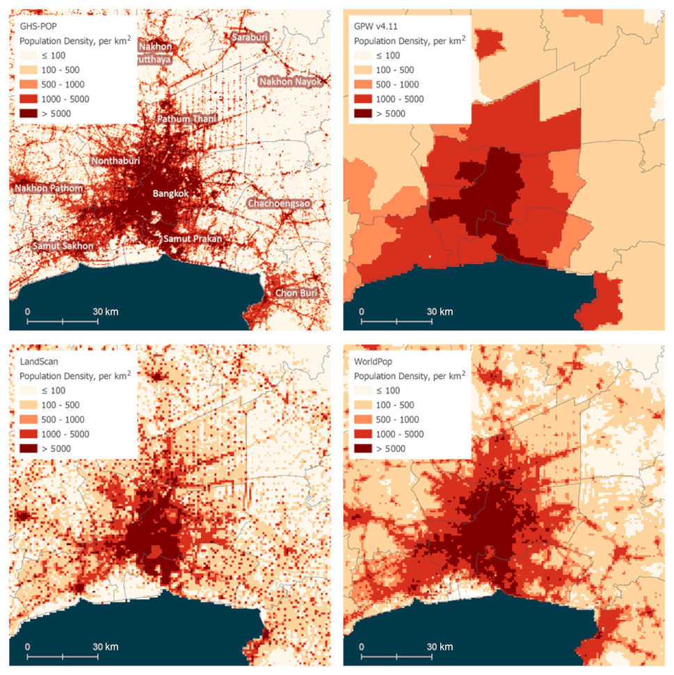
Figure 2 Population source data, Bangkok and surrounding areas, Thailand, 2015. Note that the dark blue indicates ocean, and gray boundaries indicate first-order administrative boundaries. (These images show the processed 9 arcsec data rather than the higher-resolution inputs, given that the resolution differences are hard to detect in this visualization.)

2.3 Data on urban proxy

There is no authoritative source of data to delineate urban areas in an internationally comparable manner. Indeed, national statistical agencies and different disciplines have different ways to measure urbanization (Buettner, 2015; Uchiyama and Mori, 2017). Yet since the Global Rural-Urban Mapping Project (Balk, 2009; CIESIN et al., 2021) – the first-ever global spatial rendering of urban areas and the data set used in McGranahan et al. (2007a) – as well as regarding the above advances in elevation data and population models, there have been many advancements in data, models and methods which have led to many new data sets that aim to capture settlements across the urban–rural continuum. All of these various new efforts to capture urban areas use proxy data sets – such as nighttime lights (dLIGHT, Defense Meteorological Satellite Program Change in Lights, and GRUMP, Global Rural-Urban Mapping Project) or built-up area (GHS-BUILT and GHS-SMOD, Settlement Model) – that measure conceptually different dimensions of urban classification. The data sets selected for this study are listed in Table 3. Two of the data sets we consider represent physical processes whose spatial concentration is closely related to urban settlement (dLIGHT and GHS-BUILT), while two are more heavily modeled with the goal of urban classification (GRUMP and GHS-SMOD). All of the new underlying inputs (not including GRUMP) can be expressed as continuous data, which is important for representing a fuller urban–rural continuum (Dorélien et al., 2013); here we classify the urban-proxy inputs into three large classes, described in Table 4.

Table 3 Urban-proxy data sets used to estimate persons living in the low-elevation coastal zones (LECZs).

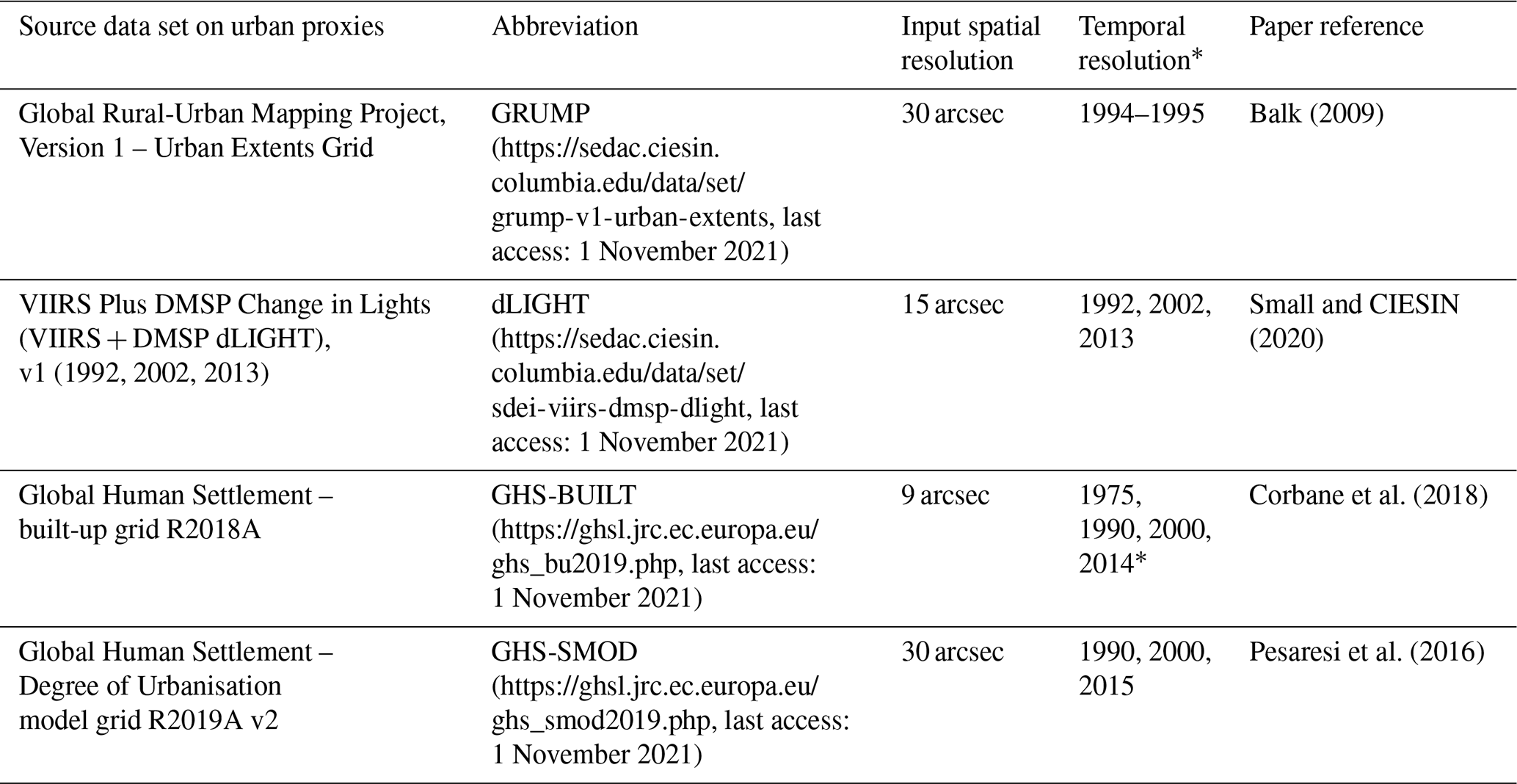
^* The temporal resolution represents acquisition years of the underlying satellite data, for GRUMP, dLIGHT and GHS-BUILT. GHS-BUILT creates “epochs”, that is, the period by which observation(s) was (were) made; in contrast, VIIRS (Visible Infrared Imaging Suite) and the nighttime lights on which GRUMP was based represent observations from a more narrow temporal range (such as 1 year). The temporal resolution of GHS-SMOD, being based on GPW and GHS-BUILT, indicates the specified target output year of the variables in question.

2.3.1 GRUMP

The Global Rural-Urban Mapping Project (GRUMP) Urban Extents Grid v1 was the first gridded global data product to delineate urban areas (CIESIN et al., 2021). This was accomplished through the use of observations of stable-city (nighttime) lights from the Defense Meteorological Satellite Program Operational Line Scanner (DMSP-OLS) circa 1995 (Elvidge et al., 1999; Small et al., 2005) and confirmed by the presence of a named settlement above a certain population size (5000 persons, where the data collection permitted). To address gaps in DMSP-OLS, these data were supplemented by “alternate sources (e.g. Tactical Pilotage Charts), or approximated by circles whose sizes were given by population–area relationships calibrated (through a regression analysis) on existing data” (Balk, 2009). GRUMP is distributed at a 30 arcsec horizontal resolution. While GRUMP has been widely used, because its urban footprint is based on the stable-city lights known for their blooming quality (Small et al., 2005), it is well known to be an inclusive measure of urban extents. Furthermore, the spatial extent of the urban area represents a simple dichotomy: urban or rural. For this reason, GRUMP (like the original SRTM-based LECZ) is only included here for the purpose of comparison with the original study.

2.3.2 dLIGHT

Because nighttime lights have been shown to be a good proxy for economic activity (Henderson et al., 2012; Donaldson and Storeygard, 2016; Ghosh et al., 2009) and because the spatial concentration of economic activity is associated with urban location, nighttime light data products continue to be a valuable data source as an urban proxy (Hu et al., 2020). The VIIRS Plus DMSP Change in Lights, v1 (dLIGHT) data set depicts the relative luminosity in stable light areas (as determined by VIIRS annual composites for the year 2015) for the years 1992, 2002 and 2013, respectively (Small and CIESIN, 2020). The dLIGHT data set combines nighttime light imagery from DMSP-OLS with a composite of stable nighttime light from Suomi National Polar-orbiting Partnership (NPP) Visible Infrared Imaging Suite (VIIRS) Day/Night Band in a 15 arcsec horizontal resolution grid. While dLIGHT makes great improvements in resolution and accuracy over DMSP-OLS, it represents relative changes in brightness of the DMSP-OLS sensor and is constrained to lit areas based on the 2015 VIIRS data (Small et al., 2018a; Small, 2020). Like some of the data sets used here, dLIGHT is a new data product and has not been used extensively with other data sets indicating the spatial extents (and change thereof) of urban areas. While there has been continued improvement to reduce gas flares from the underlying data products, because gas flares are not expected to be associated with urban areas (Elvidge et al., 2009), it is also understood that not all economic or human activity is accompanied by light sources, particularly in poor economies or in particular land covers (such as deserts) (Stokes and Seto, 2019).

2.3.3 GHS-BUILT

Another approach to urban representation comes from a land-use perspective. Early work in this area classified pixels from moderate-resolution satellite data products detecting vegetation (e.g., NDVI, normalized difference vegetation index) that were typically heterogeneous and residual and thus did not represent specific land-use classes found outside urban localities (Potere et al., 2009; Schneider et al., 2010): in other words, this approach did not directly detect structures or features typically concentrated spatially in urban areas (buildings, roads, etc). Developments in ML approaches and related modeling have led to a new class of derived products that explicitly classify built features commonly concentrated in urban settings. Recent global-scale efforts include NASA SEDAC's Global Man-made Impervious Surface (GMIS), the European Commission's Joint Research Centre's (JRC) GHSL and the German Aerospace Center's World Settlement Footprint (WSF) projects (Esch et al., 2018; Marconcini et al., 2020). Here we use two products from the GHSL suite. GHS-BUILT represents estimations of built-up presence as derived from LandSat image collections. Built-up estimates are provided for the epochs 1975, 1990, 2000 and 2014 (Florczyk et al., 2019). At its core are more than 40 000 LandSat scenes which have been processed in a consistent manner across countries and over time using advanced machine learning algorithms (Pesaresi et al., 2016). The 1 arcsec data are binary, indicating either the presence or absence of a built structure and are aggregated to 3 arcsec to represent the fraction of built-up land in each pixel. This data set has been cross-validated or analyzed with census-designated classes of urbanization in the recent studies of the US (Balk et al., 2018; Leyk et al., 2018) and generally confirmed the accuracy of the GHSL algorithms except in very sparsely settled rural regions (Leyk et al., 2018). One feature of this data set that some would consider to be a disadvantage is that once a location is detected as built-up, that location remains built, and while it can become more built-up, it cannot become unbuilt. Similarly, in the version of GHS-BUILT used here all built structures are treated equally: future versions of this data set will distinguish industrial built structures from other types.

2.3.4 GHS-SMOD Degree of Urbanisation (DoU)

The Global Human Settlement – Degree of Urbanisation model grid R2019A v2 (GHS-SMOD) delineates settlement types by modeling population size and population and built-up area densities from GHS-POP and GHS-BUILT to construct a Degree of Urbanisation grid (Florczyk et al., 2019). This modeled surface uses built-up area (GHS-BUILT) along with population data (GHS-POP) and a set of density and proximity criteria to classify population and land area into seven classes (plus a category for inland open water) along an urban–rural continuum. This new data product has not yet been cross-validated in the peer-reviewed literature, but such studies are underway, and it has already been used in policy applications (Henderson et al., 2020; OECD and European Commission, 2020; Colenbrander et al., 2019; United Nations, 2019). The Degree of Urbanisation methodology has been endorsed by the UN Statistical Commission as a means of identifying areas as being urban to different degrees (Dijkstra et al., 2019, 2020; OECD and European Commission, 2020).

Figure 3 Urban-proxy source data, Bangkok and surrounding areas, Thailand. Note that the dark blue indicates ocean and gray boundaries indicate first-order administrative boundaries.

2.3.5 Core data choice – urban proxy

The choice of a core data set to delineate urban areas was based on three criteria: availability of time series, consistency with the population data and intentionality to capture a continuum of urban locations. Of the four data sets included, only GHS-SMOD (Dijkstra et al., 2020) and GRUMP (Balk et al., 2005) claim by design to represent urban extents. Between these, we select GHS-SMOD as the core data set for this analysis, as it allows us to consider change over time (and allows for the longest temporal comparison). GHS-SMOD classifies grids cells into an urban–rural continuum based directly on GHS-POP and GHS-BUILT data for each epoch, which makes population and urban-proxy data spatially consistent. Nevertheless, given that validation of the GHS-SMOD is only just under way, we reduced the seven native classes (GHS-SMOD level 2; Florczyk et al., 2019) to three broad classes (level 1) as described below.

2.4 Other data sets

In addition to the elevation, population and urban-proxy data sets described in the preceding section, a number of ancillary data sets were also considered.

2.4.1 National Identifier Grid

The GPW collection (CIESIN, 2018c) includes an ancillary National Identifier Grid (NID) which we have used to represent the extents of countries and territories in this analysis in order to construct summary statistics for these units. GPW is the only one of the population data sets that includes this information. (None of the elevation or urban-proxy data sets include this information.) The horizontal resolution of the NID is 30 arcsec.

2.4.2 Area grids

The land area grid from the GPW Land and Water Area data set (CIESIN, 2018b) forms the basis of the land area estimates in this study. The land area grid is a surface which accounts for the reduction in the underlying area of regular rectangular grid cells as they approach the poles. This allows for accurate area measurements without requiring the use of an equal-area projection.

Additionally, a Mean Administrative Unit Area raster is part of the GPW collection's data quality indicator data set (CIESIN, 2018a). It represents the nominal resolution of input vector geographies which were matched to census population estimates prior to gridding. Since GPW population counts and density data are created with a uniform allocation method, the Mean Administrative Unit Area raster is essential for understanding the precision and accuracy of pixel-level population estimates across and within countries.

2.4.3 Built-up density

GHS-BUILT is the building block of the GHSL data collection; it is a multitemporal information layer on built-up presence as derived from LandSat image collections (GLS1975, GLS1990, GLS2000 and ad hoc Landsat 8 collection 2013/2014; Corbane et al., 2018; European Commission, 2019). In addition to forming the basis for GHS-POP and GHS-SMOD, the GHS-BUILT data set at its core provides information on the density (sometimes referred to as intensity) or percentage of land that is developed with built structures. Measured as whether a 3 arcsec pixel is made up of more built surfaces than not before being aggregated to 9 arcsec to represent the percentage of cell that is built, the fraction “built-up” ranges from 0–100. (GHSL measures area, not volume, such as the vertical dimension of built-up areas or cities.) Elsewhere these data have been used to describe change in the extent or footprint of the urban environment (Balk et al., 2018) and as an indicator for urbanization of land area (Liu and Balk, 2020; Pinchoff et al., 2020; Gao and O'Neill, 2020). We use it independently to evaluate how much land in the LECZ is built-up.

2.5 Methods

As shown in Fig. 4, the methodologies used to produce the new data layers for this study (i.e., LECZ and urban–rural classifications) followed this sequence: first, elevation data were preprocessed into common frameworks and subset by country boundaries as defined by the GPW NID. Then, areas contiguous to the coast were identified to create LECZs that are classified as up to 5, 5–10 m and above 10 m. Next, urban-proxy data sets were conditioned into common thematic classes (classified broadly as urban, quasi-urban and rural) and harmonized into a common horizontal resolution and subset by the NID. Similarly, population data sets were harmonized into a common horizontal resolution and subset. Area data from the GPW land area grid and Mean Administrative Unit area grid, along with built-up percentages from GHS-BUILT, were also harmonized and subset. Finally, using spatial overlays and zonal statistics, we constructed estimates of population, land area and built-up density that are summarized by country, urban class and LECZ. The methodology is depicted in the flow chart (Fig. 4) and described in detail below.

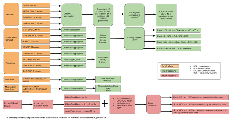
Figure 4 Flow chart describing methods used to construct population and land area along an urban continuum in low-elevation coastal zones (LECZs).

2.5.1 Elevation

The LECZs are constructed from elevation data with one main rule applied to them: contiguity to coastline. We construct two zones – below 5 m (including 5.0 m and where below 0 m is rounded up to 0 m) and 5–10 m (including 10.0 m) contiguous to coast – and compare these with all other areas within a country, that is, those areas above 10 m (or at or below 10 m but not contiguous to coastline). The ≤ 10 m LECZ is constructed by combining the ≤ 5 and 5–10 m zones.

Elevation data from four sources were used, each projected to the WGS84 horizontal coordinate system with EGM96 geoid heights: MERIT DEM (http://hydro.iis.u-tokyo.ac.jp/~yamadai/MERIT_DEM/, last access: 1 November 2021), SRTM (https://www2.jpl.nasa.gov/srtm/, last access: 1 November 2021), TanDEM-X (https://tandemx-science.dlr.de/, last access: 1 November 2021) and CoastalDEM (https://go.climatecentral.org/coastaldem/, last access: 1 November 2021) (see Table 1). In vertical terms, these elevation data models aim to set zero elevation at mean sea level using global datums with local variation. Out of the four DEMs evaluated, three of them (SRTM, MERIT DEM and CoastalDEM) were referenced to the EGM96 vertical coordinate system (EPSG:5773). Only TanDEM-X was not. TanDEM-X 90 m elevations are referenced to the WGS84 (G1150) ellipsoid (EPSG:4979). Therefore, TanDEM-X was converted from its native WGS84 ellipsoidal heights to EGM96 geoid heights using the gdalwarp (Geospatial Data Abstraction Library) tool. Each of these high-resolution DEMs were obtained from data distributions which followed regular but unique tiling schemes. Tiling of high-resolution raster data is often necessary to control for file size and usability (e.g., memory footprint), with the cost of complicating global-scale analyses when different data sets use their own schemes. Therefore, each of the DEMs were preprocessed into country units to enable the ultimate goal of country-scale analyses and to harmonize the objects being processed apart from their unique tiling schemes. This was accomplished by loading the elevation tiles into an Esri (Environmental Systems Research Institute) file geodatabase mosaic data set, which includes vector layers (footprints) of the input raster extents that identify the filename and location of each input.

Next, a Python script was used to clip the vectorized raster footprints by country boundaries extracted from the NID. This created country-level layers with attributes (filenames and locations) from intersecting footprints for each of the elevation sources which were used to isolate a subset list of elevation tiles belonging to a given country. Those subset lists were then mosaicked into country specific DEMs using the ArcGIS “Mosaic to New Raster” tool with the MEAN mosaic method; when a country was completely covered by a single tile, that tile was simply used without the need for a mosaic. All of the elevation data were then aggregated with the MEAN method of the ArcGIS “Aggregate” tool to a 9 arcsec horizontal resolution. The following additional steps were taken to ensure that the coastlines and coastal regions were adequately identified in our processes.

2.5.2 Determining coastal contiguity

Buffering the coastline

There is no international standard for coastlines, and administrative boundary data sets may or may not conform strictly to the physical reality of the coastline (Mcleod et al., 2010). Elevation data sets sometimes include representations of coastlines, but this too may differ between sources: for example, SRTM, MERIT DEM and TanDEM-X use a different implied coastline beyond which elevation is assumed to be zero, but CoastalDEM does not. This discordance in the definition of a coastline occurs for many reasons including (1) administrative boundaries that intentionally include water bodies for which there is jurisdiction; (2) coarse-scale administrative boundaries that are likely to be imprecise with respect to the physical coastline; and (3) the nature of physical coastlines to change over time (daily, monthly and yearly), which impacts both administrative and elevation sources based on the date of their data capture.

The problem of coastline disagreement is compounded for gridded data, where precise vectorized coastlines are pixelated in accordance with the raster resolution. The NID used in this study to represent coastlines has a native resolution of 30 arcsec, which implies some imprecision. However, the NID was used so that zonal statistics of population grids could capture and not double-count every populated pixel in one and only one country. In this analysis, where the overlay of the administrative data with elevation data at the coastline matters for estimation, alignment between the input spatial layers is paramount. This is particularly true for those small island nations where the majority of their land area is coastal and therefore mismatches can lead to substantial misestimating of land area and population in the LECZ.

In order to prevent the loss of population due to coastline mismatches or the loss of LECZ land area when the elevation data source uses a coastline that is seaward of the NID, the NID is buffered by 1 km on a per country basis in order to create an inclusive coastline definition which accounts for imprecision. Examples of these problem areas – and with and without this buffer – are shown in Fig. 5 for the case of Sri Lanka. The inclusive version was utilized in this work.

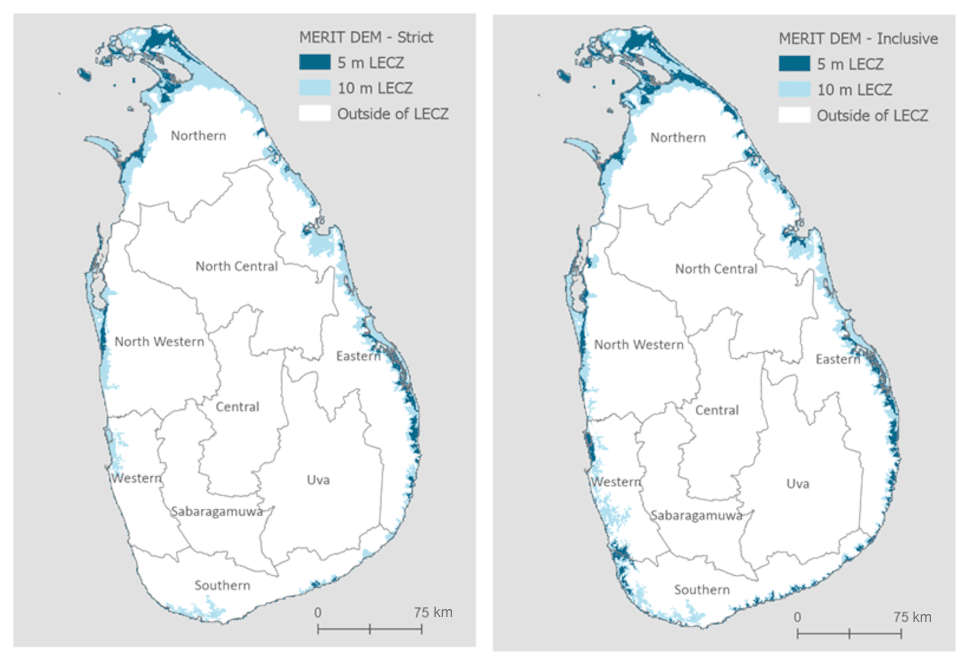
Figure 5 MERIT DEM LECZ constructed strictly and inclusively (with 1 km buffer), Sri Lanka.

2.5.3 Isolating coastally contiguous regions

The 9 arcsec country elevation mosaics for each elevation source were reclassified into integers for the following zones: ≤ 5, 5–10 m and greater than 10 m. For example, all continuous values less than or equal to 5 were assigned a value of 5; all values greater than 5 and less than or equal to 10 were assigned a value of 10; and all values greater than 10 or not contiguous to coast below 10 m were assigned an arbitrary value of 31. The reclassified images were extracted by attribute into ≤ 5 and ≤ 10 m rasters and were then segmented with the ArcGIS “Region Group” tool with eight neighbors using the WITHIN parameter. Region-grouped images are those where groups of pixels with like values are combined such that each connected group (region) receives its own unique identifier along with a count of the number of pixels within the grouping (for example see the cute cat picture in Appendix Fig. B1). In order to isolate coastally contiguous regions, the region-grouped images were converted into polygons and selected by location where each polygon intersected the border of a country as determined from the 1 km buffered NID. This effectively isolated all regions connected to administrative boundaries. Since this could potentially include inland areas, each of the files were visually inspected in order to identify spurious lowland areas contiguous with inland country boundaries (although laborious, this quality check was completed within 1–2 d of effort). When errors were discovered, they were manually removed. The isolated, quality-assured regions were then used as extraction masks on the reclassified DEMs, and null inland values were coded as above 10 m (the corresponding value in our resulting spatial data is coded as 31). The resulting rasters contained coastally contiguous pixels coded into ≤ 5 and 5–10 m LECZs and a third category representing the area outside of LECZs. Figure 6 shows the final LECZ designations for Bangkok, Thailand, by elevation source.

Figure 6 Low-elevation coastal zones (LECZs) constructed from source DEMs, Bangkok and surrounding areas, Thailand. Note that the darkest blue indicates ocean, and gray boundaries indicate first-order administrative boundaries.

2.5.4 Population

As introduced in Table 2, four population sources were utilized: GHS-POP (1990, 2000 and 2015), GPW (1990, 2000 and 2015), WorldPop (2000 and 2015) and LandScan (2000 and 2015). The horizontal resolution of these data sets vary: WorldPop is 3 arcsec; GHS-POP is 9 arcsec; and both GPW and LandScan are 30 arcsec. Therefore, methods for constructing comparable resolution population data sets and subsetting into countries varied as follows: (1) WorldPop was aggregated from 3 to 9 arcsec using the ArcGIS Aggregate tool with the SUM method and then subset; (2) GHS-POP was simply subset at its native 9 arcsec resolution; and (3) GPW and LandScan were uniformly disaggregated by a factor of 100 (e.g., 1 pixel was divided into 100 pixels, given its 1 km resolution) and quality-assured to have the same total population before and after the sampling, then subset by country. Population distributions shown in Fig. 2 represent these data processed to 9 arcsec (nominally 300 m) resolution.

2.5.5 Urban proxy

Official UN urban population statistics (United Nations, 2018) are based on the very wide range of country-specific procedures for classifying areas as urban. This variation in urban definitions presents significant challenges in making international urban comparisons. Further, these statistics do not correspond to a spatial data set, making it impossible to use with spatial data to estimate urban (or rural) populations residing in the LECZ. Thus, leveraging recent global efforts (e.g., Dijkstra et al., 2020, 2019; Pesaresi et al., 2019; Florczyk et al., 2019; Small et al., 2018a; Corbane et al., 2019; Balk, 2009) and precedent used in McGranahan et al. (2007a), we rely on satellite depictions to distinguish settlements and places along an urban–rural continuum. As in Table 3, four data sources were used: GHS-SMOD (https://ghsl.jrc.ec.europa.eu/ghs_smod2019.php, last access: 1 November 2021), GHS-BUILT (https://ghsl.jrc.ec.europa.eu/ghs_bu2019.php, last access: 1 November 2021), GRUMP (https://sedac.ciesin.columbia.edu/data/set/grump-v1-urban-extents, last access: 1 November 2021) and dLIGHT (https://sedac.ciesin.columbia.edu/data/set/sdei-viirs-dmsp-dlight, last access: 1 November 2021). The horizontal resolution of GHS-BUILT is 9 arcsec; dLIGHT is 15 arcsec; and both GHS-SMOD and GRUMP are 30 arcsec. All of these data sets were natively in the WGS84 coordinate system except for GHS-BUILT, which is natively in the world Mollweide equal-area projection. As with population, these data were conditioned into a common 9 arcsec horizontal resolution through uniform upsampling but using a nearest-neighbor approach, since the underlying data are categorical. GHS-BUILT was also projected into the WGS84 coordinate system with nearest-neighbor cell assignment at 9 arcsec. All of these data sets were subset by country using the NID.

2.5.6 Constructing classes along an urban–rural continuum

While the underlying urban-proxy data (Table 4) are continuous or ordinal along many classes, for the purposes of our summaries here we constructed three simplified, common thematic categories: urban, quasi-urban and rural. It was not possible to do this for the GRUMP data set, which includes only two classes, described urban and rural, but which is nonetheless summarized here in order to compare with the benchmark study by McGranahan et al. (2007a), which was the first of its kind to delineate urban population in the LECZ.

It is worth noting that this represents an important improvement from estimates in McGranahan et al. (2007a) and that newer, more recent estimates of global populations in the LECZ (Kulp and Strauss, 2019, which showcases CoastalDEM) do not stratify by any urban–rural classes. Other studies have highlighted population in case-study cities (Small et al., 2018b; Ahmed et al., 2018; Khan et al., 2019), but these are not global in extent; others have focused on types of cities (such as ports, De Sherbinin et al., 2007, or megacities, Nicholls, 1995) at risk.

In creating a globally applicable urban–rural categorization, inserting a quasi-urban category serves to acknowledge an urban–rural continuum and explicitly separates out a hard-to-classify and rapidly evolving but not especially large, middle range of localities. Historically, emphasis on cities – and large ones at that – has been not only in part because these localities are populous but also arguably consistent in some basic aspects of form (largely built-up, for example, or with population densities above a given threshold), which makes them easier to identify in imagery (Imhoff et al., 1997; Schneider et al., 2010). Similarly, areas identified as rural have a largely consistent signature (Doll and Pachauri, 2010). Debate arises over the treatment of the heterogeneous collection of places such as small towns, suburbs and peri-urban settlements. Whether these should be considered urban is open to interpretation and may not be discernible using features like nighttime lights, population density and built-up area. Many countries, for example, include administrative criteria or use others based on country-specific criteria in their identification of urban areas (United Nations, 2018). While such variation undermines international comparability, it can make the classification more useful locally. Variation also exists, however, among urban–rural allocation procedures designed to be internationally comparable, such as those included here, and remains even when this variation is mitigated somewhat by introducing the category of quasi-urban.

GHS-SMOD was dissolved using the ArcGIS “Reclassify” tool from its native seven classes of settlement (level 2 classification), into three classes: urban, quasi-urban and rural. This type of aggregation is inherent to the GHS-SMOD data set as the level 1 classification structure (Florcyk et al., 2019). GHS-BUILT is made up of estimates of the built-up percentage in a given 9 arcsec pixel. The raw GHS-BUILT data were thresholded into urban (> 50 % built-up), quasi-urban (> 3 % and ≤ 50 % built-up) and rural (≤ 3 % built-up) using the ArcGIS Reclassify tool; as 3 % built-up is used as a delineation of classes in GHS-SMOD that fall into the quasi-urban class, we used here for the threshold of GHS-BUILT as well. dLIGHT (Small and CIESIN, 2020) is made up of digital numbers (dn), from 0 to 255, which represent the relative luminosity of pixels across the time periods represented in the data set (1992, 2002 and 2013). Cross-classifying this with other urban depictions was done by visually comparing dLIGHT with GHS-SMOD and GHS-BUILT to find areas of agreement to guide thresholding. Based on this, the raw dLIGHT data were thresholded into urban (> 100 dn), quasi-urban (> 3 and < 100 dn) and rural (< 3 dn) using the ArcGIS Reclassify tool.

Table 4 Urban-proxy data sets: specifications of underlying inputs classification schema.

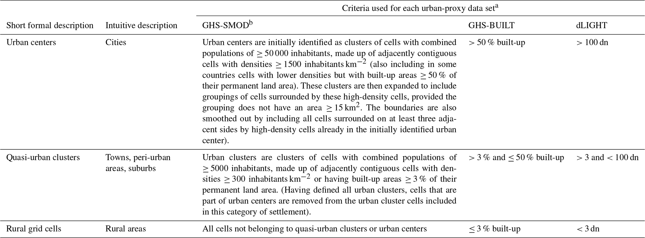
^a GRUMP Urban Extents Grid is constructed as a dichotomous urban–rural grid. Due to its construction, it is known to include a lot of land area that might be classified as quasi-urban (peri-urban and suburban-type areas extending beyond core urban areas). ^b The quasi-urban cluster for GHS-SMOD consists of that data set's classification of an urban cluster. At the time of this study, the algorithm that produces GHS-SMOD applied an adjacency rule for urban centers and urban clusters that was based on four connected cells. More recent versions of that algorithm use eight cells and rules about diagonal connectivity, though those rules have yet to be applied to a publicly available version of GHS-SMOD. See additional detail on the Degree of Urbanisation (GHS-SMOD) construction in Florczyk (2019) and about new and future updates on the data provider's website.

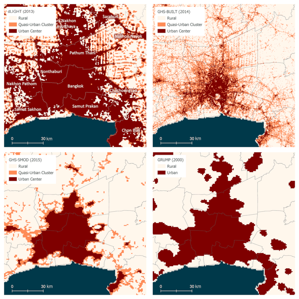
Figure 7 Urban-proxy data classified into urban, quasi-urban and rural, Bangkok and surrounding areas, Thailand. Note that the dark blue indicates ocean, and gray boundaries indicate first-order administrative boundaries.

2.5.7 Other data sets

The GPW land area grid had a native horizontal resolution of 30 arcsec. It was uniformly upsampled to 9 arcsec resolution by a factor of 100 and quality-assured to have the same total land area per pixel both before and after the sampling; then it was subset by country. The Mean Administrative Unit area grid also had a native horizontal of 30 arcsec, but because the values in this grid represent the average size of input population units, there was no need to alter or disaggregate the data values when increasing the cell size resolution. These data were simply resampled at 9 arcsec resolution and subset by country. GHS-BUILT was used here not only to discriminate between urban, quasi-urban and rural as a categorical data set but also to summarize built-up densities as a measure in its own right. It was projected from the world Mollweide projected coordinate system into WGS84 coordinates using the nearest-neighbor approach at 9 arcsec and subset by country.

2.5.8 Calculating summary statistics

We produce estimates for each of the permutations of these 12 sources using the ArcGIS “Zonal Statistics as Table” tool, by country. A Python script was then used to compile these data into a single master table. These tabular data are summarized for the globe in this section and are available along with spatial data and a Python notebook demonstrating how to produce LECZs at https://doi.org/10.7927/d1x1-d702 (CIESIN and CIDR, 2021).

We used 9 arcsec as the horizontal resolution of analysis, despite the native resolutions of elevation data nominally being 3 arcsec. The reason for this is in order to leverage GHSL layers, which are the only data sets which have data for three points in time, without simply applying growth rates to a single spatial structure. GHSL's native resolution is 9 arcsec (roughly 300 m at the Equator).

3 Results

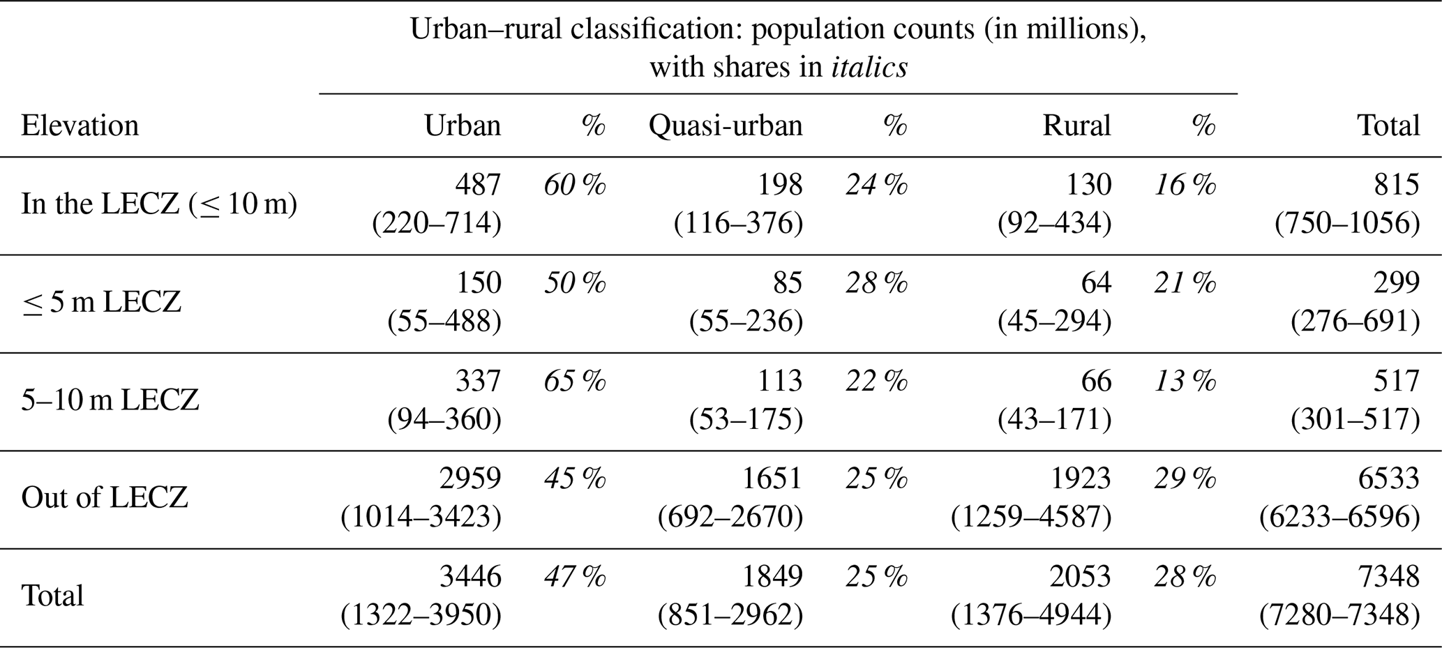
Using our core data sets as described above (MERIT DEM, GHS-POP and GHS-SMOD), we find that for 2015, 815 million persons globally live in the ≤ 10 m LECZ, with nearly 300 million of those persons living in the higher-risk ≤ 5 m zone. About 60 % of the population of the LECZ live in locations classified as urban, and another 24 % live in quasi-urban areas. Outside the LECZ, by way of contrast, the population is only 45 % urban, while the share that is quasi-urban is comparable to that in the LECZ, at 25 %. The finding that the LECZ is disproportionately urban is robust across all data combinations of input data, as shown in Table 5 and Figs. 8–15 below; however, the range of these estimates varies substantially by the choice of data sets. Thus, in the following sensitivity analysis, we aim to understand the differences in these estimates, highlighting areas of agreement as well as divergence, and to draw out the implications where possible (the full range of global estimates by elevation source, population source and urban proxy is available as summary tables with the data download).

Table 5 Summary of estimates of the global population in the LECZ, by LECZ and urban–rural classes. Core data sets (2015) shown with the range of estimates from other data sets given parenthetically.

In the discussion that follows, we first review the results for data sets within a given domain (elevation, population and urban classification) but then use only the core data set when adding dimensions. Results with full permutations are found in the data set (https://doi.org/10.7927/d1x1-d702, CIESIN and CIDR, 2021).

3.1 Comparing population and land area estimates of LECZ with different elevation data sets

3.1.1 Land area estimates by LECZ and elevation source

Figure 8 shows that for the ≤ 5 m LECZ, CoastalDEM assigns the highest percentage of land area and almost a third more land than MERIT DEM, SRTM and TanDEM-X. In the 5–10 m LECZ CoastalDEM, SRTM and TanDEM-X all assign the same percentage (0.83 %) of land area, whereas MERIT DEM allocates almost a quarter more (1.02 %). As a whole, CoastalDEM estimates the highest total land area falling within the ≤ 10 m LECZ, followed by MERIT DEM, SRTM and TanDEM-X.

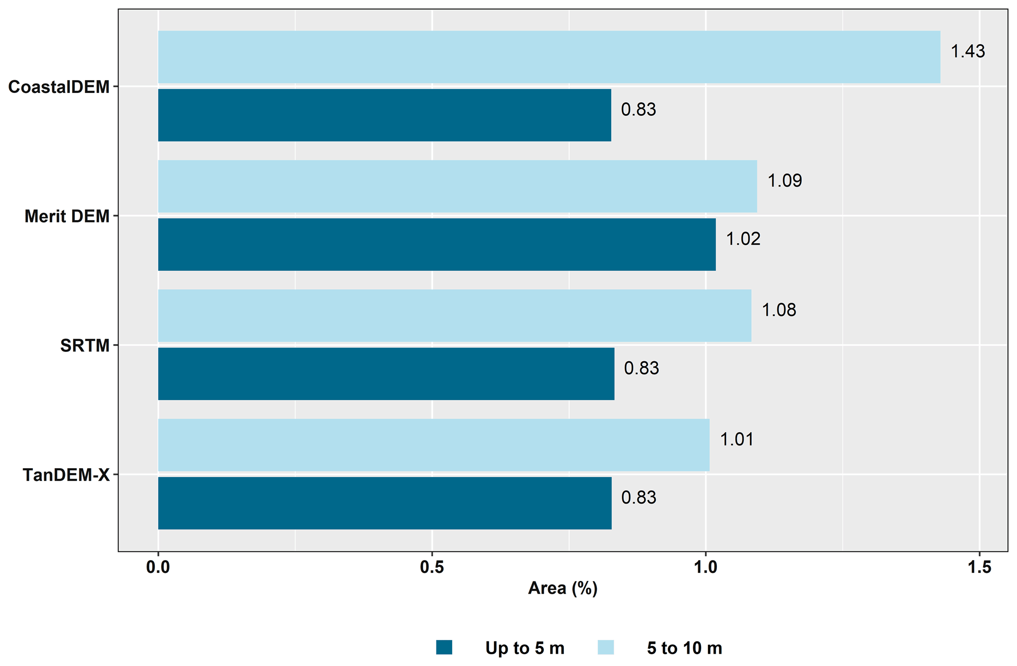
Figure 8 Percentage of total land area in the ≤ 5 and 5–10 m LECZ, by different elevation sources.

3.1.2 Population estimates by LECZ and elevation source

Estimates for the global population residing in the LECZ, by different elevation and population data sources, are shown in Fig. 9 for 2015 and Appendix Fig. B11 for 1990. The shares of population residing in either the ≤ 5 m LECZ or the 5–10 m LECZ have increased somewhat in the past 25 years, irrespective of which elevation data source is used to estimate the LECZ or which population estimates are used (only GPW and GHS-POP have estimates for 1990). Depending on the data sources, an additional 0.25 % to 0.49 % of the world's population was living in the ≤ 10 m LECZ in 2015 than in 1990, which equates to ∼ 20 000 000–40 000 000 more people.

Figure 9 shows the impact of population data choice on estimating the percentage of people living in LECZs globally in 2015. The relationship is clear to discern in the 5–10 m LECZ, where GPW consistently estimates the lowest percentage, with WorldPop being the second lowest, LandScan being the third lowest and GHS-POP being the highest percentage regardless of the elevation source used to define the LECZ.

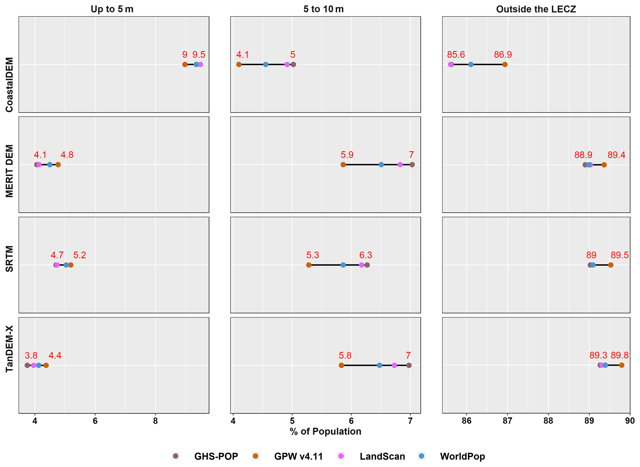
Figure 9 Estimates of population in different LECZs, by elevation and population data sources, 2015.

Based on Fig. 9, it is clear that the selection of an elevation source has a greater impact on the estimation of population (and land area) in the zones than the selection of a population data source itself. The largest difference (in percentage points) between population sources is for areas outside the LECZ: using CoastalDEM for elevation there is a 1.3 % difference between LandScan and GPW. This is the largest difference in the percentage of population estimated inside or outside the LECZ within any single elevation data source. The combined largest difference across all categories of elevation and population is 5.7 % when comparing CoastalDEM and TanDEM-X in the ≤ 5 m LECZ, where TanDEM-X estimates 3.8 % using GHS-POP and CoastalDEM estimates 9.5 % using LandScan. Nevertheless, the selection of a population data source on its own is significant when considering that a difference of even 1 % globally between sources amounts to approximately 80 million people in 2015. Also, since these differences in LECZ shares are not uniform, within some local areas the selection for population data may have considerably more impact.

3.1.3 What is driving the differences?

Considering only GHS-POP 2015 population estimates (without stratifying the urban–rural continuum), by using CoastalDEM, we estimate that 687 million people live in the ≤ 5 m LECZ globally, whereas when the other data sets are used we estimate far fewer – 299 million with MERIT DEM, 346 million with SRTM and 276 million with TanDEM-X – people live in that same zone. Why is there such a large discrepancy? First and foremost, as indicated in Fig. 8, the land area of the ≤ 5 m LECZ is about 40 % more in CoastalDEM than in the others.

Looking at the endmembers of this range of estimates (CoastalDEM on the high end and TanDEM-X on the low end), roughly 80 % of the population difference can be found across 11 countries (China, India, Bangladesh, Indonesia, Viet Nam, Japan, Philippines, Egypt, Thailand, United States of America and Brazil), and more than 30 % of this difference occurs in a single country, China, where CoastalDEM predicts approximately 184 million people in the ≤ 5 m LECZ and TanDEM-X predicts approximately 54 million. A closer inspection of the elevation data sets sheds light on how these two data sets vary in their detection of low-lying areas.

Figure 10 Comparison of LECZ data sources along the Yangtze River, China, for CoastalDEM and TanDEM-X elevation sources. Basemap from Esri, DigitalGlobe, GeoEye, Earthstar Geographics, CNES/Airbus DS, USDA, USGS, AEX, Getmapping, Aerogrid, IGN, IGP, swisstopo and the GIS User Community.

Figure 10 shows differences in the evaluation of coastal contiguity. In the right-hand panel, the CoastalDEM elevation data source extends inland up the Yangtze River, which leads to identification of low-lying areas near Hefei and Nanchang which are not considered contiguous to coastline according to TanDEM-X (or MERIT DEM and SRTM). Figure 10 also shows in the left-hand panel an area near Rugao, China, where a portion of the low-lying area is not included in the final ≤ 5 m LECZ based on TanDEM-X because it is not contiguous to the coastline owing only to the fact that it is cut off by a roadway.

CoastalDEM sets all grid cells over inland water to an elevation of zero; therefore when we evaluate coastal contiguity, the contiguous coastal zone extends further inland (e.g., to include more river tributaries) than with other data products which have variable elevation values over inland water which sometimes exceed 5 m or 10 m. This partly explains why more inland areas are captured within the LECZ by CoastalDEM than the other sources. The LECZ based on TanDEM-X produces the smallest estimates of population. Unlike the other elevation data, it detects roads (notably found at higher density in urban settings) and classifies them as being at higher elevation than their surroundings as shown in Fig. 10 above (and it is overall more sensitive to built structures and other elements of the landscape than the other elevation data sources). This is especially relevant when constructing LECZs because in the evaluation of coastal contiguity, we require direct connectivity to the coastline. Because TanDEM-X classifies roads (and other features) at higher elevation than their surroundings, it effectively creates contiguity barriers and thus smaller ≤ 5 and ≤ 10 m LECZs. Similar phenomena are observed when considering MERIT DEM or SRTM, namely that raw elevation estimates in these sources sometimes produce barriers which prevent coastal contiguity. (Whether these barriers indeed function as higher-elevation impediments to flooding is an open question that local studies may be able to address; Orton et al., 2015, 2020.) The CoastalDEM model produces a more homogenous surface which therefore expands the zone of contiguity to the coast, which increases the land area and population estimates within the zone (see Appendix Fig. B2).

3.2 Comparing population and land area estimates with different urban-proxy data sets

3.2.1 Land estimates by urban classes

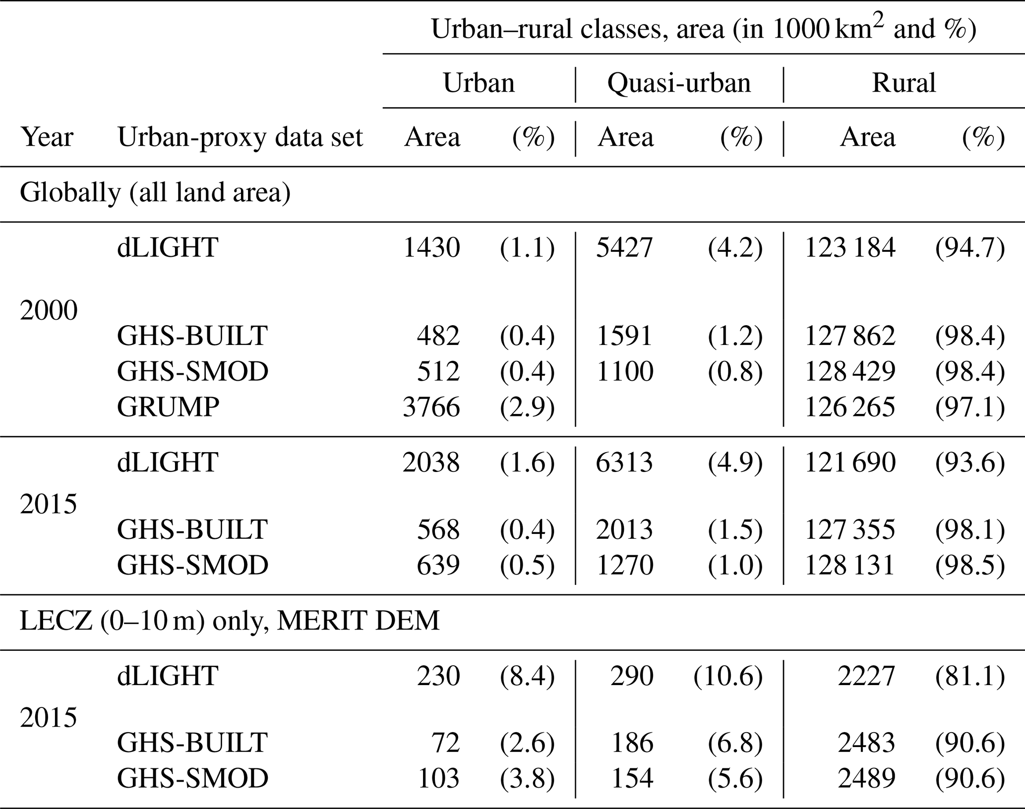
Before evaluating the population in the LECZ along the urban–rural continuum, it is helpful to see how the different urban-proxy data sets differ in their estimation of land area. Table 6 shows estimates of land area for the years 2000 (so that the comparison to GRUMP can be made) and 2015. The GRUMP data, sometimes criticized for the blooming quality inherited from the use of the stable city lights as a key input (Nowak Da Costa et al., 2017), can be taken to combine the urban and quasi-urban categories into urban only; at least this is observed when comparing with urban and quasi-urban data not based on city lights. Combining urban and quasi-urban areas, for year 2000, the results according to dLIGHT are the most inclusive (5.3 %) estimates of global land area, followed by GRUMP (2.9 %), then GHS-BUILT (1.6 %) and finally GHS-SMOD (1.2 %). The same general pattern is seen for the year 2015, when GRUMP is omitted; additionally, changes over time in total area and percentages are also detected. These different urban proxies produce somewhat different depictions of land area. However, we find fairly strong agreement in the land area estimated in the urban class between GHS-BUILT and GHS-SMOD. This is not surprising because they share an important underlying data source (GHS-BUILT), but dLIGHT (like GRUMP before it) places more land area in both urban and quasi-urban classes, which is also not surprising, as both GRUMP and dLIGHT are based on nighttime lights which have known blooming effects.

Table 6 Land area of urban, quasi-urban and rural by urban-proxy data sets.

3.2.2 Population estimates by urban classes

The UN World Urbanisation Prospects project estimates that in 2018, 55 % of the world's population lives in urban areas (United Nations, 2018), and whether this estimate is accurate or not (Cohen, 2004), it remains the established benchmark of urban population statistics. Since the UN's estimate is derived from collections of country-specific urban measurements, the open questions are whether globally consistent and spatially derived estimates are in fact more accurate and whether or not these agree with the UN's estimates. Without additional information, we cannot evaluate accuracy, but we can characterize whether or not there is agreement.

Using these globally consistent urban-proxy data sets, we show in Fig. 11 the share of the population that resides in urban, quasi-urban or rural settlements in 2015. The top panel of Fig. 11 shows the variation in the estimates by data source along this continuum. For any given population data set, the total population sums to 100 % across the urban, quasi-urban and rural classes. In general, GHS-POP concentrates more people into urban and quasi-urban categories, no matter which urban-proxy data set is used, and GPW concentrates more people into the rural category no matter which urban proxy is used. In terms of comparison to the UN estimates, whether the percentage of the population estimated to be urban shows agreement with the UN's estimate depends both on which urban proxy and which population data set are used. GHS-POP and LandScan place at least 55 % of the population (and sometimes, quite a bit more) in urban and quasi-urban areas regardless of which urban-proxy data are used, whereas WorldPop (except when using dLIGHT) and GPW place less than 55 % of the population in urban and quasi-urban areas. Use of dLIGHT as an urban-proxy data set leads to comparable or higher proportions of the population in urban and quasi-urban areas across all population data sources. Importantly, none of the population data sources, irrespective of the urban-proxy data set, place 55 % of the population in areas classified as urban only; however when combined with quasi-urban, they do approach 55 %. Similarly, irrespective of the urban-proxy data set, the percentage of the global population in urban and quasi-urban areas has grown substantially since 1990 (see Fig. B12).

Perhaps it is not surprising that estimates of population in rural areas vary more than those in urban areas, because satellite data broadly agree on the urban category due to its relatively consistent and identifiable morphology. Most notably, the ranges in rural areas are largest when using GHS-BUILT or GHS-SMOD. The ends of these ranges are GPW, which uses no modeling towards settlements (or other attributes), and GHS-POP, in which the population reallocation is dominated by settlements (but not other ancillary features). Additionally, GHS-BUILT produces the widest range of population estimates across the three urban classes; in other words, the GHS-BUILT urban proxy is highly sensitive to the choice of population data.

Figure 11 Percent of total population, by urban–rural classes, using different urban-proxy and population data sources, globally and in the ≤ 10 m LECZ (using MERIT DEM) 2015.

3.2.3 Population estimates by urban classes in LECZs

In comparison to the global distribution, the lower panel of Fig. 11 identifies the population distributions along the urban–rural continuum in the ≤ 10 m LECZ (using MERIT DEM): the denominator in this panel is the total population in the LECZ. It is clear that the population is more concentrated in urban areas in the ≤ 10 m LECZ than globally. For instance, using GHS-SMOD as the urban-proxy and GHS-POP population data, less than half – 47 % of the global population – reside in the urban class, in contrast to in the ≤ 10 m LECZ, where 60 % of the population lives in urban areas. Similarly, the population of the LECZ is less rural than the global average. Indeed, compared to the global figures, the urban population shares in the ≤ 10 m LECZ are higher, and the rural shares are lower for all combinations of population and urban-proxy data sets (and for all the elevation data sources, as shown in the summary tables available with the data download). However, the quasi-urban population shares are sometimes higher and sometimes lower in the ≤ 10 m LECZ than globally depending on which population and urban proxy are used. For each of the urban proxies, the estimates of the quasi-urban shares based on the different population data sets are closer to each other within the ≤ 10 m LECZ, though the ordering remains the same as global, with GHS-POP having the highest quasi-urban share and GPW having the lowest (as for urban).

Comparing the upper and lower panels of Fig. 11, it is clear that the range of estimates of the population share for each urban class is narrower in the LECZ than the respective global ranges. This is likely because the LECZ is itself more urban, and urban areas are where the resolution of the underlying census data is finest. (See Appendix A1 for a discussion of the role of underlying resolution on the population.) Similarly, all of the urban proxies show less sensitivity to the choice of population data set within the LECZ than they do globally, and both GHS-SMOD and dLIGHT show the least sensitivity in the quasi-urban class both inside the LECZ and globally. Notably, as shown in the lower panel of Fig. B12, the same patterns held in 1990, when the combined urban and quasi-urban population shares in the LECZ exceeded 50 % (for all combinations of data sets except one). Whether population shares in the urban and quasi-urban areas of the LECZ have increased more than those shares globally is a question we address below.

Taking a closer look at the distribution of population within the LECZ, the pie charts in Fig. 12, shown using only MERIT DEM and GHS-SMOD, reveal some other interesting patterns (including information necessary to understanding the fractions of the population in the LECZ and their associated densities). (1) The population data sets vary in the total number of persons estimated to reside in the LECZ. GHS-POP places the greatest number of persons in the LECZ (815 million) and the least in GPW (781 million), a difference of 35 million persons. (2) Despite differences in the shares of the population estimated to live in the different urban classes (also shown in Fig. 11), the ratios of population living under 5 m to that living in 5–10 m is relatively consistent across population data sets, with notably greater fractions of the urban population in the LECZ living in the 5–10 m zone. (3) Consistent with much different land areas (Table 6), the urban-proxy data sets (shown in Appendix Fig. B3) reveal different distributions of population in the LECZ.

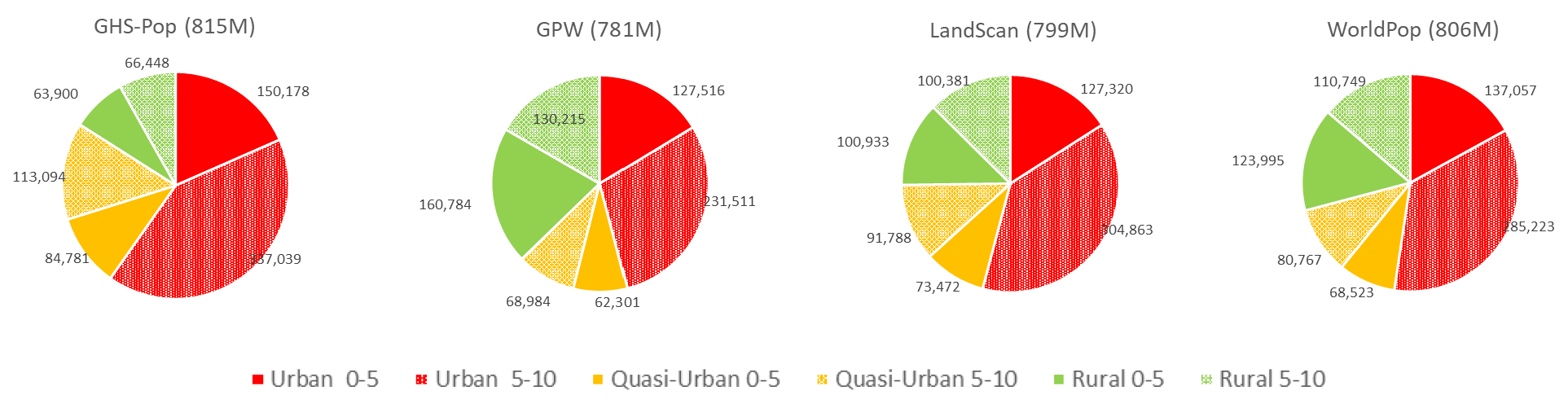
Figure 12 Proportion of the population in each urban class (urban, quasi-urban and rural) in the ≤ 5 and 5–10 m LECZ, for different population data sets, 2015. Shown using GHS-SMOD as the urban proxy and MERIT DEM for LECZ delineation. Labels indicating population count (in thousands) are shown.

Given the comparably high shares of urban population in the LECZ, Fig. 13 shows the urban (or quasi-urban or rural, respectively) population that resides in the ≤ 10 m LECZ as a proportion of the global total in each respective urban–rural class (using MERIT DEM and GHS-SMOD with full results shown in Appendix Fig. B3). Even though GPW estimates the smallest population in the LECZ and the smallest urban population both globally and in the LECZ, it estimates the highest proportion of total urban population in the ≤ 10 m LECZ: nearly one out of every five urban dwellers live in a city in the LECZ. This pattern holds no matter which urban-proxy data set is used. In contrast, GHS-POP estimates the largest population in the LECZ and the largest urban fractions globally but, as shown in Fig. 13, places only one out of every seven urban dwellers in the LECZ. Smaller proportions of the global rural and quasi-urban populations live in the LECZ, but particularly notable is that of the rural population in the LECZ, roughly half live in the higher-risk ≤ 5 m zone.

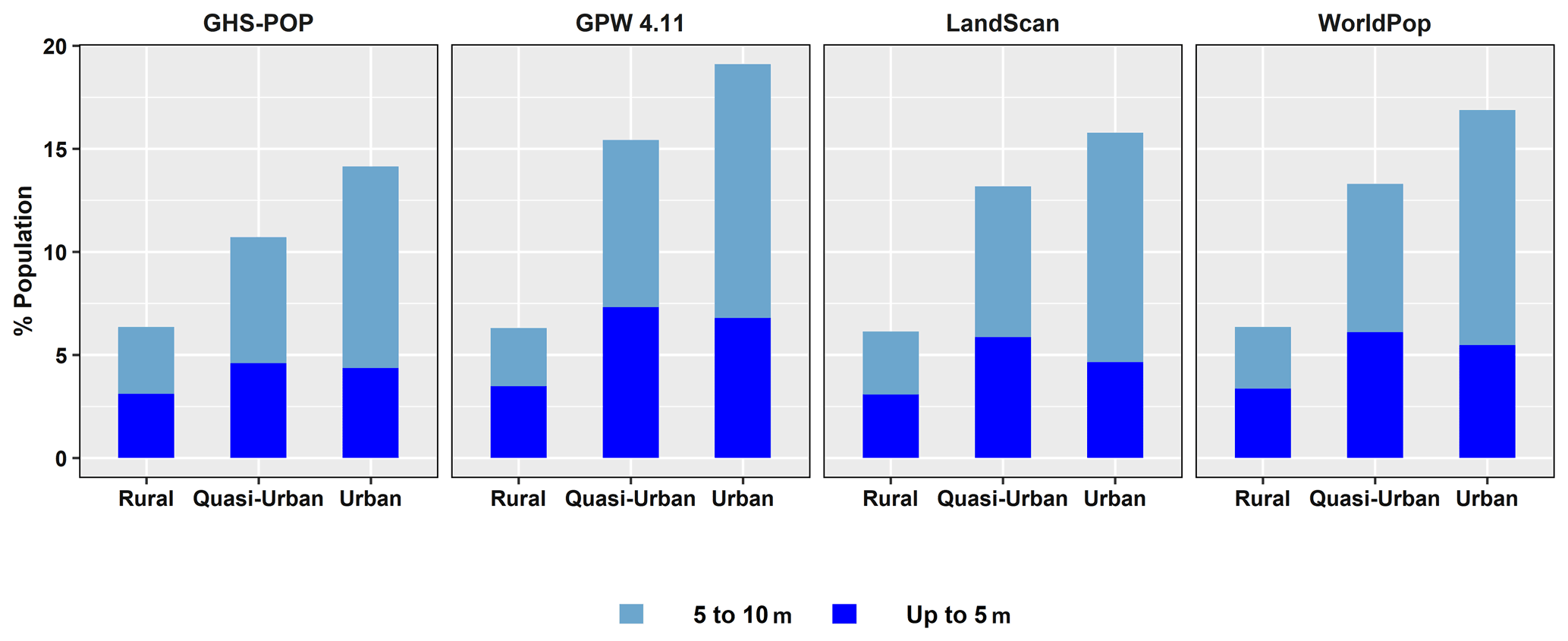
Figure 13 Percentage of the population in each urban class (urban, quasi-urban and rural) in the ≤ 5 and 5–10 m LECZ, by each respective urban–rural class, according to different population data sets, 2015. (GHS-SMOD is used for the urban proxy, and MERIT DEM is used for LECZ delineation.)

3.2.4 What is driving the differences?

Differences in the estimates of population – especially within classes along an urban–rural continuum – between urban-proxy data sets are largely driven by four factors: (1) the selection of the population data source; (2) the underlying satellite data measure and its associated urban construct; (3) the resolution of the underlying sensor; and (4) the thresholds used in the construction of urban classes – choices we have imposed for GHS-BUILT and dLIGHT and the choice to use JRC's GHS-SMOD level 1 classification (which the user community at large can continue to evaluate and revise). A fifth consideration that interacts with these factors relates to the underlying and intrinsic resolution of population data in urban areas, an issue that becomes more significant when considering the LECZ because it is disproportionately urban.

As described in Sect. 2.2, the key differences between the population data sources arise from how they allocate population within census-based geographic units. GPW distributes population uniformly within these areas, without taking any account of indications that the land is urban (e.g., built-up) or rural (e.g.,  forested). GHS-POP distributes the same populations on the basis of built structures, in effect concentrating the population in those areas more likely to be classified as urban or quasi-urban. WorldPop also distributes the same population using different indicators and is also likely to concentrate population in more urban locations. LandScan builds on somewhat different sources for its initial population inputs and uses a somewhat different model to distribute the population but is also designed to distribute more population to land with more urban characteristics. In densely populated urban areas where the underlying census units tend to be more finely resolved (even in data-poor settings), there is likely to be the greatest agreement between the population estimates across the population data sources (this is explained in more detail in Appendix A1). Where there are differences, one would expect GPW population counts to be more rural than the others. The global statistics presented above conform with this expectation. So do those for the ≤ 10 m LECZ, though the differences between the population sources are less, which is probably explained by higher overall densities and higher input resolution in coastal areas. All the population data sources estimate that the share of global urban populations located in the ≤ 10 m LECZ (using MERIT DEM) is higher than the share of the global quasi-urban population, which is in turn higher than the share of the global rural population. However, GPW has the highest shares of the urban and quasi-urban populations in the ≤ 10 m LECZ, which is notable given its particularly low urban and quasi-urban populations outside of the zone, and provides additional evidence that the zone is disproportionately urban.

The urban-proxy data sets determine which areas are classified as urban, quasi-urban and rural, using different indicators, as well as cutoff points between the classes that are inherently somewhat arbitrary, and help determine the share of land in each class. GHS-BUILT uses a physical (built settlements) model, and GHS-SMOD expands it by also using population density, whereas dLIGHT and GRUMP use the detection of nighttime lights which combine physical, atmospheric and environmental factors. In terms of application to urban locations, areas that are built are almost always included in the nightlight-based products. One of the reasons that the light-based products are more inclusive is because they contain land uses that are not built structures but which may be lit (urban parks, roads, etc.; Stokes and Seto, 2019) and that the lights “bloom” beyond the area where the actual light originates (Small et al., 2005), and while the resolution of the data underlying dLIGHT is much higher and thus reduces concern, this concern persists. While many user communities prefer the more spatially delimited built construct, others (notably ecologists) prefer light-based extent because its more expansive nature is better suited to the study of ecosystems, capturing the dynamics of land fragmentation (McDonald et al., 2011).

The input horizontal resolution of GHS-BUILT is highly refined at 9 arcsec, whereas dLIGHT has a native resolution of 15 arcsec, and GRUMP has one of 30 arcsec. The resolution of GHS-SMOD is also 30 arcsec, but it is constructed from higher-resolution (9 arcsec) input data. These differences in resolution impact the classification of areas into urban, quasi-urban and rural, since data which originated from a coarser scale are likely to be more inclusive. For example, on the edges of the urban class there are often transitions to quasi-urban which are clearly captured when using high-resolution data but are combined into the urban class at lower resolutions until greater than 50 % of a pixel is captured as quasi-urban.

The selection of thresholds that we used for the GHS-BUILT and dLIGHT data sets (as well as the use of GHS-SMOD level 1 classification) is another important factor contributing to the variation in land area estimated to be in each class. The determination of any critical values to differentiate settlement types is somewhat subjective, as evidenced by the wide range of country definitions of settlement types utilized in global censuses (United Nations, 2018). We applied thresholds here based on a limited number of other studies that have evaluated the impact of thresholds on detection (Leyk et al., 2018; Balk et al., 2018; Tong et al., 2018). GHS-SMOD is a fairly new data product as well that continues to make improvements to its model, in particular on the rules used to create the different urban classes, such as whether to apply a given built-up threshold or not. (Early work applied a 3 % threshold; the latest and stable release removes this threshold.) Future work should help to evaluate the usefulness and sensitivity of these and other thresholds.

Because estimates of land area differ in the LECZ by urban-proxy data set (as well as elevation), the last result section will evaluate differences in population (and built) density.

3.3 Comparing built-up and population density estimates by urban-proxy data sets

This section turns from comparing population and land area estimates for different LECZ and urban–rural classes to examining the related population densities and built-up area density estimates across these same classes. Population densities are simply the population counts divided by the land areas. Urban areas are associated with high population density, and indeed a high population density is often treated as a criterion to define urban areas (Solecki et al., 2015; Dijkstra et al., 2020). Having a high proportion of the land built-up is also sometimes treated as a defining feature of urban areas (Melchiorri et al., 2018; Wentz et al., 2014). Moreover, nighttime light is assumed to be associated with where human populations and built-up urban areas are located (Wentz et al., 2014; Henderson et al., 2020).

Along the urban–rural continuum, urban areas can be expected to be the most built-up, and rural areas are the least: being built-up is part of how urban areas can be identified (as is fully the case with GHS-BUILT and partially the case with GHS-SMOD), and being built-up is also generally associated with population density (used as one of several criteria to identify urban area in GHS-SMOD) and lit-up areas (used to identify urban areas with dLIGHT). While one would expect the relationship to be particularly close for the classification based on GHS-BUILT, where one would also expect it to depend on the thresholds (of the respective measure in each urban-proxy data set) chosen, with particular thresholds resulting in smaller urban areas yielding higher urban built-up shares in those areas and thresholds resulting in larger rural areas yielding higher rural built-up shares (and quasi-urban areas having higher built-up shares when urban areas are smaller and rural areas larger). Somewhat similar expectations apply to population density, though in this case the urban-proxy data set most likely to pick out high-density urban areas and low-density rural areas is GHS-SMOD because it uses population density as a criterion in the construction of the GHS-SMOD classes. Also, excessively tight thresholds could in principle reduce urban population densities, as city centers are often dominated by commercial property, exhibiting lower population densities (at least at night).

3.3.1 Built-up and population density by urban class and elevation

Figure 14 shows the global, average built-up percentage for urban, quasi-urban and rural categories across the urban-proxy data sets (i.e., this is the average concentration of built-up areas based on GHS-BUILT). GHS-BUILT is a measure of the percentage of any given pixel that is considered built-up. The urban class is on average,46.16 % built-up according to GHS-SMOD data; according to the thresholded GHS-BUILT urban proxy, the urban class has a higher concentration of built-up area, at 77.29 %; and according to dLIGHT, which produces a more expansive urban area (see Table 6), the urban class has an average built-up percentage of only 22.55 %. GHS-SMOD captures areas as rural which are a factor of 20 more built-up (0.21 %) as compared to GHS-BUILT, which only includes the least built-up of areas in the rural category (0.01 %), and dLIGHT is in between (0.08 %).

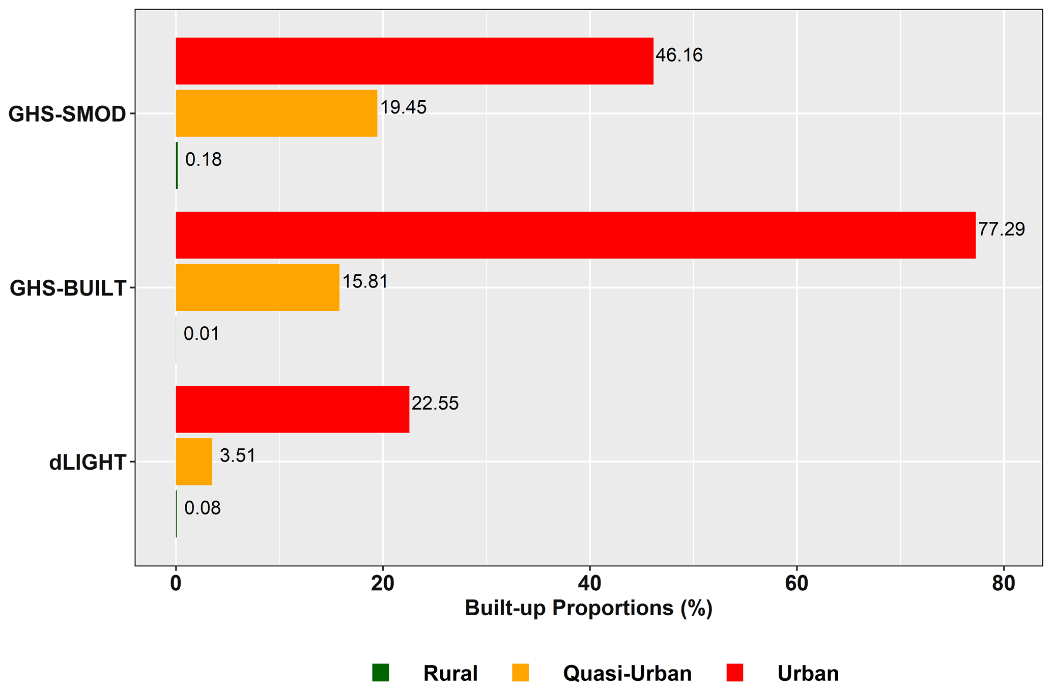
Figure 14 Built-up density of urban, quasi-urban and rural by different urban-proxy data sets, 2015.

Figure 14 can be compared to Fig. 15, which shows the same classes, but by population rather than built-up densities, for each population data source (along the x axis) and urban-proxy data set (on the y axis). The highest population densities are found, as expected, in urban areas, and these are several times those of quasi-urban areas, which are in turn several orders of magnitude greater than those in rural areas. This is similar to the built-up area differences, though for GHS-SMOD in particular the population density differences between urban and quasi-urban areas are greater than the differences in the proportion of built-up area. Within a given urban-proxy data set, the estimate of population density depends largely on which population data set one uses – and these differences between population data sets are substantial. For example, using GHS-SMOD for our urban-proxy data set, the population density in urban areas according to GPW is 2942 persons km⁻², whereas with GHS-POP it is 5393 persons km⁻². In contrast, within a population data set, the difference across the urban-proxy data sets is largely comparable between GHS-SMOD and GHS-BUILT but is substantially smaller with dLIGHT. In short – and importantly – estimates of population density depend on one's choice of both the urban-proxy data set and the population data set.

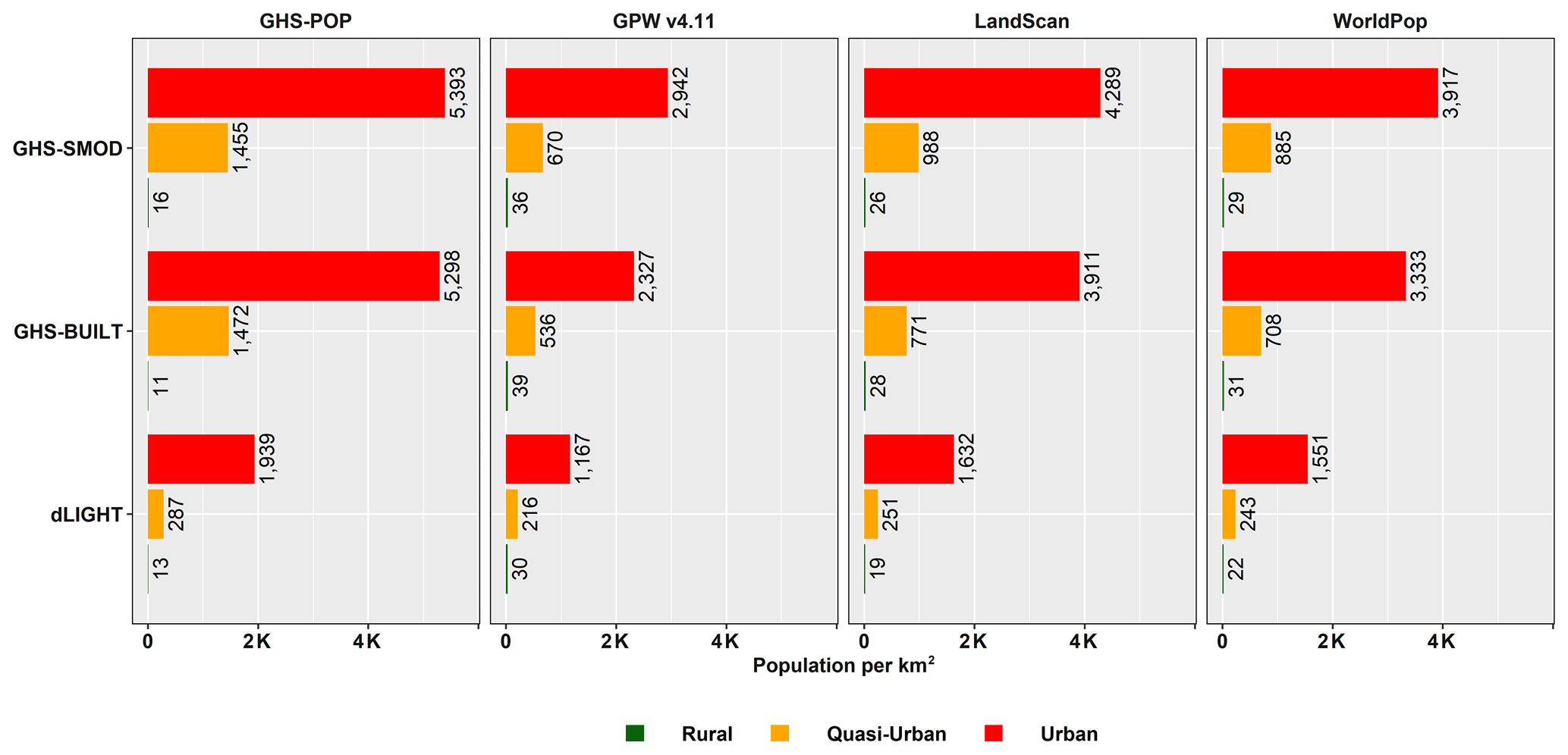
Figure 15 Population density of urban, quasi-urban and rural areas by urban-proxy data sets (y axis) and population data (x axis).

Whereas Figs. 14 and 15 show average global densities, in Figs. 16 and 17, we separate out the LECZ classes. (For simplicity, we show the LECZ based on MERIT DEM only, with the full comparison shown in Appendix Figs. B4 and B5, noting that differences are small between elevation data sets.) While there are inherent relationships between both the built-up share and population density and an area's degree of urbanization (i.e., because built-up area and population density are often taken to be defining features of urban settlement), there are no inherent relationships between either population or built-up density with elevation levels and the LECZs. Nevertheless, the ≤ 10 m LECZ is disproportionately urban, with a tendency to have higher population and built-up densities than outside of the LECZ.

Are urban and quasi-urban areas in the LECZ more built-up than areas outside of the LECZ? The answer in part depends on which urban-proxy data set is used and on differences within the zone itself. Figure 16 shows that the ≤ 5 m LECZ is less built-up than the 5–10 m LECZ, with large differences when using GHS-SMOD or dLIGHT. Notably, the built-up percentages are greater in the 5–10 m LECZ in all classes of the urban continuum than areas outside of the LECZ with the exception of GHS-SMOD, where urban areas in the 5–10 m zone are quite similar in their built densities (53.5 % vs. 55.3 % outside the LECZ). GHS-BUILT produces built-up percentages that are almost invariant across the different LECZs.

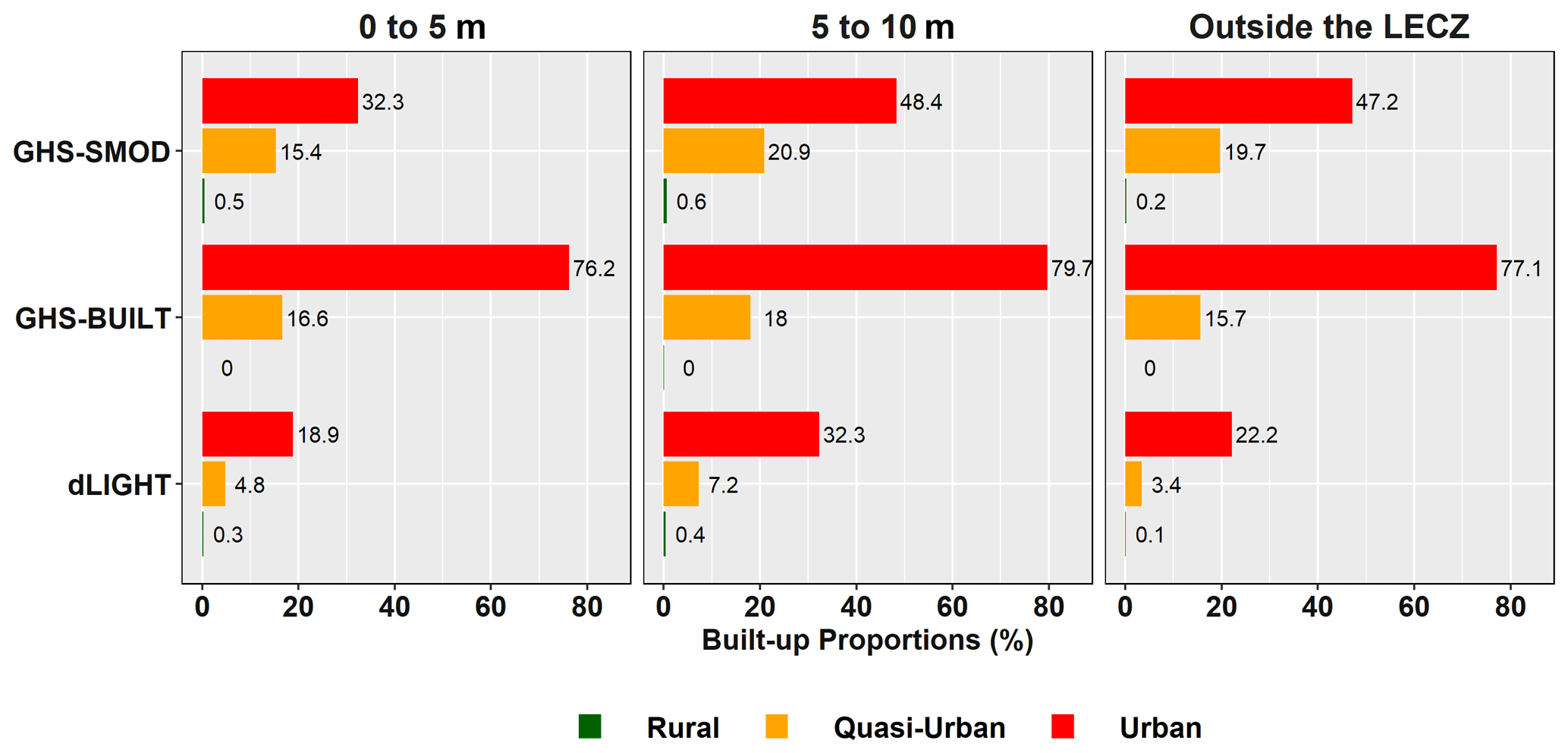
Figure 16 Built-up density (%) of urban, quasi-urban and rural areas by urban-proxy data set, using the MERIT DEM elevation source.

Like Fig. 16, Fig. 17 asks how population density varies within the LECZ and compares to areas outside of the LECZ (results shown only for GHS-SMOD with other urban-proxy data found in Appendix Fig. B5). Population densities are lowest in the ≤ 5 m LECZ, along the urban continuum (with the exception of GPW, where population densities in the ≤ 5 m zone are higher than outside of the LECZ). All of the population densities in the 5–10 m LECZ are higher than those outside of the LECZ except for GHS-POP, where the density in the 5–10 m LECZ is only slightly less than outside of the LECZ.

Figure 17 Population density of urban, quasi-urban and rural areas using GHS-SMOD, by LECZ (using MERIT DEM), according to different population data sets, 2015.

3.4 Change over time: population growth in the LECZ along the urban–rural continuum

In 1990, according to GHS-POP and GHS-SMOD 570 million persons lived in the ≤ 10 m LECZ; 25 years later, that population has grown by another 245 million persons. As Fig. 18 shows, while the population has grown everywhere in the LECZ – that is, in urban, quasi-urban and rural areas – urban areas have experienced the greatest increases. The share of the global urban population living in the LECZ has grown from 13 % in 1990 to 14.2 % in 2015, whereas the shares of the respective quasi-urban and rural areas have declined – presumably, in part because some areas that were classified as quasi-urban or rural in 1990 have transformed to urban during this period. Also notable is that the proportionate change in this 25-year period is greatest in the urban areas in the ≤ 5 m LECZ (a pattern that holds across elevation data sets).

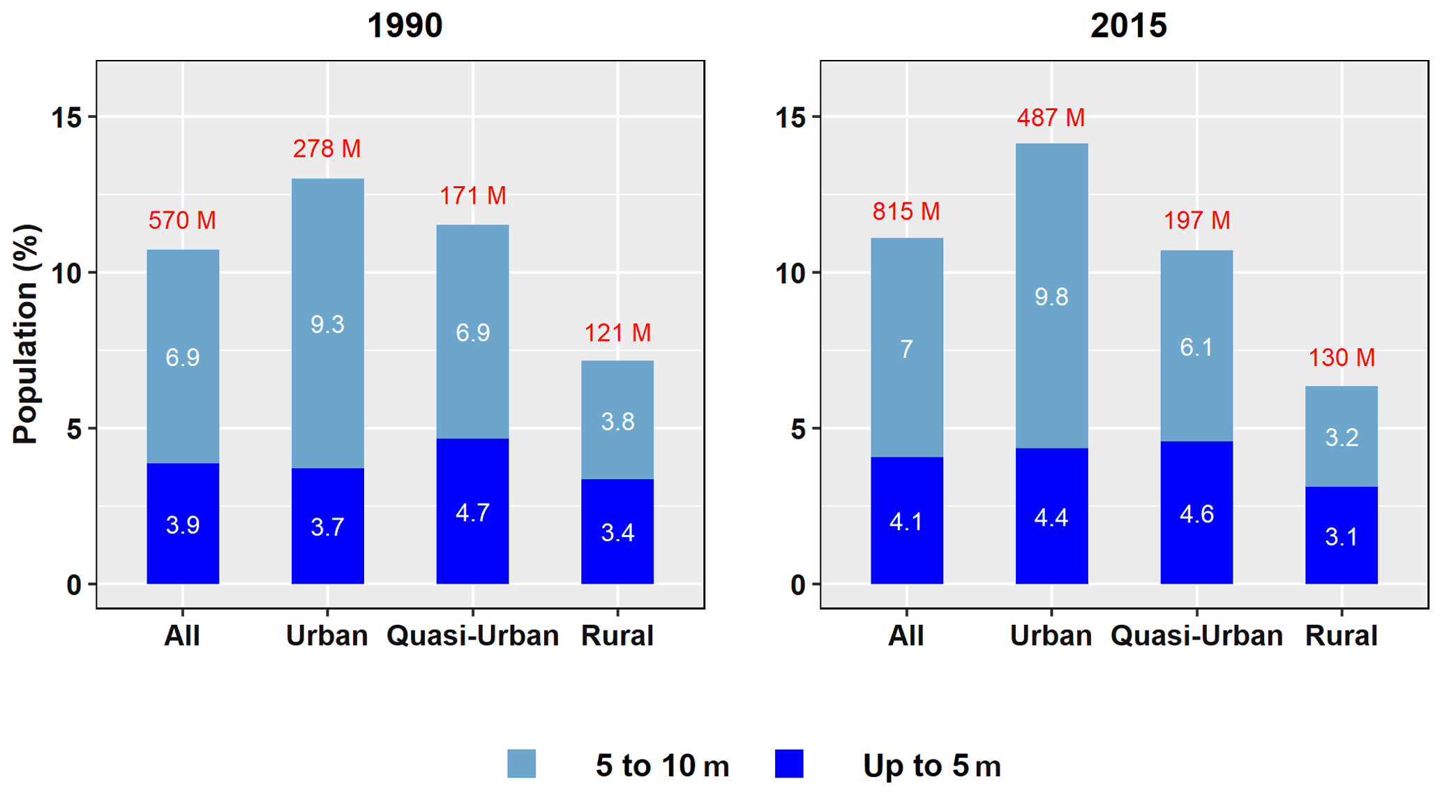
Figure 18 Respective share of population in the LECZ, by LECZ and urban–rural classes, 1990 and 2015. Core data sets used (MERIT DEM for LECZ, GHS-SMOD for urban-continuum classification and GHS-POP for population).

Has the urban population in the LECZs grown more than the urban population overall? The answer to that is yes. Table 7 shows the shares of the respective urban, quasi-urban or rural population living in the ≤ 10 m LECZ in 1990 and 2015 and their change over the 25-year period: in 1990, 11.4 % or the urban population – 1 out of every 7.7 urban persons – lived in the LECZ; by 2015, 14.1 % – 1 out of every 7.1 urban persons – lived there, using GHS-POP, GHS-SMOD and MERIT DEM, whereas the percentage of the respective populations living in quasi-urban and rural areas has fallen in these 25 years. The population living in urban areas in the LECZ has grown considerably more – ranging from a 67 % increase to more than doubling, depending on which data set one uses – than in urban areas outside the LECZ. While populations have grown in quasi-urban and rural areas, according to most data combinations, they have grown much less than in these areas outside the LECZ. While the levels of these shares differ somewhat across urban-proxy and population data sets, the main message is unambiguously consistent: urban population has grown more in the LECZ than outside of it.

Table 7 Estimates of the global population and percentage change in the LECZ by urban–rural classes (based on different urban-proxy and population data sets) for 1990–2015.

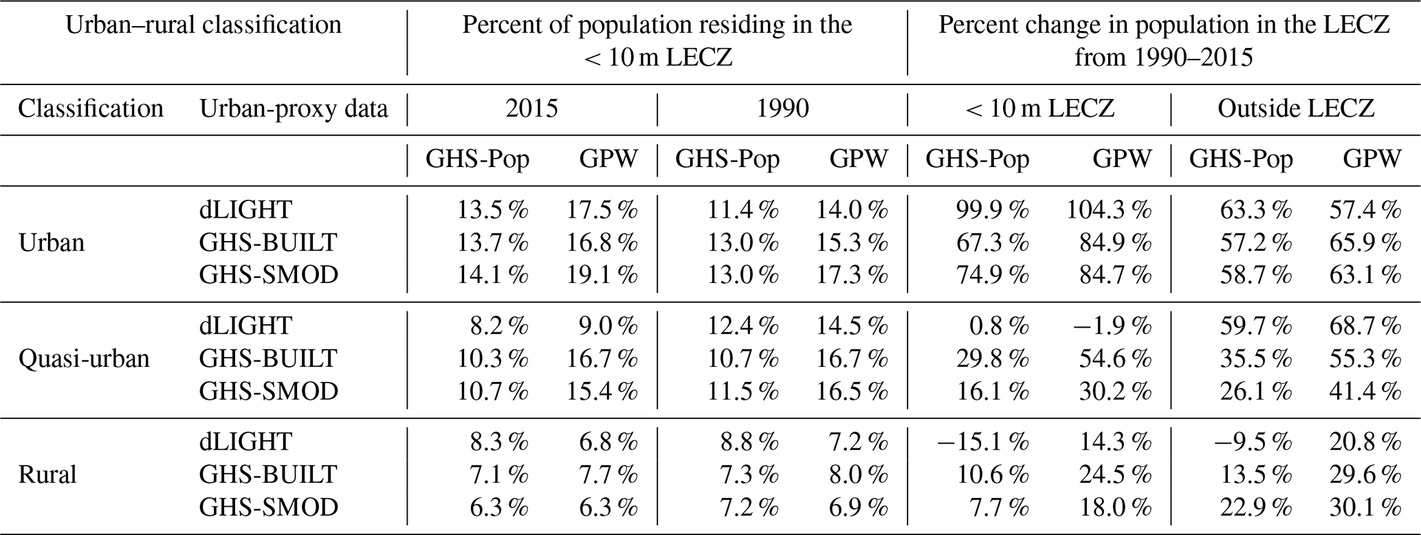
Note: MERIT DEM used as elevation data for the LECZ.

4 Fitness for use and directions for future research

When modeling three different phenomena – all imperfectly – and then combining them, it is prudent to reflect on limitations (e.g., accuracy or uncertainty) and future usages of these data, including many that go well beyond what we have described in this analysis. Following the example found in a recent review of global population grids (Leyk et al., 2019a), here we pose some questions that users of the data sets produced herein may use in order to describe fitness for and possible limitations in use. As we have made evident above, it is important to get under the hood of any given data set to understand what data went into its construction along with important modeling assumptions.

Importantly, estimates of population in the LECZ, along an urban continuum, are sensitive to the choice of data sets. For some uses, it will be important to be explicit about how sensitive conclusions or recommendations are to the choice of data sets, and results from multiple sets should be combined to provide the needed sensitivity analysis. There are, however, significant disadvantages in having to manipulate and present the results of multiple data sets, and there will be times when it is more appropriate to select only one population data set, one urban–rural data set and one elevation data set. In either case, it is important to recognize the strengths and weaknesses of the different data sets and not simply to pick the ones that support favored recommendations or conclusions. Some of the questions whose answers may help determine both which and how many data sets are appropriate to particular uses are discussed below.

4.1 How does spatial resolution impact your analysis?

Both horizontal and vertical resolutions are of utmost importance when trying to characterize at-risk populations in LECZs. Vertical resolution and corresponding uncertainties of elevation data sets (measured by RMSE, etc.) vary by location and land cover type and therefore must be examined carefully when used in local- or regional-scale studies. If local elevation data (e.g., lidar) are not available, then users should consider evaluating multiple global DEMs to identify areas of disagreement and related uncertainties. Particular small and dynamic geographies are more susceptible to misrepresentation arising from vertical and horizontal resolution issues and co-registration of overlaying data sets. This is especially important for small islands' geographies in global data products (Taupo et al., 2018; Taupo and Noy, 2016; Yamano et al., 2007; Lewis, 1989), for deltaic geographies (Minderhoud et al., 2018; Tessler et al., 2015; Syvitski et al., 2009), and in coastal areas and cities more generally (Nicholls et al., 2021; Erkens et al., 2015; Kaneko and Toyota, 2010), where subsidence may be occurring at higher rates than previously thought and in urban areas where  building heights may impact the accuracy of elevation measurements (Pesaresi et al., 2021; Misra et al., 2018).

Although the horizontal resolution (e.g., cell size) of global elevation data is generally uniform at approximately 100 m (nominally at the Equator), when combining with other data users must account for integration complexity. The population and urban-proxy data sets used in this study include a range of horizontal resolutions from 100 to 1 km (nominally at the Equator) and 2019. However, simply selecting the finest-resolution data does not imply greater accuracy, since fine-resolution disaggregation depends on models which themselves are uncertain based on their inputs and modeling approach. Aggregating all data layers to a common coarser scale can reduce uncertainties in the population estimation but at the cost of also reducing the resolution of elevation models (which causes information loss).

In this study, we selected 3 arcsec as the common horizontal resolution, which is coarser than the native 1 arcsec resolution of global DEMs. This choice has the advantage of smoother coastal contiguity surfaces in producing LECZs and harmonization to the full GHSL time series but the disadvantage of not using the source resolution present in global DEMs. The choice of which population data set to use depends in part on the type of area being studied. In general, we expected and found convergence of population estimates in larger urban areas. This is explained by the fact that underlying census geographies (i.e., administrative boundaries) are usually the smallest in large urban areas, which therefore reduces the need for complex allocation models. Users interested in largely rural or quasi-urban localities would be advised to compare the population and urban-proxy data sets, since the models are more likely to diverge, as well as to utilize any local data available.

The recent study by Hooijer and Vernimmen (2021) produces estimates of population and land area up to 2 m above mean sea level. While they demonstrate greater vertical accuracy than are reported in the elevation data sets we used as the basis of our LECZs, their data have a much coarser spatial resolution (nominally at 5 km), and they used only one population data set (GPW) in their estimation rather than multiple data sets to generate a range of possible exposures. Future work can evaluate these data and determine how to integrate with ours in order to benefit from their gains in the vertical resolution.

4.2 Can these data be used to observe changes over time?

If comparability over time is important to your analysis, some combinations of these data may be objectively better than others. To be clear, all the elevation data used to produce the LECZs represent only one time point (circa 2000 for the SRTM-based measures or 2015 for TanDEM-X). It is an open question as to what the ideal observation period is for identifying changes in elevation, which is the main data set used here to delineate LECZs. Future climate change and an increasing understanding of the rate of subsidence in coastal and deltaic megacities (Corbau et al., 2019; Kaneko and Toyota, 2011; Syvitski et al., 2009) are likely to shorten the periodicity for which we want such observations collected and made available in a regular way, like national censuses. Yet there is no international or collection of national organizations with this mandate at present (the TanDEM-X website describes plans by the German Aerospace Center to reacquire elevation data as of 2019 and produce a “Change DEM”, but as of present those data are not available for analysis).

Some population and the urban-proxy data sets represent multiple points in time, but users must exercise caution when using them as if they were a spatially precise time series. The LandScan population data specifically advise users to not consider annual estimates as a comparable time series, since they are based on different methodologies (Rose and Bright, 2014). GPW (2000–2020, in 5-year time steps) produces population estimates for multiple points in time by using subnational growth rates at the finest scale at which those data are available and applied to the full-resolution 2010 round census geographies (which represent an even finer resolution in most cases), but the spatial structure is nonetheless based only on 2010 round census geographies and therefore does not vary. GHS-POP (1975, 1990, 2000 and 2015) and WorldPop (2000–2020, annually) utilize those same 2010 geographies, but the finer distribution of population is modeled using built-up (and nighttime lights and land cover as well in the case of WorldPop) data unique to each epoch, which therefore vary the spatial structure of estimates over time. Each of these data sets makes assumptions about representing change over time and space, and, particularly for processes that operate at a local scale (such as the population distribution associated with urbanization), users would be advised to consider the implications of these assumptions for their analysis.

Of the urban-proxy data, GRUMP is from a single temporal range (circa 1995), but dLIGHT (1992, 2002 and 2013), GHS-SMOD (1975, 1990, 2000 and 2015) and thresholded GHS-BUILT (1975, 1990, 2000 and 2015) are all variable over time.

4.3 How important is transparency in underlying assumptions of source data sets?

With the promulgation of more elevation, population and urban-proxy data sets, users must consider how to meaningfully combine these data to characterize population and land area estimates in the LECZ and be aware of the interdependence of their choices. Transparency in the underlying methodologies of these data is important in order to avoid confirmation bias (or what has been termed policy-based evidence) in the pursuit of better decision-making (through evidence-based policy). The producers of data used in this analysis are transparent in that they have published peer-reviewed articles on their data sets; however, due to the complexity of the modeling and that articles are often written for technical and discipline-specific audiences, some of the assumptions made in the process remain obscure to end users or non-experts.

Above we have reviewed the relevant modeling methods and ancillary data inputs to produce the various data sets; here we will address issues as they relate to use when being combined. Models are used because the underlying data are inadequate to some degree for the purpose at hand. Yet, many of the modeled data sets in all three areas (population, urban proxy and elevation) are endogenous to some degree. Models depend not only on use of inputs – some of which could produce circular reasoning in results (as addressed above) – but also on assumptions of how to model the constructs at hand. Those assumptions should be understood by downstream users of data products as well but are often left implicit.

For instance, the CoastalDEM elevation surface is the only elevation data set among the four here that uses information other than elevation in its model: among many data sets, it uses LandScan population data as an explanatory variable to predict elevations (Kulp and Strauss, 2018). This makes population partially endogenous to the CoastalDEM elevation surface and treats the resulting elevation data as explaining the spatial distribution of population risk circularities, as the model used to help estimate CoastalDEM elevations already contained population as an explanatory variable.

Of the population data sets, GPW is the only one that does not use covariate layers in its population model, and GHS-POP only uses GHS-BUILT. WorldPop uses SRTM elevation data, and GHS-BUILT and VIIRS nighttime lights (although they are stronger predictors in certain countries than others) to delineate a population surface, which creates a similar endogeneity problem to that of CoastalDEM and LandScan. LandScan's list of covariate layers are not publicly documented. Although GPW avoids any endogeneity problems, the uniform allocation results in a higher share of population allocated to rural areas. GHS-POP uses only one covariate layer, GHS-BUILT, which leads to a higher share of population in urban areas and also endogeneity when being used with the urban-proxy data layers also rendered from GHSL products. Since only one covariate layer is used, the potential for bias is more transparent than when highly complex or unspecified models are used. The reason that more complex population distribution models are used is to provide more precise estimates at the pixel level, but this comes at the cost of introducing unrecognized or poorly understood endogeneity problems. Users must see these endogeneity vs. precision concerns as trade-offs and consider the nuances when selecting which data to use. Transparency is vital in supporting reasoned decisions in that regard.

Of the urban-proxy data used in this study, all of the data sets are based on varying assumptions on how to best represent urban areas along a continuum – which we simplified to three categories of urban, quasi-urban or rural (as described in Table 4). It is an open question as to whether such renderings require data representing both the population and land perspective of urban areas in part because there is no agreement on what defines an urban center or settlement. If one adopts a demographic perspective and treats population concentration as the defining feature of urban areas, this relationship between population concentration and areas identified as urban is not an endogeneity problem but an explicit assumption, though there is still the risk that the spatial population data sets may, for example, overestimate population concentration on built-up land and lead to the misspecification of just how urban areas are. In contrast if one adopts a (physical) geographic perspective and treats built-up land use as the defining feature of urban areas, then the same tendency to overestimate population concentration on built-up land would not create errors of urban misspecification but of misrepresentation of the relationship between population concentration and the degree to which the land was urban.

Of the data sets we use here, two use both population and settlement proxies together (GHS-SMOD and GRUMP) but no other inputs (unlike the complex population models) and two are based on just the physical urban footprints – built-up areas or lights. But regardless, in order to generate urban proxies, some sets of thresholds and other rules were applied to construct the three classes here. GHS-SMOD and GRUMP are complex data integration projects that downstream users cannot easily reimplement, but GHS-BUILT and dLIGHT, which do not include population-based criteria, are easy for spatial data users to use as they wish. The selection of use-appropriate thresholds and more complex criteria for dLIGHT and GHS-BUILT data (as alternatives to what we have done here) is something which users may wish to do in order to more fully optimize use of those data. Moreover, the assumptions across all of the urban-proxy data used here are global assumptions, whereas there is strong reason to believe that locally adaptive models (by levels of economic development, biome or other characteristics) could produce more precise and optimized results. Users should experiment in this regard whenever possible depending on their use case and study area.

The sensitivity analysis here shows a consistent relationship between GPW and GHS-POP forming the endmembers of the array of possible populations both inside and outside of the LECZ, with GPW dispersing population uniformly on the low end resulting in a larger rural share and GHS-POP concentrating population into built-up areas on the high end resulting in larger urban shares. Where the underlying census data are at a high resolution (typically, at administrative level 4, 5 or 6, but this depends on the geographic size of the country), we found high agreement across population data products in areas classified as urban and across elevation data sets. While much effort has gone into improving the resolution at which census data is collected and made available (United Nations, 2014), as more censuses implement and distribute high-resolution data (e.g., for enumeration areas or settlement points) the need for modeling will dissipate (or be needed only in special use cases, like remote areas); this is relevant for the spatial distribution of both population and urban areas (Champion and Hugo, 2004). To the extent that the research community engages with national statistical offices, reiteration of this need remains a priority.

Similarly, future versions of GHS-BUILT that distinguish between industrial and other types of structures will be an improvement for those using these data (or derived products like GHS-POP and GHS-SMOD) to distribute population spatially and to identify urban areas. Particularly if nighttime population concentration (as is the construct for all population data sets here except LandScan) is meant to be an independent indicator of an area being urban, alongside being built-up (as intended in GHS-SMOD), it would represent an important improvement to avoid population allocation procedures that shift population to non-residential built-up areas. It could also improve estimates of nighttime coastal population to avoid non-residential port development, for example, from being implicitly assumed to be residential, and having populations allocated to them.

4.4 How important is the accessibility of the data sets to other potential users?

A separate but related issue to that of transparency is whether or not one's analysis requires data that can be accessed by others or whether it has large user restrictions or fees (since for publicly available data, unrestricted use is part of transparency in that they foster replication and comparison). We make all of our results publicly available in tabular form. However, as discussed above, we can only redistribute our spatial data layer for the LECZ based on MERIT DEM, as the other sources have restrictions on redistribution (SRTM can also be distributed but is not here due to its known limitations). Apart from whether a data set can be redistributed, some data sets are freely available, and others have fees. TanDEM-X and CoastalDEM among the elevation data sets, as well as LandScan among the population data sets, are freely available for research usages but not other commercial or operational ones. All of the data sets used here as urban proxies are publicly available. Creative Commons and Open Database License agreements are increasingly used, and previously for-fee and restricted data sets are becoming more open; thus users are encouraged to check with data providers for updates.

4.5 How important is consistency with international, national or disciplinary norms and usage?

Much progress has been made in the past 2 decades in the spatial rendering of population, urban locations and elevation by a global community of researchers. That has been accompanied by a critical lens of usage and discussion among data producers, notably among the population data producers (Leyk et al., 2019a). The coupling of population- and land-use-based data to describe urban location and population is the most novel of the three data types we use here and therefore the one requiring the most scrutiny. Importantly, only GHS-SMOD and GRUMP explicitly aim to locate urban areas, and both of these depart from the long-accepted, aspatial standard by which global estimates of urban population are estimated (United Nations, 2018, 2020).

As the goal here is to create globally coherent data sets, international comparability is critical. For local uses, there will often be more relevant and/or accurate data, including on the elevations needed to identify the LECZ, the spatial distribution of population and built-up land, and the locations of more or less urban areas. Until recently, as indicated above, international data on urban populations have been based on national definitions of urban area, which vary widely, even if they tend to coincide with more densely populated and built-up areas more likely to contain the sort of structures, infrastructures and institutions that planners and others associate with urban settlements. For this report, we have used more internationally comparable methods of identifying the urban–rural continuum. As noted above, one of these – GHS-SMOD – has been recognized by the United Nations Statistical Commission (United Nations, 2020) as a means of helping countries identify the degrees to which areas are urban and thus to provide a valuable complement to or even eventually input to international urban population series based on national definitions. It is to be expected, however, that appropriate data choice will continue to depend not only on disciplinary and national norms but also on the relative priority given to international comparability vs. local relevance and to consistency with the ever-expanding and improving data sets from sources such as satellite imagery and other evolving technologies (Demuzere et al., 2020). Using a refined measure of urban locations rather than a simple dichotomy is important given that the bulk of future population growth will take place predominantly in the cities and towns of Asia, Africa and Latin America, and thus understanding cities of different sizes, their characteristics and relationships to one another is increasingly important, and these new data and methods make it easier to do so (Dorélien et al., 2013; Tacoli, 1998; Menashe-Oren and Bocquier, 2021). Thus, understanding what data and criteria are used to construct a continuum of urban classes is only likely to gain in relevance. How any given user chooses or not to specify a continuum will depend on a given usage.

Since the construction of the first LECZ (McGranahan et al., 2007a), others have adopted the basic methodology to create improved data for more local areas (Reimann et al., 2018a; Vafeidis et al., 2019; Hauer et al., 2020a) as a basis for forecasting future exposure (Reimann et al., 2018b; Neumann et al., 2015) and at finer elevation bands (Lichter et al., 2010). But the international norms and data available to model coastal flooding and sea level rise are presently emerging (Nicholls et al., 2021; Muis et al., 2020; Tellman et al., 2021; Vafeidis et al., 2019; Haigh et al., 2020; Kopp et al., 2015; Tebaldi et al., 2012) and to date mostly depend on local data.

5 Code availability

Many of the techniques we use here to generate estimates of populations by elevation, population source and along the urban continuum leverage well-known workflows and geoprocessing tools. The code provided at https://doi.org/10.7927/d1x1-d702​​​​​​​ (CIESIN and CIDR, 2021) focuses on the novel aspect of the work, namely how to produce a LECZ from some DEM and coastline data for a country or other area of interest. License restrictions on some of the data utilized in this work prevent their redistribution; therefore the sample code utilizes sample data from the open MERIT DEM product and coastline and area of interest data files from GPW, which is also open. The sample code is provided as a Python notebook which utilizes the Esri ArcPy module. Although the Esri ArcPy module is proprietary, analogous tools exist in open-source Python modules and in R so that this example can help guide users who do not have access to ArcPy. Sample input and output data are also included. To run the code to produce new outputs, users should update data paths or delete the sample outputs provided.

6 Data availability

Only some of the underlying data sets used here are licensed for derivation and redistribution. Links in Tables 1–3 point to the data originator. In the our data set​​​​​​​ (https://doi.org/10.7927/d1x1-d702,​​​​​​​ CIESIN and CIDR, 2021) we disseminate the following:

• table of results as indicated (population and land area in the LECZ by urban–rural classes and by all elevation, population and urban-proxy data sets) by country, continent and year

• a spatial layer of < 5 and 5–10 m LECZs based on MERIT DEM at 300 m horizontal resolution in the WGS84 coordinate system.

7 Discussion and conclusions

The analysis in this paper not only updates and confirms but also refines and extends the findings from the McGranahan et al. (2007a) study: in 2015, based on elevation data from MERIT DEM and population data from GHS-POP, over 10 % of the world's population – more than 815 million people – lived within 10 m above sea level, and based on GHS-SMOD, 84 % of those people lived in urban centers or quasi-urban clusters. Close to $\mathrm{1}/\mathrm{10}$ (9.4 %) of the world's land area in the ≤ 10 m LECZ is urban or quasi-urban, compared to 1.5 % globally.

The sensitivity analysis, which incorporates four sources each for elevation, population and urban proxy, reveals a much wider range of possible estimates than previously noted. Despite the variation in estimates, there is nonetheless consistency among several key findings. There is high agreement in the estimates of the global population in the ≤ 10 m LECZ, regardless of population or elevation data set choice: the four different population data sets place between 10.2 % and 11.1 % of the global population in the LECZ as measured by three of the four elevation data sources. Notable here is that two of the elevation sources – SRTM and MERIT DEM – are based on the same underlying inputs (i.e., SRTM), whereas TanDEM-X uses a different instrument to detect elevation. (CoastalDEM places between 13.1 %–14.5 % of the global population in the ≤ 10 m LECZ, making it a notable exception. While CoastalDEM also uses SRTM as its base, it also uses many ancillary data sets, including LandScan population data and different modeling assumptions, which explain the difference.)

Furthermore – and importantly – the population of the LECZ is disproportionately more urban and less rural than the global population is, on average, by a substantial degree (about 1.25–1.75 times), regardless of which data sets one uses. This does not mean that in any given location or for any particular strata (i.e., in the urban continuum), data set choices do not matter, but the overwhelming pattern of a more urban LECZ is clear. Among the urban-proxy data sets, there is substantial agreement in classes at the ends of the continuum – that is, locations that are classified as urban or rural – as distributed in and outside of the LECZ, but locations that are classified as quasi-urban seem to be found in roughly equal proportions inside and outside of the LECZ. This may be explained in part by how urban areas are detected – urban centers have a large share of built-up area, with little unplanned vegetation and are comparably dense (both in terms of structures and population), and the rural areas are largely vegetated or not built-up areas with sparse settlement – so if underlying detection is an issue, it is most likely to be manifest in the quasi-urban class where there is a mixture of built and unbuilt areas. Within the LECZ, the most urban and even quasi-urban area, as well as population, is found within the 5–10 m zone, across the different population and urban-proxy data sets. Consistent with this observation, population densities in the 5–10 m LECZ are higher than those in the ≤ 5 m LECZ or outside of the LECZ regardless of which population (or urban proxy) data source is used. Finally, from 1990–2015, we find unambiguous evidence that urban population has grown more in the LECZ than outside of it.

The sensitivity analysis also reveals where input data choices result in very different estimates of population in the LECZ. Differences within the LECZ are most prominent when subdividing the zone into finer bands. The elevation data sets allocate different land areas and population totals in the zones and result in different population estimates. Notably, CoastalDEM puts about 40 % more land area and double the population in the ≤ 5 m zone, despite still having less population and less or equal land in the 5–10 m zone than the other elevation sources; it also estimates around 25 % more land area overall in the ≤ 10 m LECZ than the other DEMs. MERIT DEM places about 20 % more land area in the 5–10 m zone than the other data sets but estimates roughly the same population as TanDEM-X. The different population data sets produce estimates within the ≤ 10 m LECZ that are generally consistent within any given population data set choice: there is about a 1 percentage point difference – or approximately 73 million persons – which is by no means trivial but much less than the differences in population estimates across the elevation data sets or whether one subdivides the LECZ into finer bands. CoastalDEM stands as an outlier overall, but even choices between the other elevation data sets result in differences of 2 % of the global population, which is large. In this regard, population estimates in the LECZ are more sensitive to the choice of elevation data than to the choice of population data.

Similarly, the urban-proxy data sets result not only in different depictions of urban and quasi-urban land areas but also in population estimates by urban–rural class (which vary substantially within each urban-proxy data set). Importantly, while these differences persist in and out of the LECZ, due to its urban nature, the differences are more substantial outside of the LECZ. The light-based estimates include much more land area in urban or quasi-urban areas than the built-up-area-based measures. This could be in part because of the physical nature of nighttime lights, which have been shown to bloom (scatter), resulting in larger apparent footprints (Small et al., 2005). The range of population estimates by population source can vary dramatically even within one proxy: by as much as 48 % in the rural category and 23 % in the urban category depending on which population source is used. Therefore, this sensitivity analysis indicates that the choice of population data set has large impacts on the total estimates for a given settlement class within any given urban proxy. Importantly, regardless of the urban-proxy or population data sets used as the basis for estimation, from 1990–2015, we find unambiguous evidence that urban areas have grown more in the LECZ than outside of it.

Population density measures are often used to proxy aspects of urbanization in studies of climate adaptation (Solecki et al., 2015; Creutzig et al., 2015), and thus in this analysis we felt it important to examine the range of both population and built-up densities along the urban continuum in the LECZ. Despite the strong agreement that population density is highest in the 5–10 m zone of the LECZ and that rural areas have relatively low built-up and population densities, population and built-up densities estimates vary substantially by data set choice. Population density estimates vary considerably depending on the population and urban-proxy data used: globally, GHS-SMOD produces the highest population densities in all urban classes and is closely followed by GHS-BUILT, but these are generally 2–3 times greater than those estimated by dLIGHT. The light-based measures produce much lower estimates of built-up and population density in the urban class, in large part because this is where they also include the most land area (in the urban and quasi-urban classes). Within population data sources, even for a given urban-proxy data set, the average population of urban centers varies by close to 2000 persons km⁻². These differences across population data sets are substantially smaller within the LECZ, but how one defines the urban continuum still matters.

While population density varies by population and urban-proxy data choices, we had only one measure to evaluate built-up densities. Within the LECZ, the GHS-BUILT proxy produces similar estimates of average built-up density in the ≤ 5 and 5–10 m, as well as outside of the LECZ. This is in contrast to estimating higher population densities in the 5–10 m zone, where in urban areas' densities range from 3514 to 6355 persons km⁻² (see Appendix Fig. B4), regardless of which population source data are used. The levels of built-up densities vary by the choice of urban-proxy data set, but when deconstructed by the LECZ, it is apparent that the ≤ 5 m zone is less built than average across all input data sets.

It is clear that variations in the estimates in the LECZ can be explained through examining input data choices, but that is not the only factor which might lead to variations. The methodologies used to summarize those at risk are also important. In our use of the elevation and urban-proxy data sets, we made choices that are reflected in the results. Other users of these input data would be free to make different choices, and that would result, likely, in different estimates. For example, the delineation of LECZs in our work is dependent on contiguity to coastlines (connectivity), which eliminates spurious low-lying inland areas from being misclassified as part of an LECZ. We have found that the conditioning of input DEM data has an impact on this delineation. Specifically, the reason why the use of CoastalDEM results in a more expansive LECZ is precisely because the CoastalDEM model is a smooth surface which is highly connected to coastlines. We did not apply any smoothing to TanDEM-X, and the raw data were more heterogeneous such that grid cells that were both less than 5 m and within short distances of coastline were often surrounded by barriers greater than 5 m elevation. Therefore, in our construction of the LECZ, those areas are not considered contiguous to the coast in the ≤ 5 m zone. The same is true of the ≤ 10 m LECZ and results in lower estimates of population and land area based on TanDEM-X, even though it is known that TanDEM-X has the lowest RMSE globally of those DEMs we evaluated. Local studies of connectivity – both in urban settings or waterways (such as deltaic areas) – are important areas for future research to improve estimation below 10 m and identification of the landward limits of the LECZ. While the coastal contiguity rule is ideal for application to high-resolution data in an urban setting, it should be revisited in future work along with local studies (Bates et al., 2005), perhaps those using new methods which model barriers explicitly, to validate coastal contiguity and inform our understanding of how they impede or amplify flood risk.

Similarly, with regard to the urban-proxy data, the decisions we made to reduce GHS-SMOD into its level 1 classification (urban, quasi-urban and rural) and the subsequent thresholds we applied to GHS-BUILT and dLIGHT to produce those same categories could be changed or refined with other modeling rules, which would in turn alter the estimates. The settlement classes we adopted are not discrete and homogeneous as one might wish to assume but rather encompass a range of settlement types along a spectrum. Defining urban, quasi-urban and rural requires researchers to make decisions that reflect the best available knowledge and expert judgments but which are at some level necessarily arbitrary or may not be the most suitable definitions for certain research questions. Given that the share of the urban population inside the LECZ has grown much more so than outside the LECZ, it remains imperative that urban research continues to reflect on the conceptualization and measurement of this dynamic process.

Recent work has been paying greater attention to the socio-demographic issues, such as migration (McMichael et al., 2020; McLeman, 2018; Hauer et al., 2020b), adaptation (Reimann et al., 2018b; Hinkel et al., 2014), managed retreat and planned relocation (Solecki and Friedman, 2021; Dannenberg et al., 2019; Geisler and Currens, 2017) regarding the LECZ. These are welcome additions to understanding populations at risk. New work has also examined aspects of the geography of the LECZ, such as flooding in deltaic areas (Edmonds et al., 2020; Minderhoud et al., 2019), modeling tidal heights (Muis et al., 2020; Taherkhani et al., 2020; Du et al., 2018; Pickering et al., 2017), subsidence (Nicholls et al., 2021; Minderhoud et al., 2018; Erkens et al., 2015) and multiple stressors (Anderson et al., 2018; De Dominicis et al., 2020; Moftakhari et al., 2017) relevant to improving estimates of coastal exposure itself. Along with improvements to understanding DEMs in urban areas (Pesaresi et al., 2021), these represent promising new avenues towards fuller understanding of seaward hazards to town and city dwellers.

In a data-rich age, we must be careful to reveal our assumptions to understand uncertainties and to highlight those things which are not yet well enough known. Headlines tend to highlight boldly stated findings, such as recent claims that the number of people at risk of catastrophic flooding is far greater than previously understood (Kulp and Strauss, 2019; Herscher, 2021; Strauss, 2019). Although such claims may turn out to be true, when it comes to coming up with estimates supporting or denying such claims, the devil is in the details, and it is important to avoid an exaggerated impression of scientific debate or a rapidly fluctuating scientific consensus. This work demonstrates the impact of data choices on estimates of population and land area in the LECZ and unambiguously finds that those choices can lead to drastically different understandings of where people live and under what conditions. Improvements are continuous and often incremental, and while there is considerable agreement on the broader patterns and trends, there is a lot of variation that reflects real uncertainties, and high levels of uncertainty will not be disappearing any time soon. The clearer we can be in articulating those areas of uncertainty, the more effective future research and policy can be.

Appendix A: Comparing population estimates by urban class and population data sets: a closer look

There are large differences in population estimates between population sources in different measurements regardless of which elevation data set is used for the LECZ or which urban-proxy data set is used to indicate the classes along the urban continuum. Even though the estimates between population data sources vary when classified by these data strata, there is also a clear pattern: estimates from GPW and GHS-POP are found on the opposite ends with estimates based in WorldPop and LandScan in between. This variation across population data sources is explained by a combination of the input resolution of the administrative units of the underlying census data that are made available (by national statistical offices) and modeling choices used to reallocate population within administrative units: three of the four data sets share the same underlying population data units, but countries vary considerably in their administrative level of the data that are publicly available. When the data are available at a high resolution, variation in the modeling choices (both types and number of ancillary data) makes little difference. But where data are coarse or even of moderate resolution, the modeling choices matter. Figures B6 to B10 help to explain these differences. Figures B6, B7 and B8 focus on understanding the differences in terms of the underlying resolution GPW input units, comparing GHS-POP, WorldPop and LandScan population estimates to GPW along the urban continuum by different urban-proxy data sets (GHS-SMOD, GHS-BUILT and dLIGHT) and LECZ (using MERIT DEM only). In Figs. B9 and B10 and Table C1, we look at differences in population estimates between population sources from a modeling perspective: in these figures, we show an independent “settlement extent” data set as validation data (available only for some African countries) to compare population data sets used here for Kenya, Mozambique and Nigeria. We select these countries because the population data use different administrative resolutions. The validation settlement extent data set is from the GRID3 (Geo-Referenced Infrastructure and Demographic Data for Development) project, and vector (polygon) data are derived from building footprints (CIESIN and Novel-T, 2020). First, buildings are extracted from high-resolution imagery; then the building footprints are aggregated into polygons. Imagery that was used for feature extraction was mostly captured between 2017 and 2020. The settlement extent data set has three subclasses: built-up areas (BUAs), small settlement areas (SSAs) and hamlets. Building count is used for the classification. Settlements that have more than 3000 buildings (in the aggregated polygon) are classified as BUAs, and they generally correspond to cities and large towns. Settlements that have a building count of between 50 and 3000 are classified as SSAs and generally correspond to small towns or villages. Hamlets correspond to individual farm houses or small villages.

In Figs. B6, B7 and B8, the three left panels show population by urban continuum globally, whereas the three right panels show the same estimates in the LECZ only. GPW is used as a baseline because it is the population input data for both GHS-POP and WorldPop. (As a reminder, GPW uses 2010 round census data.) The country-specific administrative-unit levels for LandScan are not indicated in the metadata, but LandScan is still included here for comparison. Administrative level 0 is country-level data, and level 1 is first-order administrative units such as states or provinces. Levels 4 and higher are finely resolved, often representing enumeration areas or the finest geographic unit available in a census (such as blocks in the US). We plot the proportion of the population that falls into each urban-continuum class comparing GPW to the other three population data sources. Each dot represents one country. Colors represent the administrative level that was used in the production of GPW.

Color-coded fit lines indicate administrative-level inputs and show homogeneity between countries that have the same level inputs. Fit lines with higher R² statistics indicate that countries with the same administrative-level resolution are similar between population sources in terms of their differences across the urban continuum in their population estimates. The position of the fit lines relative to the diagonal line indicates the amount of difference in population shares between GPW and the other population data sets across the urban continuum. If a fit line is in the same orientation and close to the diagonal line, it indicates that there is high agreement between the population data set on the x axis and GPW in terms of the population share in each respective urban class in the countries that have the same administrative-level resolution.

In the scatterplots (Figs. B6, B7 and B8) we examine not only the input resolution of the population data sets but also differences in the choice of urban-proxy data sets as well as the modeling choices of population data sets (in Figs. B9 and B10 and Table C1). GHS-SMOD, GHS-BUILT and dLIGHT data sets, used for the classification of an urban continuum, are shown in Figs. B6, B7 and B8, respectively. As shown in the figures, the way we classify the urban continuum affects the population estimate differences across the urban continuum, but it does not explain the whole story. We see the same pattern in terms of population estimates between population sources across all urban-proxy data sets. Fit lines are closer to the diagonal lines as we move from GHS-BUILT-based classes to a dLIGHT-based classification. This is mostly due to the differences in area estimates: dLIGHT is more inclusive, meaning that it adds more land area in urban centers and quasi-urban classes (Table 6), and when the land area increases, the agreement between GPW estimates also increases because of GPW's uniform distribution of population. GHS-BUILT is more exclusive in that urban centers and quasi-urban areas have the smallest area (of the urban-proxy data sets) because we did not apply a contiguity rule when classifying the urban continuum. We simply applied basic cut points in built-up density (1 %, 3 % and 50 %). This causes some single cells to be either quasi-urban or urban centers. This is much more evident in quasi-urban areas because there are many single cells with a built-up density between 3 % and 50 % in the GHS-BUILT layer. Grid cells with a built-up density of 50 % or more are most likely part of a large urban-agglomeration area. Therefore, in GHS-BUILT-based classes, the difference in population estimates follows a somewhat different pattern especially in quasi-urban areas. Does the urban-proxy data set affect the population difference across the urban continuum? Yes, but the respective differences between population sources and GPW remains the same; WorldPop and GHS-POP are located at opposite ends of the spectrum, and LandScan is in between. Also, the differences by the resolution of the administrative level remain the same. Countries with a higher administrative resolution have smaller population differences across the urban continuum regardless of the urban-proxy and population data sets. Therefore, urban-proxy data sets affect the population differences across the urban continuum due to the extent or area of the urban classes.

Next we look at input administrative-unit resolutions. As shown in the scatterplots, input administrative resolution is important: it explains much of the differences in the estimation of population between population sources. Regardless of the population sources and urban-proxy data set, the population difference across the urban continuum is smaller in the countries with a higher administrative resolution (i.e., those at level 4 and higher). These countries also have very high R² generally. High R² in this case means that these countries are alike in terms of the population differences across the urban continuum. Even though countries with a lower administrative resolution also have higher population differences (i.e., levels 1 or 2), in most of the combinations of different data sets shown in Figs. B6, B7 and B8, countries with level 2 have larger population differences than level 1 because countries with level 1 are mostly geographically small, such as small island countries or city-states. Another interesting pattern related to the administrative resolution is that regardless of the respective level, fit lines are much closer to the diagonal lines in urban areas than in quasi-urban areas. This is because regardless of the country-specific administrative resolution, the delineation of urban areas, in general, is at finer resolutions. We see the same pattern in the ≤ 10 m LECZ. Regardless of administrative resolution, all of the fit lines are slightly closer to the diagonal lines in the LECZ (right panels in the scatterplots) because generally speaking, the ≤ 10 m LECZ is more urbanized than inland areas and therefore has finer administrative delineations regardless of the overall country-specific administrative resolution.

To demonstrate, using Mozambique as an example to make that point clear, the maps in Figs. B9 and B10 illustrate how these factors (input resolution, urban areas and population models) come together inside vs. outside of the LECZ. (These figures also show the reference data set, settlement extents from GRID3 building footprint data.) GPW uses third-level administrative population data for Mozambique, which means these data are also the baseline population units from which modeling occurs in GHS-POP and WorldPop. As shown in the map in Fig. B9, there is a large urban agglomeration around the capital city of Maputo, which itself has a variable resolution, including many smaller units (where population is concentrated), and a relatively large portion of it is in the LECZ. However, in general, in Mozambique, for inland areas (outside the LECZ) as well as in those with a low population, as shown in Fig. B10, the administrative resolution is very coarse.

Lastly, we look at the population differences across the urban continuum in terms of downscaling methods that were used between population sources. Even though the way we classify the urban continuum has an effect on the population differences, as shown in the scatterplots and map series, modeling is the main factor that causes the population differences across the urban continuum along with administrative resolution. Even though we do not know what level of administrative units were used in LandScan, based on WorldPop and GHS-POP, we can say that there is an inverse relationship between the level of input administrative resolution and uncertainty in the applied downscaling methods. GPW is spatially imprecise in terms of estimating population because it takes the units as given and uniformly allocates population within a given spatial unit. Imprecision is greater in spatially coarse units in general and those where the population is inherently unevenly distributed (e.g., large desert or rural regions where population may be concentrated but the administrative unit is much larger than that concentrated area).

GHS-POP allocates the population within administrative units using very clear rules based on built-up presence and built-up density, whereas the other two population data sets use more complex models. Due to the input built-up layer that is used in the GHS-POP model, it allocates population heavily in dense built-up areas and tends to underestimate population in areas of lower built-up density (such as rural locations). This is more important where the satellite data used to detect built-up areas are weak, such as in cloud-prone areas in the tropics. This overallocation is greatest if the administrative units are relatively coarse. In WorldPop and LandScan, which use additional ancillary spatial features and modeling parameters, they are able to overcome some of the overallocation issues of GHS-POP. Nevertheless, WorldPop and LandScan produce different spatial distributions of population. In general, we find that WorldPop tends to overestimate rural population and LandScan tends to overestimate urban population. The degree of misestimation is unknowable at a global scale because there is no objective baseline on which to compare them all, but some studies have compared these data sets in particular locations.

In order to clarify the role of differences in the allocating methods between population data sources shown in Figs. B9 and B10, we see that GPW distributes population evenly in each administrative unit, but other population sources allocate population to settled areas. The GHS-POP layer has higher agreement with the BUA class in the GRID3 settlement extent layer, but it has a value of zero (that is, estimated to be unpopulated) in SSAs and hamlets. WorldPop also captures large settlements, but it gradually lowers the population as it gets far from dense settled areas. Unlike GHS-POP, all cells are populated, but as shown in the settlement extent layer, most of these areas do not have any settlements. Therefore, WorldPop overestimates rural population, and this is why WorldPop estimates are much closer to GPW population estimates in the scatterplots. LandScan falls somewhere between GHS-POP and WorldPop in terms of disaggregating population between dense (urban) and lower-density (rural) settled areas. Like WorldPop, the majority of the cells are populated, but the population of unsettled areas is lower in LandScan than WorldPop, and LandScan does not allocate as much population to medium and large settlements as does GHS-POP.

Finally, in Table C1 we compared Kenya, Mozambique and Nigeria in order to quantify the effect of input resolution on uncertainty in the downscaling processes. We overlay population layers with settlement extent and summarize population by GRID3 settlement extent subclasses. In Kenya, where high-resolution data for administrative level 5 are available, the population shares between settlement extent classes are very close to each other, including population of unsettled areas across population sources as compared to Mozambique and Nigeria, which rely on coarser administrative-unit inputs as their base. It is important to note here that GHS-POP also adds population to unsettled areas, and as administrative resolution increases, population in unsettled areas also increases. This is due to a rule that is applied in GHS-POP; it disaggregates population evenly when there is no built-up area captured in an administrative unit. In this table, we do not account for the average geographic size of the units, and even though in general, the administrative level corresponds to average size, there is variation in this pattern. So for example, the agreement among population data sources in level 2 Nigeria is higher than in level 3 Mozambique for places classified as unsettled by GRID3 – this is because on average, the geographic size of the administrative units in Nigeria is indeed smaller in terms of area than in Mozambique.

Appendix B

Figure B1 Region group concept from https://data-flair.training/blogs/image-segmentation-machine-learning/ (last access: 1 November 2021).

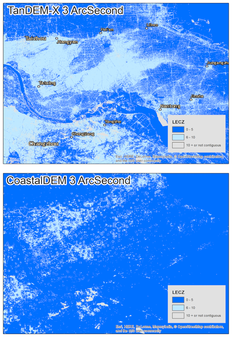
Figure B2 Raw TanDEM-X captures roadways, whereas CoastalDEM seems to capture agricultural land uses.

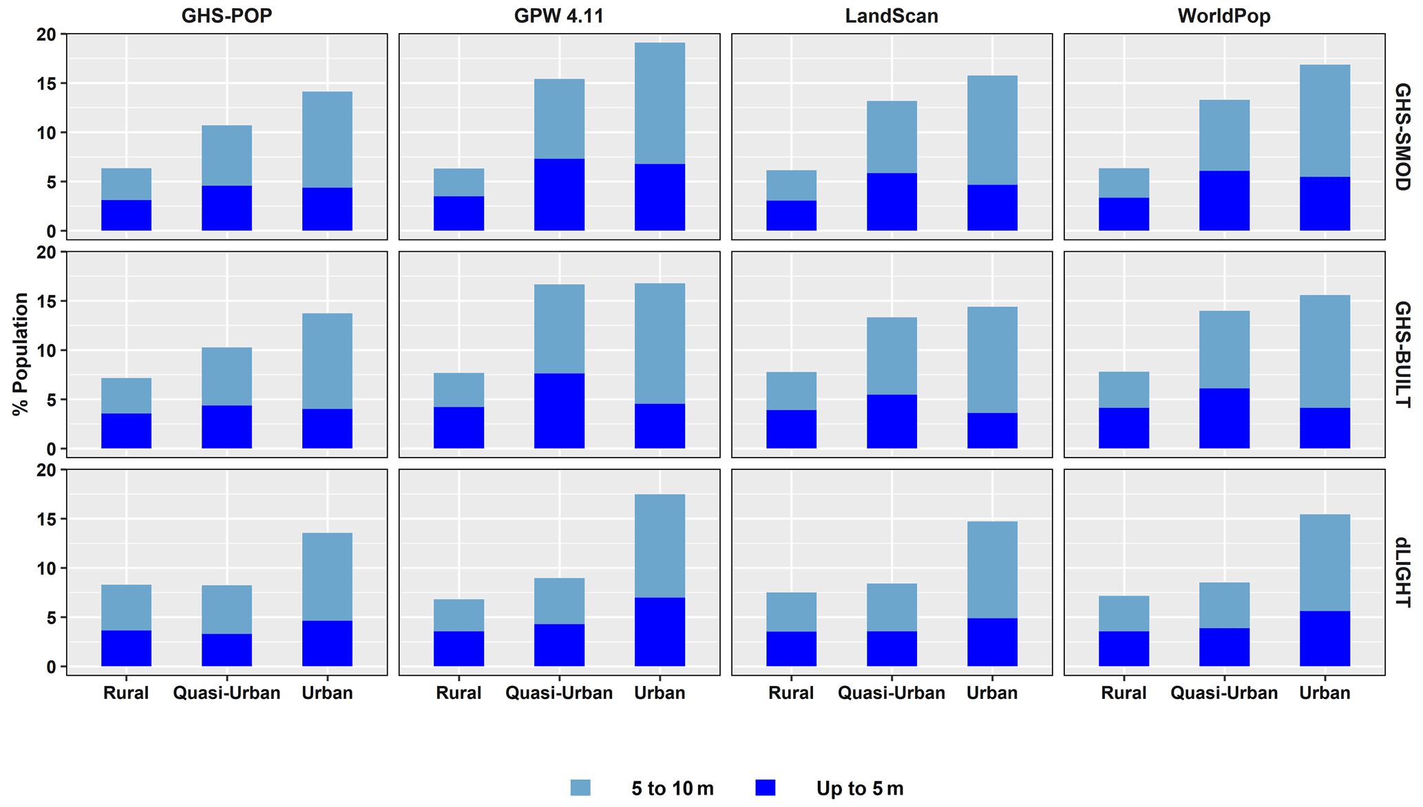
Figure B3 Proportion of the global population in each urban class (urban, quasi-urban and rural) in the ≤ 5 and 5–10 m LECZ, by each respective urban–rural class, according to different population and urban-proxy data sets, 2015. (MERIT DEM is used for LECZ delineation.)

Figure B4 Population density of urban, quasi-urban and rural by urban–rural classes, by LECZ using MERIT DEM.

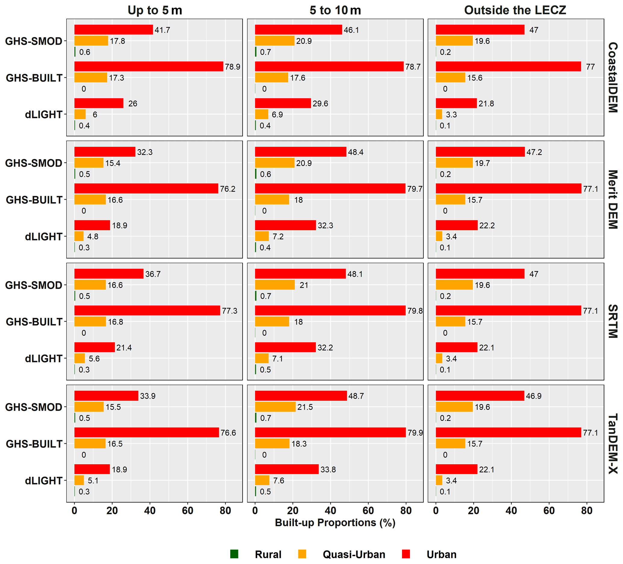
Figure B5 Built-up density (%) of urban, quasi-urban and rural by urban–rural classes, by urban-proxy and election data sets inside and outside of the LECZ.

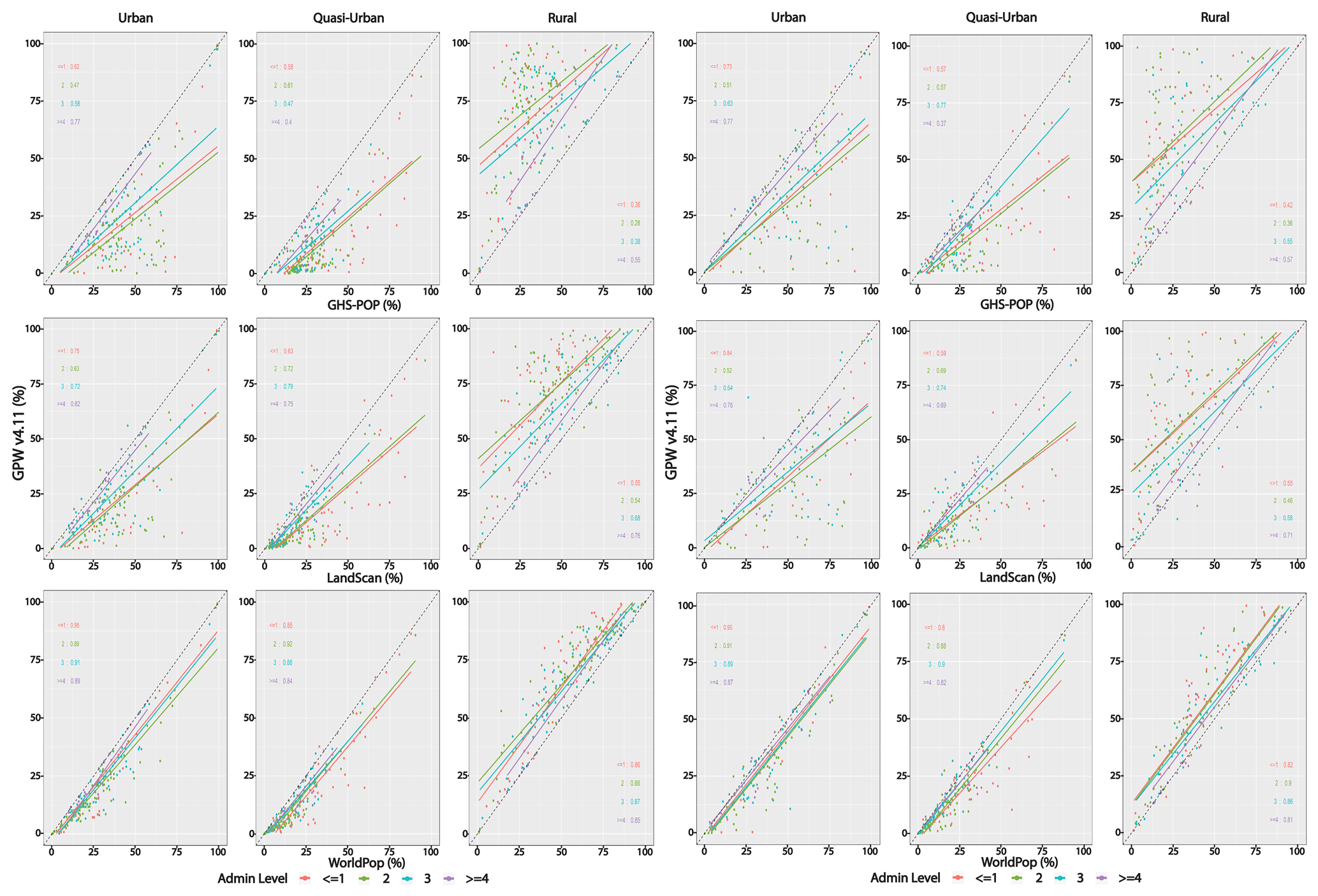
Figure B6 Comparison of population data sources by level of input unit in GPW, by urban–rural classes and urban-proxy data sets (GHS-SMOD). The left panel shows all land areas; the right panel shows area only in the ≤ 10 m LECZ.

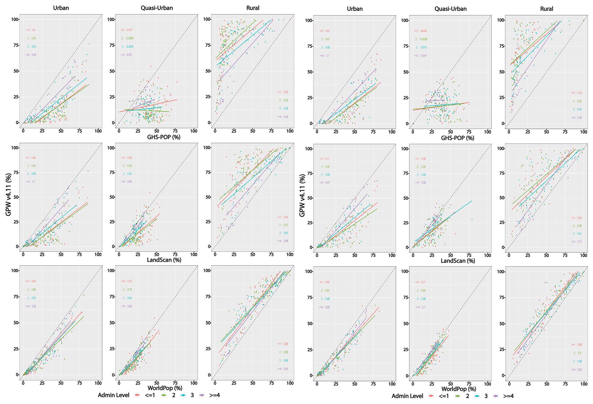
Figure B7 Comparison of population data sources by level of input unit in GPW, by urban–rural classes and urban-proxy data sets (GHS-BUILT). The left panel shows all land areas; the right panel shows only under 10 m (LECZ).

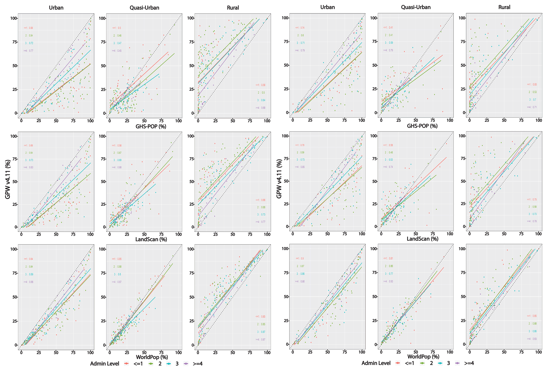
Figure B8 Comparison of population data sources by level of input unit in GPW, by urban–rural classes and urban-proxy data sets (dLIGHT). The left panel shows all land areas; the right panel shows only under 10 m (LECZ).

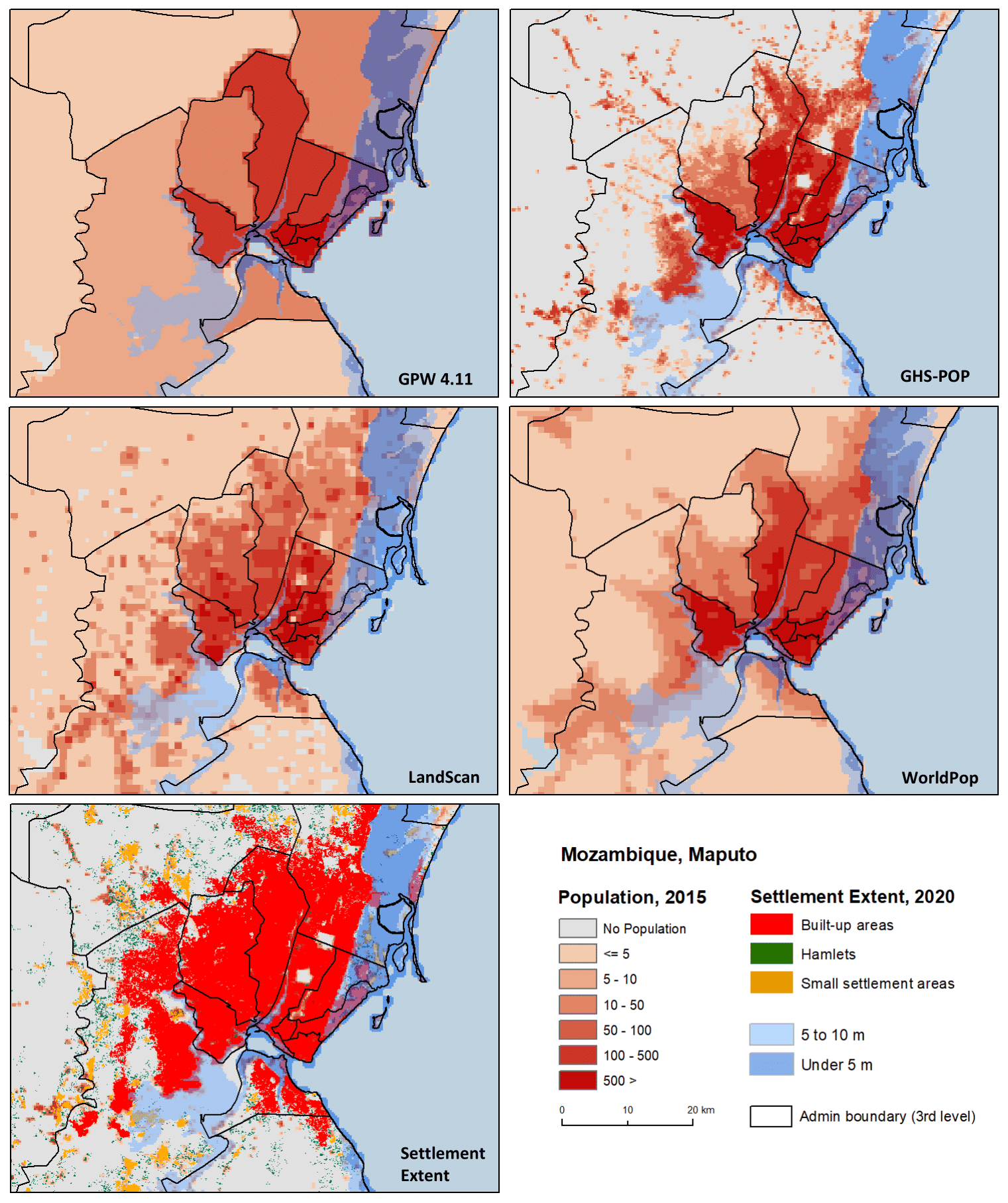
Figure B9 Comparison of population distributions by population data sources shown with administrative boundaries and GRID3 building-footprint-derived settlement extent data, Maputo and surrounding region.

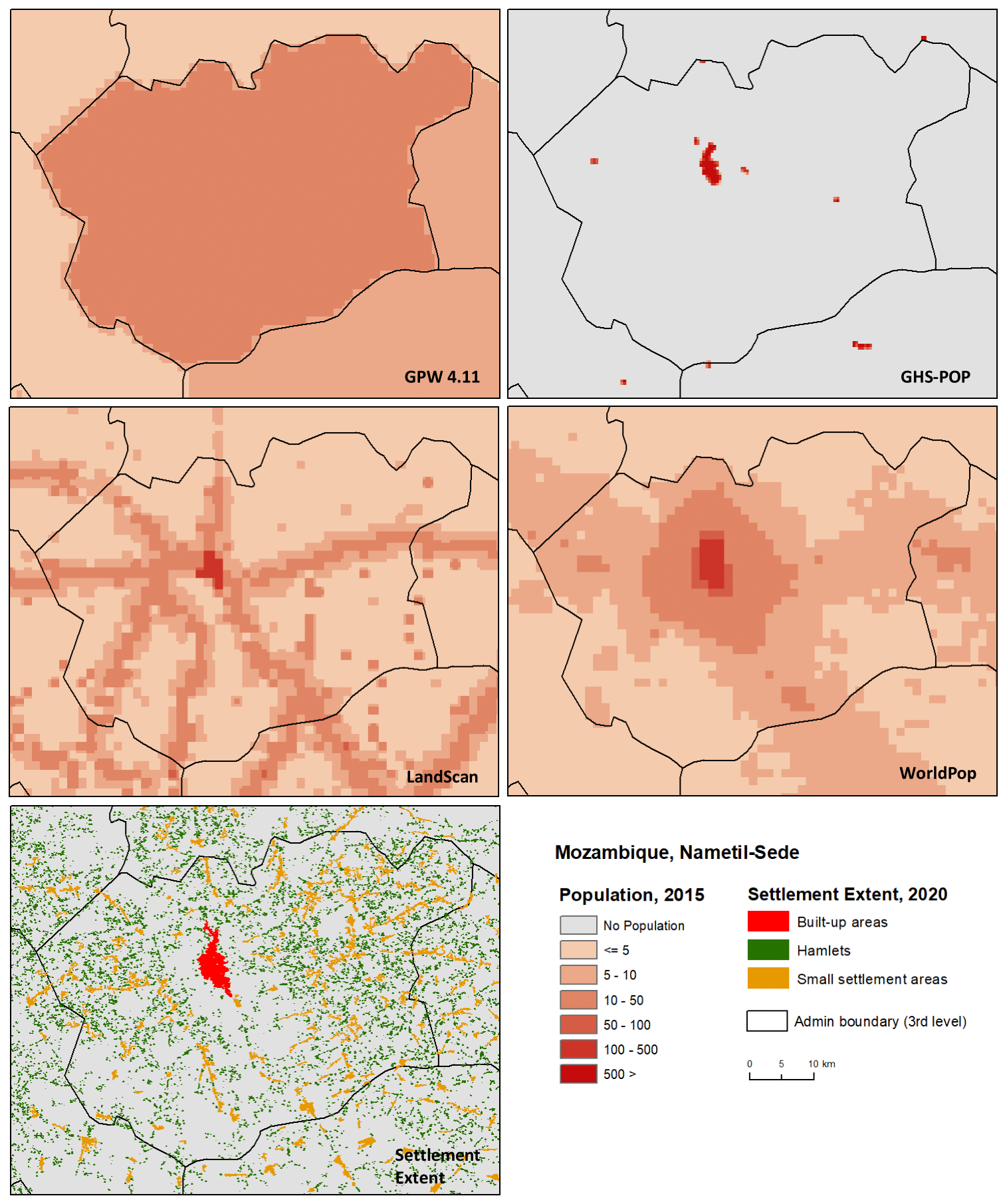
Figure B10 Comparison of population distributions by population data sources shown with administrative boundaries and GRID3 building-footprint-derived settlement extent data, Nametil-Sede and surrounding region.

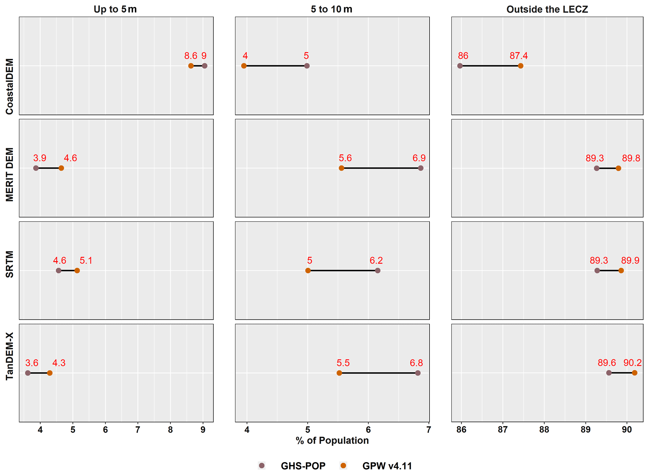
Figure B11 Estimates of population in different LECZs, by elevation and population data sources, 1990.

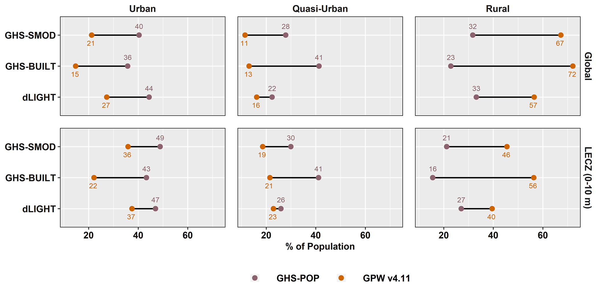
Figure B12 Percent of total population, by urban–rural classes, using different urban-proxy and population data sources, globally and in the ≤ 10 m LECZ (using MERIT DEM), 1990.

Appendix C

Table C1 Comparison of population data sources by level of input unit in GPW, by urban–rural classes and urban-proxy data sets, in the LECZ.

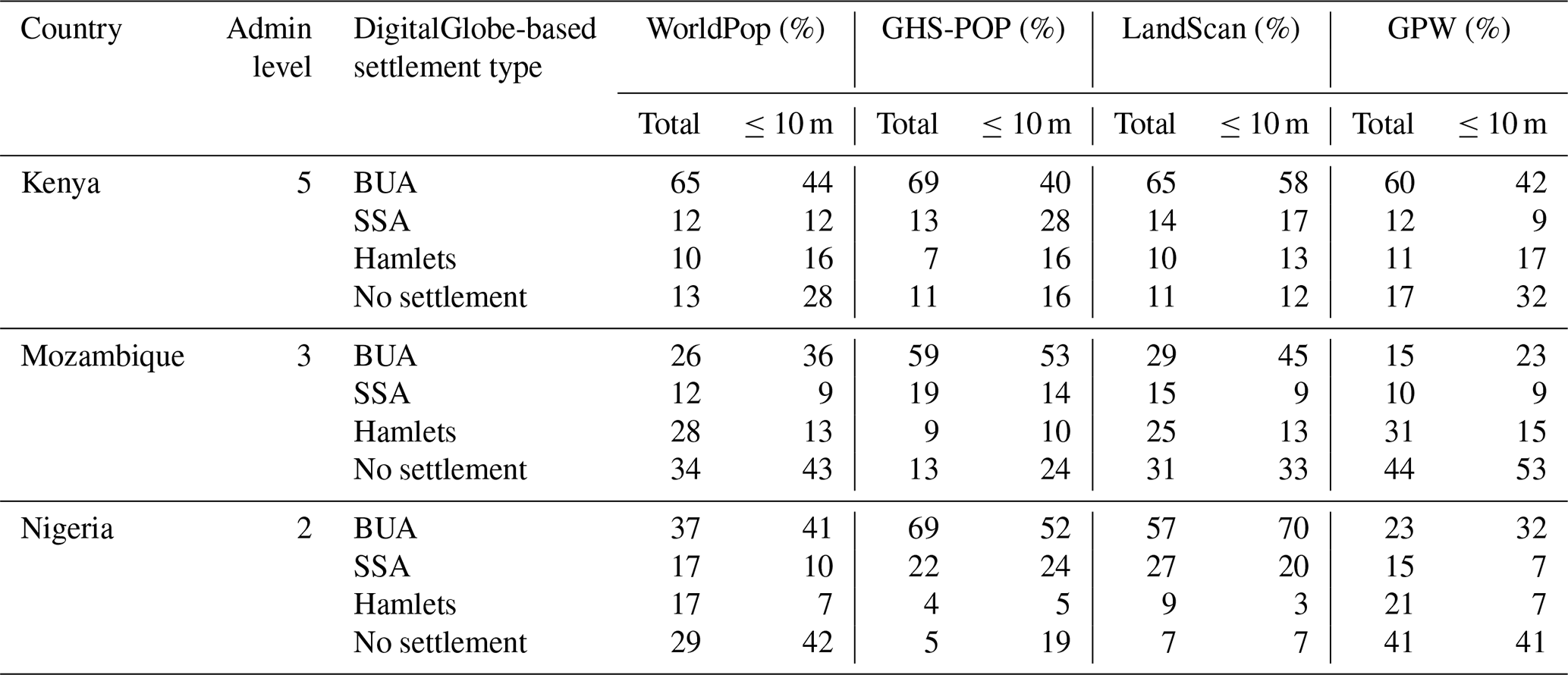
BUA (built-up area): building count above 3000. SSA (small settlement area): building count between 50 and 3000. Hamlet: building count less than 30. Admin level: level of administrative unit used in GPW (CIESIN and Novel-T, 2020). GRID3 Mozambique Settlement Extents Version 02, Alpha. Palisades, NY: Geo-Referenced Infrastructure and Demographic Data for Development.